An Introduction to Interacting Simulated Annealing

An Introduction to Interacting Simulated

Annealing

Juergen Gall, Bodo Rosenhahn, and Hans-Peter Seidel

Max-Planck Institute for Computer ScienceStuhlsatzenhausweg 85, 66123 Saarbrucken, Germany

Abstract. Human motion capturing can be regarded as an optimiza-tion problem where one searches for the pose that minimizes a previouslydefined error function based on some image features. Most approachesfor solving this problem use iterative methods like gradient descent ap-proaches. They work quite well as long as they do not get distracted by lo-cal optima. We introduce a novel approach for global optimization that issuitable for the tasks as they occur during human motion capturing. Wecall the method interacting simulated annealing since it is based on an in-teracting particle system that converges to the global optimum similar tosimulated annealing. We provide a detailed mathematical discussion thatincludes convergence results and annealing properties. Moreover, we givetwo examples that demonstrate possible applications of the algorithm,namely a global optimization problem and a multi-view human motioncapturing task including segmentation, prediction, and prior knowledge.A quantative error analysis also indicates the performance and the ro-bustness of the interacting simulated annealing algorithm.

1 Introduction

1.1 Motivation

Optimization problems arise in many applications of computer vision. In poseestimation, e.g. [28], and human motion capturing, e.g. [31], functions are mini-mized at various processing steps. For example, the marker-less motion capturesystem [26] minimizes in a first step an energy function for the segmentation. In asecond step, correspondences between the segmented image and a 3D model areestablished. The optimal pose is then estimated by minimizing the error givenby the correspondences. These optimization problems also occur, for instance,in model fitting [17, 31]. The problems are mostly solved by iterative methods asgradient descent approaches. The methods work very well as long as the start-ing point is near the global optimum, however, they get easily stuck in a localoptimum. In order to deal with it, several random selected starting points areused and the best solution is selected in the hope that at least one of them isnear enough to the global optimum, cf. [26]. Although it improves the results inmany cases, it does not ensure that the global optimum is found.In this chapter, we introduce a global optimization method based on an inter-acting particle system that overcomes the dilemma of local optima and that is

2 J. Gall, B. Rosenhahn and H.-P. Seidel

suitable for the optimization problems as they arise in human motion captur-ing. In contrast to many other optimization algorithms, a distribution insteadof a single value is approximated by a particle representation similar to particlefilters [10]. This property is beneficial, particularly, for tracking where the rightparameters are not always exact at the global optimum depending on the imagefeatures that are used.

1.2 Related Work

A popular global optimization method inspired by statistical mechanics is knownas simulated annealing [14, 18]. Similar to our approach, a function V ≥ 0 inter-preted as energy is minimized by means of an unnormalized Boltzmann-Gibbsmeasure that is defined in terms of V and an inverse temperature β > 0 by

g(dx) = exp (−β V (x)) λ(dx), (1.1)

where λ is the Lebesgue measure. This measure has the property that the prob-ability mass concentrates at the global minimum of V as β → ∞.The key idea behind simulated annealing is taking a random walk through thesearch space while β is successively increased. The probability of accepting anew value in the space is given by the Boltzmann-Gibbs distribution. Whilevalues with less energy than the current value are accepted with probabilityone, the probability that values with higher energy are accepted decreases asβ increases. Other related approaches are fast simulated annealing [30] using aCauchy-Lorentz distribution and generalized simulated annealing [32] based onTsallis statistics.Interacting particle systems [19] approximate a distribution of interest by a finitenumber of weighted random variables X (i) called particles. Provided that theweights Π(i) are normalized such that

∑Π(i) = 1, the set of weighted particles

determines a random probability measures by

n∑

i=1

Π(i)δX(i) . (1.2)

Depending on the weighting function and the distribution of the particles, themeasure converges to a distribution η as n tends to infinity. When the par-ticles are identically independently distributed according to η and uniformlyweighted, i.e. Π(i) = 1/n, the convergence follows directly from the law of largenumbers [3].Interacting particle systems are mostly known in computer vision as particlefilter [10] where they are applied for solving non-linear, non-Gaussian filteringproblems. However, these systems also apply for trapping analysis, evolutionaryalgorithms, statistics [19], and optimization as we demonstrate in this chapter.They usually consist of two steps as illustrated in Figure 1. During a selec-tion step, the particles are weighted according to a weighting function and thenresampled with respect to their weights, where particles with a great weightgenerate more offspring than particles with lower weight. In a second step, theparticles mutate or are diffused.

Interacting Simulated Annealing 3

Resampling:

particle

weighted particle

weighting functionWeighting:

Diffusion:

Fig. 1. Operation of an interacting particle system. After weighting the particles (blackcircles), the particles are resampled and diffused (gray circles).

1.3 Interaction and Annealing

Simulated annealing approaches are designed for global optimization, i.e. forsearching the global optimum in the entire search space. Since they are not ca-pable of focusing the search on some regions of interest in dependency on theprevious visited values, they are not suitable for tasks in human motion cap-turing. Our approach, in contrast, is based on an interacting particle systemthat uses Boltzmann-Gibbs measures (1.1) similar to simulated annealing. Thiscombination ensures not only the annealing property as we will show, but alsoexploits the distribution of the particles in the space as measure for the uncer-tainty in an estimate. The latter allows an automatic adaption of the search onregions of interest during the optimization process. The principle of the annealingeffect is illustrated in Figure 2.A first attempt to fuse interaction and annealing strategies for human motioncapturing has become known as annealed particle filter [9]. Even though theheuristic is not based on a mathematical background, it already indicates thepotential of such combination. Indeed, the annealed particle filter can be re-garded as a special case of interacting simulated annealing where the particlesare predicted for each frame by a stochastic process, see Section 3.1.

1.4 Outline

The interacting annealing algorithm is introduced in Section 3.1 and its asymp-totic behavior is discussed in Section 3.2. The given convergence results are basedon Feynman-Kac models [19] which are outlined in Section 2. Since a generaltreatment including proofs is out of the scope of this introduction, we refer theinterested reader to [11] or [19]. While our approach is evaluated for a standardglobal optimization problem in Section 4.1, Section 4.2 demonstrates the per-formance of interacting simulated annealing in a complete marker-less human


Fig. 2. Illustration of the annealing effect with three runs. Due to annealing, the parti-cles migrate towards the global maximum without getting stuck in the local maximum.

motion capture system that includes segmentation, pose prediction and priorknowledge.

1.5 Notations

We always regard E as a subspace of Rd, and let B(E) denote its Borel σ-algebra.B(E) denotes the set of bounded measurable functions, δx is the Dirac measureconcentrated in x ∈ E, ‖ · ‖2 is the Euclidean norm, and ‖ · ‖∞ is the well-knownsupremum norm. Let f ∈ B(E), µ be a measure on E, and let K be a Markovkernel on E1. We write

〈µ, f〉 =

∫

E

f(x) µ(dx), 〈µ, K〉(B) =

∫

E

K(x, B) µ(dx) for B ∈ B(E).

Furthermore, U [0, 1] denotes the uniform distribution on the interval [0, 1] and

osc(ϕ) := supx,y∈E

|ϕ(x) − ϕ(y)| . (1.3)

is an upper bound for the oscillations of f .

2 Feynman-Kac Model

Let (Xt)t∈N0 be an E-valued Markov process with family of transition kernels(Kt)t∈N0 and initial distribution η0. We denote by Pη0 the distribution of the

1 A Markov kernel is a function K : E × B(E) → [0,∞] such that K(·, B) isB(E)-measurable ∀B and K(x, ·) is a probability measure ∀x. An example of aMarkov kernel is given in Equation (1.11). For more details on probability theoryand Markov kernels, we refer to [3].


Markov process, i.e. for t ∈ N0,

Pη0 (d(x0, x1, . . . , xt)) = Kt−1(xt−1, dxt) . . .K0(x0, dx1) η0(dx0),

and by Eη0 [·] the expectation with respect to Pη0 . The sequence of distributions(ηt)t∈N0 on E defined for any ϕ ∈ B(E) and t ∈ N0 as

〈ηt, ϕ〉 :=〈γt, ϕ〉〈γt, 1〉

, 〈γt, ϕ〉 := Eη0

[ϕ (Xt) exp

(−

t−1∑

s=0

βs V (Xs)

)],

is called the Feynman-Kac model associated with the pair (exp(−βt V ), Kt).The Feynman-Kac model as defined above satisfies the recursion relation

ηt+1 = 〈Ψt(ηt), Kt〉, (1.4)

where the Boltzmann-Gibbs transformation Ψt is defined by

Ψt (ηt) (dyt) =Eη0

[exp

(−∑t−1

s=0 βs V (Xs))]

Eη0

[exp

(−∑t

s=0 βs V (Xs))] exp (−βt Vt(yt)) ηt(dyt).

The particle approximation of the flow (1.4) depends on a chosen family ofMarkov transition kernels (Kt,ηt

)t∈N0 satisfying the compatibility condition

〈Ψt (ηt) , Kt〉 := 〈ηt, Kt,ηt〉.

A family (Kt,ηt)t∈N0 of kernels is not uniquely determined by these conditions.

As in [19, Chapter 2.5.3], we choose

Kt,ηt= St,ηt

Kt, (1.5)

where

St,ηt(xt, dyt) = εt exp (−βt Vt(xt)) δxt

(dyt)

+ (1 − εt exp (−βt Vt(xt))) Ψt (ηt) (dyt), (1.6)

with εt ≥ 0 and εt ‖exp(−βt V )‖∞ ≤ 1. The parameters εt may depend on thecurrent distribution ηt.

3 Interacting Simulated Annealing

Similar to simulated annealing, one can define an annealing scheme 0 ≤ β0 ≤β1 ≤ . . . ≤ βt in order to search for the global minimum of an energy functionV . Under some conditions that will be stated in Section 3.2, the flow of theFeynman-Kac distribution becomes concentrated in the region of global minimaof V as t goes to infinity. Since it is not possible to sample from the distributiondirectly, the flow is approximated by a particle set as it is done by a particlefilter. We call the algorithm for the flow approximation interacting simulatedannealing (ISA).


3.1 Algorithm

The particle approximation for the Feynman-Kac model is completely describedby the Equation (1.5). The particle system is initialized by n identically, indepen-

dently distributed random variables X(i)0 with common law η0 determining the

random probability measure ηn0 :=

∑ni=1 δ

X(i)0

/n. Since Kt,ηtcan be regarded as

the composition of a pair of selection and mutation Markov kernels, we split thetransitions into the following two steps

ηnt

Selection−−−−−−−−→ ηnt

Mutation−−−−−−−−→ ηnt+1,

where

ηnt :=

1

n

n∑

i=1

δX

(i)t

, ηnt :=

1

n

n∑

i=1

δX

(i)t

.

During the selection step each particle X(i)t evolves according to the Markov

transition kernel St,ηnt(X

(i)t , ·). That means X

(i)t is accepted with probability

εt exp(−βt V (X(i)t )), and we set X

(i)t = X

(i)t . Otherwise, X

(i)t is randomly se-

lected with distribution

n∑

i=1

exp(−βt V (X(i)t ))

∑nj=1 exp(−βt V (X

(j)t ))

δX

(i)t

.

The mutation step consists in letting each selected particle X(i)t evolve according

to the Markov transition kernel Kt(X(i)t , ·).

Algorithm 1 Interacting Simulated Annealing Algorithm

Requires: parameters (εt)t∈N0 , number of particles n, initial distribution η0, energyfunction V , annealing scheme (βt)t∈N0 and transitions (Kt)t∈N0

1. Initialization– Sample x

(i)0 from η0 for all i

2. Selection– Set π(i) ← exp(−βt V (x

(i)t )) for all i

– For i from 1 to n:Sample κ from U [0, 1]If κ ≤ εtπ

(i) then? Set x

(i)t ← x

(i)t

Else? Set x

(i)t ← x

(j)t with probability π(j)

P

nk=1

π(k)

3. Mutation– Sample x

(i)t+1 from Kt(x

(i)t , ·) for all i and go to step 2


There are several ways to choose the parameter εt of the selection kernel (1.6)that defines the resampling procedure of the algorithm, cf. [19]. If

εt := 0 ∀t, (1.7)

the selection can be done by multinomial resampling. Provided that2

n ≥ supt

(exp(βt osc(V )) ,

another selection kernel is given by

εt(ηt) :=1

n 〈ηt, exp(−βt V )〉 . (1.8)

In this case the expression εtπ(i) in Algorithm 1 is replaced by π(i)/

∑nk=1 π(k).

A third kernel is determined by

εt(ηt) :=1

inf y ∈ R : ηt (x ∈ E : exp(−βt V (x)) > y) = 0 , (1.9)

yielding the expression π(i)/ max1≤k≤n π(k) instead of εtπ(i).

Pierre del Moral showed in [19, Chapter 9.4] that for any t ∈ N0 and ϕ ∈ B(E)the sequence of random variables

√n(〈ηn

t , ϕ〉 − 〈ηt, ϕ〉)

converges in law to a Gaussian random variable W when the selection kernel(1.6) is used to approximate the flow (1.4). Moreover, it turns out that when(1.8) is chosen, the variance of W is strictly smaller than in the case with εt = 0.We remark that the annealed particle filter [9] relies on interacting simulatedannealing with εt = 0. The operation of the method is illustrated by

ηnt

Prediction−−−−−−−−→ ηnt+1

ISA−−−−−−−−→ ηnt+1.

The ISA is initialized by the predicted particles X(i)t+1 and performs M times the

selection and mutation steps. Afterwards the particles X(i)t+1 are obtained by an

additional selection. This shows that the annealed particle filter uses a simulatedannealing principle to locate the global minimum of a function V at each timestep.

3.2 Convergence

This section discusses the asymptotic behavior of the interacting simulated an-nealing algorithm. For this purpose, we introduce some definitions in accordancewith [19] and [15].

2 The inequality satisfies the condition εt ‖exp(−βt V )‖∞≤ 1 for Equation (1.6).


Definition 1. A kernel K on E is called mixing if there exists a constant 0 <ε < 1 such that

K(x1, ·) ≥ ε K(x2, ·) ∀x1, x2 ∈ E. (1.10)

The condition can typically only be established when E ⊂ Rd is a bounded

subset, which is the case in many applications like human motion capturing. Forexample the (bounded) Gaussian distribution on E

K(x, B) :=1

Z

∫

B

exp

(−1

2(x − y)T Σ−1 (x − y)

)dy, (1.11)

where Z :=∫

E exp(− 12 (x − y)T Σ−1 (x − y) dy, is mixing if and only if E is

bounded. Moreover, a Gaussian with a high variance satisfies the mixing condi-tion with a larger ε than a Gaussian with lower variance.

Definition 2. The Dobrushin contraction coefficient of a kernel K on E is de-fined by

β(K) := supx1,x2∈E

supB∈B(E)

|K(x1, B) − K(x2, B)| . (1.12)

Furthermore, β(K) ∈ [0, 1] and β(K1K2) ≤ β(K1) β(K2).

When the kernel M is a composition of several mixing Markov kernels, i.e. M :=KsKs+1 . . . Kt, and each kernel Kk satisfies the mixing condition for some εk,the Dobrushin contraction coefficient can be estimated by β(M) ≤ ∏t

k=s(1−εk).The asymptotic behavior of the interacting simulated annealing algorithm isaffected by the convergence of the flow of the Feynman-Kac distribution (1.4) tothe region of global minima of V as t tends to infinity and by the convergence ofthe particle approximation to the Feynman-Kac distribution at each time step tas the number of particles n tends to infinity.

Convergence of the flow We suppose that Kt = K is a Markov kernel sat-isfying the mixing condition (1.10) for an ε ∈ (0, 1) and osc(V ) < ∞. A timemesh is defined by

t(n) := n(1 + bc(ε)c) c(ε) := (1 − ln(ε/2))/ε2 for n ∈ N0. (1.13)

Let 0 ≤ β0 ≤ β1 . . . be an annealing scheme such that βt = βt(n+1) is constant inthe interval (t(n), t(n+1)]. Furthermore, we denote by ηt the Feynman-Kac dis-tribution after the selection step, i.e. ηt = Ψt(ηt). According to [19, Proposition6.3.2], we have

Theorem 1. Let b ∈ (0, 1) and βt(n+1) = (n + 1)b. Then for each δ > 0

limn→∞

ηt(n) (V ≥ V? + δ) = 0,

where V? = supv ≥ 0; V ≥ v a.e..The rate of convergence is d/n(1−b) where d is increasing with respect to b andc(ε) but does not depend on n as given in [19, Theorem 6.3.1]. This theorem es-tablishes that the flow of the Feynman-Kac distribution ηt becomes concentratedin the region of global minima as t → +∞.


Convergence of the particle approximation Del Moral established thefollowing convergence theorem [19, Theorem 7.4.4].

Theorem 2. For any ϕ ∈ B(E),

Eη0

[∣∣〈ηnt+1, ϕ〉 − 〈ηt+1, ϕ〉

∣∣] ≤ 2 osc(ϕ)√n

(1 +

t∑

s=0

rsβ(Ms)

),

where

rs := exp

(osc(V )

t∑

r=s

βr

),

Ms := KsKs+1 . . . Kt,

for 0 ≤ s ≤ t.

Assuming that the kernels Ks satisfy the mixing condition with εs, we get arough estimate for the number of particles

n ≥ 4 osc(ϕ)2

δ2

(1 +

t∑

s=0

exp

(osc(V )

t∑

r=s

βr

)t∏

k=s

(1 − εk)

)2

(1.14)

needed to achieve a mean error less than a given δ > 0.

Fig. 3. Impact of the mixing condition satisfied for εs = ε. Left: Parameter c(ε) ofthe time mesh (1.13). Right: Rough estimate for the number of particles needed toachieve a mean error less than δ = 0.1.

Optimal transition kernel The mixing condition is not only essential forthe convergence result of the flow as stated in Theorem 1 but also influencesthe time mesh by the parameter ε. In view of Equation (1.13), kernels with εclose to 1 are preferable, e.g. Gaussian kernels on a bounded set with a very


high variance. The right hand side of (1.14) can also be minimized if Markovkernels Ks are chosen such that the mixing condition is satisfied for a εs closeto 1, as shown in Figure 3. However, we have to consider two facts. First, theinequality in Theorem 2 provides an upper bound of the accumulated error ofthe particle approximation up to time t + 1. It is clear that the accumulation ofthe error is reduced when the particles are highly diffused, but it also means thatthe information carried by the particles from the previous time steps is mostlylost by the mutation. Secondly, we cannot sample from the measure ηt directly,instead we approximate it by n particles. Now the following problem arises. Themass of the measure concentrates on a small region of E on one hand and, onthe other hand, the particles are spread over E if ε is large. As a result we geta degenerated system where the weights of most of the particles are zero andthus the global minima are estimated inaccurately, particularly for small n. Ifwe choose a kernel with small ε in contrast, the convergence rate of the flow isvery slow. Since neither of them is suitable in practice, we suggest a dynamicvariance scheme instead of a fixed kernel K.It can implemented by Gaussian kernels Kt with covariance matrices Σt propor-tional to the sample covariance after resampling. That is, for a constant c > 0,

Σt :=c

n − 1

n∑

i=1

(x(i)t − µt)ρ (x

(i)t − µt)

Tρ , µt :=

1

n

n∑

i=1

x(i)t , (1.15)

where ((x)ρ)k = max(xk, ρ) for a ρ > 0. The value ρ ensures that the variancedoes not become zero. The elements off the diagonal are usually set to zero, inorder to reduce computation time.

Optimal parameters The computation cost of the interacting simulated an-nealing algorithm with n particles and T annealing runs is O(nT ), where

nT := n · T . (1.16)

While more particles give a better particle approximation of the Feynman-Kacdistribution, the flow becomes more concentrated in the region of global minimaas the number of annealing runs increases. Therefore, finding the optimal valuesis a trade-off between the convergence of the flow and the convergence of theparticle approximation provided that nT is fixed.Another important parameter of the algorithm is the annealing scheme. Thescheme given in Theorem 1 ensures convergence for any energy function V —even for the worst one in the sense of optimization — as long as osc(V ) < ∞but is too slow for most applications, as it is the case for simulated annealing.In our experiments the schemes

βt = ln(t + b) for some b > 1 (logarithmic), (1.17)

βt = (t + 1)b for some b ∈ (0, 1) (polynomial) (1.18)

performed well. Note that in contrast to the time mesh (1.13) the schemes arenot anymore constant on a time interval.


Even though a complete evaluation of the various parameters is out of the scopeof this introduction, the examples given in the following section demonstratesettings that perform well, in particular for human motion capturing.

4 Examples

4.1 Global Optimization

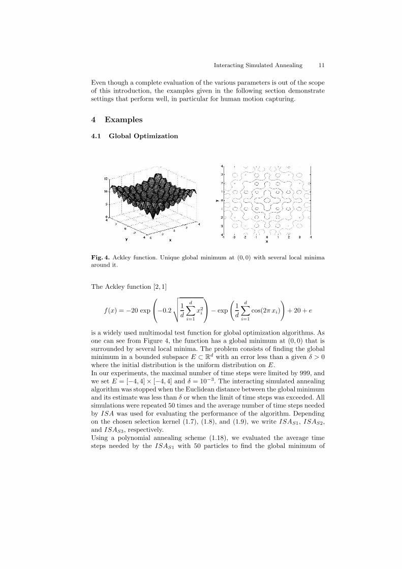
Fig. 4. Ackley function. Unique global minimum at (0, 0) with several local minimaaround it.

The Ackley function [2, 1]

f(x) = −20 exp

−0.2

√√√√1

d

d∑

i=1

x2i

− exp

(1

d

d∑

i=1

cos(2π xi)

)+ 20 + e

is a widely used multimodal test function for global optimization algorithms. Asone can see from Figure 4, the function has a global minimum at (0, 0) that issurrounded by several local minima. The problem consists of finding the globalminimum in a bounded subspace E ⊂ R

d with an error less than a given δ > 0where the initial distribution is the uniform distribution on E.In our experiments, the maximal number of time steps were limited by 999, andwe set E = [−4, 4] × [−4, 4] and δ = 10−3. The interacting simulated annealingalgorithm was stopped when the Euclidean distance between the global minimumand its estimate was less than δ or when the limit of time steps was exceeded. Allsimulations were repeated 50 times and the average number of time steps neededby ISA was used for evaluating the performance of the algorithm. Dependingon the chosen selection kernel (1.7), (1.8), and (1.9), we write ISAS1, ISAS2,and ISAS3, respectively.Using a polynomial annealing scheme (1.18), we evaluated the average timesteps needed by the ISAS1 with 50 particles to find the global minimum of


Fig. 5. Average time steps needed to find global minimum with error less than 10−3

with respect to the parameters b and c.

the Ackley function. The results with respect to the parameter of the annealingscheme, b ∈ [0.1, 0.999], and the parameter of the dynamic variance scheme,c ∈ [0.1, 3], are given in Figure 5. The algorithm performed best with a fastincreasing annealing scheme, i.e. b > 0.9, and with c in the range 0.5− 1.0. Theplots in Figure 5 also reveal that the annealing scheme has greater impact onthe performance than the factor c. When the annealing scheme increases slowly,i.e. b < 0.2, the global minimum was actually not located within the given limitfor all 50 simulations.

Ackley Ackley with noise

ISAS1 ISAS2 ISAS3 ISAS1 ISAS2 ISAS3

b 0.993 0.987 0.984 0.25 0.35 0.27

c 0.8 0.7 0.7 0.7 0.7 0.9

t 14.34 15.14 14.58 7.36 7.54 7.5

Table 1. Parameters b and c with lowest average time t for different selection kernels.

The best results with parameters b and c for ISAS1, ISAS2, and ISAS3 arelisted in Table 1. The optimal parameters for the three selection kernels arequite similar and the differences of the average time steps are marginal.

In a second experiment, we fixed the parameters b and c, where we used thevalues from Table 1, and varied the number of particles in the range 4 − 200with step size 2. The results for ISAS1 are shown in Figure 6. While the averageof time steps declines rapidly for n ≤ 20, it is hardly reduced for n ≥ 40. Hence,nt and thus the computation cost are lowest in the range 20 − 40. This showsthat a minimum number of particles are required to achieve a success rate of100%, i.e., the limit was not exceeded for all simulations. In this example, thesuccess rate was 100% for n ≥ 10. Furthermore, it indicates that the average of


Fig. 6. Left: Average time steps needed to find global minimum with respect to numberof particles. Right: Computation cost.

time steps is significantly higher for n less than the optimal number of particles.The results for ISAS1, ISAS2, and ISAS3 are quite similar. The best resultsare listed in Table 2.

Ackley Ackley with noise

ISAS1 ISAS2 ISAS3 ISAS1 ISAS2 ISAS3

n 30 30 28 50 50 26

t 22.4 20.3 21.54 7.36 7.54 12.54

nt 672 609 603.12 368 377 326.04

Table 2. Number of particles with lowest average computation cost for different selec-tion kernels.

The ability of dealing with noisy energy functions is one of the strength of ISAas we will demonstrate. This property is very usefull for applications where themeasurement of the energy of a particle is distorted by noise. On the left handside of Figure 7, the Ackley function is distorted by Gaussian noise with standarddeviation 0.5, i.e.,

fW (x) := max 0, f(x) + W , W ∼ N(0, 0.52).

As one can see, the noise deforms the shape of the function and changes theregion of global minima. In our experiments, the ISA was stopped when thetrue global minimum at (0, 0) was found with an accuracy of δ = 0.01.For evaluating the parameters b and c, we set n = 50. As shown on the righthand side of Figure 7, the best results were obtained by annealing schemeswith b ∈ [0.22, 0.26] and c ∈ [0.6, 0.9]. In contrast to the undistorted Ackleyfunction, annealing schemes that increase slowly performed better than the fastone. Indeed, the success rate dropped below 100% for b ≥ 0.5. The reason is


obvious from the left hand side of Figure 7. Due to the noise, the particles aremore easily distracted and a fast annealing scheme diminishes the possibilityof escaping from the local minima. The optimal parameters for the dynamicvariance scheme are hardly affected by the noise.

Fig. 7. Left: Ackley function distorted by Gaussian noise with standard deviation 0.5.Right: Average time steps needed to find global minimum with error less than 10−2

with respect to the parameters b and c.

The best parameters for ISAS1, ISAS2, and ISAS3 are listed in the Tables 1and 2. Except for ISAS3, the optimal number of particles is higher than it isthe case for the simulations without noise. The minimal number of particles toachieve a success rate of 100% also increased, e.g. 28 for ISAS1. We remark thatISAS3 required the least number of particles for a complete success rate, namely4 for the undistorted energy function and 22 in the noisy case.We finish this section by illustrating two examples of energy function wherethe dynamic variance schemes might not be suitable. On the left hand sideof Figure 8, an energy function with shape similar to the Ackley function isdrawn. The dynamic variance schemes perform well for this type of functionwith an unique global minimum with several local minima around it. Due to thescheme, the search focuses on the region near the global minimum after sometime steps. The second function, see Figure 8(b), has several, widely separatedglobal minima yielding a high variance of the particles even in the case that theparticles are near to the global minima. Moreover, when the region of globalminima is regarded as a sum of Dirac measures, the mean is not essentially aglobal minimum. In the last example shown on the right hand side of Figure 8,the global minimum is a small peak far away from a broad basin with a localminimum. When all particles fall into the basin, the dynamic variance schemesfocus the search on the region near the local minimum and it takes a long timeto discover the global minimum.In most optimization problems arising in the field of computer vision, however,the first case occurs where the dynamic variance schemes perform well. Oneapplication is human motion capturing which we will discuss in the next section.


(a) (b) (c)

Fig. 8. Different cases of energy functions. (a) Optimal for dynamic variance schemes.An unique global minimum with several local minima around it. (b) Several globalminima that are widely separated. This yields a high variance even in the case that theparticles are near to the global minima. (c) The global minimum is a small peak faraway from a broad basin. When all particles fall into the basin, the dynamic varianceschemes focus the search on the basin.

4.2 Human Motion Capture

Fig. 9. From left to right: (a) Original image. (b) Silhouette. (c) Estimated pose.(d) 3D model.

In our second experiment, we apply the interacting simulated annealing algo-rithm to model-based 3D tracking of the lower part of a human body, see Fig-ure 9(a). This means that the 3D rigid body motion (RBM) and the joint angles,also called the pose, are estimated by exploiting the known 3D model of thetracked object. The mesh model illustrated in Figure 9(d) has 18 degrees of free-dom (DoF), namely 6 for the rigid body motion and 12 for the joint angles of thehip, knees, and feet. Although a marker-less motion capture system is discussed,markers are also sticked to the target object in order to provide a quantitativecomparison with a commercial marker based system.

Using the extracted silhouette as shown in Figure 9(b), one can define an energyfunction V which describes the difference between the silhouette and an esti-mated pose. The pose that fits the silhouette best takes the global minimum ofthe energy function, which is searched by the ISA. The estimated pose projectedonto the image plane is displayed in Figure 9(c).


Pose representation There are several ways to represent the pose of an object,e.g. Euler angles, quaternions [16], twists [20], or the axis-angle representation.The ISA requires from the representation that primarily the mean but also thevariance can be at least well approximated. For this purpose, we have chosenthe axis-angle representation of the absolute rigid body motion M given by the6D vector (θω, t) with

ω = (ω1, ω2, ω3), ‖ω‖2 = 1 and t = (t1, t2, t3).

Using the exponential, M is expressed by

M =

(exp (θω) t

0 1

), ω =

0 −ω3 ω2

ω3 0 −ω1

−ω2 ω1 0

. (1.19)

While t is the absolute position in the world coordinate system, the rotationvector θω describes a rotation by an angle θ ∈ R about the rotation axis ω. Thefunction exp (θω) can be efficiently computed by the Rodriguez formula [20].Given a rigid body motion defined by a rotation matrix R ∈ SO(3) and atranslation vector t ∈ R

3, the rotation vector is constructed according to [20] asfollows: When R is the identity matrix, θ is set to 0. For the other case, θ andthe rotation axis ω are given by

θ = cos−1

(trace(R) − 1

2

), ω =

1

2 sin(θ)

r32 − r23

r13 − r31

r21 − r12

. (1.20)

We write log(R) for the inverse mapping of the exponential.

The mean of a set of rotations ri in the axis-angle representation can be com-puted by using the exponential and the logarithm as described in [22, 23]. Theidea is to find a geodesic on the Riemannian manifold determined by the set of3D rotations. When the geodesic starting from the mean rotation in the manifoldis mapped by the logarithm onto the tangent space at the mean, it is a straightline starting at the origin. The tangent space is called exponential chart .

Hence, using the notations

r2 ? r1 = log (exp(r2) · exp(r1)) , r−11 = log

(exp(r1)

T)

for the rotation vectors r1 and r2, the mean rotation r satisfies

∑

i

(r−1 ? ri

)= 0. (1.21)

Weighting each rotation with πi, yields the least squares problem:

1

2

∑

i

πi

∥∥r−1 ? ri

∥∥2

2→ min. (1.22)


The weighted mean can thus be estimated by

rt+1 = rt ?

(∑i πi

(r−1t ? ri

)∑

i πi

). (1.23)

The gradient descent method takes about 5 iterations until it converges.The variance and the normal density on a Riemannian manifold can also beapproximated, cf. [24]. Since, however, the variance is only used for diffusing theparticles, a very accurate approximation is not needed. Hence, the variance of aset of rotations ri is calculated in the Euclidean space R

3.The twist representation used in [7, 26] and in Chapters RosenhahnetAl,BroxetAl

is quite similar. Instead of a separation between the translation t and the rota-tion r, it describes a screw motion where the motion velocity θ also affects thetranslation. A twist ξ ∈ se(3)3 is represented by

θξ = θ

(ω v0 0

), (1.24)

where exp(θξ) is a rigid body motion.The logarithm of a rigid body motion M ∈ SE(3) is the following transformation:

θω = log(R), v = A−1t, (1.25)

where

A = (I − exp(θω))ω + ωωT θ (1.26)

is obtained from the Rodriguez formula. This follows from the fact, that the twomatrices which comprise A have mutually orthogonal null spaces when θ 6= 0.Hence, Av = 0 ⇔ v = 0.We remark that the two representations are identical for the joints where only arotation around a known axis is performed. Furthermore, a linearization is notneeded for the ISA in contrast to the pose estimation as described in Chap-ters RosenhahnetAl and BroxetAl.

Pose prediction The ISA can be combined with a pose prediction in two ways.When the dynamics are modelled by a Markov process for example, the particlesof the current frame can be stored and predicted for the next frame accordingto the process as done in [12]. In this case, the ISA is already initialized bythe predicted particles. But when the prediction is time consuming or when thehistory of previous poses is needed, only the estimate is predicted. The ISAis then initialized by diffusing the particles around the predicted estimate. Thereinitialization of the particles is necessary for example when the prediction isbased on local descriptors [13] or optical flow as discussed in Chapter BroxetAl

and [5].

3 se(3) is the Lie algebra that corresponds to the Lie group SE(3).


In our example, the pose is predicted by an autoregression that takes the globalrigid body motions Pi of the last N frames into account [13]. For this purpose,we use a set of twists ξi = log(PiP

−1i−1) representing the relative motions. By

expressing the local rigid body motion as a screw action, the spatial velocity canbe represented by the twist of the screw, see [20] for details.

M

P P

P3

M

ξ

ξ’

O1

ξ1

22

1

1 2 ξ2’

M3

Fig. 10. Transformation of rigid body motions from prior data Pi in a current worldcoordinate system M1. A proper scaling of the twists results in a proper damping.

In order to generate a suited rigid body motion from the motion history, a screwmotion needs to be represented with respect to another coordinate system. Letξ ∈ se(3) be a twist given in a coordinate frame A. Then for any G ∈ SE(3),

which transforms a coordinate frame A to B, is GξG−1 a twist with the twistcoordinates given in the coordinate frame B, see [20] for details. The mapping

ξ 7−→ GξG−1 is called the adjoint transformation associated with G.Let ξ1 = log(P2P

−11 ) be the twist representing the relative motion from P1 to P2.

This transformation can be expressed as local transformation in the current co-ordinate system M1 by the adjoint transformation associated with G = M1P

−11 .

The new twist is then given by ξ′1 = Gξ1G−1. The advantage of the twist rep-

resentation is now, that the twists can be scaled by a factor 0 ≤ λi ≤ 1 todamp the local rigid body motion, i.e. ξ′i = GλiξiG

−1. For given λi such that∑i λi = 1, the predicted pose is obtained by the rigid body transformation

exp(ξ′N ) exp(ξ′N−1) . . . exp(ξ′1). (1.27)

Energy function The energy function V of a particle x, which is used forour example, depends on the extracted silhouette and on some learned priorknowledge as in [12], but it is defined in a different way.Silhouette: First of all, the silhouette is extracted from an image by a level setbased segmentation as in [8, 27]. We state the energy functional E for conve-nience only and refer the reader to Chapter BroxetAl where the segmentationis described in detail. Let Ωi be the image domain of view i and let Φi

0(x ) bethe contour of the predicted pose in Ωi. In order to obtain the silhouettes for all


r views, the energy functional E(x, Φ1, . . . , Φr) =∑r

i=1 E(x, Φi) is minimzed,where

E(x, Φi) = −∫

H(Φi) ln pi1 + (1 − H(Φi)) ln pi

2 dx

+ ν

∫

Ωi

∣∣∇H(Φi)∣∣ dx + λ

∫

Ωi

(Φi − Φi

0(x ))2

dx. (1.28)

In our experiments, we weighted the smoothness term with ν = 4 and the shapeprior with λ = 0.04.After the segmentation, 3D-2D correspondences between the 3D model (Xi) anda 2D image (xi) are established by the projected vertices of the 3D mesh thatare part of the model contour and their closest points of the extracted contourthat are determined by a combination of an iterated closest point algorithm [4]and an optic flow based shape registration [25]. More details about the shapematching are given in Chapter RosenhahnetAl. We write each correspondenceas pair (Xi, xi) of homogeneous coordinates.Each image point xi defines a projection ray that can be represented as Pluckerline [20] determined by a unique vector ni and a moment mi such that x× ni −mi = 0 for all x on the 3D line. Furthermore,

‖x × ni − mi‖2 (1.29)

is the norm of the perpendicular error vector between the line and a point x ∈ R3.

As we already mentioned, a joint j is represented by the rotation angle θj .Hence, we write M(ω, t) for the rigid body motion and M(θj) for the joints.Furthermore, we have to consider the kinematic chain of articulated objects. LetXi be a point on the limb ki whose position is influenced by si joints in a certainorder. The inverse order of these joints is then given by the mapping ιki

, e.g.,a point on the left shank is influenced by the left knee joint ιki

(4) and by thethree joints of the left hip ιki

(3), ιki(2), and ιki

(1).Hence, the pose estimation consists of finding a pose x such that the error

errS(x, i) :=

∥∥∥∥(M(ω, t)M(θιki

(1)) . . . M(θιki(si))Xi

)3×1

× ni − mi

∥∥∥∥2

(1.30)

is minimal for all pairs, where (·)3×1 denotes the transformation from homoge-neous coordinates back to non-homogeneous coordinates.Prior Knowledge: Using prior knowledge about the probability of a certainpose can stabilize the pose estimation as shown in [12] and [6]. The prior ensuresthat particles representing a familiar pose are favored in problematic situations,e.g., when the observed object is partially occluded. As discussed in ChapterBroxetAl, the probability of the various poses is learned from N training sam-ples, where the density is estimated by a Parzen-Rosenblatt estimator [21, 29]with a Gaussian kernel

ppose(x) =1

(2 π σ2)d/2 N

N∑

i=1

exp

(−‖xi − x‖2

2

2 σ2

). (1.31)


In our experiments, we chose the window size σ as the maximum second nearestneighbor distance between all training samples as in [12].Incorporating the learned probability of the poses in the energy function hasadditional advantages. First, it already incorporates correlations between theparameters of a pose – and thus of a particle – yielding an energy function thatis closer to the model and the observed object. Moreover, it can be regarded as asoft constraint that includes anatomical constraints, e.g. by the limited freedomof joints movement, and that prevents the estimates from self-intersections sinceunrealistic and impossible poses cannot be contained in the training data.Altogether, the energy function V of a particle x is defined by

V (x) :=1

l

l∑

i=1

errS(x, i)2 − η ln(ppose(x)), (1.32)

where l is the number of correspondences. In our experiments, we set η = 8.

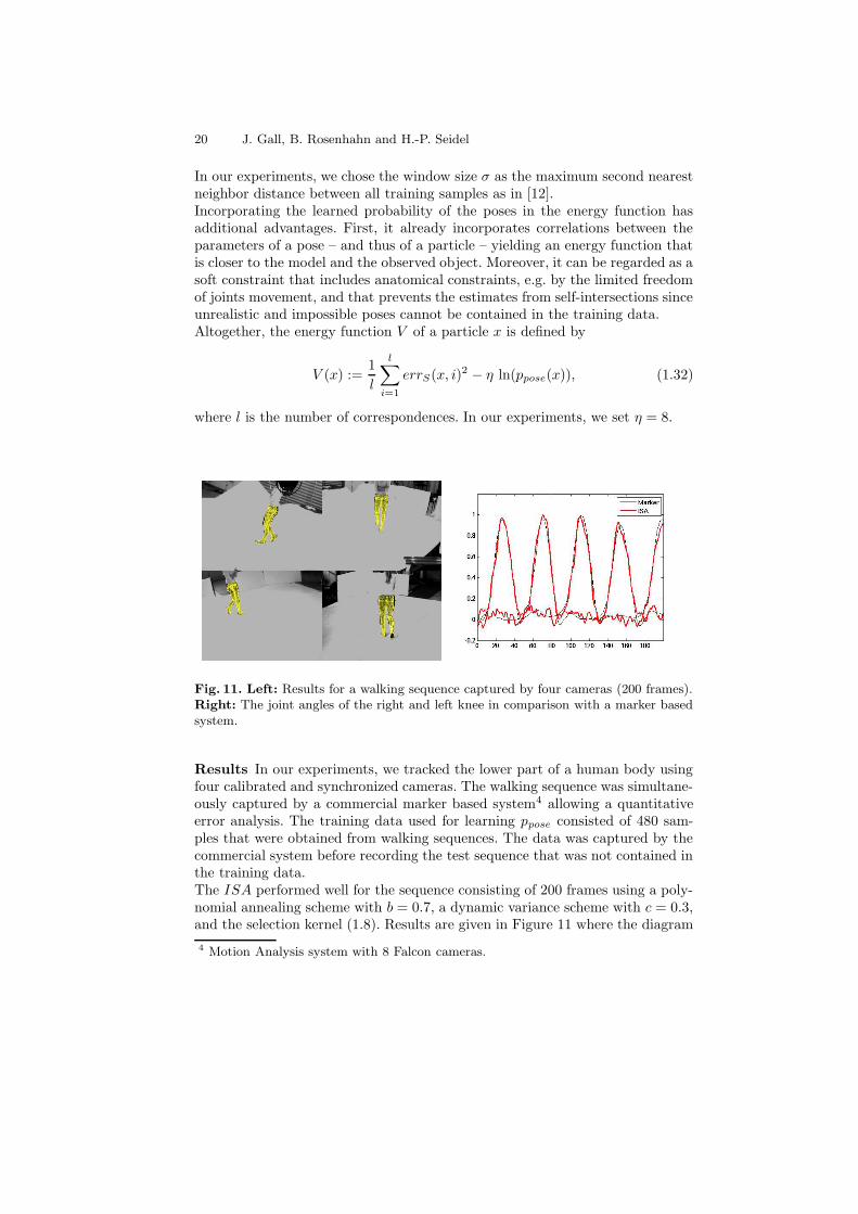
Fig. 11. Left: Results for a walking sequence captured by four cameras (200 frames).Right: The joint angles of the right and left knee in comparison with a marker basedsystem.

Results In our experiments, we tracked the lower part of a human body usingfour calibrated and synchronized cameras. The walking sequence was simultane-ously captured by a commercial marker based system4 allowing a quantitativeerror analysis. The training data used for learning ppose consisted of 480 sam-ples that were obtained from walking sequences. The data was captured by thecommercial system before recording the test sequence that was not contained inthe training data.The ISA performed well for the sequence consisting of 200 frames using a poly-nomial annealing scheme with b = 0.7, a dynamic variance scheme with c = 0.3,and the selection kernel (1.8). Results are given in Figure 11 where the diagram

4 Motion Analysis system with 8 Falcon cameras.


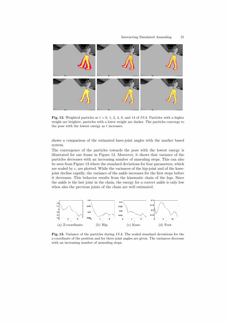
Fig. 12. Weighted particles at t = 0, 1, 2, 4, 8, and 14 of ISA. Particles with a higherweight are brighter, particles with a lower weight are darker. The particles converge tothe pose with the lowest energy as t increases.

shows a comparison of the estimated knee-joint angles with the marker basedsystem.

The convergence of the particles towards the pose with the lowest energy isillustrated for one frame in Figure 12. Moreover, it shows that variance of theparticles decreases with an increasing number of annealing steps. This can alsobe seen from Figure 13 where the standard deviations for four parameters, whichare scaled by c, are plotted. While the variances of the hip-joint and of the knee-joint decline rapidly, the variance of the ankle increases for the first steps beforeit decreases. This behavior results from the kinematic chain of the legs. Sincethe ankle is the last joint in the chain, the energy for a correct ankle is only lowwhen also the previous joints of the chain are well estimated.

(a) Z-coordinate. (b) Hip. (c) Knee. (d) Foot.

Fig. 13. Variance of the particles during ISA. The scaled standard deviations for thez-coordinate of the position and for three joint angles are given. The variances decreasewith an increasing number of annealing steps.


Fig. 14. Left: Energy of estimate for walking sequence (200 frames). Right: Error ofestimate (left and right knee).

On the right hand side of Figure 14, the energy of the estimate during trackingis plotted. We also plotted the root-mean-square error of the estimated knee-angles for comparison where we used the results from the marker based system asground truth with an accuracy of 3 degrees. For n = 250 and T = 15, we achievedan overall root-mean-square error of 2.74 degrees. The error was still below 3degrees with 375 particles and T = 7, i.e. nT = 2625. With this setting, the ISAtook 7−8 seconds for approximately 3900 correspondences that were establishedin the 4 images of one frame. The whole system including segmentation, took 61seconds for one frame. For comparison, the iterative method as used in ChapterRosenhahnetAl took 59 seconds with an error of 2.4 degrees. However, wehave to remark that for this sequence the iterative method performed very well.This becomes clear from the fact that no additional random starting pointswere needed. Nevertheless, it demonstrates that the ISA can keep up even insituations that are perfect for iterative methods.

Fig. 15. Left: Random pixel noise. Right: Occlusions by random rectangles.


Figures 16 and 17 show the robustness in the presence of noise and occlusions.For the first sequence, each frame was independently distorted by 70% pixelnoise, i.e., each pixel value was replaced with probability 0.7 by a value uni-formly sampled from the interval [0, 255]. The second sequence was distorted byoccluding rectangles of random size, position, and gray value, where the edgelengths were in the range from 1 to 40. The knee angles are plotted in Figure 15.The root mean-square errors were 2.97 degrees, 4.51 degrees, and 5.21 degreesfor 50% noise, 70% noise, and 35 occluding rectangles, respectively.

Fig. 16. Estimates for a sequence distorted by 70% random pixel noise. One view offrames 35, 65, 95, 125, 155, and 185 is shown.

5 Discussion

We introduced a novel approach for global optimization, termed interacting sim-ulated annealing (ISA), that converges to the global optimum. It is based onan interacting particle system where the particles are weighted according toBoltzmann-Gibbs measures determined by an energy function and an increasingannealing scheme.The variance of the particles provides a good measure of the confidence in theestimate. If the particles are all near the global optimum, the variance is lowand only a low diffusion of the particles is required. The estimate, in contrast, isunreliable for particles with an high variance. This knowledge is integrated viadynamic variance schemes that focus the search on regions of interest dependingon the confidence in the current estimate. The performance and the potential ofISA was demonstrated by means of two applications.The first example showed that our approach can deal with local optima andsolves the optimization problem well even for noisy measurements. However, we


Fig. 17. Estimates for a sequence with occlusions by 35 rectangles with random size,color, and position. One view of frames 35, 65, 95, 125, 155, and 185 is shown.

also provided some limitations of the dynamic variance schemes where standardglobal optimization methods might perform better. Since a comparison withother global optimization algorithm is out of the scope of this introduction, thiswill be done in future.

The application to multi-view human motion capturing, demonstrated the em-bedding of ISA into a complex system. The tracking system included silhouetteextraction by a level-set method, a pose prediction by an auto-regression, andprior knowledge learned from training data. Providing an error analysis, wedemonstrated the accuracy and the robustness of the system in the presence ofnoise and occlusions. Even though we considered only a relative simple walkingsequence for demonstration, it already indicates the potential of ISA for humanmotion capturing. Indeed, a comparison with an iterative approach revealed thaton the one hand global optimization methods cannot perform better than localoptimization methods when local optima are not problematic as it is the casefor the walking sequence, but on the other hand it also showed that the ISA cankeep up with the iterative method. We expect therefore that the ISA performsbetter for faster movements, more complex motion patterns, and human modelswith higher degrees of freedom. In addition, the introduced implementation ofthe tracking system with ISA has one essential drawback for the performance.While the pose estimation is performed by a global optimization method, thesegmentation is still susceptible to local minima since the energy function (1.28)is minimized by a local optimization approach.

As part of future work, we will integrate ISA into the segmentation processto overcome the local optima problem in the whole system. Furthermore, anevaluation and a comparison with an iterative method needs to be done withsequences of different kinds of human motions and also when the segmentation


is independent of the pose estimation, e.g., as it is the case for backgroundsubtraction. Another improvement might be achieved by considering correlationsbetween the parameters of the particles for the dynamic variance schemes, wherean optimal trade-off between additional computation cost and increased accuracyneeds to be found.

Acknowledgments

Our research is funded by the Max-Planck Center for Visual Computing andCommunication. We thank Uwe Kersting for providing the walking sequence.

References

1. D. Ackley. A connectionist machine for genetic hillclimbing. Kluwer, Boston, 1987.2. T. Back and H.-P. Schwefel. An overview of evolutionary algorithms for parameter

optimization. Evolutionary Computation, 1:1–24, 1993.3. H. Bauer. Probability Theory. de Gruyter, Baton Rouge, 1996.4. P. Besl and N. McKay. A Method for Registration of 3-D Shapes. IEEE Transac-

tions on Pattern Analysis and Machine Intelligence, 14(2):239-256, 1992.5. T. Brox, B. Rosenhahn, D. Cremers, and H.-P. Seidel. High accuracy optical

flow serves 3-D pose tracking: exploiting contour and flow based constraints. InA. Leonardis, H. Bischof, and A. Pinz, editors, European Conference on ComputerVision (ECCV), LNCS 3952, pages 98–111. Springer, 2006.

6. T. Brox, B. Rosenhahn, U. Kersting, and D. Cremers. Nonparametric DensityEstimation for Human Pose Tracking. In Pattern Recognition (DAGM). LNCS4174, pages 546–555. Springer, 2006.

7. C. Bregler, J. Malik, and K. Pullen. Twist Based Acquisition and Tracking of An-imal and Human Kinematics. International Journal of Computer Vision, 56:179–194, 2004.

8. T. Brox, B. Rosenhahn, and J. Weickert. Three-dimensional shape knowledge forjoint image segmentation and pose estimation. In W. Kropatsch, R. Sablatnig,A. Hanbury, editors, Pattern Recognition (DAGM), LNCS 3663, pages 109–116.Springer, 2005.

9. J. Deutscher and I. Reid. Articulated body motion capture by stochastic search.International Journal of Computer Vision, 61(2):185–205, 2005.

10. A. Doucet, N. de Freitas, and N. Gordon, editors. Sequential Monte Carlo Methodsin Practice. Statistics for Engineering and Information Science. Springer, NewYork, 2001.

11. J. Gall, J. Potthoff, C. Schnoerr, B. Rosenhahn, and H.-P. Seidel. Interacting andAnnealing Particle Systems – Mathematics and Recipes. Journal of MathematicalImaging and Vision, 2007, To appear.

12. J. Gall, B. Rosenhahn, and T. Brox and H.-P. Seidel. Learning for Multi-View 3DTracking in the Context of Particle Filters. In International Symposium on VisualComputing (ISVC), LNCS 4292, pages 59–69. Springer, 2006.

13. J. Gall, B. Rosenhahn, and H.-P. Seidel. Robust Pose Estimation with 3D Tex-tured Models. In IEEE Pacific-Rim Symposium on Image and Video Technology(PSIVT), LNCS 4319, pages 84–95. Springer, 2006.


14. S. Geman and D. Geman. Stochastic relaxation, Gibbs distributions, and theBayesian restoration of images. IEEE Transactions on Pattern Analysis and Ma-chine Intelligence, 6(6):721–741, 1984.

15. B. Gidas. Topics in Contemporary Probability and Its Applications, Chapter 7:Metropolis-type Monte Carlo Simulation Algorithms and Simulated Annealing,pages 159–232. Probability and Stochastics Series. CRC Press, Boca Raton, 1995.

16. H. Goldstein. Classical Mechanics. Addison-Wesley, Reading, MA, second edition,1980.

17. D. Grest, D. Herzog, and R. Koch. Human Model Fitting from Monocular PostureImages. In G. Greiner, J. Hornegger, H. Niemann, and M. Stamminger, editors,Vision, Modeling, and Visualization. Akademische Verlagsgesellschaft Aka, 2005.

18. S. Kirkpatrick, C. Gelatt Jr., and M. Vecchi. Optimization by Simulated Annealing.Science, 220(4598):671–680, 1983.

19. P. Del Moral. Feynman-Kac Formulae. Genealogical and Interacting Particle Sys-tems with Applications. Probability and its Applications. Springer, New York,2004.

20. R.M. Murray, Z. Li, and S.S. Sastry. Mathematical Introduction to Robotic Manip-ulation. CRC Press, Baton Rouge, 1994.

21. E. Parzen. On estimation of a probability density function and mode. Annals ofMathematical Statistics, 33:1065–1076, 1962.

22. X. Pennec and N. Ayache. Uniform distribution, distance and expectation problemsfor geometric features processing. Journal of Mathematical Imaging and Vision,9(1):49–67, 1998.

23. X. Pennec. Computing the mean of geometric features: Application to the meanrotation. Rapport de Recherche RR–3371, INRIA, Sophia Antipolis, France, March1998.

24. X. Pennec. Intrinsic Statistics on Riemannian Manifolds: Basic Tools for GeometricMeasurements. Journal of Mathematical Imaging and Vision, 25(1):127–154, 2006.

25. B. Rosenhahn, T. Brox, D. Cremers, and H.-P. Seidel. A Comparison of ShapeMatching Methods for Contour Based Pose Estimation. In R. Reulke, U. Eckhardt,B. Flach, U. Knauer, and K. Polthier, editors, 11th International Workshop onCombinatorial Image Analysis (IWCIA), LNCS 4040, pages 263–276. Springer,2006.

26. B. Rosenhahn, T. Brox, U. Kersting, A. Smith, J. Gurney, and R. Klette. A systemfor marker-less human motion estimation. Kunstliche Intelligenz, 1:45–51, 2006.

27. B. Rosenhahn, T. Brox, and J. Weickert. Three-dimensional shape knowledge forjoint image segmentation and pose tracking. In International Journal of ComputerVision, 2006, To appear.

28. B. Rosenhahn, C. Perwass, and G. Sommer. Pose Estimation of Free-form Con-tours. International Journal of Computer Vision, 62(3):267–289, 2005.

29. F. Rosenblatt. Remarks on some nonparametric estimates of a density function.Annals of Mathematical Statistics, 27(3):832–837, 1956.

30. H. Szu and R. Hartley. Fast simulated annealing. Physic Letter A, 122:157–162,1987.

31. C. Theobalt, M. Magnor, P. Schueler, and H.P. Seidel. Combining 2D FeatureTracking and Volume Reconstruction for Online Video-Based Human Motion Cap-ture. In 10th Pacific Conference on Computer Graphics and Applications, pages96–103. IEEE Computer Society, 2002.

32. C. Tsallis and D.A. Stariolo. Generalized simulated annealing. Physica A, 233:395–406, 1996.

An Introduction to Interacting Simulated Annealing

Documents

Transcript of An Introduction to Interacting Simulated Annealing