An Introduction to Financial Mathematics

Sandeep JunejaTata Institute of Fundamental Research, Mumbai

juneja@tifr.res.in

1 Introduction

A wealthy acquaintance when recently asked about his profession reluctantly answered thathe is a middleman in drug trade and has made a fortune helping drugs reach Europeanmarkets from Latin America. When pressed further, he confessed that he was actuallya ‘quant’ in a huge wall street bank and used mathematics to price complex derivativesecurities. He lied simply to appear respectable! There you have it. Its not fashionableto be a financial mathematician these days. On the plus side, these quants or financialmathematicians on the wall street are sufficiently rich that they can literally afford to ignorefashions.

On a serious note, it is important to acknowledge that financial markets serve a funda-mental role in economic growth of nations by helping efficient allocation of investment ofindividuals to the most productive sectors of the economy. They also provide an avenuefor corporates to raise capital for productive ventures. Financial sector has seen enormousgrowth over the past thirty years in the developed world. This growth has been led by theinnovations in products referred to as financial derivatives that require great deal of mathe-matical sophistication and ingenuity in pricing and in creating an insurance or hedge againstassociated risks. This chapter briefly discusses some such popular derivatives including thosethat played a substantial role in the economic crisis of 2008. Our primary focus are the keyunderlying mathematical ideas that are used to price such derivatives. We present these ina somewhat simple setting.

Brief history: During the industrial revolution in Europe there existed great demand forsetting up huge industrial units. To raise capital, entrepreneurs came together to form jointpartnerships where they owned ‘shares’ of the newly formed company. Soon there were manysuch companies each with many shares held by public at large. This was facilitated by settingup of stock exchanges where these shares or stocks could be bought or sold. London stockexchange was first such institution, set up in 1773. Basic financial derivatives such as futureshave been around for some time (we do not discuss futures in this chapter; they are verysimilar to the forward contracts discussed below). The oldest and the largest futures andoptions exchange, The Chicago Board of Trade (CBOT), was established in 1848. Although,as we discuss later, activity in financial derivatives took off in a major way beginning theearly 1970’s.

1

Brief introduction to derivatives (see, e.g., [16] for a comprehensive overview): A deriva-tive is a financial instrument that derives its value from an ‘underlying’ more basic asset.For instance, consider a forward contract, a popular derivative, between two parties: Oneparty agrees to purchase from the other a specified asset at a particular time in future for aspecified price. For instance, Infosys, expecting income in dollars in future (with its expensesin rupees) may enter into a forward contract with ICICI bank that requires it to purchase aspecified amount of rupees, say Rs. 430 crores, using specified amount of dollars, say, $ 10crore, six months from now. Here, the fluctuations in more basic underlying exchange rategives value to the forward contract.

Options are popular derivatives that give buyer of this instrument an option but not anobligation to engage in specific transactions related to the underlying assets. For instance, acall option allows the buyer of this instrument an option but not an obligation to purchasean underlying asset at a specified strike price at a particular time in future, referred to astime to maturity. Seller of the option on the other hand is obligated to sell the underlyingasset to the buyer at the specified price if the buyer exercises the option. Seller of coursereceives the option price upfront for selling this derivative. For instance, one may purchasea call option on the Reliance stock, whose current value is, say, Rs. 1055, that gives theowner the option to purchase certain number of Reliance stocks, each at price Rs. 1100,three months from now. This option is valuable to the buyer at its time of maturity if thestock then is worth more than Rs. 1100. Otherwise this option is not worth exercising andhas value zero. In the earlier example, Infosys may instead prefer to purchase a call optionthat allows it the option to pay $10 crore to receive Rs. 430 crore six months from now.Infosys would then exercise this option if each dollar gets less than Rs. 43 in the market atthe option’s time to maturity.

Similarly, a put option gives the buyer of the instrument the option but not an obligationto sell an asset at a specified price at the time to maturity. These options are referred to asEuropean options if they can be exercised only at the time to maturity. American optionsallow an early exercise feature, that is, they can be exercised at any time up to the time tomaturity. There exist variants such as Bermudan options that can be exercised at a finitenumber of specified dates. Other popular options such as interest rate swaps, credit debtswaps (CDS’s) and collateralized debt obligations (CDOs) are discussed later in the chapter.Many more exotic options are not discussed in this chapter (see, e.g, Hull [16], Shreve [30]).

1.1 The no-arbitrage principle

Coming up with a fair price for such derivatives securities vexed the financial community rightup till early seventies when Black Scholes [3] came up with their famous formula for pricingEuropean options. Since then, the the literature on pricing financial derivatives has seena huge explosion and has played a major role in expansion of financial derivatives market.To put things in perspective, from a tiny market in the seventies, the market of financialderivatives has grown in notional amount to about $600 trillion in 2007. This compared tothe world GDP of order $45 trillion. Amongst financial derivatives, as of 2007, interest ratebased derivatives constitute about 72% of the market, currencies about 12%, and equitiesand commodities the remaining 16% (See, e.g., Baaquie [1]). Wall street employs thousandsof PhDs that use quantitative methods or ‘rocket science’ in derivatives pricing and related

2

=

Rs. Rs.

Figure 1: No Arbitrage Principle: Price of two liter ketchup bottle equals twice the price ofa one liter ketchup bottle, else ARBITRAGE, that is, profits can be made without any risk.

activities.‘No-arbitrage pricing principle’ is the key idea used by Black and Scholes to arrive at their

formula. It continues to be foundational for financial mathematics. Simply told, and as il-lustrated in Figure 1, this means that price of a two liter ketchup bottle should be twice theprice of a one liter ketchup bottle, otherwise by following the sacred mantra of buy low andsell high one can create an arbitrage, that is, instantaneously produce profits while takingzero risk. The no arbitrage principle precludes such free lunches and provides a surprisinglysophisticated methodology to price complex derivatives securities. This methodology relieson replicating pay-off from a derivative in every possible scenario by continuously and ap-propriately trading in the underlying more basic securities (transaction costs are assumedto be zero). Then, since the derivative and this trading strategy have identical payoffs, bythe no-arbitrage principle, they must have the same price. Hence, the cost of creating thistrading strategy provides the price of the derivative security.

In spite of the fact that continuous trading is an idealization and there always are smalltransaction costs, this pricing methodology approximates the practice well. Traders often sellcomplex risky derivatives and then dynamically trade in underlying securities in a mannerthat more or less cancels the risk arising from the derivative while incurring little trans-actional cost. Thus, from their viewpoint the price of the derivative must be at least theamount they need to cancel the associated risk. Competition ensures that they do not chargemuch higher than this price.

In practice one also expects no-arbitrage principle to hold as large banks typically havestrong groups of arbitragers that identify and quickly take advantage of such arbitrage op-portunities (again, by buying low and selling high) so that due to demand and supply theprices adjust and these opportunities become unavailable to common investors.

3

Fixed payment leg: Example, 6% of notional amount

Over many years

Floating payment leg: Example , six month LIBOR + 0.5%

Figure 2: Example illustrating interest rate swap cash-flows.

1.2 Popular derivatives

Interest rate swaps and swaptions, options on these swaps, are by far the most popularderivatives in the financial markets. The market size of these instruments was about $310trillion in 2007. Figure 2 shows an example of cash flows involved in an interest rate swap.Typically, for a specified duration of the swap (e.g., five years) one party pays a fixed rate(fraction) of a pre-specified notional amount at regular intervals (say, every quarter or halfyearly) to the other party, while the other party pays variable floating rate at the samefrequency to the first party. This variable rate may be a function of prevailing rates suchas the LIBOR rates (London Interbank Offered Rates; inter-bank borrowing rate amongstbanks in London). This is used by many companies to match their revenue streams to liabilitystreams. For instance, a pension fund may have fixed liabilities. However, the income theyearn may be a function of prevailing interest rates. By entering into a swap that pays at afixed rate they can reduce the variability of cash-flows and hence improve financial planning.

Swaptions give its buyer an option to enter into a swap at a particular date at a specifiedinterest rate structure. Due to their importance in the financial world, intricate mathematicalmodels have been developed to accurately price such interest rate instruments. Refer to, e.g.,[4], [5] for further details.

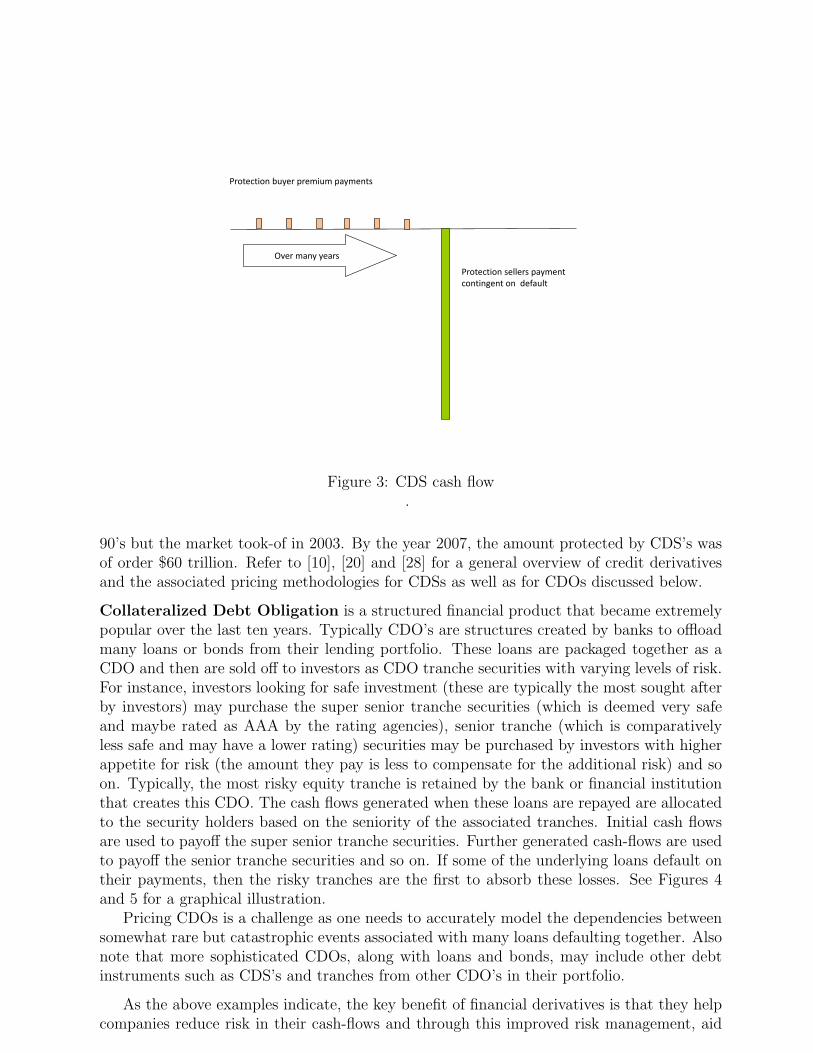
Credit Default Swap is a financial instrument whereby one party (A) buys protection (orinsurance) from another party (B) to protect against default by a third party (C). Defaultoccurs when a debtor C cannot meet its legal debt obligations. A pays a premium paymentat regular intervals (say, quarterly) to B up to the duration of the swap or until C defaults.During the swap duration, if C defaults, B pays A a certain amount and the swap terminates.These cash flows are depicted in Figure 3. Typically, A may hold a bond of C that has certainnominal value. If C defaults, then B provides protection against this default by purchasingthis much devalued bond from A at its higher nominal price. CDS’s were initiated in early

4

Protection buyer premium payments

Protection sellers payment contingent on default

Over many years

Figure 3: CDS cash flow.

90’s but the market took-of in 2003. By the year 2007, the amount protected by CDS’s wasof order $60 trillion. Refer to [10], [20] and [28] for a general overview of credit derivativesand the associated pricing methodologies for CDSs as well as for CDOs discussed below.

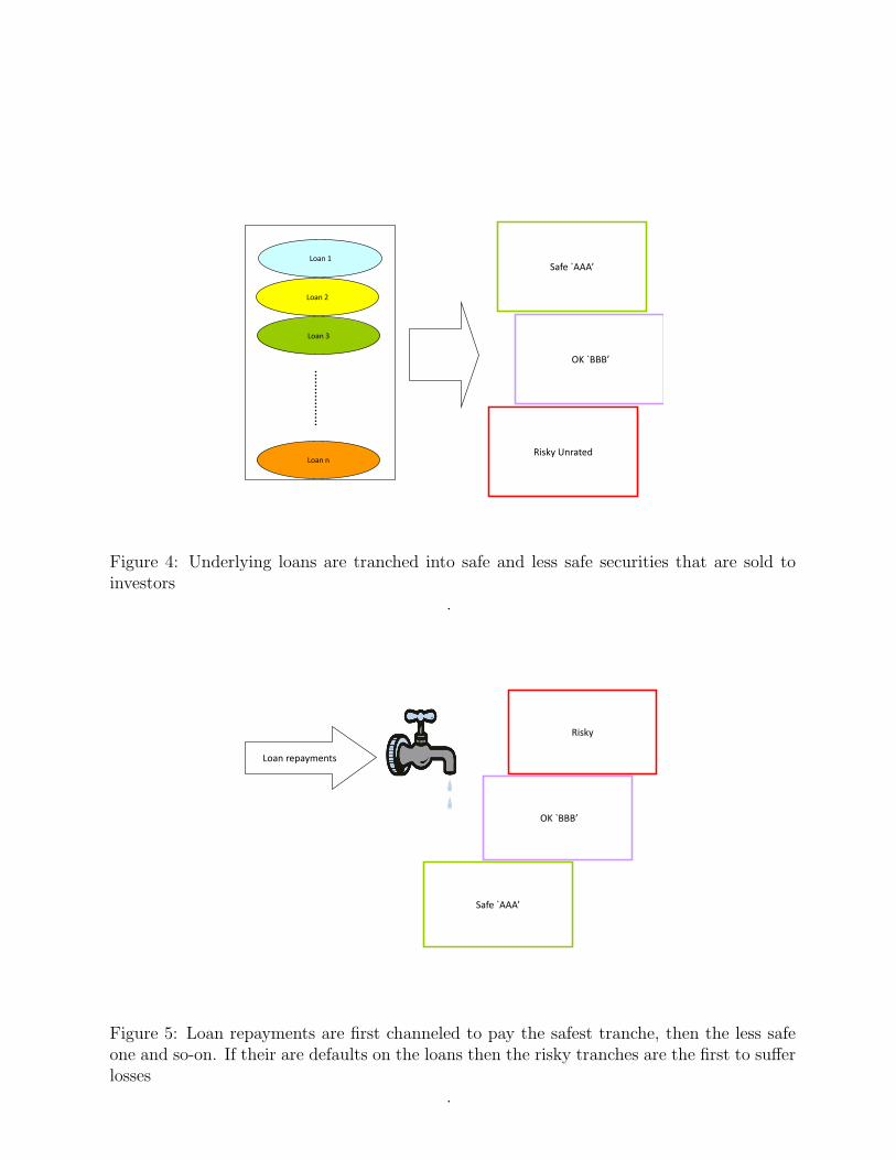
Collateralized Debt Obligation is a structured financial product that became extremelypopular over the last ten years. Typically CDO’s are structures created by banks to offloadmany loans or bonds from their lending portfolio. These loans are packaged together as aCDO and then are sold off to investors as CDO tranche securities with varying levels of risk.For instance, investors looking for safe investment (these are typically the most sought afterby investors) may purchase the super senior tranche securities (which is deemed very safeand maybe rated as AAA by the rating agencies), senior tranche (which is comparativelyless safe and may have a lower rating) securities may be purchased by investors with higherappetite for risk (the amount they pay is less to compensate for the additional risk) and soon. Typically, the most risky equity tranche is retained by the bank or financial institutionthat creates this CDO. The cash flows generated when these loans are repayed are allocatedto the security holders based on the seniority of the associated tranches. Initial cash flowsare used to payoff the super senior tranche securities. Further generated cash-flows are usedto payoff the senior tranche securities and so on. If some of the underlying loans default ontheir payments, then the risky tranches are the first to absorb these losses. See Figures 4and 5 for a graphical illustration.

Pricing CDOs is a challenge as one needs to accurately model the dependencies betweensomewhat rare but catastrophic events associated with many loans defaulting together. Alsonote that more sophisticated CDOs, along with loans and bonds, may include other debtinstruments such as CDS’s and tranches from other CDO’s in their portfolio.

As the above examples indicate, the key benefit of financial derivatives is that they helpcompanies reduce risk in their cash-flows and through this improved risk management, aid

5

Loan 1

Loan 2

Loan 3

Loan n

Safe `AAA’

OK `BBB’

Risky Unrated

Figure 4: Underlying loans are tranched into safe and less safe securities that are sold toinvestors

.

Safe `AAA’

OK `BBB’

Risky

Loan repayments

Figure 5: Loan repayments are first channeled to pay the safest tranche, then the less safeone and so-on. If their are defaults on the loans then the risky tranches are the first to sufferlosses

.

6

in financial planning, reduce the capital requirements and therefore enhance profitability.Currently, 92% of the top Fortune 500 companies engage in derivatives to better managetheir risk.

However, derivatives also make speculation easy. For instance, if one believes that aparticular stock price will rise, it is much cheaper and logistically efficient to place a big betby purchasing call options on that stock, then through acquiring the same number of stock,although the upside in both the cases is the same. This flexibility, as well as the underlyingcomplexity of some of the exotic derivatives such as CDOs, makes derivatives risky for theoverall economy. Warren Buffet famously referred to financial derivatives as time bombs andfinancial weapons of mass destruction. CDOs involving housing loans played a significantrole in the economic crisis of 2008. (See, e.g. Duffie [9]). The key reason being that whileit was difficult to precisely measure the risk in a CDO (due extremal dependence amongstloan defaults), CDOs gave a false sense of confidence to the loan originators that since therisk was being diversified away to investors, it was being mitigated. This in turn promptedacquisition of far riskier sub-prime loans that had very little chance of repayment.

In the remaining paper we focus on developing underlying ideas for pricing relatively sim-ple European options such as call or put options. In Section 2, we illustrate the no-arbitrageprinciple for a two-security-two-scenario-two-time-period Binomial tree toy model. In Sec-tion 3, we develop the pricing methodology for pricing European options in more realisticcontinuous-time-continuous-state framework. From a probabilistic viewpoint, this requiresconcepts of Brownian motion, stochastic Ito integrals, stochastic differential equations, Ito’sformula, martingale representation theorem and the Girsanov theorem. These concepts arebriefly introduced and used to develop the pricing theory. They remain fundamental to themodern finance pricing theory. We end with a brief conclusion in Section 4.

Financial mathematics is a vast area involving interesting mathematics in areas such asrisk management (see, e.g., Frey et. al. [22]) , calibration and estimation methodologiesfor financial models, econometric models for algorithmic trading as well as for forecastingand prediction (see, e.g., [6]), investment portfolio optimization (see, e.g., Meucci [23]) andoptimal stopping problem that arises in pricing American options (see, e.g., Glasserman[15]). In this chapter, however, we restrict our focus to some of the fundamental derivativepricing ideas.

2 Binomial Tree Model

We now illustrate how the no-arbitrage principle helps price options in a simple Binomial-treeor the ‘two-security-two scenario-two-time-period’ setting. This approach to price optionswas first proposed by Cox, Ross and Rubinstein [7] (see [29] for an excellent comprehensiveexposition of Binomial tree models).

Consider a simplified world consisting of two securities: The risky security or the stockand the risk free security or an investment in the safe money market. We observe these attime zero and at time ∆t. Suppose that stock has value S at time zero. At time ∆t twoscenarios up and down can occur (see Figure 6 for a graphical illustration): Scenario upoccurs with probability p ∈ (0, 1) and scenario down with probability 1− p. The stock takesvalue S exp(u∆t) in scenario up and S exp(d∆t) otherwise, where u > d. Money market

7

S 1

exp(rDt)

Cd

Cu

Risky security Risk free security

p

1-p exp(rDt)

Option Price ??

Option payoff in two scenarios

exp(uDt)

exp(dDt)

Figure 6: World comprising a risky security, a risk-free security and an option that needsto be priced. This world evolves in future for one time period where the risky securityand the option can take two possible values. No arbitrage principle that provides a uniqueprice for the option that is independent of p ∈ (0, 1), where (p, 1− p) denote the respectiveprobabilities of the two scenarios.

account has value 1 at time zero that increases to exp(r∆t) in both the scenarios at time∆t. Assume that any amount of both these assets can be borrowed or sold without anytransaction costs.

First note that the no-arbitrage principle implies that d < r < u. Otherwise, if r ≤ d,borrowing amount S from the money market and purchasing a stock with it, the investorearns at least S exp(d∆t) at time ∆t where his liability is S exp(r∆t). Thus with zeroinvestment he is guaranteed sure profit (at least with positive probability if r = d), violatingthe no-arbitrage condition. Similarly, if r ≥ u, then by short selling the stock (borrowingfrom an owner of this stock and selling it with a promise to return the stock to the originalowner at a later date) the investor gets amount S at time zero which he invests in the moneymarket. At time ∆t he gets S exp(r∆t) from this investment while his liability is at mostS exp(u∆t) (the price at which he can buy back the stock to close the short position), thusleading to an arbitrage.

Now consider an option that pays Cu in the up scenario and Cd in the down scenario. Forinstance, consider a call option that allows its owner an option to purchase the underlyingstock at the strike price K for some K ∈ (S exp(d∆t), S exp(u∆t)). In that case, Cu = S−Kdenotes the benefit to option owner in this scenario, and Cd = 0 underscores the fact thatoption owner would not like to purchase a risky security at value K, when he can purchase itfrom the market at a lower price S exp(d∆t). Hence, in this scenario the option is worthlessto its owner.

8

2.1 Pricing using no-arbitrage principle

The key question is to determine the fair price for such an option. A related problem isto ascertain how to cancel or hedge the risk that the seller of the option is exposed to bytaking appropriate positions in the underlying securities. Naively, one may consider theexpectation pCu + (1 − p)Cd suitably discounted (to account for time value of money andthe risk involved) to be the correct value of the option. As we shall see, this approach maylead to an incorrect price. In fact, in this simple world, the answer based on the no-arbitrageprinciple is straightforward and is independent of the probability p. To see this, we constructa portfolio of the stock and the risk free security that exactly replicates the payoff of theoption in the two scenarios. Then the value of this portfolio gives the correct option price.

Suppose we purchase α ∈ < number of stock and invest amount β ∈ < in the moneymarket, where α and β are chosen so that the resulting payoff matches the payoff from theoption at time ∆t in the two scenarios. That is,

αS exp(u∆t) + β exp(r∆t) = Cu

andαS exp(d∆t) + β exp(r∆t) = Cd.

Thus,

α =Cu − Cd

S(exp(u∆t)− exp(d∆t)),

and

β =Cd exp((u− r)∆t)− Cu exp((d− r)∆t)

exp(u∆t)− exp(d∆t).

Then, the portfolio comprising α number of risky security and amount β in risk free securityexactly replicates the option payoff. The two should therefore have the same value, else anarbitrage can be created. Hence, the value of the option equals the value of this portfolio.That is,

αS + β = exp(−r∆t)[

exp(r∆t)− exp(d∆t)

exp(u∆t)− exp(d∆t)Cu +

exp(u∆t)− exp(r∆t)

exp(u∆t)− exp(d∆t)Cd

]. (1)

Note that this price is independent of the value of the physical probability vector (p, 1−p)as we are matching the option pay-off over each probable scenario. Thus, p could be .01 or.99, it will not in any way affect the price of the option. If by using another methodology, adifferent price is reached for this model, say a price higher than (1), then an astute traderwould be happy to sell options at that price and create an arbitrage for himself by exactlyreplicating his liabilities at a cheaper price.

2.1.1 Risk neutral pricing

Another interesting observation from this simple example is the following: Set p = exp(r∆t)−exp(d∆t)exp(u∆t)−exp(d∆t)

,

then, since d < r < u, (p, 1 − p) denotes a probability vector. The value of the option maybe re-expressed as:

exp(−r∆t) (pCu + (1− p)Cd) = E(exp(−r∆t)C) (2)

9

where E denotes the expectation under the probability (p, 1− p) and exp(−r∆t)C denotesthe discounted value of the random pay-off from the option at time 1, discounted at the riskfree rate. Interestingly, it can be checked that

S = exp(−r∆t) (p exp(u∆t)S + (1− p) exp(d∆t)S)

or E(S1) = exp(r∆t)S, where S1 denotes the random value of the stock at time 1. Hence,under the probability (p, 1− p), stock earns an annualized continuously compounded rate ofreturn r. The measure corresponding to these probabilities is referred (in more general set-ups that we discuss later) as the risk neutral or the equivalent martingale measure. Clearly,these are the probabilities the risk neutral investor would assign to the two scenarios inequilibrium (in equilibrium both securities should give the same rate of return to such aninvestor) and (2) denotes the price that the risk neutral investor would assign to the option(blissfully unaware of the no-arbitrage principle!). Thus, the no-arbitrage principle leads to apricing strategy in this simple setting that the risk neutral investor would in any case follow.As we observe in Section 3, this result generalizes to far more mathematically complex modelsof asset price movement, where the price of an option equals the mathematical expectation ofthe payoff from the option discounted at the risk free rate under the risk neutral probabilitymeasure.

2.2 Some extensions of the binomial model

Simple extensions of the binomial model provide insights into important issues directing thegeneral theory. First, to build greater realism in the model, consider a two-security-threescenario-two-time-period model illustrated in Figure 7. In this setting it should be clearthat one cannot replicate most options exactly without having a third security. Such amarket where all options cannot be exactly replicated by available securities is referred toas incomplete. Analysis of incomplete markets is an important area in financial research asempirical data suggests that financial markets tend to be incomplete. (See, e.g., [21], [11]).

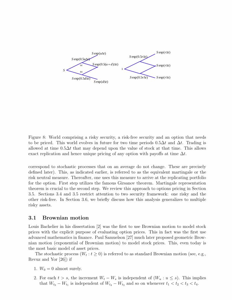
Another way to incorporate three scenarios is to increase the number of time periods tothree. This is illustrated in Figure 8. The two securities are now observed at times zero,0.5∆t and ∆t. At times zero and at 0.5∆t, the stock price can either go up by amountexp(0.5u∆t) or down by amount exp(0.5d∆t) in the next 0.5∆t time. At time ∆t, the stockprice can take three values. In addition, trading is allowed at time 0.5∆t that may dependupon the value of stock at that time. This additional flexibility allows replication of anyoption with payoffs at time ∆t that are a function of the stock price at that time (moregenerally, the payoff could be a function of the path followed by the stock price till time∆t). To see this, one can repeat the argument for the two-security-two scenario-two-time-period case to determine how much money is needed at node (a) in Figure 8 to replicatethe option pay-off at time ∆t. Similarly, one can determine the money needed at node (b).Using these two values, one can determine the amount needed at time zero to construct areplicating portfolio that exactly replicates the option payoff along every scenario at time∆t. This argument easily generalizes to arbitrary n time periods (see Hull [16], Shreve[29]). Cox, Ross and Rubinstein (1979) analyze this as n goes to infinity and show that theresultant risky security price process converges to geometric Brownian motion (exponential

10

S

Risky security Risk free security

exp(u1Dt)

exp(u2Dt)

exp(u3Dt)

1

exp(rDt)

exp(rDt)

exp(rDt)

??

Option payoff

Cu1

Cu2

Cu3

Figure 7: World comprising a risky security, a risk-free security and an option that needsto be priced. This world evolves in future for one time period where the risky security andthe option can take three possible values. No arbitrage principle typically does not providea unique price for the option in this case.

of Brownian motion; Brownian motion is discussed in section 3), a natural setting for morerealistic analysis.

3 Continuous Time Models

We now discuss the European option pricing problem in the continuous-time-continuous-statesettings which has emerged as the primary regime for modeling security prices. As discussedearlier, the key idea is to create a dynamic portfolio that through continuous trading in theunderlying securities up to the option time to maturity, exactly replicates the option payoffin every possible scenario. In this presentation we de-emphasize technicalities to maintainfocus on the key concepts used for pricing options and to keep the discussion accessible toa broad audience. We refer the reader to Shreve [30], Duffie [8], Steele [31] for simple andengaging account of stochastic analysis for derivatives pricing; Also see, [11]).

First in Section 3.1, we briefly introduce Brownian motion, perhaps the most fundamentalcontinuous time stochastic process that is an essential ingredient in modeling security prices.We discuss how this is crucial in driving stochastic differential equations used to modelsecurity prices in Section 3.2. Then in Section 3.3, we briefly review the concepts of stochasticIto integral, quadratic variation and Ito’s formula, necessary to appreciate the stochasticdifferential equation model of security prices. In Section 3.4, we use a well known techniqueto arrive at a replicating portfolio and the Black Scholes partial differential equation foroptions with simple payoff structure in a two security set-up.

Modern approach to options pricing relies on two broad steps: First we determine aprobability measure under which discounted security prices are martingales (martingales

11

)5.0exp( tuS

S1

)5.0exp( tdS

)exp( tuS

)exp( tdS

))(5.0exp( tduS

)5.0exp( trS

)5.0exp( trS

)exp( trS

)exp( trS

)exp( trS

(a)

(b)

Figure 8: World comprising a risky security, a risk-free security and an option that needsto be priced. This world evolves in future for two time periods 0.5∆t and ∆t. Trading isallowed at time 0.5∆t that may depend upon the value of stock at that time. This allowsexact replication and hence unique pricing of any option with payoffs at time ∆t.

correspond to stochastic processes that on an average do not change. These are preciselydefined later). This, as indicated earlier, is referred to as the equivalent martingale or therisk neutral measure. Thereafter, one uses this measure to arrive at the replicating portfoliofor the option. First step utilizes the famous Girsanov theorem. Martingale representationtheorem is crucial to the second step. We review this approach to options pricing in Section3.5. Sections 3.4 and 3.5 restrict attention to two security framework: one risky and theother risk-free. In Section 3.6, we briefly discuss how this analysis generalizes to multiplerisky assets.

3.1 Brownian motion

Louis Bachelier in his dissertation [2] was the first to use Brownian motion to model stockprices with the explicit purpose of evaluating option prices. This in fact was the first useadvanced mathematics in finance. Paul Samuelson [27] much later proposed geometric Brow-nian motion (exponential of Brownian motion) to model stock prices. This, even today isthe most basic model of asset prices.

The stochastic process (Wt : t ≥ 0) is referred to as standard Brownian motion (see, e.g.,Revuz and Yor [26]) if

1. W0 = 0 almost surely.

2. For each t > s, the increment Wt −Ws is independent of (Wu : u ≤ s). This impliesthat Wt2 −Wt1 is independent of Wt4 −Wt3 and so on whenever t1 < t2 < t3 < t4.

12

3. For each t > s, the increment Wt −Ws has a Gaussian distribution with zero meanand variance t− s.

4. The sample paths of (Wt : t ≥ 0) are continuous almost surely.

Technically speaking, (Wt : t ≥ 0) is defined on a probability space (Ω,F , Ft≥0,P)where Ft≥0 is a filtration of F , that is, an increasing sequence of sub-sigma algebras of F .From an intuitive perspective, Ft denotes the information available at time t. The randomvariable Wt is Ft measurable for each t ( i.e., the process Wtt≥0 is adapted to Ft≥0).Heuristically this means that the value of (Ws : s ≤ t) is known at time t. In this chapterwe take Ft to denote the sigma algebra generated by (Ws : s ≤ t). This has ramificationsfor the martingale representation theorem stated later. In addition, the filtration Ft≥0

satisfies the usual conditions. See, e.g., Karatzas and Shreve [18].The independent increments assumption is crucial to modeling risky security prices as

it captures the efficient market hypothesis on security prices ([14]) , that is, any change insecurity prices is essentially due to arrival of new information (independent of what is knownin past). All past information has already been incorporated in the market price.

3.2 Modeling Security Prices

In our model, the security price process is observed till T > 0, time to maturity of theoption to be priced. In particular, in the Brownian motion defined above the time index isrestricted to [0, T ]. The stock price evolution is modeled as a stochastic process St0≤t≤Tdefined on the probability space (Ω,F , F0≤t≤T ,P) and is assumed to satisfy the stochasticdifferential equation (SDE)

dSt = µtStdt+ σtStdWt, (3)

where µt and σt maybe deterministic functions of (t, St) satisfying technical conditions suchthat a unique solution to this SDE exists (see, e.g., Oksendal [24], Karatzas and Shreve [18],Steele [31] for these conditions and a general introduction to SDEs). In (3), the simplest andpopular case corresponds to both µt and σt being constants.

Note thatSt1+t2−St1

St1denotes the return from the security over the time period [t1, t2].

Equation (3) may be best viewed through its discretized Euler’s approximation at times tand t+ δt:

St+δt − StSt

= µtδt+ σt(Wt+δt −Wt).

This suggests that µt captures the drift in the instantaneous return from the security attime t. Similarly, σt captures the sensitivity to the independent noise Wt+δt −Wt present inthe instantaneous return at time t. Since, µt and σt maybe functions of (t, St), independentof the past security prices, and Brownian motion has independent increments, the processSt0≤t≤T is Markov. Heuristically, this means that, given the asset value Ss at time s, thefuture Sts≤t≤T is independent of the past St0≤t≤s.

Equation (3) is a heuristic differential representation of an SDE. A rigorous representationis given by

St = S0 +

∫ t

0

µsSsds+

∫ t

0

σsSsdWs. (4)

13

Here, while∫ t

0µsSsds is a standard Lebesgue integral defined path by path along the sample

space, the integral∫ t

0σsSsdWs is a stochastic integral known as Ito integral after its inventor

Ito [17]. It fundamentally differs from Lebesgue integral as it can be seen that Brownianmotion does not have bounded variation. We briefly discuss this and related relevant resultsin the subsection below.

3.3 Stochastic Calculus

Here we summarize some useful results related to stochastic integrals that are needed in ourdiscussion. The reader is referred to Karatzas and Shreve [18], Protter [25] and Revuz andYor [26] for a comprehensive and rigorous analysis.

3.3.1 Stochastic integral

Suppose that φ : [0, T ] → < is a bounded continuous function. One can then define its

integral∫ T

0φ(s)dAs w.r.t. to a continuous process (At : 0 ≤ t ≤ T ), of finite first order

variation, as the limit

limn→∞

n−1∑i=0

φ(iT/n)(A(i+1)T/n − AiT/n).

(In our analysis, above and below, for notational simplification we have divided T into nequal intervals. Similar results are true if the intervals are allowed to be unequal with thecaveat that the largest interval shrinks to zero as n→∞.) The above approach to definingintegrals fails when the integration is w.r.t. to Brownian motion (Wt : 0 ≤ t ≤ T ). To seethis informally, note that in

n−1∑i=0

|W(i+1)T/n −WiT/n|

the terms |W(i+1)T/n −WiT/n| are i.i.d. and each is distributed as√T/n times N(0, 1), a

standard Gaussian random variable with mean zero and variance 1. This suggests that, dueto the law of large numbers, this sum is close to

√nTE|N(0, 1)| as n becomes large. Hence,

it diverges almost surely as n → ∞. This makes definition of path by path integral w.r.t.Brownian motion difficult.

Ito defined the stochastic integral∫ T

0φ(s)dWs as a limit in the L2 sense1. Specifically, he

considered adapted random processes (φ(t) : 0 ≤ t ≤ T ) such that

E

∫ T

0

φ(s)2ds <∞.

For such functions, the following Ito’s isometry is easily seen

E

[n−1∑i=0

(φ(iT/n)(W(i+1)T/n −WiT/n)

)2

]= E

(n−1∑i=0

φ(iT/n)2T/n

).

1A sequence of random variables (Xn : n ≥ 1) such that EX2n <∞ for all n is said to converge to random

variable X (all defined on the same probability space) in the L2 sense if limn→∞E(Xn −X)2 = 0.

14

To see this, note that φ is an adapted process, the Brownian motion has independent incre-ments, so that φ(iT/n) is independent of W(i+1)T/n −WiT/n. Therefore, the expectation ofthe cross terms in the expansion of the square on the LHS can be seen to be zero. Further,E[φ(iT/n)2(W(i+1)T/n −WiT/n)2] equals E[φ(iT/n)2]T/n.

This identity plays a fundamental role in defining∫ T

0φ(s)dWs as an L2 limit of the se-

quence of random variables∑n−1

i=0 φ(iT/n)(W(i+1)T/n−WiT/n) (see, e.g. Steele [31], Karatzasand Shreve [18]).

3.3.2 Martingale property and quadratic variation

As is well known, martingales capture the idea of a fair game in gambling and are importantto our analysis. Technically, a stochastic process (Yt : 0 ≤ t ≤ T ) on a probability space(Ω,F , F0≤t≤T ,P) is a martingale if it is adapted to the filtration F0≤t≤T , if E|Yt| <∞for all t, and:

E[Yt|Fs] = Ys

almost surely for all 0 ≤ s < t ≤ T .The process (I(t) : 0 ≤ t ≤ T ),

I(t) =k−1∑i=0

φ(iT/n)(W(i+1)T/n −WiT/n) + φ(kT/n)(Wt −WkT/n)

where k is such that t ∈ [kT/n, (k+ 1)T/n), can be easily seen to be a continuous zero meanmartingale using the key observation that for t1 < t2 < t3,

E[φ(t2)(Wt3 −Wt2)|Ft1 ] = E (E[φ(t2)(Wt3 −Wt2)|Ft2 ]|Ft1)

and this equals zero since

E[φ(t2)(Wt3 −Wt2)|Ft2 ] = φ(t2)E[(Wt3 −Wt2)|Ft2 ] = 0.

Using this it can also be shown that the limiting process (∫ t

0φ(s)dWs : 0 ≤ t ≤ T ) is a zero

mean martingale if (φ(t) : 0 ≤ t ≤ T ) is an adapted process and

E

∫ T

0

φ(s)2ds <∞.

Quadratic variation of any process (Xt : 0 ≤ t ≤ T ) may be defined as the L2 limit of

the sequence∑n−1

i=0 (X(i+1)T/n−XiT/n)2 when it exists. This can be seen to equal∫ T

0φ(s)2ds

for the process (∫ t

0φ(s)dWs : 0 ≤ t ≤ T ). In particular the quadratic variation of (Wt : 0 ≤

t ≤ T ) equals a constant T .

3.3.3 Ito’s formula

Ito’s formula provides a key identity that highlights the difference between Ito’s integraland ordinary integral. It is the main tool for analysis of stochastic integrals. Suppose that

15

f : < → < is twice continuously differentiable and E∫ t

0f ′(Ws)

2ds <∞. Then, Ito’s formulastates that

f(Wt) = f(W0) +

∫ t

0

f ′(Ws)dWs +1

2

∫ t

0

f ′′(Ws)ds. (5)

Note that in integration with respect to processes with finite first order variation, the cor-rection term 1

2

∫ t0f ′′(Ws)ds would be absent.

To see why this identity holds, re-express f(Wt)− f(W0) as

n−1∑i=0

(f(W(i+1)t/n)− f(Wit/n)

).

Expanding the summands using the Taylor series expansion and ignoring the remainderterms, we have

n−1∑i=0

f ′(Wit/n)(W(i+1)t/n −Wit/n) +1

2

n−1∑i=0

f ′′(Wit/n)(W(i+1)t/n −Wit/n)2.

The first term converges to∫ t

0f ′(Ws)dWs in L2 as n → ∞. To see that the second term

converges to 12

∫ t0f ′′(Ws)ds it suffices to note that

n−1∑i=0

f ′′(Wit/n)((W(i+1)t/n −Wit/n)2 − t/n

)(6)

converges to zero as n→∞. This is easily seen when |f ′′| is bounded as then (6) is boundedfrom above by

supx|f ′′(x)|

n−1∑i=0

((W(i+1)t/n −Wit/n)2 − t/n

).

The sum above converges to zero in L2 as the quadratic variation of (W (s) : 0 ≤ s ≤ t)equals t.

In the heuristic differential form (5) may be expressed as

df(Wt) = f ′(Wt)dWt +1

2f ′′(Wt)dt.

This form is usually more convenient to manipulate and correctly derive other equations andis preferred to the rigorous representation.

Similarly, for f : [0, T ]× < → < with continuous partial derivatives of second order, wecan show that

df(t,Wt) = ft(t,Wt)dt+ fx(t,Wt)dWt +1

2fxx(t,Wt)dt (7)

where ft denotes the partial derivative w.r.t. the first argument of f(·, ·) and fx and fxxdenote the first and the second order partial derivatives with respect to its second argument.Again, the rigorous representation for (8) is

f(t,Wt) = f(0,W0) +

∫ t

0

ft(s,Ws)ds+

∫ t

0

fx(s,Ws)dWs +1

2

∫ t

0

fxx(s,Ws)ds.

16

3.3.4 Ito processes

The process (Xt : 0 ≤ t ≤ T ) of the (differential) form

dXt = αtdt+ βtdWt

where (αt : 0 ≤ t ≤ T ) and (βt : 0 ≤ t ≤ T ) are adapted processes such that E(∫ T

0β2t dt) <∞

and E(∫ T

0|αt|dt) <∞, are referred to as Ito processes. Ito’s formula can be generalized using

essentially similar arguments to show that

df(t,Xt) = ft(t,Xt)dt+ fx(t,Xt)dXt +1

2fxx(t,Xt)σ

2t dt. (8)

3.4 Black Scholes partial differential equation

As in the Binomial setting, here too we consider two securities. The risky security or thestock price process satisfies (3). The money market (Rt : 0 ≤ t ≤ T ) is governed by a shortrate process (rt : 0 ≤ t ≤ T ) and satisfies the differential equation

dRt = rtRtdt

with R0 = 1. Here short rate rt corresponds to instantaneous return on investment in themoney market at time t. In particular, Rs. 1 invested at time zero in the money market equalsRt = exp(

∫ t0rsds) at time t. In general rt may be random and the process (rt : 0 ≤ t ≤ T )

may be adapted to F0≤t≤T , although typically when short time horizons are involved, adeterministic model of short rates is often used. In fact, it is common to assume that rt = r,a constant, so that Rt = exp(rt). In our analysis, we assume that (rt : 0 ≤ t ≤ T ) isdeterministic to obtain considerable simplification.

Now consider the problem of pricing an option in this market that pays a random amounth(ST ) at time T . For instance, for a call option that matures at time T with strike price K,we have h(ST ) = max(ST −K, 0). We now construct a replicating portfolio for this option.Consider the recipe process (bt : 0 ≤ t ≤ T ) for constructing a replicating portfolio. We startwith amount P0. At time t, let Pt denote the value of the portfolio. This is used to purchasebt number of stock (we allow bt to take non-integral values). The remaining amount Pt−btStis invested in the money market. Then, the portfolio process evolves as:

dPt = (Pt − btSt)rtdt+ btdSt. (9)

Due to the Markov nature of the stock price process, and since the option payoff is afunction of ST , at time t, the option price can be seen to be a function of t and St. Denotethis price by c(t, St). By Ito’s formula (8), (assuming c(·, ·) is sufficiently smooth):

dc(t, St) = ct(t, St)dt+ cx(t, St)dSt +1

2cxx(t, St)σ

2t dt,

with c(T, ST ) = h(ST ). This maybe e-expressed as:

dc(t, St) =

(ct(t, St) + cx(t, St)Stµt +

1

2cxx(t, St)σ

2tS

2t

)dt+ cx(t, St)σtStdWt (10)

17

Our aim is to select (bt : 0 ≤ t ≤ T ) so that Pt equals c(t, St) for all (t, St). To this end, (9)can be re-expressed as

dPt = ((Pt − btSt)rt + btµtSt) dt+ btσtStdWt. (11)

To make Pt = c(t, St) we equate the drift (terms corresponding to dt) as well as the diffusionterms (terms corresponding to dWt) in (10) and (11). This requires that bt = cx(t, St) and

ct(t, St) +1

2cxx(t, St)S

2t σ

2t − c(t, St)rt + cx(t, St)Strt = 0.

The above should hold for all values of St ≥ 0. This specifies the famous Black-Scholespartial differential equation (pde) satisfied by the option price process:

ct(t, x) + cx(t, x)xrt +1

2cxx(t, x)x2σ2

t − c(t, x)rt = 0 (12)

for 0 ≤ t ≤ T , x ≥ 0 and the the boundary condition c(T, x) = h(x) for all x.This is a parabolic pde that can be solved for the price process c(t, x) for all t ∈ [0, T )

and x ≥ 0. Once this is available, the replicating portfolio process is constructed as follows.P0 = c(0, S0) denotes the initial amount needed. This is also the value of the option at timezero. At this time cx(0, S0) number of risky security is purchased and the remaining amountc(0, S0)− cx(0, S0)S0 is invested in the money market. At any time t, the number of stocksheld is adjusted to cx(t, St). Then, the value of the portfolio equals c(t, St). The amountc(t, St) − cx(t, St)St is invested in the money market. These adjustments are made at eachtime t ∈ [0, T ). At time T then the portfolio value equals c(T, ST ) = h(ST ) so that theoption is perfectly replicated.

3.5 Equivalent martingale measure

As in the discrete case, in the continuous setting as well, under mild technical conditions,there exists another probability measure referred to as the risk neutral measure or the equiv-alent martingale measure under which the discounted stock price process is a martingale.This then makes the discounted replicating portfolio process a martingale, which in turnensures that if an option can be replicated, then the discounted option price process is amartingale. The importance of this result is that it brings to bear the well developed andelegant theory of martingales to derivative pricing leading to deep insights into derivativespricing and hedging (see Harrison and Kreps [12] and Harrison and Pliska [13] for seminalpapers on this approach).

Martingale representation theorem and Girsanov theorem are two fundamental resultsfrom probability that are essential to this approach. We state them in a simple one dimen-sional setting.

Martingale Representation Theorem: If the stochastic process (Mt : 0 ≤ t ≤ T ) definedon (Ω,F , F0≤t≤T ,P) is a martingale, then there exists an adapted process (ν(t) : 0 ≤ t ≤T ) such that E(

∫ T0ν(t)2dt) <∞ and

Mt = M0 +

∫ t

0

ν(s)dWs

18

for 0 ≤ t ≤ T .As noted earlier, under mild conditions a stochastic integral process is a martingale. The

above theorem states that the converse is also true. That is, on this probability space, everymartingale is a stochastic integral.

Some preliminaries to help state the Girsanov theorem: Two probability measures P andP∗ defined on the same space are said to be equivalent if they assign positive probability tosame sets. Equivalently, they assign zero probability to same sets. Further if P and P∗ areequivalent probability measures, then there exists an almost surely positive Radon-Nikodymderivative of P∗ w.r.t. P , call it Y , such that P∗(A) = EPY I(A) (here, the subscript onE denotes that the expectation is with respect to probability measure P and I(·) is anindicator function). Furthermore, if Z is a strictly positive random variable almost surelywith EPZ = 1 then the set function Q(A) = EPZI(A) can be seen to be a probabilitymeasure that is equivalent to P . Girsanov Theorem specifies the new distribution of theBrownian motion (Wt : 0 ≤ t ≤ T ) under probability measures equivalent to P . Specifically,consider the process

Yt = exp

(∫ t

0

νsdWs −1

2

∫ t

0

ν2sds

).

Let Xt =∫ t

0νsdWs − 1

2

∫ t0ν2sds. Then Yt = exp(Xt) so that using Ito’s formula

dYt = YtνtdWt,

or in its meaningful form

Yt = 1 +

∫ t

0

YsνsdWs.

Under technical conditions the stochastic integral is a mean zero martingale so that (Yt :0 ≤ t ≤ T ) is a positive mean 1 martingale. Let Pν(A) = EP [YT I(A)].

Girsanov Theorem: Under the probability measure Pν , under technical conditions on(νt : 0 ≤ t ≤ T ), the process (W ν

t : 0 ≤ t ≤ T ) where

W νt = Wt −

∫ t

0

νsds

(or dW νt = dWt − νtdt in the differential notation) is a standard Brownian motion. Equiva-

lently, (Wt : 0 ≤ t ≤ T ) is a standard Brownian motion plus the drift process (∫ t

0νsds : 0 ≤

t ≤ T ).

3.5.1 Identifying the equivalent martingale measure

Armed with the above two powerful results we can now return to the process of finding theequivalent martingale measure for the stock price process and the replicating portfolio forthe option price process. Recall that the stock price follows the SDE

dSt = µtStdt+ σtStdWt.

We now allow this to be a general Ito process, that is, µt and σt are adapted processes(not just deterministic functions of t and St). The option payoff H is allowed to be an FT

19

measurable random variable. This means that it can be a function of (St : 0 ≤ t ≤ T ), notjust of ST .

Note that R−1t St has the form f(t, St) where St is an Ito’s process. Therefore, using the

Ito’s formula, the discounted stock price process satisfies the relation

d(R−1t St) = −rtR−1

t St +R−1t dSt = R−1

t St ((µt − rt)dt+ σtdWt) . (13)

It is now easy to see from Girsanov theorem that if σt > 0 almost surely, then underthe probability measure Pν with νt = rt−µt

σtthe discounted stock price process satisfies the

relationd(R−1

t St) = R−1t StσtdW

νt

(this can be seen by replacing dWt by dW νt + νtdt in (13). This operation in differential no-

tation can be shown to be technically valid). This being a stochastic integral is a martingale(modulo technical conditions), so that Pν is the equivalent martingale measure.

It is easy to see by applying the Ito’s formula (Note that St = RtXt where Xt = R−1t St

satisfies the SDE above) that

dSt = rtStdt+ StσtdWνt . (14)

Hence, under the equivalent martingale measure Pν , the drift of the stock price processchanges from µt to rt. Therefore, Pν is also referred to as the risk neutral measure.

3.5.2 Creating the replicating portfolio process

Now consider the problem of creating the replicating process for an option with pay-off H.Define Vt for 0 ≤ t ≤ T so that

R−1t Vt = EPν [R

−1T H|Ft].

Note that VT = H.Our plan is to construct a replicating portfolio process (Pt : 0 ≤ t ≤ T ) such that Pt = Vt

for all t. Then, since PT = H we have replicated the option with this portfolio process andPt then denotes the price of the option at time t, i.e.,

Pt = EPν

[exp

(−∫ T

t

rsds

)H|Ft

]. (15)

Then, the option price is simply the conditional expectation of the discounted option payoffunder the risk neutral or the equivalent martingale measure.

To this end, it is easily seen from the law of iterated conditional expectations that fors < t,

R−1s Vs = EPν

(EPν [R

−1T VT |Ft]|Fs

)= EPν [R

−1t Vt|Fs],

that is, (R−1t Vt : 0 ≤ t ≤ T ) is a martingale. From the martingale representation theorem

there exists an adapted process (wt : 0 ≤ t ≤ T ) such that

d(R−1t Vt) = wtdW

νt . (16)

20

Now consider a portfolio process (Pt : 0 ≤ t ≤ T ) with the associated recipe process(bt : 0 ≤ t ≤ T ). Recall that this means that we start with wealth P0. At any time t theportfolio value is denoted by Pt which is used to purchase bt units of stock. The remainingamount Pt − btSt is invested in the money market. Then, the portfolio process evolves as in(9). The discounted portfolio process

d(R−1t Pt) = R−1

t btSt ((µt − rt)dt+ σtdWt) = R−1t btStσtdW

νt . (17)

Therefore, under technical conditions, the discounted portfolio process being a stochasticintegral, is a martingale under Pν .

From (16) and (17) its clear that if we set P0 = V0 and bt = wtRtStσt

then Pt = Vt for allt. In particular we have constructed a replicating portfolio. In particular, under technicalconditions, primarily that σt > 0 almost surely, for almost every t every option can bereplicated so that this market is complete.

3.5.3 Black Scholes pricing

Suppose that the stock price follows the SDE

dSt = µStdt+ σStdWt

where µ and σ > 0 are constant. Furthermore the short rate rt equals a constant r. Fromabove and (14), it follows that under the equivalent martingale measure Pν

dSt = rStdt+ StσdWνt . (18)

Equivalently,St = S0 exp(σW ν

t + (r − σ2/2)t). (19)

The fact that St given by (19) satisfies (18) can be seen applying Ito’s formula to (19). Since(18) has a unique solution, it is given by (19). Since, W ν

t is the standard Brownian motionunder Pν , it follows that St is geometric Brownian motion and that for each t, logSt hasa Gaussian distribution with mean (r − σ2/2)t+ logS0 and variance σ2t.

Now suppose that we want to price a call option that matures at time T and has a strikeprice K. Then, H = (ST −K)+ (note that (x)+ = max(x, 0)). The option price equals

E([exp

(N((r − σ2/2)T + logS0, σ

2T ))−K

]+(20)

where N(a, b) denotes a Gaussian distributed random variable with mean a and variance b.(20) can be easily evaluated to give the price of the European call option. The option priceat time t can be inferred from (15) to equal

E([exp

(N((r − σ2/2)(T − t) + logSt, σ

2(T − t)))−K

]+.

Call this c(t, St). It can be shown that this function satisfies the Black Scholes pde (12) withh(x) = (x−K)+.

21

3.6 Multiple assets

Now we extend the analysis to n risky assets or stocks driven by n independent sources ofnoise modeled by independent Brownian motions (W 1

t , . . . ,Wnt : 0 ≤ t ≤ T ). Specifically,

we assume that n assets (S1t , . . . , S

nt : 0 ≤ t ≤ T ) satisfy the SDE

dSit = µitSitdt+

n∑j=1

σijt SitdW

jt (21)

for i = 1, . . . , n. Here we assume that each µi and σij is an adapted process and satisfyrestrictions so that the integrals associated with (21) are well defined. In addition we letRt = exp(

∫ t0r(s)ds) as before. Above, the number of Brownian motions may be taken to be

different from the number of securities, however the results are more elegant when the twoare equal. This is also a popular assumption in practice.

The key observation from essentially repeating the analysis as for the single risky assetis that for the equivalent martingale measure to exist, the matrix σijt has to be invertiblealmost everywhere. This condition is also essential to create a replicating portfolio for anygiven option (that is, for the market to be complete).

It is easy to see that

dR−1t Sit = Sit

((µit − rt)dt+

n∑j=1

σijt dWjt

)

for all i. Now we look for conditions under which the equivalent martingale measure exists.Using the Girsanov theorem, it can be shown that if Pν is equivalent to P then, under it,

dW ν,jt = dW j

t − νjt dt

for each j, are independent standard Brownian motions for some adapted processes (νj : j ≤n). Hence, for Pν to be an equivalent martingale measure (so that each discounted securityprocess is a martingale under it) a necessary condition is

µit − rt =n∑j=1

σijt νj

for each i everywhere except possibly on a set of measure zero. This means that the matrixσijt has to be invertible everywhere except possibly on a set of measure zero.

Similarly, given an option with payoff H, we now look for a replicating portfolio processunder the assumption that equivalent martingale measure Pν exists. Consider a portfolioprocess (Pt : 0 ≤ t ≤ T ) that at any time t purchases bit number of security i. The remainingwealth Pt −

∑n1 b

itS

it is invested in the money market. Hence,

dPt =

((Pt −

n∑1

bitSit)rt +

n∑1

bitµitS

it

)dt+

n∑i=1

bitSit

n∑j=1

σijt dWjt (22)

22

and

dR−1t Pt = R−1

t

n∑i=1

bitSit

n∑j=1

σijt dWν,jt .

Since this is a stochastic integral, under mild technical conditions it is a martingale.Again, since the equivalent martingale measure Pν exists we can define Vt for 0 ≤ t ≤ T

so thatR−1t Vt = EPν [R

−1T H|Ft].

Note that VT = H.As before, (R−1

t Vt : 0 ≤ t ≤ T ) is a martingale. Then, from a multi-dimensional version ofthe martingale representation theorem (see any standard text, e.g., Steele [31]), the existenceof an adapted process (wt ∈ <n : 0 ≤ t ≤ T ) can be shown such that

d(R−1t V (t)) =

n∑j=1

wjtdWν,jt . (23)

Then, to be able to replicate the option with portfolio process (Pt : 0 ≤ t ≤ T ) we needthat P0 = V0 and

wjt = R−1t

n∑i=1

bitSitσ

ijt

for each j almost everywhere. This again can be solved for (bt ∈ <n : 0 ≤ t ≤ T ) if thetranspose of the matrix σijt is invertible for almost all t. We refer the reader to standardtexts, e.g., Karatzas and Shreve [19], Duffie [8], Shreve [30], Steele [31] for a comprehensivetreatment of options pricing in the multi-dimensional settings.

4 Conclusion

In this chapter we introduced derivatives pricing theory emphasizing its history and itsimportance to modern finance. We discussed some popular derivatives. we also describedthe no-arbitrage based pricing methodology, first in the simple binomial tree setting andthen for continuous time models.

References

[1] B. E. Baaquie, Interest Rate and Coupon Bonds in Quantum Finance, (2010), Cam-bridge.

[2] L. Bachelier, Theorie de la Speculation, (1900), Gauthier-Villars.

[3] F. Black and M. Scholes, The Pricing of Options and Corporate Liabilities, Journalof Political Economy 81 (3) (1973), 637-654.

[4] D. Brigo and F. Mercurio, Interest Rate Models: Theory and Practice: with Smile,Inflation, and Credit, (2006), Springer Verlag.

23

[5] A. J. G. Cairns, Interest Rate Models, (2004), Princeton University Press.

[6] J. Y. Cambell, A. W. Lo and A. C. Mackinlay, The Econometrics of Financial Mar-kets, (2006), Princeton University Press.

[7] J. C. Cox, S. A. Ross and M. Rubinstein. Option Pricing: A Simplified Approach,Journal of Financial Economics 7, (1979), 229–263.

[8] D. Duffie, Dyanamic Asset Pricing Theory, (1996), Princeton University Press.

[9] D. Duffie, How Big Banks Fail: and What To Do About It, (2010), Princeton Univer-sity Press.

[10] D. Duffie and K. Singleton, Credit Risk: Pricing, Measurement, and Management,(2003), Princeton University Press.

[11] J. P. Fouque, G. Papanicolaou, K. R. Sircar, Derivatives in Financial Markets withStochastic Volatility, (2000), Cambridge University Press.

[12] J. M. Harrison and D. Kreps, Martingales and Arbitrage in Multiperiod Security Mar-kets, Journal of Economic Theory, 20, (1979), 381–408.

[13] J. M. Harrison and S. R. Pliska, Martingales and Stochastic Integrals in the Theoryof Continuous Trading, Stochastic Processes and Applications, 11, (1981), 215–260.

[14] E. F. Fama, Efficient Capital Markets: A Review of Theory and Empirical Work,Journal of Finance, 25, 2, (1970).

[15] P. Glasserman, Monte Carlo Methods in Financial Engineering, (2003), Springer-Verlag, New York.

[16] J. C. Hull, Options, Futures and Other Derivative Securities, Seventh Edition, (2008),Prentice Hall.

[17] K. Ito, On a Stochastic Integral Equation, Proc. Imperial Academy Tokyo, 22, (1946),32–35.

[18] I. Karatzas and S. Shreve, Brownian Motion and Stochastic Calculus, (1991) Springer,New York.

[19] I. Karatzas and S. Shreve, Methods of Mathematical Finance, (1998) Springer, NewYork.

[20] D. Lando, Credit Risk Modeling, (2005), New Age International Publishers.

[21] M. Magill and M. Quinzii, Theory of Incomplete Markets, Volume 1, (2002), MITPress.

[22] A. J. McNeil, R. Frey and P. Embrechts, Quantitative Risk Management: Concepts,Techniques, and Tools, (2005) Princeton University Press

24

[23] A. Meucci, Risk and Asset Allocation, (2005), Springer.

[24] B. Oksendal, Stochastic Differential Equations: An Introduction with Applications,5th ed. (1998) Springer, New York.

[25] P. Protter, Stochastic Integration and Differential Equations: A New Approach,(1990), Springer-Verlag.

[26] D. Revuz and M. Yor, Continuous Martingales and Brownian motion, 3rd Ed., (1999),Springer-Verlag.

[27] P. Samuelson, Rational Theory of Warrant Pricing, Industrial Management Review,6, 2, (1965), 13–31.

[28] P. J. Schonbucher, Credit Derivative Pricing Models, (2003), Wiley.

[29] S. E. Shreve, Stochastic Calculus for Finance I: The Binomial Asset Pricing Model,(2004), Springer.

[30] S. E. Shreve, Stochastic Calculus for Finance II: Continuous-Time Models (2004),Springer.

[31] J. M. Steele, Stochastic Calculus and Financial Applications, (2001), Springer.

25