An Introduction to Factor Graphs - Bioinformatics...

MLSB 2008, Copenhagen 1

An Introduction to Factor Graphs

Hans-Andrea Loeliger

2

Definition

A factor graph represents the factorization of a function of severalvariables. We use Forney-style factor graphs (Forney, 2001).

Example:

f (x1, x2, x3, x4, x5) = fA(x1, x2, x3) · fB(x3, x4, x5) · fC(x4).

x1

fA

x2

x3

fB

fC

x4

x5

Rules:

• A node for every factor.

• An edge or half-edge for every variable.

• Node g is connected to edge x iff variable x appears in factor g.

(What if some variable appears in more than 2 factors?)

3

Example:

Markov Chain

pXY Z(x, y, z) = pX(x) pY |X(y|x) pZ|Y (z|y).

pX

X

pY |X

Y

pZ|Y

Z

We will often use capital letters for the variables. (Why?)

Further examples will come later.

4

Message Passing Algorithms

operate by passing messages along the edges of a factor graph:

-

�

6?

6?

-

�

-

�

6?

6?

-

�

-

� . . .

-

�

6?

-

�

6?

-

�

5

A main point of factor graphs (and similar graphical notations):

A Unified View of Historically Different Things

Statistical physics:- Markov random fields (Ising 1925)

Signal processing:- linear state-space models and Kalman filtering: Kalman 1960. . .- recursive least-squares adaptive filters- Hidden Markov models: Baum et al. 1966. . .- unification: Levy et al. 1996. . .

Error correcting codes:- Low-density parity check codes: Gallager 1962; Tanner 1981;MacKay 1996; Luby et al. 1998. . .- Convolutional codes and Viterbi decoding: Forney 1973. . .- Turbo codes: Berrou et al. 1993. . .

Machine learning, statistics:- Bayesian networks: Pearl 1988; Shachter 1988; Lauritzen andSpiegelhalter 1988; Shafer and Shenoy 1990. . .

6

Other Notation Systems for Graphical Models

Example: p(u, w, x, y, z) = p(u)p(w)p(x|u, w)p(y|x)p(z|x).

WU

X =

Y

Z

Forney-style factor graph.

� ��W

� ��U

� ��X

� ��Y

� ��Z

Original factor graph [FKLW 1997].

� ��W - � ��X

� ��U

?

?

� ��Y

- � ��Z

Bayesian network.

� ��W � ��X�

��

��

� ��U

� ��Y

� ��Z

Markov random field.

7

Outline

1. Introduction

2. The sum-product and max-product algorithms

3. More about factor graphs

4. Applications of sum-product & max-productto hidden Markov models

5. Graphs with cycles, continuous variables, . . .

8

The Two Basic Problems

1. Marginalization: Compute

fk(xk)4=

∑x1, . . . , xn

except xk

f (x1, . . . , xn)

2. Maximization: Compute the “max-marginal”

fk(xk)4= max

x1, . . . , xn

except xk

f (x1, . . . , xn)

assuming that f is real-valued and nonnegative and has a maximum.Note that

argmax f (x1, . . . , xn) =(argmax f1(x1), . . . , argmax fn(xn)

).

For large n, both problems are in general intractableeven for x1, . . . , xn ∈ {0, 1}.

9

Factorization Helps

For example, if f (x1, . . . , fn) = f1(x1)f2(x2) · · · fn(xn) then

fk(xk) =

(∑x1

f1(x1)

)· · ·(∑

xk−1

fk−1(xk−1)

)fk(xk) · · ·

(∑xn

fn(xn)

)and

fk(xk) =

(max

x1

f1(x1)

)· · ·(

maxxk−1

fk−1(xk−1)

)fk(xk) · · ·

(max

xnfn(xn)

).

Factorization helps also beyond this trivial example.

10

Towards the sum-product algorithm:

Computing Marginals—A Generic Example

Assume we wish to compute

f3(x3) =∑

x1, . . . , x7

except x3

f (x1, . . . , x7)

and assume that f can be factored as follows:

f1

X1

f2

X2

f3

X3

f4

X4

f5

X5

f7

X7

f6

X6

11

Example cont’d:

Closing Boxes by the Distributive Law

f1

X1

f2

X2

f3

X3

f4

X4

f5

X5

f7

X7

f6

X6

f3(x3) =

(∑x1,x2

f1(x1)f2(x2)f3(x1, x2, x3)

)

·

(∑x4,x5

f4(x4)f5(x3, x4, x5)

(∑x6,x7

f6(x5, x6, x7)f7(x7)

))

12

Example cont’d: Message Passing View

f1

X1

f2

X2

f3

X3- �

f4

X4

f5

X5�

f7

X7

f6

X6

f3(x3) =

(∑x1,x2

f1(x1)f2(x2)f3(x1, x2, x3)︸︷︷︸−→µX3

(x3)

)

·

(∑x4,x5

f4(x4)f5(x3, x4, x5)

(∑x6,x7

f6(x5, x6, x7)f7(x7)︸︷︷︸←−µX5

(x5)

)︸︷︷︸

←−µX3(x3)

)

13

Example cont’d: Messages Everywhere

f1

X1-

f2

X2?

f3

X3- �

f4

X4 ?

f5

X5�

f7

X7 ?

f6

X6

With −→µX1(x1)4= f1(x1),

−→µX2(x2)4= f2(x2), etc., we have

−→µX3(x3) =∑x1,x2

−→µX1(x1)−→µX2(x2)f3(x1, x2, x3)

←−µX5(x5) =∑x6,x7

−→µX7(x7)f6(x5, x6, x7)

←−µX3(x3) =∑x4,x5

−→µX4(x4)←−µX5(x5)f5(x3, x4, x5)

14

The Sum-Product Algorithm (Belief Propagation)

HHHH

HHH

Y1

..

.

��

Yn

gXH

HHj

��* - �

Sum-product message computation rule:

−→µX(x) =∑

y1,...,yn

g(x, y1, . . . , yn)−→µY1(y1) · · · −→µYn(yn)

Sum-product theorem:

If the factor graph for some function f has no cycles, then

fX(x) = −→µX(x)←−µX(x).

15

Towards the max-product algorithm:

Computing Max-Marginals—A Generic Example

Assume we wish to compute

f3(x3) = maxx1, . . . , x7

except x3

f (x1, . . . , x7)

and assume that f can be factored as follows:

f1

X1

f2

X2

f3

X3

f4

X4

f5

X5

f7

X7

f6

X6

16

Example:

Closing Boxes by the Distributive Law

f1

X1

f2

X2

f3

X3

f4

X4

f5

X5

f7

X7

f6

X6

f3(x3) =

(maxx1,x2

f1(x1)f2(x2)f3(x1, x2, x3)

)

·

(maxx4,x5

f4(x4)f5(x3, x4, x5)

(maxx6,x7

f6(x5, x6, x7)f7(x7)

))

17

Example cont’d: Message Passing View

f1

X1

f2

X2

f3

X3- �

f4

X4

f5

X5�

f7

X7

f6

X6

f3(x3) =

(maxx1,x2

f1(x1)f2(x2)f3(x1, x2, x3)︸︷︷︸−→µX3

(x3)

)

·

(maxx4,x5

f4(x4)f5(x3, x4, x5)

(maxx6,x7

f6(x5, x6, x7)f7(x7)︸︷︷︸←−µX5

(x5)

)︸︷︷︸

←−µX3(x3)

)

18

Example cont’d: Messages Everywhere

f1

X1-

f2

X2?

f3

X3- �

f4

X4 ?

f5

X5�

f7

X7 ?

f6

X6

With −→µX1(x1)4= f1(x1),

−→µX2(x2)4= f2(x2), etc., we have

−→µX3(x3) = maxx1,x2

−→µX1(x1)−→µX2(x2)f3(x1, x2, x3)

←−µX5(x5) = maxx6,x7

−→µX7(x7)f6(x5, x6, x7)

←−µX3(x3) = maxx4,x5

−→µX4(x4)←−µX5(x5)f5(x3, x4, x5)

19

The Max-Product Algorithm

HHHHH

HH

Y1

..

.

��

��

Yn

gXHHHj

��* - �

Max-product message computation rule:

−→µX(x) = maxy1,...,yn

g(x, y1, . . . , yn)−→µY1(y1) · · · −→µYn(yn)

Max-product theorem:

If the factor graph for some global function f has no cycles, then

fX(x) = −→µX(x)←−µX(x).

20

Outline

1. Introduction





21

Terminology

x1

fA

x2

x3

fB

fC

x4

x5

Global function f = product of all factors; usually (but not always!)real and nonnegative.

A configuration is an assignment of values to all variables.

The configuration space is the set of all configurations, which is thedomain of the global function.

A configuration ω = (x1, . . . , x5) is valid iff f (ω) 6= 0.

22

Invalid Configurations Do Not Affect Marginals

A configuration ω = (x1, . . . , xn) is valid iff f (ω) 6= 0.

Recall:

1. Marginalization: Compute

fk(xk)4=

∑x1, . . . , xn

except xk

f (x1, . . . , xn)

2. Maximization: Compute the “max-marginal”

fk(xk)4= max

x1, . . . , xn

except xk

f (x1, . . . , xn)

assuming that f is real-valued and nonnegative and has a maximum.

Constraints may be expressed by factors that evaluate to 0 if theconstraint is violated.

23

Branching Point = Equality Constraint Factor

X

X ′

= X ′′ ⇐⇒ X t

The factor

f=(x, x′, x′′)4=

{1, if x = x′ = x′′

0, else

enforces X = X ′ = X ′′ for every valid configuration.

More general:

f=(x, x′, x′′)4= δ(x− x′)δ(x− x′′)

where δ denotes the Kronecker delta for discrete variables and theDirac delta for discrete variables.

24

Example:

Independent Observations

Let Y1 and Y2 be two independent observations of X:

p(x, y1, y2) = p(x)p(y1|x)p(y2|x).

pX

X

=

pY1|X

Y1

pY2|X

Y2

Literally, the factor graph represents an extended model

p(x, x′, x′′, y1, y2) = p(x)p(y1|x′)p(y2|x′′)f=(x, x′, x′′)

with the same marginals and max-marginals as p(x, y1, y2).

25

From A Priori to A Posteriori Probability

Example (cont’d): Let Y1 = y1 and Y2 = y2 be two independentobservations of X, i.e., p(x, y1, y2) = p(x)p(y1|x)p(y2|x).

For fixed y1 and y2, we have

p(x|y1, y2) =p(x, y1, y2)

p(y1, y2)∝ p(x, y1, y2).

pX

X

=

pY1|X

y1

pY2|X

y2

The factorization is unchanged (except for a scale factor).

Known variables will be denoted by small letters;unknown variables will usually be denoted by capital letters.

26

Outline

1. Introduction





28

Sum-product algorithm applied to HMM:

Estimation of Current State

p(xn|y1, . . . , yn) =p(xn, y1, . . . , yn)

p(y1, . . . , yn)

∝ p(xn, y1, . . . , yn)

=∑x0

. . .∑xn−1

p(x0, x1, . . . , xn, y1, y2, . . . , yn)

= −→µXn(xn).

For n = 2:

-X0

- =

?

6

?

y1

--

-X1

- =

?

6

?

y2

--

-X2

- =

?

6=1

?

Y3

-�

=1. . .

29

Backward Message in Chain Rule Model

pX

-X

�

pY |X

-Y

If Y = y is known (observed):

←−µX(x) = pY |X(y|x),

the likelihood function.

If Y is unknown:

←−µX(x) =∑

y

pY |X(y|x)

= 1.

30


Prediction of Next Output Symbol

p(yn+1|y1, . . . , yn) =p(y1, . . . , yn+1)

p(y1, . . . , yn)∝ p(y1, . . . , yn+1)

=∑

x0,x1,...,xn

p(x0, x1, . . . , xn, y1, y2, . . . , yn, yn+1)

= −→µYn(yn).

For n = 2:

-X0

- =

?

6

?

y1

--

-X1

- =

?

6

?

y2

--

-X2

- =

?

?

?

Y3?

-�

=1. . .

31


Estimation of Time-k State

p(xk | y1, y2, . . . , yn) =p(xk, y1, y2, . . . , yn)

p(y1, y2, . . . , yn)∝ p(xk, y1, y2, . . . , yn)

=∑

x0, . . . , xn

except xk

p(x0, x1, . . . , xn, y1, y2, . . . , yn)

= −→µXk(xk)←−µXk

(xk)

For k = 1:

-X0

- =

?

6

?

y1

--

-X1

-�

=

?

6

?

y2

-�

-X2� =

?

6

?

y3

-� . . .

32


All States Simultaneously

p(xk|y1, . . . , yn) for all k:

-X0

-�

=

?

6

?

y1

--

�

-X1

-�

=

?

6

?

y2

--

�

-X2

-�

=

?

6

?

y3

-�

- . . .

In this application, the sum-product algorithm coincides with theBaum-Welch / BCJR forward-backward algorithm.

33

Scaling of Messages

In all the examples so far:

• The final result (such as −→µXk(xk)←−µXk

(xk)) equals the desiredquantity (such as p(xk|y1, . . . , yn)) only up to a scale factor.

• The missing scale factor γ may be recovered at the end fromthe condition ∑

xk

γ−→µXk(xk)←−µXk

(xk) = 1.

• It follows that messages may be scaled freely along the way.

• Such message scaling is often mandatory to avoid numericalproblems.

34


Probability of the Observation

p(y1, . . . , yn) =∑x0

. . .∑xn

p(x0, x1, . . . , xn, y1, y2, . . . , yn)

=∑xn

−→µXn(xn).

This is a number. Scale factors cannot be neglected in this case.

For n = 2:

-X0

- =

?

6

?

y1

--

-X1

- =

?

6

?

y2

--

-X2

- =

?

6=1

?

Y3

-�

=1. . .

35

Max-product algorithm applied to HMM:

MAP Estimate of the State Trajectory

The estimate

(x0, . . . , xn)MAP = argmaxx0,...,xn

p(x0, . . . , xn|y1, . . . , yn)

= argmaxx0,...,xn

p(x0, . . . , xn, y1, . . . , yn)

may be obtained by computing

pk(xk)4= max

x1, . . . , xn

except xk

p(x0, . . . , xn, y1, . . . , yn)


(xk)

for all k by forward-backward max-product sweeps.

In this example, the max-product algorithm is a time-symmetricversion of the Viterbi algorithm with soft output.

36

Max-product algorithm applied to HMM:

MAP Estimate of the State Trajectory cont’d

Computing

pk(xk)4= max

x1, . . . , xn

except xk

p(x0, . . . , xn, y1, . . . , yn)


(xk)

simultaneously for all k:

-X0

-�

=

?

6

?

y1

--

�

-X1

-�

=

?

6

?

y2

--

�

-X2

-�

=

?

6

?

y3

-�

- . . .

37

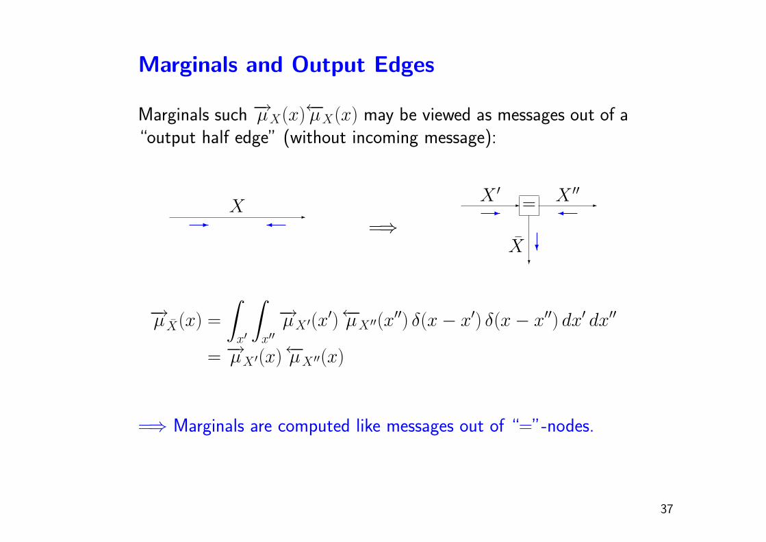
Marginals and Output Edges

Marginals such −→µX(x)←−µX(x) may be viewed as messages out of a“output half edge” (without incoming message):

-X

- � =⇒-

X ′- = -

X ′′�

?

X ?

−→µ X(x) =

∫x′

∫x′′

−→µX ′(x′)←−µX ′′(x

′′) δ(x− x′) δ(x− x′′) dx′ dx′′

= −→µX ′(x)←−µX ′′(x)

=⇒ Marginals are computed like messages out of “=”-nodes.

38

Outline

1. Introduction





39

Factor Graphs with Cycles? Continuous Variables?

-

�

6?

6?

-

�

-

�

6?

6?

-

�

-

�

-

�

6?

-

�

6?

-

�

40

Example:

Error Correcting Codes (e.g. LDPC Codes)

Codeword x = (x1, . . . , xn) ∈ C ⊂ {0, 1}n. Received y = (y1, . . . , yn) ∈ Rn.

p(x, y) ∝ p(y|x)δC(x).f⊕(z1, . . . , zm)

=

{1, if z1 + . . . + zm ≡ 0 mod 2

0, else

code membership function

δC(x) =

{1, if x ∈ C0, else

“random” connections

=LL

��

=\

\��

=\

\LL

��

⊕��

LL\\

⊕�

��

LL

. . .

channel model p(y|x)

e.g., p(y|x) =

n∏`=1

p(y`|x`)

X1

y1

X2

y2

Xn

yn

Decoding by iterative sum-product message passing.

41

Example:

Magnets, Spin Glasses, etc.

Configuration x = (x1, . . . , xn), xk ∈ {0, 1}.

“Energy” w(x) =∑

k

βkxk +∑

neighboring pairs (k, `)

βk,`(xk − x`)2

p(x) ∝ e−w(x) =∏k

e−βkxk∏

neighboring pairs (k, `)

e−βk,`(xk−x`)2

=HH

=HH

=HH

=HH

=HH

=HH

=HH

=HH

=HH

43

Example:

Least-Squares Problems

Minimizingn∑

k=1

x2k subject to (linear or nonlinear) constraints is

equivalent to maximizing

e−∑n

k=1 x2k =

n∏k=1

e−x2k

subject to the given constraints.

constraints

X1

e−x21

. . .Xn

e−x2n

44

General Linear State Space Model

. . .-

Xk−1Ak

-

?

Uk

Bk

?

+ -Xk =

?

Ck

?Yk

-Ak+1-

?

Uk+1

Bk+1

?

+ -Xk+1 =

?

Ck+1

?Yk+1

-

. . .

Xk = AkXk−1 + BkUk

Yk = CkXk

45

Gaussian Message Passing in Linear Models

encompasses much of classical signal processing and appears oftenas a component of more complex problems/algorithms.

Note:

1. Gaussianity of messages is preserved in linear models.

2. Includes Kalman filtering and recursive least-squares algorithms.

3. For Gaussian messages, the sum-product (integral-product) al-gorithm coincides with the max-product algorithm.

4. For jointly Gaussian random variables,MAP estimation = MMSE estimation = LMMSE estimation.

5. Even if X and Y are not jointly Gaussian, the LMMSE estimateof X from Y = y may be obtained by pretending that X and Yare jointly Gaussian (with their actual means and second-ordermoments) and forming the corresponding MAP estimate.

See “The factor graph approach to model-based signal processing,”

Proceedings of the IEEE, June 2007.

46

Continuous Variables: Message Types

The following message types are widely applicable.

• Quantization of messages into discrete bins. Infeasible in higherdimensions.

• Single point: the message µ(x) is replaced by a temporary orfinal estimate x.

• Function value and gradient at a point selected by the receivingnode. Allows steepest-ascent (descent) algorithms.

• Gaussians. Works for Kalman filtering.

• Gaussian mixtures.

• List of samples: a pdf can be represented by a list of samples.This data type is the basis of particle filters, but it can be usedas a general data type in a graphical model.

• Compound messages: the “product” of other message types.

47

Particle Methods as Message Passing

Basic idea: represent a probability density f by a list

L =((x(1), w(1)), . . . (x(L), w(L))

)of weighted samples (“particles”):

JOURNAL OF LATEX CLASS FILES, VOL. 6, NO. 1, JANUARY 2007 2

(In [1] and [7], the integral (5) is actually a finite sum.)

Define the state metric µk(sk)!

= p(sk, yk). By straightforwardapplication of the sum-product algorithm [13] we recursively

compute the messages (state metrics)

µk(sk) =

!

xk

!

sk"1

µk!1(sk!1)

·p(xk, yk, sk|sk!1) dxk dsk!1 (6)

=

!

xk

!

sk"1

0

p(xk, yk, sk0) dxk dsk!1

0 (7)

for k = 1, 2, 3, . . . with µ0(s0)!

= p(s0). The desired quantity(5) is then obtained as

p(yn) =

!

sn

µn(sn) dsn, (8)

the sum of (or the integral over) all final state metrics.

For large k, the state metrics µk computed according to (6)

quickly tend to zero. In practice, the recursion (6) is therefore

changed to

µk(sk) = !k

!

xk

!

sk"1

µk!1(sk!1)

· p(xk, yk, sk|sk!1) dxk dsk!1, (9)

where !1, !2, . . . are positive scale factors. We will choose

these factors such that

!

sk

µk(sk) dsk = 1 (10)

holds for all k, i.e.,

!!1k =

!

xk

!

sk"1

!

sk

µk!1(sk!1)

· p(xk, yk, sk|sk!1) dxk dsk!1 dsk

(11)

=

!

xk

!

sk"1

!

sk

µk!1(sk!1)p(xk, sk|sk!1)

· p(yk|xk, sk, sk!1) dxk dsk!1 dsk.(12)

It follows that

1

n

n"

k=1

log !k = !1

nlog p(yn). (13)

The quantity ! 1n log p(yn) thus appears as the average of

the logarithms of the scale factors, which converges (almost

surely) to h(Y ).

If necessary, the quantities log p(xn) and log p(xn, yn) canbe computed by the same method, see [7].

For use in Section III, we note that !!1k (12) may be written

as an expectation; due to the normalization (10), the state

metric µk(sk) now equals p(sk|yk), and therefore:

!!1k =

!

xk

!

sk"1

!

sk

p(sk!1|yk!1)p(xk, sk|sk!1)

· p(yk|xk, sk, sk!1) dxk dsk!1 dsk (14)

=

!

xk

!

sk"1

!

sk

p(sk!1, sk, xk|yk!1)

· p(yk|xk, sk, sk!1) dxk dsk!1 dsk (15)

= E#

p(yk|Xk, Sk, Sk!1)|Y k!1$

, (16)

where the expectation is with respect to the probability density

p(sk!1, sk, xk|yk!1) = p(sk!1|yk!1)p(xk, sk|sk!1) (17)

= µk!1(sk!1)p(xk, sk|sk!1). (18)

III. A PARTICLE METHOD

x

f

Fig. 2. A probability density function f : R ! R+ and its representationas a list of particles.

If both the input alphabet X and the state space S are finitesets (and the alphabet of X and S is not too large), then

the method of the previous section is a practical algorithm.

However, we are now interested in the case where S (and

perhaps also X ) is continuous, as stated in the introduction.In this case, the computation of (9) and (16) is a problem.

This problem can be addressed by Monte-Carlo methods

known as sequential Monte-Carlo integration (“particle fil-

tering”) [11], [12]. Such algorithms may be viewed as mes-

sage passing algorithms where the messages (which represent

probability distributions) are represented by a list of samples

(“particles”) [15], [19] (see Fig. 2); a list Lf of N particles

representing the probability density f(x) with x " X is

formally defined as a list of pairs

Lf!

=%

(x(1), w(1)), (x(2), w(2)), . . . , (x(N), w(N))&

(19)

!

=%

(x(!), w(!))&N

!=1, (20)

with x(!) " X and where the weights w(!) are positive real

numbers such that'N

!=1 w(!) = 1.In particular, we will represent the message µk by a list ofN

particles {s(!)k , w

(!)k }N

!=1, and we will represent the distribution

p(sk!1, sk, xk|yk!1) (18) by a list of N (weighted) three-

tuples {(s(!)k!1, s

(!)k , x

(!)k ), w(!)

k!1}N!=1. The expectation (16) is

then approximately computed as an average over those N(weighted) three-tuples:

!!1k #

N"

!=1

w(!)k!1 p(yk|s(!)

k!1, s(!)k , x

(!)k ). (21)

The recursive computation of (9) is accomplished as follows.

• Versatile data type for sum-product, max-product, EM, . . .

• Not sensitive to dimensionality.

48

On Factor Graphs with Cycles

• Generally iterative algorithms.

• For example, alternating maximization

xnew = argmaxx

f (x, y) and ynew = argmaxy

f (x, y)

using the max-product algorithm in each iteration.

• Iterative sum-product message passing gives excellent resultsfor maximization(!) in some applications (e.g., the decoding oferror correcting codes).

• Many other useful algorithms can be formulated in messagepassing form (e.g., J. Dauwels): gradient ascent, Gibbs sam-pling, expectation maximization, variational methods, clusteringby “affinity propagation” (B. Frey) . . .

• Factor graphs facilitate to mix and match different algorithmictechniques.

End of this talk.

An Introduction to Factor Graphs - Bioinformatics...

Documents

Transcript of An Introduction to Factor Graphs - Bioinformatics...