An Introduction to Excel’s Pivot Table

This document is a brief introduction to the Excel 2003 Pivot Table.

The Pivot Table remains one of the

most powerful and easy-to-use tools in Excel for managing data.

Once you begin using the Pivot Table

you’ll probably find it very intuitive. Learning about the Pivot Table will be

well worth your time if you routinely organize, manage,

or analyze data in Excel.

Microsoft will soon release a new version of Excel (Excel version 12/2007) with

a beefed-up Pivot Table. Whatever you learn from this introduction you can apply to

the new version when you start using it.

Paula Ecklund The Fuqua School of Business

Duke University Summer 2006

CONTENTS An introduction to the Excel Pivot Table .......................................................1 Why organize list data into a Pivot Table?....................................................1 What’s required to construct a Pivot Table? .................................................2 Creating a simple Pivot Table: Step-by-Step................................................3

1. Start with Your Data 2. Invoke the Pivot Table Wizard 3. Specify the Data Location and Report Type 4. Confirm the Data to Use 5. Locate the Pivot Table and End the Wizard 6. Draft the First Version of the Pivot Table 7. Modify the Pivot Table

More about the Pivot Table ..........................................................................6 A Row Field

A Column Field A Data Field Data Plus Row Only or Data Plus Column Only Drag and Drop Inner Row or Inner Column Fields The Pivot Table Page Field

Determining Pivot Table Layout....................................................................10 Formatting Data in the Pivot Table ...............................................................12 Refreshing Pivot Table Data.........................................................................14 Sorting Pivot Table Data...............................................................................14 Learning More about Excel’s Pivot Table .....................................................16

An Introduction to the Excel Pivot Table Microsoft introduced Pivot Tables into Excel with Excel version 5. Pivot Tables replaced Excel’s older cross-tabulation feature. A Pivot Table displays the data contained in a column of an Excel list (database) by means of subtotals (or other calculations) that are defined by another column in the same list. The other calculations might be averages, counts, percentages, standard deviations, and so on. Why organize list data into a Pivot Table? Three key reasons for organizing data into a Pivot Table are:

To summarize the data contained in a lengthy list into a compact format To find relationships within the data that are otherwise hard to see because of the

amount of detail To organize the data into a format that’s easy to chart

Below is a simple example that shows how putting data in a Pivot Table can be useful.

Data in Excel Pivot Table format.

Data in Excel list format.

The illustration at left above is a view of a simple list, or Excel database. Even looking at this short list it’s difficult to discern patterns in the data. For example, it takes a bit of study to see that the number of Units Sold in the Northeast region is much greater than the number of Units Sold for the Southwest region or to find out that Gouda outsells Brie in the Northwest. Questions like this can certainly be answered, but only with some effort. By contrast, the Pivot Table in the illustration at the above right simplifies and summarizes the data to make relationships and patterns obvious. And, if you had much more data in the list (perhaps with many additional entries for each region), a condensed Pivot Table summary the same size as the one at right could still be achieved.

1

The Pivot Table allows the inclusion or exclusion of any part of the list data. For example, I’ve excluded the year information in the sample Pivot Table above. I could easily add it back in. To chart the data in the list pictured at left above you’d first need to restructure the data and obtain the sum for each region. The Pivot Table simplifies preparing the data for charting because it obtains subtotals automatically. Excel’s Pivot Table also includes a Pivot Chart feature and the Pivot chart can be selected during the automated creation process or at any point afterward.

0

20

40

60

80

100

120

140

160

Northeast Northwest Southeast Southwest

Brie

Gouda

The summarized and organized by the Pivot Table can be viewed either as a chart or as both a Pivot Table and a Pivot Chart.

What’s required to construct a Pivot Table? The data used to create a Pivot Table must be in Excel list format. Excel list format means that rows are records, all the data in a column is the same kind of data, headers are at the top of each column, and all the data is located in one place with no gaps. Then, identify these two elements in your data:

a data field, where the data field is the variable you want to summarize. (There can be more than one data field. A data field is usually numeric data although it can be non-numeric.)

a row and/or column field where the row and/or column fields are the variables that will “control” the data summary

A step-by-step introduction to creating a simple Pivot Table follows.

2

Creating a simple Pivot Table: Step-by-Step 1. Start with Your Data

Although you need not start the Pivot Table creation process in the worksheet with your data, the process is easier if you make any one of your data (list) cells the current cell.

2. Invoke the Pivot Table Wizard

From Excel’s menus choose Data, Pivot Table and Pivot Chart Report. Excel opens the “PivotTable and PivotChart Wizard” to the first of the Wizard’s three steps.

3. Specify Data Location and Report Type

The first Wizard step asks you to specify the location of your data. Most commonly you’ll get your data from an Excel list that’s part of the current worksheet so leave the default option “Microsoft Office Excel list or database” selected. In this Wizard step you can also choose whether or not to generate a Pivot Chart along with a Pivot Table. (A Pivot Chart can easily be added after the Pivot Table is created.) Click Next.

4. Confirm the Data to Use

If you started the Wizard with one of your list cells the current cell, the Pivot Table Wizard completes Step 2 for you; it recognizes the list range automatically.

3

If you didn’t make a list cell the current cell then this is the step in which you identify the Pivot Table data. A range reference (like the one shown above) or a range name can be used here.

5. Locate the Pivot Table and End the Wizard

By default Excel creates the Pivot Table structure on a new worksheet unless you choose the alternative “Existing worksheet” option. Click Finish.

6. Draft the First Version of the Pivot Table

You now have an empty Pivot Table layout with a “Pivot Table Field List” that displays the names of every column in the source data. Drag items from the field list to appropriate spots on the Pivot Table.

A special Pivot Table Toolbar also appears and floats on the worksheet surface.

4

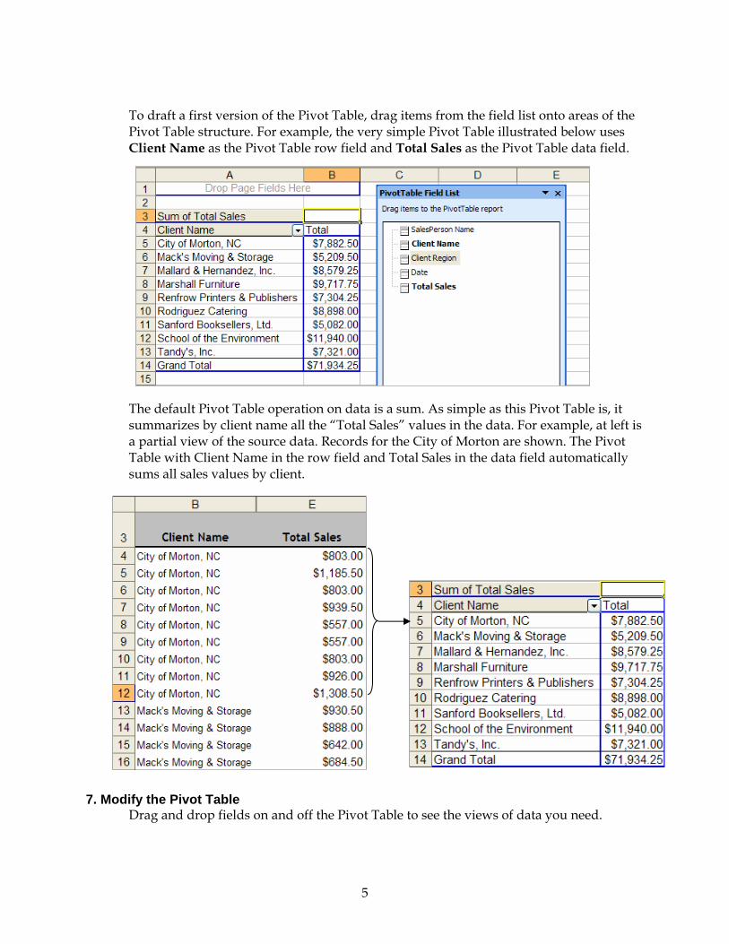
To draft a first version of the Pivot Table, drag items from the field list onto areas of the Pivot Table structure. For example, the very simple Pivot Table illustrated below uses Client Name as the Pivot Table row field and Total Sales as the Pivot Table data field.

The default Pivot Table operation on data is a sum. As simple as this Pivot Table is, it summarizes by client name all the “Total Sales” values in the data. For example, at left is a partial view of the source data. Records for the City of Morton are shown. The Pivot Table with Client Name in the row field and Total Sales in the data field automatically sums all sales values by client.

7. Modify the Pivot Table

Drag and drop fields on and off the Pivot Table to see the views of data you need.

5

More about the Pivot Table A Row Field

A row field in a Pivot Table is a variable that takes on different values. For example, a row field might be “Manufacturer” and its values might be “Schwinn”, “Cannondale”, and “Omega”. The values a variable takes on are sometimes referred to as “items”. In the example below, for each value of the variable “Manufacturer”, the Pivot Table displays a summary of the chosen data field in an adjoining column. The data field in this example is “Annual Sales” and the summary function is sum.

Sum of Annual SalesManufacturer TotalCannondale $823Omega $435Schwinn $500Grand Total $1,758

Notice that the Pivot Table uses the label “Sum of Annual Sales” to identify not only the data field (Annual Sales) but also the default summary operation (sum).

A Column Field

A Pivot Table column field works like a row field. A column field might be the variable “Year” with values ranging from 1995 to 1998. Data beneath each column in the Pivot Table is associated with the year at the head of the column.

Manufacturer Year Annual Sales Sum of Annual YearSchwinn 1995 $500 Manufacturer 1995 1996 1997 1998 Grand TotalCannondale 1995 $823 Cannondale 823 840 855 889 3407Omega 1995 $435 Omega 435 420 418 400 1673Schwinn 1996 $523 Schwinn 500 523 550 585 2158Cannondale 1996 $840 Grand Total 1758 1783 1823 1874 7238Omega 1996 $420Schwinn 1997 $550Cannondale 1997 $855Omega 1997 $418Schwinn 1998 $585Cannondale 1998 $889Omega 1998 $400

6

The basic effect of row and column fields in a Pivot Table is that each value or item that the field takes on defines a different row or column. So if a list has a row field with three items (Schwinn, Cannondale, Omega) and a column field that with four items (1995, 1996, 1997, 1998), the Pivot Table has three rows and four columns, and therefore twelve summary cells (exclusive of the cells that hold Grand Totals and labels).

A Data Field

The data field is the variable that the Pivot Table summarizes. For each combination of values in the row and column fields, the data field takes on a different value and this value appears in the Pivot Table’s cells. When you define a Pivot Table you must identify a data field or Excel displays an error. By contrast, however, you need not define either a row or a column field. If you build a Pivot Table with a data field only Excel won’t display an error message but the Pivot Table won’t provide a very meaningful result either. Without a row and/or column “control”, Excel returns a simple table since it has no way to summarize the data.

There are many summarizing calculations available in a Pivot Table. Most often the data to be summarized is numeric; the default summary for numeric data is a sum. For example, if your Pivot Table data field is Total Sales, the field dialog for Total Sales (below) shows that it can be summarized by sum, count, average, max, min, etc. If the data to be summarized is text data, not numeric, the default summary is count. For example “Employees” might be a data field and a Pivot Table might count of the number of employees by department.

Custom calculations can be applied to the data field, including running totals, percent of row, percent of column, and so on. If you need some calculation not provided within the Pivot Table, you can perform that calculation outside the context of the Pivot Table. Then you can include the calculated variable in your list when you start the Pivot Table

7

Wizard. The Pivot Table also has an option to create a calculated field and a calculated item. To explore these options, check Excel’s Pivot Table online help.

Data Plus Row Only or Data Plus Column Only If you specify a data field and a row field only, your Pivot Table will have one column that contains the values of the row field and another column to its right that contains the corresponding summary values for the data field. If you specify a data field and a column field only, your Pivot Table will have a top row that holds the values of the column field and a row beneath that holds the corresponding summary values of the data field.

Sum of Units SoldRegion Product TotalNortheast Brie 110

Gouda 128Northwest Brie 137

Gouda 151Southeast Brie 63

Gouda 72Southwest Brie 87Grand Total 748

Column-only Pivot Table

Sum of Annual SalesManufacturer TotalCannondale 3407Om 1ega 673Schwinn 2158Grand Total 7238

Sum of Annual Sales Year1995 1996 1997 1998 Grand Total

Total 1758 1783 1823 1874 7238

Row-only Pivot Table Drag and Drop

The Pivot Table gets its name because it’s easy to modify, or pivot, the positions of the Pivot Table fields. Imagine a point at the upper left-hand corner of the Pivot Table as the pivot point. You can drag and drop a row field up and to the right, making it a column field. And you can drag and drop a column field down and to the left, making it a row field. Although you can return to the Wizard’s layout view to make changes if you like it’s easier to do it on the fly without using the Wizard.

Inner Row or Inner Column Fields

If you have more than two variables in your list that you want to use as row or column fields you can define subsidiary or inner row or column fields.

In the example at left, “Product” is considered an inner row field while “Region” is the outer row field. The effect of an inner field is to add another level of detail to the Pivot Table. Within one category, or value (such as Northeast) of the outer field, there are two inner field values (Brie and Gouda). The data field is first summarized by the value of the outer row field. Within that first-level summary, the data field is further summarized by the corresponding values of the inner row field.

Inner and outer column fields work the same way as inner and outer row fields.

8

The Pivot Table Page Field The page field operates like the row and column fields but provides a third dimension to your data. It allows you to add another variable to your Pivot Table without necessarily viewing all its values at the same time.

In the example at left, the page field is “SalesPerson Name”. he default is to show data for (All) values.

Clicking the page field drop-down displays the page field values. Only two options are possible: (All) or the selection of one value from the drop-down.

Selecting a single page field value can greatly reduce the amount of data the Pivot Table displays.

A page field can be established in the initial draft of a Pivot Table or at any time afterward. A field designated as a page field can be removed or dragged to another area of the Pivot Table. A Pivot Table can have more than one page field.

9

Choose the Show Pages option at the bottom of the PivotTable drop-down menu on the Pivot Table toolbar to automatically generate a Pivot Table on a separate worksheet for each page field possibility.

Determining Pivot Table Layout A discrete variable generally has a relatively small number of unique values. Examples of discrete variables are department names, model names, or customer names. Discrete values are most suitable as row and column variables in a Pivot Table, although they can be used as data fields. For a discrete variable used as a data field, however, the Pivot Table will only be able to display a summary by count.

A continuous variable can take on a large range of values. Examples of continuous variables are profit margin, units sold, or dates. It’s generally not a good idea to use a continuous variable as a row or column field in a Pivot Table because a continuous variable can take on so many values that the Pivot Table would likely become impossibly large. For example, if you’re analyzing sales values for one year and you have 365 items of sales date data, you’re likely to run out of Excel worksheet display space if you make date a column field. Normally, you’d use a continuous variable as the data field in a Pivot Table in order to see the sum or average or other summary calculation of its values for different levels of discrete variables.

Partial view of a very wide Pivot Table where the continuous variable Date is used as a column field and the field holds individual days. “Grouping” is one method available to reduce the amount of data displayed.

10

Dates used as row or column headers, for example, are often grouped for this reason. Group a date field by right-clicking the field label, choosing Group and Show Detail from the initial context menu that displays and then choosing Group from the second context menu.

A special “Grouping” dialog displays. Excel suggests a grouping; you can choose a different grouping or more than one grouping. For example, one could choose to group date data both by Months and Quarters. In the illustration below, day dates as the row field have been grouped by both months and quarters. Excel figures out the quarters and makes that the outermost column field to group months. Days are grouped by month and form the innermost column field.

11

Formatting Data in the Pivot Table No matter what the format of the Pivot Table’s source data, the initial format of the data in a Pivot Table is “General”. After creating a Pivot Table you can use Excel’s normal formatting commands to format cells. To retain formatting when you refresh the data in a PivotTable or change the layout, do the following:

• Click a cell in the PivotTable, and on the Pivot Table toolbar choose the Pivot Table

button, then Table Options. In the “Format options” part of the dialog that displays, make sure the “Preserve formatting” check box is selected.

• Then, before you select the Pivot Table data you want to format, make sure that Pivot Table “Enable Selection” is activated (Choose the Pivot Table button on the toolbar, then Select, Enable Selection).

Without the steps above, if you make any change to your Pivot Table after you’ve applied formatting (even if the change is only to refresh the data), your formatting is lost.

A good method for formatting a numeric Pivot Table data field is to use the formatting options built into the Pivot Table itself. To do this: 1. Select any cell in the Pivot Table that represents its data field. 2. Click the Pivot Table Field button on the Pivot Table toolbar. The “Pivot Table Field”

dialog displays. 3. Click the Number button on this dialog to open the “Format Cells” dialog. 4. Choose one of the available formats, click OK to close the “Format Cells” dialog and

then OK again to close the “Pivot Table Field” dialog.

If you format your Pivot Table in this way, the formatting you select is retained even if you change the layout of the Pivot Table. This formatting is for numeric data only, not for text fields that might be used for row, column, or page fields.

12

To change the entire look of a Pivot Table, use the Pivot Table’s Format Report option (available from the Pivot Table toolbar drop-down menu). A new format you choose from the Pivot Table “AutoFormat” dialog remains with your Pivot Table even if you refresh the data, pivot the table, or add or remove a field.

The Pivot Table AutoFormat dialog displays ten table autoformats and ten report autoformats. A table-style autoformat

leaves the data arrangement alone and adds just formatting such as bolding, reverse video, etc. A report-style autoformat adds formatting but also rearranges the data so it’s column-oriented.

13

Refreshing Pivot Table Data A Pivot Table isn’t directly linked to its source data. Instead it’s linked to a hidden cache that’s build from the data source. If you create a Pivot Table from, for example, a worksheet list and then change the data in the list, the Pivot Table does not automatically update. To update the Pivot Table, click any cell within the Table and click the Refresh Data button (the red exclamation mark) on the Pivot Table toolbar. Then Excel gets the new data from your changed Excel list. As an alternative you can also right-click a cell in the Pivot Table and choose Refresh Data from the pop-up menu that appears.

Sorting Pivot Table Data

Excel usually displays a Pivot Table with field items in sorted order (ascending by rows for a row field and ascending by columns for a column field).

Ascending

Ascending

You may prefer to have your Pivot Table data sorted differently from the default. You can sort the Pivot Table either by labels or by values. There are two ways to sort Pivot Table data: “Externally” using Excel’s regular sorting feature, or “internally”, using the internal Pivot Table sort option. The internal sort you set remains even if you refresh the data (adding or deleting fields and values).

To Sort by Label using the “External” Method Choose the label to sort on. From Excel’s Data menu option choose Sort. Under “Sort by” choose Ascending or Descending. Under “Sort” choose Labels. Or, click an item and click the ascending or descending sort button on Excel’s Standard toolbar.

The “Sort” dialog at right sorts the Pivot Table below by “Client Region” in descending order.

14

To Sort by Label using the “Internal” Method If you choose to sort Pivot Table data using Excel’s “external” sort, the “Sort” dialog that displays reminds you that the Pivot Table also has its own sort. The advantage of the Pivot Table sort is that the sort is maintained even if the report data is updated or its layout changed. To sort is this way, double-click either the row field header or the column field header on which you want to sort. The Pivot Table opens the field dialog for that field. In that dialog, choose the Advanced button to open the Advanced Options field dialog, like the one illustrated below. Under “AutoSort Options” choose Ascending or Descending. For the “Using field” box, choose the field you’re sorting on. (A Manual sort is the default.)

To Sort by Pivot Table Data Values using the “External” Method If you don't care about retaining the sort sequence when you refresh the table, sort the data items manually using Excel’s regular sort. (If you’ve been using the Pivot Table AutoSort, reset the option to Manual, the default.) Then select the field you want to sort on and choose Data, Sort from Excel’s menus. In the “Sort by” box, enter the reference of a cell in the data area for the values you want to sort on. Or, click any cell in the Pivot Table data area and click either the ascending or descending sort button on Excel’s Standard toolbar.

Data sorted descending by Grand Total for rows using Excel’s Standard Toolbar sort button.

15

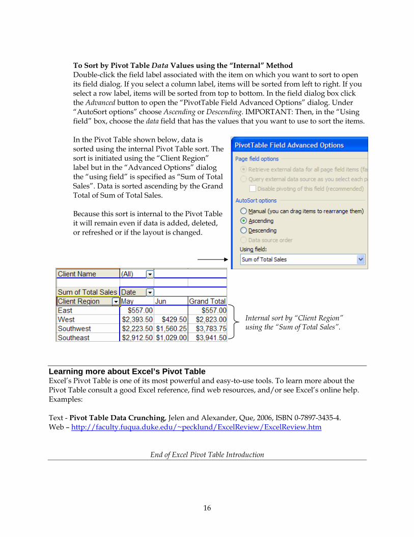
To Sort by Pivot Table Data Values using the “Internal” Method Double-click the field label associated with the item on which you want to sort to open its field dialog. If you select a column label, items will be sorted from left to right. If you select a row label, items will be sorted from top to bottom. In the field dialog box click the Advanced button to open the “PivotTable Field Advanced Options” dialog. Under “AutoSort options” choose Ascending or Descending. IMPORTANT: Then, in the “Using field” box, choose the data field that has the values that you want to use to sort the items.

In the Pivot Table shown below, data is sorted using the internal Pivot Table sort. The sort is initiated using the “Client Region” label but in the “Advanced Options” dialog the “using field” is specified as “Sum of Total Sales”. Data is sorted ascending by the Grand Total of Sum of Total Sales.

Because this sort is internal to the Pivot Table it will remain even if data is added, deleted, or refreshed or if the layout is changed.

Internal sort by “Client Region” using the “Sum of Total Sales”.

Learning more about Excel’s Pivot Table Excel’s Pivot Table is one of its most powerful and easy-to-use tools. To learn more about the Pivot Table consult a good Excel reference, find web resources, and/or see Excel’s online help. Examples: Text - Pivot Table Data Crunching, Jelen and Alexander, Que, 2006, ISBN 0-7897-3435-4. Web – http://faculty.fuqua.duke.edu/~pecklund/ExcelReview/ExcelReview.htm

End of Excel Pivot Table Introduction

16

17