An Introduction to Event History...

An Introduction to Event History Analysis

Oxford Spring SchoolJune 18-20, 2007

Day Two: Regression Models for Survival Data

Parametric Models

We’ll spend the morning introducing regression-like models for survival data, starting withfully parametric (distribution-based) models. These tend to be very widely used in socialsciences, although they receive almost no use outside of that (e.g., in biostatistics).

A General Framework (That Is, Some Math)

Parametric models are continuous-time models, in that they assume a continuous parametricdistribution for the probability of failure over time. A general parametric duration modeltakes as its starting point the hazard :

h(t) =f(t)

S(t)(1)

As we discussed yesterday, the density is the probability of the event (at T ) occurring withinsome differentiable time-span:

f(t) = lim∆t→0

Pr(t ≤ T < t + ∆t)

∆t. (2)

The survival function is equal to one minus the CDF of the density:

S(t) = Pr(T ≥ t)

= 1−∫ t

0

f(t) dt

= 1− F (t). (3)

This means that another way of thinking of the hazard in continuous time is as a conditionallimit:

h(t) = lim∆t→0

Pr(t ≤ T < t + ∆t|T ≥ t)

∆t(4)

i.e., the conditional probability of the event as ∆t gets arbitrarily small.

1

A General Parametric Likelihood

For a set of observations indexed by i, we can distinguish between those which are censoredand those which aren’t...

• Uncensored observations (Ci = 1) tell us both about the hazard of the event, and thesurvival of individuals prior to that event.

◦ That is, they tell us the exact time of failure.

◦ This means that, in terms of the likelihood, they contribute their density.

• Censored observations (Ci = 0) tell us only that that observation survived at least totime Ti.

◦ This means that they contribute information through their survival function.

We can thus combine these in a simple fashion, into a general parametric likelihood forsurvival models:

L =N∏

i=1

[f(Ti)]Ci [S(Ti)]

1−Ci (5)

with the corresponding log-likelihood:

lnL =N∑

i=1

{Ciln [f(Ti)] + (1− Ci)ln [S(Ti)]} (6)

which we can maximize using standard (e.g. Newton / Fisher scoring) methods. To includecovariates, we simply condition the terms of the likelihood on X and the associated parametervector β, e.g.

lnL =N∑

i=1

{Ciln [f(Ti|X, β)] + (1− Ci)ln [S(Ti|X, β)]} (7)

This general model can be thought of as encompassing all the various models we’ll discuss thismorning; the only differences among them are the distributions assumed for the probabilityof the event of interest.

2

The Exponential Model

The exponential is the simplest parametric duration model. There are (at least) two waysto motivate the exponential model. First, consider a model in which the hazard is constantover time:

h(t) = λ (8)

This model assumes that the hazard of an event is constant over time (i.e., “flat”), whichimplies that the conditional probability of the event is the same, no matter when the obser-vation is observed.

Put differently,

• Events occur according to a Poisson process (independent/“memoryless”).

• This also means that the accumulated/integrated hazard H(t) is simply the hazardtimes t, i.e.,

H(t) ≡∫ t

0

h(t) dt = λt (9)

Recalling that the survival function is equal to the exponentiated negative cumulative hazard:

S(t) = exp[−H(t)]

we can write the survival function for the exponential model as:

S(t) = exp(−λt) (10)

This, in turn, means that the density f(t) equals:

f(t) = h(t)S(t)

= λ exp(−λt) (11)

Given f(t) and S(t), we can plug these values into the log-likelihood equation (6) andestimate a value for λ via MLE.

3

Figure 1: Various Functions of an Exponential Model with λ = 0.02

Covariates

To introduce covariates, we have to consider that the hazard λ must always be positive. Thenatural solution is to allow the covariates to enter exponentially:

λi = exp(Xiβ). (12)

Note what this implies for the survival function: that

Si(t) = exp(−eXiβt). (13)

In other words, the survival function is “linked” to the covariates through a cumulativelog-log function. Similarly, the full log-likelihood for the exponential model becomes

lnL =N∑

i=1

{Ciln

[exp(Xiβ)exp(−eXiβt)

]+ (1− Ci)ln

[exp(−eXiβt)

]}=

N∑i=1

{Ci

[(Xiβ)(−eXiβt)

]+ (1− Ci)(−eXiβt)

}(14)

Estimation is accomplished via MLE of the likelihood in (14). We’ll get to interpretation ina bit...

4

Another Motivation: The Accelerated Failure Time Approach

Another motivation for parametric models is via a regression-type framework, involving amodel of the kind:

lnTi = Xiγ + εi (15)

That is, as an explicit regression-type model of (the log of) survival time. In this instance, weconsider the logged value mainly because survival time distributions tend to be right-skewed,and the exponential is a simple distribution with this characteristic.

This general format is known as the accelerated failure-time (AFT) form of duration models,and is most widely used in economics and engineering (though has also seen some use inbiostatistics in recent years). It corresponds to a model of

Ti = exp(Xiγ)× ui (16)

where εi = ln(ui). In this framework, we would normally posit that ui follows an exponentialdistribution, so that εi takes on what is known as an extreme value distribution, here withmean zero and variance equal to 1.0.

As in a standard regression model, we can rewrite model (16) as

εi = lnTi −Xiγ (17)

In standard fashion, then, the differences between the observed and predicted values (thatis, the residuals) follow an extreme-value distribution. We can then substitute these intothe likelihood given before, take derivatives w.r.t. the parameters of interest, set to zero andsolve to get our MLEs. Standard errors are obtained in the usual way, as the negative of the“information” matrix (the matrix of second derivatives of the log-likelihood with respect tothe parameters), and confidence intervals can be created by a “bounds” method.

A Note on the AFT Formulation

Parametric models are widely used in engineering, in studies of the reliability of components,etc. These studies often want to know, e.g., how long some piece of equipment will last beforeit “gives out.” But it’s often hard to do testing under typical circumstances – in particular,it can take too long.

In such situations, researchers expose equipment to more extreme conditions than will nor-mally be experienced (i.e., accelerate the failure process), and then do out-of-sample predic-tions. Under such circumstances, a fully parametric model is better than a semiparametricone which relies on intercomparability of subjects to assess covariate effects.

5

Which is better for social scientists? I’d argue that (most of the time) the Cox model is, butwe’ll talk more about that later today...

Interpretation

The exponential model can be interpreted in either AFT or hazard form. In either case,the coefficient estimates are identical, but the sign is reversed: variables which increase thehazard decrease the expected (log-) duration, and vice-versa.

Here is an example, with data on U.S. Supreme Court justice retirements (N = 107) and nocovariates (that is, we’re just estimating a model of the “mean” hazard/failure time):

Hazard rate form:

. streg , nohr dist(exp)

Exponential regression -- log relative-hazard form

No. of subjects = 107 Number of obs = 1765No. of failures = 51Time at risk = 1778

LR chi2(0) = -0.00Log likelihood = -100.83092 Prob > chi2 = .

------------------------------------------------------------------------------_t | Coef. Std. Err. z P>|z| [95% Conf. Interval]

-------------+----------------------------------------------------------------_cons | -3.551419 .140028 -25.36 0.000 -3.825869 -3.276969

------------------------------------------------------------------------------

6

AFT form:

. streg , time dist(exp)

Exponential regression -- accelerated failure-time form


LR chi2(0) = -0.00Log likelihood = -100.83092 Prob > chi2 = .


-------------+----------------------------------------------------------------_cons | 3.551419 .140028 25.36 0.000 3.276969 3.825869

------------------------------------------------------------------------------

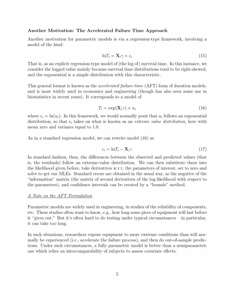
The AFT form has a very convenient interpretation: Since the “dependent variable” isln(T ), we can directly translate the estimated coefficient γ0 by noting that T = exp(γ0).That means that our estimated (mean) survival time is exp(3.5514) = 34.86.

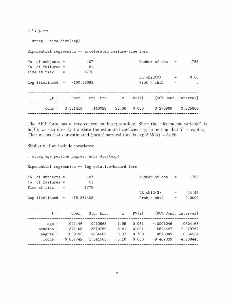
Similarly, if we include covariates:

. streg age pension pagree, nohr dist(exp)

Exponential regression -- log relative-hazard form


LR chi2(3) = 44.96Log likelihood = -78.351408 Prob > chi2 = 0.0000


-------------+----------------------------------------------------------------age | .041146 .0210568 1.95 0.051 -.0001246 .0824165

pension | 1.321105 .3870769 3.41 0.001 .5624487 2.079762pagree | .1069193 .2854665 0.37 0.708 -.4525849 .6664234_cons | -6.837742 1.341503 -5.10 0.000 -9.467039 -4.208445

------------------------------------------------------------------------------

7

. streg age pension pagree, time dist(exp)

Exponential regression -- accelerated failure-time form




-------------+----------------------------------------------------------------age | -.041146 .0210568 -1.95 0.051 -.0824165 .0001246

pension | -1.321105 .3870769 -3.41 0.001 -2.079762 -.5624487pagree | -.1069193 .2854665 -0.37 0.708 -.6664234 .4525849_cons | 6.837742 1.341503 5.10 0.000 4.208445 9.467039

------------------------------------------------------------------------------

Here,

• age is the justice’s age in years,

• pension is coded 1 if the justice is eligible for a pension, 0 if not, and

• pagree is coded 1 if the party of the sitting president is the same as the party of thepresident that appointed the justice, and 0 otherwise.

Once again, the coefficients in the AFT model have a simple interpretation: Every one unitchange in Xk corresponds to a change of 100× [1− exp(γk)] percent in the expected survivaltime. That means that, in this case:

• Every year older a justice is decreases their time on the Court by 100×[1−exp(−0.041)] =100× 0.0401 = 4.01 – that is, reduces it by approximately four percent.

• The availability of a pension decreases the predicted survival time by 100 × [1 −exp(−1.32)] = 100× (1− 0.267) = 73.3 – a whopping seventy three percent decrease.

8

Hazard Ratios

In the hazard rate model, the coefficients have a similarly easy interpretation. In consideringhazards, it is often useful to consider the hazard ratio: that is, the ratio of the hazard fortwo observations with different values of Xk:

HRk =h(t)|Xk = 1

h(t)|Xk = 0(18)

A hazard ratio of 1.0 corresponds to no difference in the hazard for the two observations;hazard ratios greater than one mean that the presence of the covariate increases the hazardof the event of interest, while a rate less than zero means that the covariate in questiondecreases that hazard.

In the context of the exponential model, note that, since we have defined h(t) = λ, a(conditional) constant, and λi = exp(Xiβ), then we can rewrite (12) as

hi(t) = exp(β0)exp(Xiβ)

This, in turn, means that the hazard ratio can be seen to be:

HRk =h(t)|Xk = 1

h(t)|Xk = 0

=exp(β0 + X1β1 + ... + βk(1) + ...)

exp(β0 + X1β1 + ... + βk(0) + ...)

=exp(βk)(1)

exp(βk)(0)

= exp(βk) (19)

In other words, the hazard ratio is just the exponentiated coefficient estimate from thehazard-rate form of the model. Thus, we would say that:

• A one-unit difference in the age of justices corresponds to a hazard ratio of exp(0.4115) =1.042. In words, the model suggests that the hazard of retirement for a given justiceis roughly 1.04 times that that of (or four percent greater than) a justice one year herjunior.

• Similarly, the hazard ratio of pension-eligible to non-pension-eligible justices is exp(1.32) =3.748; in words, the hazard for a retirement-eligible justice is nearly three times greaterthan one that is not so eligible.

More generally, the hazard ratio for two observations that differ by δ on the covariate Xk isjust

9

HRk =h(t)|Xk + δ

h(t)|Xk

= exp(δ βk)

Even more generally, the hazard ratio for two observations with covariate values Xi and Xj

is:

HR ij

=exp(Xiβ)

exp(Xjβ)(20)

Finally, note that equation (19) illustrates a key property of the exponential model: that itis a model of proportional hazards. This means that the hazards for any two observationswhich vary on a particular covariate are proportional to one another – or, alternatively, thatthe ratio of two such hazards is a constant with respect to time. This is a topic we’ll comeback to, as it has some potentially important implications.

The Weibull Model

The exponential model is nice enough, but the restriction that the hazard be constant overtime is often questioned in practice. In fact, we can imagine a number of processes where wemight expect hazard rates to be changing over time. If the (conditional) hazard is increasingor decreasing steadily over time, the exponential model will miss this fact.

The Weibull can be thought of as a hazard rate model in which the hazard is:

h(t) = λp(λt)p−1 (21)

Here, the parameter p is sometimes called a “shape parameter,” because it defines the shapeof the Weibull distribution.

• p = 1 corresponds to an exponential model (thus the Weibull “nests” the exponentialmodel),

• p > 1 means that the hazards are rising monotonically over time, and

• 0 < p < 1 means hazards are decreasing monotonically over time.

Recalling that the survival function can be expressed as the exponent of the negative inte-grated hazard, we can see that:

S(t) = exp

[−

∫ t

0

λp(λt)p−1 dt

]= exp(−λt)p (22)

10

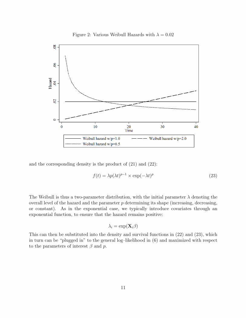
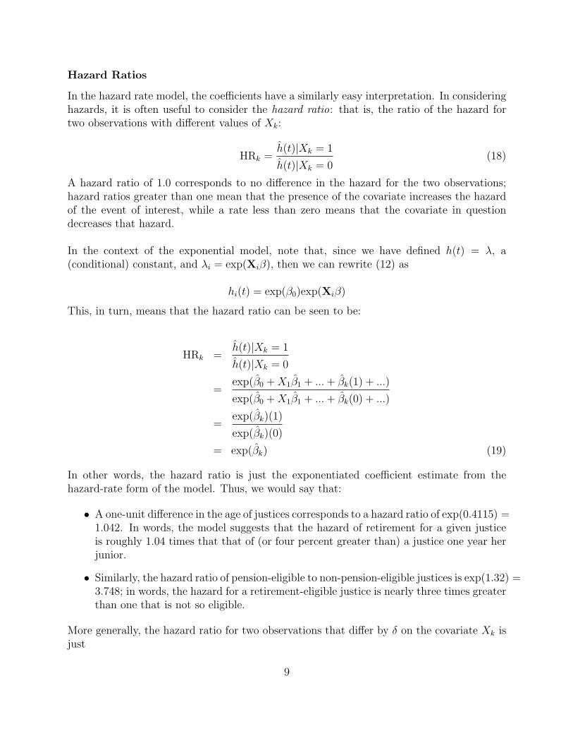
Figure 2: Various Weibull Hazards with λ = 0.02

and the corresponding density is the product of (21) and (22):

f(t) = λp(λt)p−1 × exp(−λt)p (23)

The Weibull is thus a two-parameter distribution, with the initial parameter λ denoting theoverall level of the hazard and the parameter p determining its shape (increasing, decreasing,or constant). As in the exponential case, we typically introduce covariates through anexponential function, to ensure that the hazard remains positive:

λi = exp(Xiβ)

This can then be substituted into the density and survival functions in (22) and (23), whichin turn can be “plugged in” to the general log–likelihood in (6) and maximized with respectto the parameters of interest β and p.

11

Figure 3: Various Weibull Survival Functions with λ = 0.02

The Weibull Model in an AFT formulation

As with the exponential model, the Weibull can also be considered a log-linear model oftime, but one where the errors are generalized. To do so, we replace equation (16) with amore general version:

Ti = exp(Xiγ)× σui (24)

In contrast to the AFT formulation of the exponential model, here the extreme-value distri-bution imposed upon the errors ui is not constrained to have variance equal to 1.0. Instead,the variance of the “errors” can take on any positive value. The result is a model where weestimate both the direct effects of the covariates on the (log of) survival time (γ) and thevariance of the “errors” (σ). Importantly, because of the nonlinearity of the model, thesetwo quantities are related; in particular, it is important to note that ∂Ti/∂X contains bothγ and σ. This reflects why some parameterizations of the Weibull model (particularly inengineering and economics, e.g., that of Greene) refer to “σ” rather than p.

12

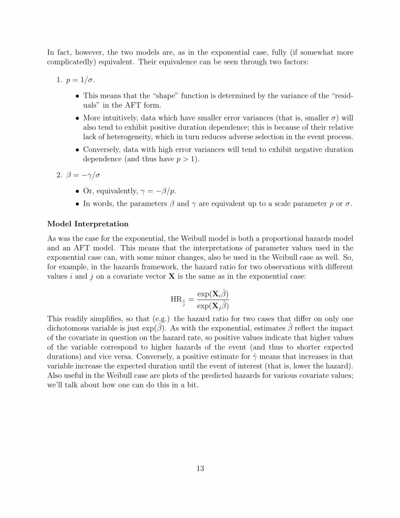
In fact, however, the two models are, as in the exponential case, fully (if somewhat morecomplicatedly) equivalent. Their equivalence can be seen through two factors:

1. p = 1/σ.

• This means that the “shape” function is determined by the variance of the “resid-uals” in the AFT form.

• More intuitively, data which have smaller error variances (that is, smaller σ) willalso tend to exhibit positive duration dependence; this is because of their relativelack of heterogeneity, which in turn reduces adverse selection in the event process.

• Conversely, data with high error variances will tend to exhibit negative durationdependence (and thus have p > 1).

2. β = −γ/σ

• Or, equivalently, γ = −β/p.

• In words, the parameters β and γ are equivalent up to a scale parameter p or σ.

Model Interpretation

As was the case for the exponential, the Weibull model is both a proportional hazards modeland an AFT model. This means that the interpretations of parameter values used in theexponential case can, with some minor changes, also be used in the Weibull case as well. So,for example, in the hazards framework, the hazard ratio for two observations with differentvalues i and j on a covariate vector X is the same as in the exponential case:

HR ij

=exp(Xiβ)

exp(Xjβ)

This readily simplifies, so that (e.g.) the hazard ratio for two cases that differ on only onedichotomous variable is just exp(β). As with the exponential, estimates β reflect the impactof the covariate in question on the hazard rate, so positive values indicate that higher valuesof the variable correspond to higher hazards of the event (and thus to shorter expecteddurations) and vice versa. Conversely, a positive estimate for γ means that increases in thatvariable increase the expected duration until the event of interest (that is, lower the hazard).Also useful in the Weibull case are plots of the predicted hazards for various covariate values;we’ll talk about how one can do this in a bit.

13

An Example

Consider again the models of Supreme Court retirements we discussed above:

. streg age pension pagree, nohr dist(weib)

Weibull regression -- log relative-hazard form




-------------+----------------------------------------------------------------age | .0405689 .0244068 1.66 0.096 -.0072675 .0884052

pension | 1.317683 .3935936 3.35 0.001 .5462542 2.089113pagree | .1084476 .2872933 0.38 0.706 -.4546368 .6715321_cons | -6.83356 1.344091 -5.08 0.000 -9.46793 -4.19919

-------------+----------------------------------------------------------------/ln_p | .0103713 .2216177 0.05 0.963 -.4239915 .444734

-------------+----------------------------------------------------------------p | 1.010425 .2239281 .6544294 1.560075

1/p | .9896823 .2193312 .6409947 1.528049------------------------------------------------------------------------------

. streg age pension pagree, time dist(weib)

Weibull regression -- accelerated failure-time form




-------------+----------------------------------------------------------------age | -.0401503 .0296687 -1.35 0.176 -.0982999 .0179993

pension | -1.304088 .5264274 -2.48 0.013 -2.335867 -.2723093pagree | -.1073287 .2826184 -0.38 0.704 -.6612506 .4465932_cons | 6.763054 2.0678 3.27 0.001 2.710241 10.81587

-------------+----------------------------------------------------------------/ln_p | .0103713 .2216177 0.05 0.963 -.4239915 .444734

-------------+----------------------------------------------------------------p | 1.010425 .2239281 .6544294 1.560075

1/p | .9896823 .2193312 .6409947 1.528049------------------------------------------------------------------------------

14

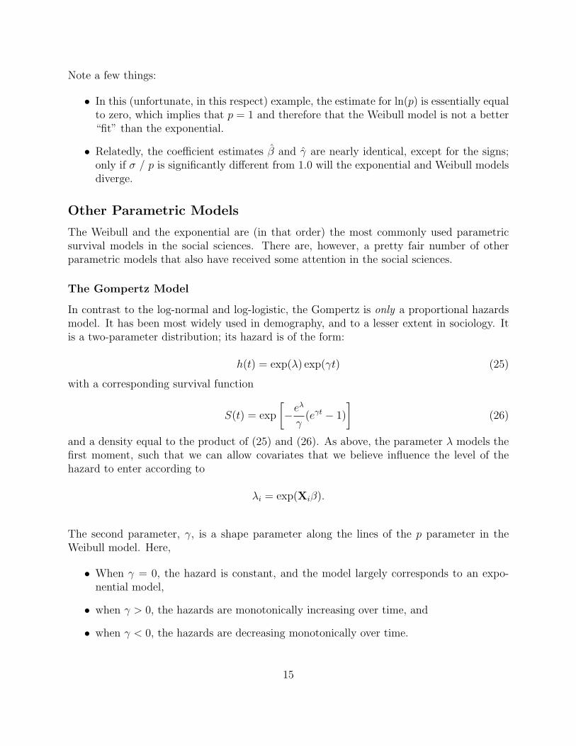
Note a few things:

• In this (unfortunate, in this respect) example, the estimate for ln(p) is essentially equalto zero, which implies that p = 1 and therefore that the Weibull model is not a better“fit” than the exponential.

• Relatedly, the coefficient estimates β and γ are nearly identical, except for the signs;only if σ / p is significantly different from 1.0 will the exponential and Weibull modelsdiverge.

Other Parametric Models

The Weibull and the exponential are (in that order) the most commonly used parametricsurvival models in the social sciences. There are, however, a pretty fair number of otherparametric models that also have received some attention in the social sciences.

The Gompertz Model

In contrast to the log-normal and log-logistic, the Gompertz is only a proportional hazardsmodel. It has been most widely used in demography, and to a lesser extent in sociology. Itis a two-parameter distribution; its hazard is of the form:

h(t) = exp(λ) exp(γt) (25)

with a corresponding survival function

S(t) = exp

[−eλ

γ(eγt − 1)

](26)

and a density equal to the product of (25) and (26). As above, the parameter λ models thefirst moment, such that we can allow covariates that we believe influence the level of thehazard to enter according to

λi = exp(Xiβ).

The second parameter, γ, is a shape parameter along the lines of the p parameter in theWeibull model. Here,

• When γ = 0, the hazard is constant, and the model largely corresponds to an expo-nential model,

• when γ > 0, the hazards are monotonically increasing over time, and

• when γ < 0, the hazards are decreasing monotonically over time.

15

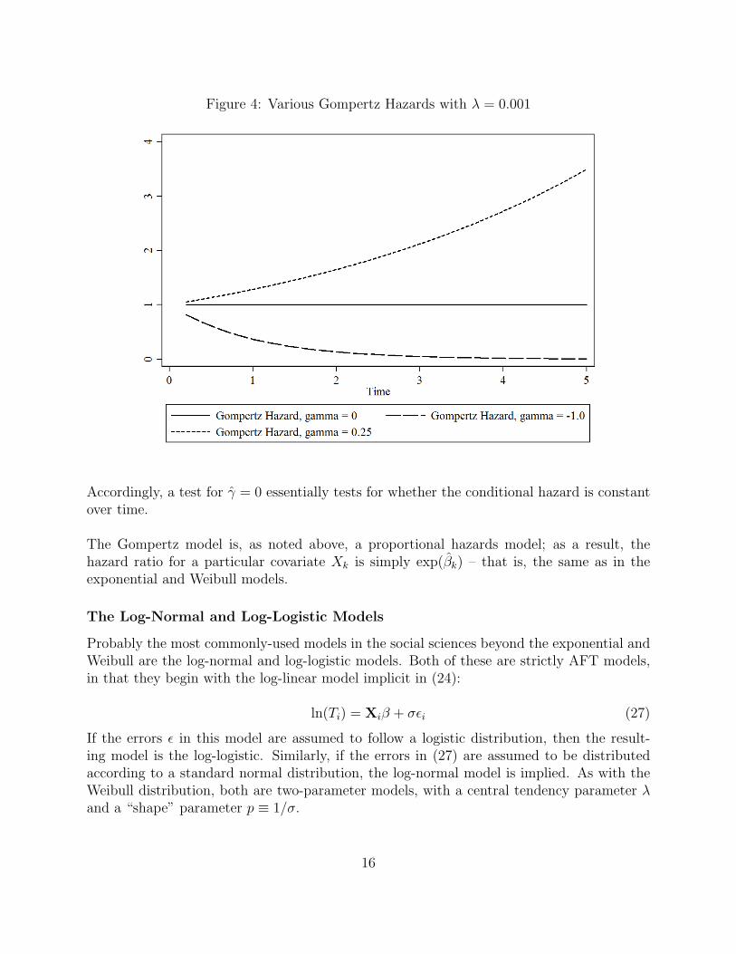
Figure 4: Various Gompertz Hazards with λ = 0.001

Accordingly, a test for γ = 0 essentially tests for whether the conditional hazard is constantover time.

The Gompertz model is, as noted above, a proportional hazards model; as a result, thehazard ratio for a particular covariate Xk is simply exp(βk) – that is, the same as in theexponential and Weibull models.

The Log-Normal and Log-Logistic Models

Probably the most commonly-used models in the social sciences beyond the exponential andWeibull are the log-normal and log-logistic models. Both of these are strictly AFT models,in that they begin with the log-linear model implicit in (24):

ln(Ti) = Xiβ + σεi (27)

If the errors ε in this model are assumed to follow a logistic distribution, then the result-ing model is the log-logistic. Similarly, if the errors in (27) are assumed to be distributedaccording to a standard normal distribution, the log-normal model is implied. As with theWeibull distribution, both are two-parameter models, with a central tendency parameter λand a “shape” parameter p ≡ 1/σ.

16

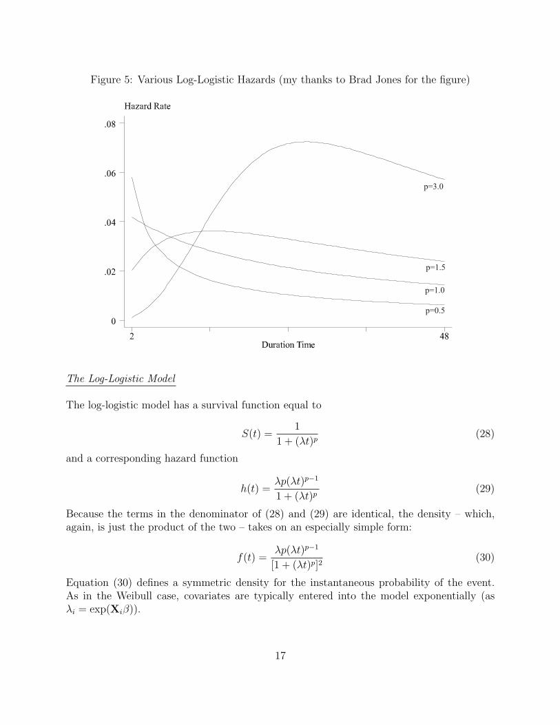
Figure 5: Various Log-Logistic Hazards (my thanks to Brad Jones for the figure)

The Log-Logistic and Log-Normal Models

log(T ) = !!jx + "#. (11)

Log-Logistic:

h(t) =$p($t)p"1

1 + ($t)p(12)

Figure 3: This figure graphs some typically shaped hazard rates for the log-logistic model.

S(t) =1

1 + ($t)p, (13)

f(t) =$p($t)p"1

(1 + ($t)p)2, (14)

4

The Log-Logistic Model

The log-logistic model has a survival function equal to

S(t) =1

1 + (λt)p(28)

and a corresponding hazard function

h(t) =λp(λt)p−1

1 + (λt)p(29)

Because the terms in the denominator of (28) and (29) are identical, the density – which,again, is just the product of the two – takes on an especially simple form:

f(t) =λp(λt)p−1

[1 + (λt)p]2(30)

Equation (30) defines a symmetric density for the instantaneous probability of the event.As in the Weibull case, covariates are typically entered into the model exponentially (asλi = exp(Xiβ)).

17

Important : Note that many software packages – including Stata – parameterize p as γ = 1p.

Bear this in mind as you consider your actual results.

The Log-Normal Model

The log–normal model is very similar to the log-logistic, in that the density of the “errors” εare assumed to have a bell-shaped symmetrical (here, standard normal) distribution. If wethink of the “errors” as being normally distributed (that is, as φ(·)), then the cumulativeerrors are cumulative normal. Because of that, we can write the survival function for thelog-normal as:

S(t) = 1− Φ

[lnT − ln(λ)

σ

](31)

Log-Logistic / Log-Normal Commonalities

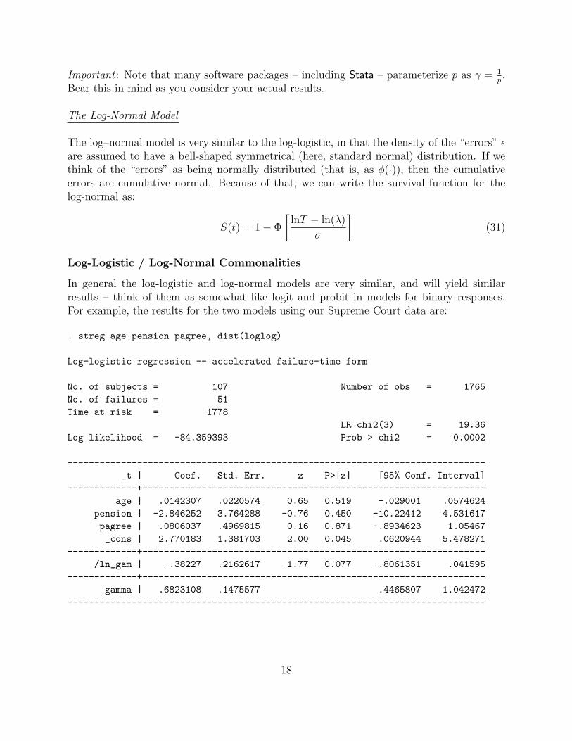
In general the log-logistic and log-normal models are very similar, and will yield similarresults – think of them as somewhat like logit and probit in models for binary responses.For example, the results for the two models using our Supreme Court data are:

. streg age pension pagree, dist(loglog)

Log-logistic regression -- accelerated failure-time form




-------------+----------------------------------------------------------------age | .0142307 .0220574 0.65 0.519 -.029001 .0574624

pension | -2.846252 3.764288 -0.76 0.450 -10.22412 4.531617pagree | .0806037 .4969815 0.16 0.871 -.8934623 1.05467_cons | 2.770183 1.381703 2.00 0.045 .0620944 5.478271

-------------+----------------------------------------------------------------/ln_gam | -.38227 .2162617 -1.77 0.077 -.8061351 .041595

-------------+----------------------------------------------------------------gamma | .6823108 .1475577 .4465807 1.042472

------------------------------------------------------------------------------

18

. streg age pension pagree, dist(lognorm)

Log-normal regression -- accelerated failure-time form




-------------+----------------------------------------------------------------age | -.0124893 .029725 -0.42 0.674 -.0707492 .0457705

pension | -3.598691 1.642479 -2.19 0.028 -6.817891 -.379491pagree | .0354144 .4266008 0.08 0.934 -.8007078 .8715367_cons | 4.632599 1.873923 2.47 0.013 .9597768 8.305422

-------------+----------------------------------------------------------------/ln_sig | .3819538 .2020201 1.89 0.059 -.0139983 .777906

-------------+----------------------------------------------------------------sigma | 1.465144 .2959887 .9860992 2.176909

------------------------------------------------------------------------------

Also, a key trait of both the log-normal and log-logistic models is that they allow for thepossibility of non-monotonic hazards. In particular, the log–logistic model with p > 1, andthe log-normal for most values of p, both have hazards which first rise, then fall over time.

The Generalized Gamma Model

The generalized gamma is, as the model suggests, a general model that “nests” a number ofothers. The survival function is:

S(t) = 1− Γ

{κ, κ exp

[lnTi−λ

σ

κ1/2

]}(32)

Here, Γ(·) is the indefinite gamma integral. The formulae for the hazard and the densityare complicated, and largely beside the point. The more important thing is that the modelnests the lognormal, Weibull and exponential models:

• The model is log-normal as κ →∞.

• the model is a Weibull when κ = 1,

• the model is exponential when κ = σ = 1.

19

This model is thus nice and general, but can be slooooow and difficult to get to converge. Forexample, using our Supreme Court retirements example data, the model wouldn’t convergeat all:

. streg age pension pagree, dist(gamma)

Fitting constant-only model:

Iteration 0: log likelihood = -179.4614 (not concave)Iteration 1: log likelihood = -101.39199Iteration 2: log likelihood = -92.677695Iteration 3: log likelihood = -90.945899Iteration 4: log likelihood = -90.415731Iteration 5: log likelihood = -90.114788Iteration 6: log likelihood = -89.913238Iteration 7: log likelihood = -89.84974Iteration 8: log likelihood = -89.820951Iteration 9: log likelihood = -89.814303Iteration 10: log likelihood = -89.809908Iteration 11: log likelihood = -89.809583Iteration 12: log likelihood = -89.809157discontinuous region encounteredcannot compute an improvementr(430);

Estimation and Interpretation (With a Running Example)

For the rest of the morning, we’ll focus on the mechanics of the estimation, selection, inter-pretation, and presentation of parametric models for survival data. To do this, we’ll use arunning example, based on the analysis and data in:

Brooks, Sarah M. 2005. “Interdependent and Domestic Foundations of Policy Change.” In-ternational Studies Quarterly 49(2):273-294.

Brooks’ major focus is the causes of pension privatization. In particular, Brooks is interestedin the extent to which nations’ decisions to privatize their pension plans are interdependent –that is, whether or not they reflect similar decisions by other nations. Her primary responsevariable is the onset of pension privatization in 59 countries in the OECD, Latin America,Eastern Europe, and Central Asia between 1980 and 1999.

Given this interest in diffusion, Brooks’ key covariate of interest is peer privatization – oper-ationalized as the proportion (really the percentage) of countries in each of the three “peergroups” (OECD, Latin America, and Eastern Europe and Central Asia) that have priva-tized. Brooks’ main expectations are that the influence of peer privatization will vary across

20

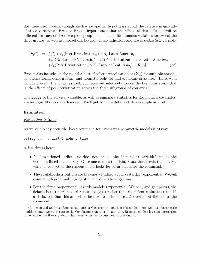
the three peer groups, though she has no specific hypotheses about the relative magnitudeof those variations. Because Brooks hypothesizes that the effects of this diffusion will bedifferent for each of the three peer groups, she include dichotomous variables for two of thethree groups, as well as interactions between those indicators and the privatization variable:

hi(t) = f [β0 + β1(Peer Privatizationit) + β2(Latin Americai)

+β3(E. Europe/Cent. Asiai) + β4(Peer Privatizationit × Latin Americai)

+β5(Peer Privatizationit × E. Europe/Cent. Asiai) + Xitγ] (33)

Brooks also includes in the model a host of other control variables (Xit) for such phenomenaas international, demographic, and domestic political and economic pressures.1 Here, we’llinclude these in the model as well, but focus out interpretation on the key covariates – thatis, the effects of peer privatization across the three subgroups of countries.

The stdes of the survival variable, as well as summary statistics for the model’s covariates,are on page 10 of today’s handout. We’ll get to more details of this example in a bit.

Estimation

Estimation in Stata

As we’ve already seen, the basic command for estimating parametric models is streg:

.streg ... , dist() nohr / time ...

A few things here:

• As I mentioned earlier, one does not include the “dependent variable” among thevariables listed after streg. Once one stsets the data, Stata then treats the survivalvariable you set as the response, and looks for covariates after the command.

• The available distributions are the ones we talked about yesterday: exponential, Weibull,gompertz, log-normal, log-logistic, and generalized gamma.

• For the three proportional hazards models (exponential, Weibull, and gompertz), thedefault is to report hazard ratios (exp(β)s) rather than coefficient estimates (βs). If,as I do, you find this annoying, be sure to include the nohr option at the end of thecommand.

1In her actual analysis, Brooks estimates a Cox proportional hazards model; here, we’ll use parametricmodels, though we can return to the Cox formulation later. In addition, Brooks include a log-time interactionin her model; we’ll worry about that later, when we discuss nonproportionality.

21

• Likewise, for those models that have both PH and AFT implementations, the default isthe PH form. If you prefer the accelerated failure-time approach, the option to includeis time.

Most of these models converge well and generally are well-behaved, with the notable excep-tion of the generalized gamma model. The results of estimating each of these models forBrooks’ data are on pages 2-4 of the handout.

Estimation in R

In general, R is not as good for parametric models as is Stata (this is in contrast to the Coxmodel). After loading the survival package, the basic command is survreg:

Results<-survreg(Surv(duration, censor)~X1+X2+X3, dist="exponential")

Note a couple things:

1. Available distributions are exponential, Weibull, normal, logistic, log-normal, and log-logistic.

2. To the best of my knowledge, R will not estimate parametric models with time-varyingdata/covariates. This is a big drawback, and really means that you’re much better offusing Stata for those models.

Model Selection

Theory

If possible, use it. It is generally better than all of the alternatives. Points to consider:

• Can you, from first principles, derive a data-generating process for the phenomenon un-der study that leads more-or-less directly to a particular parametric distribution?(If you can, you’re very lucky, at least in the social scoences...).

• Are there theoretical expectations about how events ought to arise? Conditional onX, is there reason to expect that events might not be independent of one another(and so that the exponential might not be a good representation of the edata)?

• Is there some reason to expect the (conditional) shape of the hazard to take on aparticular form?

22

Statistical Tests

If you have no theory, or if the theory is vague or otherwise indeterminate, then one can useformal statistical tests to choose among models There are two main sorts of these that wemight be interested in here.

1. LR Tests

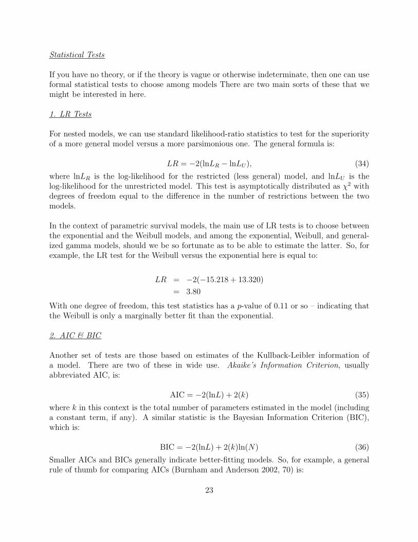
For nested models, we can use standard likelihood-ratio statistics to test for the superiorityof a more general model versus a more parsimonious one. The general formula is:

LR = −2(lnLR − lnLU), (34)

where lnLR is the log-likelihood for the restricted (less general) model, and lnLU is thelog-likelihood for the unrestricted model. This test is asymptotically distributed as χ2 withdegrees of freedom equal to the difference in the number of restrictions between the twomodels.

In the context of parametric survival models, the main use of LR tests is to choose betweenthe exponential and the Weibull models, and among the exponential, Weibull, and general-ized gamma models, should we be so fortunate as to be able to estimate the latter. So, forexample, the LR test for the Weibull versus the exponential here is equal to:

LR = −2(−15.218 + 13.320)

= 3.80

With one degree of freedom, this test statistics has a p-value of 0.11 or so – indicating thatthe Weibull is only a marginally better fit than the exponential.

2. AIC & BIC

Another set of tests are those based on estimates of the Kullback-Leibler information ofa model. There are two of these in wide use. Akaike’s Information Criterion, usuallyabbreviated AIC, is:

AIC = −2(lnL) + 2(k) (35)

where k in this context is the total number of parameters estimated in the model (includinga constant term, if any). A similar statistic is the Bayesian Information Criterion (BIC),which is:

BIC = −2(lnL) + 2(k)ln(N) (36)

Smaller AICs and BICs generally indicate better-fitting models. So, for example, a generalrule of thumb for comparing AICs (Burnham and Anderson 2002, 70) is:

23

AICModel j - AICMinimum-AIC Model Level of Empirical Support for Model j0-2 Substantial4-7 Considerably Less

> 10 Essentially None

The AICs and BICs for each of the five models estimated (generated using Stata’s estat ic

command after estimation) are reported here:

Table 1: lnL, AIC, and BIC for Five Parametric Models

Model lnL AIC BICExponential -15.218 64.436 144.14Weibull -13.320 62.640 147.03Gompertz -14.059 64.118 148.51Log-Normal -15.224 66.447 150.84Log-Logistic -14.310 64.620 149.01

By a pure AIC-minimization criterion, the Weibull model wins out, with the Gompertz com-ing in second, edging out the exponential. If we pay attention to the BIC – which penalizesadditional parameters more than the AIC does – then the exponential is our model. Ofcourse, none of these can tell you whether your model is any good in absolute terms; at best,they can be useful for choosing among relatively similar models.

Fitted Values

A more impressionistic approach is to examine the fitted values of each model. These can beany number of things, though the most natural quantity to examine is the predicted durationor log-duration, since that is the easiest to compare to the actual values. Stata (and mostother programs) makes generating such values relatively easy:

. predict lnThat_E, median lntime

When we plot the predicted log-median durations for our five models against their (alsologged) actual values for those observations that privatized, we get:

24

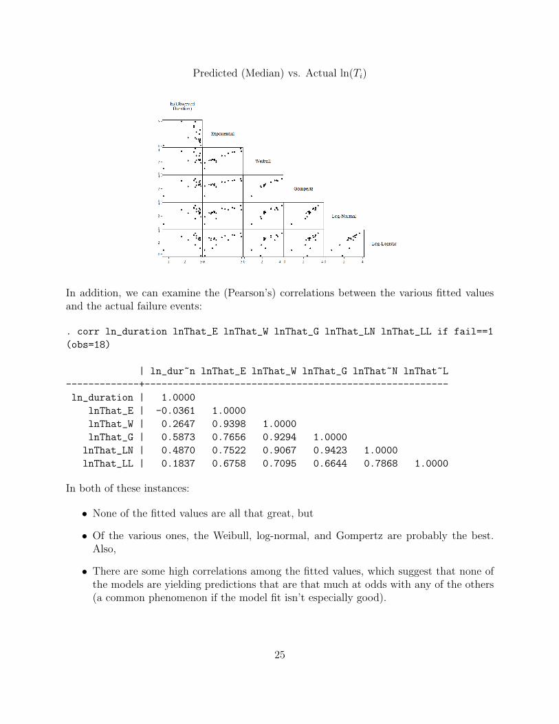
Predicted (Median) vs. Actual ln(Ti)

In addition, we can examine the (Pearson’s) correlations between the various fitted valuesand the actual failure events:

. corr ln_duration lnThat_E lnThat_W lnThat_G lnThat_LN lnThat_LL if fail==1

(obs=18)

| ln_dur~n lnThat_E lnThat_W lnThat_G lnThat~N lnThat~L

-------------+------------------------------------------------------

ln_duration | 1.0000

lnThat_E | -0.0361 1.0000

lnThat_W | 0.2647 0.9398 1.0000

lnThat_G | 0.5873 0.7656 0.9294 1.0000

lnThat_LN | 0.4870 0.7522 0.9067 0.9423 1.0000

lnThat_LL | 0.1837 0.6758 0.7095 0.6644 0.7868 1.0000

In both of these instances:

• None of the fitted values are all that great, but

• Of the various ones, the Weibull, log-normal, and Gompertz are probably the best.Also,

• There are some high correlations among the fitted values, which suggest that none ofthe models are yielding predictions that are that much at odds with any of the others(a common phenomenon if the model fit isn’t especially good).

25

Interpretation

Stata has a huge number of useful post-estimation commands. I won’t go into all of themhere – we’ll skip a discussion of test, testnl, mfx, etc. – but discuss several other usefulcomplements to streg.

Hazard Ratios

As we discussed earlier, for models that have a hazard-rate form, hazard ratios are a nice,intuitive way of talking about the marginal effects of covariates.

• Just exp(βk).

• Stata reports them automatically if you want it to (cf. p. 6 of the handout).

• Discussing them:

◦ HRs reflect the relative/proportional change in h(t) associated with a unit changein Xk. In other words, they are invariant to the values of the other covariates, orof the hazard itself.

◦ Similarly, remember that 100 × (HR - 1) is the same thing as the percentagechange in the hazard associated with a one-unit change in the covariate in ques-tion.

◦ Also remember that the hazard ratios reported by Stata are for one-unit changesin Xk. That means that if a one-unit change in Xk is either very large or verysmall, the hazard ratios will be the opposite.

◦ That, in turn, suggests that if you’re going to use hazard ratios for reportingand discussing your results, it’s a good idea to rescale your covariates so that aone-unit change is meaningful.

So, let’s discuss some of the hazard ratios for the “full” Weibull model:

• worldbank (X = 0.07, σ = 0.48, HR = 0.601)

◦ A measure of “hard power,” in the form of the level of World Bank loans or creditsto the country.

◦ The hazard ratio of 0.601 means that, among two otherwise-identical observationsthat differ by one unit on worldbank, the one with the higher level of the variablewill have a hazard that is 60.1 percent the size of the former.

◦ Likewise, each unit increase in worldbank decreases the hazard of privatizationby 100 × (0.601 - 1) ≈ 40 percent.

◦ The confidence intervals, however, are very wide, and encompass 1.0; this meansthat we cannot say this result is not due to chance.

26

• age65 (X = 9.73, σ = 4.68, HR = 1.35)

◦ Measures the percentage of the population that is over the age of 65.

◦ The hazard ratio of 1.35 means that, among two otherwise-identical observationsthat differ by one unit on age65, the one with the higher level of the variable willhave a hazard that is 1.35 times as large as the former.

◦ Likewise, each unit increase in age65 increases the hazard of privatization by 100× (1.35 - 1) ≈ 35 percent.

◦ The confidence intervals suggest that this variable is “statistically significant” /“bounded away from zero” in its effect. The 95 percent credible range for thehazard ratio ranges from 1.04 to 1.76.

• deficit (X = −3.68, σ = 4.27, HR = 1.24)

◦ Brooks calls it Budget Balance; it’s an indicator of the overall level of surplus ordeficit in that country in that year, as a percentage of GDP.

◦ Similar to age65, the hazard ratio of 1.24 means that, among two otherwise-identical observations that differ by one unit on deficit, the one with the higherlevel of the variable will have a hazard that is 1.24 times as large as the former.

◦ If we want to know (say) the impact of a five-percent swing in the budget deficit,we can calculate that as exp(0.214 × 5) ≈ 2.92. This means that a five-percentincrease in the budget deficit (as a percent of GDP) nearly triples the hazard ofpension privatization.

◦ Once again, the 95-percent confidence interval (barely) excludes 1.0, meaningthat the estimated effect is “statistically significant” at conventional (p = .05,two-tailed) levels.

We’ll discuss the hazard ratios for the main (interactive) variables of interest in a bit...

Obtaining Linear (and Nonlinear) Combinations of Parameters

Stata offers some nice commands for obtaining linear and nonlinear combinations of estimatedparameters, as well as the standard errors, p-values, and confidence intervals associated withthose combinations. These are particularly valuable when – as we have here – there areinteraction effects in our models.

27

Combinations of βs: lincom

We can obtain estimates of linear combinations of parameters (as in, our estimated coeffi-cients) using lincom. Suppose we want to know the “quasi-coefficient” of Peer Privatizationfor Latin American countries. In terms of our model in (33), this is equal to:

βPeer Privatization|Latin America = β1 + β4

and the equivalent coefficient estimate for the Eastern European and Central Asian countriesis:

βPeer Privatization|E. Europe / Cent. Asia = β1 + β5.

After estimating our model, lincom has Stata calculate this quantity for us, along with itsassociated uncertainty quantities:

. lincom(peerprivat+LatAmxPeer)

( 1) [_t]peerprivat + [_t]LatAmxPeer = 0

------------------------------------------------------------------------------

_t | Coef. Std. Err. z P>|z| [95% Conf. Interval]

-------------+----------------------------------------------------------------

(1) | .1055036 .0457227 2.31 0.021 .0158887 .1951185

------------------------------------------------------------------------------

This tells us that the effect of Peer Privatization on the hazard of privatization in LatinAmerican countries is positive and “statistically significant” at conventional levels. We cando the same thing for the Eastern European and Central Asian countries:

. lincom(peerprivat+EECAxPeer)

( 1) [_t]peerprivat + [_t]EECAxPeer = 0

------------------------------------------------------------------------------


-------------+----------------------------------------------------------------

(1) | .0531117 .0448715 1.18 0.237 -.0348348 .1410581

------------------------------------------------------------------------------

...where we see that the effect of that variable is not significantly different from zero in thosecountries.

28

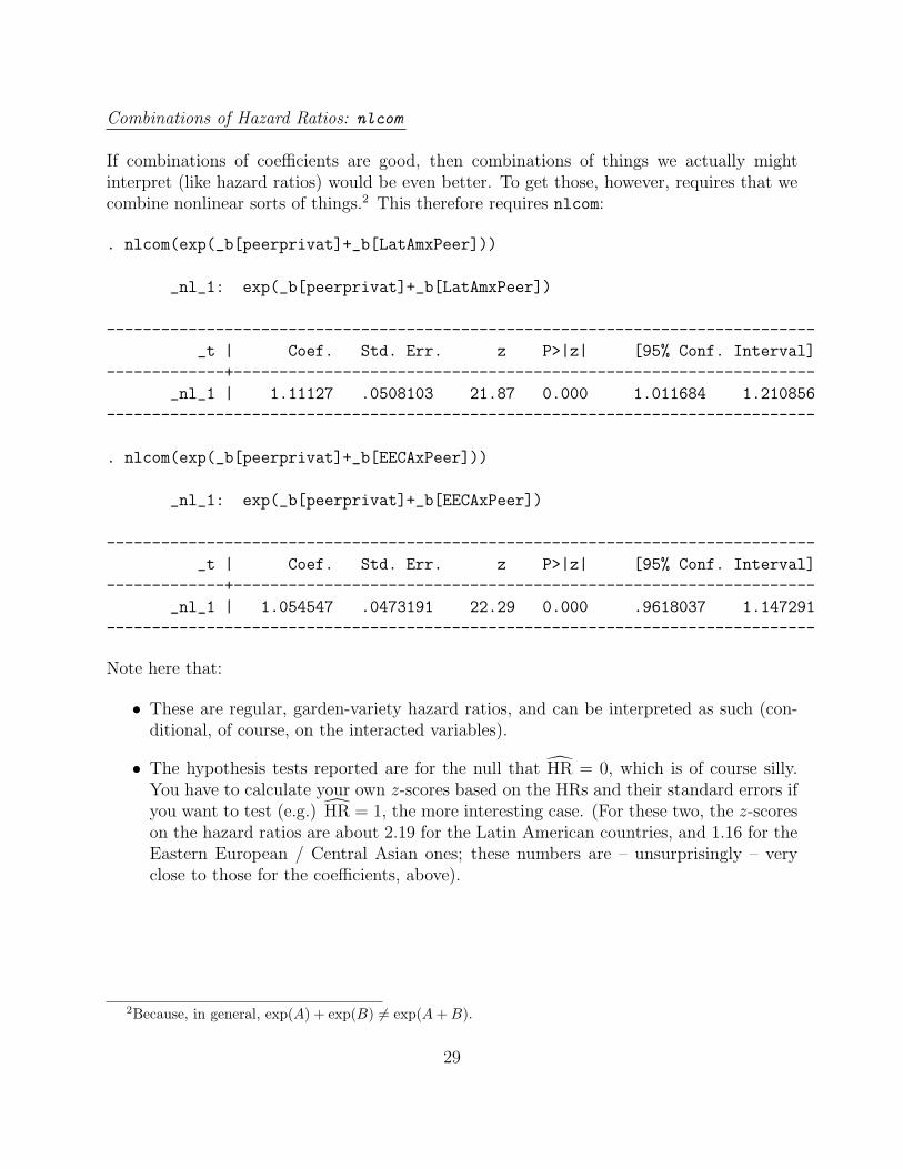
Combinations of Hazard Ratios: nlcom

If combinations of coefficients are good, then combinations of things we actually mightinterpret (like hazard ratios) would be even better. To get those, however, requires that wecombine nonlinear sorts of things.2 This therefore requires nlcom:

. nlcom(exp(_b[peerprivat]+_b[LatAmxPeer]))

_nl_1: exp(_b[peerprivat]+_b[LatAmxPeer])

------------------------------------------------------------------------------


-------------+----------------------------------------------------------------

_nl_1 | 1.11127 .0508103 21.87 0.000 1.011684 1.210856

------------------------------------------------------------------------------

. nlcom(exp(_b[peerprivat]+_b[EECAxPeer]))

_nl_1: exp(_b[peerprivat]+_b[EECAxPeer])

------------------------------------------------------------------------------


-------------+----------------------------------------------------------------

_nl_1 | 1.054547 .0473191 22.29 0.000 .9618037 1.147291

------------------------------------------------------------------------------

Note here that:

• These are regular, garden-variety hazard ratios, and can be interpreted as such (con-ditional, of course, on the interacted variables).

• The hypothesis tests reported are for the null that HR = 0, which is of course silly.You have to calculate your own z-scores based on the HRs and their standard errors ifyou want to test (e.g.) HR = 1, the more interesting case. (For these two, the z-scoreson the hazard ratios are about 2.19 for the Latin American countries, and 1.16 for theEastern European / Central Asian ones; these numbers are – unsurprisingly – veryclose to those for the coefficients, above).

2Because, in general, exp(A) + exp(B) 6= exp(A + B).

29

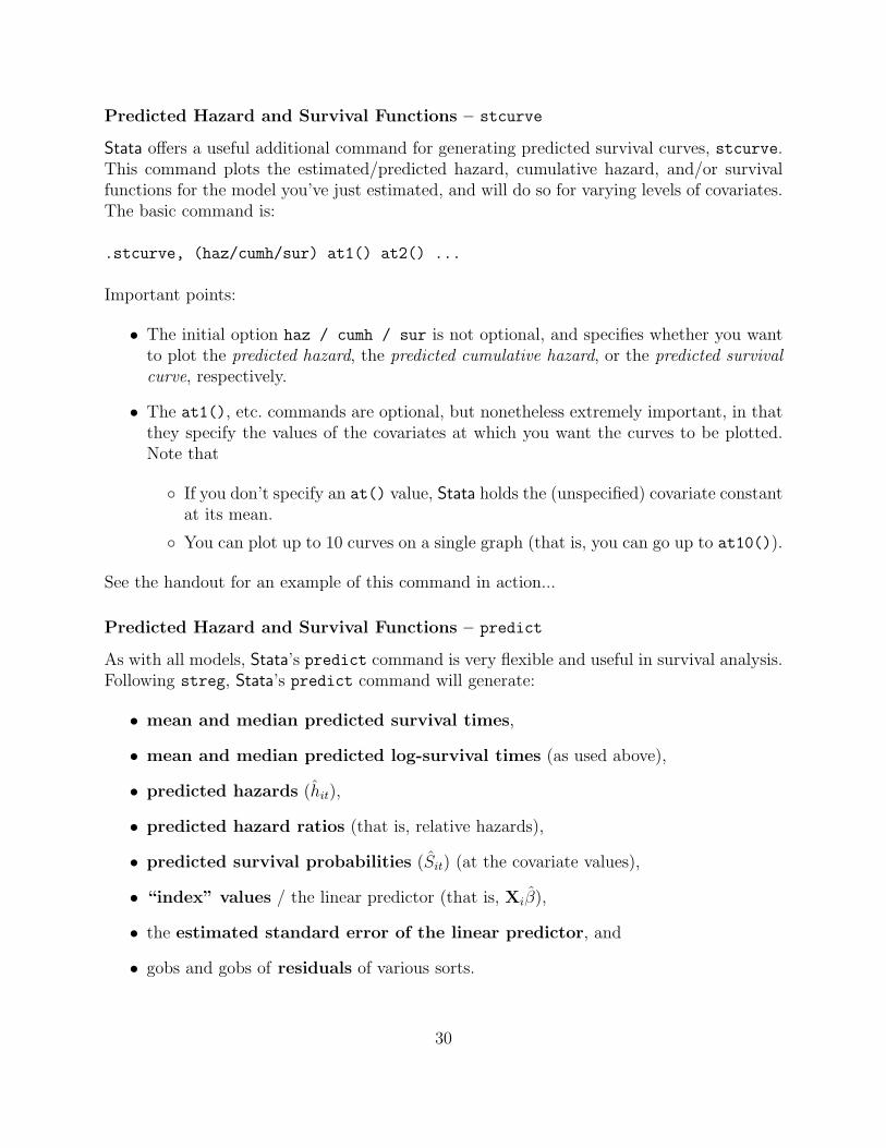
Predicted Hazard and Survival Functions – stcurve

Stata offers a useful additional command for generating predicted survival curves, stcurve.This command plots the estimated/predicted hazard, cumulative hazard, and/or survivalfunctions for the model you’ve just estimated, and will do so for varying levels of covariates.The basic command is:

.stcurve, (haz/cumh/sur) at1() at2() ...

Important points:

• The initial option haz / cumh / sur is not optional, and specifies whether you wantto plot the predicted hazard, the predicted cumulative hazard, or the predicted survivalcurve, respectively.

• The at1(), etc. commands are optional, but nonetheless extremely important, in thatthey specify the values of the covariates at which you want the curves to be plotted.Note that

◦ If you don’t specify an at() value, Stata holds the (unspecified) covariate constantat its mean.

◦ You can plot up to 10 curves on a single graph (that is, you can go up to at10()).

See the handout for an example of this command in action...

Predicted Hazard and Survival Functions – predict

As with all models, Stata’s predict command is very flexible and useful in survival analysis.Following streg, Stata’s predict command will generate:

• mean and median predicted survival times,

• mean and median predicted log-survival times (as used above),

• predicted hazards (hit),

• predicted hazard ratios (that is, relative hazards),

• predicted survival probabilities (Sit) (at the covariate values),

• “index” values / the linear predictor (that is, Xiβ),

• the estimated standard error of the linear predictor, and

• gobs and gobs of residuals of various sorts.

30

As in all cases, you can use predict either in- or out-of-sample. That means you can generate“simulated” data with particular characteristics of interest, and then predict to them. Thisis, at the moment, the only way I’m aware of to get things like confidence intervals aroundpredictions; moreover, it tends to be a bit clunky, since in order to predict from an -st-

model, the data must be -st- as well. There are some ways to “fool” Stata into doing this,but they’re all a bit artificial.

Finally: A Couple Things That Don’t Work

1. Clarify (with any of the -st- commands).

2. Zelig will work, but only with non-time-varying data (since that’s all that R willestimate as well).

If any of you nerdy folks care to write the code that will make either of these things moreuseful, the world would thank you (and I might even buy you a beer).

31

Cox’s Semiparametric Model

The model introduced by Cox (1972) is arguably the single most important tool for survivalanalysis available today. It is by far the most widely-used model in biostatistics, epidemiol-ogy, and other “hard-science” fields, and is increasingly becoming so in the social sciences.The reasons for this popularity will become apparent in a minute.

This afternoon we’ll introduce the Cox model, which is also sometimes (slightly inaccurately)known as “the proportional hazards model.” We’ll talk about estimation, and interpretationof that model, and we’ll walk through an example in the Stata and R packages.

Cox’s (1972) Semiparametric Hazard Model

Consider a model in which we start with a generic “baseline” hazard function; call that h0(t).For now, don’t worry about its shape; turns out, it’s not that important.

We might be interested in modeling the influence of covariates on this function; i.e., inallowing covariates X to increase or decrease the hazard. Since the hazard must remainpositive, the covariates need to enter in a way that will keep them so as well. As we knowfrom the parametric models we discussed, the natural way to do this is the exponentialfunction; this suggests a model of the form:

hi(t) = h0(t)exp(Xiβ) (37)

Note several things about this model:

• The baseline hazard corresponds to the case where Xi = 0,

• It is shifted up or down by an order or proportionality with changes in X,

• That is, as in the exponential and weibull models, the hazards are proportional (hencethe name).

This model was first suggested by Cox (1972). It is far and away the dominant survivalanalysis method in biostatistics, epidemiology, and so forth, and is also used in politicalscience, sociology, etc. The model has a couple of useful and attractive characteristics:

• The hazard ratio for a one-unit change in any given covariate is an easy constant.Because it is a model of proportional hazards, then for a dichotomous covariate X thehazard ratio is

HR =h0(t)exp(X1β)

h0(t)exp(X0β)

= exp[(1− 0)β]

= exp(β)

32

That is, exp(β) is the relative odds of an observation with X = 1 experiencing the eventof interest, relative to those observations for which X = 0. As we saw with the expo-nential, Weibull, and Gompertz models, this is an easy, intuitive way of understandingthe influence of covariates on the hazard.

• The effect of covariates on the survival function is also straightforward. Recall that

S(t) = exp[−H(t)]

In the case of the Cox model, that means that

S(t) = exp

[−

∫ t

0

h(t) dt

]= exp

[−exp(Xiβ)

∫ t

0

h0(t) dt

]=

[exp

(−

∫ t

0

h0(t) dt

)]exp(Xiβ)

= [S0(t)]exp(Xiβ)

In other words, the influence of variables is to shift the “baseline survivor functionS0(t) by a factor of proportionality. (Remember that the baseline survivor function isalways between 0 and 1; thus, the effect of a variable with a positive coefficient is todecrease the survival function relative to the baseline, while negative variable effectshave the opposite effect on the survival curve.)

Partial Likelihood: Some Computational Details

Notice that throughout this, we didn’t even have to specify a distribution. The Cox modelcompletely avoids making potentially (probably) untenable distributional assumptions aboutthe hazard. In fact, this is arguably its greatest strength.

How?

The basis of the Cox model is an argument based on conditional probability. Suppose that

• For each of the N uncensored observations in the data, we know both Ti (the time ofthe event) and Ci (the censoring indicator),

• observations are independent of one another, and

• there are no “tied” event times.

33

Then for a given set of data there are NC distinct event times; call these tj.

Now suppose we know that an event happened at a particular time tj. One way we mightgo about estimation is to ask: Given that some observation experienced the event of interestat that time, what is the probability that it was observation k (with covariates Xk)? Thatis, we want to know:

Pr(Individual k experienced the event at tj |One observation experienced the event at tj)

Since Pr(A |B) = Pr(A and B)Pr(B)

, we can write this conditional probability as:

Pr(At-risk observation k experiences the event of interest at tj)

Pr(One at-risk observation experiences the event of interest at tj)

Here,

• The numerator is just the hazard for individual k at time tj, and

• The denominator is the sum of all the hazards at tj for all the individuals at risk at tj.

We can write this as:

hk(tj)∑`∈Rj

h`(tj)

where Rj denotes the set of all observations “at risk” for the event at time tj. If we substitutethe hazard function for the Cox model (37) into this equation, we get:

Lk =h0(tj)exp(Xkβ)∑

`∈Rjh0(tj)exp(X`β)

=h0(tj)exp(Xkβ)

h0(tj)∑

`∈Rjexp(X`β)

=exp(Xkβ)∑

`∈Rjexp(X`β)

(38)

where the last equality holds because the because the baseline hazards “cancel out.”

Each observed event thus contributes one term like this to the partial likelihood; the overall(joint) partial likelihood is thus:

34

L =N∏

i=1

[exp(Xiβ)∑

`∈Rjexp(X`β)

]Ci

(39)

where the i denote the N distinct event times, and Xi denotes the covariate vector for theobservation that actually experienced the event of interest at tj. The log-partial-likelihoodis then equal to:

lnL =N∑

i=1

Ci

Xiβ − ln

∑`∈Rj

exp(X`β)

(40)

Note a few things about the partial likelihood approach:

• It takes account of the ordering of events, but not their actual duration.

◦ That is, it is tantamount to saying that the gaps between events tell us nothingabout the hazards of events.

◦ This is because, in theory, since h0(t) is unspecified, it could very well be zeroduring those times.

• This is also true of censored observations, which are simply either in our out of the riskset, with no attention payed to their precise time of exit.

• The model doesn’t allow for tied events.

◦ The Cox model assumes that time is continuous, so tied events can’t really happen.

◦ If we have tied events, it must be because our time-measuring device isn’t sensitiveenough (or so the logic goes).

Under the usual regularity conditions, Cox (1972, 1975) showed that estimates of β ob-tained by maximizing the partial likelihood in (40) are consistent, asymptotically normal,and asymptotically efficient, though not fully efficient compared to fully-parametric esti-mates. The big advantage, however, is that nothing about Cox’s model requires makingproblematic parametric assumptions; in many cases, this fact more than makes up for themodels (relatively slight) efficiency loss. We’ll discuss the sometimes-thorny issue of choosingbetween parametric and Cox models a bit later.

Estimation

The Cox partial likelihood is relatively well-behaved under most conditions, and in generalgetting the partial-likelihood to converge is not a problem. Standard error estimates areobtained in the usual way, as the negative inverse of the Hessian evaluated at the maximizedpartial likelihood. One can also use “robust” / “sandwich” variance-covariance estimatorsin the Cox model; indeed, those are especially important when it comes to dealing withrepeated/multiple event occurrences. There’s an illustration of all this below.

35

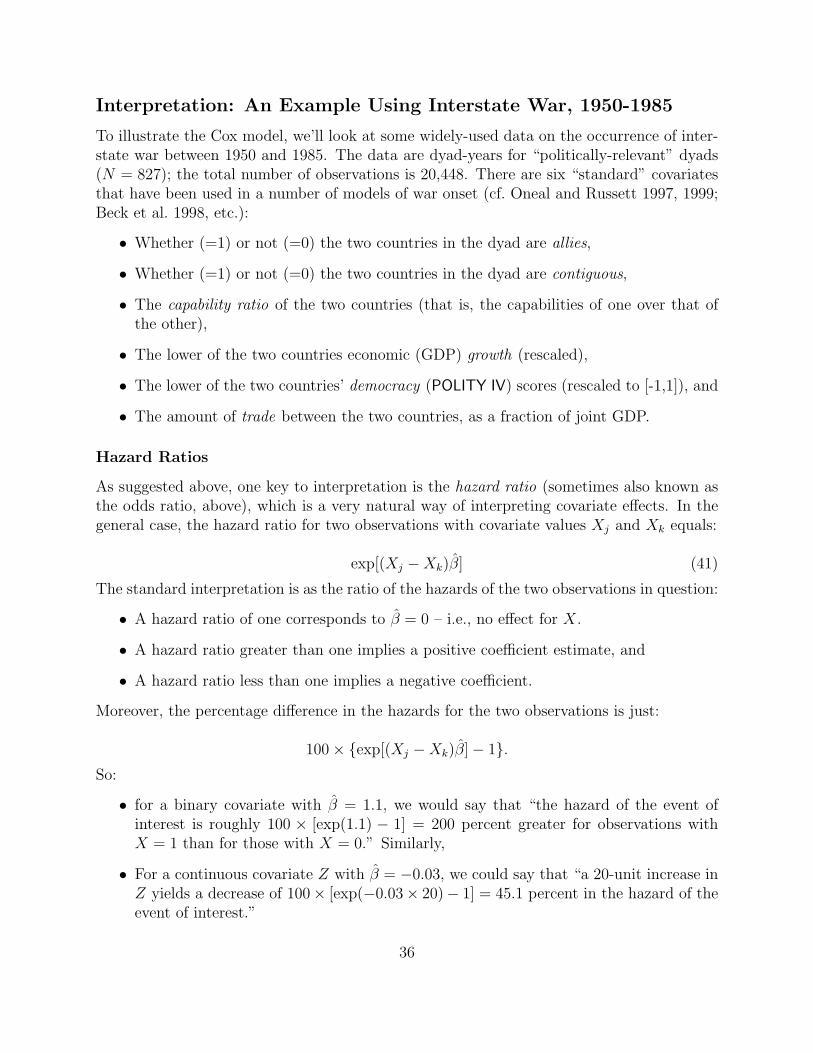
Interpretation: An Example Using Interstate War, 1950-1985

To illustrate the Cox model, we’ll look at some widely-used data on the occurrence of inter-state war between 1950 and 1985. The data are dyad-years for “politically-relevant” dyads(N = 827); the total number of observations is 20,448. There are six “standard” covariatesthat have been used in a number of models of war onset (cf. Oneal and Russett 1997, 1999;Beck et al. 1998, etc.):

• Whether (=1) or not (=0) the two countries in the dyad are allies,

• Whether (=1) or not (=0) the two countries in the dyad are contiguous,

• The capability ratio of the two countries (that is, the capabilities of one over that ofthe other),

• The lower of the two countries economic (GDP) growth (rescaled),

• The lower of the two countries’ democracy (POLITY IV) scores (rescaled to [-1,1]), and

• The amount of trade between the two countries, as a fraction of joint GDP.

Hazard Ratios

As suggested above, one key to interpretation is the hazard ratio (sometimes also known asthe odds ratio, above), which is a very natural way of interpreting covariate effects. In thegeneral case, the hazard ratio for two observations with covariate values Xj and Xk equals:

exp[(Xj −Xk)β] (41)

The standard interpretation is as the ratio of the hazards of the two observations in question:

• A hazard ratio of one corresponds to β = 0 – i.e., no effect for X.

• A hazard ratio greater than one implies a positive coefficient estimate, and

• A hazard ratio less than one implies a negative coefficient.

Moreover, the percentage difference in the hazards for the two observations is just:

100× {exp[(Xj −Xk)β]− 1}.So:

• for a binary covariate with β = 1.1, we would say that “the hazard of the event ofinterest is roughly 100 × [exp(1.1) − 1] = 200 percent greater for observations withX = 1 than for those with X = 0.” Similarly,

• For a continuous covariate Z with β = −0.03, we could say that “a 20-unit increase inZ yields a decrease of 100× [exp(−0.03× 20)− 1] = 45.1 percent in the hazard of theevent of interest.”

36

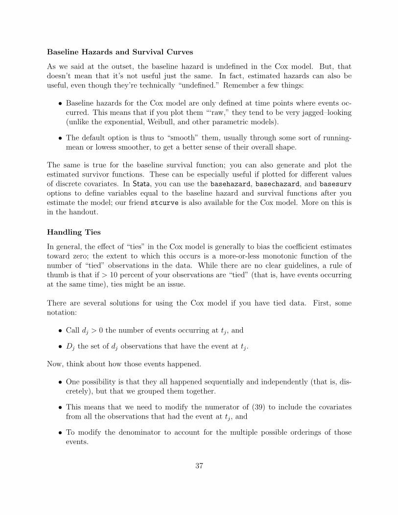
Baseline Hazards and Survival Curves

As we said at the outset, the baseline hazard is undefined in the Cox model. But, thatdoesn’t mean that it’s not useful just the same. In fact, estimated hazards can also beuseful, even though they’re technically “undefined.” Remember a few things:

• Baseline hazards for the Cox model are only defined at time points where events oc-curred. This means that if you plot them “‘raw,” they tend to be very jagged–looking(unlike the exponential, Weibull, and other parametric models).

• The default option is thus to “smooth” them, usually through some sort of running-mean or lowess smoother, to get a better sense of their overall shape.

The same is true for the baseline survival function; you can also generate and plot theestimated survivor functions. These can be especially useful if plotted for different valuesof discrete covariates. In Stata, you can use the basehazard, basechazard, and basesurv

options to define variables equal to the baseline hazard and survival functions after youestimate the model; our friend stcurve is also available for the Cox model. More on this isin the handout.

Handling Ties

In general, the effect of “ties” in the Cox model is generally to bias the coefficient estimatestoward zero; the extent to which this occurs is a more-or-less monotonic function of thenumber of “tied” observations in the data. While there are no clear guidelines, a rule ofthumb is that if > 10 percent of your observations are “tied” (that is, have events occurringat the same time), ties might be an issue.

There are several solutions for using the Cox model if you have tied data. First, somenotation:

• Call dj > 0 the number of events occurring at tj, and

• Dj the set of dj observations that have the event at tj.

Now, think about how those events happened.

• One possibility is that they all happened sequentially and independently (that is, dis-cretely), but that we grouped them together.

• This means that we need to modify the numerator of (39) to include the covariatesfrom all the observations that had the event at tj, and

• To modify the denominator to account for the multiple possible orderings of thoseevents.

37

A simple way to do this is like:

LBreslow(β) =N∏

i=1

exp[(∑

q∈DjXq

)β]

[∑`∈Rj

exp(X`β)]dj

(42)

This is known as Breslow’s (1974) approximation, and is the standard/default way of dealingwith tied event times in most statistical packages (e.g., Stata; SAS, etc., though not in thesurvival package in R). A modification of this was also suggested by Efron (1977);3 it isgenerally accepted that Efron’s is a better approximation than Breslow’s, which is probablywhy it is the default way of dealing with ties in the survival package in R.

Finally, we can use “exact” methods, which take into account that, if there are d events att, then there are d! possible orderings of those events. This approach yields the exact partiallikelihood and exact marginal likelihood methods; they are the most complex, but also themost “accurate,” mathematically speaking.

Some Practical Advice About Ties in the Cox Model

In every case, the approximations reduce to the “standard” Cox partial likelihood when thereare no ties (i.e., when dj = 1∀ j).

• This means that, if there are few ties, all of them will give very similar results.

• So, in that case, there is nothing to worry about.

If you have a lot of ties, things can get a bit dicier. A few rules:

• The Breslow approximation is the “worst.”

• The Efron one is better.

• The exact methods are very computationally demanding, but give the “best” results.However, they can take forever to converge, and (especially in R) may lead to yourmachine freezing up. Be warned.

Generally, using Efron is OK; but use the exact method if you have lots of ties.

3I’m omitting the equation for the Efron approximation here; it’s Eq. (3.35) in Hosmer and Lemeshow(1999) if you really care that much.

38

Software Matters

The Cox Model in Stata

Unsurprisingly, Stata will estimate Cox semiparametric hazard models. The basic commandis stcox, which is similar to streg in a number of ways:

• Before using stcox, the data must be stset,

• As with streg, stcox does not take a “dependent variable” immediately after thecommand,

• A number of post-estimation commands, including stcurve, are allowed after stcox.

As we’ll see a bit later, there are also a large variety of diagnostic commands available forthe Cox model in Stata – we’ll talk about those in a bit.

The Cox Model in R

The basic routine in the survival package is coxph, or, alternatively, cph in the design

package. In contrast to the parametric models, R is fantastic for estimating, diagnosing, andinterpreting Cox models – arguably better than Stata is.

Basic Commands

• coxph in survival

• cph in design

• Both work similarly...

cph and coxph output a proportional hazards regression object, which has a number of usefulcomponents.

Graphing Results

... can be done using plot(survfit()) on the resulting PH object. See the handout for anexample.

39

Discrete-Time Methods

Models for discrete duration data were certainly once – and, in many fields, remain – themost commonly-used approach for analyzing survival data. Discrete-time methods start withan intuitive presence: we are interested in an event, and we can collect data – both acrossunits and over time – on if an when that event happened and relate it to covariates. Thebasic intuition, then, is a more-or-less standard GLM-type model, of the form:

Pr(Yit = 1) = f(Xitβ + uit) (43)

Something like this is the basis for nearly all discrete-time models, which is what we’ll talkabout today.

Concepts

A discrete duration process is one for which the hazard function h(t) is defined only atsome finite or countably infinite set of points in time. Some durations are just discrete. Box-Steffensmeier and Jones discuss Congressional careers in this respect. Alternatively, considera study that focused on confirmation in the Catholic Church:

• Confirmation typically occurs between ages 13-18.

• But it takes a year to get through it. So,

• ...it is essentially discrete: occurs at either age 13 or age 14 or age 15 or ...

• We might want to model this as a function of church-related factors, etc.

One could think of these as being ranked, ordinal categories, in the sense that if you don’t doit at 13, you might at 14, etc. But there are a discrete (and, here, relatively small) numberof possible “times.”

In similar fashion, there are many problems where, at some point, finer-grained time datajust don’t make sense; that is, the durations are effectively discrete. House members’ positionannouncements on the Clinton impeachment (cf. Caldeira and Zorn 2004) is a good exam-ple: There was essentially one week in which members announced, but at what level oughtwe measure the data? Days? Hours? Minutes? Seconds? At some point, the additionalinformation simply isn’t telling us anything valuable.

Other times, we have effectively continuous data that are grouped, and in the process are“discretized.” Of course, all duration data are grouped at some level; the question is whetherthe grouping is sufficiently imprecise to call into question whether we can still think of theresponse variable as continuous. In those instances, there may be some advantages to usingdiscrete-time methods – for example, if the discretization is the result of imprecision in ourmeasuring instrument, such that assuming a continuous-time process implies that we havemuch more information about the process than we really do.

40

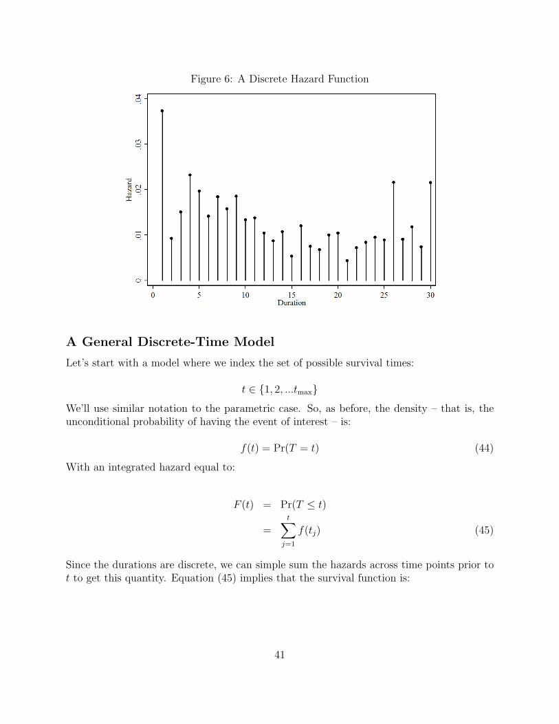
Figure 6: A Discrete Hazard Function

A General Discrete-Time Model

Let’s start with a model where we index the set of possible survival times:

t ∈ {1, 2, ...tmax}

We’ll use similar notation to the parametric case. So, as before, the density – that is, theunconditional probability of having the event of interest – is:

f(t) = Pr(T = t) (44)

With an integrated hazard equal to:

F (t) = Pr(T ≤ t)

=t∑

j=1

f(tj) (45)

Since the durations are discrete, we can simple sum the hazards across time points prior tot to get this quantity. Equation (45) implies that the survival function is:

41

S(t) ≡ Pr(T ≥ t)

= 1− F (t)

=tmax∑j=t

f(tj) (46)

This yields a hazard (i.e., the conditional probability of experiencing the event of interest)equal to:

h(t) ≡ Pr(T = t|T ≥ t)

=f(t)

S(t)(47)

Now, consider an observation that has survived to time t. Because, at time t, you eitherexperience the event or you don’t, the conditional probability of survival at t is:

Pr(T > t|T ≥ t) = 1− h(t) (48)

which means that we can rewrite the conditional probability of survival as the product ofthe previous probabilities of surviving up to that point:

S(t) = Pr(T > t|T ≥ t)× Pr(T > t− 1|T ≥ t− 1)× Pr(T > t− 2|T ≥ t− 2)× ...

×Pr(T > 1|T ≥ 2)× Pr(T > 1|T ≥ 1)

= [1− h(t)]× [1− h(t− 1)]× [1− h(t− 2)]× ...× [1− h(2)]× [1− h(1)]

=t∏

j=0

[1− h(t− j)] (49)

Combining this with (47) we can rewrite the density f(t) in terms of these conditional priorprobabilities:

f(t) = h(t)S(t)

= h(t)× [1− h(t− 1)]× [1− h(t− 2)]× ...× [1− h(2)]× [1− h(1)]

= h(t)t−1∏j=1

[1− h(t− j)] (50)

An observational unit that experiences the event of interest in period t has Yit = 1 in thatperiod, and t− 1 periods of Yit = 0 prior to that. Each of these “observations” thus tells us

42

something about the observation’s (conditional) hazard and survival functions, in a manneranalogous to that for the continuous-time case:

L =N∏

i=1

{h(t)

t−1∏j=1

[1− h(t− j)]

}Yit{

t∏j=0

[1− h(t− j)]

}1−Yit

(51)

This is a general likelihood, in that (at least at this point) it isn’t distribution-specific. Themodel we get, of course, depends on the distribution we chose for the density f(t), as it didin the parametric case.

Approaches to Discrete-Time Data

There are a number of ways for analyzing discrete-time duration data in a GLM-like frame-work.

Ordered-Categorical Models

Suppose we have discrete time data on Ti – that is, the actual survival times in our data –and that the number of those event times K is small. Indexing event times as k ∈ {1, 2, ...K},we can model the resulting duration as an ordered probit or logit, e.g.:

Pr(Ti ≤ k) =exp(τk −Xiβ)

1 + exp(τk −Xiβ)(52)

which is sometimes written as:

ln

[Pr(Ti ≤ κ)

Pr(Ti > κ)

]= τκ −Xiβ (53)

Note:

• This approach was (first?) suggested by Han and Hausman (1990).

• It is an approach that has some nice properties:

◦ It maintains the intrinsic ordering/sequence of the events.

◦ It is relatively easy/straightforward to do and interpret.

◦ It allows for the “spacing” of the events to differ, and be estimated, through theτs.

◦ Finally, it will probably give better estimates than the Cox if there are few eventtimes (and therefore lots of ties).

• However, it also has all the potential pitfalls of ordered logit:

◦ Covariates have the same effect across events (that is, the model maintains theproportional odds / “parallel regressions” assumption, though this can be relaxed).

43

◦ This model also requires a parametric assumption (though this effect is oftenpretty minimal).

◦ Finally, it is difficult (read: impossible) to handle time-varying covariates in sucha setup.

The point of all this is that you can model a duration using an ordered logit/probit, thoughit isn’t done much – I know of one published example in the social sciences...

Grouped-Data (“BTSCS”) Approaches

The more common means of analyzing duration data in a discrete-time framework is bydirectly modeling the binary event indicator. Beck et al. (1998) (hereinafter BKT) refer tothis as “binary time-series cross-sectional” (“BTSCS”) data. The idea is to start with amodel of the probability of an event occurring:

Pr(Yit = 1) = f (Xitβ)

and then apply standard GLM techniques to these data. The most commonly used “link”functions here are the ones we’re all familiar with:

• The logit:

Pr(Yit = 1) =exp(Xitβ)

1 + exp(Xitβ)(54)

• The probit:

Pr(Yit = 1) = Φ(Xitβ) (55)

• The complimentary log-log:

Pr(Yit = 1) = exp[−exp(Xitβ)] (56)

There has been a lot of applied work done using this sort of approach, in political science(Berry and Berry, Mintrom, Squire, BKT, etc.) and in sociology (Allison, Grattet et al.,etc.). In large part, this is because it is easy to do; as a practical matter, one simply:

• Organizes the data by unit/time point,

• Models the binary event (1) / no event (0) variable as a function of the covariates Xusing logit/probit/whatever, and

• Deals with issues like duration dependence on the right-hand side of the model.

44

Advantages

• Models like this are easily estimated, interpreted and understood by readers.

• There are natural interpretations for estimates:

◦ The constant term is akin to the “baseline hazard,” and

◦ Covariates shift this up or down.

• The model can incorporate data in time-varying covariates, which is also a big plus.

• There are lots of software packages that will provide parameter estimates.

(Potential) Disadvantages

• A mode like this requires time-varying data in order to capture the duration element(one may not always have time-varying data in practice). One can, of course, alwaysmake one’s data time-varying by “expanding” it, but if there is no additional informa-tion in the time-varying data (that is, if all the Xs are constant over time), then oneruns the risk of underestimating standard errors and confidence intervals.

• This approach also requires that the analyst takes explicit consideration of the influenceof time, a topic to which we now turn.

Temporal Issues in Grouped-Data Models

It is important to remember that simply estimating a (say) logit on BTSCS data takes noaccount of the possibility of time dependence in the event of interest. Consider (for example)a monthly survey of cohabitating couples, to see when (if) they get married.

• A simple logit treats all the observations on a single couple as the same (that is, asexchangeable).

• More specifically, it doesn’t take the ordering of them into account.

• Implicitly, this is like saying that (all else equal) the hazard of them getting married isthe same in the first month of their living together as it is in the tenth, or the thirtieth.

Statistically, this is equivalent to something akin to an exponential model (independent eventarrivals = memoryless process). We can see this if we consider the “baseline” hazard forsuch a model:

h0(t) =exp(β0)

1 + exp(β0)

45

which is a constant term vis-‘a-vis time. As we said when we discussed parametric models,this assumption is, in most circumstances, an insane one to make.

If we want to get away from this in a grouped-data context, we need to explicitly introducevariables into the covariates to capture changes over time.

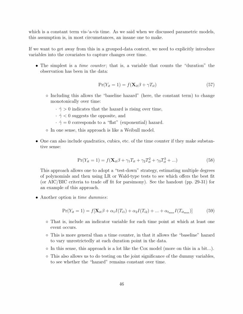
• The simplest is a time counter ; that is, a variable that counts the “duration” theobservation has been in the data:

Pr(Yit = 1) = f(Xitβ + γTit) (57)

◦ Including this allows the “baseline hazard” (here, the constant term) to changemonotonically over time:

· γ > 0 indicates that the hazard is rising over time,

· γ < 0 suggests the opposite, and

· γ = 0 corresponds to a “flat” (exponential) hazard.

◦ In one sense, this approach is like a Weibull model.

• One can also include quadratics, cubics, etc. of the time counter if they make substan-tive sense:

Pr(Yit = 1) = f(Xitβ + γ1Tit + γ2T2it + γ3T

3it + ...) (58)

This approach allows one to adopt a “test-down” strategy, estimating multiple degreesof polynomials and then using LR or Wald-type tests to see which offers the best fit(or AIC/BIC criteria to trade off fit for parsimony). See the handout (pp. 29-31) foran example of this approach.

• Another option is time dummies :

Pr(Yit = 1) = f [Xitβ + α1I(Ti1) + α2I(Ti2) + ... + αtmaxI(Titmax)] (59)

◦ That is, include an indicator variable for each time point at which at least oneevent occurs.

◦ This is more general than a time counter, in that it allows the “baseline” hazardto vary unrestrictedly at each duration point in the data.

◦ In this sense, this approach is a lot like the Cox model (more on this in a bit...).

◦ This also allows us to do testing on the joint significance of the dummy variables,to see whether the “hazard” remains constant over time.

46

This last approach by far the most flexible, but also means (potentially) lots of dummyvariables eating up degrees of freedom. This latter concern is why BKT use cubic splines(smooth functions of the time-dummy variables), the adoption of which has subsequentlybecome a shibboleth among people doing this kind of analysis.

In point of fact, there are a gazillion (that’s a technical term) ways to get around the loss ofdegrees of freedom associated with the dummy-variables approach, cubic splines being onlyone of them. Others include:

• Using higher-order polynomials of survival time, or functions of fractional polynomials,

• Using something like a kernel smoother on the duration

• Including loess or lowess fits of the binary response variable to the survival duration,

• Using other kinds of splines to smooth the survival time variable (B-splines, P-splines,natural splines, etc.).

The handout shows how (e.g.) a lowess fit and the linear predictor from a cubic spline areeffectively identical when it comes to capturing the shape of the underlying hazard in themilitarized interstate dispute (MID) data. Moreover, the models’ fits are all almost exactlythe same.

Discrete-Time Model Selection

Choosing among the possible range of models offered here can be tough. Once again, consider(in order of importance):

1. Theory,

2. formal tests, and

3. fitted values.

The lnLs, AICs, and BICs for the various MID models are:

47

Table 2: AIC and BIC Values, Discrete-Time (Logit) Models

Model lnL d.f. AIC BICNo Dependence / “Flat” -1846.88 7 3707.8 3763.2Linear -1831.75 8 3679.5 3742.9Polynomial -1821.76 11 3665.5 3752.7“Duration Dummies” -1801.31 40 3682.6 3999.7Lowess -1822.75 8 3661.5 3724.9Cubic Spline (linear predictor) -1822.20 8 3660.4 3723.8Cubic Splines -1822.02 10 3664.0 3743.3

If we’re sticking simply to tests for model selection, then both the AIC and the BIC seem toshow a preference for the models incorporating the lowess and linear-predictor cubic splinefunctions of time. On pure log-likelihood terms, however, the dummy-variables model winshands down.

Finally, note that in the discrete-time approach the fact that time dependence is an explicitcovariate means that one can also interact other variables with survival time, to see if (forexample) the effect of a covariate on the probability of the event increases or decreases overtime. We’ll talk more about this tomorrow.

Some Interesting/Useful Equivalencies

The Cox Model and Conditional Logit

In their book, Box-Steffensmeier and Jones discuss the “equivalency” between a (particularform of the) Cox model and a conditional logit model on the Yit event indicator. The intuitionbehind this is that the conditional logit model can be thought of as a model of choice byindividual i from a choice set j ∈ {1, 2, ...J}, of the form:

Pr(Yi = j) =exp(Xijβ + Zjγ)∑J`=1 exp(Xi`β + Z`γ)

(60)

in which the Zjγ – that is, the choice-specific covariates – are “conditioned” out of the model,in a manner akin to “fixed effects,” yielding:

Pr(Yi = j) =exp(Xijβ)∑J`=1 exp(Xi`β)

(61)

These are sometimes also referred to as logit for “matched case-control data,” where thematching is on observations in a choice set.

In the context of duration data, rather than considering the j as being choices from amonga set of options, we can instead think of them as the observations in the “risk set,” and

48

thus having the potential of being “chosen” by the event process to experience the event ofinterest. Remember that, in the Cox model, we had:

Lk =exp(Xkβ)∑

`∈Rjexp(X`β)

. (62)

In this light, it becomes apparent that the Cox model is equivalent to a particular form ofthe conditional logit model, one in which the denominator reflects the various combinationsof potential event orderings that might have happened at a given (discrete) survival time.In that sense, a slightly modified version of the conditional logit estimator is one form of an“exact” semiparametric partial-likelihood model for discrete survival data.

That is all well and good, but – that said – it is not entirely clear to me why we should care.In fact, the only application I’ve seen of this is in Jan & Brad’s book. That’s fine, but I’mnot sure that this is something that is going to take the world by storm.

Cox-Poisson Equivalence

The discussion above about the use of time-dummies leads us to another interesting (andvery important) fact:

Grouped-data duration models and the continuous-time Cox models areequivalent.

That is, it is possible to:

• Use a grouped-duration approach to estimate the parameters of a Cox model, and

• Generate the same baseline hazards, survival functions, and so forth from both models.

Why? How?

The answer lies at the intersection of the Cox model’s form for the survival function and the“counting process” formulation for such models that we talked about yesterday. Recall thatearlier, we noted (in passing) that, for the Cox model:

Si(t) = exp

[−exp(Xiβ)

∫ t

0

h0(t) dt

]In words, this means that the survival function for the Cox model is a complimentary log-logfunction of the covariates X and the (cumulative) baseline hazard – the latter of which isundefined, according to the Cox model.

Now, recall that the probability distribution function for the Poisson is:

49

Pr(Y = y) =exp(−λ)λy

y!

where we normally introduce covariates as λi = exp(Xiβ).

Think about the counting process idea we talked about before. In that case, the variable ofinterest (here, the event indicator Yit) is either equal to zero or one. For the Poisson, theprobability of a zero is:

Pr(Yit = 0) = exp(−λ)

= exp[−exp(Xiβ)]

In this context, Yit = 0 denotes the unconditional survival probability (that is, the absenceof the event of interest), which in turn means that (at t) 1 − exp[−exp(Xiβ)] is the eventprobability. Thus, the key difference between the kernel of the Cox partial likelihood andthe Poisson’s is just the “baseline” hazard; so long as that baseline hazard does not have aspecific form imposed on it, the two are equivalent.

In the Poisson context, not imposing a form on the “baseline” hazard means that we have toallow it to vary unrestrictedly at every event time in the data – in other words, we need toadopt a “dummy-variable” approach to dealing with time dependence. If and when we dothat, the Poisson model is exactly equivalent to the Cox model (albeit the Breslow-for-tiesversion). The handout has an illustration of this equivalency on p. 35.

In practice, this means that estimating a Poisson model on the binary event indicator, andincluding a series of dummy variables for each time point in the model, will yield precisely thesame estimates as the Cox model. At one time, we cared about this because it allowed us touse GLM software to estimate a Cox model. The more important thing about this fact nowis that it means we can use some of the advances that have been developed for event-countmodels in a survival-analysis context, something we will come back to tomorrow.

50

Appendix: Using -stcurve-

Figure 6:

. stcurve, surv

Figure 7:

. stcurve, hazard at1(LatinAm=0 EEurCentAs=0 LatAmxPeer=0 EECAxPeer=0)

at2(peerprivat=11.492 LatinAm=1 LatAmxPeer=11.492 EEurCentAs=0 EECAxPeer=0)

at3(peerprivat=6.351 EEurCentAs=1 EECAxPeer=6.351 LatinAm=0 LatAmxPeer=0)

ytitle(Predicted Survival Probability) xtitle(Time in Years) caption(, size(zero))

legend(order(1 "OECD" 2 "Latin America" 3 "Eastern Europe/Central Asia"))

lp(solid dash dot) lc(black black black) title(, color(white) size(zero))

Figure 8 (same as Figure 7, but with survival):

. stcurve, survival at1(LatinAm=0 EEurCentAs=0 LatAmxPeer=0 EECAxPeer=0)

at2(peerprivat=11.492 LatinAm=1 LatAmxPeer=11.492 EEurCentAs=0 EECAxPeer=0)

at3(peerprivat=6.351 EEurCentAs=1 EECAxPeer=6.351 LatinAm=0 LatAmxPeer=0)

ytitle(Predicted Survival Probability) xtitle(Time in Years) caption(, size(zero))

legend(order(1 "OECD" 2 "Latin America" 3 "Eastern Europe/Central Asia"))


Figure 9:

. stcurve, survival at1(peerprivat=0 LatinAm=1 EEurCentAs=0 LatAmxPeer=0

EECAxPeer=0) at2(peerprivat=10.297 LatinAm=1 LatAmxPeer=10.297

EEurCentAs=0 EECAxPeer=0) at3(peerprivat=31.3 LatinAm=1

LatAmxPeer=31.3 EEurCentAs=0 EECAxPeer=0) ytitle(Predicted Survival

Probability) xtitle(Time in Years) caption(, size(zero)) legend(order(1 "Zero

Peer Privatization" 2 "Mean Peer Privatization" 3 "+2 s.d. Peer Privatization"))


Figure 10:

. stcurve, hazard recast(line) lcolor(black) lpattern(solid) lwidth(medthick)

addplot(scatter basich duration, msymbol(smcircle) mcolor(black)

msize(small)) ytitle(Predicted Hazard) yscale(range(.004 .025))

ylabel(.004(.004).024) xtitle(Time) title(, size(zero) color(white))

Figure 11:

. stcurve, survival at1(allies=0) at2(allies=1) recast(line)

lcolor(black black) lwidth(medthick medthick) lp(dash solid)

ytitle(Estimated Baseline Survival Function) xtitle(Years)

title(, size(zero) color(white)) legend(order(1 "Non-Allies" 2 "Allies"))

51

An Introduction to Event History...

Documents

Transcript of An Introduction to Event History...