An Introduction to Empirical Modeling - Whitman...

An Introduction to Empirical Modeling

Douglas Robert HundleyMathematics Department

Whitman College

September 8, 2014

Contents

1 Basic Models, Discrete Systems 71.1 Introduction . . . . . . . . . . . . . . . . . . . . . . . . . . . . . . 71.2 What Kinds of Models Are There? . . . . . . . . . . . . . . . . . 81.3 Discrete Dynamical Systems . . . . . . . . . . . . . . . . . . . . . 11

2 A Case Study in Learning 192.1 A Case Study in Learning . . . . . . . . . . . . . . . . . . . . . . 192.2 The n−Armed Bandit . . . . . . . . . . . . . . . . . . . . . . . . 20

3 Statistics 333.1 Functions that Define Data . . . . . . . . . . . . . . . . . . . . . 333.2 The Mean, Median, and Mode . . . . . . . . . . . . . . . . . . . 363.3 The Variance and Standard Deviation . . . . . . . . . . . . . . . 393.4 The Covariance Matrix . . . . . . . . . . . . . . . . . . . . . . . . 423.5 Exercises . . . . . . . . . . . . . . . . . . . . . . . . . . . . . . . 423.6 Linear Regression . . . . . . . . . . . . . . . . . . . . . . . . . . . 453.7 The Median-Median Line: . . . . . . . . . . . . . . . . . . . . . . 48

4 Linear Algebra 514.1 Representation, Basis and Dimension . . . . . . . . . . . . . . . . 534.2 Special Mappings: The Projectors . . . . . . . . . . . . . . . . . 564.3 The Four Fundamental Subspaces . . . . . . . . . . . . . . . . . . 594.4 Exercises . . . . . . . . . . . . . . . . . . . . . . . . . . . . . . . 614.5 The Decomposition Theorems . . . . . . . . . . . . . . . . . . . . 634.6 Interactions Between Subspaces and the SVD . . . . . . . . . . . 73

I Data Representations 77

5 The Best Basis 795.1 The Karhunen-Loeve Expansion . . . . . . . . . . . . . . . . . . 795.2 Exercises: Finding the Best Basis . . . . . . . . . . . . . . . . . . 805.3 Connections to the SVD . . . . . . . . . . . . . . . . . . . . . . . 835.4 Computation of the Rank . . . . . . . . . . . . . . . . . . . . . . 84

3

4 CONTENTS

5.5 Matlab and the KL Expansion . . . . . . . . . . . . . . . . . . . 855.6 The Details . . . . . . . . . . . . . . . . . . . . . . . . . . . . . . 875.7 Sunspot Analysis, Part I . . . . . . . . . . . . . . . . . . . . . . . 895.8 Eigenfaces . . . . . . . . . . . . . . . . . . . . . . . . . . . . . . . 905.9 A Movie Data Example . . . . . . . . . . . . . . . . . . . . . . . 98

6 A Best Nonorthogonal Basis 1016.1 Set up the Signal Separation Problem . . . . . . . . . . . . . . . 1026.2 Signal Separation of Voice Data . . . . . . . . . . . . . . . . . . . 1066.3 A Closer Look at the GSVD . . . . . . . . . . . . . . . . . . . . . 108

7 Local Basis and Dimension 111

8 Data Clustering 1138.1 Background . . . . . . . . . . . . . . . . . . . . . . . . . . . . . . 1138.2 The LBG Algorithm . . . . . . . . . . . . . . . . . . . . . . . . . 1178.3 K-means Clustering via SVD . . . . . . . . . . . . . . . . . . . . 1208.4 Kohonen’s Map . . . . . . . . . . . . . . . . . . . . . . . . . . . . 1208.5 Neural Gas . . . . . . . . . . . . . . . . . . . . . . . . . . . . . . 1268.6 Clustering and Local KL . . . . . . . . . . . . . . . . . . . . . . . 1338.7 A Comparison of the Techniques . . . . . . . . . . . . . . . . . . 138

II Functional Representations 141

9 Linear Neural Networks 1439.1 Introduction and Notation . . . . . . . . . . . . . . . . . . . . . . 1439.2 Training a Linear Net . . . . . . . . . . . . . . . . . . . . . . . . 1469.3 Time Series and Linear Networks . . . . . . . . . . . . . . . . . . 1519.4 Script file: APPLIN2 . . . . . . . . . . . . . . . . . . . . . . . . . 1539.5 Matlab Demonstration . . . . . . . . . . . . . . . . . . . . . . . . 1559.6 Summary . . . . . . . . . . . . . . . . . . . . . . . . . . . . . . . 155

10 Radial Basis Functions 15710.1 The Process of Function Approximation . . . . . . . . . . . . . . 15710.2 Using Polynomials to Build Functions . . . . . . . . . . . . . . . 15810.3 Distance Matrices . . . . . . . . . . . . . . . . . . . . . . . . . . . 16310.4 Radial Basis Functions . . . . . . . . . . . . . . . . . . . . . . . . 16610.5 Orthogonal Least Squares . . . . . . . . . . . . . . . . . . . . . . 17410.6 Homework: Iris Classification . . . . . . . . . . . . . . . . . . . . 178

11 Neural Networks 18111.1 From Biology to Construction . . . . . . . . . . . . . . . . . . . . 18111.2 History and Discussion . . . . . . . . . . . . . . . . . . . . . . . . 18511.3 Training and Error . . . . . . . . . . . . . . . . . . . . . . . . . . 18711.4 Neural Networks and Matlab . . . . . . . . . . . . . . . . . . . . 19011.5 Post Training Analysis . . . . . . . . . . . . . . . . . . . . . . . . 196

CONTENTS 5

11.6 Example: Alphabet recognition . . . . . . . . . . . . . . . . . . . 19911.7 Project 1: Mushroom Classification . . . . . . . . . . . . . . . . . 20011.8 Autoassociation Neural Networks . . . . . . . . . . . . . . . . . . 201

III Time and Space 205

12 Fourier Analysis 20712.1 Introduction . . . . . . . . . . . . . . . . . . . . . . . . . . . . . . 20712.2 Implementation of the Fourier Transform . . . . . . . . . . . . . 21012.3 Applying the FFT . . . . . . . . . . . . . . . . . . . . . . . . . . 21612.4 Short Term Fourier and Windowing . . . . . . . . . . . . . . . . 22512.5 Fourier and Biological Mechanisms . . . . . . . . . . . . . . . . . 22712.6 Chapter Summary . . . . . . . . . . . . . . . . . . . . . . . . . . 228

13 Wavelets 229

14 Time Series Analysis 231

IV Appendices 233

A An Introduction to Matlab 235

B The Derivative 251B.1 The Derivative of f . . . . . . . . . . . . . . . . . . . . . . . . . . 251B.2 Worked Examples: . . . . . . . . . . . . . . . . . . . . . . . . . . 255B.3 Optimality . . . . . . . . . . . . . . . . . . . . . . . . . . . . . . 256B.4 Worked Examples . . . . . . . . . . . . . . . . . . . . . . . . . . 259B.5 Exercises . . . . . . . . . . . . . . . . . . . . . . . . . . . . . . . 260

C Optimization 263

D Matlab and Radial Basis Functions 265

V Bibliography 271

VI Index 277

6 CONTENTS

Chapter 1

Basic Models, DiscreteSystems

1.1 Introduction

Mathematical modeling is the process by which we try to express physical pro-cesses mathematically. In so doing, we need to keep some things in mind:

• What are our assumptions?

That is, what assumptions are absolutely necessary for us to emulate thedesired behavior? For example, we might be interested in the fluctuationof a population. In that situation, we may or may not want to changesbased on seasonality.

• The model should be simple enough so that we can understand it. If amodel is so complicated as to defy understanding, then the model is notuseful.

• The model should be complex enough so that we capture the desiredbehavior. The model should not be so simple that it does not explainanything- again, such a model is not useful. This does not mean that weneed a lot of equations, however. One of the lessons of chaos theory1 isthe following:

Very simple models can create very complex behavior

• To put the previous two items into context, when we build a model, weprobably have some questions in mind that we’d like to answer. You canevaluate your model by seeing if it gives you the answer- For example,

1For a general introduction to Chaos Theory, consider reading “Chaos”, by James Gleick.For a mathematical introduction, see “An Introduction to Chaotic Dynamics”, by RobertDevaney

7

8 CHAPTER 1. BASIC MODELS, DISCRETE SYSTEMS

– Should a stock be bought or sold?

– Is the earth becoming warmer?

– Does creating a law have a positive or negative social effect?

– What is the most valuable property in monopoly?

In this way, a model provides added value, and it is by this property thatwe might evaluate the goodness of a model.

• Once a model has been built, it needs to be checked against reality- Mod-eling is not a thought experiment! Of course, you would then go back toyour assumptions, and revise, create new experiments, and check again.

You might notice that we have used very subjective terms in our definitionof “modeling”- and these are an intrinsic part of the process. Some of the mostbeautiful and insightful models are those that are elegant in their simplicity.Most everyone knows the following model, which relates energy to mass and thespeed of light:

E = mc2

While it is simple, the model is also far-reaching in its implications (we willnot go into those here). Other models of observed behavior from physics areso fundamental, we even call them physical “laws”- such as Newton’s Laws ofMotion.

In building mathematical models, you are allowed and encouraged to be cre-ative. Explore and question your assumptions, explore your options for express-ing those options mathematically, and most importantly, use your mathematicalbackground.

1.2 What Kinds of Models Are There?

There are many ways of classifying mathematical models, which will make senseonce you begin to build your own models. In general, we might consider thefollowing classes of models:

1.2.1 Deterministic vs. Stochastic

A stochastic model is one that uses random variation. To describe this randomvariation properly, we will typically need ideas from statistics. An example:Model the outcomes of a roll of dice. Stochastic models are characterized bythe introduction of statistics and probability. We won’t be doing a lot of thisin our course.

On the other hand, in a deterministic model, there is no randomness. Asan example, we might model the temperature of a cup of coffee as it variesover time (a cooling model). Classically, the model would only involve thetemperature of the coffee and the temperature of the environment.

1.2. WHAT KINDS OF MODELS ARE THERE? 9

There may not be a clean division of categories here; it is common for somemodels to incorporate both deterministic and stochastic parts. For example, amodel for a microphone may include a model for the voice (deterministic), anda model for noise (stochastic).

It is interesting to consider the following: Does a deterministic model neces-sarily produce results that are completely predictable through all time? Inter-estingly, the answer is: Maybe yes, Maybe no. Yes, in the theoretical sense- wemight be able to show that there exists a single unique solution to our problem.No, in the practical sense that we might not actually be able to compute thatsolution. However, this does not mean that all is lost- we might have excellentapproximations over a short time span (think of the weather models on thenews).

1.2.2 Discrete vs. Continuous Time

In modeling an occurrence that depends on time, it might happen at discretesteps in time (like interest on my credit card, or population), or in continuoustime (like the temperature at my desk).

Modeling in Discrete Time

Discrete time models usually index time as a subscript- For example, an or xn

will be the value of a or x at time step n.Discrete time models can be defined recursively, like the following:

an+1 = an + an−1

In order to “solve” the system to produce a sequence, we would need to initializethe problem. For example, if a0 = 1 and a1 = 1, then we can find all the otherelements of the sequence:

{1, 1, 2, 3, 5, 8, 13, · · · }

You might recognize this as the famous Fibonacci sequence.

General discrete models

There are a couple of fundamental assumptions being made in these discretemodels: (1) Time is indexed by the integers, and (2) The value of the processat some time n+ 1 is a function of at most a finite number of previous states.

Mathematically, this means, given an and the L previous values of the statea, then the next state at time n+ 1 is given by:

an+1 = f(an, an−1, . . . , an−L)

Or, rather than modeling the states directly, we might model how the statechanges in time:

an+1 − an = Δan = f(an−1, . . . , an−L)


In either event, we will be left with determining the form for the function f andthe length of the past, L. This form is called a difference equation.

We will work with both types of discrete models shortly. Before we do, letus contrast these models with continuous time models.

Modeling in Continuous Time

We may model using Ordinary Differential Equations. In these models, weare assuming that time passes continually, and that the rate of change of thequantity of interest depends only on the quantity and current time. We capturethese assumptions by the following general model, where y(t) is the quantity ofinterest.

dy

dt= f(t, y)

Note that this says simply that the rate of change of the quantity y depends onthe time t and the current value of y.

Let us consider an example we’ve seen in Calculus: Suppose that we assumethat acceleration of a falling body is due only to the force of gravity (we’llmeasure it as feet/sec2). Then we may write:

y�� = −16

We can solve this for y(t) by antidifferentiation:

y� = −16t+ C1, y(t) = −8t2 + C1t+ C2

where C1, C2 are unknowns that are problem-specific. These simples models areusually considered in a first course in ODEs.

To produce a more complex model, we might say that the rate of changedepends not only on the quantity now, but also the value of the quantity in thepast (for example, when regulating bodily functions the brain is reading valuesthat are from the past). Such a model may take the following form, where x(t)denotes the quantity of interest (such as the amount of oxygen in the blood):

dx

dt= f(x(t)) + g(x(t− τ))

This is called a delay differential equation. One of the most famous of thesemodels is the “Mackey-Glass” equation- You might look it up on the internetto see what the solution looks like!

If our phenomena requires more than time, we have to model via PartialDifferential Equations. For example, it is common for a function u(t, x) todepend both on time t and position x. Then a PDE may be:

∂u

∂t= k

∂2u

∂x2

which might be interpreted to read: “The velocity of u at a particular time andposition is proportional to its second spatial derivative. Modeling with PDEs isgenerally done in our Engineering Mathematics course.

1.3. DISCRETE DYNAMICAL SYSTEMS 11

1.2.3 Empirical vs. Analytical Modeling

“Empirical modeling” is modeling directly from data, rather than by some an-alytic process. In this case, our assumptions may take the form of a “modelfunction” to which we will find unknown parameters. You’ve probably seen thisbefore in articles where the researcher is fitting a line to data- in this example,we assume the model equation is given as y = mx + b, where m and b are theunknown parameters.

We’ll finish this chapter with some analytical modeling using discrete dy-namical systems (or, equivalently, discrete difference equations).

1.3 Discrete Dynamical Systems

The simplest type of dynamical system might be written in the following re-currence form (recurrence because we’re writing the next value in terms of thecurrent value):

xn+1 = axn

where we would call x0 the initial condition. So, given x0, we could computethe future values of the dynamical system:

x1 = ax0 x2 = ax1 = a2x0 x3 = ax2 = a3x0 · · ·

The set of values x1, x2, x3, . . . are called the orbit of x0. We also notice thatin this particular example, we were able to express xn in terms of x0. This iscalled the closed form of the solution to the difference equation given. Thatis,

xn = anx0

solves the system: xn+1 = axn. In fact, we can predict the long term behaviorof this system:

|xn| →

0 if |a| < 1∞ if |a| < 1x0 if a = 1

And, if a = −1, the orbit oscillates between ±x0. In this case, we say that ±x0

are periodic with period 2.

Generally, if we have the Lth order difference equation:

xn+1 = f(xn, xn−1, . . . , xn−(L−1))

we would need to know L values of the past. For example, here’s a second orderdifference equation:

xn+1 = xn + xn−1

So, if we have x0 = 1 and x1 = 1, then

x2 = 2, x3 = 3, x4 = 5, x5 = 8, x6 = 13, . . .

This is the Fibonacci sequence. In this case, the orbit grows without bound.


1.3.1 Periodicity

Before continuing, let’s get some more vocab.Given xn+1 = f(xn), a point w is a fixed point of f (or a fixed point for

the orbit of x0) ifw = f(w)

(Because dynamically, that point will never change). Continuing, a point w isa periodic point of order k if

fk(w) = w

The least such k is the prime period. Here’s an example- Find the fixed pointsand period 2 points for the following:

xn+1 = f(xn) = x2n − 1

SOLUTION: The fixed point is found by solving x = f(x):

x2 − 1 = x ⇒ x2 − x− 1 = 0 ⇒ x =1±

√5

2

The period two points are found by solving x = F (F (x)). Notice that we alreadyhave part of the solution (fixed points are also period 2 points).

F (F (x)) = (x2 − 1)2 − 1 = x4 − 2x2

so we solve:x4 − 2x2 = x

which generally can be difficult to solve. However, we can factor out x2 − x− 1and x to factor completely:

x4 − 2x2 − x = 0 ⇒ x(x+ 1)(x2 − x− 1) = 0

Therefore, x = 0 and x = −1 are the prime period 2 points.Points may also be eventually fixed, like x =

√2 for F (x) = x2 − 1. If we

compute the actual orbit, we get√2, 1, 0,−1, 0,−1, . . .

Solving First Order Equations

Consider making the first order sequence slightly more complicated:

xn+1 = axn + b

where a, b are constants (so f(x) = ax + b). Then, given an arbitrary x0, wewonder if we can write the solution in closed form:

x1 = ax0 + b x2 = ax1 + b = a(ax0 + b) + b = a2x0 + ab+ b


For x3, we have:

x3 = a( a2x0 + ab+ b ) + b = a3x0 + a2 + b+ ab+ b

and so on. Therefore, we have the closed form:

xn = anx0 + b(1 + a+ a2 + · · ·+ an−1)

Do we recall how to get the partial (or finite) geometric sum? Back then, wemight have written it this way: Let S be the partial sum. That is,

S = 1 + a+ a2 + . . .+ an−1

aS = a+ a2 + . . .+ an

(1− a)S = 1− anS =

1− an

1− a=

an − 1

a− 1

Given xn+1 = axn + b, the closed form solution is

xn = anx0 + ban − 1

a− 1

and the fixed point is:

ax+ b = x ⇒ (a− 1)x = −b ⇒ x =b

1− a

Notice that we could re-write the closed form in terms of the fixed point:

xn = an�x0 −

b

1− a

�+

b

1− a

EXAMPLE: Discrete Compound of InterestGenerally, if we begin with P0 dollars accruing at an annual interest of r

percent (as a number between 0 and 1), then

Pn+1 =�1 +

r

12

�Pn

If you deposit an additional k dollars each month, you would add k to theprevious amount, and we would have the form F (x) = ax+ b which we studiedin the previous section.

CAUTION: Careful what you use for the interest rate. For example, witha 5% annual interest rate, the number r you see in the formula is 5

100 , so theoverall quantity

1 +r

12= 1 +

5

1200

Example

Suppose that Peter works for 4 years, and during this time he deposits $1000each month on a savings account at an annual interest rate of 5% (with noinitial deposit). During the next 4 years, he withdraws equal amounts p so that


at the end of 4 years, he has a zero balance again. Find p and the total interestearned.

SOLUTION: We’ll treat the two time intervals separately, since the dynamicschange after 4 years. For the first 4 years, we have P0 = 0 and at the end of 4years (n = 48), we have

P48 = ba48 − 1

a− 1

Substituting n = 48, a = 1 + 51200 = 241

200 , and b = 1000, we have:

P48 = $53, 014.89

For the next four years, the dynamical system has the form:

Pn+1 = aPn − k

where the new initial amount is P0 = 53014.89, and k is the amount we’rewithdrawing each month. After 4 years, we have zero dollars exactly:

P48 = 53014.89a48 − ka48 − 1

a− 1= 0 ⇒ k =

a− 1

a48 − 1(53014.89a48) = k

That gives k ≈ $1220.89. For the total interest, Peter has withdrawn 48 ×1220.89 = 58602.72, and he has deposited 48 × 1000 = 48000. Therefore,putting it all together, Peter has made about $10,602.72 in interest.

Exercises

1. You decide to purchase a home with a mortgage at 6% annual interestand with a term of 30 years (assume no down payment). If your housecosts $200,000, what will the monthly payment be? On the other hand,if you can only make $1000 monthly payments, how much of a house canyou afford?

Visualizing First Order Equations

See Ch 4 of the Devaney’s text...Given the form xn+1 = F (xn), and an initial point x0, there is a nice way

to visualize the orbit. Consider the graph of y = F (x). Some observations:

• The points of intersection between y = x and y = F (x) are the fixedpoints of the recurrence.

• If we start with x0 along the “x−axis, then go vertically to the graph, wewill be at the point (x0, x1).

• To find x2, first go horizontally from (x0, x1) to (x1, x1). Then treat x1 asa domain value, and go vertically to the graph of F . The coordinate willnow be (x1, x2).


• Continue this process to visualize the orbit of x0.

From last time, we finished by considering

xn+1 = f(xn)

In this particular instance, we can perform “graphical analysis” by looking atthe graph of y = f(x):

• Include the line y = x; the points of intersection are the fixed points.

• To find the orbit, given a number x0:

– Go vertically to x1 = f(x0). Thus, you are located at the point(x0, x1). We want to use x1 as the next domain point:

– Go horizontally to the line y = x. Thus, you are now located at thepoint (x1, x1), so you can use x1 as a domain value.

– Go vertically to (x1, x2), where x2 = f(x1).

– Go horizontally to (x2, x2).

– Go vertically to (x2, x3)

– And so on...

IN CLASS EXAMPLES: y =√x and y = ax+ b.

We can define attracting, repelling fixed points.Now, before going further, let’s focus again on first and second order differ-

ence equations.

Definition: A difference equation is an equation typically of the form

xn+1 − xn = f(xn−1, . . . , xn−L)

However, we will also see it as a discrete system:

xn+1 = f(xn, . . . , xn−L)

So we’ll refer to either type when discussing difference equations.

Non-homogeneous Difference Equations

Consider now a slightly different form for difference equations:

xn+1 = axn + bn

If bn was actually constant, then we already derived the closed form of thesolution. In this case, we’ll focus on what happens if bn is a function of n.

First, some vocab: If we only consider xn+1 = axn, then that is called thehomogeneous part of the equation. The solution to that we’ve already


determined to be xn = Can (where C depends on the initial condition), andwe’ll refer to this as the homogeneous part of the solution.

If we have a solution pn to the full equation, where bn �= 0, we’ll refer tothat as the particular part of the solution.

We will show that, if pn is any particular solution, then

xn = can + pn

is a solution to the difference equation, and actually solves the DE with arbitrarystarting conditions.

To show that xn is indeed a solution, compute xn+1, then compare withaxn + bn:

xn+1 = can+1 + pn+1

axn + b = a(can + pn) + pn = can+1 + apn + pn

This is a solution as long as pn+1 = apn + pn, which it is. Finding pn canbe challenging, but there are some cases where we can “guess and check”:

Example: Find the general solution to

xn+1 = 3xn + 2n+ 1

SOLUTION: We’ll guess that bn has the same general form as 2n + 1, so weguess

bn = A+Bn

Substituting this back into the difference equation, we have

A+B(n+ 1) = 3(A+Bn) + 2n+ 1 ⇒ A+Bn+B = 3A+ 3Bn+ 2n+ 1

0 = (2A−B + 1) + (2B + 2)n = 0

This equation is true for all n = 1, 2, . . ., so therefore 2B+2 = 0 and 2A−B+1 =0. That lets us solve, B = −1 and A = −1

pn = −(n+ 1)

The general solution:xn = c3n − (n+ 1)

where c is a constant that depends on the initial condition.

Sines and Cosines

We can do something similar for sines and cosines, although we need to usesum/difference formulas that you may not recall:

sin(A+B) = sin(A) cos(B) + sin(B) cos(A)

cos(A+B) = cos(A) cos(B)− sin(A) sin(B)


NOTE: I’ll provide these formulas for quizzes/exams.Here’s an example:

xn+1 = −xn + cos(2n)

The homogeneous part of the solution is c(−1)n. For the particular part, we’llguess that

pn = A cos(2n) +B sin(2n)

and we’ll see if we can solve for A, B. Substituting, we have:

A cos(2(n+ 1)) +B sin(2(n+ 1)) = −A cos(2n)−B sin(2n) + cos(2n)

Using the formulas,

A(cos(2n) cos(2)−sin(2n) sin(2))+B(sin(2n) cos(2)+sin(2) cos(2n)) = −A cos(2n)−B sin(2n)+cos(2n)

Collecting terms, we look at the coefficients of cos(2n) and sin(2n) separately:

cos(2n) [A cos(2) +B sin(2) +A] = cos(2n)

sin(2n) [−A sin(2) +B cos(2) +B] = 0

These equations must be true for each integer n, therefore

A(1 + cos(2)) +B sin(2) = 1−A sin(2) +B(1 + cos(2)) = 0

⇒ A =1

2, B =

sin(2)

2(1 + cos(2))

The overall solution is therefore:

xn = C(−1)n +1

2cos(2n) +

sin(2)

2(1 + cos(2))sin(2n)

EXERCISE: Find the general solution to

xn+1 =1

2xn +

n

2n.

Do this by assuming that the the particular solution is of the form

pn =n(An+B)

2n

Closing Notes

We might notice that solving these difference equations is very similar to solving

Ax = b

in linear algebra, or solving

ay�� + by� + cy = g(t)

in differential equations (the Method of Undetermined Coefficients). This isnot a coincidence- They all rely on the underlying equation being from a linearoperator.

For now, we will close the introduction in order to get an introduction toMatlab.

Chapter 2

A Case Study in Learning

2.1 A Case Study in Learning

In a broad sense, learning is the process of building a “desirable” associationbetween stimulus and response (domain and range), and is measured throughresulting behavior on stimulus that has not been previously seen.

In machine learning, problems are typically cast in one of two models: Eithersupervised or unsupervised learning.

In supervised learning, we are given examples of proper behavior, and wewant the computer to emulate (and extrapolate from) that behavior.

In the other type of learning, unsupervised learning, no specific outputs aregiven per input, but rather an overall goal is given. Here are some examples tohelp with the definition:

• Suppose you have an old clunker of a car that doesn’t have much of anengine. You’re stuck in a valley, and so the only way out will be to go asfast as you can for a while, then let gravity take you back up the otherside of the hill, then accelerate again, and so on. You hope that you canbuild up enough momentum to get out of the valley (that’s the goal).

• Suppose you’re driving a tractor-trailer, and you need to back the trailerinto a loading dock (that’s your goal).

• In a game of chess, the input would be the position of each of the chesspieces. The overall goal is to win the game.

In general, supervised learning is easier than unsupervised learning. Onereason is that in unsupervised learning, a lot of time wasted in trial-and-errorexploration of the possible input space. Contrast that with supervised learning,where the “correct” behavior is explicitly given.

19

20 CHAPTER 2. A CASE STUDY IN LEARNING

2.1.1 Questions for Discussion:

1. Consider the concept of superstition: This is a belief that one must engagein certain behaviors in order to receive a certain reward, where in reality,the reward did not depend on those behaviors. Is it possible for a computerto engage in superstitious activity? Discuss in terms of the supervisedversus unsupervised learning paradigms.

2. A signal light comes on and is followed by one of two other lights. The goalis to predict which of the lights comes on given that the signal light comeson. The experimenter is free to arrange the pattern of the two responselights in any way- for example, one might come on 75% of the time.

Let E1, E2 denote the event that the first (second) light comes on, andlet A1, A2 denote the prediction that the first (second) light comes on(respectively). Let π be the probability that E1 occurs.

(a) If the goal is to maximize your reward through accurate predictions,what should you do in this experiment? Just give a heuristic answer-you do not have to formally justify it.

(b) How would you program a machine to maximize it’s prediction ac-curacy? Can you state this in mathematical terms?

(c) What do you think happens with actual subject (human) trials?

2.2 The n−Armed Bandit

The one armed bandit is slang for a slot machine, so the n−armed bandit canbe thought of as a slot machine with n arms. Equivalently, you may think of aroom with n slot machines.

The problem we’re trying to solve is the classic Las Vegas quandry: Howshould we play the slot machines in order to maximize our returns?

Discussion Question: Is the n−armed bandit a case or supervised or unsu-pervised learning?

First, let us set up some notation: Let a be an integer between 1 and n thatdefines which machine we’re playing. Then define the expected return:

Q(a) = The expected return for playing slot machine a

You can also think of Q(a) as the mean of the payoffs for slot machine a.If we knew Q(a) for each machine a, our strategy to maximize our returns

would be very simple: “Play only machine a”.Of course, what makes the problem interesting is that we don’t know what

the any of the returns are, let alone which machine gives the maximum. Thatleaves us to estimate the returns, and because there will always be uncertainty

2.2. THE N−ARMED BANDIT 21

associated with these estimates, we will never know if the estimates are correct.We hope to construct estimates that get better over time (and experience).

Let’s first set up some notation. Let

Qt(a) = Our estimation of Q(a) at time t.

so we hope that our estimates get better in time:

limt→∞

Qt(a) = Q(a) (2.1)

Suppose we play slot machine a a total of na times, with payoffs r1, . . . , rna

(note that these values could be negative!). Then we might estimate Q(a) asthe mean of these values:

Qt(a) =r1 + r2 + . . .+ rna

na

In statistical terms, we are using the sample mean to estimate the actual meanwhich is a reasonable thing to do as a starting point. We’ll also initialize theestimates to be zero: Q0(a) = 0.

We now come to the big question: What approach should we take to accom-plish our goal (of maximizing our reward). The first one up is a good place tostart.

2.2.1 The Greedy Algorithm

This strategy is straightforward: Always play the slot machine with the largest(estimated) payoff. If at+1 is the machine we’ll play at time t+ 1, then:

at+1 = argmax {Qt(1), Qt(2), . . . , Qt(n)}

where “arg” refers to the argument of the maximum (which is an integer from1 to n corresponding to the max) . If there is a tie, then choose one of them atrandom.

We’ll need to translate this into a learning algorithm, so set’s take a momentto see how we might implement the greedy algorithm in Matlab.

Translating to Matlab

The find and max commands will be used to find the argument of the maxi-mum value. For example, if x is a (row) vector of numbers, then the followingcommand:

idx=find(x==max(x))

will return all indices of the vector x that are equal to the max.Here’s an example. Suppose we have vector x as given. What does Matlab

do?


x=[1 2 3 0 3];

idx=find(x==max(x));

The result will be a vector, idx, that contains the values 3 and 5 (that is, thethird and fifth elements of x are where the maximum occurs).

Going back to the greedy algorithm, I think you’ll see a problem- Whatif the estimations are wrong? Then its very possible that you’ll get stuck ona suboptimal machine. This problem can be dealt with in the following way:Every once in a while, try out the other machines to see what you get. This iswhat we’ll do in the next section.

2.2.2 The �−Greedy Algorithm

In this algorithm, rather than always choosing the machine with the greatestcurrent estimate of the payout, we will choose, with probability �, a machine atrandom.

With this strategy, as the number of trials gets larger and larger, na → ∞for all machines a, and so we will be guaranteed convergence to the properestimates of Q(a) for all a machines.

On the flip side, because we’re always investigating other machines everyonce in a while, we’ll never maximize our returns (we will always have subopti-mal returns).

Implementing epsilon−greedy in Matlab

Using some “pseudo-code”, here is what we want our algorithm to do:

For each time we choose a machine:

• Select an action:

– Sometimes choose a machine at random

– Otherwise, select the action with greatest return. Check

for ties, and if there is a tie, pick on of them at random.

• Get your payoff

• Update the estimates Q

Repeat.

Our first programming problem will be to implement the statement “Some-times choose a machine at random”. If we define � =E to be the probability ofthis event, and N is the number of trials, then one way of selection is to set upa vector with N elements which we’ll call greedy, that will “flag” the events-that is, on trial j, if greedy(j)= 1, choose a machine at random. Otherwise,choose using the greedy method. The following code will do just that (N is thenumber of trials)


greedy=zeros(1,N);

if E>0

m=round(E*N); %Total number of times we should choose at random

greedy(1:m)=ones(1,m);

m=randperm(N); %Randomly permute the vector indices

greedy=greedy(m);

clear m

end

And here’s the full function. We assume that the actual rewards for each ofthe bandits is given in the vector Aq, and that when machine a is played, thesample reward will be chosen from a normal distribution with unit variance andmean Aq(a).

function [As,Q,R]=banditE(N,Aq,E)

%FUNCTION [As,Q,R]=banditE(N,Aq,E)

% Performs the N-armed bandit example using epsilon-greedy

% strategy.

% Inputs:

% N=number of trials total

% Aq=Actual rewards for each bandit (these are the mean rewards)

% E=epsilon for epsilon-greedy algorithm

% Outputs:

% As=Action selected on trial j, j=1:N

% Q are the reward estimates

% R is N x 1, reward at step j, j=1:N

numbandits=length(Aq); %Number of Bandits

ActNum=zeros(numbandits,1); %Keep a running sum of the number of times

% each action is selected.

ActVal=zeros(numbandits,1); %Keep a running sum of the total reward

% obtained for each action.

Q=zeros(1,numbandits); %Current reward estimates

As=zeros(N,1); %Storage for action

R=zeros(N,1); %Storage for averaging reward

%*********************************************************************

% Set up a flag so we know when to choose at random (using epsilon)

%*********************************************************************

greedy=zeros(1,N);

if E>0

m=round(E*N); %Total number of times we should choose at random

greedy(1:m)=ones(1,m);

m=randperm(N);

greedy=greedy(m);

clear m

end

if E>=1

error(’The epsilon should be between 0 and 1\n’);

end


%********************************************************************

%

% Now we’re ready for the main loop

%********************************************************************

for j=1:N

%STEP ONE: SELECT AN ACTION (cQ) , GET THE REWARD (cR) !

if greedy(j)>0

cQ=ceil(rand*numbandits);

cR=randn+Aq(cQ);

else

[val,idx]=find(Q==max(Q));

m=ceil(rand*length(idx)); %Choose a max at random

cQ=idx(m);

cR=randn+Aq(cQ);

end

R(j)=cR;

%UPDATE FOR NEXT GO AROUND!

As(j)=cQ;

ActNum(cQ)=ActNum(cQ)+1;

ActVal(cQ)=ActVal(cQ)+cR;

Q(cQ)=ActVal(cQ)/ActNum(cQ);

end

Next we’ll create a test bed for the routine. We will call the program 2,000times, and each call will consist of 1,000 plays. We will set the number of banditsto 10, and change the value of � from 0 to 0.01 to 0.1, and see what the averagereward per play is over the 1000 plays.

Here’s a script file that we’ll use to call the banditE routine:

Ravg=zeros(1000,1);

E=0.1;

for j=1:2000

m=randn(10,1);

[As,Q,R]=banditE(1000,m,E);

Ravg=Ravg+R;

if mod(j,10)==0

fprintf(’On iterate %d\n’,j);

end

end

Ravg=Ravg./2000;

plot(Ravg);

The output of the algorithms are shown in Figure 2.1.

The Softmax Action Selection

In the Softmax action selection algorithm, the idea is to construct a set ofprobabilities. This set will have the properties that:


0 100 200 300 400 500 600 700 800 900 10000

0.5

1

1.5

Plays

Ave

rag

e R

ew

ard

ε=0.1

ε=0.01

ε=0

Figure 2.1: Results of the testbed on the 10-armed bandit. Shown are therewards given per play, averaged over 2000 trials.

• The machine (or arm) giving the highest estimated payoff will have thehighest probability.

• We will choose a machine using the probabilities. For example, if theprobabilities are 0.5, 0.3, 0.2 for machines 1, 2, 3 respectively, then machine1 would be chosen 50% of the time, machine 2 would be chosen 30% ofthe time, and the last machine 20% of the time.

Therefore, this algorithm will maintain an exploration of all machines so thatwe will not get locked onto a suboptimal machine.

Now if we have n machines with estimated payoffs recorded as:

Q = [Qt(1), Qt(2), . . . , Qt(n)]

we want to construct n probabilities,

P = [Pt(1), Pt(2), . . . , Pt(n)]

The requirements for this transformation are:

1. Pt(k) ≥ 0 for k = 1, 2, . . . (because all probabilities are positive). An-other way to say this is to say that the range of the transformation isnonnegative.


2. If Qt(a) < Qt(b), then Pt(a) < Pt(b). That is, the transformation mustbe strictly increasing for all domain values.

3. Finally, the sum of the probabilities must be 1.

A function that satisfies requirements 1 and 2 is the exponential function.It’s range is nonnegative. It maps large negative values (large negative payoffs)to near zero probability, and it is strictly increasing. Up to this point, thetransformation is:

Pt(k) = eQt(k)

We need the probabilities to sum to 1, so we normalize the Pt(k):

Pt(k) =Pt(k)

Pt(1) + Pt(2) + . . .+ Pt(n)=

exp(Qt(k))�nj=1 exp(Qt(j))

This is a popular technique worth remembering- We have what is called a Gibbs(or Boltzmann) distribution. We could stop at this point, but it is convenient tointroduce a control parameter τ (sometimes this is referred to as the temperatureof the distribution). Our final version of the transformation is given as:

Pt(k) =exp

�Qt(k)

τ

�

�nj=1 exp

�Qt(j)

τ

�

EXERCISE: Suppose we have two probabilities, P (1) and P (2) (we left offthe time index since it won’t matter in this problem). Furthermore, supposeP (1) > P (2). Compute the limits of P (1) and P (2) as τ goes to zero. Computethe limits as τ goes to infinity (Hint on this part: Use the definition, and dividenumerator and denominator by exp(Q(1)/τ) before taking the limit).

What we find from the previous exercise is that the effect of large τ (hottemperatures) makes all the probabilities about the same (so we would choosea machine almost at random). The effect of small tau (cold temperatures)makes the probability of choosing the best machine almost 1 (like the greedyalgorithm).

In Matlab, these probabilities are easy to program. Let Q be a vector holdingthe current estimates of the returns, as before, and let t= τ , the temperature.Then we construct a vector of probabilities using the softmax algorithm:

P=exp(Q./t);

P=P./sum(P);

Programming Comments

1. How to select action a with probability p(a)?

We could do what we did before, and create a vector of choices withthose probabilities fixed, but our probabilities change. We can also use


the uniform distribution, so that if x=rand, and x ≤ p(1), use action1. If p(1) < x ≤ p(1) + p(2), choose action 2. If p(1) + p(2) < x ≤p(1) + p(2) + p(3), choose action 3, and so on. There is an easy way todo this, but it is not optimal (in terms of speed). We introduce two newMatlab functions, cumsum and histc.

The function cumsum, which means cumulative sum, takes a vector x asinput, and outputs a vector y so that y=cumsum(x) creates:

yk =

k�

n=1

xn = x1 + x2 + . . .+ xk

For example, if x = [1, 2, 3, 4, 5], then cumsum(x) would output [1, 3, 6, 10, 15]

The function histc (for histogram count) has the form: n=histc(x,y),where the vector y is monotonically increasing. The elements of y form“bins” so that n(k) counts the number of values in x that fall between theelements y(k) (inclusive) and y(k+1) (exclusive) in the vector y. Try aparticular example, like:

Bins=[0,1,2];

x=[-2, 0.25, 0.75, 1, 1.3, 2];

N=histc(x, Bins);

Bins sets up the desired intervals as [0, 1) and [1, 2) and the last value isset up as its own interval, 2. Since −2 is outside of all the intervals, it isnot counted. The next two elements of x are inside the first interval, andthe next two elements are inside the second interval. Thus, the output ofthis code fragment is N = [2, 2, 1].

Now in our particular case, we set up the bin edges (intervals) so thatthey are the cumulative sums. We’ll then choose a number between 0 and1 using the (uniformly) random number x = rand, and determine whatinterval it is in. This will be our action choice:

P=[0.3, 0.1, 0.2, 0.4];

BinEdges=[0, cumsum(P)];

x=rand;

Counts=histc(x,BinEdges);

ActionChoice=find(Counts==1);

2. We have to change our parameter τ from some initial value τinit (big, sothat machines are chosen almost at random) to some small final value,τfin. There are an infinite number of ways of doing this. For example, alinear change from a value a to a value b in N steps would be the equationof the line going from the point (1, a) to the point (N, b).

Exercise: Give a formula for the parameter update, τ in terms of theinitial value, τinit and the final value, τfin if we use a linear decrease as tranges from 1 to N .


A more popular technique is to use the following formula, which we’ll useto update many parameters. Let the initial value of the parameter begiven as a, and the final value be given as b. Then the parameter p iscomputed as:

p = a ·�b

a

�t/N

(2.2)

Note that when t = 0, p = a and when t = N , p = b1

“Win-Stay, Lose-Shift” Strategy

The “Win-Stay, Lose-Shift” strategy discussed in terms of Harlow’s monkeys andperhaps the probability matching experiments of Estes might be re-formulatedhere for the n−armed bandit experiment.

In this experiment, we interpret the strategy as: If I’m winning, make theprobability of choosing that action stronger. If I’m losing, make the probabilityof choosing that action weaker. This brings us to the class of pursuit methods.

Define a∗ to be the winning machine at the moment, i.e.,

a∗ = maxa

Qt(a)

The idea now is straightforward- Slightly increase the probability of choosingthis winning machine, and correspondingly decrease the probability of choosingthe others.

Define the probability of choosing machine a as P (a) (or, if you want toexplicitly include the time index, Pt(a). Then given the winning machine indexas a∗, we update the current probabilities by using a parameter β ∈ [0, 1]:

Pt+1(a∗) = Pt(a

∗) + β [1− Pt(a∗)]

and the rest of the probabilities decrease towards zero:

Pt+1(a) = Pt(a) + β [0− Pt(a)]

Exercises with the Pursuit Strategy

1. Suppose we have three probabilities, P1, P2, P3, and P1 is the unique max-imum. Show that, for any β > 0, the updated values still sum to 1.

2. Using the same values as before, show that, for any β > 0, the updatedvalues will stay between 0 and 1- that is, If 0 ≤ Pi ≤ 1 for all i before theupdate, then after the update, 0 ≤ Pi ≤ 1.

3. Here is one way to deal with a tie (show that the updated values still sumto 1): If there are k machines with a maximum, update each via:

Pt+1 = (1− β) ∗ Pt + β/k

1In the C/C++ programming language, indices always start with zero, and this is leftoverin this update rule. This is not a big issue, and the reader can make the appropriate changeto starting with t = 1 if desired.


4. Suppose that for some fixed j, Pj is always a loser (never a max). Showthat the update rule guarantees that Pj → 0 as t → ∞. HINT: Show thatPj(t) = (1− β)tPj(0)

5. Suppose that for some fixed j, Pj is always a winner (with no ties). Showthat the update rule guarantees that Pj → 1 as t → ∞.

Matlab Functions softmax and winstay

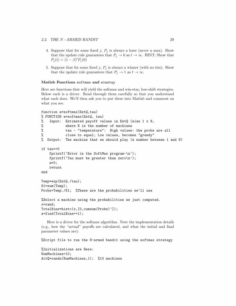
Here are functions that will yield the softmax and win-stay, lose-shift strategies.Below each is a driver. Read through them carefully so that you understandwhat each does. We’ll then ask you to put these into Matlab and comment onwhat you see.

function a=softmax(EstQ,tau)

% FUNCTION a=softmax(EstQ, tau)

% Input: Estimated payoff values in EstQ (size 1 x N,

% where N is the number of machines

% tau - "temperature": High values- the probs are all

% close to equal; Low values, becomes "greedy"

% Output: The machine that we should play (a number between 1 and N)

if tau==0

fprintf(’Error in the SoftMax program-\n’);

fprintf(’Tau must be greater than zero\n’);

a=0;

return

end

Temp=exp(EstQ./tau);

S1=sum(Temp);

Probs=Temp./S1; %These are the probabilities we’ll use

%Select a machine using the probabilities we just computed.

x=rand;

TotalBins=histc(x,[0,cumsum(Probs)’]);

a=find(TotalBins==1);

Here is a driver for the softmax algorithm. Note the implementation details(e.g., how the “actual” payoffs are calculated, and what the initial and finalparameter values are):

%Script file to run the N-armed bandit using the softmax strategy

%Initializations are Here:

NumMachines=10;

ActQ=randn(NumMachines,1); %10 machines


NumPlay=1000; %Play 100 times

Initialtau=10; %Initial tau ("High in beginning")

Endingtau=0.5;

tau=10;

NumPlayed=zeros(NumMachines,1); %Keep a running sum of the number

% of times each action is selected

ValPlayed=zeros(NumMachines,1); %Keep a running sum of the total

% reward for each action

EstQ=zeros(NumMachines,1);

PayoffHistory=zeros(NumPlay,1); %Keep a record of our payoffs

for i=1:NumPlay

%Pick a machine to play:

a=softmax(EstQ,tau);

%Play the machine and update EstQ, tau

Payoff=randn+ActQ(a);

NumPlayed(a)=NumPlayed(a)+1;

ValPlayed(a)=ValPlayed(a)+Payoff;

EstQ(a)=ValPlayed(a)/NumPlayed(a);

PayoffHistory(i)=Payoff;

tau=Initialtau*(Endingtau/Initialtau)^(i/NumPlay);

end

[v,winningmachine]=max(ActQ);

winningmachine

NumPlayed

plot(1:10,ActQ,’k’,1:10,EstQ,’r’)

Here is the function implementing the pursuit strategy (or “Win-Stay, Lose-Shift”).

function [a, P]=winstay(EstQ,P,beta)

% function [a,P]=winstay(EstQ,P,beta)

% Input: EstQ, Estimated values of the payoffs

% P = Probabilities of playing each machine

% beta= parameter to adjust the probabilities, between 0 and 1

% Output: a = Which machine to play

% P = Probabilities for each machine

[vals,idx]=max(EstQ);

winner=idx(1); %Index of our "winning" machine

%Update the probabilities. We need to do P(winner) separately.

NumMachines=length(P);

P(winner)=P(winner)+beta*(1-P(winner));


Temp=1:NumMachines;

Temp(winner)=[]; %Temp now holds the indices of all "losers"

P(Temp)=(1-beta)*P(Temp);

%Probabilities are all updated- Choose machine a w/prob P(a)

x=rand;

TotalBins=histc(x,[0,cumsum(P)’]);

a=find(TotalBins==1);

And its corresponding driver is below. Again, be sure to read and understandwhat each line of the code does:

%Script file to run the N-armed bandit using pursuit strategy

%Initializations

NumMachines=10;

ActQ=randn(NumMachines,1);

NumPlay=2000;

Initialbeta=0.01;

Endingbeta=0.001;

beta=Initialbeta;

NumPlayed=zeros(NumMachines,1);

ValPlayed=zeros(NumMachines,1);

EstQ=zeros(NumMachines,1);

Probs=(1/NumMachines)*ones(10,1);

for i=1:NumPlay

%Pick a machine to play:

[a,Probs]=winstay(EstQ,Probs,beta);

%Play the machine and update EstQ, tau

Payoff=randn+ActQ(a);

NumPlayed(a)=NumPlayed(a)+1;

ValPlayed(a)=ValPlayed(a)+Payoff;

EstQ(a)=ValPlayed(a)/NumPlayed(a);

beta=Initialbeta*(Endingbeta/Initialbeta)^(i/NumPlay);

end

[v,winningmachine]=max(ActQ);

winningmachine

NumPlayed

plot(1:10,ActQ,’k’,1:10,EstQ,’r’)

Homework: Implement these 4 pieces of code into Matlab, and commenton the performance of each. You might try changing the initial and final values


of the parameters to see if the algorithms are stable to these changes. As youform your comments, recall our two competing goals for these algorithms:

• Estimate the values of the actual payoffs (more accurately, the mean pay-out for each machine).

• Maximize our rewards!

2.2.3 A Summary of Reinforcement Learning

We looked in depth at a basic problem of unsupervised learning- That of tryingto find the best winning slot machine in a bank of many. This problem wasunsupervised because, although we got rewards or punishments by winning orlosing money, we did not know at the beginning of the problem what thosepayoffs would be. That is, there was no expert available to tell us if we weredoing something correctly or not, we had to infer correct behavior from directlyplaying the machines.

We also saw that to solve this problem, we had to do a lot of trial anderror learning- that’s typical in unsupervised learning. Because an expert is notthere to tell us the operating parameters, we have to spend time exploring thepossibilities.

We learned some techniques for translating learning theory into mathemat-ics, and in the process, we learned some commands in Matlab. We don’t expectyou to be an expert programmer - this should be a fairly gentle introduction toprogramming. At this stage, you should be able to read some Matlab code andinterpret the output of an algorithm. Later on, we’ll give you more opportunitiesto produce your own pieces of code.

In summary, we looked at the greedy algorithm, the �−greedy algorithm,the softmax strategy, and the pursuit strategy. You might consider how closely(if at all) these algorithms would reproduce human or animal behavior if giventhe same task.

There are many more topics in Reinforcement Learning to consider, we pre-sented only a short introduction to the topic.

An Introduction to Empirical Modeling - Whitman...

Documents

Transcript of An Introduction to Empirical Modeling - Whitman...