An Introduction to Bayesian Analysis with … SAS400-2014 An Introduction to Bayesian Analysis with...

Paper SAS400-2014

An Introduction to Bayesian Analysis with SAS/STAT® Software

Maura Stokes, Fang Chen, and Funda GunesSAS Institute Inc.

Abstract

The use of Bayesian methods has become increasingly popular in modern statistical analysis, with applica-tions in numerous scientific fields. In recent releases, SAS® has provided a wealth of tools for Bayesiananalysis, with convenient access through several popular procedures as well as the MCMC procedure, whichis designed for general Bayesian modeling. This paper introduces the principles of Bayesian inference andreviews the steps in a Bayesian analysis. It then describes the built-in Bayesian capabilities provided inSAS/STAT®, which became available for all platforms with SAS/STAT 9.3, with examples from the GENMODand PHREG procedures. How to specify prior distributions, evaluate convergence diagnostics, and interpretthe posterior summary statistics is discussed.

Foundations

Bayesian methods have become a staple for the practicing statistician. SAS provides convenient toolsfor applying these methods, including built-in capabilities in the GENMOD, FMM, LIFEREG, and PHREGprocedures (called the built-in Bayesian procedures), and a general Bayesian modeling tool in the MCMCprocedure. In addition, SAS/STAT 13.1 introduced the BCHOICE procedure, which performs Bayesianchoice modeling. With such convenient access, more statisticians are digging in to learn more about thesemethods.

The essence of Bayesian analysis is using probabilities that are conditional on data to express beliefs aboutunknown quantities. The Bayesian approach also incorporates past knowledge into the analysis, and so itcan be viewed as the updating of prior beliefs with current data. Bayesian methods are derived from theapplication of Bayes’ theorem, which was developed by Thomas Bayes in the 1700s as an outgrowth of hisinterest in inverse probabilities.

For events A and B, Bayes’ theorem is expressed as

Pr.AjB/ DPr.BjA/Pr.A/

Pr.B/

It can also be written as

Pr.AjB/ DPr.BjA/Pr.A/

Pr.BjA/Pr.A/C Pr.Bj NA/Pr. NA/

where NA means not A. If you think of A as a parameter � and B as data y, then you have

Pr.� jy/ DPr.yj�/Pr.�/

Pr.y/D

Pr.yj�/Pr.�/Pr.yj�/Pr.�/C Pr.yj N�/Pr. N�/

The quantity Pr.y/ is the marginal probability, and it serves as a normalizing constant to ensure that theprobabilities add up to unity. Because Pr.y/ is a constant, you can ignore it and write

Pr.� jy/ / Pr.yj�/Pr.�/

1

Thus, the likelihood Pr.yj�/ is being updated with the prior Pr.�/ to form the posterior distribution Pr.� jy/.

For a basic example of how you might update a set of beliefs with new data, consider a situation whereresearchers screen for vision problems in children in an after-school program. A study of 14 students chosenat random produces two students with vision issues. The likelihood is obtained from the binomial distribution:

L D

14

2

!p2.1 � p/12

Suppose that the parameter p only takes values { 0.1, 0.12, 0.14, 0.16, 0.18, 0.20}. Researchers haveprior beliefs about the probabilities of these values, and they assign them prior weights. Columns 1 and 2in Table 1 contain the possible values for p and the prior probability weights, respectively. You can thencompute the likelihoods for each of the values for p based on the study results, and then you can weightthem with the corresponding prior weight. Column 5 contains the posterior values, which are the computedvalues displayed in column 4 divided by the normalizing constant 0.2501. Thus, the prior beliefs have beenupdated to a posterior distribution by accounting for the data obtained by the study. The posterior values aresimilar to, but different from, the likelihood.

Table 1 Empirical Posterior Distribution

p Prior Weight Likelihood Prior x Likelihood Posterior0.10 0.10 0.257 0.0257 0.1030.12 0.15 0.2827 0.0424 0.1700.14 0.20 0.2920 0.0584 0.2330.16 0.20 0.2875 0.0576 0.2300.18 0.15 0.2725 0.0410 0.1640.20 0.10 .2501 0.0250 0.100

Total 1 .2501 1

In a nutshell, this is what any Bayesian analysis does: it updates your beliefs about the parameters byaccounting for additional data. You weight the likelihood for the data with the prior distribution to produce theposterior distribution. If you want to estimate a parameter � from data y D fy1; : : : ; yng by using a statisticalmodel described by density p.yj�/, Bayesian philosophy says that you can’t determine � exactly but you candescribe the uncertainty by using probability statements and distributions. You formulate a prior distribution�.�/ to express your beliefs about � . You then update those beliefs by combining the information fromthe prior distribution and the data, described with the statistical model p.� jy/, to generate the posteriordistribution p.� jy/.

p.� jy/ Dp.�;y/p.y/

Dp.yj�/�.�/

p.y/D

p.yj�/�.�/Rp.yj�/�.�/d�

The quantity p.y/ is the normalizing constant of the posterior distribution. It is also called the marginaldistribution, and it is often ignored, as long as it is finite. Hence p.� jy/ is often written as

p.� jy/ / p.yj�/�.�/ D L.�/�.�/

where L is the likelihood and is defined as any function that is proportional to p.yj�/. This expression makesit clear that you are effectively weighting your likelihood with the prior distribution. Depending on the influenceof the prior, your previous beliefs can impact the generated posterior distribution either strongly (subjectiveprior) or minimally (objective or noninformative prior).

Consider the vision example again. Say you want to perform a Bayesian analysis where you assume a flatprior for p, or one that effectively will have no influence. A typical flat prior is the uniform,

�.p/ D 1

2

and because the likelihood for the binomial distribution is written as

L.p/ D

n

y

!py.1 � p/n�y

you can write the posterior distribution as

�.pjy/ / p2.1 � p/12

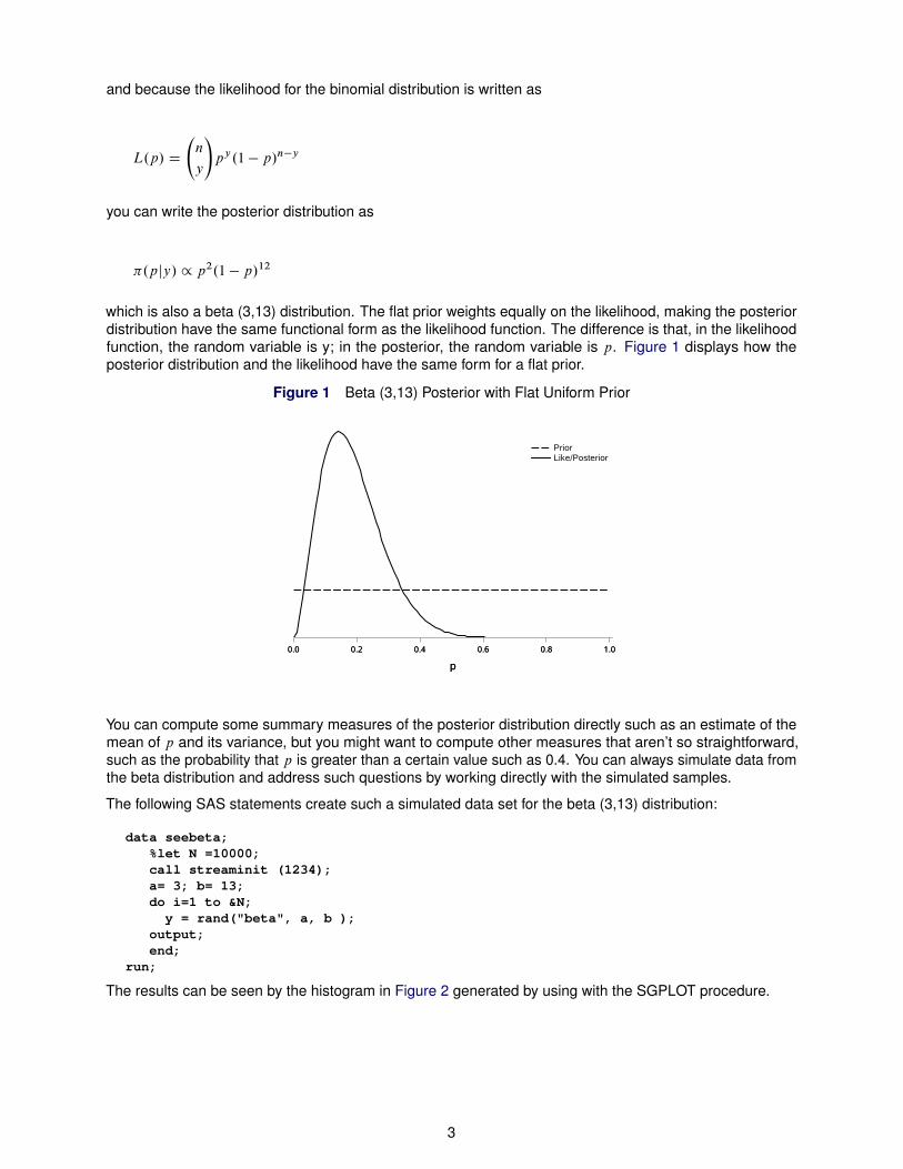
which is also a beta (3,13) distribution. The flat prior weights equally on the likelihood, making the posteriordistribution have the same functional form as the likelihood function. The difference is that, in the likelihoodfunction, the random variable is y; in the posterior, the random variable is p. Figure 1 displays how theposterior distribution and the likelihood have the same form for a flat prior.

Figure 1 Beta (3,13) Posterior with Flat Uniform Prior

0.0 0.2 0.4 0.6 0.8 1.0

p

Like/PosteriorPrior

0.0 0.2 0.4 0.6 0.8 1.0

p

Like/PosteriorPrior

You can compute some summary measures of the posterior distribution directly such as an estimate of themean of p and its variance, but you might want to compute other measures that aren’t so straightforward,such as the probability that p is greater than a certain value such as 0.4. You can always simulate data fromthe beta distribution and address such questions by working directly with the simulated samples.

The following SAS statements create such a simulated data set for the beta (3,13) distribution:

data seebeta;%let N =10000;call streaminit (1234);a= 3; b= 13;do i=1 to &N;y = rand("beta", a, b );

output;end;

run;

The results can be seen by the histogram in Figure 2 generated by using with the SGPLOT procedure.

3

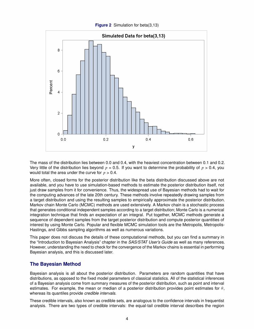
Figure 2 Simulation for beta(3,13)

The mass of the distribution lies between 0.0 and 0.4, with the heaviest concentration between 0.1 and 0.2.Very little of the distribution lies beyond p = 0.5. If you want to determine the probability of p > 0.4, youwould total the area under the curve for p > 0.4.

More often, closed forms for the posterior distribution like the beta distribution discussed above are notavailable, and you have to use simulation-based methods to estimate the posterior distribution itself, notjust draw samples from it for convenience. Thus, the widespread use of Bayesian methods had to wait forthe computing advances of the late 20th century. These methods involve repeatedly drawing samples froma target distribution and using the resulting samples to empirically approximate the posterior distribution.Markov chain Monte Carlo (MCMC) methods are used extensively. A Markov chain is a stochastic processthat generates conditional independent samples according to a target distribution; Monte Carlo is a numericalintegration technique that finds an expectation of an integral. Put together, MCMC methods generate asequence of dependent samples from the target posterior distribution and compute posterior quantities ofinterest by using Monte Carlo. Popular and flexible MCMC simulation tools are the Metropolis, Metropolis-Hastings, and Gibbs sampling algorithms as well as numerous variations.

This paper does not discuss the details of these computational methods, but you can find a summary inthe “Introduction to Bayesian Analysis” chapter in the SAS/STAT User’s Guide as well as many references.However, understanding the need to check for the convergence of the Markov chains is essential in performingBayesian analysis, and this is discussed later.

The Bayesian Method

Bayesian analysis is all about the posterior distribution. Parameters are random quantities that havedistributions, as opposed to the fixed model parameters of classical statistics. All of the statistical inferencesof a Bayesian analysis come from summary measures of the posterior distribution, such as point and intervalestimates. For example, the mean or median of a posterior distribution provides point estimates for � ,whereas its quantiles provide credible intervals.

These credible intervals, also known as credible sets, are analogous to the confidence intervals in frequentistanalysis. There are two types of credible intervals: the equal-tail credible interval describes the region

4

between the cut-points for the equal tails that has 100.1 � ˛/% mass, while the highest posterior density(HPD), is the region where the posterior probability of the region is 100.1 � ˛/% and the minimum densityof any point in that region is equal to or larger than the density of any point outside that region. Somestatisticians prefer the equal-tail interval because it is invariant under transformations. Other statisticiansprefer the HPD interval because it is the smallest interval, and it is more frequently used.

The prior distribution is a mechanism that enables the statistician to incorporate known information into theanalysis and to combine that information with that provided by the observed data. For example, you mighthave expert opinion or historical information from previous studies. You might know the range of values for aparticular parameter for biological reasons. Clearly, the chosen prior distribution can have a tremendousimpact on the results of an analysis, and it must be chosen wisely. The necessity of choosing priors, and itsinherent subjectivity, is the basis for some criticism of Bayesian methods.

The Bayesian approach, with its emphasis on probabilities, does provide a more intuitive framework forexplaining the results of an analysis. For example, you can make direct probability statements aboutparameters, such as that a particular credible interval contains a parameter with measurable probability.Compare this to the confidence interval and its interpretation that, in the long run, a certain percentage ofthe realized confidence intervals will cover the true parameter. Many non-statisticians wrongly assume theBayesian credible interval interpretation for a confidence interval interpretation.

The Bayesian approach also provides a way to build models and perform estimation and inference forcomplicated problems where using frequentist methods is cumbersome and sometimes not obvious. Hierar-chical models and missing data problems are two cases that lend themselves to Bayesian solutions nicely.Although this paper is concerned with less sophisticated analyses in which the driving force is the desire forthe Bayesian framework, it’s important to note that the consummate value of the Bayesian method might beto provide statistical inference for problems that couldn’t be handled without it.

Prior Distributions

Some practitioners want to benefit from the Bayesian framework with as limited an influence from theprior distribution as possible: this can be accomplished by choosing priors that have a minimal impacton the posterior distribution. Such priors are called noninformative priors, and they are popular for someapplications, although they are not always easy to construct. An informative prior dominates the likelihood,and thus it has a discernible impact on the posterior distribution.

A prior distribution is noninformative if it is “flat” relative to the posterior distribution, as demonstrated inFigure 1. However, while a noninformative prior can appear to be more objective, it’s important to realizethat there is some degree of subjectivity in any prior chosen; it does not represent complete ignoranceabout the parameter in question. Also, using noninformative priors can lead to what is known as improperposteriors (nonintegrable posterior density), with which you cannot make inferences. Noninformative priorsmight also be noninvariant, which means that they could be noninformative in one parameterization but notnoninformative if a transformation is applied.

On the other hand, an improper prior distribution, such as the uniform prior distribution on the number line,can be appropriate. Improper prior distributions are frequently used in Bayesian analysis because theyyield noninformative priors and proper posterior distributions. To form a proper posterior distribution, thenormalizing constant has to be finite for all y.

Some of the priors available with the built-in Bayesian procedures are improper, but they all produce properposterior distributions. However, the MCMC procedure enables you to construct whatever prior distributionyou can program, and so you yourself have to ensure that the resulting posterior distribution is proper.

More about Priors

Jeffreys’ prior (Jeffreys 1961) is a useful prior because it doesn’t change much over the region in which thelikelihood is significant and doesn’t have large values outside that range—the local uniformity property. It isbased on the observed Fisher information matrix. Because it is locally uniform, it is a noninformative prior.Thus, it provides an automated way of finding a noninformative prior for any parametric model; it is alsoinvariant with respect to one-to-one transformations. The GENMOD procedure computes Jeffreys’ prior forany generalized linear model, and you can use it for your prior density for any of the coefficient parameters.Jeffreys’ prior can lead to improper posteriors, but not in the case of the PROC GENMOD usage.

5

You can show that Jeffreys’ prior is

�.p/ / p�1=2.1 � p/�1=2

for the binomial distribution, and the posterior distribution for the vision example with Jeffreys’ prior is

L.p/�.p/ / py�12 .1 � p/n�y�

12

� beta.2:5; 12:5/

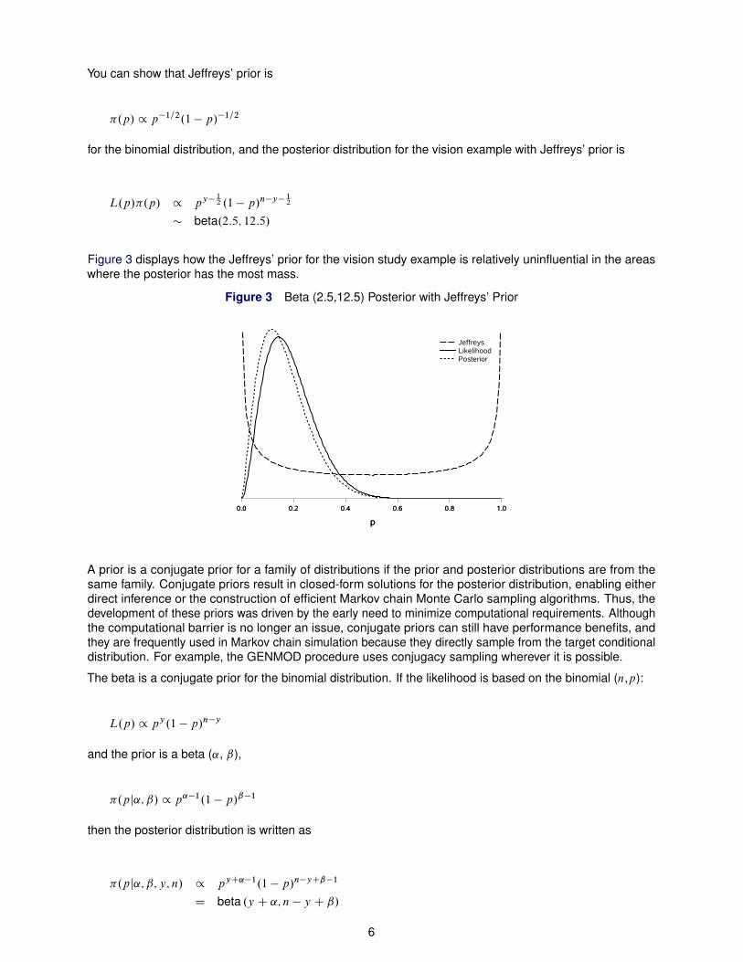
Figure 3 displays how the Jeffreys’ prior for the vision study example is relatively uninfluential in the areaswhere the posterior has the most mass.

Figure 3 Beta (2.5,12.5) Posterior with Jeffreys’ Prior

0.0 0.2 0.4 0.6 0.8 1.0

p

PosteriorLikelihoodJeffreys

0.0 0.2 0.4 0.6 0.8 1.0

p

PosteriorLikelihoodJeffreys

A prior is a conjugate prior for a family of distributions if the prior and posterior distributions are from thesame family. Conjugate priors result in closed-form solutions for the posterior distribution, enabling eitherdirect inference or the construction of efficient Markov chain Monte Carlo sampling algorithms. Thus, thedevelopment of these priors was driven by the early need to minimize computational requirements. Althoughthe computational barrier is no longer an issue, conjugate priors can still have performance benefits, andthey are frequently used in Markov chain simulation because they directly sample from the target conditionaldistribution. For example, the GENMOD procedure uses conjugacy sampling wherever it is possible.

The beta is a conjugate prior for the binomial distribution. If the likelihood is based on the binomial (n,p):

L.p/ / py.1 � p/n�y

and the prior is a beta (˛, ˇ),

�.pj˛; ˇ/ / p˛�1.1 � p/ˇ�1

then the posterior distribution is written as

�.pj˛; ˇ; y; n/ / pyC˛�1.1 � p/n�yCˇ�1

D beta .y C ˛; n � y C ˇ/

6

This posterior is easily calculated, and you can rely on simulations from it to produce the measures ofinterest, as demonstrated above.

Assessing Convergence

Although this paper does not describe the underlying MCMC computations, and you can perform Bayesiananalysis without knowing the specifics of those computations, it is important to understand that a Markovchain is being generated (its stationary distribution is the desired posterior distribution) and that you mustcheck its convergence before you can work with the resulting posterior statistics. An unconverged Markovchain does not explore the parameter space sufficiently, and the samples cannot approximate the targetdistribution well. Inference should not be based on unconverged Markov chains, or misleading results canoccur. And you need to check the convergence of all the parameters, not just the ones of interest.

There is no definitive way of determining that you have convergence, but there are a number of diagnostictools that tell you if the chain hasn’t converged. The built-in Bayesian procedures provide a numberof convergence diagnostic tests and tools, such as Gelman-Rubin, Geweke, Heidelberger-Welch, andRaftery-Lewis tests. Autocorrelation measures the dependency among the Markov chain samples, and highcorrelations can indicate poor mixing. The Geweke statistic compares means from early and late parts of theMarkov chain to see whether they have converged. The effective sample size (ESS) is particularly usefulas it provides a numerical indication of mixing status. The closer ESS is to n, the better the mixing in theMarkov chain. In general, an ESS of approximately 1,000 is adequate for estimating the posterior density.You might want it larger if you are estimating tail percentiles.

One of the ways that you can assess convergence is with visual examination of the trace plot, which is a plotof the sampled values of a parameter versus the sample number. Figure 4 displays some types of traceplots that can result:

Figure 4 Types of Trace Plots

Thinning?

Nonconvergence

Burn-In

Good Mixing

By default, the built-in Bayesian procedures discard the first 2,000 samples as burn-in and keep thenext 10,000. You want to discard the early samples to reduce the potential bias they might have on theestimates.(You can increase the number of samples when needed.) The first plot shows good mixing. Thesamples stay close to the high-density region of the target distribution; they move to the tail areas but

7

quickly return to the high-density region. The second plot shows evidence that a longer burn-in periodis required. The third plot sets off warning signals. You could try increasing the number of samples, butsometimes a chain is simply not going to converge. Additional adjustment might be required such as modelreparameterization or using a different sampling algorithm. Some practitioners might see thinning, or thepractice of keeping every kth iteration to reduce autocorrelation, as indicated. However, current practicetends to downplay the usefulness of thinning in favor of keeping all the samples. The Bayesian proceduresproduce trace plots and also autocorrelation plots and density plots to aid in convergence assessment.

For further information about these measures, see the “Introduction to Bayesian Analysis” chapter in theSAS/STAT User’s Guide.

Summary of the Steps in a Bayesian Analysis

You perform the following steps in a Bayesian analysis. Choosing a prior, checking convergence, andevaluating the sensitivity of your results to your prior might be new steps for many data analysts, but they areimportant ones.

1. Select a model (likelihood) and corresponding priors. If you have information about the parameters,use them to construct the priors.

2. Obtain estimates of the posterior distribution. You might want to start with a short Markov chain.

3. Carry out convergence assessment by using the trace plots and convergence tests. You usually iteratebetween this step and step 2 until you have convergence.

4. Check for the fit of the model and evaluate the sensitivity of your results due to the priors used.

5. Interpret the results: Do the posterior mean estimates make sense? How about the credible intervals?

6. Carry out further analysis: compare different models, or estimate various quantities of interest, such asfunctions of the parameters.

Bayesian Capabilities in SAS/STAT Software

SAS provides two avenues for Bayesian analysis: built-in Bayesian analysis in certain modeling proceduresand the MCMC procedure for general-purpose modeling. The built-in Bayesian procedures are ideal for dataanalysts beginning to use Bayesian methods, and they suffice for many analysis objectives. Simply addingthe BAYES statement generates Bayesian analyses without the need to program priors and likelihoods forthe GENMOD, PHREG, LIFEREG, and FMM procedures. Thus, you can obtain Bayesian results for thefollowing:

• linear regression

• Poisson regression

• logistic regression

• loglinear models

• accelerated failure time models

• Cox proportional models

• piecewise exponential models

• frailty models

• finite mixture models

8

The built-in Bayesian procedures apply the appropriate Markov chain Monte Carlo sampling technique. TheGamerman algorithm is the default sampling method for generalized linear models fit with the GENMODprocedure, and Gibbs sampling with adaptive rejection sampling (ARS) is generally the default, otherwise.However, conjugate sampling is available for a few cases, and the independent Metropolis algorithm and therandom walk Metropolis algorithm are also available when appropriate.

The built-in Bayesian procedures provide default prior distributions depending on what models are specified.You can choose from other available priors by using the CPRIOR= option (for coefficient parameters) andSCALEPRIOR= option (for scale parameters). Other options allow you to choose the numbers of burn-ins,the number of iterations, and so on. The following posterior statistics are produced:

• point estimates: mean, standard deviation, percentiles

• interval estimates: equal-tail and highest posterior density (HPD) intervals

• posterior correlation matrix

• deviance information criteria (DIC)

All these procedures produce convergence diagnostic plots and statistics, and they are the same diagnosticsthat the MCMC procedure produces. You can also output posterior samples to a data set for further analysis.The following sections describe how to use the built-in Bayesian procedures to perform Bayesian analyses.

Linear Regression

Consider a study of 54 patients who undergo a certain type of liver operation in a surgical unit (Neter el al1996). Researchers are interested in whether blood clotting score has a positive effect on survival.

The following statements create SAS data set SURGERY. The variable Y is the survival time, and LOGX1 isthe natural logarithm of the blood clotting score.

data surgery;input x1 logy;y = 10**logy;label x1 = 'Blood Clotting Score';label y = 'Survival Time';logx1 = log(x1);

datalines;6.7 2.30105.1 2.0043....;run;

Suppose you want to perform a Bayesian analysis for the following regression model for the survival times,where � is a N.0; �2/ error term:

Y D ˇ0 C ˇ1logX1 C �

If you wanted a frequentist analysis, you could fit this model by using the REG procedure. But this model isalso a generalized linear model (GLM) with a normal distribution and the identity link function, so it can be fitwith the GENMOD procedure, which offers Bayesian analysis. To review, a GLM relates a mean response toa vector of explanatory variables through a monotone link function where the likelihood function belongsto the exponential family. The link function g describes how the expected value of the response variable isrelated to the linear predictor,

g.E.yi // D g.�i / D xtiˇ

9

where yi is a response variable .i D 1; : : : ; n/, g is a link function, �i D E.yi /, xi is a vector of independentvariables, and ˇ is a vector of regression coefficients to be estimated. For example, when you assume anormal distribution for the response variable, you specify an identity link function g.�/ D �. For Poissonregression you specify a log link function g.�/ D log.�/, and for a logistic regression you specify a logit linkfunction g.�/ D log

��1��

�.

The BAYES statement produces Bayesian analyses with the GENMOD procedure for most of the models itfits; currently this does not include models for which the multinomial distribution is used. The first step of aBayesian analysis is specifying the prior distribution, and Table 2 describes priors that are supported by theGENMOD procedure.

Table 2 Prior Distributions Provided by the GENMOD Procedure

Parameter Prior

Regression coefficients Jeffreys’, normal, uniformDispersion Gamma, inverse gamma,

improperScale and precision Gamma, improper

You would specify a prior for one of the dispersion, scale, or precision parameters, in models that have suchparameters.

The following statements request a Bayesian analysis for the linear regression model with PROC GENMOD:

proc genmod data=surg;model y=logx1/dist=normal;bayes seed=1234 outpost=Post;

run;

The MODEL statement with the DIST=NORMAL option describes the simple linear regression model (thedefault is the identity link function.) The BAYES statement requests the Bayesian analysis. The SEED=option in the BAYES statement sets the random number seed so you can reproduce the analysis in the future.The OUTPOST= option saves the generated posterior samples to the POST data set for further analysis.

By default, PROC GENMOD produces the maximum likelihood estimates of the model parameters, asdisplayed in Figure 5.

Figure 5 Maximum Likelihood Parameter Estimates

Analysis Of Maximum Likelihood Parameter Estimates

Parameter DF EstimateStandard

ErrorWald 95%

Confidence Limits

Intercept 1 -94.9822 114.5279 -319.453 129.4884

logx1 1 170.1749 65.8373 41.1361 299.2137

Scale 1 135.7963 13.0670 112.4556 163.9815

Note: The scale parameter was estimated by maximumlikelihood.

Subsequent tables are produced by the Bayesian analysis. The “Model Information” table in Figure 6summarizes information about the model that you fit. The 2,000 burn-in samples are followed by 10,000samples. Because the normal distribution was specified in the MODEL statement, PROC GENMOD exploitedthe conjugacy and sampled directly from the target distribution.

10

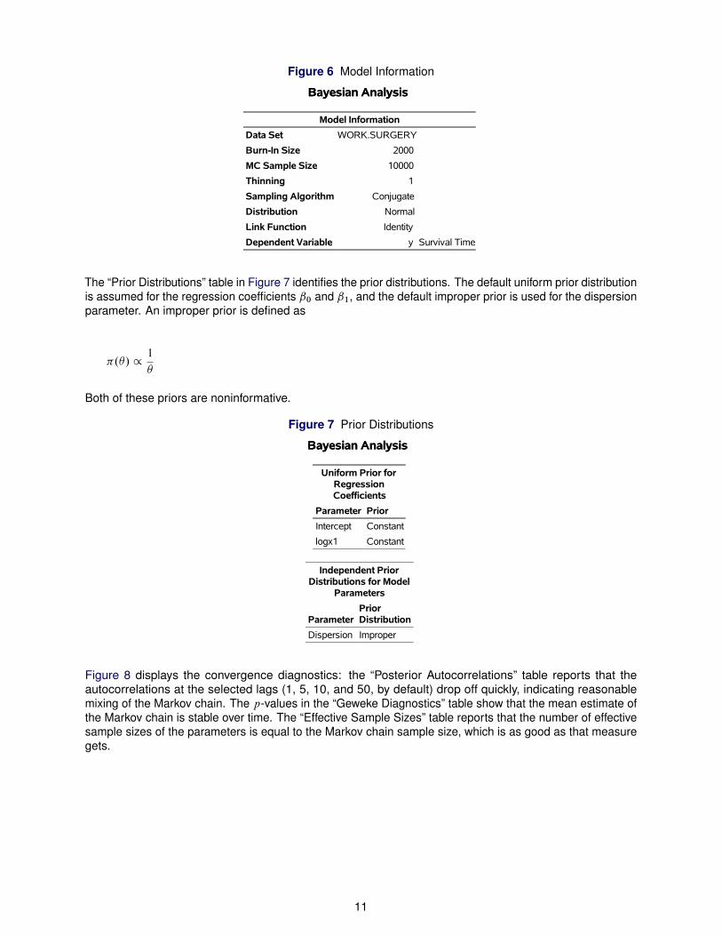
Figure 6 Model Information

Bayesian AnalysisBayesian Analysis

Model Information

Data Set WORK.SURGERY

Burn-In Size 2000

MC Sample Size 10000

Thinning 1

Sampling Algorithm Conjugate

Distribution Normal

Link Function Identity

Dependent Variable y Survival Time

The “Prior Distributions” table in Figure 7 identifies the prior distributions. The default uniform prior distributionis assumed for the regression coefficients ˇ0 and ˇ1, and the default improper prior is used for the dispersionparameter. An improper prior is defined as

�.�/ /1

�

Both of these priors are noninformative.

Figure 7 Prior Distributions


Uniform Prior forRegressionCoefficients

Parameter Prior

Intercept Constant

logx1 Constant

Independent PriorDistributions for Model

Parameters

ParameterPriorDistribution

Dispersion Improper

Figure 8 displays the convergence diagnostics: the “Posterior Autocorrelations” table reports that theautocorrelations at the selected lags (1, 5, 10, and 50, by default) drop off quickly, indicating reasonablemixing of the Markov chain. The p-values in the “Geweke Diagnostics” table show that the mean estimate ofthe Markov chain is stable over time. The “Effective Sample Sizes” table reports that the number of effectivesample sizes of the parameters is equal to the Markov chain sample size, which is as good as that measuregets.

11

Figure 8 Convergence Diagnostics Table


Posterior Autocorrelations

Parameter Lag 1 Lag 5 Lag 10 Lag 50

Intercept 0.0059 0.0145 -0.0059 0.0106

logx1 0.0027 0.0124 -0.0046 0.0091

Dispersion 0.0002 -0.0031 0.0074 0.0014

Geweke Diagnostics

Parameter z Pr > |z|

Intercept -0.2959 0.7673

logx1 0.2873 0.7739

Dispersion 0.9446 0.3449

Effective Sample Sizes

Parameter ESSAutocorrelation

Time Efficiency

Intercept 10000.0 1.0000 1.0000

logx1 10000.0 1.0000 1.0000

Dispersion 10000.0 1.0000 1.0000

The built-in Bayesian procedures produce three types of plots that help you visualize the posterior samplesof each parameter. These diagnostics plots for the slope coefficient ˇ1 are shown in Figure 9. The traceplot indicates that the Markov chain has stabilized with good mixing. The autocorrelation plot confirms thetabular information, and the kernel density plot estimates the posterior marginal distribution. The diagnosticplots for the other parameters (not shown here) have similar outcomes.

Figure 9 Bayesian Model Diagnostic Plot for ˇ1

12

Because convergence doesn’t seem to be an issue, you can review the posterior statistics displayed inFigure 10 and Figure 11.

Figure 10 Posterior Summary Statistics


Posterior Summaries

Percentiles

Parameter N MeanStandardDeviation 25% 50% 75%

Intercept 10000 -95.9018 119.4 -176.1 -96.0173 -16.2076

logx1 10000 170.7 68.6094 124.2 171.1 216.7

Dispersion 10000 19919.9 4072.4 17006.0 19421.7 22253.7

Figure 11 Posterior Interval Statistics

Posterior Intervals

Parameter AlphaEqual-Tail

Interval HPD Interval

Intercept 0.050 -328.7 135.5 -324.0 139.2

logx1 0.050 37.4137 304.3 36.8799 303.0

Dispersion 0.050 13475.4 29325.9 12598.8 28090.3

The posterior summaries displayed in Figure 10 are similar to the maximum likelihood estimates shown inFigure 5. This is because noninformative priors were used and the posterior is effectively the likelihood.Figure 11 displays the HPD interval and the equal-tail interval.

You might be interested in whether LOGX1 has a positive effect on survival time. You can address thisquestion by using the posterior samples that are saved to the POST data set. This means that you candetermine the conditional probability Pr.ˇ1 > 0 j y/ directly from the posterior sample. All you have to do isto determine the proportions of samples where ˇ1 > 0,

Pr.ˇ1 > 0 j y/ D1

N

NXtD1

I.ˇt1 > 0/

where N = 10000 is the number of samples after burn-in and I is an indicator function, where I.ˇt1 > 0/ D 1if ˇt1 > 0, and 0 otherwise. The following SAS statements produce the posterior samples of the indicatorfunction I by using the posterior samples of ˇ1 saved in the output data set POST:

data Prob;set Post;Indicator = (logX1 > 0);label Indicator= 'log(Blood Clotting Score) > 0';

run;

The following statements request the summary statistics by using the MEANS procedure:

proc means data = prob(keep=Indicator);run;

Figure 12 displays the results. The posterior probability that ˇ1 greater than 0 is estimated as 0.9936.Obviously LOGX1 has a strongly positive effect on survival time.

13

Figure 12 Posterior Summary Statistics with the MEANS Procedure

Analysis Variable : Indicator log(Blood ClottingScore) > 0

N Mean Std Dev Minimum Maximum

10000 0.9936000 0.0797476 0 1.0000000

Logistic Regression

Consider a study of the analgesic effects of treatments on elderly patients with neuralgia. A test treatmentand a placebo are compared, and the response is whether the patient reports pain. Explanatory variablesinclude the age and gender of the 60 patients and the duration of the complaint before the treatment began.

The following SAS statements input the data:

data Neuralgia;input Treatment $ Sex $ Age Duration Pain $ @@;

datalines;P F 68 1 No B M 74 16 No P F 67 30 NoP M 66 26 Yes B F 67 28 No B F 77 16 NoA F 71 12 No B F 72 50 No B F 76 9 YesA M 71 17 Yes A F 63 27 No A F 69 18 Yes....;

Logistic regression is considered for this data set:

paini � binary.pi /pi D logit.ˇ0 C ˇ1 � SexF;i C ˇ2 � TreatmentA;i

Cˇ3 � TreatmentB;i C ˇ4 � SexF;i � TreatmentA;iCˇ5 � SexF;i � TreatmentB;i C ˇ6 � AgeC ˇ7 � Duration/

where SexF , TreatmentA, and TreatmentB are dummy variables for the categorical predictors.

You might consider a normal prior with large variance as a noninformative prior distribution on all theregression coefficients:

�.ˇ0; � � � ; ˇ7/ � normal.0; var D 1e6/

You can also fit this model with the GENMOD procedure. The following statements specify the analysis:

proc genmod data=neuralgia;class Treatment(ref="P") Sex(ref="M");model Pain= sex|treatment Age Duration / dist=bin link=logit;bayes seed=1 cprior=normal(var=1e6) outpost=neuout plots=trace nmc=20000;

run;

The CPRIOR=NORMAL(VAR=1E6) option specifies the normal prior for the coefficients; the specified largevariance is requested with VAR=1E6. The PLOTS=TRACE option requests only the trace plots. Logisticregression is requested with the DIST=BIN and the LINK=LOGIT options (either one will do). The defaultsampling algorithm for generalized linear models is the Gamerman algorithm, which uses an iterativeweighted least squares algorithm to sample the coefficients from their conditional distributions. It usuallyperforms very well. The NMC option requests 20,000 samples and is specified because the default numberof simulations results in low ESS.

Figure 13 displays the trace plots for some of the parameters. They show good mixing.

14

Figure 13 Trace Plots

The effective sample sizes are adequate and do not indicate any issues in the convergence of the Markovchain, as seen in Figure 14. With 20,000 samples, the chain has stabilized appropriately.

Figure 14 Effective Sample Sizes

Effective Sample Sizes

Parameter ESSAutocorrelation

Time Efficiency

Intercept 685.2 29.1890 0.0343

SexF 569.3 35.1325 0.0285

TreatmentA 401.8 49.7762 0.0201

TreatmentB 491.7 40.6781 0.0246

TreatmentASexF 596.4 33.5373 0.0298

TreatmentBSexF 585.2 34.1753 0.0293

Age 604.3 33.0943 0.0302

Duration 1054.7 18.9619 0.0527

Thus, the posterior summaries are of interest. Figure 15 displays the posterior summaries and Figure 16displays the posterior intervals.

15

Figure 15 Posterior Summaries


Posterior Summaries

Percentiles

Parameter N MeanStandardDeviation 25% 50% 75%

Intercept 20000 19.6387 7.5273 14.2585 19.6414 24.4465

SexF 20000 2.7964 1.6907 1.6403 2.6644 3.7348

TreatmentA 20000 4.5857 1.9187 3.3402 4.4201 5.5466

TreatmentB 20000 5.0661 1.9526 3.7114 4.8921 6.2388

TreatmentASexF 20000 -1.0052 2.3403 -2.3789 -0.9513 0.5297

TreatmentBSexF 20000 -0.2559 2.2854 -1.7394 -0.2499 1.2874

Age 20000 -0.3365 0.1134 -0.4192 -0.3316 -0.2522

Duration 20000 0.00790 0.0375 -0.0164 0.00668 0.0312

Figure 16 Posterior Intervals

Posterior Intervals

Parameter AlphaEqual-Tail

Interval HPD Interval

Intercept 0.050 5.7037 35.4140 4.0078 32.9882

SexF 0.050 -0.0605 6.5737 0.0594 6.6094

TreatmentA 0.050 1.3776 9.4931 1.2502 8.9476

TreatmentB 0.050 1.6392 9.2298 1.7984 9.3168

TreatmentASexF 0.050 -5.8694 3.4826 -5.9435 3.2389

TreatmentBSexF 0.050 -4.7975 4.3188 -4.1485 4.4298

Age 0.050 -0.5721 -0.1338 -0.5422 -0.1159

Duration 0.050 -0.0637 0.0869 -0.0669 0.0821

The intervals suggest that treatment is highly influential, and although age appears to be important, othercovariates and the sex � treatment interactions do not appear to be important. However, all terms are keptin the model.

Odds ratios are an important measure of association that can be estimated by forming functions of theparameter estimates for a logistic regression. See Stokes, Davis, and Koch (2012) for a full discussion. Forexample, if you want to form an odds ratio comparing the odds of no pain for the female patients to the oddsof no pain for the male patients, you can compute it by exponentiating the corresponding linear combinationof the relevant model parameters.

Because a function of random variables is also a random variable, you can compute odds ratios from theresults of a Bayesian analysis by manipulating the posterior samples. You save the results of your analysis toa special data set known as a SAS item store using the STORE statement, and then you compute the oddsratio by using the ESTIMATE statement of the PLM procedure. PROC PLM performs postfitting tasks byoperating on the posterior samples from PROC GENMOD. (For an MLE analysis, it operates on the savedparameter estimates and covariances.) Recall that the ESTIMATE statement provides custom hypotheses,which means that it can also be used to form functions from the linear combinations of the regressioncoefficients.

The following statements fit the same model with PROC GENMOD and saves the posterior samples to theLOGIT_BAYES item store:

proc genmod data=neuralgia;class Treatment(ref="P") Sex(ref="M");model Pain= sex|treatment Age Duration / dist=bin link=logit;bayes seed=2 cprior=normal(var=1e6) outpost=neuout

16

plots=trace algorithm=im;store logit_bayes;

run;

Note that a different sampler is requested with the SAMPLING=IM option, which requests the IndependenceMetropolis sampler, which is a variation of the Metropolis sampling algorithm. This sampler finds an envelopedistribution to the posterior and uses it as an efficient proposal distribution to generate the posterior samples.It is generally faster than the Gamerman algorithm, but the latter is more computationally stable so it remainsthe default sampler in PROC GENMOD. In this case, the IM sampler produces better ESS values.

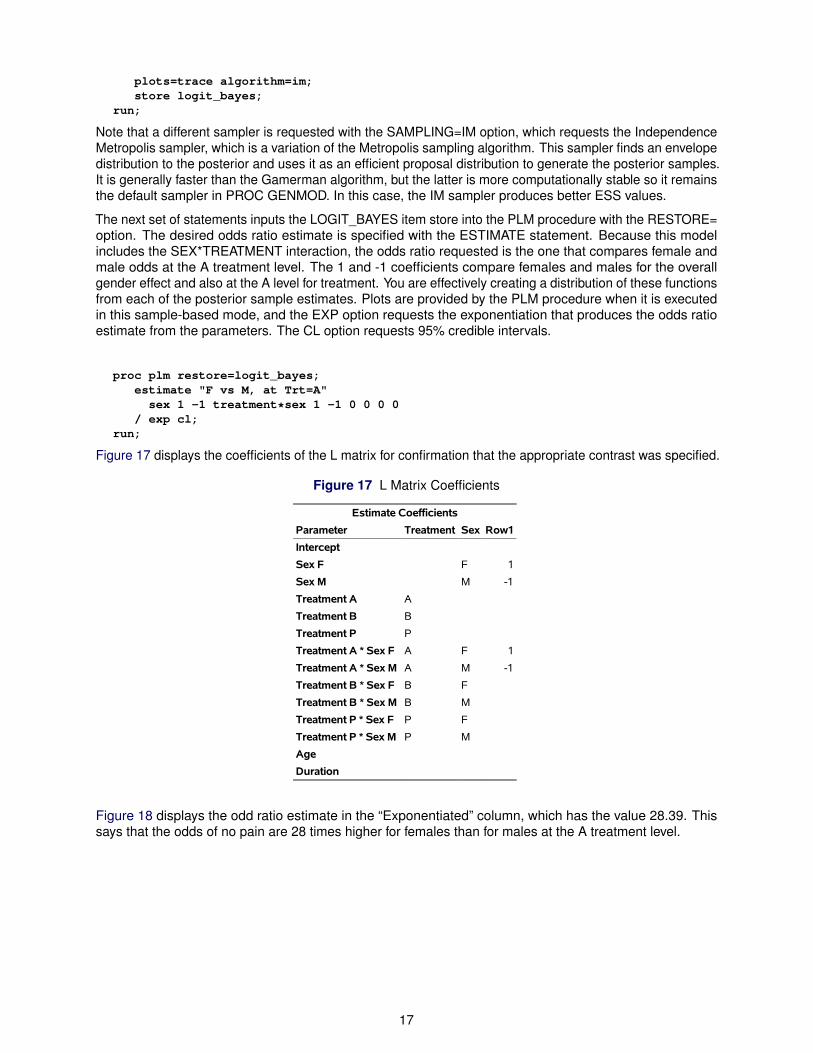
The next set of statements inputs the LOGIT_BAYES item store into the PLM procedure with the RESTORE=option. The desired odds ratio estimate is specified with the ESTIMATE statement. Because this modelincludes the SEX*TREATMENT interaction, the odds ratio requested is the one that compares female andmale odds at the A treatment level. The 1 and -1 coefficients compare females and males for the overallgender effect and also at the A level for treatment. You are effectively creating a distribution of these functionsfrom each of the posterior sample estimates. Plots are provided by the PLM procedure when it is executedin this sample-based mode, and the EXP option requests the exponentiation that produces the odds ratioestimate from the parameters. The CL option requests 95% credible intervals.

proc plm restore=logit_bayes;estimate "F vs M, at Trt=A"sex 1 -1 treatment*sex 1 -1 0 0 0 0

/ exp cl;run;

Figure 17 displays the coefficients of the L matrix for confirmation that the appropriate contrast was specified.

Figure 17 L Matrix Coefficients

Estimate Coefficients

Parameter Treatment Sex Row1

Intercept

Sex F F 1

Sex M M -1

Treatment A A

Treatment B B

Treatment P P

Treatment A * Sex F A F 1

Treatment A * Sex M A M -1

Treatment B * Sex F B F

Treatment B * Sex M B M

Treatment P * Sex F P F

Treatment P * Sex M P M

Age

Duration

Figure 18 displays the odd ratio estimate in the “Exponentiated” column, which has the value 28.39. Thissays that the odds of no pain are 28 times higher for females than for males at the A treatment level.

17

Figure 18 Posterior Odds Ratio Estimate

Sample Estimate

Percentiles

Label N EstimateStandardDeviation 25th 50th 75th Alpha

LowerHPD

UpperHPD Exponentiated

StandardDeviation of

Exponentiated

F vs M, at Trt=A 10000 1.8781 1.5260 0.7768 1.7862 2.9174 0.05 -0.7442 4.9791 28.3873 188.824003

Sample Estimate

Percentiles forExponentiated

Label 25th 50th 75thLower HPD ofExponentiated

Upper HPD ofExponentiated

F vs M, at Trt=A 2.1744 5.9664 18.4925 0.1876 93.1034

Proportional Hazards Model

Consider the data from the Veteran Adminstration’s lung cancer trial that are presented in Appendix 1 ofKalbfleisch and Prentice (1980). Death in days is the response, and type of therapy, type of tumor cell,presence of prior therapy, age, and time from diagnosis to study inclusion are included in the data set. Thereis also an indicator variable for whether the response was censored.

The first 20 observations of SAS data set VALUNG are shown in Figure 19.

below:

Figure 19 Subset of VALUNG Data

Obs Therapy Cell Time Kps Duration Age Ptherapy Status

1 standard squamous 72 60 7 69 no 1

2 standard squamous 411 70 5 64 yes 1














16 standard small 30 60 3 61 no 1



19 standard small 54 80 4 63 yes 1


Interest lies in how therapy and the other covariates impact time until death, and the analysis is furthercomplicated because the response is censored. The proportional hazards model, or Cox regression model,is widely used in the analysis of time-to-event data to explain the effect of explanatory variables on hazardrates. The survival time of each member of a population is assumed to follow its own hazard function �i .t/,

18

�l .t/ D �.t IZl / D �0.t/ exp.Z0lˇ/

where �0.t/ is an arbitrary and unspecified baseline hazard function, Zl is the vector of explanatory variablesfor the l th individual, and ˇ is the vector of unknown regression parameters (which is assumed to be thesame for all individuals). The PHREG procedure fits the Cox model by maximizing the partial likelihoodfunction; this eliminates the unknown baseline hazard �0.t/ and accounts for censored survival times. Inthe Bayesian approach, the partial likelihood function is used as the likelihood function in the posteriordistribution (Sinha, Ibrahim, and Chen 2003).

The PHREG procedure supports the following priors for proportional hazards regression, displayed in Table3.

Table 3 Prior Distributions for the Cox ModelParameter Prior

Regression coefficients Normal, uniform, Zellner’s g-priorZellner’s g Constant, gamma

The following PROC PHREG statements request Bayesian analysis for the Cox proportional hazard modelwith uniform priors on the regression coefficients. The categorical variables PTHERAPY, CELL, andTHERAPY are declared in the CLASS statement. The value “large” is specified as the reference category fortype of tumor cell, the value “standard” is specified as the reference category for therapy, and the value “no”is the reference category for prior therapy.

proc phreg data=VALung;class Ptherapy(ref='no') Cell(ref='large') Therapy(ref='standard');model Time*Status(0) = Kps Duration Age Ptherapy Cell Therapy;hazardratio 'HR' Therapy;bayes seed=1 outpost=out cprior=uniform plots=density;

run;

The BAYES statement requests Bayesian analysis. The CPRIOR= option specifies the uniform prior for theregression coefficients, and the PLOTS= option requests a panel of posterior density plots for the modelparameters. The HAZARDRATIO statement requests the hazard ratio comparing the odds for therapies.

Figure 20 shows kernel posterior density plots that estimate the posterior marginal distributions for thefirst four regression coefficients. Each plot shows a smooth, unimodal shape for the posterior marginaldistribution.

19

Figure 20 Density Plots

Posterior summary statistics and intervals are shown in Figure 21. Because the prior distribution isnoninformative, the results are similar to those obtained with the standard PROC PHREG analysis (notshown here).

Figure 21 Posterior Summary Statistics


Posterior Summaries and Intervals

Parameter N MeanStandardDeviation

95%HPD Interval

Kps 10000 -0.0327 0.00545 -0.0434 -0.0221

Duration 10000 -0.00170 0.00945 -0.0202 0.0164

Age 10000 -0.00852 0.00935 -0.0270 0.00983

Ptherapyyes 10000 0.0754 0.2345 -0.3715 0.5488

Celladeno 10000 0.7867 0.3080 0.1579 1.3587

Cellsmall 10000 0.4632 0.2731 -0.0530 1.0118

Cellsquamous 10000 -0.4022 0.2843 -0.9550 0.1582

Therapytest 10000 0.2897 0.2091 -0.1144 0.6987

The posterior mean of the hazard ratio in Figure 22 indicates that the standard treatment is more effectivethan the test treatment for individuals who have the given covariates. However, note that both the 95%equal-tailed interval and the 95% HPD interval contain the hazard ratio value of 1, which suggests that thetest therapy is not really different from the standard therapy.

20

Figure 22 Hazard Ratio and Confidence Limits

HR: Hazard Ratios for Therapy

Quantiles

Description N MeanStandardDeviation 25% 50% 75%

95%Equal-Tail

Interval95%

HPD Interval

Therapy standard vs test 10000 0.7651 0.1617 0.6509 0.7483 0.8607 0.4988 1.1265 0.4692 1.0859

Suppose you are interested in estimating the survival curves for two individuals who have similar characteris-tics, one of whom receives the test treatment while the other receives the standard treatment. The followingSAS DATA step creates the PRED data set which includes the covariate values for these individuals:

data Pred;input Ptherapy Kps Duration Age Cell $ Therapy $ @@;format Ptherapy yesno.;datalines;0 58 8.7 60 large standard0 58 8.7 60 large test;

The following statements request the estimation of separate survival curves for these two sets of covariates.The PLOTS= option in the PROC PHREG statement requests survival curves, the OVERLAY suboptionoverlays the curves in the same plot, and the CL= suboption requests the highest posterior density (HPD)confidence limits for the survivor functions. The COVARIATES= option in the BASELINE statement specifiesthe covariates data set PRED.

proc phreg data=VALung plots(overlay cl=hpd)=survival;baseline covariates=Pred;class Therapy(ref='standard') Cell(ref='large') Ptherapy(ref='no');model Time*Status(0) = Kps Duration Age Ptherapy Cell Therapy;bayes seed=1 outpost=out cprior=uniform plots=density;

run;

Figure 23 displays the survival curves for these sets of covariate values along with their HPD confidencelimits.

21

Figure 23 Posterior Survival Curves

Capabilities of SAS Built-In Bayesian Procedures

The examples in this paper provide an introduction to the capabilities of the built-in Bayesian procedures inSAS/STAT. But not only can the GENMOD procedure produce Bayesian analyses for linear regression andlogistic regression, it also provides Bayesian analysis for Poisson regression, negative binomial regression,and models based on the Tweedie distribution. While PROC GENMOD doesn’t offer Bayesian analysisfor zero-inflated models, such as the zero-inflated Poisson model, you can still use the built-in Bayesianprocedures by switching to the FMM procedure, which fits finite mixture models, which includes zero-inflatedmodels.

The FMM procedure provides Bayesian analysis for finite mixtures of normal, T, binomial, binary, Poisson,and exponential distributions. This covers ground from zero-inflated models to clustering for univariate data.PROC FMM applies specialized sampling algorithms, depending on the distribution family and the natureof the model effects, including conjugate samplers and the Metropolis-Hastings algorithm. PROC FMMprovides a single parametric form for the prior but you can adjust it to reflect specific prior information. Itprovides posterior summaries and convergence diagnostics similar to those produced by the other built-inBayesian procedures. See Kessler and McDowell (2012) for an example of Bayesian analysis using theFMM procedure.

This paper illustrates the use of the PHREG procedure to perform Bayesian analysis for Cox regression; itcan handle time-dependent covariates and all TIES= methods. (The Bayesian functionality does not currentlyapply to models that have certain data constraints such as recurrent events.) Bayesian analysis is alsoavailable for the frailty models fit with the PHREG procedure, which enable you to analyze survival times thatare clustered. In addition, PROC PHREG also provides Bayesian analysis for the piecewise exponentialmodel.

The LIFEREG procedure provides Bayesian analysis for parametric lifetime models. This capability is nowavailable for the exponential, 3-parameter gamma, log-logistic, log-normal, logistic, normal, and Weibulldistributions. Model parameters are the regression coefficients and dispersion parameters (or precision orscale). Normal and uniform priors are provided for the regression coefficients, and the gamma and improperpriors are provided for the scale and shape parameters.

22

General Bayesian Modeling with the MCMC Procedure

Although the built-in Bayesian procedures provide Bayesian analyses for many standard techniques, theyonly go so far. You might want to include priors that are not offered, or you might want to perform a Bayesiananalysis for a model that isn’t covered. For example, the GENMOD procedure doesn’t presently offerBayesian analysis for the proportional odds model. However, you can fit nearly any model that you want, forany prior and likelihood you can program, with the MCMC procedure.

The MCMC procedure is a general-purpose Bayesian modeling tool. It was built on the familiar syntax ofprogramming statements used in the NLMIXED procedure. PROC MCMC performs posterior sampling andstatistical inference for Bayesian parametric models. The procedure fits single-level or multilevel models.These models can take various forms, from linear to nonlinear models, by using standard or nonstandarddistributions. Using PROC MCMC requires using programming statement to declare the parameters in themodel, to specify prior distributions for them, and to describe the conditional distribution for the responsevariable given the parameters. You can specify a model by using keywords for a standard form (normal,binomial, gamma) or use programming statements to define a general distribution.

The MCMC procedure uses various algorithms to simulate samples from the model that you specify. You canalso choose an optimization technique (such as the quasi-Newton algorithm) to estimate the posterior modeand approximate the covariance matrix around the mode. PROC MCMC computes a number of posteriorestimates, and it also outputs the posterior samples to a data set for further analysis. The MCMC procedureprovides the same convergence diagnostics that are produced by using a BAYES statement in the built-inBayesian procedures, as discussed previously.

The RANDOM statement in the MCMC procedure facilitates the specification of random effects in hierarchicallinear or nonlinear models. You can build nested or nonnested hierarchical models to arbitrary depth. Usingthe RANDOM statement can result in reduced simulation time and improved convergence for models thathave a large number of subjects. The MCMC procedure also handles missing data for both responsesand covariates. Chen (2009, 2011, 2013) provides good overviews of the capabilities of the MCMCprocedure, which continues to be enhanced. The most recent release of PROC MCMC in SAS/STAT 13.1 ismultithreaded, providing faster performance for many models.

The BCHOICE Procedure

The first SAS/STAT procedure designed to focus on Bayesian analysis for a specific application is theBCHOICE procedure. PROC BCHOICE performs Bayesian analysis for discrete choice models. Discretechoice models are used in marketing research to model decision makers’ choices among alternative productsand services. The decision makers might be people, households, companies, and so on, and the alternativesmight be products, services, actions, or any other options or items about which choices must be made. Thecollection of alternatives is known as a choice set, and when individuals are asked to choose, they usuallyassign a utility to each alternative. The BCHOICE procedure provides Bayesian discrete choice models suchas the multinomial logit, multinomial logit with random effects, and the nested logit. The probit responsefunction is also available. You can supply a prior distribution for the parameters if you want something otherthan the default noninformative prior. PROC BCHOICE obtains samples from the corresponding posteriordistributions, produces summary and diagnostic statistics, and saves the posterior samples to an output dataset that can be used for further analysis. PROC BCHOICE is also multithreaded.

Summary

The SAS built-in Bayesian procedures provide a great deal of coverage for standard statistical analyses. Witha ready set of priors and carefully-chosen default samplers, they make Bayesian computing very convenientfor the SAS/STAT user. They provide a great starting place for the statistician who needs some essentialBayesian analysis now and might want to add more sophisticated Bayesian computing skills later. Bayesiananalysis is an active area in SAS statistical software development, and each new release brings additionalfeatures.

For more information, the “Introduction to Bayesian Analysis” chapter in the SAS/STAT User’s Guide containsa reading list with comprehensive references, including many references at the introductory level. In addition,the Statistics and Operations Focus Area includes substantial information about the statistical products, and

23

you can find it at support.sas.com/statistics/. The quarterly e-newsletter for that site is availableon its home page. And of course, complete information is available in the online documentation locatedat support.sas.com/documentation/onlinedoc/stat/. The features of each new release aredescribed in a “What’s New” chapter that is must reading for SAS/STAT users.

References

Chen, F. (2009), “Bayesian Modeling Using the MCMC Procedure,” in Proceedings of the SAS Global Forum2008 Conference, Cary NC: SAS Institute Inc. Available at http://support.sas.com/resources/papers/proceedings09/257-2009.pdf.

Chen, F. (2011), “The RANDOM Statement and More: Moving on with PROC MCMC,” in Proceedings of theSAS Global Forum 2011 Conference, Cary NC: SAS Institute Inc. Available at http://support.sas.com/resources/papers/proceedings11/334-2011.pdf.

Chen, F. (2013), “Missing No More: Using the MCMC Procedure to Model Missing Data”, in Proceedingsof the SAS Global Forum 2013 Conference, Cary NC: SAS Institute Inc. Available at http://support.sas.com/resources/papers/proceedings11/436-2013.pdf.

Gamerman, D. (1997), “Sampling from the Posterior Distribution in Generalized Linear Mixed Mod-els,”Statistics and Computing, 7, 57–68.

Gilks, W. R. and Wild, P. (1992), “Adaptive Rejection Sampling for Gibbs Sampling,” Applied Statistics, 41,337–348.

Gilks, W. R., Best, N. G., and Tan, K. K. C. (1995), “Adaptive Rejection Metropolis Sampling,” AppliedStatistics, 44, 455–472.

Kalbfleisch, J. D. and Prentice, R. L. (1980), The Statistical Analysis of Failure Time Data, New York: JohnWiley & Sons.

Kessler, D. and McDowell, A. (2012), “Introducing the FMM Procedure for Finite Mixture Models,” inProceedings of the SAS Global Forum 2012 Conference, Cary NC: SAS Institute Inc. Available at http://support.sas.com/resources/papers/proceedings12/328-2012.pdf.

Neter, J., Kutner, M. H., Nachtsheim, C. J., and Wasserman, W. (1996), Applied Linear Statistical Models,Fourth Edition, Chicago: Irwin.

Sinha, D., Ibrahim, J. G., and Chen, M. (2003), “Bayesian Justification of Cox’s Partial Likelihood”, Biometrics,90, 629–641.

Stokes, M. E., Davis, C. E., and Koch G G. (2012). Categorical Data Analysis Using SAS, Third Edition, SASPress: Cary NC.

Acknowledgments

The authors are grateful to Ed Huddleston for editing this manuscript. They would also like to thank DavidKessler and Warren Kuhfeld for their helpful suggestions.

Contact Information

Your comments and questions are valued and encouraged. Contact the author:

Maura StokesSAS Institute Inc.SAS Campus DriveCary, NC 27513

24

support.sas.com/statistics/

support.sas.com/documentation/onlinedoc/stat/

http://support.sas.com/resources/papers/proceedings09/257-2009.pdf








Version

1.0

SAS and all other SAS Institute Inc. product or service names are registered trademarks or trademarks ofSAS Institute Inc. in the USA and other countries. ® indicates USA registration.

Other brand and product names are trademarks of their respective companies.

25

An Introduction to Bayesian Analysis with … SAS400-2014 An Introduction to Bayesian Analysis with...

Documents

Transcript of An Introduction to Bayesian Analysis with … SAS400-2014 An Introduction to Bayesian Analysis with...