An introduc on to Machine Learning
151
An introducWon to Machine Learning Pierre Geurts [email protected] Department of EE and CS & GIGA‐R, BioinformaWcs and modelling University of Liège
Transcript of An introduc on to Machine Learning
An introducWon to Machine Learning
Pierre [email protected]
Department of EE and CS & GIGA‐R, BioinformaWcs and modelling
University of Liège

2
Outline
● IntroducWon
● Supervised Learning
● Other learning protocols/frameworks

3
Machine Learning: definiWon
Machine Learning is concerned with the development, the analysis, and the application of algorithms that allow computers to learn
Learning:
A computer learns if it improves its performance at some task with experience (i.e. by collecWng data)
ExtracWng a model of a system from the sole observaWon (or the simulaWon) of this system in some situaWons.
A model = any relaWonship between the variables used to describe the system.
Two main goals: make predicWon and beXer understand the system

4
Machine learning: when ? Learning is useful when:
Human expertise does not existnavigating on Mars
Humans are unable to explain their expertisespeech recognition
Solution changes in timerouting on a computer network
Solution needs to be adapted to particular casesuser biometrics
Example: It is easier to write a program that learns to play checkers or
backgammon well by self-play rather than converting the expertise of a master player to a program.

5
ApplicaWons: autonomous driving
DARPA Grand challenge 2005: build a robot capable of navigaWng 240 km through desert terrain in less than 10 hours, with no human intervenWon
The actual wining Wme of Stanley [Thrun et al., 05] was 6 hours 54 minutes.
http://www.darpa.mil/grandchallenge/
6
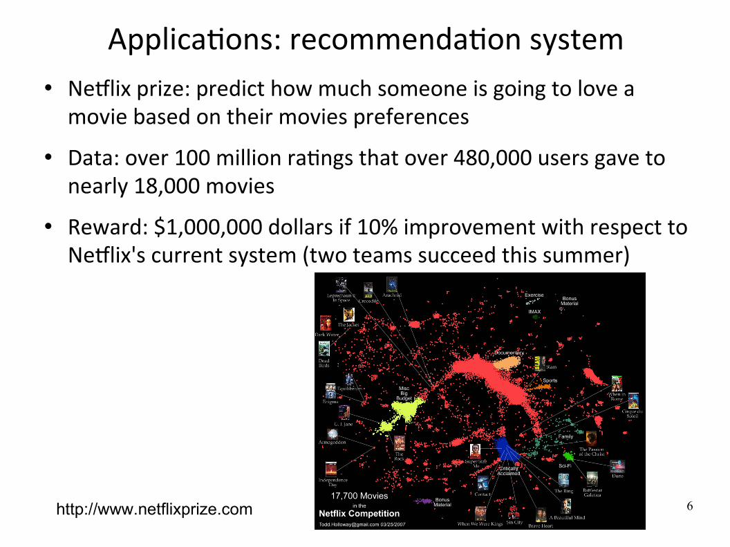
ApplicaWons: recommendaWon system NeVlix prize: predict how much someone is going to love a movie based on their movies preferences
Data: over 100 million raWngs that over 480,000 users gave to nearly 18,000 movies
Reward: $1,000,000 dollars if 10% improvement with respect to NeVlix's current system (two teams succeed this summer)
http://www.netflixprize.com
7
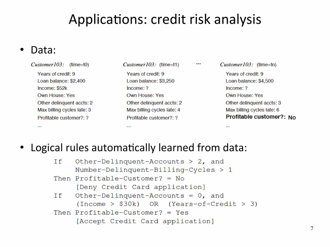
ApplicaWons: credit risk analysis
Data:
Logical rules automaWcally learned from data:

8
Other applicaWons
Machine learning has a wide spectrum of applicaWons including:
Retail: Market basket analysis, Customer relaWonship management (CRM)
Finance: Credit scoring, fraud detecWon Manufacturing: OpWmizaWon, troubleshooWng Medicine: Medical diagnosis TelecommunicaWons: Quality of service opWmizaWon, rouWng BioinformaWcs: MoWfs, alignment Web mining: Search engines ...
9
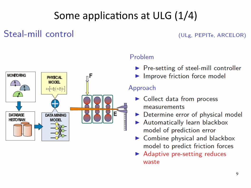
Some applicaWons at ULG (1/4)

10
Some applicaWons at ULG (2/4)

11
Some applicaWons at ULG (3/4)
12
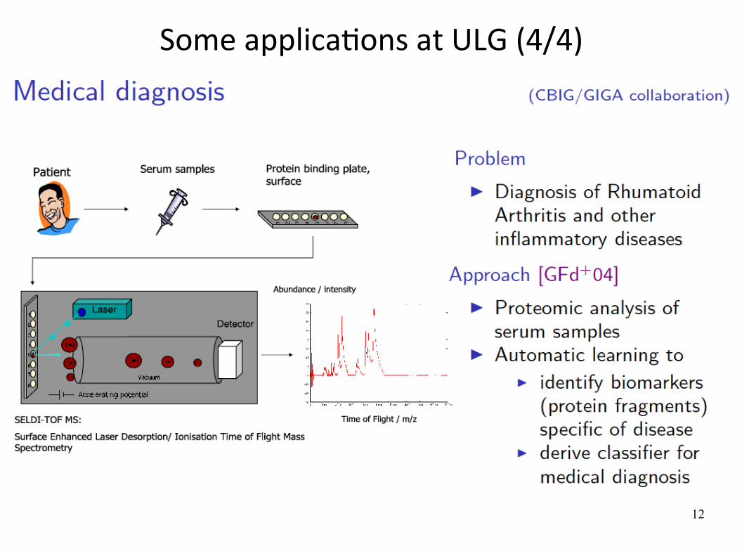
Some applicaWons at ULG (4/4)
13
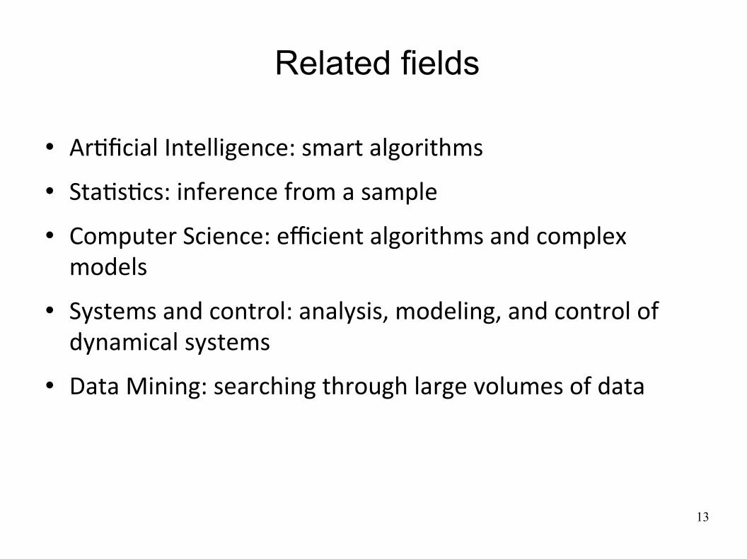
Related fields
ArWficial Intelligence: smart algorithms
StaWsWcs: inference from a sample
Computer Science: efficient algorithms and complex models
Systems and control: analysis, modeling, and control of dynamical systems
Data Mining: searching through large volumes of data
14
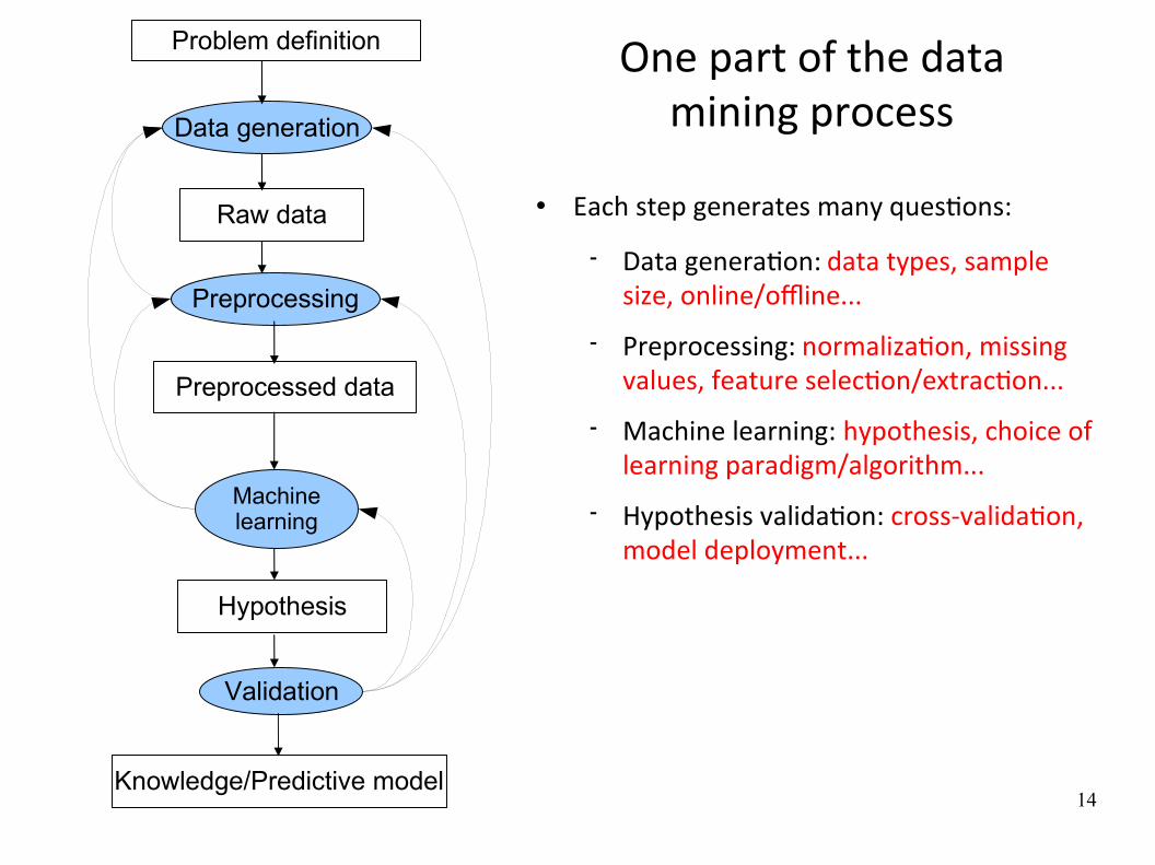
One part of the data mining process
Problem definition
Raw data
Preprocessed data
Preprocessing
Data generation
Machinelearning
Hypothesis
Validation
Knowledge/Predictive model
Each step generates many quesWons:
Data generaWon: data types, sample size, online/offline...
Preprocessing: normalizaWon, missing values, feature selecWon/extracWon...
Machine learning: hypothesis, choice of learning paradigm/algorithm...
Hypothesis validaWon: cross‐validaWon, model deployment...
15
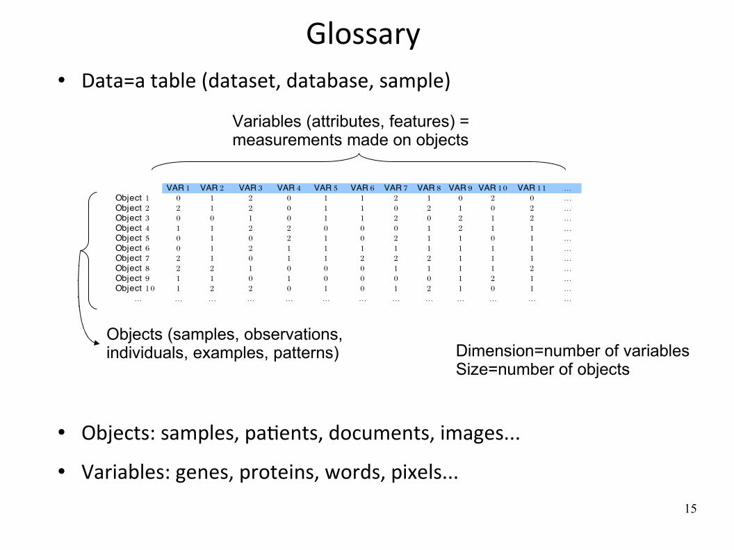
Glossary Data=a table (dataset, database, sample)
Objects: samples, paWents, documents, images...
Variables: genes, proteins, words, pixels...
1VAR 2VAR 3VAR 4VAR 5VAR 6VAR 7VAR 8VAR 9VAR 10VAR 11VAR ... 1Object 0 1 2 0 1 1 2 1 0 2 0 ... 2Object 2 1 2 0 1 1 0 2 1 0 2 ... 3Object 0 0 1 0 1 1 2 0 2 1 2 ... 4Object 1 1 2 2 0 0 0 1 2 1 1 ... 5Object 0 1 0 2 1 0 2 1 1 0 1 ... 6Object 0 1 2 1 1 1 1 1 1 1 1 ... 7Object 2 1 0 1 1 2 2 2 1 1 1 ... 8Object 2 2 1 0 0 0 1 1 1 1 2 ... 9Object 1 1 0 1 0 0 0 0 1 2 1 ... 10Object 1 2 2 0 1 0 1 2 1 0 1 ...
... ... ... ... ... ... ... ... ... ... ... ... ...
Objects (samples, observations, individuals, examples, patterns)
Variables (attributes, features) = measurements made on objects
Dimension=number of variables Size=number of objects

16
Outline
● IntroducWon
● Supervised Learning
IntroducWon Model selecWon, cross‐validaWon, overfiYng Some supervised learning algorithms Beyond classificaWon and regression
● Other learning protocols/frameworks

17
Supervised learning
Goal: from the database (learning sample), find a funcWon f of the inputs that approximates at best the output
Formally:
Symbolic output ⇒ classificaEon, Numerical output ⇒ regression
1X 2X 3X 4X Y-0.61 -0.43 Y 0.51 Healthy-2.3 -1.2 N -0.21 Disease0.33 -0.16 N 0.3 Healthy0.23 -0.87 Y 0.09 Disease-0.69 0.65 N 0.58 Healthy0.61 0.92 Y 0.02 Disease
Supervisedlearning
Inputs Output
Learning samplemodel,hypothesis
18
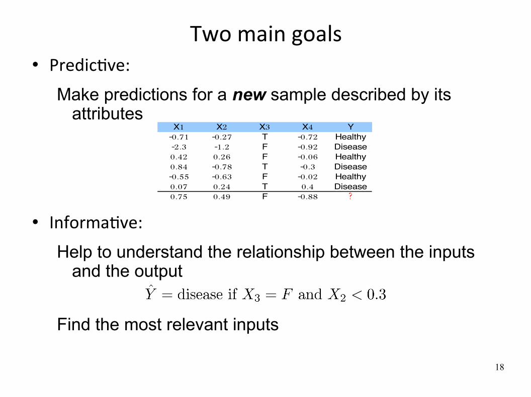
Two main goals PredicWve:
Make predictions for a new sample described by its attributes
InformaWve:
Help to understand the relationship between the inputs and the output
Find the most relevant inputs
1X 2X 3X 4X Y-0.71 -0.27 T -0.72 Healthy-2.3 -1.2 F -0.92 Disease0.42 0.26 F -0.06 Healthy0.84 -0.78 T -0.3 Disease-0.55 -0.63 F -0.02 Healthy0.07 0.24 T 0.4 Disease0.75 0.49 F -0.88 ?

19
Example of applicaWons
Biomedical domain: medical diagnosis, differenWaWon of diseases, predicWon of the response to a treatment...
Patients
Gene expression, Metabolite concentrations...
1X 2X ... 4X Y-0.1 0.02 ... 0.01 Healthy-2.3 -1.2 ... 0.88 Disease0 0.65 ... -0.69 Healthy
0.71 0.85 ... -0.03 Disease-0.18 0.14 ... 0.84 Healthy-0.64 0.15 ... 0.03 Disease
20
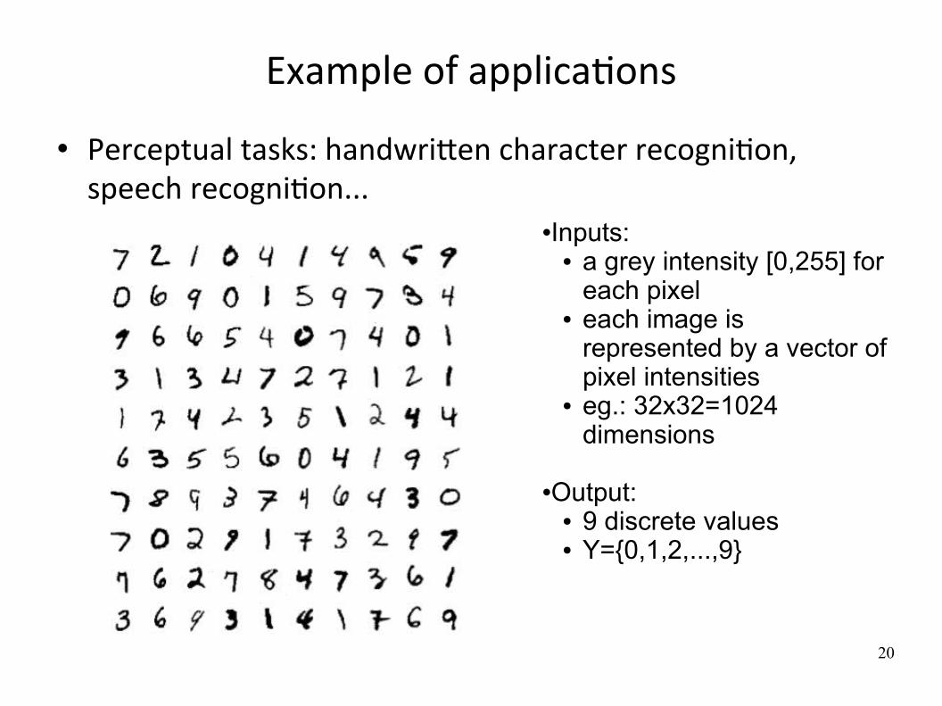
Example of applicaWons
Perceptual tasks: handwriXen character recogniWon, speech recogniWon...
Inputs:● a grey intensity [0,255] for
each pixel● each image is
represented by a vector of pixel intensities
● eg.: 32x32=1024 dimensions
Output:● 9 discrete values● Y={0,1,2,...,9}
21
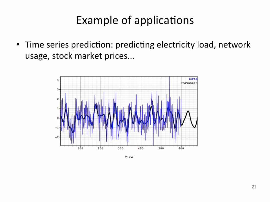
Example of applicaWons
Time series predicWon: predicWng electricity load, network usage, stock market prices...

22
Outline
● IntroducWon
● Supervised Learning
IntroducWon Model selecWon, cross‐validaWon, overfiYng Some supervised learning algorithms Beyond classificaWon and regression
● Other learning protocols/frameworks

23
IllustraWve problem
Medical diagnosis from two measurements (eg., weights and temperature)
Goal: find a model that classifies at best new cases for which X1 and X2 are known
1X 2X Y0.93 0.9 Healthy0.44 0.85 Disease0.53 0.31 Healthy0.19 0.28 Disease... ... ...
0.57 0.09 Disease0.12 0.47 Healthy
0
1
0 1X1
X2
24
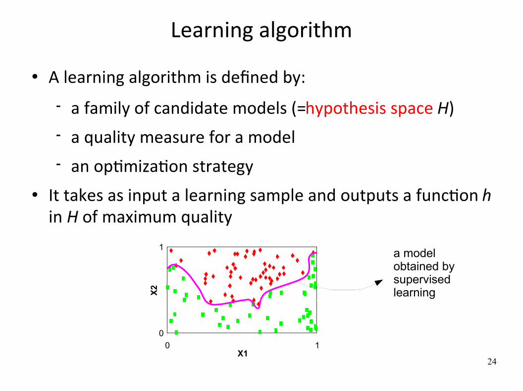
Learning algorithm
A learning algorithm is defined by:
a family of candidate models (=hypothesis space H) a quality measure for a model an opWmizaWon strategy
It takes as input a learning sample and outputs a funcWon h in H of maximum quality
0
1
0 1X1
X2
a model obtained by supervised learning

25
Linear model
Learning phase: from the learning sample, find the best values for w0, w1 and w2
Many alternaWves even for this simple model (LDA, Perceptron, SVM...)
h(X1,X2)=Disease if w0+w1*X1+w2*X2>0Normal otherwise
0
1
0 1X1
X2

26
QuadraWc model
Learning phase: from the learning sample, find the best values for w0, w1,w2, w3 and w4
Many alternaWves even for this simple model (LDA, Perceptron, SVM...)
h(X1,X2)=Disease if w0+w1*X1+w2*X2+w3*X12+w4*X22>0Normal otherwise
0
1
0 1X1
X2
27
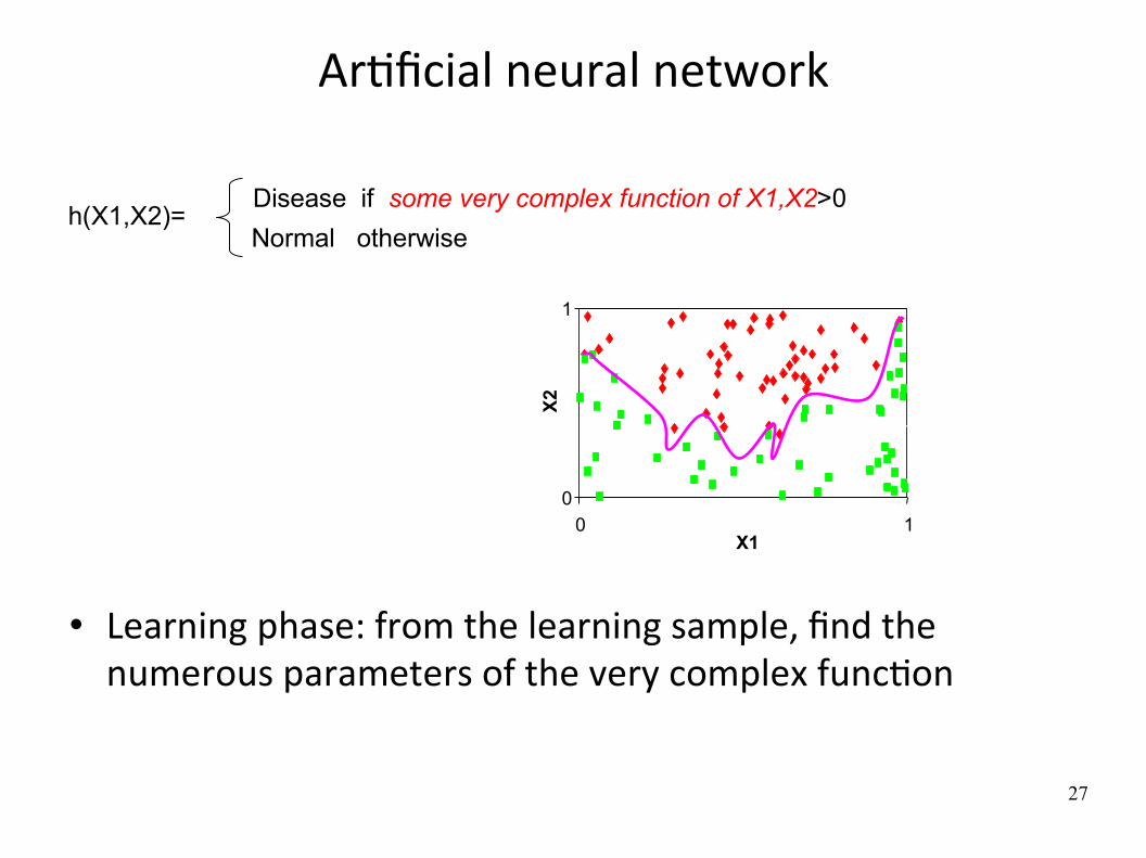
ArWficial neural network
Learning phase: from the learning sample, find the numerous parameters of the very complex funcWon
h(X1,X2)=Disease if some very complex function of X1,X2>0Normal otherwise
0
1
0 1X1
X2

28
Which model is the best?
Why not choose the model that minimises the error rate on the learning sample? (also called re‐subsEtuEon error)
How well are you going to predict future data drawn from the same distribuWon? (generalisaEon error)
0
1
0 10
1
0 10
1
0 1
linear quadratic neural net
29
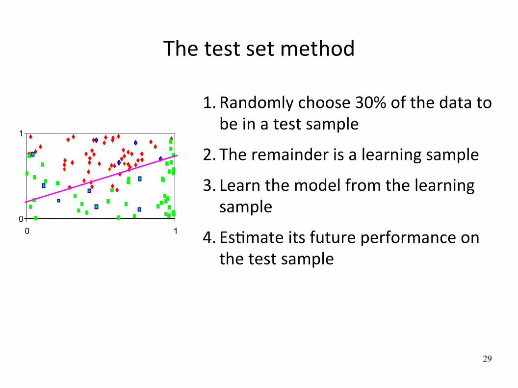
The test set method
1. Randomly choose 30% of the data to be in a test sample
2. The remainder is a learning sample
3. Learn the model from the learning sample
4. EsWmate its future performance on the test sample
0
1
0 1

30
Which model is the best?
We say that the neural network overfits the data
OverfiYng occurs when the learning algorithm starts fiYng noise.
(by opposiWon, the linear model underfits the data)
0
1
0 10
1
0 10
1
0 1
LS error= 3.4%TS error= 3.5%
LS error= 1.0%TS error= 1.5%
LS error= 0%TS error= 3.5%
linear quadratic neural net
31
The test set method
Upside:
very simple ComputaWonally efficient
Downside:
Wastes data: we get an esWmate of the best method to apply to 30% less data
Very unstable when the database is small (the test sample choice might just be lucky or unlucky)

32
Leave‐one‐out Cross ValidaWon
For k=1 to N
remove the kth object from the learning sample
learn the model on the remaining objects
apply the model to get a predicWon for the kth object
report the proporWon of misclassified objects
0
1
0 1
33
Leave‐one‐out Cross ValidaWon
Upside:
Does not waste the data (you get an esWmate of the best method to apply to N‐1 data)
Downside:
Expensive (need to train N models) High variance
34
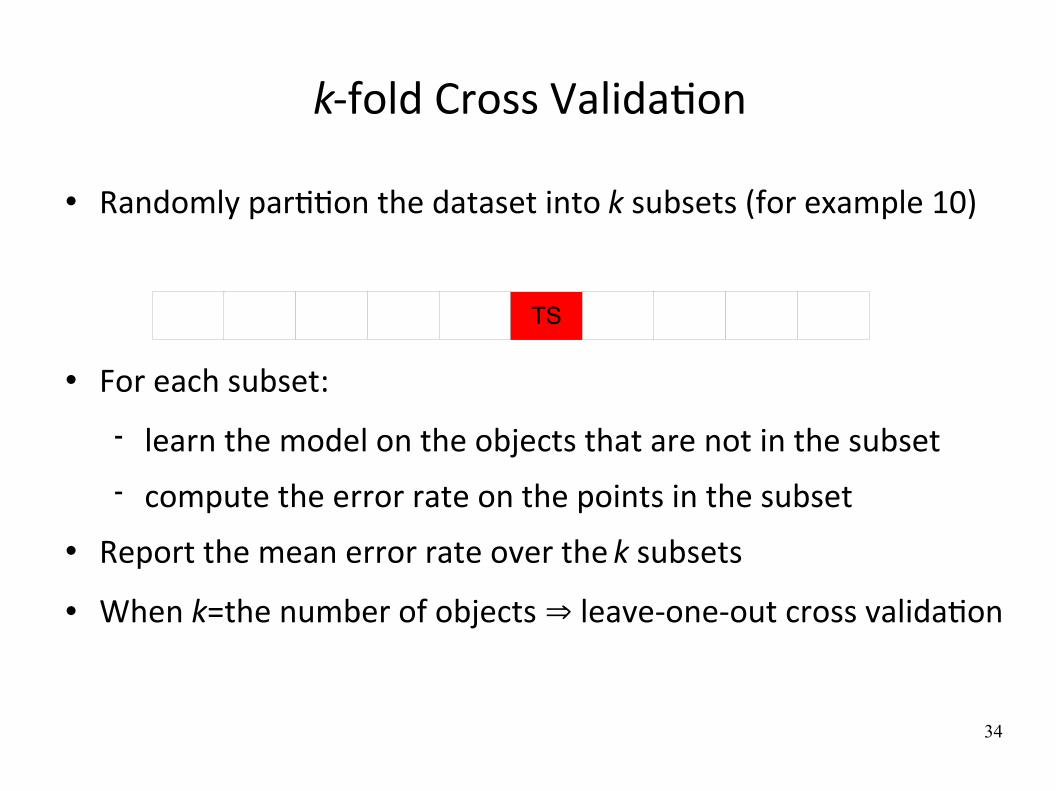
k‐fold Cross ValidaWon
Randomly parWWon the dataset into k subsets (for example 10)
For each subset:
learn the model on the objects that are not in the subset compute the error rate on the points in the subset
Report the mean error rate over the k subsets
When k=the number of objects ⇒ leave‐one‐out cross validaWon
TS

35
Which kind of Cross ValidaWon? Test set:
Cheap but waste data and unreliable when few data
Leave‐one‐out:
Doesn't waste data but expensive
k‐fold cross validaWon:
compromise between the two
Rule of thumb:
a lot of data (>1000): test set validaWon small data (100‐1000): 10‐fold CV very small data(<100): leave‐one‐out CV

36
CV‐based complexity control
Error
Over-fittingUnder-fitting
Optimal complexity Complexity
CV error
LS error

37
Complexity
Controlling complexity is called regularizaWon or smoothing
Complexity can be controlled in several ways
The size of the hypothesis space: number of candidate models, range of the parameters...
The performance criterion: learning set performance versus parameter range, eg. minimizes
Err(LS)+λ C(model) The opWmizaWon algorithms: number of iteraWons, nature of the opWmizaWon problem (one global opWmum versus several local opWma)...

38
CV‐based algorithm choice
Step 1: compute 10‐fold (or test set or LOO) CV error for different algorithms
Step 2: whichever algorithm gave best CV score: learn a new model with all data, and that's the predicWve model
What is the expected error rate of this model?
CV error
Algo 1Algo 2
Algo 3
Algo 4

39
Warning: Intensive use of CV can overfit
If you compare many (complex) models, the probability that you will find a good one by chance on your data increases
SoluWon:
Hold out an addiWonal test set before starWng the analysis (or, beXer, generate this data aFerwards)
Use it to esWmate the performance of your final model
(For small datasets: use two stages of 10‐fold CV)

40
A note on performance measures
Which of these two models is the best?
The choice of an error or quality measure is highly applicaWon dependent.
True class 1Model 2Model1 Negative Posit ive Negat ive2 Negative Negat ive Negat ive3 Negative Posit ive Posit ive4 Negative Posit ive Negat ive5 Negative Negat ive Negat ive6 Negative Negat ive Negat ive7 Negative Negat ive Posit ive8 Negative Negat ive Negat ive9 Negative Negat ive Negat ive
10 Posit ive Posit ive Posit ive11 Posit ive Posit ive Negat ive12 Posit ive Posit ive Posit ive13 Posit ive Posit ive Posit ive14 Posit ive Negat ive Negat ive15 Posit ive Posit ive Negat ive
41
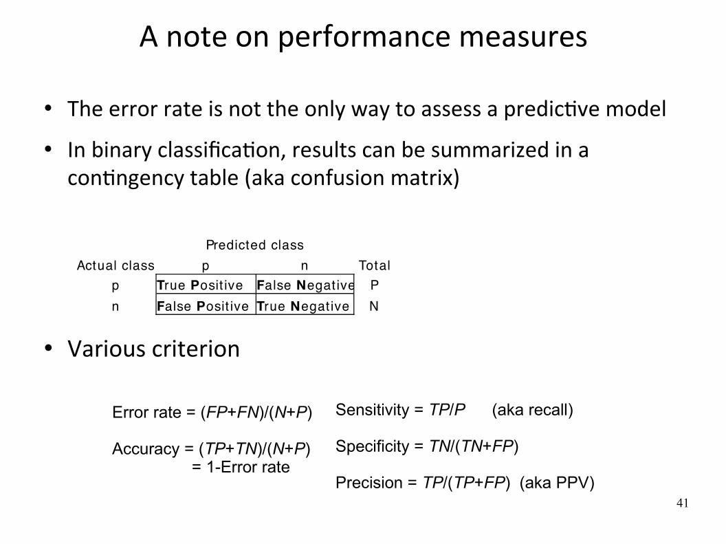
A note on performance measures
The error rate is not the only way to assess a predicWve model
In binary classificaWon, results can be summarized in a conWngency table (aka confusion matrix)
Various criterion
Predicted class Actual class p n Total
p Pn N
T rue Posit ive F alse Negat iveF alse Posit ive T rue Negat ive
Error rate = (FP+FN)/(N+P)
Accuracy = (TP+TN)/(N+P) = 1-Error rate
Sensitivity = TP/P (aka recall)
Specificity = TN/(TN+FP)
Precision = TP/(TP+FP) (aka PPV)

42
ROC and Precision/recall curves Each point corresponds to a parWcular choice of the decision threshold
True
Pos
itive
Rat
e(S
ensi
tivity
)
False Positive Rate(1-Specificity)
Pre
cisi
on
Recall (Sensitivity)

43
Outline IntroducWon
Model selecWon, cross‐validaWon, overfiYng
Some supervised learning algorithms
k‐NN Linear methods ArWficial neural networks Support vector machines Decision trees Ensemble methods
Beyond classificaWon and regression

44
Comparison of learning algorithms
Three main criteria:
Accuracy: Measured by the generalizaWon error (esWmated by CV)
Efficiency: CompuWng Wmes and scalability for learning and tesWng
Interpretability: Comprehension brought by the model about the input‐output relaWonship
Unfortunately, there is usually a tradeoff between these criteria
45
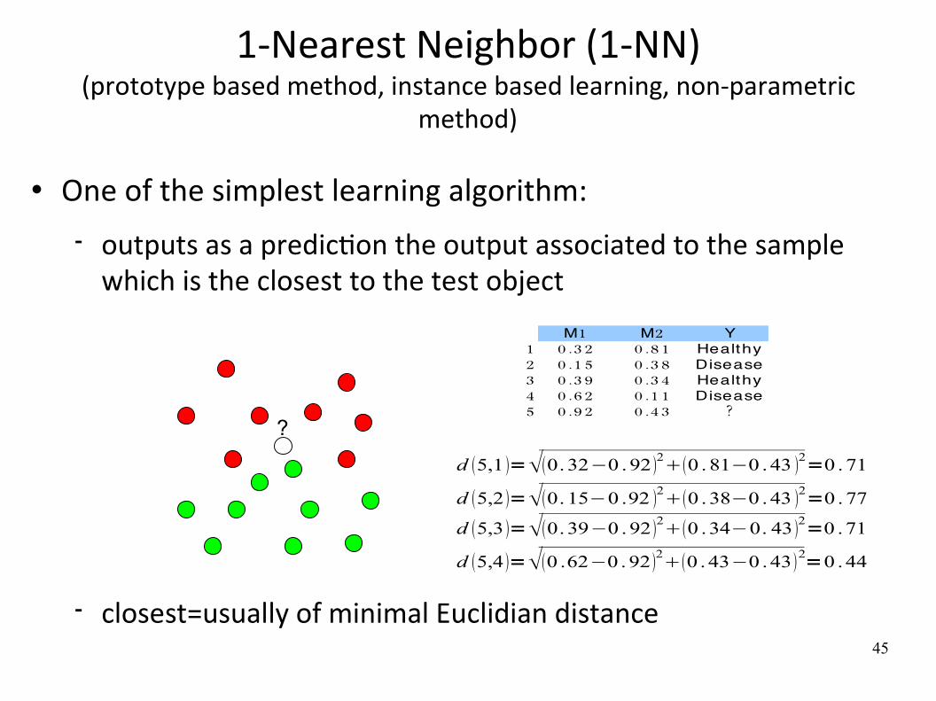
1‐Nearest Neighbor (1‐NN)(prototype based method, instance based learning, non‐parametric
method)
One of the simplest learning algorithm:
outputs as a predicWon the output associated to the sample which is the closest to the test object
closest=usually of minimal Euclidian distance
?
1M 2M Y1 0 .32 0 .81 Healthy2 0 .15 0 .38 Disease3 0 .39 0 .34 Healthy4 0 .62 0 .11 Disease5 0 .92 0 .43 ?
d 5,2 =0. 15−0 .92 20 . 38−0 . 43 2=0 . 77
d 5,3 =0. 39−0 . 92 20 .34−0. 43 2=0 .71
d 5,1 =0. 32−0 . 92 20 . 81−0 . 43 2=0 . 71
d 5,4 =0 .62−0 . 92 20 . 43−0 .43 2=0 . 44

46
Obvious extension: k‐NN
Find the k nearest neighbors (instead of only the first one) with respect to Euclidian distance
Output the most frequent class (classificaWon) or the average outputs (regression) among the k neighbors.
?
47
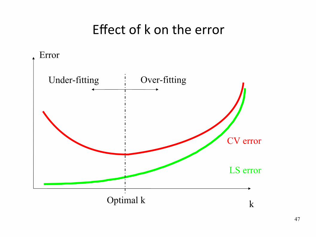
Effect of k on the error
Error
Over-fittingUnder-fitting
Optimal k k
CV error
LS error

48
Small exercise
Andrew Moore
In this classificaWon problem with two inputs:
What it the resubsWtuWon error (LS error) of 1‐NN?
What is the LOO error of 1‐NN? What is the LOO error of 3‐NN? What is the LOO error of 22‐NN?
49
k‐NN
Advantages:
very simple can be adapted to any data type by changing the distance measure
Drawbacks:
choosing a good distance measure is a hard problem very sensiWve to the presence of noisy variables slow for tesWng

50
Linear methods Find a model which is a linear combinaWons of the inputs
Regression:
ClassificaWon: if , otherwise
Several methods exist to find coefficients w0,w1... corresponding to different objecWve funcWons, opWmizaWon algorithms, eg.:
Regression: least‐square regression, ridge regression, parWal least square, support vector regression, LASSO...
ClassificaWon: linear discriminant analysis, PLS‐discriminant analysis, support vector machines...
y=w0w1 x1w2 x2...wn wn
y=c1 w0w1 x1...wn xn0 c2

51
Example: ridge regression
Find w that minimizes (λ>0):
From simple algebra, the soluWon is given by:
where X is the input matrix and y is the output vector λ regulates complexity (and avoids problems related to the singularity of XTX)
∑i yi−w x i2∥w∥2
w r=X T X I −1 X T y

52
Example: perceptron
Find w that minimizes:
using gradient descent: given a training example
Online algorithm, ie. that treats every example in turn (vs Batch algorithm that treats all examples at once)
Complexity is regulated by the learning rate η and the number of iteraWons
Can be adapted to classificaWon
∑i y i−w x i 2
y−wT x∀ j w j w j x j
x , y

53
Linear methods
Advantages:
simple there exist fast and scalable variants provide interpretable models through variable weights (magnitude and sign)
Drawbacks:
oFen not as accurate as other (non‐linear) methods

54
Non‐linear extensions GeneralizaWon of linear methods:
Any linear methods can be applied (but regularizaWon becomes more important)
ArWficial neural networks (with a single hidden layer):
where g is a non linear function (eg. sigmoid) (a non linear funcWon of a linear combinaWon of non linear funcWons of linear combinaWons of inputs)
Kernel methods:
where is the dot-product in the feature space and j indexes training examples
y=w0w11x w22 x2...wnn x
y=g ∑j
W j g ∑i
w i , j xi
y=∑i
w ii x ⇔ y=∑j j k x j , x
k x , x ' =⟨x ,x ' ⟩

55
ArWficial neural networks
Supervised learning method iniWally inspired by the behavior of the human brain
Consists of the inter‐connecWon of several small units EssenWally numerical but can handle classificaWon and discrete inputs with appropriate coding
Introduced in the late 50s, very popular in the 90s

56
Hypothesis space: a single neuron
X1
X2
XN
+ tanh
x w1
x w2
x wN
… Y
1
x w0
Y=tanh(w1*X1+w2*X2+…+wN*XN+w0)
X2
X1
+
_
-1
+1tanh
57
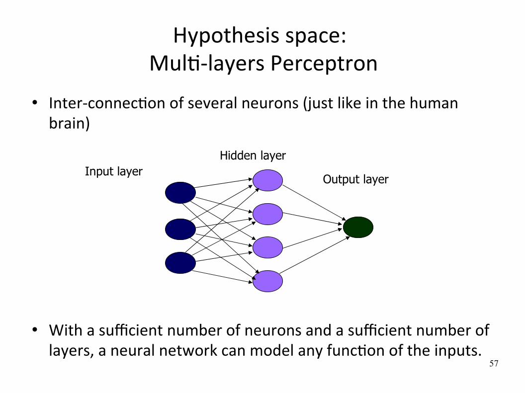
Hypothesis space: MulW‐layers Perceptron
Inter‐connecWon of several neurons (just like in the human brain)
With a sufficient number of neurons and a sufficient number of layers, a neural network can model any funcWon of the inputs.
Input layerHidden layer
Output layer
58
Learning
Choose a structure
Tune the value of the parameters (connecWons between neurons) so as to minimize the learning sample error.
Non‐linear opWmizaWon by the back‐propagaWon algorithm. In pracWce, quite slow.
Repeat for different structures
Select the structure that minimizes CV error

59
IllustraWve example
... ...
10 +10 neurons
2 +2 neurons
1 neuron
0
1
0 1X1
X2
0
1
0 1X1
X2
0
1
0 1X1
X2
60
ArWficial neural networks
Advantages: Universal approximators May be very accurate (if the method is well used)
Drawbacks:
The learning phase may be very slow Black‐box models, very difficult to interprete Scalability
61
Support vector machines
Recent (mid‐90's) and very successful method
Based on two smart ideas:
large margin classifier kernelized input space
62
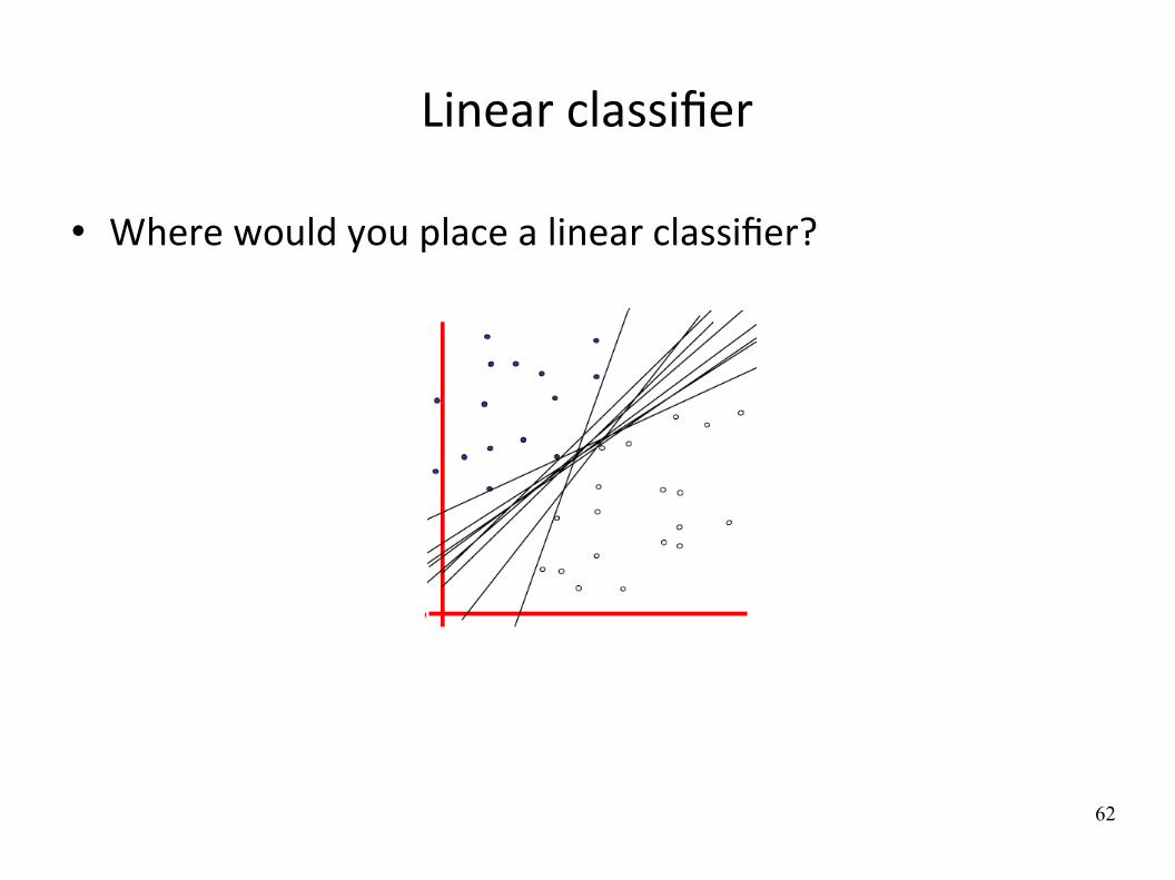
Linear classifier
Where would you place a linear classifier?
63
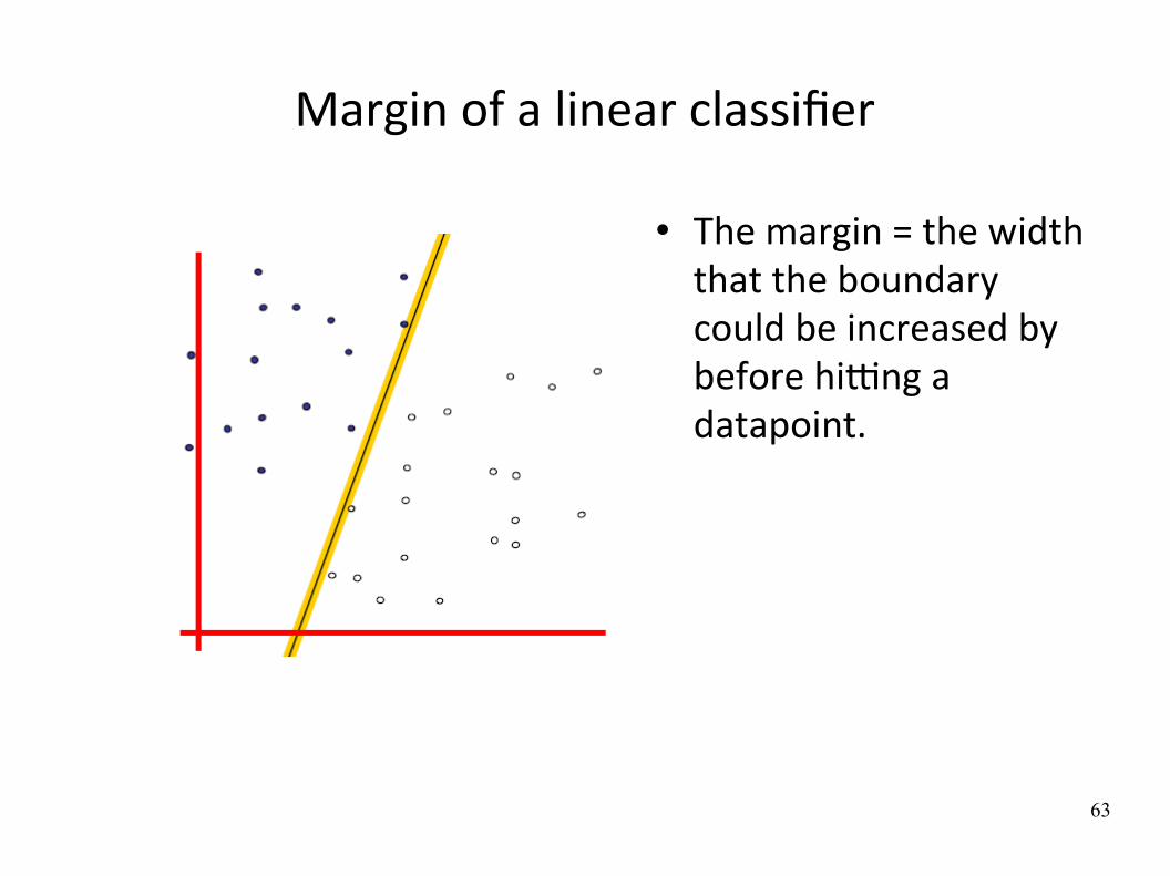
Margin of a linear classifier
The margin = the width that the boundary could be increased by before hiYng a datapoint.

64
Maximum‐margin linear classifier
The linear classifier with the maximum margin (= Linear SVM)
Why ?
IntuiWvely, safest Works very well TheoreWcal bounds: E(TS)<O(1/margin)
Kernel trickSupport vectors: the samples the closest to the hyperplane

65
MathemaWcally
Linearly separable case: amount at solving the following quadraWc programming opWmizaWon problem:
Decision funcWon:
if , otherwise
Non linearly separable case:
12∥w∥2
y i wT x i−b1,∀ i=1,. .. , N
minimize
subject to
y=−1wT x−b0y=1
12∥w∥2C∑
ii
y i wT x i−b1−i ,∀ i=1,. .. , N
minimize
subject to
66
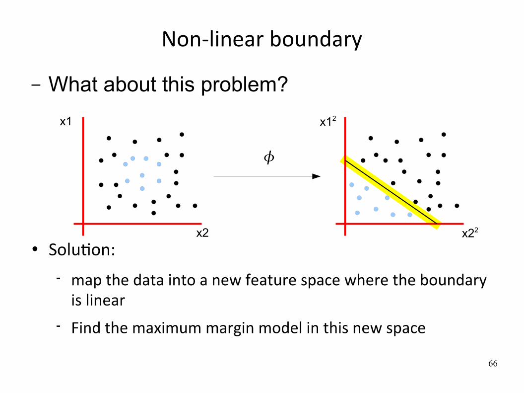
Non‐linear boundary
SoluWon:
map the data into a new feature space where the boundary is linear
Find the maximum margin model in this new space
– What about this problem?
x2
x1 x12
x22

67
MathemaWcally
Primal form of the opWmizaWon problem:
Dual form:
Decision funcWon:
if otherwise
12∥w∥2
y i ⟨w , xi⟩−b1,∀ i=1,. .. , N
minimizes
subject to
∑ii−
12∑i , j
i j yi y j ⟨ xi , x j⟩
i0
minimizes
subject to and
y=−1
⟨w , x ⟩=∑ii yi ⟨ xi , x ⟩0y=1
w=∑ii yi xi
∑ii y i=0
Depends only on dot-products between feature space vectors

68
The kernel trick
The maximum‐margin classifier in some feature space can be wriXen only in terms of dot‐products in that feature space:
You don't need to compute explicitly the mapping
All you need is a (special) similarity measure between objects (like for the kNN)
This similarity measure is called a kernel
MathemaWcally, a funcWon k is a valid (Mercer) kernel if the NxN (Gram) matrix K with K
i,j=k(x
i,x
j) is posiWve semi‐
definite for any subset of points {x1,...,x
N}.
⟨w , x ⟩=∑ii yi ⟨ xi , x ⟩=∑
ii y i k x i , x

69
Support vector machines
1X 2X Y1 0.49 0.94 1C2 0.86 0.59 2C3 0.6 0.79 2C4 0.83 0.66 1C5 0.63 0.27 1C6 -0.76 0.47 2C
1 2 3 4 5 61 1 0.14 0 .96 0 .17 0 .01 0 .242 0 .14 1 0 .02 0 .17 0 .22 0 .673 0 .96 0 .02 1 0 .15 0 .27 0 .074 0 .17 0 .7 0 .15 1 0 .37 0 .555 0 .01 0 .22 0 .27 0 .37 1 -0 .256 0 .24 0 .67 0 .07 0 .55 -0 .25 1
kernel matrix
Y1 1C2 2C3 2C4 1C5 1C6 2C
Class labels
SVM algorithm
Classificationmodel1X Y
1 ACGCTCTATAG 1C2 ACTCGCTTAGA 2C3 GTCTCTGAGAG 2C4 CGCTAGCGTCG 1C5 CGATCAGCAGC 1C6 GCTCGCGCTCG 2C

70
Examples of kernels
Linear kernel:
k(x,x')= <x,x'> Polynomial kernel
k(x,x')=(<x,x'>+1)d
(main parameter: d, the maximum degree)
Radial basis funcWon kernel:
k(x,x')=exp(-||x-x'||2/(22))
(main parameter: , the spread of the distribuWon)● + many kernels that have been defined for structured data types (eg. texts, graphs, trees, images)

71
Feature ranking with linear kernel
With a linear kernel, the model looks like:
Most important variables are those corresponding to large |wi|
h(x1,x2,...,xK)=C1 if w0+w1*x1+w2*x2+...+wK*xK>0C2 otherwise
0
20
40
60
80
100
variables
|w|

72
SVM parameters
Mainly two sets of parameters in SVM:
OpWmizaWon algorithm's parameters: Control the number of training errors versus the margin (when the learning sample is not linearly separable)
Kernel's parameters: choice of parWcular kernel given this choice, usually one complexity parameter eg, the degree of the polynomial kernel
Again, these parameters can be determined by cross‐validaWon

73
Support vector machines
Advantages: State‐of‐the‐art accuracy on many problems Can handle any data types by changing the kernel (many applicaWons on sequences, texts, graphs...)
Drawbacks:
Tuning the parameter is very crucial to get good results and somewhat tricky
Black‐box models, not easy to interprete

74
A note on kernel methods
The kernel trick can be applied to any (learning) algorithm whose soluWon can be expressed in terms of dot‐products in the original input space
It makes a non‐linear algorithm from a linear one Can work in a very highly dimensional space (even infinite) without requiring to explicitly compute the features
Decouple the representaWon stage from the learning stage. The same learning machine can be applied to a large range of problems
Examples: ridge regression, perceptron, PCA, k‐means...
75
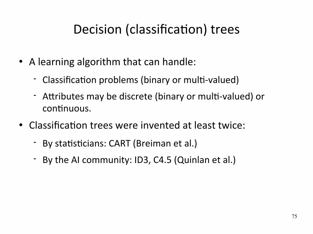
Decision (classificaWon) trees
A learning algorithm that can handle:
ClassificaWon problems (binary or mulW‐valued) AXributes may be discrete (binary or mulW‐valued) or conWnuous.
ClassificaWon trees were invented at least twice:
By staWsWcians: CART (Breiman et al.) By the AI community: ID3, C4.5 (Quinlan et al.)
76
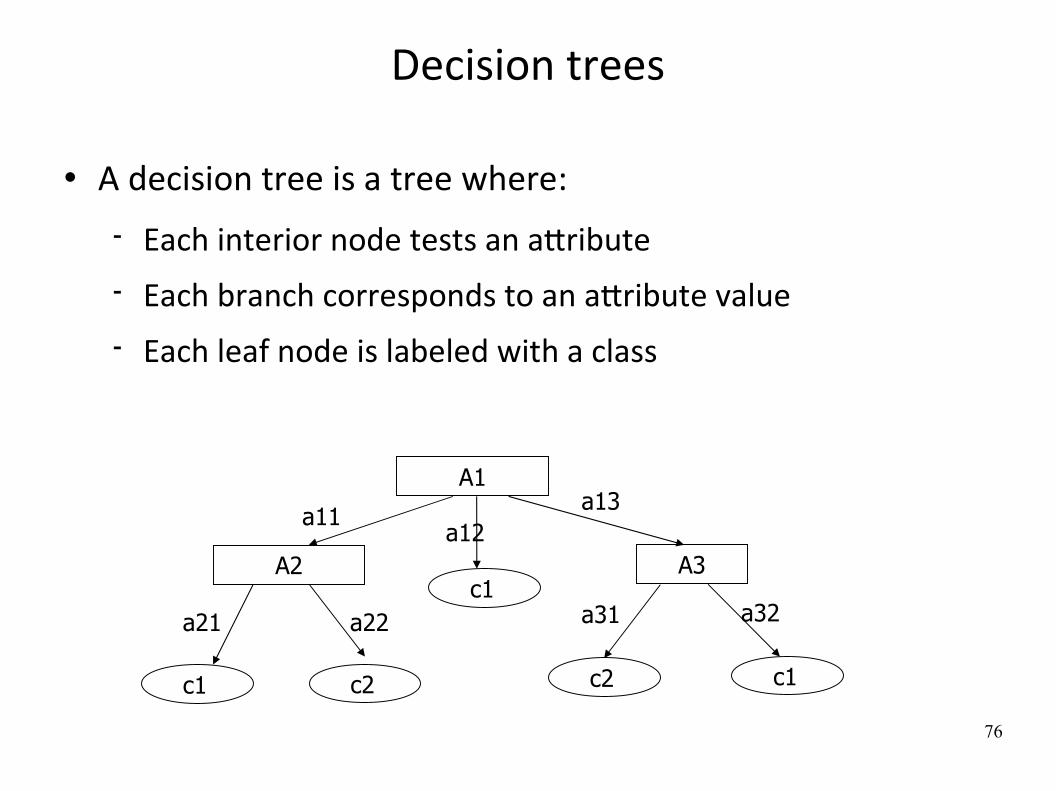
Decision trees
A decision tree is a tree where:
Each interior node tests an aXribute Each branch corresponds to an aXribute value Each leaf node is labeled with a class
A1
A2 A3
c1 c2
c1
c2 c1
a11a12
a13
a21 a22 a31 a32

77
A simple database: playtennis
NoStrongHighMildRainD14
YesStrongHighMildOvercastD12YesWeakNormalHotOvercastD13
YesStrongNormalMildRainD10YesWeakNormalHotSunnyD9
YesStrongNormalCoolSunnyD11
YesWeakNormalCoolRainD5NoStrongNormalCoolRainD6YesStrongHighCoolOvercastD7NoWeakNormalMildSunnyD8
RainOvercastSunnySunny
Outlook
YesWeakNormalMildD4YesWeakHighHotD3NoStrongHighHotD2NoWeakHighHotD1
Play TennisWindHumidityTemperatureDay

78
A decision tree for playtennis
Outlook
Humidity Wind
no yes
yes
no yes
SunnyOvercast
Rain
High Normal Strong Weak
SunnyOutlook
?WeakHighHotD15Play TennisWindHumidityTemperatureDay
Should we play tennis on D15?
79
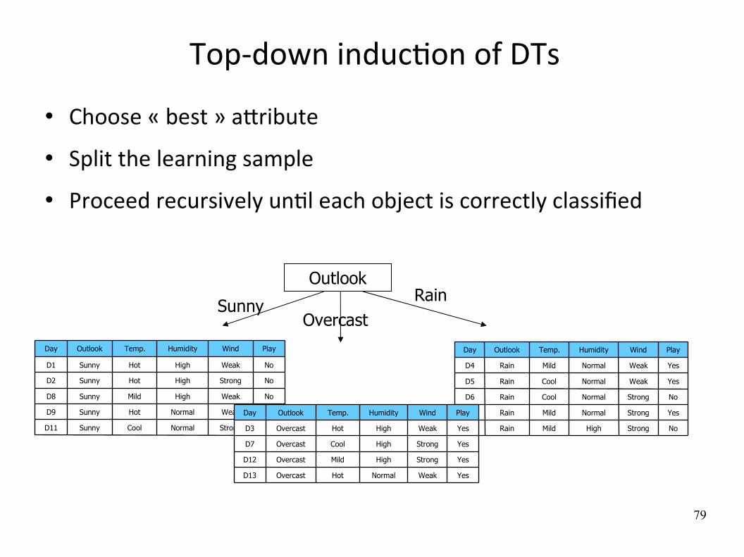
Top‐down inducWon of DTs
Choose « best » aXribute
Split the learning sample
Proceed recursively unWl each object is correctly classified
Outlook
SunnyOvercast
Rain
YesWeakNormalHotSunnyD9
YesStrongNormalCoolSunnyD11
NoWeakHighMildSunnyD8
Sunny
Sunny
Outlook
NoStrongHighHotD2
NoWeakHighHotD1
PlayWindHumidityTemp.Day
YesStrongNormalMildRainD10
NoStrongHighMildRainD14
NoStrongNormalCoolRainD6
YesWeakNormalCoolRainD5
Rain
Outlook
YesWeakNormalMildD4
PlayWindHumidityTemp.Day
YesStrongHighMildOvercastD12
YesWeakNormalHotOvercastD13
YesStrongHighCoolOvercastD7
Overcast
Outlook
YesWeakHighHotD3
PlayWindHumidityTemp.Day

80
Top‐down inducWon of DTs
Procedure learn_dt(learning sample, LS) If all objects from LS have the same class
Create a leaf with that class Else
Find the « best » spliYng aXribute A Create a test node for this aXribute For each value a of A
Build LSa= {o LS | A(o) is a} Use Learn_dt(LSa) to grow a subtree from LSa.

81
Which aXribute is best ?
A “score” measure is defined to evaluate splits
This score should favor class separaWon at each step (to shorten the tree depth)
Common score measures are based on informaWon theory
A1=?
T F
[21+,5-] [8+,30-]
[29+,35-] A2=?
T F
[18+,33-] [11+,2-]
[29+,35-]
leftleft LSHLS
LSLSHALSI )(||||)(),( rightright LSH
LSLS )(
||||
82
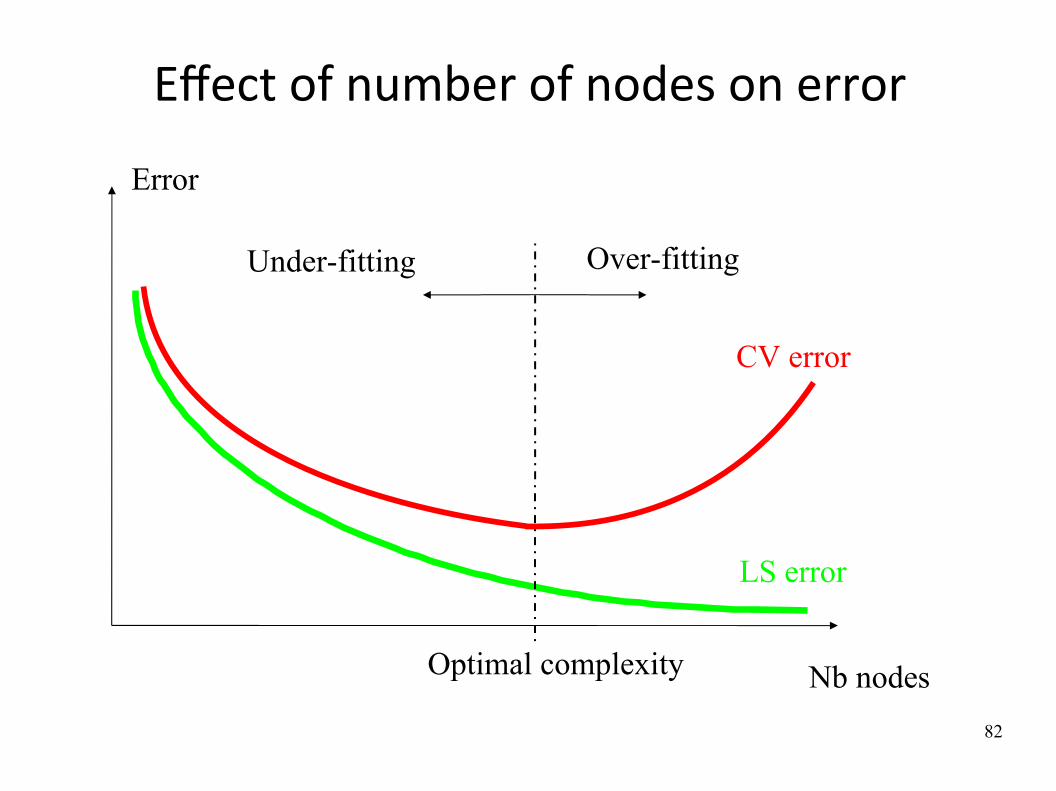
Effect of number of nodes on error
Error
Over-fittingUnder-fitting
Optimal complexity Nb nodes
CV error
LS error
83
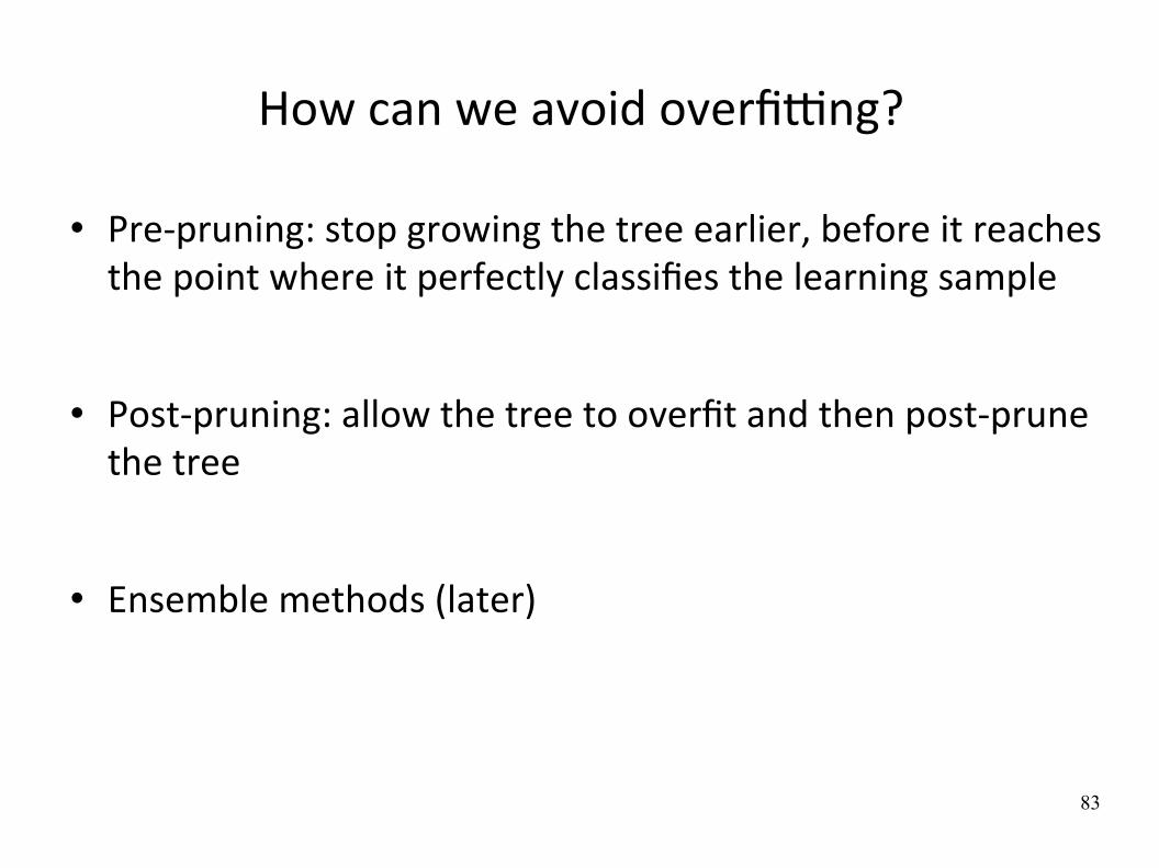
How can we avoid overfiYng?
Pre‐pruning: stop growing the tree earlier, before it reaches the point where it perfectly classifies the learning sample
Post‐pruning: allow the tree to overfit and then post‐prune the tree
Ensemble methods (later)
84
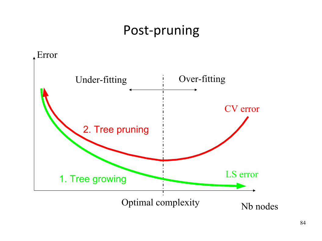
Post‐pruning
Error
Over-fittingUnder-fitting
Optimal complexity Nb nodes
LS error1. Tree growing
CV error
2. Tree pruning
85
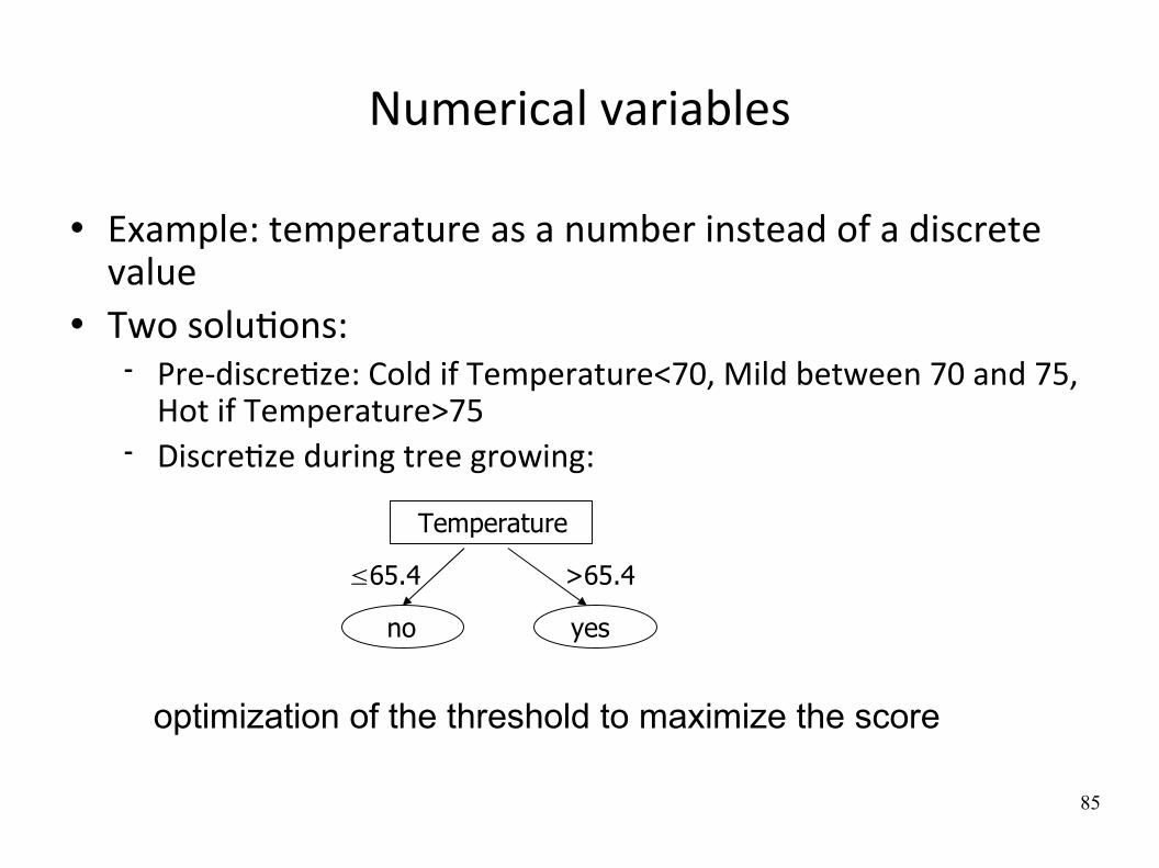
Numerical variables
Example: temperature as a number instead of a discrete value
Two soluWons: Pre‐discreWze: Cold if Temperature<70, Mild between 70 and 75, Hot if Temperature>75
DiscreWze during tree growing:
optimization of the threshold to maximize the score
Temperature
no yes
65.4 >65.4

86
IllustraWve example
X2<0.33?
Healthy X1<0.91?
X1<0.23? X2<0.91?
X2<0.75?X2<0.49?
X2<0.65?Healthy
Sick Healthy
Sick
Sick
Sick
Healthy
yes no
0
1
0 1X1
X2

87
Regression trees
Trees for regression problems: exactly the same model but with a number in each leaf instead of a class
1.2
Outlook
Humidity Wind
22.3
45.6
64.4 7.4
SunnyOvercast
Rain
High Normal Strong Weak
Temperature
3.4
<71 >71
88
Interpretability and aXribute selecWon
Interpretability Intrinsically, a decision tree is highly interpretable A tree may be converted into a set of “if…then” rules.
AXribute selecWon If some aXributes are not useful for classificaWon, they will not be selected in the (pruned) tree
Of pracWcal importance, if measuring the value of a variable is costly (e.g. medical diagnosis)
Decision trees are oFen used as a pre‐processing for other learning algorithms that suffer more when there are irrelevant variables

89
AXribute importance
In many applicaWons, all variables do not contribute equally in predicWng the output.
We can evaluate variable importances with trees
Outlook
Humidity
Wind
Temperature
90
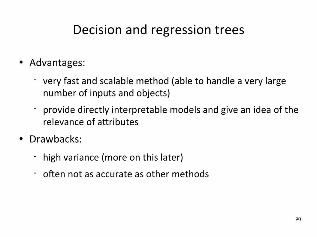
Decision and regression trees
Advantages:
very fast and scalable method (able to handle a very large number of inputs and objects)
provide directly interpretable models and give an idea of the relevance of aXributes
Drawbacks:
high variance (more on this later) oFen not as accurate as other methods
91
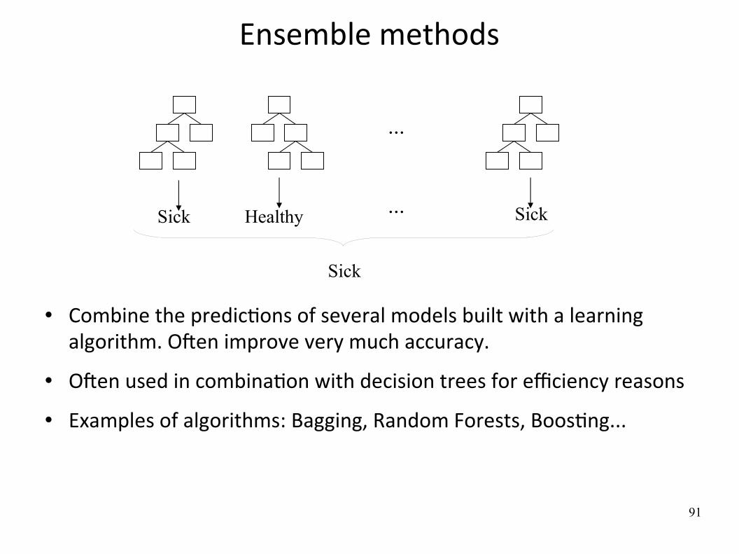
Ensemble methods
Combine the predicWons of several models built with a learning algorithm. OFen improve very much accuracy.
OFen used in combinaWon with decision trees for efficiency reasons
Examples of algorithms: Bagging, Random Forests, BoosWng...
...
Healthy SickSick ...
Sick

92
Bagging: moWvaWon
Different learning samples yield different models, especially when the learning algorithm overfits the data
As there is only one opWmal model, this variance is source of error
SoluWon: aggregate several models to obtain a more stable one
0
1
0 10
1
0 1
0
1
0 1

93
Bagging: bootstrap aggregaWng
Boostrap sampling
(sampling with replacement)
Note: the more models, the better.
0
0 0 0
...1
...
Sick
Healthy SickSick ...

94
Bootstrap sampling
1G 2G Y1 0 .74 0 .68 Healthy2 0 .78 0 .45 Disease3 0 .86 0 .09 Healthy4 0 .2 0 .61 Disease5 0 .2 -5 .6 Healthy6 0 .32 0 .6 Disease7 -0 .34 -0 .45 Healthy8 0 .89 -0 .34 Disease9 0 .1 0 .3 Healthy
10 -0 .34 -0 .65 Healthy
1G 2G Y3 0 .86 0 .09 Healthy7 -0 .34 -0 .45 Healthy2 0 .78 0 .45 Disease9 0 .1 0 .3 Healthy3 0 .86 0 .09 Healthy
10 -0 .34 -0 .65 Healthy1 0 .74 0 .68 Healthy8 0 .89 -0 .34 Disease6 0 .32 0 .6 Disease
10 -0 .34 -0 .65 Healthy
Sampling with replacement
Some objects do not appear, some objects appear several Wmes

95
BoosWng
Idea of boosWng: combine many « weak » models to produce a more powerful one.
Weak model = a model that underfits the data (strictly, in classificaWon, a model slightly beXer than random guessing)
Adaboost: At each step, adaboost forces the learning algorithm to focus on the cases from the learning sample misclassified by the last model
Eg., by duplicaWng the missclassified examples in the learning sample
The predicWons of the models are combined through a weighted vote. More accurate models have more weights in the vote.

96
BoosWng
LS
LS1 LS2
Healthy Sick Healthy
w1 w2wT
Healthy
LST
…
…
...

97
Interpretability and efficiency
When combined with decision trees, ensemble methods loose interpretability and efficiency
However,
We sWll can use the ensemble to compute the importance of variables (by averaging it over all trees)
Ensemble methods can be parallelized and boosWng type algorithm uses smaller trees. So, the increase of compuWng Wmes is not so detrimental.
0
20
40
60
80
100
98
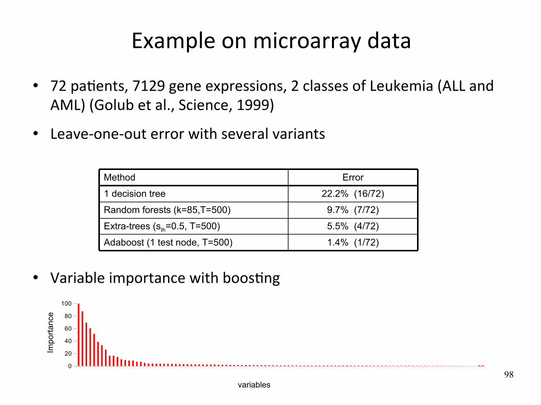
Example on microarray data
72 paWents, 7129 gene expressions, 2 classes of Leukemia (ALL and AML) (Golub et al., Science, 1999)
Leave‐one‐out error with several variants
Variable importance with boosWng
9.7% (7/72)Random forests (k=85,T=500)
1.4% (1/72)Adaboost (1 test node, T=500)
5.5% (4/72)Extra-trees (sth=0.5, T=500)
ErrorMethod
22.2% (16/72)1 decision tree
0
20
40
60
80
100
Impo
rtanc
e
variables

99
Method comparison
Method Accuracy Efficiency Interpretability Ease of use
kNN ++ + + ++
DT + +++ +++ +++
Linear ++ +++ ++ +++
Ensemble +++ +++ ++ +++
ANN +++ + + ++
SVM ++++ + + +
Note:
The relaWve importance of the criteria depends on the specific applicaWon
These are only general trends. Eg., in terms of accuracy, no algorithm is always beXer than all others.

100
Outline
● IntroducWon
● Supervised Learning
IntroducWon Model selecWon, cross‐validaWon, overfiYng Some supervised learning algorithms Beyond classificaWon and regression
● Other learning protocols/frameworks
101
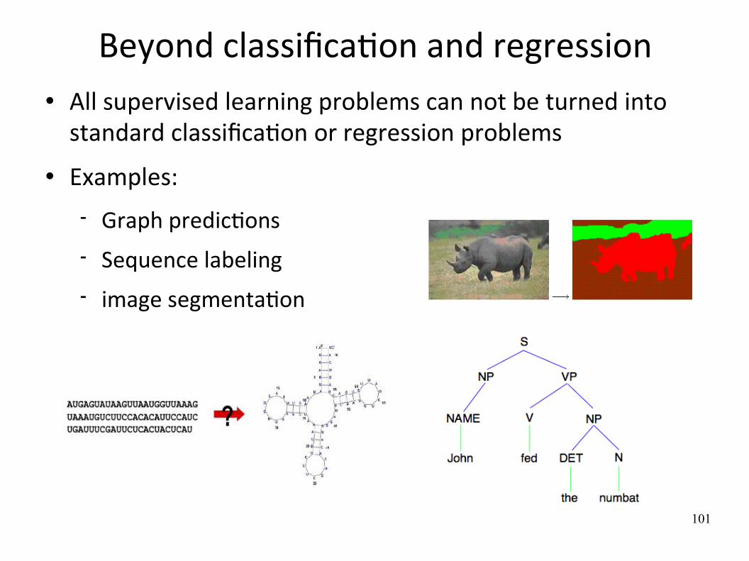
Beyond classificaWon and regression All supervised learning problems can not be turned into standard classificaWon or regression problems
Examples:
Graph predicWons Sequence labeling image segmentaWon
102
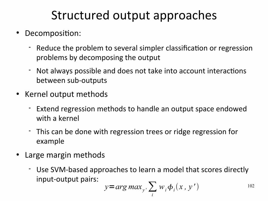
Structured output approaches DecomposiWon:
Reduce the problem to several simpler classificaWon or regression problems by decomposing the output
Not always possible and does not take into account interacWons between sub‐outputs
Kernel output methods
Extend regression methods to handle an output space endowed with a kernel
This can be done with regression trees or ridge regression for example
Large margin methods
Use SVM‐based approaches to learn a model that scores directly input‐output pairs:
y=arg maxy '∑
iw ii x , y '
103
Outline
IntroducWon
Supervised learning
Other learning protocols/frameworks
● Semi‐supervised learning
● TransducWve learning
● AcWve learning
● Reinforcement learning
● Unsupervised learning
104
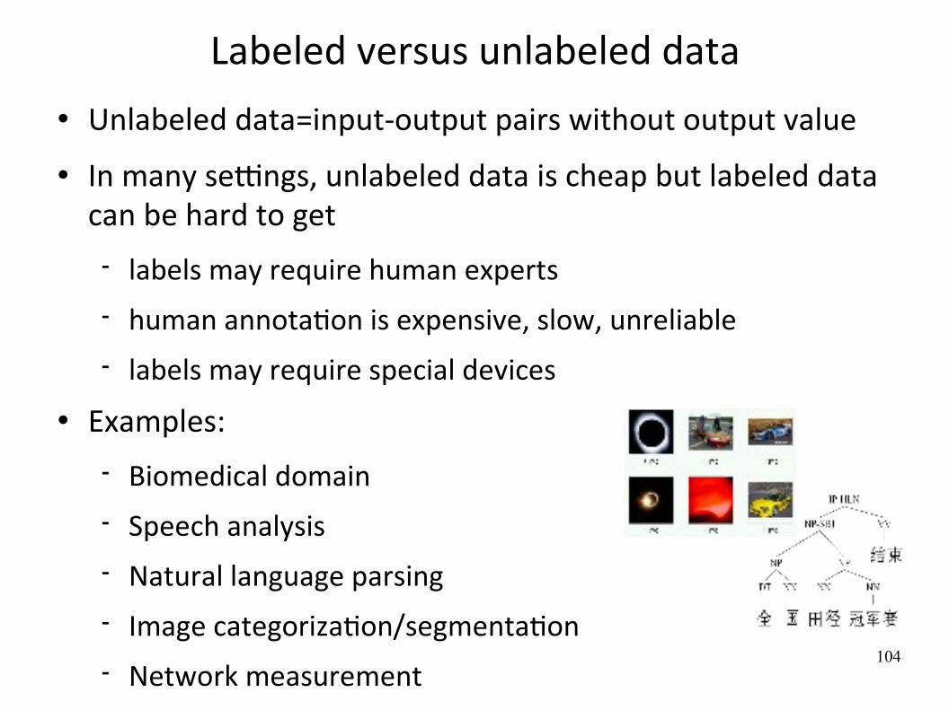
Labeled versus unlabeled data Unlabeled data=input‐output pairs without output value
In many seYngs, unlabeled data is cheap but labeled data can be hard to get
labels may require human experts human annotaWon is expensive, slow, unreliable labels may require special devices
Examples:
Biomedical domain Speech analysis Natural language parsing Image categorizaWon/segmentaWon Network measurement

105
Semi‐supervised learning Goal: exploit both labeled and unlabeled data to build beXer models than using each one alone
Why would it improve?
1A 2A 3A 4A Y0 .01 0 .37 T 0 .54 Healthy-2 .3 -1 .2 F 0 .37 Disease0 .69 -0 .78 F 0 .63 Healthy-0 .56 -0 .89 T -0 .42-0 .85 0 .62 F -0 .05-0 .17 0 .09 T 0 .29-0 .09 0 .3 F 0 .17 ?
labeled data
unlabeled data
test data
106
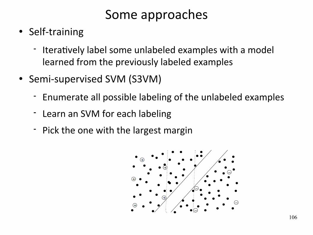
Some approaches Self‐training
IteraWvely label some unlabeled examples with a model learned from the previously labeled examples
Semi‐supervised SVM (S3VM)
Enumerate all possible labeling of the unlabeled examples Learn an SVM for each labeling Pick the one with the largest margin

107
Some approaches
Graph‐based algorithms
Build a graph over the (labeled and unlabeled) examples (from the inputs)
Learn a model that predicts well labeled examples and is smooth over the graph

108
TransducWve learning
Like supervised learning but we have access to the test data from the beginning and we want to exploit it
We don't want a model, only compute predicWons for the unlabeled data
Simple soluWon:
Apply semi‐supervised learning techniques using the test data as unlabeled data to get a model
Use the resulWng model to make predicWons on the test data
There exist also specific algorithms that avoid building a model

109
AcWve learning Goal:
given unlabeled data, find (adapWvely) the examples to label in order to learn an accurate model
The hope is to reduce the number of labeled instances with respect to the standard batch SL
Usually, in an online seYng:
choose the k “best” unlabeled examples determine their labels update the model and iterate
Algorithms differ in the way the unlabeled examples are selected
Example: choose the k examples for which the model predicWons are the most uncertain
110
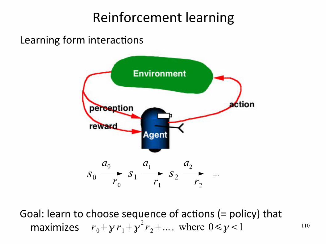
Reinforcement learning
Learning form interacWons
Goal: learn to choose sequence of acWons (= policy) that maximizes
s0
a0
r0s1
a1
r1
s2
a2
r2
...
r0 r12 r2... , where 01

111
RL approaches
System is usually modeled by
state transiWon probabiliWes reward probabiliWes
(= Markov Decision Process) Model of the dynamics and reward is known ⇒ try to compute opWmal policy by dynamic programming
Model is unknown
Model‐based approaches ⇒ first learn a model of the dynamics and then derive an opWmal policy from it (DP)
Model‐free approaches ⇒ learn directly a policy from the observed system trajectories
P st1∣st , at
P r t1∣st , at
112
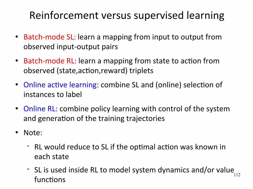
Reinforcement versus supervised learning
Batch‐mode SL: learn a mapping from input to output from observed input‐output pairs
Batch‐mode RL: learn a mapping from state to acWon from observed (state,acWon,reward) triplets
Online acWve learning: combine SL and (online) selecWon of instances to label
Online RL: combine policy learning with control of the system and generaWon of the training trajectories
Note:
RL would reduce to SL if the opWmal acWon was known in each state
SL is used inside RL to model system dynamics and/or value funcWons

113
Examples of applicaWons
Robocup Soccer Teams (Stone & Veloso, Riedmiller et al.)
Inventory Management (Van Roy, Bertsekas, Lee &Tsitsiklis)
Dynamic Channel Assignment, RouWng (Singh & Bertsekas, Nie & Haykin, Boyan & LiXman)
Elevator Control (Crites & Barto)
Many Robots: navigaWon, bi‐pedal walking, grasping, switching between skills...
Games: TD‐Gammon and Jellyfish (Tesauro, Dahl)

114
Robocup
Goal: by the year 2050, develop a team of fully autonomous humanoid robots that can win against the human world soccer champion team.
http://www.robocup.orghttp://www.youtube.com/watch?v=v-ROG5eEdIk

116
Unsupervised learning
Unsupervised learning tries to find any regulariWes in the data without guidance about inputs and outputs
Are there interesWng groups of variables or samples? outliers? What are the dependencies between variables?
1A 2A 3A 4A 5A 6A 7A 8A 9A 10A 11A 12A 13A 14A 15A 16A 17A 18A 19A-0.27 -0.15 -0.14 0.91 -0.17 0.26 -0.48 -0.1 -0.53 -0.65 0.23 0.22 0.98 0.57 0.02 -0.55 -0.32 0.28 -0.33-2.3 -1.2 -4.5 -0.01 -0.83 0.66 0.55 0.27 -0.65 0.39 -1.3 -0.2 -3.5 0.4 0.21 -0.87 0.64 0.6 -0.290.41 0.77 -0.44 0 0.03 -0.82 0.17 0.54 -0.04 0.6 0.41 0.66 -0.27 -0.86 -0.92 0 0.48 0.74 0.490.28 -0.71 -0.82 0.27 -0.21 -0.9 0.61 -0.57 0.44 0.21 0.97 -0.27 0.74 0.2 -0.16 0.7 0.79 0.59 -0.33-0.28 0.48 0.79 -0.14 0.8 0.28 0.75 0.26 0.3 -0.78 -0.72 0.94 -0.78 0.48 0.26 0.83 -0.88 -0.59 0.710.01 0.36 0.03 0.03 0.59 -0.5 0.4 -0.88 -0.53 0.95 0.15 0.31 0.06 0.37 0.66 -0.34 0.79 -0.12 0.49-0.53 -0.8 -0.64 -0.93 -0.51 0.28 0.25 0.01 -0.94 0.96 0.25 -0.12 0.27 -0.72 -0.77 -0.31 0.44 0.58 -0.860.04 0.94 -0.92 -0.38 -0.07 0.98 0.1 0.19 -0.57 -0.69 -0.23 0.05 0.13 -0.28 0.98 -0.08 -0.3 -0.84 0.47-0.88 -0.73 -0.4 0.58 0.24 0.08 -0.2 0.42 -0.61 -0.13 -0.47 -0.36 -0.37 0.95 -0.31 0.25 0.55 0.52 -0.66-0.56 0.97 -0.93 0.91 0.36 -0.14 -0.9 0.65 0.41 -0.12 0.35 0.21 0.22 0.73 0.68 -0.65 -0.4 0.91 -0.64

117
Unsupervised learning methods
Many families of problems exist, among which:
Clustering: try to find natural groups of samples/variables eg: k‐means, hierarchical clustering
Dimensionality reducWon: project the data from a high‐dimensional space down to a small number of dimensions
eg: principal/independent component analysis, MDS Density esWmaWon: determine the distribuWon of data within the input space
eg: bayesian networks, mixture models.

118
Clustering
Goal: grouping a collecWon of objects into subsets or “clusters”, such that those within each cluster are more closely related to one another than objects assigned to different clusters
119
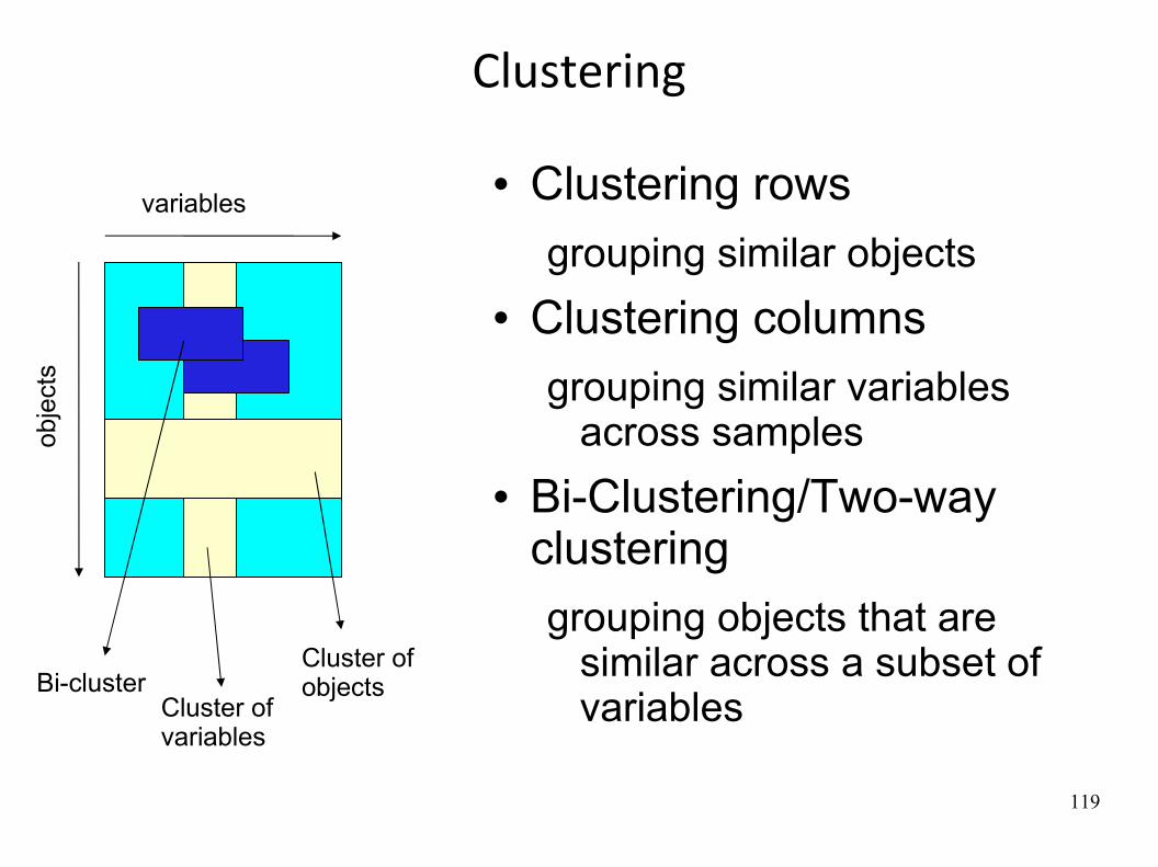
Clustering
Clustering rows grouping similar objects
Clustering columnsgrouping similar variables
across samples Bi-Clustering/Two-way
clusteringgrouping objects that are
similar across a subset of variables
variables
obje
cts
Cluster of objectsBi-cluster
Cluster of variables
120
ApplicaWons of clustering
MarkeWng: finding groups of customers with similar behavior given a large database of customer data containing their properWes and past buying records;
Biology: classificaWon of plants and animals given their features;
Insurance: idenWfying groups of motor insurance policy holders with a high average claim cost; idenWfying frauds;
City‐planning: idenWfying groups of houses according to their house type, value and geographical locaWon;
Earthquake studies: clustering observed earthquake epicenters to idenWfy dangerous zones;
WWW: document classificaWon; clustering weblog data to discover groups of similar access paXerns.

121
Clustering
Two essenWal components of cluster analysis:
Distance measure: A noWon of distance or similarity of two objects: When are two objects close to each other?
Cluster algorithm: A procedure to minimize distances of objects within groups and/or maximize distances between groups

122
Examples of distance measures
Euclidean distance measures average difference across coordinates
Manha5an distance measures average difference across coordinates, in a robust way
Correla4on distance measures difference with respect to trends

123
Comparison of the distances
All distances are normalized to the interval [0,10] and then rounded

124
Clustering algorithms
Popular algorithms for clustering
hierarchical clustering K‐means SOMs (Self‐Organizing Maps) autoclass, mixture models...
Hierarchical clustering allows the choice of the dissimilarity matrix.
k‐Means and SOMs take original data directly as input. AXributes are assumed to live in Euclidean space.
125
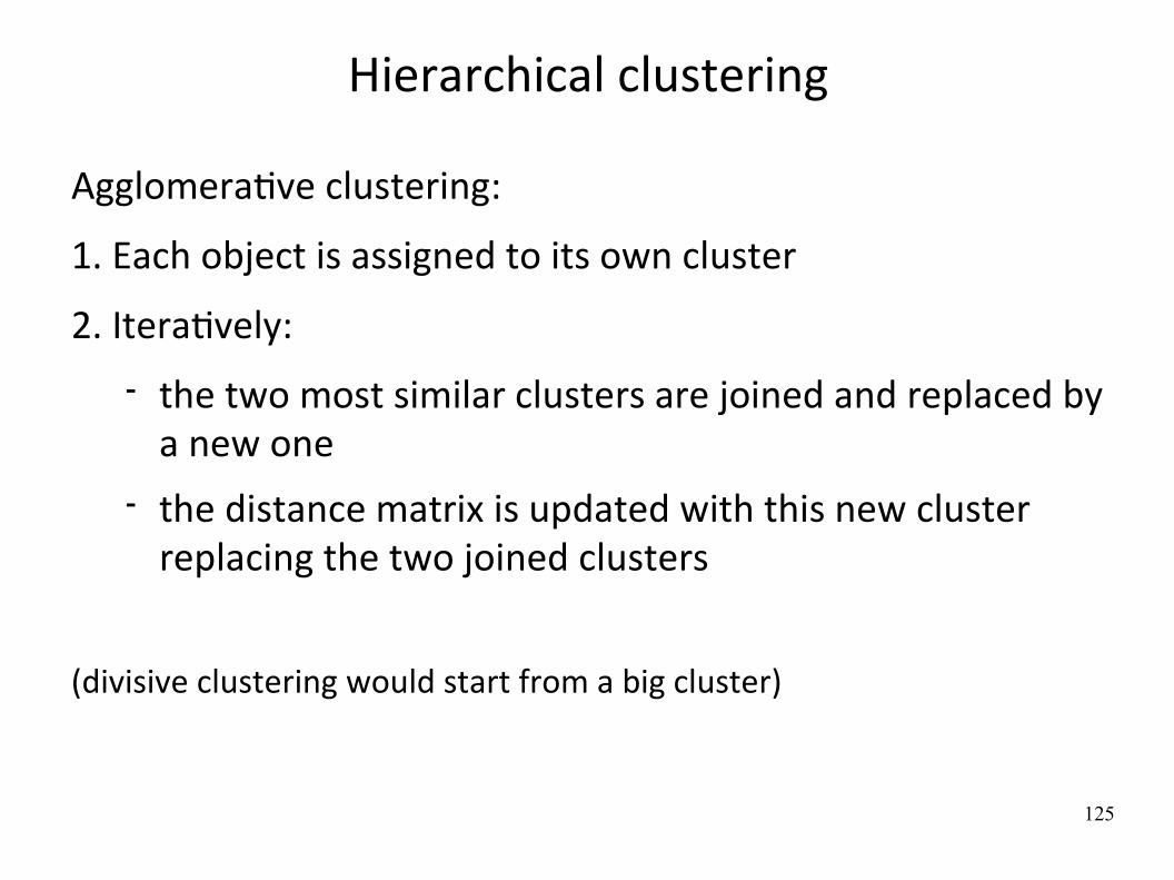
Hierarchical clustering
AgglomeraWve clustering:
1. Each object is assigned to its own cluster
2. IteraWvely:
the two most similar clusters are joined and replaced by a new one
the distance matrix is updated with this new cluster replacing the two joined clusters
(divisive clustering would start from a big cluster)
126
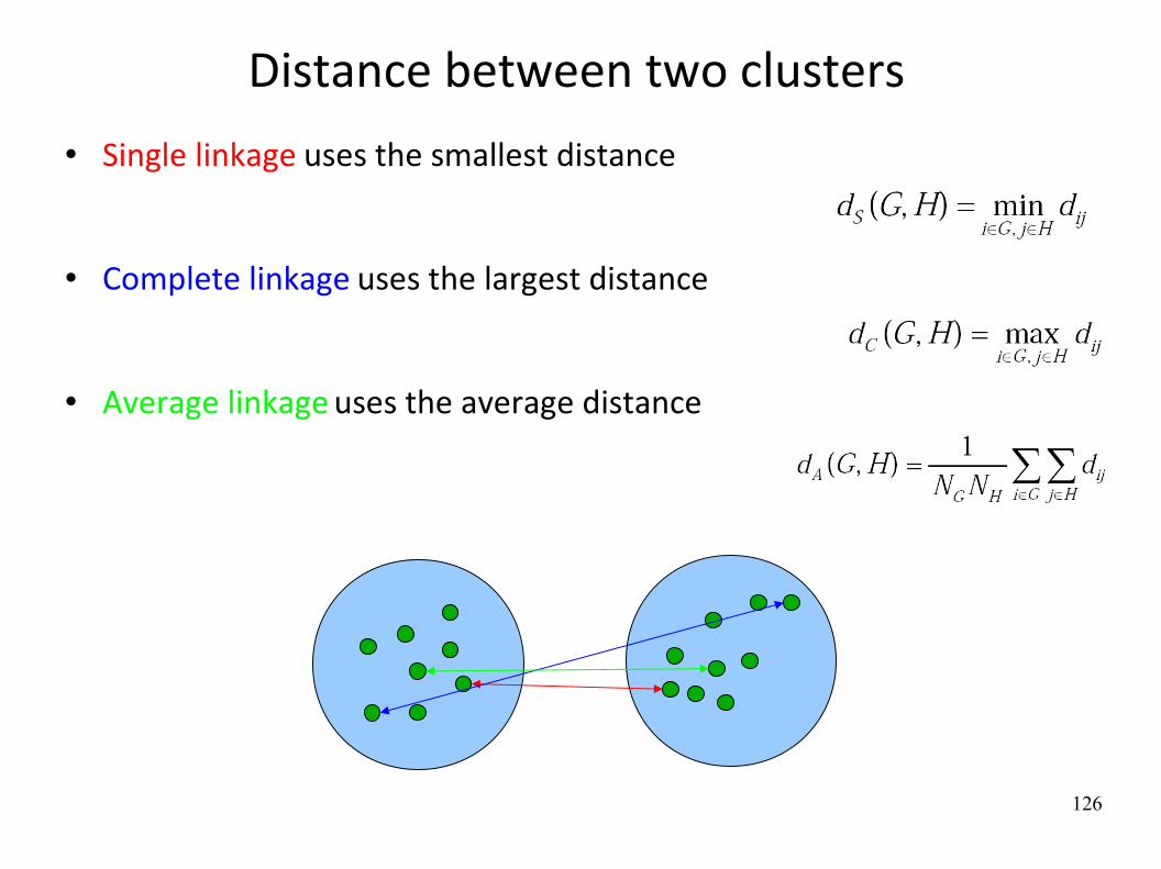
Distance between two clusters Single linkage uses the smallest distance
Complete linkage uses the largest distance
Average linkage uses the average distance
127
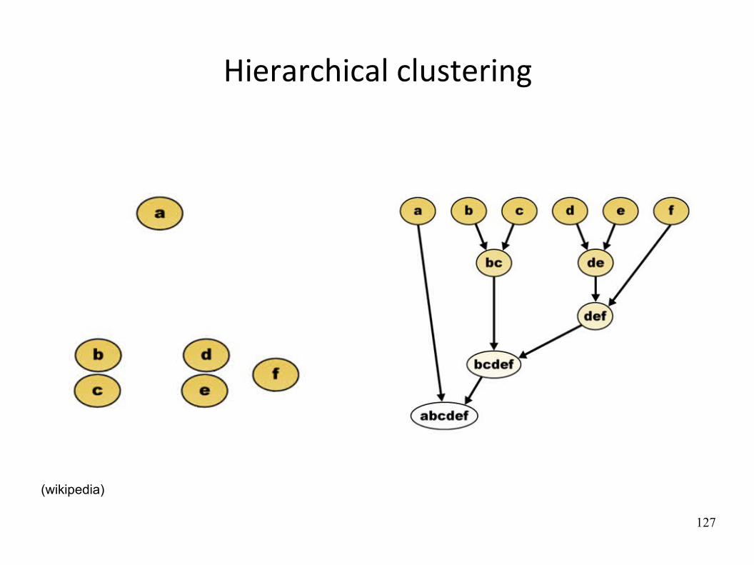
Hierarchical clustering
(wikipedia)
128
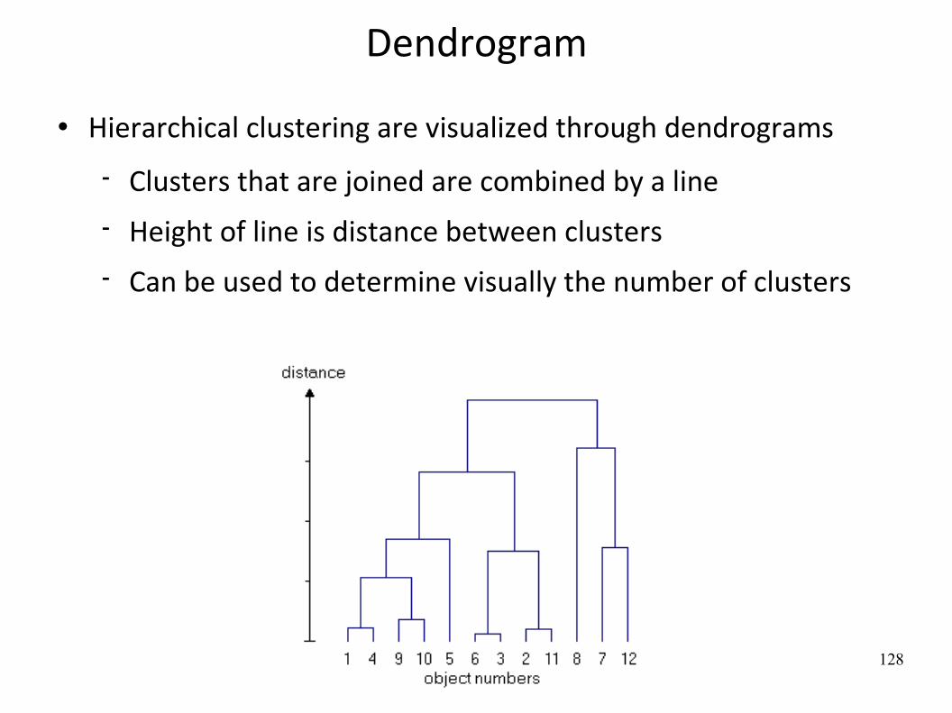
Dendrogram
Hierarchical clustering are visualized through dendrograms
Clusters that are joined are combined by a line Height of line is distance between clusters Can be used to determine visually the number of clusters

129
IllustraWons (1)
Breast cancer data (Langerød et al., Breast cancer, 2007)
80 tumor samples (wild‐type,TP53 mutated), 80 genes

130
IllustraWons (2)Assfalg et al., PNAS, Jan 2008
Evidence of different metabolic phenotypes in humans
Urine samples of 22 volunteers over 3 months, NMR spectra analysed by HCA

131
Hierarchical clustering Strengths
No need to assume any parWcular number of clusters Can use any distance matrix Find someWmes a meaningful taxonomy
LimitaWons
Find a taxonomy even if it does not exist Once a decision is made to combine two clusters it cannot be undone
Not well theoreWcally moWvated

132
k‐Means clustering
ParWWoning algorithm with a prefixed number k of clusters Use Euclidean distance between objects
Try to minimize the sum of intra‐cluster variances
where cj is the center of cluster j and d2 is the Euclidean distance
∑j=1
k
∑o∈Cluster j
d 2 o,c j

133
k‐Means clustering

134
k‐Means clustering

135
k‐Means clustering

136
k‐Means clustering
Strengths
Simple, understandable Can cluster any new point (unlike hierarchical clustering) Well moWvated theoreWcally
LimitaWons
Must fix the number of clusters beforehand SensiWve to the iniWal choice of cluster centers SensiWve to outliers
137
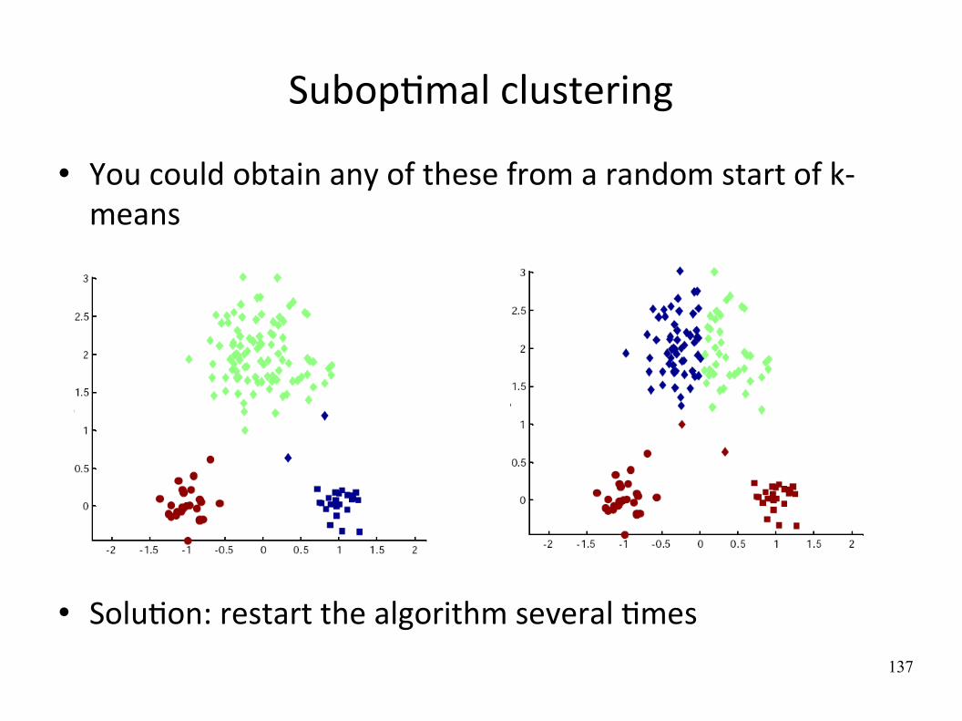
SubopWmal clustering
You could obtain any of these from a random start of k‐means
SoluWon: restart the algorithm several Wmes

138
ApplicaWon: vector quanWzaWon
139
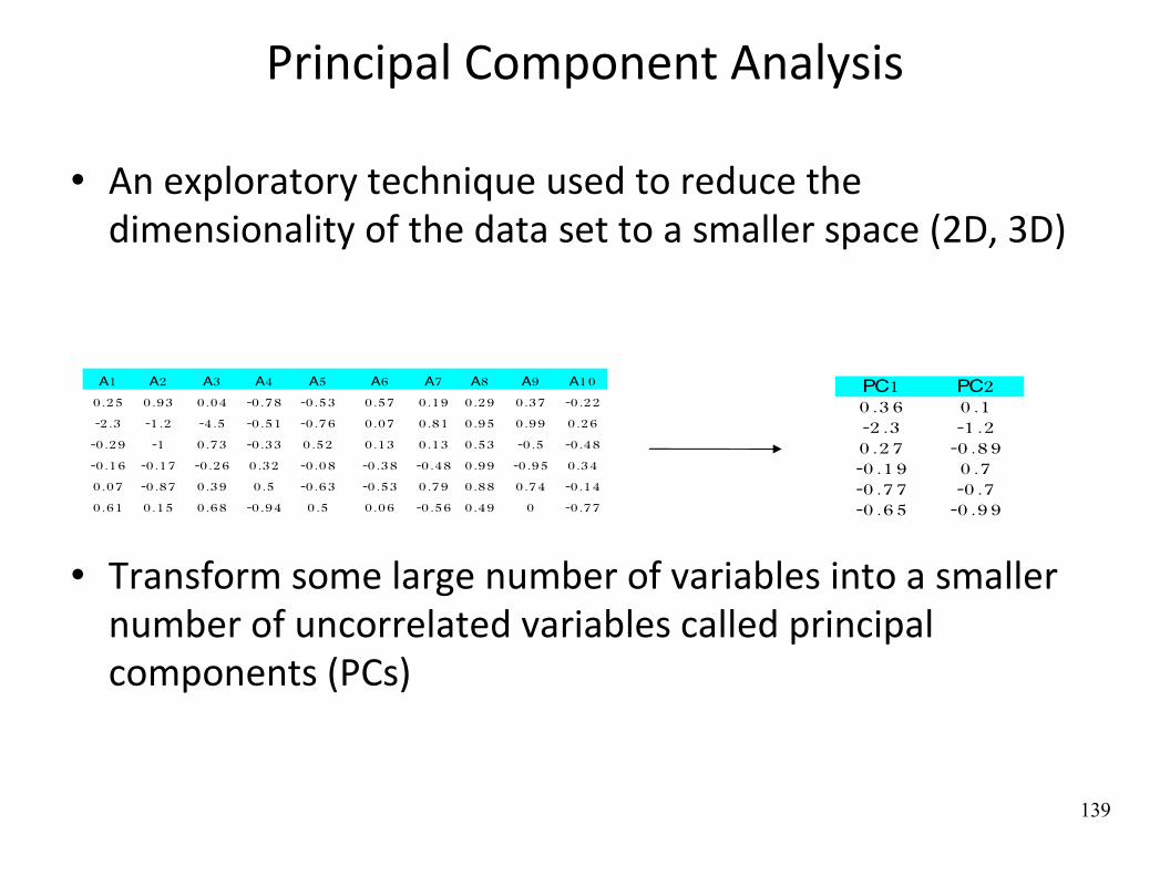
Principal Component Analysis
An exploratory technique used to reduce the dimensionality of the data set to a smaller space (2D, 3D)
Transform some large number of variables into a smaller number of uncorrelated variables called principal components (PCs)
1A 2A 3A 4A 5A 6A 7A 8A 9A 10A0.25 0.93 0.04 -0.78 -0.53 0.57 0.19 0.29 0.37 -0.22-2.3 -1.2 -4.5 -0.51 -0.76 0.07 0.81 0.95 0.99 0.26-0.29 -1 0.73 -0.33 0.52 0.13 0.13 0.53 -0.5 -0.48-0.16 -0.17 -0.26 0.32 -0.08 -0.38 -0.48 0.99 -0.95 0.340.07 -0.87 0.39 0.5 -0.63 -0.53 0.79 0.88 0.74 -0.140.61 0.15 0.68 -0.94 0.5 0.06 -0.56 0.49 0 -0.77
1PC 2PC0 .36 0 .1-2 .3 -1 .20 .27 -0 .89-0 .19 0 .7-0 .77 -0 .7-0 .65 -0 .99

140
ObjecWves of PCA
Reduce dimensionality (pre‐processing for other methods)
Choose the most useful (informaWve) variables
Compress the data
Visualize mulWdimensional data
to idenWfy groups of objects to idenWfy outliers

141
Basic idea
Goal: map data points into a few dimensions while trying to preserve the variance of the data as much as possible
First component
Second component

142
Each component is a linear combinaWon of the original variables
1A 2A 3A 4A 5A 6A 7A 8A 9A 10A-0.39 -0.38 0.29 0.65 0.15 0.73 -0.57 0.91 -0.89 -0.17-2.3 -1.2 -4.5 -0.15 0.86 -0.85 0.43 -0.19 -0.83 -0.40.9 0.4 -0.11 0.62 0.94 0.97 0.1 -0.41 0.01 0.1
-0.82 -0.31 0.14 0.22 -0.49 -0.76 0.27 0 -0.43 -0.810.71 0.39 -0.09 0.26 -0.46 -0.05 0.46 0.39 -0.01 0.64-0.25 0.27 -0.81 -0.42 0.62 0.54 -0.67 -0.15 -0.46 0.69
1PC 2PC0 .62 -0 .33-2 .3 -1 .20 .88 0 .31-0 .18 -0 .05-0 .39 -0 .01-0 .61 0 .53
PC1=0.2*A1+3.4*A2-4.5*A3
PC2=0.4*A4+5.6*A5+2.3*A7VAR(PC1)=4.5 45%VAR(PC2)=3.3 33%
... ...
Loading of a variable Gives an idea of its importance in the component Can be use for feature selection
For each component, we have a measure of the percentage of the varianceof the initial data that it contains
Scores for each sample and PC

143
MathemaWcally (FYI)
Given a data matrix X (nxd, n samples, d variables) Normalize X by substracWng mean from each data point
Construct a covariance matrix C=XTX/n (dxd) Calculate the eigenvectors and eigenvalues of the C Sort eigenvectors by eigenvalues in decreasing order
Map data point x to the direcWon v by compuWng the dot product

144
IllustraWon (1/3)Holmes et al., Nature, Vol. 453, No. 15, May 2008
InvesWgaWon of metabolic phenotype variaWon across and within four human populaWons (17 ciWes from 4 countries: China, Japan, UK, USA)
1H NMR spectra of urine specimens from 4630 parWcipants
PCA plots of median spectra per populaWon (city) and gender

145
Holmes et al., Nature, Vol. 453, No. 15, May 2008

146
IllustraWon (2/3)Neuroimaging
1A 2A 3A 4A 5A ... 7A 8A-0 .9 1 0 .7 4 0 .7 4 0 .9 7 -0 .0 6 ... -0 .0 4 -0 .7 3-2 .3 -1 .2 -4 .5 0 .4 7 0 .1 3 ... 0 .1 6 0 .2 6
-0 .9 8 -0 .4 6 0 .9 8 0 .7 7 -0 .1 4 ... 0 .4 4 -0 .1 20 .9 7 -0 .6 4 -0 .3 -0 .1 4 -0 .2 9 ... -0 .4 3 0 .2 7-0 .6 4 -0 .3 4 0 .2 1 -0 .5 7 -0 .3 9 ... 0 .0 2 -0 .6 10 .4 1 -0 .9 5 0 .2 1 -0 .1 7 -0 .6 8 ... 0 .1 1 0 .4 9
N patients/brain maps
L voxels (brain regions)

147
Books Reference book:
The elements of staEsEcal learning: data mining, inference, and predicEon. T. HasWe et al, Springer, 2001 (second ediWon in 2008)
Downloadable (with a Ulg connecWon) from
hXp://www.springerlink.com/content/978‐0‐387‐84857‐0
Other textbooks
PaFern RecogniEon and Machine Learning (InformaEon Science and StaEsEcs). C.M.Bishop, Springer, 2004
PaFern classificaEon (2nd ediWon). R.Duda, P.Hart, D.Stork, Wiley Interscience, 2000
IntroducEon to Machine Learning. Ethan Alpaydin, MIT Press, 2004.
Machine Learning. Tom Mitchell, McGraw Hill, 1997.
148
Books More advanced topics
kernel methods for paFern analysis. J. Shawe‐Taylor and N. CrisWanini. Cambridge University Press, 2004
Reinforcement Learning: An IntroducEon. R.S. SuXon and A.G. Barto. MIT Press, 1998
Neuro‐Dynamic Programming. D.P Bertsekas and J.N. Tsitsiklis. Athena ScienWfic, 1996
Semi‐supervised learning. Chapelle et al., MIT Press, 2006
PredicEng structured data. G. Bakir et al., MIT Press, 2007

149
SoFwares
Pepito
www.pepite.be Free for academic research and educaWon
WEKA
hXp://www.cs.waikato.ac.nz/ml/weka/
Many R and Matlab packages
hXp://www.kyb.mpg.de/bs/people/spider/ hXp://www.cs.ubc.ca/~murphyk/SoFware/BNT/bnt.html

150
Journals
Journal of Machine Learning Research
Machine Learning
IEEE TransacWons on PaXern Analysis and Machine Intelligence
Journal of ArWficial Intelligence Research
Neural computaWon
Annals of StaWsWcs
IEEE TransacWons on Neural Networks
Data Mining and Knowledge Discovery
...

151
Conferences
InternaWonal Conference on Machine Learning (ICML)
European Conference on Machine Learning (ECML)
Neural InformaWon Processing Systems (NIPS)
Uncertainty in ArWficial Intelligence (UAI)
InternaWonal Joint Conference on ArWficial Intelligence (IJCAI)
InternaWonal Conference on ArWficial Neural Networks (ICANN)
ComputaWonal Learning Theory (COLT)
Knowledge Discovery and Data mining (KDD)
...