An intro to PCA: Edge Orientation Estimation
18
An intro to PCA: Edge Orientation Estimation Lecture #09 February 15 th , 2013
Transcript of An intro to PCA: Edge Orientation Estimation

An intro to PCA: Edge Orientation Estimation
Lecture #09 February 15th, 2013

Review: Edges • Convolution with an edge mask estimates
the partial derivatives of the image surface. • The Sobel edge masks are:
3/7/10 CS 510, Image Computation, ©Ross Beveridge & Bruce Draper
2
Dx Dy
!1 0 1!2 0 2!1 0 1
"
#
$$$
%
&
'''
!1 !2 !10 0 01 2 1
"
#
$$$
%
&
'''

3/7/10 CS 510, Image Computation, ©Ross Beveridge & Bruce Draper 3
!1 0 1!2 0 2!1 0 1
"
#
$$$
%
&
'''
!1 !2 !10 0 01 2 1
"
#
$$$
%
&
'''
0 !1 0!1 4 !10 !1 0

Using Dx & Dy (Review) • Convolution produces two images
– One of partial derivatives in dI/dx – One of partial derivatives in dI/dy
• At any pixel (x,y):
3/7/10 CS 510, Image Computation, ©Ross Beveridge & Bruce Draper 4
€
EdgeMagnitude x,y( ) = ∂I∂x( )
2+ ∂I
∂y⎛ ⎝ ⎜ ⎞
⎠ ⎟ 2
EdgeOrientation x,y( ) = tan−1∂I∂y∂I∂x
⎛
⎝
⎜ ⎜
⎞
⎠
⎟ ⎟
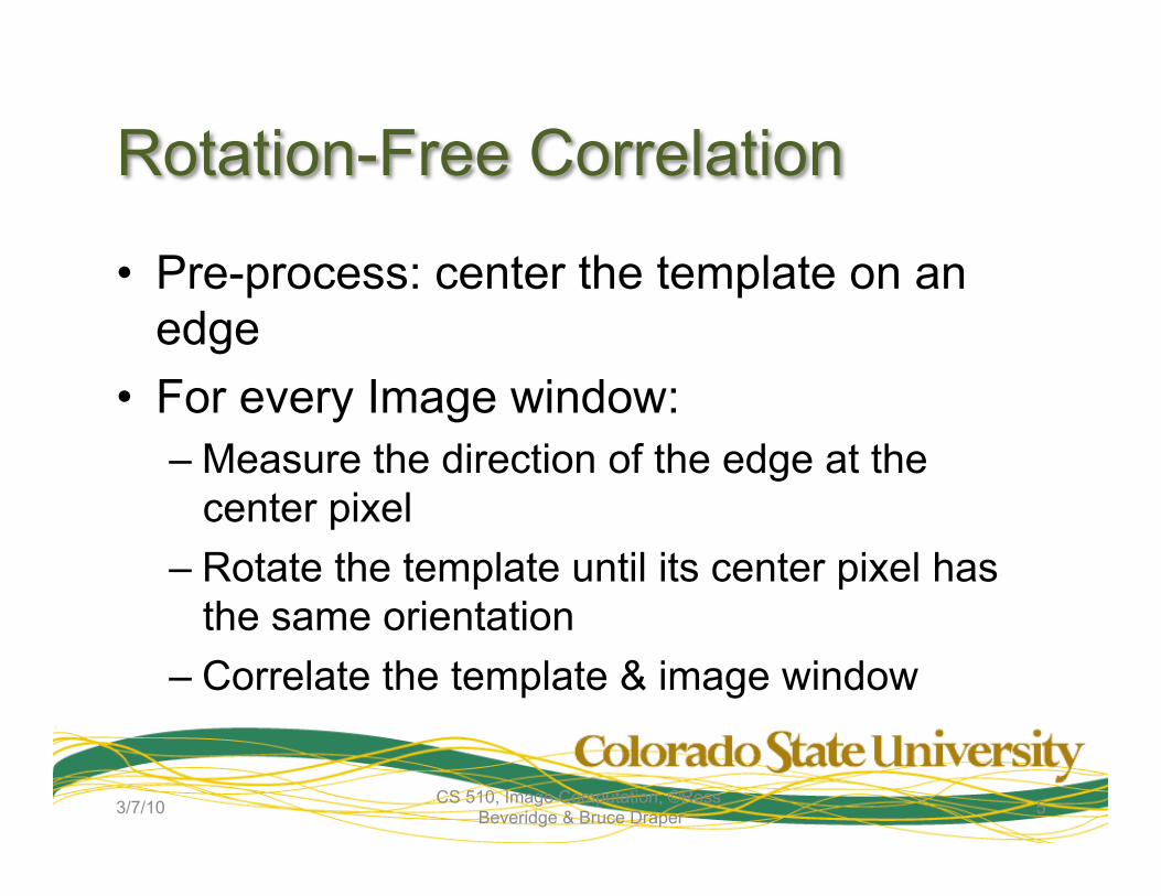
Rotation-Free Correlation
• Pre-process: center the template on an edge
• For every Image window: – Measure the direction of the edge at the
center pixel – Rotate the template until its center pixel has
the same orientation – Correlate the template & image window
3/7/10 CS 510, Image Computation, ©Ross Beveridge & Bruce Draper 5

Rotation-Free Correlation (II)
3/7/10 CS 510, Image Computation, ©Ross Beveridge & Bruce Draper 6
• Use different template orientation at every position • At least bilinear
interpolation • Skip positions with no
edge • i.e. mag ≈ 0

Problem: edge accuracy
• The orientation of an edge may not be accurate – Occlusion – Surface marking (smudge) – Electronic noise
• Solution: compute dominant edge orientation over a window
3/7/10 CS 510, Image Computation, ©Ross Beveridge & Bruce Draper 7

Example
dx
dy
2/18/13 8 CS 510, Image Computation, ©Ross Beveridge & Bruce Draper

Computing Edge Orientation Dominance • How do we determine the dominant
orientation from a set of [dx, dy] vectors? • Fit the line that best fits the (dx, dy) points • Represent edges as a matrix:
3/7/10 CS 510, Image Computation, ©Ross Beveridge & Bruce Draper 9
€
G =∂I∂x1
∂I∂x2
∂I∂xn
∂I∂y1
∂I∂y2
∂I∂yn
⎡
⎣
⎢ ⎢
⎤
⎦
⎥ ⎥

A general solution…
• Mean center the edge data
• Fit a line the minimizes the squared perpendicular distances
3/7/10 CS 510, Image Computation, ©Ross Beveridge & Bruce Draper 10
dx
dy

Edge Covariance
• Compute the outer product of G with itself:
• This matrix is called the structure tensor • What is the semantics of the structure
tensor?
3/7/10 CS 510, Image Computation, ©Ross Beveridge & Bruce Draper 11
€
Cov =GGT =dx1 dx2 dxndy1 dy2 dyn
⎡
⎣ ⎢
⎤
⎦ ⎥
dx1 dy1dx2 dy2 dxn dyn
⎡
⎣
⎢ ⎢ ⎢ ⎢
⎤
⎦
⎥ ⎥ ⎥ ⎥
=dxi
2
i∑ dxidyi
i∑
dxidyii∑ dyi
2
i∑
⎡
⎣
⎢ ⎢ ⎢
⎤
⎦
⎥ ⎥ ⎥
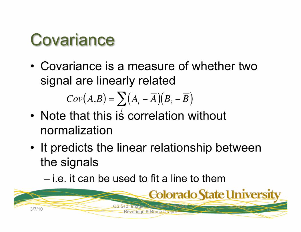
Covariance • Covariance is a measure of whether two
signal are linearly related
• Note that this is correlation without normalization
• It predicts the linear relationship between the signals – i.e. it can be used to fit a line to them
3/7/10 CS 510, Image Computation, ©Ross Beveridge & Bruce Draper 12
€
Cov A,B( ) = Ai − A ( )i∑ Bi − B ( )

Edge Covariance
• The structure tensor is the covariance matrix of the partial derivatives – It tells you the linear relation between the dx
and dy values – If all the orientations are the same, then dx
predicts dy (and vice versa) – If the orientations are random, dx has no
relation to dy.
3/7/10 CS 510, Image Computation, ©Ross Beveridge & Bruce Draper 13

Introduction to Principal Components Analysis (PCA) • We can solve the following:
• Where R is an orthonormal (rotation) matrix and λ is a diagonal matrix with descending values
• What do R and λ tell us?
3/7/10 CS 510, Image Computation, ©Ross Beveridge & Bruce Draper 14
€
GGT = R−1λR

Eigenvalues and Eigenvectors • R is a rotation matrix
– Its rows are axes of a new basis – The 1st row (eigenvector) is the best fit direction – The 2nd eigenvector is orthogonal to the 1st.
• λ contains the eigenvalues – The eigenvalues are the covariance in the
directions of the new bases • The closed form equation simply computed
the cosine of the first eigenvector
3/7/10 CS 510, Image Computation, ©Ross Beveridge & Bruce Draper 15

Corners (The Harris Operator) • The structure tensor is the outer product of
the partial derivatives with themselves:
• Consider the Eigenvalues – Both near zero => no edge – One large, one near zero => edge – Both large => a strong corner
2/18/13 CS 510, Image Computation, ©Ross Beveridge & Bruce Draper 16
€
C=dxi
2
i∑ dxidyi
i∑
dxidyii∑ dyi
2
i∑
⎡
⎣
⎢ ⎢ ⎢
⎤
⎦
⎥ ⎥ ⎥
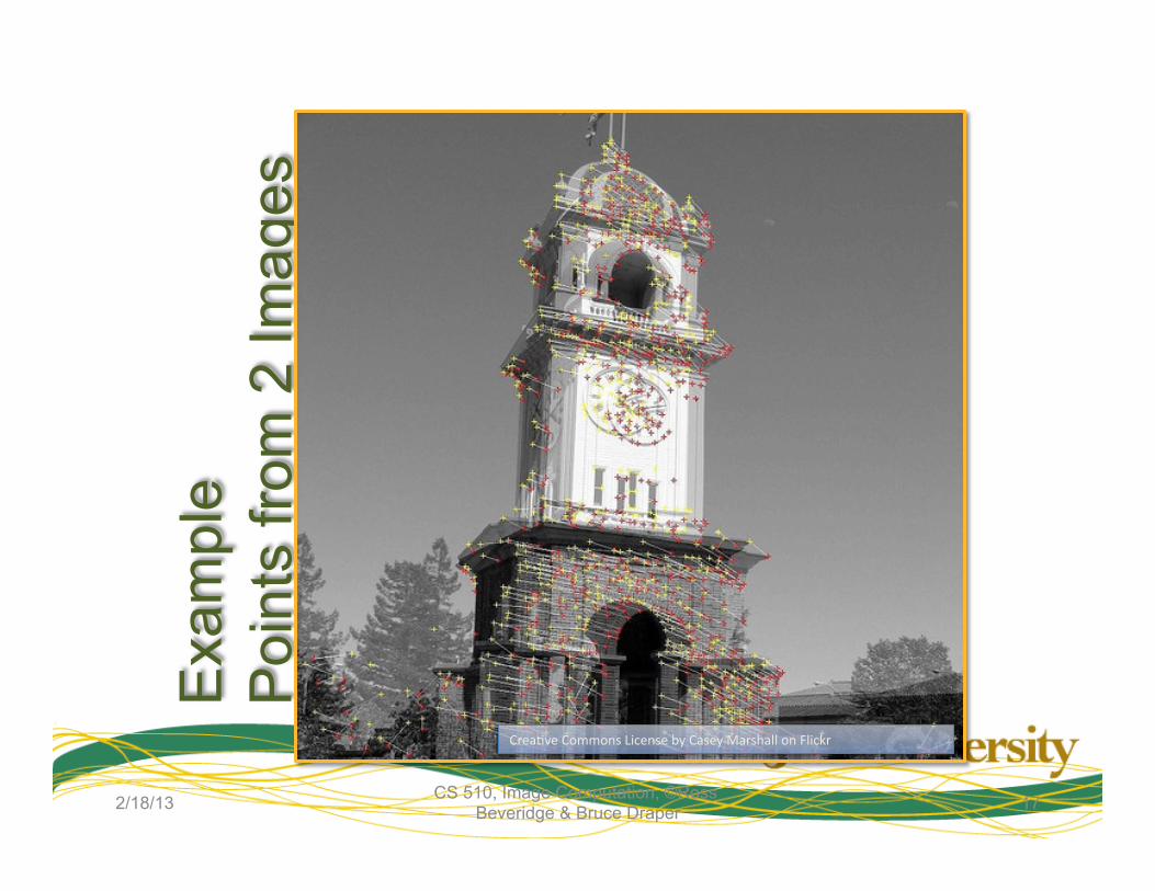
2/18/13 CS 510, Image Computation, ©Ross Beveridge & Bruce Draper 17
Exa
mpl
e P
oint
s fro
m 2
Imag
es
Crea%ve Commons License by Casey Marshall on Flickr

Back to Rotation-Free Correlation
• For every source window: – Calculate the edge
covariance matrix – Find the first
eigenvector – Rotate the template to
match – Correlate
3/7/10 CS 510, Image Computation, ©Ross Beveridge & Bruce Draper 18