An Intertemporal CAPM with Stochastic Volatility -...

An Intertemporal CAPM with StochasticVolatility

John Y. Campbell, Stefano Giglio, Christopher Polk, and Robert Turley1

First draft: October 2011This version: April 2014

1Campbell: Department of Economics, Littauer Center, Harvard University, Cambridge MA 02138, andNBER. Email [email protected]. Phone 617-496-6448. Giglio: Booth School of Business, Univer-sity of Chicago, 5807 S. Woodlawn Ave, Chicago IL 60637. Email [email protected]. Polk:Department of Finance, London School of Economics, London WC2A 2AE, UK. Email [email protected]: Baker Library 220D, Harvard Business School, Boston MA 02163. Email [email protected] are grateful to Torben Andersen, Gurdip Bakshi, John Cochrane, Bjorn Eraker, Bryan Kelly, Ian Martin,Sydney Ludvigson, Monika Piazzesi, Tuomo Vuolteenaho, and seminar participants at BI Norwegian Schoolof Management, CEMFI, the 2012 EFA, 2011 HBS Finance Unit research retreat, IESE, INSEAD, 2012Spring NBER Asset Pricing Meeting, Norges Bank Investment Management, Northwestern University, NYU,Oxford University, Stanford University, Swiss Finance Institute-Geneva, University of California-Berkeley,University of Chicago, University of Edinburgh, University of Illinois, University of Paris Dauphine, Univer-sity of Pennsylvania, and the 2012 WFA for comments. We thank Josh Coval, Ken French, Nick Roussanov,Mila Getmansky Sherman, and Tyler Shumway for providing data used in the analysis.

Abstract

This paper extends the approximate closed-form intertemporal capital asset pricing modelof Campbell (1993) to allow for stochastic volatility. The return on the aggregate stockmarket is modeled as one element of a vector autoregressive (VAR) system, and the volatilityof all shocks to the VAR is another element of the system. Our estimates of this VAR revealnovel low-frequency movements in market volatility tied to the default spread. We show thatgrowth stocks underperform value stocks because they hedge two types of deterioration ininvestment opportunities: declining expected stock returns, and increasing volatility. Ourmodel also prices portfolios of stocks sorted by risk exposures, and non-equity assets includingequity options, corporate bonds, and carry-trade currency portfolios.

JEL classi�cation: G12, N22

1 Introduction

The fundamental insight of intertemporal asset pricing theory is that long-term investorsshould care just as much about the returns they earn on their invested wealth as about thelevel of that wealth. In a simple model with a constant rate of return, for example, thesustainable level of consumption is the return on wealth multiplied by the level of wealth,and both terms in this product are equally important. In a more realistic model withtime-varying investment opportunities, conservative long-term investors will seek to hold�intertemporal hedges�, assets that perform well when investment opportunities deterio-rate. Such assets should deliver lower average returns in equilibrium if they are priced fromconservative long-term investors��rst-order conditions.

Since the seminal work of Merton (1973) on the intertemporal capital asset pricing model(ICAPM), a large empirical literature has explored the relevance of intertemporal considera-tions for the pricing of �nancial assets in general, and the cross-sectional pricing of stocks inparticular. One strand of this literature uses the approximate accounting identity of Camp-bell and Shiller (1988a) and the assumption that a representative investor has Epstein-Zinutility (Epstein and Zin 1989) to obtain approximate closed-form solutions for the ICAPM�srisk prices (Campbell 1993). These solutions can be implemented empirically if they arecombined with vector autoregressive (VAR) estimates of asset return dynamics (Campbell1996). Campbell and Vuolteenaho (2004), Campbell, Polk, and Vuolteenaho (2010), andCampbell, Giglio, and Polk (2013) use this approach to argue that value stocks outperformgrowth stocks on average because growth stocks do well when the expected return on theaggregate stock market declines; in other words, growth stocks have low risk premia becausethey are intertemporal hedges for long-term investors.

A weakness of the papers cited above is that they ignore time-variation in the volatility ofstock returns. In general, investment opportunities may deteriorate either because expectedstock returns decline or because the volatility of stock returns increases, and it is an empiricalquestion which of these two types of intertemporal risk have a greater e¤ect on asset returns.We address this weakness in this paper by extending the approximate closed-form ICAPM toallow for stochastic volatility. The resulting model explains risk premia in the stock marketusing three priced risk factors corresponding to three important attributes of aggregatemarket returns: revisions in expected future cash �ows, discount rates, and volatility. Anattractive feature of the model is that the prices of these three risk factors depend on onlyone free parameter, the long-horizon investor�s coe¢ cient of risk aversion.

Since the long-horizon investor in our model cares mostly about persistent changes inthe investment opportunity set, there must be predictable long-run variation in volatilityfor volatility risk to matter. Empirically, we implement our methodology using a vectorautoregression (VAR) including stock returns, realized variance, and other �nancial indica-tors that may be relevant for predicting returns and risk. Our VAR reveals low-frequencymovements in market volatility tied to the default spread, the yield spread of low-rated over

1

high-rated bonds. While this phenomenon has received little attention in the literature,we argue that it is sensible: Investors in risky bonds perceive the long-run component ofvolatility and incorporate this information when they set credit spreads, as risky bonds areshort the option to default over long maturities. Moreover, we show that GARCH-basedmethods that �lter only the information in past returns in order to disentangle the short-runand long-run volatility components miss this important low-frequency component.

With our novel model of long-run volatility in hand, we �nd that growth stocks have lowaverage returns because they outperform not only when the expected stock return declines,but also when stock market volatility increases. Thus growth stocks hedge two types ofdeterioration in investment opportunities, not just one. In the period since 1963 that createsthe greatest empirical di¢ culties for the standard CAPM, we �nd that the three-beta modelexplains over 62% of the cross-sectional variation in average returns of 25 portfolios sorted bysize and book-to-market ratios. The model is not rejected at the 5% level while the CAPMis strongly rejected. The implied coe¢ cient of relative risk aversion is an economicallyreasonable 6.9, in contrast to the much larger estimate of 20.7, which we get when weestimate a comparable version of the two-beta ICAPM of Campbell and Vuolteenaho (2004)using the same data.2 This success is due in large part to the inclusion of volatility betasin the speci�cation. The cross-sectional spread in volatility betas generates an annualizedaverage return spread of 5.2% compared to spreads of 2.8% and 2.2% for cash-�ow anddiscount-rate betas.

We con�rm that our �ndings are robust by looking at �ve alternative sets of test assets.First we sort stocks by their estimated risks, speci�cally their past market and volatilitybetas, and create risk-sorted portfolios. We do this to respond to the argument of Danieland Titman (1997, 2012) and Lewellen, Nagel, and Shanken (2010) that asset-pricing testsusing only portfolios sorted by characteristics known to be related to average returns, suchas size and value, can be misleading when the resulting portfolios have a low-dimensionalfactor structure. Second, we sort stocks by two characteristics� their book-market ratios andtheir idiosyncratic volatility� as well as their past volatility betas. This uncovers interestinginteractions among these characteristics and volatility betas, and allows us to address theidiosyncratic volatility e¤ect of Ang, Hodrick, Xing, and Zhang (2006), which is a majorchallenge to extant asset-pricing models. Third, we look at option and bond portfolios thatare exposed to aggregate volatility risk, speci�cally the S&P 100 index straddle of Covaland Shumway (2001) and the risky bond factor of Fama and French (1993), which shouldbe sensitive to changes in aggregate volatility since risky corporate debt is short the optionto default. Fourth, we look at currency portfolios sorted by interest rates in the manner ofLustig, Roussanov, and Verdelhan (2011), which capture the risk and return properties ofthe foreign exchange carry trade. Finally, we study variance forwards. These positions areexposed to realized volatility occurring from one to 12 months forward and thus present animportant check on the internal consistency of our model. In all these cases we �nd that ourthree-beta ICAPM, unlike the CAPM or the two-beta ICAPM, delivers satisfactory pricing

2The risk aversion estimate reported in Campbell and Vuolteenaho�s (2004) paper is 28.8.

2

results with minimal variation in parameters across test assets.

The organization of our paper is as follows. Section 2 reviews related literature. Section3 lays out the approximate closed-form ICAPM and extends it to incorporate stochasticvolatility. Section 4 presents data, econometrics, and VAR estimates of the dynamic processfor stock returns and realized volatility. This section documents the empirical success of ourmodel in forecasting long-run volatility. Section 5 introduces our test assets and estimatestheir betas with news about the market�s future cash �ows, discount rates, and volatility.Section 6 turns to cross-sectional asset pricing and estimates a representative investor�spreference parameters to �t a cross-section of test assets, taking the dynamics of stockreturns as given. Section 7 explores the implications of our model for the history of investors�marginal utility and consumption behavior. Section 8 presents a set of robustness exercisesin which we vary our basic VAR speci�cation for the dynamics of aggregate returns and risk,and explore the underlying components of volatility betas for the market portfolio and forvalue stocks versus growth stocks. Section 9 concludes. An online appendix to the paper(Campbell, Giglio, Polk, and Turley 2014) provides supporting details.

2 Literature Review

Our work is complementary to recent research on the �long-run risk model�of asset prices(Bansal and Yaron 2004) which can be traced back to insights in Kandel and Stambaugh(1991). Both the approximate closed-form ICAPM and the long-run risk model start withthe �rst-order conditions of an in�nitely lived Epstein-Zin representative investor. As orig-inally stated by Epstein and Zin (1989), these �rst-order conditions involve both aggregateconsumption growth and the return on the market portfolio of aggregate wealth. Campbell(1993) pointed out that the intertemporal budget constraint could be used to substituteout consumption growth, turning the model into a Merton-style ICAPM. Restoy and Weil(1998, 2011) used the same logic to substitute out the market portfolio return, turning themodel into a generalized consumption CAPM in the style of Breeden (1979).

Kandel and Stambaugh (1991) were the �rst researchers to study the implications forasset returns of time-varying �rst and second moments of consumption growth in a modelwith a representative Epstein-Zin investor. Speci�cally, Kandel and Stambaugh (1991) as-sumed a four-state Markov chain for the expected growth rate and conditional volatilityof consumption, and provided closed-form solutions for important asset-pricing moments.In the same spirit Bansal and Yaron (2004) added stochastic volatility to the Restoy-Weilmodel, and subsequent theoretical and empirical research in the long-run risk framework hasincreasingly emphasized the importance of stochastic volatility (Bansal, Kiku, and Yaron2012, Beeler and Campbell 2012, Hansen 2012). In this paper we give the approximateclosed-form ICAPM the same capability to handle stochastic volatility that its cousin, thelong-run risk model, already possesses.

3

One might ask whether there is any reason to work with an ICAPM rather than aconsumption-based model given that these are two representations of the same underlyingeconomic structure. Writing the model as an ICAPM is conceptually appealing becauseit describes risks as they appear to an investor who takes asset prices as given and choosesconsumption to satisfy his budget constraint. This is a valuable microeconomic complementto the macroeconomic perspective provided by the consumption-based approach.

The ICAPM also has several advantages as an empirical speci�cation. First, it doesnot require that all agents in the economy participate in �nancial markets. So long as anagent with Epstein-Zin preferences holds the aggregate wealth portfolio, the ICAPM willhold even if there are other agents in the economy who receive non�nancial income andaccount for some portion of aggregate consumption.3 Related to this, the ICAPM can begiven a microeconomic interpretation as a description of the conditions that are required fora long-term equity investor not to tilt his portfolio towards stocks with high average returnssuch as value stocks. We discuss this interpretation brie�y in the conclusion of the paper.

Second, the ICAPM allows an empirical analysis based on �nancial proxies for the ag-gregate market portfolio rather than on accurate measurement of aggregate consumption.While there are certainly challenges to the accurate measurement of �nancial wealth, �nan-cial time series are generally available on a more timely basis and over longer sample periodsthan consumption series. Our analysis follows a large literature that assumes that the returnon a broad stock index is a reasonable proxy for the return on aggregate wealth. In therobustness section, we explore the sensitivity of our results to using other proxies for thewealth portfolio.

Third, the ICAPM generates empirical predictions that depend on the coe¢ cient of rel-ative risk aversion but not the elasticity of intertemporal substitution. This means thatwe do not need to assume a wedge between risk aversion and the reciprocal of the elastic-ity of intertemporal substitution, and therefore do not face the critique of Epstein, Farhi,and Strzalecki (2013) that a large wedge implies an unrealistic willingness to pay for earlyresolution of uncertainty.4

The particular speci�cation of the ICAPM in this paper has two further advantages. It is�exible enough to allow multiple state variables that can be estimated in a VAR system, so itdoes not require low-dimensional calibration of the sort used in the long-run risk literature.And we use an a¢ ne stochastic volatility process that governs the volatility of all statevariables, including itself. We show that this assumption �ts �nancial data reasonably well,and it guarantees that stochastic volatility would always remain positive in a continuous-

3Hansen (2014) highlights this point in his Nobel Lecture. Malloy, Moskowitz, and Vissing-Jørgensen(2009) study long-run consumption risk using microeconomic data on stockholders� consumption growth,but they can only do this over a relatively short sample period.

4We use the standard terminology to describe the two parameters of the Epstein-Zin utility function, asrisk aversion and as the elasticity of intertemporal substitution, although Garcia, Renault, and Semenov(2006) and Hansen, Heaton, Lee, and Roussanov (2007) point out that this interpretation may not be correctwhen di¤ers from the reciprocal of .

4

time version of the model, a property that does not always hold in current implementationsof the long-run risk model.5

The closest precursors to our work are unpublished papers by Chen (2003) and Sohn(2010). Both papers explore the e¤ects of stochastic volatility on asset prices in an ICAPMsetting but make strong assumptions about the covariance structure of various news termswhen deriving their pricing equations. Chen (2003) assumes constant covariances betweenshocks to the market return (and powers of those shocks) and news about future expectedmarket return variance. Sohn (2010) makes two strong assumptions about asset returns andconsumption growth, speci�cally that all assets have zero covariance with news about futureconsumption growth volatility and that the conditional contemporaneous correlation betweenthe market return and consumption growth is constant through time. Du¤ee (2005) presentsevidence against the latter assumption. It is in any case unattractive to make assumptionsabout consumption growth in an ICAPM that does not require accurate measurement ofconsumption.

Chen estimates a VAR with a GARCH model to allow for time variation in the volatilityof return shocks, restricting market volatility to depend only on its past realizations and notthose of the other state variables. His empirical analysis has little success in explaining thecross-section of stock returns. Sohn uses a similar but more sophisticated GARCH modelfor market volatility and tests how well short-run and long-run risk components from theGARCH estimation can explain the returns of various stock portfolios, comparing the resultsto factors previously shown to be empirically successful. In contrast, our paper incorporatesthe volatility process directly in the ICAPM, allowing heteroskedasticity to a¤ect and tobe predicted by all state variables, and showing how the price of volatility risk is pinneddown by the time-series structure of the model along with the investor�s coe¢ cient of riskaversion.

Bansal, Kiku, Shaliastovich and Yaron (2013), a paper contemporaneous with ours, ex-plores the e¤ects of stochastic volatility in the long-run risk model. Like us, they �ndstochastic volatility to be an important feature in the time series of equity returns. Thereare some important di¤erences in the underlying models. In particular, in their benchmarkmodel they assume that the stochastic process driving volatility is homoskedastic. In our the-oretical analysis we discuss some conditions that are required for their model solution to bevalid, and argue that these conditions are not satis�ed empirically. The di¤erent modelingassumptions and some di¤erences in empirical implementation account for our contrastingempirical results; we show that volatility risk is very important in explaining the cross-sectionof stock returns while they �nd it has little impact on cross-sectional di¤erences in risk pre-mia. Indeed, Bansal, Kiku, Shaliastovich and Yaron (2013) �nd that a value-minus-growthbet has a positive beta with volatility news, while we �nd it always has a negative volatility

5Eraker (2008), Eraker and Shaliastovich (2008), and Heaton (2012) are exceptions whose models doguarantee positive volatility. A¢ ne stochastic volatility models date back at least to Heston (1993) incontinuous time, and have been developed and discussed by Ghysels, Harvey, and Renault (1996), Meddahiand Renault (2004), and Darolles, Gourieroux, and Jasiak (2006) among others.

5

beta. Our negative volatility beta estimate is more consistent with models of real optionsheld by growth �rms, such as McQuade (2012), and with the underperformance of valuestocks during periods of elevated volatility including the Great Depression, the technologyboom of the late 1990s, and the Great Recession of the late 2000s (Campbell, Giglio, andPolk 2013).

Stochastic volatility has been explored in other branches of the �nance literature. Forexample, Chacko and Viceira (2005) and Liu (2007) show how stochastic volatility a¤ects theoptimal portfolio choice of long-term investors. Chacko and Viceira assume an AR(1) processfor volatility and argue that movements in volatility are not persistent enough to generatelarge intertemporal hedging demands. Our more �exible multivariate process does allowus to detect persistent long-run variation in volatility. Campbell and Hentschel (1992),Calvet and Fisher (2007), and Eraker and Wang (2011) argue that volatility shocks willlower aggregate stock prices by increasing expected returns, if they do not a¤ect cash �ows.The strength of this volatility feedback e¤ect depends on the persistence of the volatilityprocess. Coval and Shumway (2001), Ang, Hodrick, Xing, and Zhang (2006), and Adrianand Rosenberg (2008) present evidence that shocks to market volatility are priced risk factorsin the cross-section of stock returns, but they do not develop any theory to explain the riskprices for these factors.

Time-varying volatility is a prime concern of the �eld of �nancial econometrics. SinceEngle�s (1982) seminal paper on ARCH, much of the �nancial econometrics literature hasfocused on variants of the univariate GARCH model (Bollerslev 1986), in which returnvolatility is modeled as a function of past shocks to returns and of its own lags (see Poonand Granger (2003) and Andersen et al. (2006) for recent surveys). More recently, realizedvolatility from high-frequency data has been used to estimate stochastic volatility processes(Barndor¤-Nielsen and Shephard 2002, Andersen et al. 2003). The use of realized volatilityhas improved the modeling and forecasting of volatility, including its long-run component;however, this literature has primarily focused on the information content of high-frequencyintra-daily return data. This allows very precise measurement of volatility, but at the sametime, given data availability constraints, limits the potential to use long time series to learnabout long-run movements in volatility. In our paper, we measure realized volatility onlywith daily data, but augment this information with other �nancial time series that revealinformation investors have about underlying volatility components.

A much smaller literature has, like us, looked directly at the information in other variablesconcerning future volatility. In early work, Schwert (1989) links movements in stock marketvolatility to various indicators of economic activity, particularly the price-earnings ratioand the default spread, but �nds relatively weak connections. Engle, Ghysels and Sohn(2013) study the e¤ect of in�ation and industrial production growth on volatility, �ndinga signi�cant link between the two, especially at long horizons. Campbell and Taksler(2003) look at the cross-sectional link between corporate bond yields and equity volatility,emphasizing that bond yields respond to idiosyncratic �rm-level volatility as well as aggregatevolatility. Two recent papers, Paye (2012) and Christiansen et al. (2012), look at larger

6

sets of potential volatility predictors, including the default spread and valuation ratios, to�nd those that have predictive power for quarterly realized variance. The former paper,in a standard regression framework, �nds that the commercial paper to Treasury spreadand the default spread, among other variables, contain useful information for predictingvolatility. The latter uses Bayesian Model Averaging to �nd the most successful predictors,and documents the importance of the default spread and valuation ratios in forecastingshort-run volatility.

Finally, our paper relates to the enormous literature on cross-sectional patterns in stockreturns. Most obviously, we contribute to the longstanding debate on the explanationof the value e¤ect. Beyond this, our alternative test assets allow us to make two othercontributions. By sorting stocks on their estimated market and volatility betas, we showthat in the period since 1963, stocks with high past market betas tend to have high futurevolatility betas, a desirable property which reduces their equilibrium returns and may help toexplain the weak relation between past market betas and returns (Fama and French 1992).Also, by sorting stocks on book-market ratios, idiosyncratic volatility, and past volatilitybetas, we show that idiosyncratic volatility is associated with higher volatility betas amonggrowth stocks but much less so among value stocks. This is consistent with the intuitionthat idiosyncratic volatility reveals the presence of growth options among growth stocks,and it may also help to explain the �nding of Ang, Hodrick, Xing, and Zhang (2006) thatidiosyncratic volatility is negatively associated with average returns.6

3 An Intertemporal Model with Stochastic Volatility

3.1 Asset pricing with time varying risk

Preferences

We begin by assuming a representative agent with Epstein-Zin preferences. We writethe value function as

Vt =h(1� �)C

1� �

t + ��Et�V 1� t+1

��1=�i �1�

; (1)

where Ct is consumption and the preference parameters are the discount factor �; risk aversion

6Ang, Hodrick, Xing, and Zhang (2006) argue that the idiosyncratic volatility e¤ect cannot be explainedby aggregate volatility risk while Barinov (2013) and Chen and Petkova (2014) argue that it can. None ofthese papers develop a fully-�eshed-out theory to motivate their speci�c volatility risk factor or explain therisk price of that factor. The idiosyncratic volatility e¤ect is non-monotonic as documented in Table VIof Ang, Hodrick, Xing, and Zhang (2006), and it varies across samples and methodologies as documentedby Bali and Cakici (2009) and Fu (2009), possibly re�ecting the interaction with the book-market ratiodocumented here.

7

, and the elasticity of intertemporal substitution . For convenience, we de�ne � =(1� )=(1� 1= ).

The corresponding stochastic discount factor (SDF) can be written as

Mt+1 =

�

�CtCt+1

�1= !� �Wt � CtWt+1

�1��; (2)

where Wt is the market value of the consumption stream owned by the agent, includingcurrent consumption Ct.7 The log return on wealth is rt+1 = ln (Wt+1= (Wt � Ct)), the logvalue of wealth tomorrow divided by reinvested wealth today. The log SDF is therefore

mt+1 = � ln � � �

�ct+1 + (� � 1) rt+1: (3)

A convenient identity

The gross return to wealth can be written

1 +Rt+1 =Wt+1

Wt � Ct=

�Ct

Wt � Ct

��Ct+1Ct

��Wt+1

Ct+1

�; (4)

expressing it as the product of the current consumption payout, the growth in consumption,and the future price of a unit of consumption.

We �nd it convenient to work in logs. We de�ne the log value of reinvested wealth perunit of consumption as zt = ln ((Wt � Ct) =Ct), and the future value of a consumption claimas ht+1 = ln (Wt+1=Ct+1), so that the log return is:

rt+1 = �zt +�ct+1 + ht+1: (5)

Heuristically, the return on wealth is negatively related to the current value of reinvestedwealth and positively related to consumption growth and the future value of wealth. Thelast term in equation (5) will capture the e¤ects of intertemporal hedging on asset prices,hence the choice of the notation ht+1 for this term.

The ICAPM

We assume that asset returns are jointly conditionally lognormal, but we allow changingconditional volatility so we are careful to write second moments with time subscripts toindicate that they can vary over time. Under this standard assumption, the expected returnon any asset must satisfy

0 = lnEt expfmt+1 + ri;t+1g = Et [mt+1 + ri;t+1] +1

2Vart [mt+1 + ri;t+1] ; (6)

7This notational convention is not consistent in the literature. Some authors exclude current consumptionfrom the de�nition of current wealth.

8

and the risk premium on any asset is given by

Etri;t+1 � rf;t +1

2Vartrt+1 = �Covt [mt+1; ri;t+1] : (7)

The convenient identity (5) can be used to write the log SDF (3) without reference toconsumption growth:

mt+1 = � ln � � �

zt +

�

ht+1 � rt+1: (8)

Since the �rst two terms in (5) are known at time t, only the latter two terms appear in theconditional covariance in (7). We obtain an ICAPM pricing equation that relates the riskpremium on any asset to the asset�s covariance with the wealth return and with shocks tofuture consumption claim values:


2Vartrt+1 = Covt [ri;t+1; rt+1]�

�

Covt [ri;t+1; ht+1] (9)

Return and risk shocks in the ICAPM

To better understand the intertemporal hedging component ht+1, we proceed in two steps.First, we approximate the relationship of ht+1 and zt+1 by taking a loglinear approximationabout �z:

ht+1 � �+ �zt+1 (10)

where the loglinearization parameter � = exp(�z)=(1 + exp(�z)) � 1� C=W .

Second, we apply the general pricing equation (6) to the wealth portfolio itself (settingri;t+1 = rt+1), and use the convenient identity (5) to substitute out consumption growth fromthis expression. Rearranging, we can write the variable zt as

zt = ln � + ( � 1)Etrt+1 + Etht+1 +

�

1

2Vart [mt+1 + rt+1] : (11)

Third, we combine these expressions to obtain the innovation in ht+1:

ht+1 � Etht+1 = �(zt+1 � Etzt+1)

= (Et+1 � Et)��( � 1)rt+2 + ht+2 +

�

1

2Vart+1 [mt+2 + rt+2]

�: (12)

Solving forward to an in�nite horizon,

ht+1 � Etht+1 = ( � 1)(Et+1 � Et)1Xj=1

�jrt+1+j

+1

2

�(Et+1 � Et)

1Xj=1

�jVart+j [mt+1+j + rt+1+j]

= ( � 1)NDR;t+1 +1

2

�NRISK;t+1: (13)

9

The second equality follows Campbell and Vuolteenaho (2004) and uses the notation NDR

(�news about discount rates�) for revisions in expected future returns. In a similar spiritwe write revisions in expectations of future risk (the variance of the future log return plusthe log stochastic discount factor) as NRISK .

Finally, we substitute back into the intertemporal model (9):


2Vartri;t+1

= Covt [ri;t+1; rt+1] + ( � 1)Covt [ri;t+1; NDR;t+1]�1

2Covt [ri;t+1; NRISK;t+1]

= Covt [ri;t+1; NCF;t+1] + Covt [ri;t+1;�NDR;t+1]�1

2Covt [ri;t+1; NRISK;t+1] : (14)

The �rst equality expresses the risk premium as risk aversion times covariance with thecurrent market return, plus ( �1) times covariance with news about future market returns,minus one half covariance with risk. This is an extension of the ICAPM as written byCampbell (1993), with no reference to consumption or the elasticity of intertemporal substi-tution :8 When the investor�s risk aversion is greater than 1, assets which hedge aggregatediscount rates (Covt [ri;t+1; NDR;t+1] < 0) or aggregate risk (Covt [ri;t+1; NRISK;t+1] > 0) havelower expected returns, all else equal.

The second equality rewrites the model, following Campbell and Vuolteenaho (2004), bybreaking the market return into cash-�ow news and discount-rate news. Cash-�ow newsNCF is de�ned by NCF = rt+1�Etrt+1+NDR. The price of risk for cash-�ow news is timesgreater than the price of risk for discount-rate news, hence Campbell and Vuolteenaho callbetas with cash-�ow news �bad betas�and those with discount-rate news �good betas�. Thethird term in (14) shows the risk premium associated with exposure to news about future risksand did not appear in Campbell and Vuolteenaho�s model, which assumed homoskedasticity.Not surprisingly, the coe¢ cient is negative, indicating that an asset providing positive returnswhen risk expectations increase will o¤er a lower return on average.

While the elasticity of intertemporal substitution does not a¤ect risk premia in ourmodel, this parameter does in�uence the implied behavior of the investor�s consumption.We explore this further in the online appendix to the paper.

3.2 From risk to volatility

The risk shocks de�ned in the previous subsection are shocks to the conditional volatility ofreturns plus the stochastic discount factor, and therefore are not directly observable. We

8Campbell (1993) brie�y considers the heteroskedastic case, noting that when = 1, Vart [mt+1 + rt+1]is a constant. This implies that NRISK does not vary over time so the stochastic volatility term disappears.Campbell claims that the stochastic volatility term also disappears when = 1, but this is incorrect. Whenlimits are taken correctly, NRISK does not depend on (except indirectly through the loglinearizationparameter, �).

10

now make additional assumptions on the data generating process for stock returns that allowus to estimate the news terms. These assumptions imply that the conditional volatility ofreturns plus the stochastic discount factor is proportional to the conditional volatility ofreturns themselves.

Suppose the economy is described by a �rst-order VAR

xt+1 = �x+ � (xt � �x) + �tut+1; (15)

where xt+1 is an n� 1 vector of state variables that has rt+1 as its �rst element, �2t+1 as itssecond element, and n�2 other variables that help to predict the �rst and second moments ofaggregate returns. �x and � are an n� 1 vector and an n�n matrix of constant parameters,and ut+1 is a vector of shocks to the state variables normalized so that its �rst elementhas unit variance. We assume that ut+1 has a constant variance-covariance matrix �, withelement �11 = 1.

The key assumption here is that a scalar random variable, �2t , equal to the conditionalvariance of market returns, also governs time-variation in the variance of all shocks to thissystem. Both market returns and state variables, including volatility itself, have innovationswhose variances move in proportion to one another. This assumption makes the stochasticvolatility process a¢ ne, as in Heston (1993) and related work discussed above in our literaturereview.

Given this structure, news about discount rates can be written as

NDR;t+1 = (Et+1 � Et)1Xj=1

�jrt+1+j

= e01

1Xj=1

�j�j�tut+1

= e01�� (I� ��)�1 �tut+1; (16)

while implied cash �ow news is:

NCF;t+1 = (rt+1 � Etrt+1) +NDR;t+1

=�e01 + e

01��(I� ��)�1

��tut+1: (17)

Furthermore, our log-linear model will make the log SDF, mt+1; a linear function of thestate variables. Since all shocks to the SDF are then proportional to �t, Vart [mt+1 + rt+1] /�2t : As a result, the conditional variance, Vart [(mt+1 + rt+1) =�t] = !t, will be a constantthat does not depend on the state variables. Without knowing the parameters of the utilityfunction, we can write Vart [mt+1 + rt+1] = !�2t so that the news about risk, NRISK , is

11

proportional to news about market return variance, NV .

NRISK;t+1 = (Et+1 � Et)1Xj=1

�jVart+j [rt+1+j +mt+1+j]

= (Et+1 � Et)1Xj=1

�j�!�2t+j

�= !�e02

1Xj=0

�j�j�tut+1

= !�e02 (I� ��)�1 �tut+1 = !NV;t+1: (18)

Substituting (18) into (14), we obtain an empirically-testable intertemporal CAPM withstochastic volatility:


2Vartri;t+1

= Covt [ri;t+1; NCF;t+1] + Covt [ri;t+1;�NDR;t+1]�1

2!Covt [ri;t+1; NV;t+1] , (19)

where covariances with news about three key attributes of the market portfolio (cash �ows,discount rates, and volatility) describe the cross section of average returns.

The parameter ! is a nonlinear function of the coe¢ cient of relative risk aversion , aswell as the VAR parameters and the loglinearization coe¢ cient �, but it does not depend onthe elasticity of intertemporal substitution except indirectly through the in�uence of on�. In the online appendix, we show that ! solves:

!�2t = (1� )2Vart�NCFt+1

�+ !(1� )Covt

�NCFt+1;NVt+1;

�+ !2

1

4Vart

�NVt+1

�: (20)

We can see two main channels through which a¤ects !. First, a higher risk aversion�given the underlying volatilities of all shocks� implies a more volatile stochastic discountfactor m, and therefore a higher RISK. This e¤ect is proportional to (1 � )2, so it in-creases rapidly with . Second, there is a feedback e¤ect on RISK through future risk: !appears on the right-hand side of the equation as well. Given that in our estimation we �ndCovt

�NCFt+1;NVt+1;

�< 0, this second e¤ect makes ! increase even faster with .9

9Bansal, Kiku, Shaliastovich and Yaron (2013) derive a similar expression, equation (16) in their paper.They claim that the equivalent expression for ! in their model reduces to (1� )2 in the case of homoskedasticvolatility (their equation 17). We discuss the conditions required for their claim to be valid in the nextsubsection. In a robustness test, they also derive a corresponding equation for the case of time-varyingvolatility (their equation C.4), but proceed with a linearization procedure that, as we discuss below, allowsthe parameters of the model to lie in a region of the parameter space where the true model does not have asolution.

12

This equation can also be written directly in terms of the VAR parameters. We de�nexCF and xV as the error-to-news vectors that map VAR innovations to volatility-scaled newsterms:

1

�tNCF;t+1 = xCFut+1 =

�e01 + e

01��(I� ��)�1

�ut+1 (21)

1

�tNV;t+1 = xV ut+1 =

�e02�(I� ��)�1

�ut+1: (22)

Then ! solves

0 = !21

4xV�x

0V � ! (1� (1� )xCF�x

0V ) + (1� )2 xCF�x

0CF (23)

This quadratic equation for ! has two solutions, but the online appendix shows that oneof the solutions can be disregarded. This false solution is easily identi�ed by its implicationthat ! becomes in�nite as volatility shocks become small. The correct solution is

! =1� (1� )xCF�x

0V �

p(1� (1� )xCF�x

0V )2 � (1� )2(xV�x

0V )(xCF�x

0CF )

12xV�x

0V

(24)

3.3 Conditions for the existence of a solution

Equation (23) has a real solution only if

(1� (1� )xCF�x0V )2 � (1� )2(xV�x

0V )(xCF�x

0CF ) � 0. (25)

Otherwise, if risk aversion, volatility shocks and cash �ow shocks are large enough, as mea-sured by the product (1 � )2(xV�x

0V )(xCF�x

0CF ), equation (23) may deliver a complex

rather than a real value for !. Given our VAR estimates of the variance and covarianceterms, we �nd a real solution for ! as ranges from zero to 6:9. Figure 1 plots ! as afunction of based on these estimates.

The online appendix shows that the condition for the existence of a real solution can bewritten in a simpler form as

(�n � 1)(1� )�cf�v � 1; (26)

where �n is the correlation between the news termsNCF andNV , �cf is the standard deviationof the scaled news NCF;t+1=�t, and �v is the standard deviation of the scaled news NV;t+1=�t.

To further develop the intuition behind these equations, in the online appendix we studya simple example in which the link between the existence to a solution for equation (23)and the existence of a value function for the representative agent can be shown analytically.

13

We do this in the special case of = 1, since we can then solve directly for the valuefunction without any need for a loglinear approximation of the return on the wealth portfolio(Tallarini 2000, Hansen, Heaton, and Li 2008). In the example we �nd that the conditionfor the existence of the value function coincides precisely with the condition for the existenceof a real solution to the quadratic equation for !, equation (25). This result indicates thatthe possible non-existence of a solution to the quadratic equation for ! is a deep featureof the model, not an artefact of our loglinear approximation� which is not needed in thespecial case where = 1. We also show that the problem arises because the value functionbecomes ever more sensitive to volatility as the volatility of the value function increases,and this sensitivity feeds back into the volatility of the value function, further increasing it.When this positive feedback becomes too powerful, then the value function ceases to exist.

This constraint on the parameters of the model is ignored in Bansal, Kiku, Shaliastovich,and Yaron (BKSY 2013), when they consider the case of time-varying volatility of volatilityas a robustness test in Sections II.E and III.D. There, rather than imposing that ! and satisfy equation (23), they proceed to linearize equation (23) so that a solution for omegaexists for all values of gamma. Therefore, they allow combinations of ( ,!) for which equation(23) doesn�t admit a real solution �in which case, as we show in the appendix, the true modeldoesn�t have a solution.10

The online appendix also considers the benchmark speci�cation of BKSY in which thevolatility process is homoskedastic. In this case the term Vart(mt+1+ rt+1) is not in generalproportional to �2t , but depends on both �

2t and �t. Therefore, NRISK (news about future

values of Vart(mt+1 + rt+1)) is not in general proportional to NV , so that NV is not ingeneral the right news term to use in cross-sectional pricing. The appendix shows thatproportionality of NRISK and NV in the homoskedastic case can only be obtained withadditional special assumptions not stated by BKSY: that NCF and NV are uncorrelated,and that the NV shock only depends on innovations of state variables which are themselveshomoskedastic. As both of these assumptions are strongly rejected by the data, we do notfurther consider the model with homoskedastic �2t .

In summary, this section has shown that in our model, the existence of a real solutionfor ! is tightly linked with the existence of the value function. As a consequence, in ourempirical analysis we take seriously the constraint implied by the quadratic equation (23),and require that our parameter estimates satisfy this constraint. Given the high averagereturns to risky assets in historical data, this means in practice that our estimate of riskaversion is often equal to the estimated upper bound of 6.9.

10In a previous version of our paper, we used also used this linearization to solve equation (23). For thereasons explained above, we now instead require the non-linearized quadratic equation (23) to have a realsolution.

14

4 Predicting Aggregate Stock Returns and Volatility

4.1 State variables

Our full VAR speci�cation of the vector xt+1 includes six state variables, �ve of which arethe same as in Campbell, Giglio and Polk (2011). To those �ve variables, we add an estimateof conditional volatility. The data are all quarterly, from 1926:2 to 2011:4.

The �rst variable in the VAR is the log real return on the market, rM , the di¤erencebetween the log return on the Center for Research in Securities Prices (CRSP) value-weightedstock index and the log return on the Consumer Price Index. This is a standard proxy forthe aggregate wealth portfolio, but in the robustness section we consider alternative proxiesthat delever the market return by combining it in various proportions with Treasury bills.

The second variable is expected market variance (EV AR). This variable is meant tocapture the variance of market returns, �2t , conditional on information available at timet, so that innovations to this variable can be mapped to the NV term described above.To construct EV ARt, we proceed as follows. We �rst construct a series of within-quarterrealized variance of daily returns for each time t, RV ARt. We then run a regression ofRV ARt+1 on lagged realized variance (RV ARt) as well as the other �ve state variables attime t. This regression then generates a series of predicted values for RV AR at each timet + 1, that depend on information available at time t: dRV ARt+1. Finally, we de�ne ourexpected variance at time t to be exactly this predicted value at t+ 1:

EV ARt � dRV ARt+1:

Note that though we describe our methodology in a two-step fashion where we �rst estimateEV AR and then use EV AR in a VAR, this is only for interpretability. Indeed, this approachto modelingEV AR can be considered a simple renormalization of equivalent results we would�nd from a VAR that included RV AR directly.11

The third variable is the price-earnings ratio (PE) from Shiller (2000), constructed asthe price of the S&P 500 index divided by a ten-year trailing moving average of aggregateearnings of companies in the S&P 500 index. Following Graham and Dodd (1934), Campbelland Shiller (1988b, 1998) advocate averaging earnings over several years to avoid temporaryspikes in the price-earnings ratio caused by cyclical declines in earnings. We avoid anyinterpolation of earnings as well as lag the moving average by one quarter in order to ensurethat all components of the time-t price-earnings ratio are contemporaneously observable bytime t. The ratio is log transformed.

11Since we weight observations based on RV AR in the �rst stage and then reweight observations usingEV AR in the second stage, our two-stage approach in practice is not exactly the same as a one-stageapproach. However, Panel B of Table 11 shows that results from a RV AR-weighted single-step estimationare qualitatively very similar to those produced by our two-stage approach.

15

Fourth, the term yield spread (TY ) is obtained from Global Financial Data. We computethe TY series as the di¤erence between the log yield on the 10-Year US Constant MaturityBond (IGUSA10D) and the log yield on the 3-Month US Treasury Bill (ITUSA3D).

Fifth, the small-stock value spread (V S) is constructed from data on the six �elementary�equity portfolios also obtained from Professor French�s website. These elementary portfolios,which are constructed at the end of each June, are the intersections of two portfolios formedon size (market equity, ME) and three portfolios formed on the ratio of book equity to marketequity (BE/ME). The size breakpoint for year t is the median NYSE market equity at theend of June of year t. BE/ME for June of year t is the book equity for the last �scal yearend in t � 1 divided by ME for December of t � 1. The BE/ME breakpoints are the 30thand 70th NYSE percentiles.

At the end of June of year t, we construct the small-stock value spread as the di¤erencebetween the ln(BE=ME) of the small high-book-to-market portfolio and the ln(BE=ME)of the small low-book-to-market portfolio, where BE and ME are measured at the end ofDecember of year t � 1. For months from July to May, the small-stock value spread isconstructed by adding the cumulative log return (from the previous June) on the small low-book-to-market portfolio to, and subtracting the cumulative log return on the small high-book-to-market portfolio from, the end-of-June small-stock value spread. The constructionof this series follows Campbell and Vuolteenaho (2004) closely.

The sixth variable in our VAR is the default spread (DEF ), de�ned as the di¤erencebetween the log yield on Moody�s BAA and AAA bonds. The series is obtained from theFederal Reserve Bank of St. Louis. Campbell, Giglio and Polk (2011) add the default spreadto the Campbell and Vuolteenaho (2004) VAR speci�cation in part because that variable isknown to track time-series variation in expected real returns on the market portfolio (Famaand French, 1989), but mostly because shocks to the default spread should to some degreere�ect news about aggregate default probabilities. Of course, news about aggregate defaultprobabilities should in turn re�ect news about the market�s future cash �ows and volatility.

4.2 Short-run volatility estimation

In order for the regression model that generates EV ARt to be consistent with a reasonabledata-generating process for market variance, we deviate from standard OLS in two ways.First, we constrain the regression coe¢ cients to produce �tted values (i.e. expected marketreturn variance) that are positive. Second, given that we explicitly consider heteroskedas-ticity of the innovations to our variables, we estimate this regression using Weighted LeastSquares (WLS), where the weight of each observation pair (RV ARt+1, xt) is initially basedon the time-t value of (RV AR)�1. However, to ensure that the ratio of weights across obser-vations is not extreme, we shrink these initial weights towards equal weights. In particular,we set our shrinkage factor large enough so that the ratio of the largest observation weight

16

to the smallest observation weight is always less than or equal to �ve. Though admittedlysomewhat ad hoc, this bound is consistent with reasonable priors of the degree of variationover time in expected market return variance. More importantly, we show later (in Table 12Panel B) that our results are robust to variation in this bound. Both the constraint on theregression�s �tted values and the constraint on WLS observation weights bind in the samplewe study.

The results of the �rst stage regression generating the state variable EV ARt are reportedin Table 1 Panel A. Perhaps not surprisingly, past realized variance strongly predicts futurerealized variance. More importantly, the regression documents that an increase in eitherPE or DEF predicts higher future realized volatility. Both of these results are stronglystatistically signi�cant and are a novel �nding of the paper. In particular, the fact that we�nd that very persistent variables like PE andDEF forecast next period�s volatility indicatesa potential important role in volatility news for lower frequency or long-run movements instochastic volatility.

We argue that the links we �nd are sensible. Investors in risky bonds incorporate theirexpectation of future volatility when they set credit spreads, as risky bonds are short theoption to default. Therefore we expect higher DEF to be associated with higher RV AR.The result that higher PE predicts higher RV AR might seem surprising at �rst, but onehas to remember that the coe¢ cient indicates the e¤ect of a change in PE holding constantthe other variables, in particular the default spread. Since the default spread should alsogenerally depend on the equity premium and since most of the variation in PE is due tovariation in the equity premium, for a given value of the default spread, a relatively highvalue of PE implies a relatively higher level of future volatility. Thus PE cleans up theinformation in DEF concerning future volatility.

The R2 of this regression is nearly 37%. The relatively low R2 masks the fact that the �tis indeed quite good, as we can see from Figure 2, in which RV AR and EV AR are plottedtogether. The R2 is heavily in�uenced by occasional spikes in realized variance, which thesimple linear model we use is not able to capture. Indeed, our WLS approach downweightsthe importance of those spikes in the estimation procedure.

The online appendix to the paper reports descriptive statistics for these variables for thefull sample, an early sample ending in 1963:3, and a modern sample beginning in 1963:4.Consistent with Campbell, Giglio and Polk (2012), we document high correlation betweenDEF and both PE and V S. The table also documents the persistence of both RV ARand EV AR (with autocorrelations of 0.52 and 0.74 respectively) and the high correlationbetween these variance measures and the default spread.

Perhaps the most notable di¤erence between the two subsamples is that the correlationbetween PE and several of our other state variables changes dramatically. In the early sam-ple, PE is quite negatively correlated with both RV AR and V S. In the modern sample,PE is essentially uncorrelated with RV AR and positively correlated with V S. As a con-

17

sequence, since EV AR is just a linear combination of our state variables, the correlationbetween PE and EV AR changes sign across the two samples. In the early sample, this cor-relation is very negative, with a value of -0.51. This strong negative correlation re�ects thehigh volatility that occurred during the Great Depression when prices were relatively low.In the modern sample, the correlation is positive at 0.14. The positive correlation simplyre�ects the economic fact that episodes with high volatility and high stock prices, such asthe technology boom of the late 1990s, were more prevalent in this subperiod than episodeswith high volatility and low stock prices, such as the recession of the early 1980s. In section5.2 below, we discuss the implications of these correlation changes for the implied volatilitybeta of the aggregate stock index.

4.3 Estimation of the VAR and the news terms

We estimate a �rst-order VAR as in equation (15), where xt+1 is a 6 � 1 vector of statevariables ordered as follows:

xt+1 = [rM;t+1 EV ARt+1 PEt+1 TYt+1 DEFt+1 V St+1]

so that the real market return rM;t+1 is the �rst element and EV AR is the second element. �xis a 6�1 vector of the means of the variables, and � is a 6�6 matrix of constant parameters.Finally, �tut+1 is a 6�1 vector of innovations, with the conditional variance-covariance matrixof ut+1 a constant �, so that the parameter �2t scales the entire variance-covariance matrixof the vector of innovations.

The �rst-stage regression forecasting realized market return variance described in theprevious section generates the variable EV AR. The theory in Section 3 assumes that �2t ,proxied for by EV AR, scales the variance-covariance matrix of state variable shocks. Thus,as in the �rst stage, we estimate the second-stage VAR using WLS, where the weight of eachobservation pair (xt+1, xt) is initially based on (EV ARt)

�1. We continue to constrain boththe weights across observations and the �tted values of the regression forecasting EV AR.

Table 1 Panel B presents the results of the VAR estimation for the full sample (1926:2to 2011:4). We report bootstrap standard errors for the parameter estimates of the VARthat take into account the uncertainty generated by forecasting variance in the �rst stage.Consistent with previous research, we �nd that PE negatively predicts future returns, thoughthe t-statistic indicates only marginal signi�cance. The value spread has a negative but notstatistically signi�cant e¤ect on future returns. In our speci�cation, a higher conditionalvariance, EV AR, is associated with higher future returns, though the e¤ect is not statisticallysigni�cant. Of course, the relatively high degree of correlation among PE, DEF , V S, andEV AR complicates the interpretation of the individual e¤ect of those variables. As for theother novel aspects of the transition matrix, both high PE and high DEF predict higherfuture conditional variance of returns. High past market returns forecast lower EV AR,

18

higher PE, and lower DEF .12

Panel C of Table 1 reports the sample correlation and autocorrelation matrices of boththe unscaled residuals �tut+1 and the scaled residuals ut+1. The correlation matrices reportstandard deviations on the diagonals. There are a couple of aspects of these results tonote. For one thing, a comparison of the standard deviations of the unscaled and scaledresiduals provides a rough indication of the e¤ectiveness of our empirical solution to theheteroskedasticity of the VAR. In general, the standard deviations of the scaled residuals areseveral times larger than their unscaled counterparts. More speci�cally, our approach impliesthat the scaled return residuals should have unit standard deviation. Our implementationresults in a sample standard deviation of 1.14, that is relatively close to the model�s predictedvalue of 1.

Additionally, a comparison of the unscaled and scaled autocorrelation matrices revealsthat much of the sample autocorrelation in the unscaled residuals is eliminated by our WLSapproach. For example, the unscaled residuals in the regression forecasting the log realreturn have an autocorrelation of -0.074. The corresponding autocorrelation of the scaledreturn residuals is essentially zero, 0.002. Though the scaled residuals in the EV AR, PEand DEF regression still display some negative autocorrelation, the unscaled residuals aremuch more negatively autocorrelated.

Table 2 reports the coe¢ cients of a regression of the squared unscaled residuals �tut+1 ofeach VAR equation on a constant and EV AR. These results are broadly consistent with ourassumption that EV AR captures the conditional volatility of the market return and otherstate variables. The coe¢ cient on EV AR in the regression forecasting the squared marketreturn residuals is 1.9, rather than the theoretically expected value of one, but this coe¢ cientis sensitive to the weighting scheme used in the regression. The fact that EV AR signi�cantlypredicts with a positive sign all the squared errors of the VAR shows that the volatilities ofall innovations are driven by a common factor, as we assume, although of course it is possiblethat empirically, other factors also in�uence the volatilities of certain variables.

The top panel of Table 3 presents the variance-covariance matrix and the standard devi-ation/correlation matrix of the news terms, estimated as described above. Consistent withprevious research, we �nd that discount-rate news is twice as volatile as cash-�ow news.

The interesting new results in this table concern the variance news term NV . First,news about future variance has signi�cant volatility, with nearly a third of the variability ofdiscount-rate news. Second, variance news is negatively correlated (�0:22) with cash-�ownews: as one might expect from the literature on the �leverage e¤ect�(Black 1976, Christie

12One worry is that many of the elements of the transition matrix are estimated imprecisely. Though theseestimates may be zero, their non-zero but statistically insigni�cant in-sample point estimates, in conjunctionwith the highly-nonlinear function that generates discount-rate and volatility news, may result in misleadingestimates of risk prices. However, Table 11 Panel B shows that results are qualitatively similar if we insteademploy a partial VAR where, via a standard iterative process, only variables with t-statistics greater than1.0 are included in each VAR regression.

19

1982), news about low cash �ows is associated with news about higher future volatility.This �nding makes it unappealing to assume that variance news and cash-�ow news areuncorrelated, as would be required for the validity of the model solution in Bansal, Kiku,Shaliastovich, and Yaron (2013). Third, NV correlates negatively (�0:09) with discount-ratenews, indicating that news of high volatility tends to coincide with news of low future realreturns.13 The net e¤ect of these correlations, documented in the lower left panel of Table3, is a slightly negative correlation of �0:02 between our measure of volatility news andcontemporaneous market returns (for related research see French, Schwert, and Stambaugh1987).

The lower right panel of Table 3 reports the decomposition of the vector of innovations�2tut+1 into the three terms NCF;t+1; NDR;t+1, and NV;t+1. As shocks to EV AR are just alinear combination of shocks to the underlying state variables, which includes RV AR, we�unpack�EV AR to express the news terms as a function of rM , PE, TY , V S, DEF , andRV AR. The panel shows that innovations to RV AR are mapped more than one-to-one tonews about future volatility. However, several of the other state variables also drive newsabout volatility. Speci�cally, we �nd that innovations in PE, DEF , and V S are associatedwith news of higher future volatility. This panel also indicates that all state variables withthe exception of TY are statistically signi�cant in terms of their contribution to at least oneof the three news terms. We choose to leave TY in the VAR, though its presence in thesystem makes little di¤erence to our conclusions.

Figure 3 plots the smoothed series for NCF , �NDR and NV using an exponentially-weighted moving average with a quarterly decay parameter of 0:08. This decay parameterimplies a half-life of six years. The pattern of NCF and �NDR we �nd is consistent withprevious research. As a consequence, we focus on the smoothed series for market variancenews. There is considerable time variation in NV , and in particular we �nd episodes of newsof high future volatility during the Great Depression and just before the beginning of WorldWar II, followed by a period of little news until the late 1960s. From then on, periods ofpositive volatility news alternate with periods of negative volatility news in cycles of 3 to 5years. Spikes in news about future volatility are found in the early 1970s (following the oilshocks), in the late 1970s and again following the 1987 crash of the stock market. The late1990s are characterized by strongly negative news about future returns, and at the same timehigher expected future volatility. The recession of the late 2000s is instead characterized bystrongly negative cash-�ow news, together with a spike in volatility of the highest magnitudein our sample. The recovery from the �nancial crisis has brought positive cash-�ow newstogether with news about lower future volatility.

13Though the point estimate of this correlation is negative, the large standard error implies that wecannot reject the �volatility feedback e¤ect�(Campbell and Hentschel 1992, Calvet and Fisher 2007), whichgenerates a positive correlation.

20

4.4 Predicting long-run volatility

The predictability of volatility, and especially of its long-run component, is central to thispaper. In the previous sections, we have shown that volatility is strongly predictable, andit is predictable in particular by variables beyond lagged realizations of volatility itself: PEand DEF contain essential information about future volatility. We have also proposed aVAR-based methodology to construct long-horizon forecasts of volatility that incorporate allthe information in lagged volatility as well as in the additional predictors like PE and DEF .

We now ask how well our proposed long-run volatility forecast captures the long-horizoncomponent of volatility. In Table 4 we regress realized, discounted, annualized long-runvariance up to period h,

LHRV ARh =4�hj=1�

j�1RV ARt+j

�hj=1�j�1 ;

on both our VAR forecast and some alternative forecasts of long-run variance.14 We focuson the 10-year horizon (h = 40) as longer horizons come at the cost of fewer independentobservations; however, Table 3 in the online appendix con�rms that our results are robustto horizons ranging from one to 15 years.

GARCH models

We estimate two standard GARCH-type models, speci�cally designed to capture thelong-run component of volatility. The �rst one is the two-component EGARCH modelproposed by Adrian and Rosenberg (2008). This model assumes the existence of two separatecomponents of volatility, one of which is more persistent than the other, and therefore willtend to capture the long-run dynamics of the volatility process. The other model we estimateis the FIGARCH model of Baillie, Bollerslev, and Mikkelsen (1996), in which the process forvolatility is modeled as a fractionally-integrated process, and whose slow, hyperbolic rate ofdecay of lagged, squared innovations potentially captures long-run movements in volatilitybetter. We �rst estimate both GARCH models using the full sample of daily returns andthen generate the appropriate forecast of LHRV AR40.15 To these two models, we add theset of variables from our VAR, and compare the forecasting ability of these di¤erent models.

Table 4 Panel A reports the results of forecasting regressions of long run volatilityLHRV AR40 using di¤erent speci�cations. The �rst regression presents results using the statevariables in our VAR, each included separately. The second regression predicts LHRV AR4014Note that we measure LHRV AR in annual units. In particular, we rescale by the sum of the weights

�j to maintain the scale of the coe¢ cients in the predictive regressions across di¤erent horizons.15We start our forecasting exercise in January 1930 so that we have a long enough history of past returns

to feed the FIGARCH model. Other long-run GARCH models could be estimated in a similar manner, forexample the FIEGARCH model of Bollerslev and Mikkelsen (1996).

21

with the horizon-speci�c forecast implied by our VAR (V AR40). The third and fourth re-gressions forecast LHRV AR40 with the corresponding forecast from the EGARCH model(EG40) and the FIGARCH model (FIG40) respectively. The �fth and sixth regressions jointhe VAR variables with the two GARCH-based forecasts, one at a time. The seventh andeighth regressions conduct a horse race between V AR40 and FIG40 and between V AR40 andDEF . Regressions nine through 13 focus on the forecasting ability of our two key statevariables, DEF and PE; we discuss these speci�cations in more detail below.

First note that both the EGARCH and FIGARCH forecasts by themselves capture asigni�cant portion of the variation in long-run realized volatility: both have signi�cant co-e¢ cients, and both have nontrivial R2s. Our VAR variables provide as good or betterexplanatory power, and RV AR, PE and DEF are strongly statistically signi�cant. OnlineAppendix Table 3 documents that these conclusions are true at all horizons (with the excep-tion of RV AR at h = 20, i.e. 5 years). Finally, the coe¢ cient on the VAR-implied forecast,V AR40, is 0.989. This estimate is not only signi�cantly di¤erent from zero but also notsigni�cantly di¤erent from one. This �nding indicates that our VAR is able to produce fore-casts of volatility that not only go in the right direction, but are also of the right magnitude,even at the 10-year horizon.

Very interesting results appear once we join our variables to the two GARCH models.Even after controlling for the GARCH-based forecasts (which render RV AR insigni�cant),PE and DEF signi�cantly predict long-horizon volatility, and the addition of the VARstate variables strongly increases the R2. We further show that when using the VAR-impliedforecast together with the FIGARCH forecast, the coe¢ cient on V AR40 is still very close toone and always statistically signi�cant while the FIGARCH coe¢ cient moves closer to zero(though it remains statistically signi�cant at the 10-year horizon).

We develop an additional test of our VAR-based model of stochastic volatility from theidea that the variables that form the VAR �in particular the strongest of them, DEF �should predict volatility at long horizons only through the VAR, not in addition to it. In otherwords, the VAR forecasts should ideally represent the best way to combine the informationcontained in the state variables concerning long-run volatility. If true, after controlling for theVAR-implied forecast, DEF or other variables that enter the VAR should not signi�cantlypredict future long-run volatility. We test this hypothesis by running a regression using boththe VAR-implied forecast and DEF as right-hand side variables. We �nd that the coe¢ cienton V AR40 is still not signi�cantly di¤erent from one, while the coe¢ cient on DEF is smalland statistically indistinguishable from zero. The online appendix shows that this �nding istrue at all horizons we consider.

22

Interpretation of the long-run VAR forecast

The bottom part of Table 4 Panel A examines more carefully the link between DEF andLHRV AR40. Regressions 9 through 13 in the table forecast LHRV AR40 with PE; DEF ,PEO (PE orthogonalized to DEF ), and DEFO (DEF orthogonalized to PE). Theseregressions show that by itself, PE has no information about low-frequency variation involatility. In contrast, DEF forecasts nearly 22% of the variation in LHRV AR40. And onceDEF is orthogonalized to PE, the R2 increases to 51%. Adding PEO has little e¤ect on theR2. We argue that this is clear evidence of the strong predictive power of the orthogonalizedcomponent of the default spread.

Recall our simple interpretation of these results. DEF contains information about futurevolatility as risky bonds are short the option to default. However, DEF also containsinformation about future aggregate risk premia. We know from previous work that mostof the variation in PE is about aggregate risk premia. Therefore, including PE in thevolatility forecasting regression cleans up variation in DEF due to aggregate risk premiaand thus sharpens the link between DEF and future volatility. Since PE and DEF arenegatively correlated (default spreads are relatively low when the market trades rich), bothPE and DEF receive positive coe¢ cients in the multiple regression.

In Figure 4, we provide a visual representation of the volatility-forecasting power ofour key VAR state variables and our interpretation of the results. The top panel plotsLHRV AR40 together with lagged DEF and PE. The graph con�rms the strong negativecorrelation between PE and DEF (correlation of -0.6) and highlights how both variablestrack long-run movements in long run volatility. To isolate the contribution of the defaultspread in predicting long run volatility, the bottom panel plots LHRV AR40 together withDEFO. In general, the improvement in �t moving from the top panel to the bottom panelis clear.

More speci�cally, the contrasting behavior of DEF and DEFO in the two panels duringepisodes such as the tech boom help illustrate the workings of our story. Taken in isola-tion, the relatively stable default spread throughout most of the late 1990s would predictlittle change in expectations of future market volatility. However, once the declining equitypremium over that period is taken into account (as shown by the rapid increase in PE),one recognizes that a PE-adjusted default spread in the late 1990s actually forecasted muchhigher volatility ahead.

23

Option-implied variance forecasts

As a further check on the usefulness of our VAR approach, we compare our varianceforecasts to option-implied variance forecasts. Speci�cally, we use 1998�2011 prices of vari-ance swaps ranging from one month to one year in maturity to compare the forecast oflong-horizon variance at horizon h from our baseline VAR (V ARh) to the correspondingV IX2 at horizon h (V IX2

h).16 Since our VAR is quarterly, we study forecasts at the three-

month, six-month, nine-month, and twelve-month horizons. The top panels of Figure 5 plotthe time series of these forecasts for the three-month and twelve-month horizons. We �ndthat forecasts from the two quite di¤erent methods line up well, though the V IX2 forecastsare generally higher, especially near the end of the sample. The �gure also shows that theV ARh forecasts become smoother when the horizon is extended, relative to both the shorter-horizon V ARh forecasts as well as the V IX2

h forecasts at the same horizon. Table 4 PanelB con�rms these facts by reporting the mean, standard deviation, and correlation of theseforecasts, along with the value for realized variance (LHRV ARh) over the correspondinghorizon. The V IX2 forecasts are on average approximately 20% larger than their realizedvariance counterparts.

Table 4 Panel C reports regressions forecasting LHRV ARh using the V ARh forecast,the V IX2

h forecast, or both together, at each horizon. Both the VAR and the option-basedforecasts are individually statistically signi�cant, though the coe¢ cient on V ARh is alwayscloser to the predicted value of 1.0 at all horizons except for three months. The bottom panelsof Figure 5 plot LHRV ARh against the �tted value from the V ARh forecast and againstthe �tted value of the V IX2

h forecast for the three-month and twelve-month horizons. The�gure con�rms that V ARh is as informative as V IX2

h, if not more so. Indeed, Table 4 PanelC shows that when both forecasts are included in the regression, V ARh subsumes V IX2

h,remaining statistically and economically signi�cant.

Taken together, the results in Table 1 Panel A and Table 4 make a strong case thatcredit spreads and valuation ratios contain information about future volatility not capturedby simple univariate models, even those like the FIGARCH model or the two-componentEGARCH model that are designed to �t long-run movements in volatility, and that ourVAR method for calculating long-horizon forecasts preserves this information.

16As the V IX2h measures do not discount future volatility, for this portion of the analysis, we do not

discount either expectations of future variance when constructing our V ARh measures or their realizedvariance counterparts when constructing LHRV ARh.

24

5 Test Assets and Beta Measurement

5.1 Test assets

In addition to the six VAR state variables, our analysis also requires returns on a crosssection of test assets. We construct several sets of portfolios for this purpose.

Characteristic-sorted test assets

Our primary cross section consists of the excess returns on the 25 ME- and BE/ME-sorted portfolios, studied in Fama and French (1993), extended in Davis, Fama, and French(2000), and made available by Professor Kenneth French on his web site.17

We consider two main subsamples: early (1931:3-1963:3) and modern (1963:4-2011:4)due to the �ndings in Campbell and Vuolteenaho (2004) of dramatic di¤erences in the risksof these portfolios between the early and modern period. The �rst subsample is shorter thanthat in Campbell and Vuolteenaho (2004) as we require each of the 25 portfolios to have atleast one stock as of the time of formation in June.

Risk-sorted test assets

Daniel and Titman (1997, 2012) and Lewellen, Nagel, and Shanken (2010) point out thatit can be misleading to test asset pricing models using only portfolios sorted by characteristicsknown to be related to average returns, such as size and value. In particular, characteristic-sorted portfolios are likely to show some spread in betas identi�ed as risk by almost any assetpricing model, at least in sample. When the model is estimated, a high premium per unitof beta will �t the large variation in average returns. Thus, at least when premia are notconstrained by theory, an asset pricing model may spuriously explain the average returns tocharacteristic-sorted portfolios.

Our model has tightly constrained risk prices which protects us against this critique.Nonetheless, to alleviate this concern, we follow the advice of Daniel and Titman (1997,2012) and Lewellen, Nagel, and Shanken (2010) and construct a second set of six portfoliosdouble-sorted on past risk loadings to market and variance risk. First, we run a loading-estimation regression for each stock in the CRSP database where ri;t is the log stock returnon stock i for month t.

3Xj=1

ri;t+j = b0 + brM

3Xj=1

rM;t+j + b�V AR

3Xj=1

�V ARt+j + "i;t+3 (27)

17http://mba.tuck.dartmouth.edu/pages/faculty/ken.french/

25

We calculate �V AR as a weighted sum of changes in the VAR state variables. Theweight on each change is the corresponding value in the linear combination of VAR shocksthat de�nes news about market variance. We choose to work with changes rather than shocksas this allows us to generate pre-formation loading estimates at a frequency that is di¤erentfrom our VAR. Namely, though we estimate our VAR using calendar-quarter-end data, ourapproach allows a stock�s loading estimates to be updated at each interim month.

The regression is reestimated from a rolling 36-month window of overlapping observationsfor each stock at the end of each month. Since these regressions are estimated from stock-levelinstead of portfolio-level data, we use quarterly data to minimize the impact of infrequenttrading. With loading estimates in hand, each month we perform a two-dimensional sequen-tial sort on market beta and �V AR beta. First, we form three groups by sorting stockson bbrM . Then, we further sort stocks in each group to three portfolios on bb�V AR and recordreturns on these nine value-weight portfolios. The �nal set of risk-sorted portfolios are thetwo sets of three bbrM portfolios within the extreme bb�V AR groups. To ensure that the aver-age returns on these portfolio strategies are not in�uenced by various market-microstructureissues plaguing the smallest stocks, we exclude the �ve percent of stocks with the lowestMEfrom each cross-section and lag the estimated risk loadings by a month in our sorts.

Characteristic- and risk-sorted test assets

We also consider equity portfolios that are formed based on both characteristics and pastrisk loadings. One possible explanation for our �nding that growth stocks hedge volatilityrelative to value stocks is that growth �rms are more likely to hold real options, whichincrease in value when volatility increases, all else equal. To test this interpretation, we sortstocks based on two �rm characteristics that are often used to proxy for the presence of realoptions and that are available for a large percentage of �rms throughout our sample period:BE/ME and idiosyncratic volatility (ivol).

We �rst sort stocks into tritiles based on BE/ME and then into tritiles based on ivol. Wefollow Ang, Hodrick, Xing, and Zhang (2006) and others and estimate ivol as the volatilityof the residuals from a Fama and French (1993) three-factor regression using daily returnswithin each month. Finally, we split each of these nine portfolios into two subsets based onpre-formation estimates of simple volatility beta, b��V AR, estimated as above but in a simpleregression that does not control for the market return. One might expect that sorts on simplerather than partial betas will be more e¤ective in establishing a link between pre-formationand post-formation estimate of volatility beta, since the market is correlated with volatilitynews. As before, we exclude the bottom �ve percent of stocks based on market capitalizationand lag our loadings and idiosyncratic volatility estimates by one month.

26

Non-equity test assets

We consider several sets of non-equity test assets. We generate a parsimonious crosssection of option, bond, and equity returns for the 1986:1�2011:4 time period based on the�ndings in Fama and French (1993) and Coval and Shumway (2001). In particular, weuse the S&P 100 index straddle returns studied by Coval and Shumway.18 We also includeproxies for the two components of the risky bond factor of Fama and French (1993) whichwe measure using the return on the Barclays Capital High Yield Bond Index (HY RET ) andthe return on Barclays Capital Investment Grade Bond Index (IGRET ). When pricing thestraddle and risky bond return series, we include the returns on the market (RMRF ), size(SMB), and value (HML) equity factors of Fama and French (1993) as they argue thesefactors do a good job describing the cross section of average equity returns.

We also study the cross-section of currency portfolios, where developed-country currencieshave been dynamically allocated to portfolios based on their interest rates as in Lustig,Roussanov, and Verdelhan (2011).19 The currency portfolios cover the period 1984:1�2010:1.

Finally, from the options market, we generate monthly returns on 12 synthetic varianceforward contracts, covering the period 1998:4�2011:4. We construct these returns as fol-lows. First, we construct a panel of implied variance swap prices using option data fromOptionMetrics, for maturities n ranging from 1 to 12 months: V IX2

n;t. Under the assump-tion that returns follow a di¤usion, we will have: V IX2

n;t = EQt [R t+nt

�2sds]. We computeV IX2

n;t using the same methodology used by the CBOE to construct the 30-day VIX, ap-plying it to maturities up to 12 months. We then compute synthetic variance forward pricesas: Fn;t = V IX2

n;t � V IX2n�1;t. These forwards allow us to isolate claims to variance at a

speci�c horizon n (focusing on the variance realized between n � 1 and n). The returns tothese forwards are computed as Rn;t =

Fn�1;tFn;t�1

� 1, where F0;t = RV ARt. These quite volatileportfolios are rescaled by a factor of 20 so that their return volatility is broadly similar inmagnitude to our other test assets and are then aggregated to a quarterly frequency.

5.2 Beta measurement

We now examine the validity of an unconditional version of the �rst-order condition inequation (19). We modify equation (19) in three ways. First, we use simple expectedreturns on the left-hand side to make our results easier to compare with previous empiricalstudies. Second, we condition down equation (19) to avoid having to estimate all requiredconditional moments. Finally, we cosmetically multiply and divide all three covariances bythe sample variance of the unexpected log real return on the market portfolio. By doing so,18Speci�cally, the series we study includes only those straddle positions where the di¤erence between the

options�strike price and the underlying price is between 0 and 5. We thank Josh Coval and Tyler Shumwayfor providing their updated data series to us.19We thank Nick Roussanov for sharing these data.

27

we can express our pricing equation in terms of betas, facilitating comparison to previousresearch. These modi�cations result in the following asset-pricing equation

E[Ri �Rf ] = �2M�i;CFM + �2M�i;DRM �1

2!�2M�i;VM , (28)

where

�i;CFM � Cov(ri;t; NCF;t)

V ar(rM;t � Et�1rM;t),

�i;DRM � Cov(ri;t;�NDR;t)

V ar(rM;t � Et�1rM;t),

and �i;VM � Cov(ri;t; NV;t)

V ar(rM;t � Et�1rM;t).

We price the average excess returns on our test assets using the unconditional �rst-ordercondition in equation (28) and the quadratic relationship between the parameters ! and given by equation (24). As a �rst step, we estimate cash-�ow, discount-rate, and variancebetas using the �tted values of the market�s cash �ow, discount-rate, and variance newsestimated in the previous section. Speci�cally, we estimate simple WLS regressions of eachportfolio�s log returns on each news term, weighting each time-t+ 1 observation pair by theweights used to estimate the VAR in Table 1 Panel B. We then scale the regression loadingsby the ratio of the sample variance of the news term in question to the sample variance of theunexpected log real return on the market portfolio to generate estimates for our three-betamodel.

Characteristic-sorted betas

Table 5 Panel A shows the estimated betas for the 25 size- and book-to-market portfoliosover the 1931-1963 period. The portfolios are organized in a square matrix with growthstocks at the left, value stocks at the right, small stocks at the top, and large stocks at thebottom. At the right edge of the matrix we report the di¤erences between the extreme growthand extreme value portfolios in each size group; along the bottom of the matrix we report thedi¤erences between the extreme small and extreme large portfolios in each BE/ME category.The top matrix displays post-formation cash-�ow betas, the middle matrix displays post-formation discount-rate betas, while the bottom matrix displays post-formation variancebetas. In square brackets after each beta estimate we report a standard error, calculatedconditional on the realizations of the news series from the aggregate VAR model.

In the pre-1963 sample period, value stocks have both higher cash-�ow and higherdiscount-rate betas than growth stocks. An equal-weighted average of the extreme valuestocks across size quintiles has a cash-�ow beta 0.12 higher than an equal-weighted average

28

of the extreme growth stocks. The di¤erence in estimated discount-rate betas, 0.20, is inthe same direction. Similar to value stocks, small stocks have higher cash-�ow betas anddiscount-rate betas than large stocks in this sample (by 0.14 and 0.34, respectively, for anequal-weighted average of the smallest stocks across value quintiles relative to an equal-weighted average of the largest stocks). These di¤erences are extremely similar to those inCampbell and Vuolteenaho (2004), despite the exclusion of the 1929-1931 subperiod, thereplacement of the excess log market return with the log real return, and the use of a richer,heteroskedastic VAR.

The new �nding in Table 5 Panel A is that value stocks and small stocks are also riskierin terms of volatility betas. An equal-weighted average of the extreme value stocks acrosssize quintiles has a volatility beta 0.05 lower than an equal-weighted average of the extremegrowth stocks. Similarly, an equal-weighted average of the smallest stocks across valuequintiles has a volatility beta that is 0.04 lower than an equal-weighted average of the largeststocks. In summary, value and small stocks were unambiguously riskier than growth andlarge stocks over the 1931-1963 period.

Table 6 Panel A reports the corresponding estimates for the post-1963 period. As doc-umented in this subsample by Campbell and Vuolteenaho (2004), value stocks still haveslightly higher cash-�ow betas than growth stocks, but much lower discount-rate betas. Ournew �nding here is that value stocks continue to have much lower volatility betas, and thespread in volatility betas is even greater than in the early period. The volatility beta for theequal-weighted average of the extreme value stocks across size quintiles is 0.13 lower thanthe volatility beta of an equal-weighted average of the extreme growth stocks, a di¤erencethat is more than 42% higher than the corresponding di¤erence in the early period.20

These results imply that in the post-1963 period where the CAPM has di¢ culty ex-plaining the low returns on growth stocks relative to value stocks, growth stocks are relativehedges for two key aspects of the investment opportunity set. Consistent with Campbell andVuolteenaho (2004), growth stocks hedge news about future real stock returns. The novel�nding of this paper is that growth stocks also hedge news about the variance of the marketreturn.

20Our �ndings are in sharp contrast to Bansal, Kiku, Shaliastovich, and Yaron (2013), who �nd thatvalue-minus-growth portfolios are volatility hedges. See their Table VII where they estimate that the �V ofa portfolio that is long the top quintile of value stocks and short the corresponding bottom quintile is 2.8,roughly 60% of the absolute value of the market�s �V ; see their Table X where those numbers are 1.0 and81% respectively; and see their Table XI where the numbers are 1.1 and 62% respectively. Their �ndingthat value-minus-growth bets are volatility hedges is hard to reconcile with theory (real option models suchas McQuade 2012) and stylized facts (notably the performance of value-minus-growth bets during the GreatDepression, the Tech Boom, and the Great Recession).

29

The changing volatility beta of the market portfolio

One interesting aspect of these �ndings is the fact that the average �V of the 25 size-and book-to-market portfolios changes sign from the early to the modern subperiod. Overthe 1931-1963 period, the average �V is -0.06 while over the 1964-2011 period this averagebecomes 0.09. Of course, given the strong positive link between PE and volatility newsdocumented in the lower right panel of Table 3, one should not be surprised that the market�s�V can be positive. Moreover, given the change in sign over time in PE�s correlation withsome of the key state variables driving EV AR documented in the online appendix, oneshould not be surprised that �V changes sign as well. Nevertheless, we study this change insign more carefully.

Figure 6 shows scatter plots with the early period as blue triangles and the modern perioddata as red asterisks. The top two plots in this �gure emphasize that variance news betasare not the same as RV AR betas. The top left portion of the �gure plots the market returnagainst RV AR. This plot shows that the market does do poorly when realized variance ishigh, and that this is the case in both subsamples. In fact, this relation is slightly morenegative in the modern period. However, our theory tells us that long-horizon investors careabout low frequency movements in volatility. The top right portion of the �gure plots themarket return against volatility news, NV . Consistent with the estimates in Tables 5 and 6in the paper, the relation between the market return and NV is negative in the early periodand positive in the modern period.21 This plot shows that the estimates are robust and notdriven by outliers.

The bottom two plots in this �gure illustrate what drives this relation in our VAR. Thebottom left of the �gure plots PE against DEFO, our simple proxy for news about long-horizon variance. It is easy to see that the market�s PE is high when DEFO is low in theearly period, but this relation reverses in the latter period. The bottom right of the �gureplots market returns against the contemporaneous change in DEFO, showing a negativerelation in the early period and a positive relation in the modern period. In other words,the orthogonalization of DEF to PE that creates DEFO is valid over the whole sample, butconceals negative comovement in the early period and positive comovement in the modernperiod.

In summary, Figure 5 highlights the important distinction between single-period realizedvariance RV AR and long-run volatility news, and con�rms that the sign change in themarket�s volatility beta from the early to the modern period can be seen in simple plotsof the market return against the change in our key state variable, the PE-adjusted defaultspread. Table 11 examines the robustness of this �nding to di¤erent VAR speci�cations andestimation methods.21Straddle returns are negatively correlated with the return on the market portfolio in the 1986:1-2011:4

sample. This negative correlation is not inconsistent with the positive correlation we �nd between the marketreturn and NV in the modern sample as the straddle portfolio consists of one-month maturity options andthus should respond to short-term volatility expectations.

30

Risk-sorted betas

Table 5 Panel B shows the estimated betas for the six risk-sorted portfolios over the1931-1963 period. The portfolios are organized in a rectangular matrix with low market-beta stocks at the left, high market-beta stocks at the right, low volatility-beta stocks atthe top, and high volatility-beta stocks at the bottom. At the right edge of the matrix wereport the di¤erences between the high market-beta and the low market-beta portfolios ineach volatility-beta group; along the bottom of the matrix we report the di¤erences betweenthe high volatility-beta and the low volatility-beta portfolios in each market-beta category.As in Panel A, the top matrix displays post-formation cash-�ow betas, the middle matrixdisplays post-formation discount-rate betas, while the bottommatrix displays post-formationvolatility betas.

In the pre-1963 sample period, high market-beta stocks have both higher cash-�ow andhigher discount-rate betas than low market-beta stocks. An equal-weighted average of thehigh market-beta stocks across the two volatility-beta categories has a cash-�ow beta 0.19higher, and a discount-rate beta 0.44 higher, than an equal-weighted average of the lowmarket-beta stocks. Similar to high market-beta stocks, low volatility-beta stocks have highercash-�ow betas and discount-rate betas than high volatility-beta stocks in this subsample(by 0.06 and 0.11, respectively, for an equal-weighted average of the low volatility-beta stocksacross the three market-beta categories relative to a corresponding equal-weighted averageof the high volatility-beta stocks).

High market-beta stocks and low volatility-beta stocks are also riskier in terms of volatil-ity betas. An equal-weighted average of the high market-beta stocks across volatility-betacategories has a post-formation volatility beta 0.04 lower than an equal-weighted average ofthe low market-beta stocks. Similarly, an equal-weighted average of the low volatility-betastocks across market-beta categories has a post-formation volatility beta that is 0.02 lowerthan an equal-weighted average of the high volatility-beta stocks. In summary, high market-beta and low volatility-beta stocks were unambiguously riskier than low market-beta andhigh volatility-beta stocks over the 1931-1963 period.

Table 6 Panel B shows the estimated betas for the six risk-sorted portfolios over the mod-ern (post-1963) period. In the modern period, high market-beta stocks again have highercash-�ow and higher discount-rate betas than low market-beta stocks, by 0.08 and 0.55respectively. However, high market-beta stocks are no longer riskier in terms of volatil-ity betas. Now, an equal-weighted average of the high market-beta stocks across the twovolatility-beta categories has a post-formation variance beta 0.07 higher than a correspond-ing equal-weighted average of the low market-beta stocks. Since, in the three-beta model,covariation with aggregate volatility has a negative premium, the three-beta model can po-tentially explain why stocks with high past market betas have o¤ered relatively little extrareturn in the modern period.

In the modern period, sorts on volatility beta continue to generate an economically and

31

statistically signi�cant spread in post-formation volatility beta. An equal-weighted averageof low volatility-beta stocks across the three market-beta categories has a post-formationvolatility beta that is 0.06 lower than the post-formation volatility beta of a correspondingequal-weighted average of high volatility-beta stocks. Sorts on volatility beta also generatespread in discount-rate betas, but essentially no spread in cash-�ow betas in the post-1963period.

Characteristic- and risk-sorted betas

We also examine test assets that are formed based on both characteristics and riskestimates. Table 6 Panel C shows the estimated betas for the 18 BE/ME-ivol-b��V AR-sortedportfolios over the post-1963 period. Consistent with the above results, stocks with lowerBE/ME have higher post-formation volatility betas. The composite portfolio, denoted P1,that is long the equal-weight average of the value portfolios and is short the equal-weightaverage of the growth portfolios has a volatility beta of -0.10 that is statistically signi�cant.Table 2 of the Appendix shows that P1 has an average return of 9.28%/year.

Among stocks with low BE/ME, �rms with higher ivol have higher post-formation volatil-ity betas. The volatility beta of the composite portfolio, denoted P2 Growth, that is long thehigh idiosyncratic portfolio and short the low idiosyncratic portfolio among growth stocks is0.06 and has an average return of -6.41%/year. Among stocks with high BE/ME, �rms withhigher ivol have only marginally higher post-formation volatility betas (the correspondingportfolio P2 Value has a volatility beta of only 0.02). Interestingly, among stocks with highBE/ME, �rms with higher ivol have signi�cantly higher average returns (P2 Value has anaverage return of 5.97%/year).

We argue these di¤erences make economic sense. High idiosyncratic volatility increasesthe value of growth options, which is an important e¤ect for growing �rms with �exiblereal investment opportunities, but much less so for stable, mature �rms. Valuable growthoptions in turn imply high betas with aggregate volatility shocks. Hence high idiosyncraticvolatility naturally raises the volatility beta for growth stocks more than for value stocks.

These results have the potential to explain the puzzling �nding that high idiosyncratic-volatility stocks have lower average returns than low idiosyncratic-volatility stocks, as wellas the fact that the unconditional ivol e¤ect is non-monotonic (Ang, Hodrick, Xing, andZhang 2006). In particular, the relation between ivol and average returns depends on a�rm�s growth prospects, proxied by BE/ME. Our analysis shows that the reason that ivolis positively related to average returns among value stocks is that the relation between ivoland �CF is much stronger among value stocks, generating a 50% larger spread in �CF , whilethe relation between ivol and �V is much weaker. These results may also explain why theivol e¤ect appears to be less robust in some samples using di¤erent methodologies (Bali andCakici 2008) and even switches sign in others (Fu 2009). Certainly some weighting schemesand samples may lean towards high idiosyncratic-volatility stocks that are relatively more

32

value than growth.

Finally, we show that within each of the nine BE/ME-ivol-sorted portfolios, our sort onpre-formation simple volatility beta continues to generate a reasonable amount of spreadin post-formation volatility beta and average returns. The volatility beta of the compositeportfolio, denoted P3, that is long the equal-weight average of the high b��V AR portfolios andis short the equal-weight average of the low b��V AR portfolios is 0.07 and highly statisticallysigni�cant. This portfolio has an average return of -0.85%/year. Taken together, the �ndingsfrom the characteristic- and risk-sorted test assets suggest that volatility betas vary withmultiple stock characteristics, and that techniques that take this into account may be moree¤ective in generating a spread in post-formation volatility beta.

Non-equity betas

Table 6 Panel D reports the three ICAPM betas of the S&P 100 index straddle positionanalyzed in Coval and Shumway (2001) along with the corresponding ICAPM betas of thethree equity factors and the default bond factor of Fama and French (1993) over the period1986:1 - 2011:4. Consistent with the nature of a straddle bet, we �nd that the straddle hasa very large volatility beta of 0.38. It also has a large negative discount-rate beta of -1.71and a large (relatively speaking) negative cash-�ow beta of -0.39. As one would expect, thebetas of the Fama-French equity factors are consistent with the �ndings for the size- andbook-to-market-sorted portfolios in Table 6 Panel B. Finally, the riskier component of Famaand French�s (1993) risky bond factor, HY RET , has a cash-�ow beta of 0.06, a discount-ratebeta of 0.26, and a volatility beta of -0.05. These betas are economically and statisticallysigni�cant, unlike those of the safer component, IGRET . The di¤erence in volatility betabetween HY RET and IGRET is consistent with the fact that risky corporate debt is shortthe option to default.

Table 6 Panel E reports the three ICAPM betas of the �ve interest-rate-sorted developed-country currency portfolios from Lustig, Roussanov, and Verdelhan (2011). High-interest-rate countries have higher cash-�ow and discount-rate betas and lower volatility betas thantheir low-interest-rate counterparts. Thus, high-interest-rate currencies are unambiguouslyriskier over the 1984:1-2010:1 period.

Table 6 Panel F reports the ICAPM betas on the variance forward positions. The one-month variance forward has a positive variance beta which is intuitive. Interestingly, variancebetas decline as the horizon increases, though the results are not statistically signi�cant. Theone-month variance forward has cash-�ow and discount-rate betas that are both negative andstatistically signi�cant. These betas increase as the horizon increases, becoming e¤ectivelyzero at the one-year horizon. These changes are broadly consistent with the term structureof average returns on these variance forwards, reported in the online appendix.

33

6 Pricing the Cross-Section of Security Returns

We next turn to pricing the cross section with these three ICAPM betas. We evaluate theperformance of �ve asset-pricing models: 1) the traditional CAPM that restricts cash-�owand discount-rate betas to have the same price of risk and sets the price of variance risk tozero; 2) the two-beta intertemporal asset pricing model of Campbell and Vuolteenaho (2004)that restricts the price of discount-rate risk to equal the variance of the market return andagain sets the price of variance risk to zero; 3) our three-beta intertemporal asset pricingmodel that restricts the price of discount-rate risk to equal the variance of the market returnand constrains the prices of cash-�ow and variance risk to be related by equation (24), with� = 0:95 per year; 4) a partially-constrained three-beta model that restricts the price ofdiscount-rate risk to equal the variance of the market return but freely estimates the othertwo risk prices (e¤ectively decoupling and !); and 5) an unrestricted three-beta modelthat allows free risk prices for cash-�ow, discount-rate, and volatility betas.

Each model is estimated in two di¤erent forms: one with a restricted zero-beta rateequal to the Treasury-bill rate as in the Sharpe-Lintner version of the CAPM, and one withan unrestricted zero-beta rate following Black (1972). Allowing for an unrestricted zero-beta rate may be particularly important given the extensive evidence in Krishnamurthyand Vissing-Jørgensen (2012) that Treasury Bills provide convenience bene�ts in terms ofliquidity and safety.22

6.1 Characteristic-sorted test assets

Table 7 reports results for the early sample period 1931-1963, using 25 size- and book-to-market-sorted portfolios as test assets. The table has ten columns, two speci�cations foreach of our �ve asset pricing models. The �rst 16 rows of Table 7 are divided into four setsof four rows. The �rst set of four rows corresponds to the zero-beta rate (in excess of theTreasury-bill rate), the second set to the premium on cash-�ow beta, the third set to thepremium on discount-rate beta, and the fourth set to the premium on volatility beta. Withineach set, the �rst row reports the point estimate in fractions per quarter, and the secondrow annualizes this estimate, multiplying by 400 to aid in interpretation. These parametersare estimated from a cross-sectional regression

Re

i = g0 + g1b�i;CFM + g2b�i;DRM + g3b�i;VM + ei; (29)

where a bar denotes time-series mean and Re

i � Ri�Rrf denotes the sample average simpleexcess return on asset i. The third and fourth rows present two alternative standard errorsof the monthly estimate, described below.22Krishnamurthy and Vissing-Jorgensen (2012) conclude, �Our �nding of a convenience demand for Trea-

sury debt suggests caution against the common practice of identifying the Treasury interest rate with models�riskless interest rate.�Similar arguments can be found in Du¢ e and Singleton (1997) and Hull, Predescu,and White (2004).

34

Below the premia estimates, we report the R2 statistic for a cross-sectional regression ofaverage returns on our test assets onto the �tted values from the model. We also report acomposite pricing error, computed as a quadratic form of the pricing errors. The weightingmatrix in the quadratic form is a diagonal matrix with the inverse of the sample test assetreturn volatilities on the main diagonal.

Standard errors are produced with a bootstrap from 10,000 simulated realizations. Ourbootstrap experiment samples test-asset returns and �rst-stage VAR errors, and uses the�rst-stage and second-stage WLS VAR estimates in Table 1 to generate the state-variabledata.23 We partition the VAR errors and test-asset returns into two groups, one for 1931 to1963 and another for 1963 to 2011, which enables us to use the same simulated realizationsin subperiod analyses. The �rst set of standard errors (labeled A) conditions on estimatednews terms and generates betas and return premia separately for each simulated realization,while the second set (labeled B) also estimates the �rst-stage and second-stage VAR and thenews terms separately for each simulated realization. Standard errors B thus incorporatethe considerable additional sampling uncertainty due to the fact that the news terms as wellas betas are generated regressors.

Two alternative 5-percent critical values for the composite pricing error are producedwith a bootstrap method similar to the one we have described above, except that the test-asset returns are adjusted to be consistent with the pricing model before the random samplesare generated. Critical values A condition on estimated news terms, while critical values Btake account of the fact that news terms must be estimated.

Finally, Table 7 reports the implied risk-aversion coe¢ cient, , which can be recovered asg1=g2, as well as the sensitivity of news about risk to news about market variance, !, whichcan be recovered as �2g3=g2. The three-beta ICAPM estimates are constrained so that both and the implied ! are strictly positive.

Results for the early period

Table 7 shows that in the 1931-1963 period, all our models explain the cross-section ofstock returns reasonably well. The cross-sectional R2 statistics are almost 56% for bothforms of our three-beta ICAPM. Both the Sharpe-Lintner and Black versions of the CAPMdo a slightly poorer job describing the cross section (both R2 statistics are roughly 53%).The two-beta ICAPM of Campbell and Vuolteenaho (2004) performs slightly better than theCAPM and slightly worse than the three-beta ICAPM. None of the theoretically-motivatedmodels considered are rejected by the data based on the composite pricing test. Consistentwith the claim that the three-beta model does a good job describing the cross-section, Table 7shows that the constrained and the unrestricted factor model barely improve pricing relativeto the three-beta ICAPM.23When simulating the bootstrap, we drop realizations which would result in negative RV AR and redraw.

35

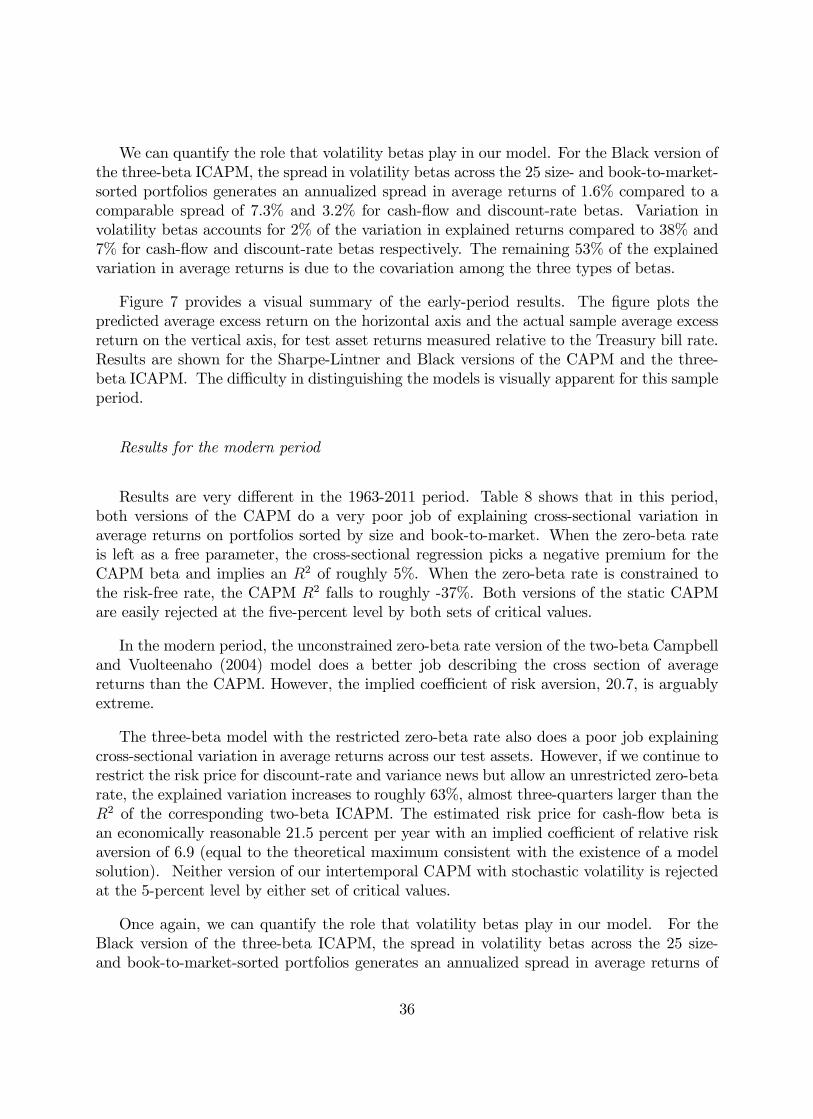
We can quantify the role that volatility betas play in our model. For the Black version ofthe three-beta ICAPM, the spread in volatility betas across the 25 size- and book-to-market-sorted portfolios generates an annualized spread in average returns of 1.6% compared to acomparable spread of 7.3% and 3.2% for cash-�ow and discount-rate betas. Variation involatility betas accounts for 2% of the variation in explained returns compared to 38% and7% for cash-�ow and discount-rate betas respectively. The remaining 53% of the explainedvariation in average returns is due to the covariation among the three types of betas.

Figure 7 provides a visual summary of the early-period results. The �gure plots thepredicted average excess return on the horizontal axis and the actual sample average excessreturn on the vertical axis, for test asset returns measured relative to the Treasury bill rate.Results are shown for the Sharpe-Lintner and Black versions of the CAPM and the three-beta ICAPM. The di¢ culty in distinguishing the models is visually apparent for this sampleperiod.

Results for the modern period

Results are very di¤erent in the 1963-2011 period. Table 8 shows that in this period,both versions of the CAPM do a very poor job of explaining cross-sectional variation inaverage returns on portfolios sorted by size and book-to-market. When the zero-beta rateis left as a free parameter, the cross-sectional regression picks a negative premium for theCAPM beta and implies an R2 of roughly 5%. When the zero-beta rate is constrained tothe risk-free rate, the CAPM R2 falls to roughly -37%. Both versions of the static CAPMare easily rejected at the �ve-percent level by both sets of critical values.

In the modern period, the unconstrained zero-beta rate version of the two-beta Campbelland Vuolteenaho (2004) model does a better job describing the cross section of averagereturns than the CAPM. However, the implied coe¢ cient of risk aversion, 20.7, is arguablyextreme.

The three-beta model with the restricted zero-beta rate also does a poor job explainingcross-sectional variation in average returns across our test assets. However, if we continue torestrict the risk price for discount-rate and variance news but allow an unrestricted zero-betarate, the explained variation increases to roughly 63%, almost three-quarters larger than theR2 of the corresponding two-beta ICAPM. The estimated risk price for cash-�ow beta isan economically reasonable 21.5 percent per year with an implied coe¢ cient of relative riskaversion of 6.9 (equal to the theoretical maximum consistent with the existence of a modelsolution). Neither version of our intertemporal CAPM with stochastic volatility is rejectedat the 5-percent level by either set of critical values.

Once again, we can quantify the role that volatility betas play in our model. For theBlack version of the three-beta ICAPM, the spread in volatility betas across the 25 size-and book-to-market-sorted portfolios generates an annualized spread in average returns of

36

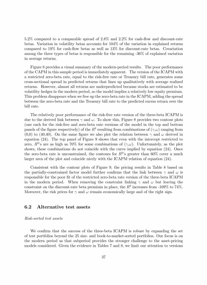
5.2% compared to a comparable spread of 2.8% and 2.2% for cash-�ow and discount-ratebetas. Variation in volatility betas accounts for 104% of the variation in explained returnscompared to 19% for cash-�ow betas as well as 13% for discount-rate betas. Covariationamong the three types of betas is responsible for the remaining -36% of explained variationin average returns.

Figure 8 provides a visual summary of the modern-period results. The poor performanceof the CAPM in this sample period is immediately apparent. The version of the ICAPMwitha restricted zero-beta rate, equal to the risk-free rate or Treasury bill rate, generates somecross-sectional spread in predicted returns that lines up qualitatively with average realizedreturns. However, almost all returns are underpredicted because stocks are estimated to bevolatility hedges in the modern period, so the model implies a relatively low equity premium.This problem disappears when we free up the zero-beta rate in the ICAPM, adding the spreadbetween the zero-beta rate and the Treasury bill rate to the predicted excess return over thebill rate.

The relatively poor performance of the risk-free rate version of the three-beta ICAPM isdue to the derived link between and !. To show this, Figure 8 provides two contour plots(one each for the risk-free and zero-beta rate versions of the model in the top and bottompanels of the �gure respectively) of the R2 resulting from combinations of ( ,!) ranging from(0,0) to (40,40). On the same �gure we also plot the relation between and ! derived inequation (24). The top panel of Figure 9 shows that even with the intercept restricted tozero, R2�s are as high as 70% for some combinations of ( ,!). Unfortunately, as the plotshows, these combinations do not coincide with the curve implied by equation (24). Oncethe zero-beta rate is unconstrained, the contours for R2�s greater than 60% cover a muchlarger area of the plot and coincide nicely with the ICAPM relation of equation (24).

Consistent with the contour plots of Figure 9, the pricing results in Table 8 based onthe partially-constrained factor model further con�rms that the link between and ! isresponsible for the poor �t of the restricted zero-beta rate version of the three-beta ICAPMin the modern period. When removing the constraint linking and ! but leaving theconstraint on the discount-rate beta premium in place, the R2 increases from -109% to 74%.Moreover, the risk prices for and ! remain economically large and of the right sign.

6.2 Alternative test assets

Risk-sorted test assets

We con�rm that the success of the three-beta ICAPM is robust by expanding the setof test portfolios beyond the 25 size- and book-to-market-sorted portfolios. Our focus is onthe modern period as that subperiod provides the stronger challenge to the asset-pricingmodels considered. Given the evidence in Tables 7 and 8, we limit our attention to versions

37

of the CAPM, the 2-beta ICAPM, and the 3-beta ICAPM where the zero-beta rate is leftunconstrained, though we report results for all ten models in the Appendix.

First, we show that our three-beta model not only describes the cross section of characteristic-sorted portfolios but also can explain the average returns on risk-sorted portfolios. The �rstthree columns of Table 9 price the six risk-sorted portfolios described in Table 6 Panel B inconjunction with six of the 25 size- and book-to-market-sorted portfolios of Table 6 Panel A(the low, medium, and high BE/ME portfolios within the small and large ME quintiles) inthe modern period. We �nd that the three-beta ICAPM is not rejected by the data whilethe CAPM is rejected. Importantly, the relatively high R2 for the zero-beta rate version ofthe volatility ICAPM (68%) is not disproportionately due to characteristic-sorted portfolios,as the R2 for the risk-sorted subset (80%) is not only comparable to but actually larger thanthe R2 for the characteristic-sorted subset (68%).24 Though the two-beta ICAPM is notrejected, the R2 is much lower. Appendix Figure 3 provides a graphical summary of theseresults.25

Characteristic and risk-sorted test assets

The next three columns of Table 9 Panel A price the 18 BE/ME-ivol-b��V AR-sortedportfolios described in Table 6 Panel C. These portfolios present an interesting challenge toour model as they incorporate the idiosyncratic risk anomaly of Ang, Hodrick, Xing, andZhang (2006). We �nd that the three-beta ICAPM is not rejected by the data while boththe CAPM and the two-beta ICAPM are strongly rejected. In particular, the three-betaICAPM delivers a relatively high R2 of 49% while the corresponding R2s of the CAPM andthe two-beta ICAPM are less than 15% (with the CAPM picking a negative premium formarket beta). As a consequence, our model can also explain the puzzling idiosyncratic riske¤ect in the cross section of average returns. We provide a visual summary of this successin Appendix Figure 4.

24We report the breakdown of R2 across the risk-sorted and characteristic-sorted subsets in the InternetAppendix.25For completeness, we also examine the ability of our model to explain risk-sorted portfolios in the

early period. Internet Appendix Table 4 prices the six risk-sorted portfolios described in Table 5 Panel Bin conjunction with six of the 25 size- and book-to-market-sorted portfolios of Table 5 Panel A (the low,medium, and high BE/ME portfolios within the small and large ME quintiles) in the early period. Wecontinue to �nd that the three-beta ICAPM modestly improves pricing relative to both the Sharpe-Lintnerand Black versions of the CAPM. Moreover, the relatively high R2 (57%) is not disproportionately due tocharacteristics-sorted portfolios, as the R2 for the risk-sorted subset (68%) is again not only comparableto but actually larger than the R2 for the characteristics-sorted subset (51%). Internet Appendix Figure 2shows this success graphically.

38

Non-equity test assets

Our three-beta model goes some way towards explaining the average returns on non-equity portfolios designed to be highly correlated with aggregate volatility risk, namelythe S&P 100 index straddles of Coval and Shumway (2001). We �rst calculate the expectedreturn on the straddle portfolio based on the estimate of the zero-beta rate volatility ICAPMin Table 8. The contributions to expected quarterly return from the straddle�s cash-�ow,discount-rate, and volatility betas are -2.14%, -1.37%, and -3.15% respectively. As theaverage quarterly realized return on the straddle is -21.66%, an equity-based estimate of thethree-beta model explains roughly 31% of the realized straddle premium.

We then price the straddle in conjunction with both equity and �xed income portfolios.Note that if we were simply to add the straddle position to our analysis, its extreme in-sampleaverage return and volatility would dominate the cross-sectional regression. Therefore, werescale the straddle by forming a portfolio of the straddle and the Treasury Bill. In particular,we hold one seventh of the portfolio in the straddle and the remaining six sevenths in theT-Bill.26 The last three columns of Table 9 Panel A show that our intertemporal CAPM withstochastic volatility is rejected at the 5-percent level when we price the joint cross-sectionof equity, bond, and straddle returns. Both the CAPM and the two-beta ICAPM are alsostrongly rejected. Nevertheless, both the R2 and the pricing measure improve signi�cantly asone moves from the CAPM to the three-beta ICAPM. Appendix Figure 5 provides a visualsummary of the CAPM and ICAPM results, illustrating the di¢ cult challenge posed by theextremely low realized returns on the straddle portfolio.

The �rst three columns of Table 9 Panel B price the cross section of currency portfoliossorted on interest rates. A large literature studies the properties of the currency carrytrade, a strategy that exploits the forward premium puzzle of Fama (1984) by buying highinterest-rate currencies and shorting low interest-rate currencies. The two-beta Campbelland Vuolteenaho (2004) model produces a similar R2 as the CAPM. However, the impliedrisk aversion estimate is quite large at 14.3.

The proportion of variation explained by the three-beta ICAPM is roughly 82%, with arisk aversion estimate of 6.9 (once again equal to the theoretical maximum). Our intertem-poral CAPM with stochastic volatility is not rejected at the 5-percent level by either set ofcritical values. Appendix Figure 6 provides a visual summary of the relative pricing abilityof the CAPM and the volatility ICAPM for currency portfolios.

The second three columns of Table 9 Panel B price the cross section of variance forwards.We �nd that average returns on one-month variance forwards are negative and statisticallysigni�cant. At longer horizons, average returns generally increase, and, for some months,become statistically greater than zero. The three-beta model is not rejected by the data; the26We chose these weights as the volatility of the resulting portfolio is roughly similar to the volatility of the

other assets included in the test. However, our results are qualitatively una¤ected by reasonable variationin these proportions.

39

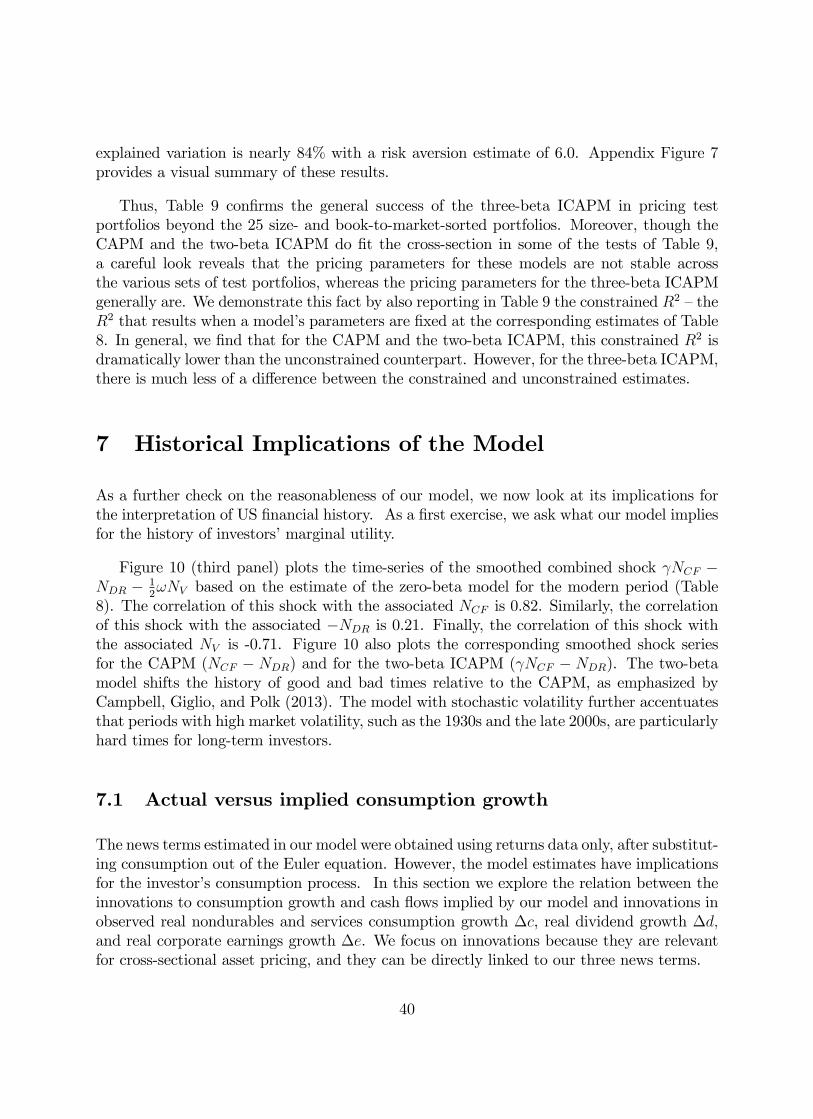
explained variation is nearly 84% with a risk aversion estimate of 6.0. Appendix Figure 7provides a visual summary of these results.

Thus, Table 9 con�rms the general success of the three-beta ICAPM in pricing testportfolios beyond the 25 size- and book-to-market-sorted portfolios. Moreover, though theCAPM and the two-beta ICAPM do �t the cross-section in some of the tests of Table 9,a careful look reveals that the pricing parameters for these models are not stable acrossthe various sets of test portfolios, whereas the pricing parameters for the three-beta ICAPMgenerally are. We demonstrate this fact by also reporting in Table 9 the constrained R2 �theR2 that results when a model�s parameters are �xed at the corresponding estimates of Table8. In general, we �nd that for the CAPM and the two-beta ICAPM, this constrained R2 isdramatically lower than the unconstrained counterpart. However, for the three-beta ICAPM,there is much less of a di¤erence between the constrained and unconstrained estimates.

7 Historical Implications of the Model

As a further check on the reasonableness of our model, we now look at its implications forthe interpretation of US �nancial history. As a �rst exercise, we ask what our model impliesfor the history of investors�marginal utility.

Figure 10 (third panel) plots the time-series of the smoothed combined shock NCF �NDR � 1

2!NV based on the estimate of the zero-beta model for the modern period (Table

8). The correlation of this shock with the associated NCF is 0.82. Similarly, the correlationof this shock with the associated �NDR is 0.21. Finally, the correlation of this shock withthe associated NV is -0.71. Figure 10 also plots the corresponding smoothed shock seriesfor the CAPM (NCF � NDR) and for the two-beta ICAPM ( NCF � NDR). The two-betamodel shifts the history of good and bad times relative to the CAPM, as emphasized byCampbell, Giglio, and Polk (2013). The model with stochastic volatility further accentuatesthat periods with high market volatility, such as the 1930s and the late 2000s, are particularlyhard times for long-term investors.

7.1 Actual versus implied consumption growth

The news terms estimated in our model were obtained using returns data only, after substitut-ing consumption out of the Euler equation. However, the model estimates have implicationsfor the investor�s consumption process. In this section we explore the relation between theinnovations to consumption growth and cash �ows implied by our model and innovations inobserved real nondurables and services consumption growth �c, real dividend growth �d;and real corporate earnings growth �e. We focus on innovations because they are relevantfor cross-sectional asset pricing, and they can be directly linked to our three news terms.

40

As we report in the Appendix, our model implies that consumption innovations are givenby

�ct+1 � Et�ct+1 = (rt+1 � Etrt+1)� ( � 1)NDR;t+1 � ( � 1)1

2

!

1� NV;t+1; (30)

while cash �ow news is determined by equation (17). We can easily compute both seriesby appropriately combining the estimated VAR innovations with our estimates for and !,respectively 6.9 and 20.9. Note, however, that the EIS parameter , which a¤ects the impliedconsumption growth innovations, is not pinned down by our VAR estimation. Therefore, wecalibrate it to three di¤erent values, 0.5, 1.0, and 1.5.

We start by comparing the implied consumption innovations (�ct+1 � Et�ct+1) to ob-served innovations in real log consumption growth, real log dividend growth and real logearnings growth. We construct consumption growth using nondurable and services datafrom the BEA, and obtain long-term dividend and earnings data from Professor RobertShiller�s website. We construct consumption, dividends and earnings innovations by takingthe residuals of an AR(1) regression for each series. To maximize the length of our timeseries and to avoid the issue of seasonality in dividends and earnings, we work here withyearly data, from 1930 to 2011. All the results are robust to using smoothed quarterly datafor the available periods.

Panel A of Table 10 reports the standard deviations of six series: innovations in ac-tual consumption, dividends and earnings growth, and implied innovations in consumptionunder the three calibration for (0.5, 1, 1.5). The table shows that the implied consump-tion innovation series are more volatile than actual consumption innovations. The fact thataggregate consumption growth is smooth is well known; as pointed out for example in Mal-loy, Moskowitz and Vissing-Jørgensen (2009), aggregate consumption growth may not bethe right benchmark for our asset pricing model because it includes consumption of non-stockholder consumers.27 However, the table also shows that implied consumption growthis about as volatile as earnings and dividend growth innovations (depending on ).

Panel B of Table 10 reports the correlations between the consumption innovation seriesimplied by our model and the observed consumption, dividend and earnings growth innova-tions. The left panel reports the correlations of the raw series, while the right panel reportscorrelations of exponentially-weighted moving averages of each series, which are useful toshow the low-frequency comovements. The table shows that our implied consumption seriesare positively correlated with the realizations of consumption, dividend and earnings growth.The strength of the correlations increases in almost all cases when looking at the smoothedseries.

To gauge the low-frequency comovements between these series better, Appendix Figure10 shows the exponentially-weighted moving average of the series of implied consumption in-

27In theory, we could test the model directly using data on stockholder consumption, but the time seriesavailable spans 20 years, which is not long enough to be used to estimate the news terms and test our model.

41

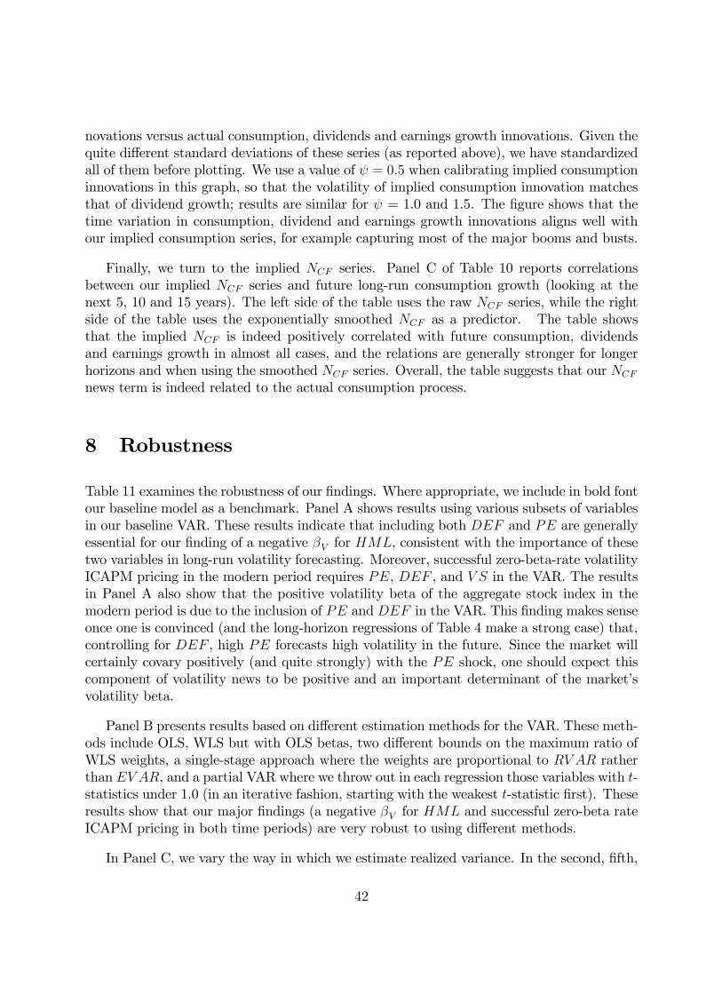
novations versus actual consumption, dividends and earnings growth innovations. Given thequite di¤erent standard deviations of these series (as reported above), we have standardizedall of them before plotting. We use a value of = 0:5 when calibrating implied consumptioninnovations in this graph, so that the volatility of implied consumption innovation matchesthat of dividend growth; results are similar for = 1.0 and 1.5. The �gure shows that thetime variation in consumption, dividend and earnings growth innovations aligns well withour implied consumption series, for example capturing most of the major booms and busts.

Finally, we turn to the implied NCF series. Panel C of Table 10 reports correlationsbetween our implied NCF series and future long-run consumption growth (looking at thenext 5, 10 and 15 years). The left side of the table uses the raw NCF series, while the rightside of the table uses the exponentially smoothed NCF as a predictor. The table showsthat the implied NCF is indeed positively correlated with future consumption, dividendsand earnings growth in almost all cases, and the relations are generally stronger for longerhorizons and when using the smoothed NCF series. Overall, the table suggests that our NCF

news term is indeed related to the actual consumption process.

8 Robustness

Table 11 examines the robustness of our �ndings. Where appropriate, we include in bold fontour baseline model as a benchmark. Panel A shows results using various subsets of variablesin our baseline VAR. These results indicate that including both DEF and PE are generallyessential for our �nding of a negative �V for HML, consistent with the importance of thesetwo variables in long-run volatility forecasting. Moreover, successful zero-beta-rate volatilityICAPM pricing in the modern period requires PE, DEF , and V S in the VAR. The resultsin Panel A also show that the positive volatility beta of the aggregate stock index in themodern period is due to the inclusion of PE and DEF in the VAR. This �nding makes senseonce one is convinced (and the long-horizon regressions of Table 4 make a strong case) that,controlling for DEF , high PE forecasts high volatility in the future. Since the market willcertainly covary positively (and quite strongly) with the PE shock, one should expect thiscomponent of volatility news to be positive and an important determinant of the market�svolatility beta.

Panel B presents results based on di¤erent estimation methods for the VAR. These meth-ods include OLS, WLS but with OLS betas, two di¤erent bounds on the maximum ratio ofWLS weights, a single-stage approach where the weights are proportional to RV AR ratherthan EV AR, and a partial VAR where we throw out in each regression those variables with t-statistics under 1.0 (in an iterative fashion, starting with the weakest t-statistic �rst). Theseresults show that our major �ndings (a negative �V for HML and successful zero-beta rateICAPM pricing in both time periods) are very robust to using di¤erent methods.

In Panel C, we vary the way in which we estimate realized variance. In the second, �fth,

42

and sixth columns of the Table, we estimate the VAR using annual data. Thus our estimateof realized variance re�ects information over the entire year. In columns three and �ve, wecompute the realized variance of monthly returns rather than the realized variance of dailyreturns as in our benchmark speci�cation. In the fourth and six columns, we simply sumsquared monthly returns. Across Panel C, the R2s of the zero-beta rate ICAPM remain highin the modern period.

In Panel D, we alter the set of variables included in the VAR as a response to the concernof Chen and Zhao (2009) that VAR-based forecasts are sensitive to this choice. (See alsoEngsted, Pedersen, and Tanggaard 2012 for a clarifying discussion of this issue.) We �rstexplore di¤erent ways to measure the market�s valuation ratio. In the second column of theTable, we replace PE with PERe al where we construct the price-earnings ratio by de�atingboth the price and the earnings series by the CPI before taking their ratio. In the thirdcolumn, we use the log price-dividend ratio, PD, instead of PE. In column four, we replacePE with PERe al and the CPI in�ation rate, INFL. Panel D also explores adding twoadditional state variables. In column �ve, we add CAY (Lettau and Ludvigson (2001)) tothe VAR as CAY is known to be a strong predictor of future market returns. Column sixadds the quarterly FIGARCH forecast to the VAR as Table 4 Panel B documents thatGARCH-based methods are useful predictors of future market return variance.

Column seven adds the volatility of the term spread (TY V ol) to the list of state variablesbased on the evidence in Fornari and Mele (2011) that this variable contains informationabout time-varying expected returns. In particular, following Fornari and Mele (2011), weadd the mean absolute monthly change in the term spread over the previous twelve months.28

In results reported in the online appendix, we show that TY V ol is not incrementally im-portant for forecasting either the �rst or second moment of the real market return. In fact,even if we exclude some or all of PE, TY , DEF , or V S from the VAR, TY V ol never comesin signi�cantly. However, TY V ol does help forecast DEF . Nevertheless, adding TY V OLto the VAR does not qualitatively change the conclusions of the pricing tests. In total, thisPanel con�rms that our �nding of a negative �V for HML and successful zero-beta rateICAPM pricing in both time periods is generally robust to these variations.

In Panel E, we study the out-of-sample properties of our model. In particular, we estimateour baseline VAR on an expanding window, using the estimates in each window to generatenews terms for the quarter ahead. Since the interesting pricing results are in the modernperiod, our initial window is the 1926:2 to 1963:2 period, so that the �rst out-of-sample newsrealizations occur in 1963:3, corresponding to the �rst data point in the modern period.We �nd that the out-of-sample news terms are extremely correlated with their in-samplecounterparts. Speci�cally, the correlations are 0.81, 0.97, and 0.82 for the cash-�ow, discount-rate, and volatility news terms respectively. Table 11 Panel E documents that the pricing ofthe out-of-sample news terms is very consistent with the full-sample results.29

28Results are robust to measuring the volatility of the monthly term spread over the last year instead.29Internet Appendix Figure 8 provides a visual summary of these out-of-sample pricing results for the

CAPM and three-beta ICAPM.

43

In Panel F, we explore using alternative proxies for the wealth portfolio. In particular,we replace the market returns with the return on a delevered market portfolio that combinesTreasury Bills and the market in various constant proportions. By doing so, we are able toassess how varying the volatility of this central series a¤ects our results. The three speci�cdelevered portfolios we examine have 80%, 60%, or 40% invested in the market. We �ndthat the cross-sectional �t of our model remains high, with R2s in the early period essentiallyuna¤ected and R2s in the modern period increasing in all but the extreme delevered portfolio.Perhaps not surprisingly, the estimated risk aversion parameter increases as the degree ofdelevering increases. In the modern period, delevering the market portfolio by 20% resultsin a risk aversion estimate of 9.99, delevering by 40% requires risk aversion of 14.51, anddelevering by 80% generates a risk aversion estimate of 18.44.

Panel G reports the results when we vary � and the excess zero-beta rate. One mightargue that our excess zero-beta rate estimate of 112 basis points a quarter is too high tobe consistent with equilibrium. Fortunately, we �nd that R2s remain reasonable for excesszero-beta rates that are as low as 50 bps/quarter when � takes only a slightly lower value,0.94.

Panels H and I present information to help us better understand the volatility betas wehave estimated for the market as a whole, and for value stocks relative to growth stocks.Panel H reports components of RMRF andHML�s �V in each period (estimated either withWLS or OLS). Speci�cally, these results use the elements of the vector de�ned in equation(17) and the corresponding VAR shock to measure how each shock contributes to the �V inquestion. Panel H documents, consistent with Panel A, that the excess return on the markethas a positive volatility beta in the modern period due in part to the PE state variable. Theresults in Panel H also show that all of the non-zero components of HML�s �V in the modernperiod are negative. This �nding is comforting as it further con�rms that our negative HMLbeta �nding is robust. Panel H also reports OLS estimates of simple betas on RV AR and the15-year horizon FIGARCH forecast (FIG60) for HML and the excess market return. TheHML betas based on these two simple proxies have the same sign as our more sophisticatedand more appropriate measure of volatility news. However, conclusions about the relevanceof volatility risk for the value e¤ect clearly depend on measuring the long-run component ofvolatility well.

Finally, Panel I reports time-series regressions of HML on NV;t by itself as well as onall three factors together. We �nd that NV;t explains over 20% of HML�s returns in themodern period. The three news factors together explain slightly over 28%. Thus our modelis able to explain not only the cross-sectional variation in average returns of the 25 size- andbook-to-market-sorted portfolios of Fama and French (1993) but also a signi�cant amountof time series variation in realized returns on the key factor that they argue is multifactor-minimum-variance (Fama and French, 1996).

44

9 Conclusion

We extend the approximate closed-form intertemporal capital asset pricing model of Camp-bell (1993) to allow for stochastic volatility. Our model recognizes that an investor�s invest-ment opportunities may deteriorate either because expected stock returns decline or becausethe volatility of stock returns increases. A conservative long-term investor will wish to hedgeagainst both types of changes in investment opportunities; thus, a stock�s risk is determinednot only by its beta with unexpected market returns and news about future returns (orequivalently, news about market cash �ows and discount rates), but also by its beta withnews about future market volatility. Although our model has three dimensions of risk, theprices of all these risks are determined by a single free parameter, the coe¢ cient of relativerisk aversion.

Our implementation models the return on the aggregate stock market as one elementof a vector autoregressive (VAR) system; the volatility of all shocks to the VAR is anotherelement of the system. The empirical implementation of our VAR reveals new low-frequencymovements in market volatility tied to the default spread. We show that the negativepost-1963 CAPM alphas of growth stocks are justi�ed because these stocks hedge long-term investors against both declining expected stock returns, and increasing volatility. Theaddition of volatility risk to the model helps it �t the cross-section of value and growthstocks, and small and large stocks, with a moderate, economically reasonable value of riskaversion.

We confront our model with portfolios of stocks sorted by past betas with the marketreturn and volatility, and portfolios sorted both by characteristics (book-market ratios andidiosyncratic volatility) and past volatility betas. We also use the model to �t the averagereturns on non-equity test assets, including corporate bonds, equity index option straddles,interest-rate sorted currency portfolios, and variance forwards. The explanatory power ofthe model is quite good across all these sets of test assets, with stable parameter estimates,although the extremely low average return on equity index options remains an empiricalchallenge.

Our empirical work is limited in two important respects. First, we have assumed thatthe wealth portfolio of a representative investor can be adequately proxied by a diversi�edequity portfolio. We have checked that our �ndings are robust to the use of a deleveredequity portfolio, but to the extent that other risky assets, such as corporate bonds or evenhuman capital, are important constituents of wealth, this assumption may be inadequate.It will be of interest to explore stochastic volatility in alternative proxies for the wealthportfolio.

Second, we test only the unconditional implications of the model and do not evaluate itsconditional implications. A full conditional test is likely to be a challenging hurdle for themodel. To see why, recall that we assume a rational long-term investor always holds 100%

45

of his or her assets in equities. However, time-variation in real stock returns generally givesthe long-term investor an incentive to shift the relative weights on cash and equity, unlessreal interest rates and market volatility move in exactly the right way to make the equitypremium proportional to market volatility. Although we do not explicitly test whether thisis the case, early papers by Campbell (1987) and Harvey (1989, 1991) and a recent reviewby Lettau and Ludvigson (2010) reject this proportionality restriction.

One way to support the assumption of constant 100% equity investment is to invokebinding leverage constraints. Indeed, in the modern sample, the Black (1972) version of ourthree-beta model is consistent with this interpretation as the estimated di¤erence betweenthe zero-beta and risk-free rates is positive, statistically signi�cant, and economically large.However, while our estimates imply that the leverage constraint is unconditionally bindingfor a long-horizon investor given the risk characteristics of the market portfolio in the modernsample, they do not imply that it is always conditionally binding in every period.

Both these limitations are opportunities for future research. And our model does directlyanswer the interesting microeconomic question: Are there reasonable preference parametersthat would make a long-term investor, constrained to invest 100% in equity, content to holdthe market rather than tilting towards value stocks or other high-return stock portfolios?Our answer is clearly yes.

46

References

Adrian, Tobias and Joshua Rosenberg, 2008, �Stock Returns and Volatility: Pricing theShort-Run and Long-Run Components of Market Risk�, Journal of Finance 63:2997�3030.

Andersen, Torben G., Tim Bollerslev, Francis X. Diebold, and Paul Labys, 2003, �Modelingand Forecasting Realized Volatility�, Econometrica 71:579�625.

Andersen, Torben, Tim Bollerslev, Peter F. Christo¤ersen and Francis X. Diebold, 2006,�Volatility and Correlation Forecasting�, in Graham Elliott, Clive W.J. Granger andAllan Timmermann (eds), Handbook of Economic Forecasting, Vol I.

Ang, Andrew, Robert J. Hodrick, Yuhang Xing, and Xiaoyan Zhang, 2006, �The Cross-Section of Volatility and Expected Returns�, Journal of Finance 61:259�299.

Baillie, Richard T., Tim Bollerslev and Hans Ole Mikkelsen, 1996, �Fractionally integratedgeneralized autoregressive conditional heteroskedasticity�, Journal of Econometrics74:3�30.

Bali, Turan and Nusret Cakici, 2009, �Idiosyncratic Volatility and the Cross Section ofExpected Stock Returns�, Journal of Financial and Quantitative Analysis 43:29�58.

Bansal, Ravi and Amir Yaron, 2004, �Risks for the Long Run�, Journal of Finance 59:1481�1509.

Bansal, Ravi, Dana Kiku and Amir Yaron, 2012, �An Empirical Evaluation of the Long-RunRisks Model for Asset Prices�, Critical Finance Review 1:183�221.

Bansal, Ravi, Dana Kiku, Ivan Shaliastovich and Amir Yaron, 2013, �Volatility, the Macro-economy and Asset Prices�, Journal of Finance forthcoming.

Barinov, Alexander, 2013, �Idiosyncratic Volatility, Growth Options, and the Cross-Sectionof Returns�, working paper, University of Georgia.

Barndor¤-Nielsen, Ole E. and Neil Shephard, 2002, �Econometric Analysis of RealizedVolatility and Its Use in Estimating Stochastic Volatility Models�, Journal of the RoyalStatistical Society B, 64(2):253�280.

Beeler, Jason and John Y. Campbell, 2012, �The Long-Run Risks Model and AggregateAsset Prices: An Empirical Assessment�, Critical Finance Review 1:141�182.

Black, Fisher, 1972, �Capital Market Equilibrium with Restricted Borrowing�, Journal ofBusiness 45:444�454.

Black, Fisher, 1976, �Studies of Stock Price Volatility Changes�, Proceedings of the 1976Meetings of the American Statistical Association, Business and Economic StatisticsSection, Washington 177�181.

47

Bollerslev, Tim, 1986, �Generalized Autoregressive Conditional Heteroskedasticity�, Jour-nal of Econometrics 31:307�327.

Bollerslev, Tim and Hans Ole Mikkelsen, 1996, �Modeling and Pricing Long Memory inStock Market Volatility�, Journal of Econometrics 73:151�184.

Breeden, Douglas T., 1979, �An Intertemporal Asset Pricing Model with Stochastic Con-sumption and Investment Opportunities�, Journal of Financial Economics 7:265�296.

Calvet, Laurent and Adlai Fisher, 2007, �Multifrequency News and Stock Returns�, Journalof Financial Economics 86:178�212.

Campbell, John Y., 1987, �Stock Returns and the Term Structure�, Journal of FinancialEconomics 18:373�399.

Campbell, John Y., 1993, �Intertemporal Asset Pricing Without Consumption Data�,American Economic Review 83:487�512.

Campbell, John Y., 1996, �Understanding Risk and Return�, Journal of Political Economy104:298�345.

Campbell, John Y., Stefano Giglio, and Christopher Polk, 2013, �Hard Times�, Review ofAsset Pricing Studies 3:95�132.

Campbell, John Y., Stefano Giglio, Christopher Polk, and Robert Turley, 2014, �Ap-pendix to An Intertemporal CAPM with Stochastic Volatility�, available online athttp://scholar.harvard.edu/campbell/publications.

Campbell, John Y. and Ludger Hentschel, 1992, �No News is Good News: An Asymmet-ric Model of Changing Volatility in Stock Returns�, Journal of Financial Economics31:281�318.

Campbell, John Y., Christopher Polk, and Tuomo Vuolteenaho, 2010, �Growth or Glamour?Fundamentals and Systematic Risk in Stock Returns� Review of Financial Studies23:305�344.

Campbell, John Y. and Robert J. Shiller, 1988a, �The Dividend-Price Ratio and Expecta-tions of Future Dividends and Discount Factors�, Review of Financial Studies 1:195�228.

Campbell, John Y. and Robert J. Shiller, 1988b, �Stock Prices, Earnings, and ExpectedDividends�, Journal of Finance 43:661�676.

Campbell, John Y. and Glen B. Taksler, 2003, �Equity Volatility and Corporate BondYields�, Journal of Finance 58:2321�2349.

Campbell, John Y. and Tuomo Vuolteenaho, 2004, �Bad Beta, Good Beta�, AmericanEconomic Review 94:1249�1275.

48

Chacko, George and Luis M. Viceira, 2005, �Dynamic Consumption and Portfolio Choicewith Stochastic Volatility in Incomplete Markets�, Review of Financial Studies 18:1369�1402.

Chen, Joseph, 2003, �Intertemporal CAPM and the Cross Section of Stock Returns�, un-published paper, University of California Davis.

Chen, Zhanhui and Ralitsa Petkova, 2014, Does Idiosyncratic Volatility Proxy for RiskExposure?, Review of Financial Studies 25:2745�2787.

Chen, Long and Xinlei Zhao, 2009, �Return Decomposition�, Review of Financial Studies22:5213�5249.

Christiansen, Charlotte, Maik Schmeling and Andreas Schrimpf, 2012, �A ComprehensiveLook at Financial Volatility Prediction by Economic Variables�, Journal of AppliedEconometrics 27: 956-977.

Christie, Andrew, �The Stochastic Behavior of Common Stock Variances �Value, Leverage,and Interest Rates E¤ects�, Journal of Financial Economics 10:407�432.

Cochrane, John H., 2008, �The Dog That Did Not Bark: A Defense of Return Predictabil-ity�, Review of Financial Studies 21:1533-1575.

Cochrane, John H., 2011, �Presidential Address: Discount Rates�, Journal of Finance66:1047�1108.

Coval, Josh, and Tyler Shumway, 2001, �Expected Option Returns�, Journal of Finance56:983�1009.

Daniel, Kent and Sheridan Titman, 1997, �Evidence on the Characteristics of Cross-sectional Variation in Common Stock Returns�, Journal of Finance 52:1�33.

Daniel, Kent and Sheridan Titman, 2012, �Testing Factor-Model Explanations of MarketAnomalies�, Critical Finance Review 1:103�139.

Darolles, Serge, Christian Gourieroux, and Joann Jasiak, 2006, �Structural Laplace Trans-form and Compound Autoregressive Models�, Journal of Time Series Analysis 27,477�504.

Davis, James L., Eugene F. Fama, and Kenneth R. French, �Characteristics, Covariances,and Average Returns: 1929 to 1997�, Journal of Finance 55:389�406.

Du¤ee, Greg, 2005, �Time-Variation in the Covariance Between Stock Returns and Con-sumption Growth�, Journal of Finance 60:1673�172.

Du¢ e, Darrell and Kenneth J. Singleton, 1997, �An Econometric Model of the Term Struc-ture of Interest Rate Swap Yields�, Journal of Finance 52: 1287-1321.

49

Engle, Robert F, 1982, �Autoregressive Conditional Heteroscedasticity with Estimates ofthe Variance of United Kingdom In�ation,�Econometrica 50: 987�1007.

Engle, Robert F., Eric Ghysels and Bumjean Sohn, 2013, �Stock Market Volatility andMacroeconomic Fundamentals�, Review of Economics and Statistics 95: 776�797.

Engsted, Tom, Thomas Q. Pedersen, and Carsten Tanggaard, 2012, �Pitfalls in VAR BasedReturn Decompositions: A Clari�cation�, Journal of Banking and Finance 36: 1255-1265..

Epstein, Lawrence and Stanley Zin, 1989, �Substitution, Risk Aversion, and the TemporalBehavior of Consumption and Asset Returns: A Theoretical Framework�, Economet-rica 57:937�69.

Epstein, Lawrence, Emmanuel Farhi, and Tomasz Strzalecki, 2013, �How Much Would YouPay to Resolve Long-Run Risk?�, unpublished paper, Boston University and HarvardUniversity.

Eraker, Bjorn, 2008, �A¢ ne General Equilibrium Models�, Management Science 54:2068�2080.

Eraker, Bjorn and Ivan Shaliastovich, 2008, �An Equilibrium Guide to Designing A¢ nePricing Models�, Mathematical Finance 18:519�543.

Eraker, Bjorn and Wenyu Wang, 2011, �Dynamic Present Values and the IntertemporalCAPM�, University of Wisconsin working paper.

Fama, Eugene F., 1984, �Forward and Spot Exchange Rates�, Journal of Monetary Eco-nomics 14:319�38.

Fama, Eugene F. and Kenneth R. French, 1992, �The Cross-Section of Expected StockReturns�, Journal of Finance 47: 427-465.

Fama, Eugene F. and Kenneth R. French, 1993, �Common Risk Factors in the Returns onStocks and Bonds�, Journal of Financial Economics 33:3�56.

Fama, Eugene F. and Kenneth R. French, 1996, �Multifactor Explanations of Asset PricingAnomalies�, Journal of Finance 51:55�84.

Fornari, Fabio and Antonio Mele, 2011, �Financial Volatility and Economic Activity�,unpublished paper, University of Lugano.

French, Kenneth, G. William Schwert, and Robert F. Stambaugh, 1987, �Expected StockReturns and Volatility�, Journal of Financial Economics 19:3�29.

Fu, Fangjian, 2009, �Idiosyncratic Risk and the Cross-Section of Expected Stock Returns�,Journal of Financial Economics 91:24�37.

50

Garcia, Rene, Eric Renault, and A. Semenov, 2006, �Disentangling Risk Aversion andIntertemporal Substitution�, Finance Research Letters 3:181�193.

Ghysels, Eric, Andrew C. Harvey and Eric Renault, 1996, �Stochastic Volatility�, in G.S.Maddala and C.R. Rao eds. Handbook of Statistics Vol. 14, 119�191, North-Holland.

Hansen, Lars Peter, 2012, �Dynamic Valuation DecompositionWithin Stochastic Economies�,Econometrica 80:911�967.

Hansen, Lars Peter, 2014, �Uncertainty Inside and Outside Economic Models�, unpublishedNobel Lecture, University of Chicago.

Hansen, Lars Peter, John C. Heaton, J. Lee, and Nicholas Roussanov, 2007, �IntertemporalSubstitution and Risk Aversion�, in J.J. Heckman and E.E. Leamer eds. Handbook ofEconometrics Vol. 6A, 3967�4056, North-Holland.

Hansen, Lars Peter, John C. Heaton, and Nan Li, 2008, �Consumption Strikes Back?Measuring Long-Run Risk�, Journal of Political Economy 116:260�302.

Harvey, Campbell, 1989, �Time-Varying Conditional Covariances in Tests of Asset PricingModels�, Journal of Financial Economics 24:289�317.

Harvey, Campbell, 1991, �TheWorld Price of Covariance Risk�, Journal of Finance 46:111�157.

Heston, Steven L., 1993, �A Closed-Form Solution for Options with Stochastic Volatilitywith Applications to Bond and Currency Options�, Review of Financial Studies 6:327�343.

Hull, John, Mirela Predescu and Alan White, 2004, �The Relationship Between CreditDefault Swap Spreads, Bond Yields, and Credit Rating Announcements,�Journal ofBanking and Finance 28:2789-2811.

Kandel, Shmuel and Robert Stambaugh, 1991, �Asset Returns and Intertemporal Prefer-ences�, Journal of Monetary Economics 27:39�71.

Krishnamurthy, Arvind and Annette Vissing-Jorgensen, 2012, �The Aggregate Demand forTreasury Debt�, Journal of Political Economy 120:233�267.

Lettau, Martin and Sydney C. Ludvigson, 2010, �Measuring and Modeling Variation in theRisk-Return Trade-o¤�, Chapter 11 in Yacine Ait-Sahalia and Lars Peter Hansen eds.Handbook of Financial Econometrics, Elsevier, 617�690.

Lewellen, Jonathan, Stefan Nagel, and Jay Shanken, 2010, �A Skeptical Appraisal of AssetPricing Tests�, Journal of Financial Economics 96:175�194.

Liu, Jun, 2007, �Portfolio Selection in Stochastic Environments�, Review of Financial Stud-ies 20:1�39.

51

Lustig, Hanno, Nikolai Roussanov, and Adrien Verdelhan, 2011, �Common Risk Factors inCurrency Markets�, Review of Financial Studies 24:3731�3777.

Malloy, Christopher J., Tobias J. Moskowitz, and Annette Vissing-Jørgensen, 2009, �Long-Run Stockholder Consumption Risk and Asset Returns�, Journal of Finance, 64: 2427�2479.

McQuade, Timothy J., 2012, �Stochastic Volatility and Asset Pricing Puzzles�, HarvardUniversity working paper.

Meddahi, Nour and Eric Renault, 2004, �Temporal Aggregation of Volatility Models�,Journal of Econometrics 119:355�379.

Merton, Robert C., 1973, �An Intertemporal Capital Asset Pricing Model�, Econometrica41:867�887.

Paye, Bradley, 2012, �Deja Vol: Predictive Regressions for Aggregate Stock Market Volatil-ity using Macroeconomic Variables�, Journal of Financial Economics 106: 527�546.

Poon, Ser-Huang, and Clive W. J. Granger, 2003, �Forecasting Volatility in FinancialMarkets: A Review�, Journal of Economic Literature 41:478�539.

Restoy, Ferdo, and Philippe Weil, 1998, �Approximate Equilibrium Asset Prices�, NBERWorking Paper 6611.

Restoy, Ferdo, and Philippe Weil, 2011, �Approximate Equilibrium Asset Prices�, Reviewof Finance 15:1�28.

Schwert, William, 1989, �Why Does Stock Market Volatility Change Over Time?�, Journalof Finance 44:1115�1153.

Sohn, Bumjean, 2010, �Stock Market Volatility and Trading Strategy Based Factors�, un-published paper, Georgetown University.

Tallarini, T., 2000, �Risk Sensitive Real Business Cycles�, Journal of Monetary Economics45:507�532.

Tauchen, George and Robert Hussey, 1991, �Quadrature-Based Methods for ObtainingApproximate Solutions to Nonlinear Asset Pricing Models�, Econometrica 59:317�396.

52

Table 1: VAR EstimationThe table shows the WLS parameter estimates for a first-order VAR model. The statevariables in the VAR include the log real return on the CRSP value-weight index (rM), therealized variance (RV AR) of within-quarter daily simple returns on the CRSP value-weightindex, the log ratio of the S&P 500’s price to the S&P 500’s ten-year moving average ofearnings (PE), the term yield spread (TY ) in percentage points, measured as the differencebetween the log yield on the ten-year US constant-maturity bond and the log yield onthe three-month US Treasury Bill, the default yield spread (DEF ) in percentage points,measured as the difference between the log yield on Moody’s BAA bonds and the log yieldon Moody’s AAA bonds, and the small-stock value spread (V S), the difference in the logbook-to-market ratios of small value and small growth stocks. The small-value and small-growth portfolios are two of the six elementary portfolios constructed by Davis et al. (2000).For the sake of interpretation, we estimate the VAR in two stages. Panel A reports theWLS parameter estimates of a first-stage regression forecasting RV AR with the VAR statevariables. The forecasted values from this regression are used in the second stage of theestimation procedure as the state variable EV AR, replacing RV AR in the second-stageVAR. Panel B reports WLS parameter estimates of the full second-stage VAR. Initial WLSweights on each observation are inversely proportional to RV ARt and EV ARt in the first andsecond stages respectively and are then shrunk to equal weights so that the maximum ratio ofactual weights used is less than or equal to five. Additionally, the forecasted values for bothRV AR and EV AR are constrained to be positive. In Panels A and B, the first seven columnsreport coeffi cients on an intercept and the six explanatory variables, and the remainingcolumn shows the implied R2 statistic for the unscaled model. Bootstrapped standard errorsthat take into account the uncertainty in generating EV AR are in parentheses. Panel C ofthe table reports the correlation ("Corr/std") and autocorrelation ("Autocorr.") matricesof both the unscaled and scaled shocks from the second-stage VAR; the correlation matrixreports shock standard deviations on the diagonal. The sample period for the dependentvariables is 1926.3-2011.4, 342 quarterly data points.

Panel A: Forecasting Quarterly Realized Variance (RV ARt+1)Constant rM,t RV ARt PEt TYt DEFt V St R2%-0.020 -0.004 0.394 0.006 0.000 0.006 0.001 36.88%(0.008) (0.005) (0.064) (0.002) (0.001) (0.001) (0.002)

53

Panel B: VAR EstimatesSecond stage Constant rM,t EV ARt PEt TYt DEFt V St R2%

rM,t+1 0.219 0.057 1.249 -0.054 0.004 -0.010 -0.032 2.85%(0.119) (0.068) (2.276) (0.034) (0.008) (0.023) (0.035)

EV ARt+1 -0.016 -0.002 0.440 0.005 0.000 0.004 0.002 58.93%(0.007) (0.001) (0.064) (0.002) (0.000) (0.001) (0.002)

PEt+1 0.154 0.138 1.136 0.955 0.004 -0.012 -0.015 94.34%(0.114) (0.066) (2.178) (0.032) (0.007) (0.022) (0.033)

TYt+1 -0.047 -0.097 5.091 0.030 0.820 0.166 0.004 76.56%(0.548) (0.337) (11.342) (0.158) (0.036) (0.112) (0.156)

DEFt+1 0.191 -0.383 6.597 -0.056 0.000 0.834 0.067 88.96%(0.264) (0.151) (4.856) (0.073) (0.017) (0.050) (0.075)

V St+1 0.138 0.075 3.048 -0.017 -0.004 -0.004 0.939 93.94%(0.107) (0.064) (2.085) (0.030) (0.007) (0.021) (0.031)

54

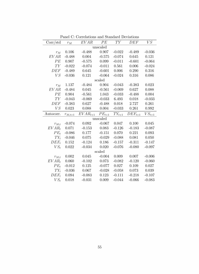
Panel C: Correlations and Standard DeviationsCorr/std rM EV AR PE TY DEF V S

unscaledrM 0.106 -0.488 0.907 -0.022 -0.489 -0.036

EV AR -0.488 0.004 -0.575 -0.074 0.645 0.121PE 0.907 -0.575 0.099 -0.011 -0.601 -0.064TY -0.022 -0.074 -0.011 0.561 0.006 -0.024

DEF -0.489 0.645 -0.601 0.006 0.290 0.316V S -0.036 0.121 -0.064 -0.024 0.316 0.086

scaledrM 1.137 -0.484 0.904 -0.043 -0.383 0.023

EV AR -0.484 0.045 -0.561 -0.069 0.627 0.088PE 0.904 -0.561 1.043 -0.033 -0.488 0.004TY -0.043 -0.069 -0.033 6.493 0.018 -0.033

DEF -0.383 0.627 -0.488 0.018 2.727 0.261V S 0.023 0.088 0.004 -0.033 0.261 0.992

Autocorr. rM,t+1 EV ARt+1 PEt+1 TYt+1 DEFt+1 V St+1

unscaledrM,t -0.074 0.092 -0.067 0.047 0.100 0.045

EV ARt 0.071 -0.153 0.083 -0.126 -0.183 -0.087PEt -0.086 0.177 -0.151 0.070 0.221 0.093TYt -0.046 0.075 -0.029 -0.088 0.081 0.050

DEFt 0.152 -0.124 0.186 -0.157 -0.311 -0.147V St 0.022 -0.034 0.020 -0.076 -0.080 -0.097

scaledrM,t 0.002 0.045 -0.004 0.009 0.007 -0.006

EV ARt 0.060 -0.102 0.073 -0.082 -0.120 -0.060PEt -0.012 0.125 -0.077 0.027 0.109 0.027TYt -0.036 0.067 -0.028 -0.058 0.073 0.039

DEFt 0.094 -0.083 0.123 -0.111 -0.218 -0.107V St 0.018 -0.031 0.009 -0.044 -0.066 -0.083

55

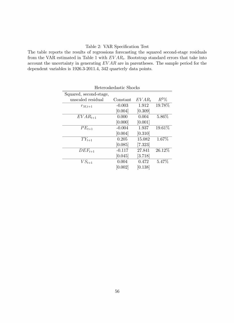
Table 2: VAR Specification TestThe table reports the results of regressions forecasting the squared second-stage residualsfrom the VAR estimated in Table 1 with EV ARt. Bootstrap standard errors that take intoaccount the uncertainty in generating EV AR are in parentheses. The sample period for thedependent variables is 1926.3-2011.4, 342 quarterly data points.

Heteroskedastic ShocksSquared, second-stage,unscaled residual Constant EV ARt R2%

rM,t+1 -0.003 1.912 19.78%[0.004] [0.309]

EV ARt+1 0.000 0.004 5.86%[0.000] [0.001]

PEt+1 -0.004 1.937 19.61%[0.004] [0.310]

TYt+1 0.205 15.082 1.67%[0.085] [7.323]

DEFt+1 -0.117 27.841 26.12%[0.045] [3.718]

V St+1 0.004 0.472 5.47%[0.002] [0.138]

56

Table 3: Cash-flow, Discount-rate, and Variance News for the Market PortfolioThe table shows the properties of cash-flow news (NCF ), discount-rate news (NDR), andvolatility news (NV ) implied by the VARmodel of Table 1. The upper-left section of the tableshows the covariance matrix of the news terms. The upper-right section shows the correlationmatrix of the news terms with standard deviations on the diagonal. The lower-left sectionshows the correlation of shocks to individual state variables with the news terms. The lower-right section shows the functions (e1′+ e1′λDR, e1′λDR, e2′λV ) that map the state-variableshocks to cash-flow, discount-rate, and variance news. We define λDR ≡ ρΓ(I − ρΓ)−1 andλV ≡ ρ(I−ρΓ)−1, where Γ is the estimated VAR transition matrix from Table 1 and ρ is setto 0.95 per annum. rM is the log real return on the CRSP value-weight index. RV AR is therealized variance of within-quarter daily simple returns on the CRSP value-weight index. PEis the log ratio of the S&P 500’s price to the S&P 500’s ten-year moving average of earnings.TY is the term yield spread in percentage points, measured as the difference between thelog yield on the ten-year US constant-maturity bond and the log yield on the three-monthUS Treasury Bill. DEF is the default yield spread in percentage points, measured as thedifference between the log yield on Moody’s BAA bonds and the log yield on Moody’s AAAbonds. V S is the small-stock value-spread, the difference in the log book-to-market ratios ofsmall value and small growth stocks. Bootstrap standard errors that take into account theuncertainty in generating EV AR are in parentheses.

News cov. NCF NDR NV News corr/std NCF NDR NV

NCF 0.00213 -0.00042 -0.00026 NCF 0.046 -0.101 -0.221(0.00075) (0.00108) (0.00028) (0.007) (0.228) (0.257)

NDR -0.00042 0.00823 -0.00021 NDR -0.101 0.091 -0.091(0.00108) (0.00261) (0.00063) (0.228) (0.014) (0.363)

NV -0.00026 -0.00021 0.00067 NV -0.221 -0.091 0.026(0.00028) (0.00063) (0.00029) (0.257) (0.363) (0.007)

Shock corr. NCF NDR NV Functions NCF NDR NV

rM shock 0.523 -0.901 -0.019 rM shock 0.924 -0.076 -0.013(0.210) (0.036) (0.335) (0.030) (0.030) (0.016)

EV AR shock -0.056 0.434 0.452 RV AR shock -0.368 -0.368 1.289(0.151) (0.113) (0.159) (1.068) (1.068) (0.553)

PE shock 0.180 -0.967 -0.090 PE shock -0.856 -0.856 0.189(0.239) (0.037) (0.357) (0.165) (0.165) (0.087)

TY shock 0.104 0.078 -0.113 TY shock 0.010 0.010 -0.004(0.152) (0.108) (0.230) (0.013) (0.013) (0.007)

DEF shock -0.160 0.490 0.741 DEF shock -0.009 -0.009 0.078(0.198) (0.121) (0.238) (0.037) (0.037) (0.020)

V S shock -0.435 -0.179 0.566 V S shock -0.244 -0.244 0.103(0.187) (0.139) (0.263) (0.128) (0.128) (0.065)

57

Table 4: Forecasting Long-Horizon Realized VarianceThe table studies the estimates of long-run variance implied by the VAR model of Ta-ble 1. Panel A reports the WLS parameter estimates of constrained regressions fore-casting the annualized discounted sum of future RV AR over the next 40 quarters (4 ∗40∑k=1

ρ(k−1)RV ARt+k/40∑k=1

ρ(k−1)). The forecasting variables include the VAR state variables

defined in Table 1, the corresponding annualized long-horizon forecast implied from estimatesof the VAR in Table 1 (V AR40) as well as FIGARCH (FIG40) and two-factor EGARCH(EG40) models estimated from the full sample of daily returns. rM is the log real returnon the CRSP value-weight index. RV AR is the realized variance of within-quarter dailysimple returns on the CRSP value-weight index. PE is the log ratio of the S&P 500’sprice to the S&P 500’s ten-year moving average of earnings. TY is the term yield spreadin percentage points, measured as the difference between the log yield on the ten-year USconstant-maturity bond and the log yield on the three-month US Treasury Bill. DEF isthe default yield spread in percentage points, measured as the difference between the logyield on Moody’s BAA bonds and the log yield on Moody’s AAA bonds. V S is the small-stock value-spread, the difference in the log book-to-market ratios of small value and smallgrowth stocks. PEO is PE orthogonalized to DEF and DEFO is DEF orthogonalizedto PE. Initial WLS weights are inversely proportional to the corresponding FIG40 long-horizon forecast except in those regressions involving V AR40 or EG40 forecasts, where thecorresponding V AR40 or EG40 long-horizon forecast is used instead. Newey-West standarderrors estimated with lags corresponding to twice the number of overlapping observationsare in square brackets. The sample period for the dependent variable is 1930.1-2011.4. PanelB of the table reports summary statistics for realized variance (RV ARh), the correspond-ing forecasts from the VAR (V ARh), and the prices of variance swaps (V IX2

h) at varioushorizons h. Panel C of the table shows regressions forecasting LHRV ARh with V ARh andV IX2

h. In this Panel, we set ρ to 1 when calculating LHRV ARh and V ARh. Newey-Westt-statistics that take into account overlapping observations are in brackets.

Panel A: Forecasting 10-year Realized Variance (4 ∗40X=1

(−1) +40X=1

(−1))

Constant 40 40 40 2%1 -0.066 -0.008 0.095 0.024 0.000 0.013 0.001 56.67%

[0.017] [0.005] [0.030] [0.005] [0.001] [0.002] [0.002]2 -0.009 0.989 47.69%

[0.007] [0.256]3 -0.067 1.458 40.01%

[0.006] [0.269]4 -0.006 0.987 37.31%

[0.006] [0.177]5 -0.106 -0.010 0.018 0.023 0.000 0.011 0.001 0.792 58.96%

[0.021] [0.005] [0.022] [0.004] [0.001] [0.002] [0.002] [0.250]6 -0.075 -0.011 -0.023 0.023 0.000 0.010 -0.001 0.776 60.13%

[0.016] [0.005] [0.021] [0.005] [0.001] [0.001] [0.001] [0.222]7 -0.016 0.780 0.480 53.92%

[0.006] [0.243] [0.228]8 -0.010 0.002 0.943 48.94%

[0.006] [0.003] [0.266]9 -0.006 0.009 -0.53%

(0.026) (0.009)10 0.012 0.008 21.75%

(0.005) (0.004)11 -0.052 0.025 29.36%

(0.014) (0.005)12 0.002 0.018 50.60%

(0.003) (0.004)13 -0.070 0.025 0.017 51.42%

(0.019) (0.006) (0.004)

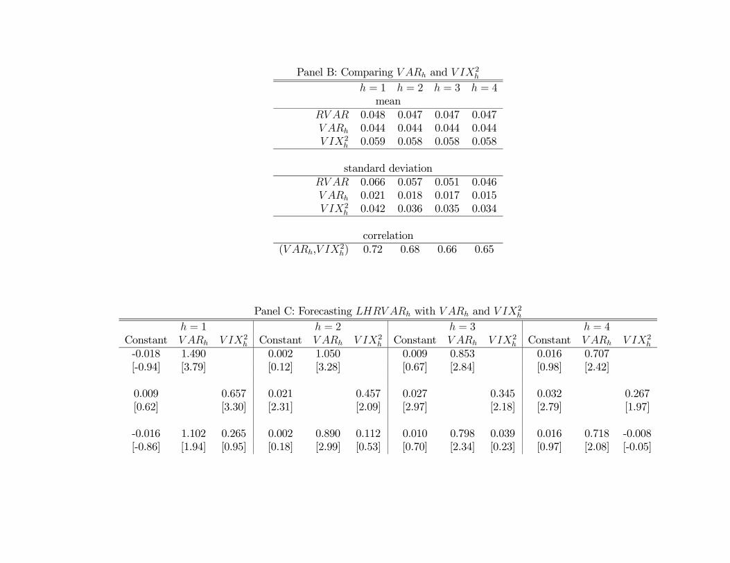
Panel B: Comparing and 2

= 1 = 2 = 3 = 4mean

0.048 0.047 0.047 0.047 0.044 0.044 0.044 0.044 2

0.059 0.058 0.058 0.058

standard deviation 0.066 0.057 0.051 0.046 0.021 0.018 0.017 0.015 2

0.042 0.036 0.035 0.034

correlation( , 2

) 0.72 0.68 0.66 0.65

Panel C: Forecasting with and 2

= 1 = 2 = 3 = 4Constant 2

Constant 2 Constant 2

Constant 2

-0.018 1.490 0.002 1.050 0.009 0.853 0.016 0.707[-0.94] [3.79] [0.12] [3.28] [0.67] [2.84] [0.98] [2.42]

0.009 0.657 0.021 0.457 0.027 0.345 0.032 0.267[0.62] [3.30] [2.31] [2.09] [2.97] [2.18] [2.79] [1.97]

-0.016 1.102 0.265 0.002 0.890 0.112 0.010 0.798 0.039 0.016 0.718 -0.008[-0.86] [1.94] [0.95] [0.18] [2.99] [0.53] [0.70] [2.34] [0.23] [0.97] [2.08] [-0.05]

Table 5: Cash-flow, Discount-rate, and Variance Betas in the Early SampleThe table shows the estimated cash-flow (β̂CF ), discount-rate (β̂DR), and variance betas(β̂V ) for the 25 ME- and BE/ME-sorted portfolios (Panel A) and six risk-sorted portfolios(Panel B). “Growth”denotes the lowest BE/ME, “Value”the highest BE/ME, “Small”thelowest ME, and "Large" the highest ME stocks. b̂∆V AR and b̂rM are past return-loadings onthe weighted sum of changes in the VAR state variables, where the weights are accordingto λV as estimated in Table 3, and on the market-return shock. “Diff.” is the differencebetween the extreme cells. Bootstrapped standard errors [in brackets] are conditional on theestimated news series. Estimates are based on quarterly data for the 1931:3-1963:2 periodusing weighted least squares where the weights are the same as those used to estimate theVAR.

Panel A: 25 ME- and BE/ME-sorted portfolios

β̂CF Growth 2 3 4 Value DiffSmall 0.44 [0.13] 0.41 [0.11] 0.39 [0.10] 0.41 [0.10] 0.43 [0.10] -0.01 [0.06]2 0.29 [0.07] 0.33 [0.09] 0.33 [0.08] 0.36 [0.08] 0.41 [0.10] 0.12 [0.04]3 0.29 [0.08] 0.27 [0.08] 0.32 [0.09] 0.32 [0.08] 0.44 [0.12] 0.15 [0.05]4 0.25 [0.07] 0.26 [0.07] 0.30 [0.08] 0.33 [0.08] 0.43 [0.11] 0.18 [0.05]Large 0.22 [0.07] 0.22 [0.07] 0.25 [0.08] 0.32 [0.10] 0.38 [0.29] 0.16 [0.04]Diff -0.22 [0.07] -0.19 [0.05] -0.14 [0.04] -0.09 [0.03] -0.05 [0.03]

β̂DR Growth 2 3 4 Value DiffSmall 1.13 [0.15] 1.12 [0.16] 1.09 [0.17] 1.07 [0.16] 1.05 [0.16] -0.07 [0.07]2 0.85 [0.11] 0.94 [0.14] 0.91 [0.14] 0.92 [0.16] 1.06 [0.13] 0.21 [0.08]3 0.86 [0.13] 0.77 [0.09] 0.88 [0.11] 0.86 [0.11] 1.07 [0.15] 0.21 [0.09]4 0.66 [0.07] 0.75 [0.10] 0.78 [0.09] 0.85 [0.14] 1.11 [0.16] 0.44 [0.13]Large 0.67 [0.08] 0.63 [0.08] 0.69 [0.11] 0.89 [0.15] 0.89 [0.12] 0.22 [0.13]Diff -0.45 [0.14] -0.49 [0.11] -0.41 [0.16] -0.18 [0.13] -0.17 [0.08]

β̂V Growth 2 3 4 Value DiffSmall -0.08 [0.05] -0.09 [0.04] -0.10 [0.04] -0.09 [0.04] -0.10 [0.04] -0.02 [0.02]2 -0.05 [0.03] -0.05 [0.03] -0.06 [0.03] -0.07 [0.03] -0.09 [0.04] -0.05 [0.02]3 -0.05 [0.03] -0.03 [0.02] -0.05 [0.03] -0.06 [0.03] -0.10 [0.04] -0.05 [0.02]4 -0.01 [0.02] -0.03 [0.02] -0.04 [0.03] -0.06 [0.04] -0.10 [0.05] -0.09 [0.03]Large -0.01 [0.02] -0.02 [0.02] -0.05 [0.04] -0.08 [0.04] -0.07 [0.03] -0.06 [0.03]Diff 0.07 [0.04] 0.07 [0.02] 0.04 [0.02] 0.01 [0.02] 0.02 [0.02]

61

Panel B: 6 risk-sorted portfolios

β̂CF Lo b̂rM 2 Hi b̂rM DiffLo b̂V AR 0.22 [0.07] 0.33 [0.09] 0.43 [0.12] 0.21 [0.05]Hi b̂V AR 0.18 [0.06] 0.26 [0.08] 0.36 [0.10] 0.17 [0.05]Diff -0.04 [0.02] -0.07 [0.03] -0.08 [0.02]

β̂DR Lo b̂rM 2 Hi b̂rM DiffLo b̂V AR 0.61 [0.07] 0.87 [0.11] 1.09 [0.14] 0.48 [0.09]Hi b̂V AR 0.55 [0.06] 0.76 [0.09] 0.95 [0.11] 0.40 [0.07]Diff -0.07 [0.04] -0.12 [0.06] -0.14 [0.05]

β̂V Lo b̂rM 2 Hi b̂rM DiffLo b̂V AR -0.02 [0.02] -0.05 [0.03] -0.07 [0.04] -0.05 [0.02]Hi b̂V AR -0.01 [0.02] -0.02 [0.02] -0.04 [0.03] -0.03 [0.02]Diff 0.01 [0.01] 0.03 [0.02] 0.03 [0.01]

62

Table 6: Cash-flow, Discount-rate, and Variance Betas in the Modern SampleThe table shows the estimated cash-flow (β̂CF ), discount-rate (β̂DR), and variance betas (β̂V )for the 25 ME- and BE/ME-sorted portfolios (Panel A); six risk-sorted portfolios (Panel B);18 BE/ME, IVol, and β̂∆V AR-sorted portfolios (Panel C); the S&P 100 index straddle port-folio (STRADDLE), the Fama-French factors RMRF , SMB, HML, high yield (HY RET )and investment grade (IGRET ) bond portfolios (Panel D); five interest-rate-sorted portfo-lios of Lustig, Roussanov, and Verdelhan (2011) (Panel E); and 12 VIX Forward positions(delevered twenty-fold) (Panel F). “Growth”denotes the lowest BE/ME, “Value”the highestBE/ME, “Small” the lowest ME, and "Large" the highest ME stocks. b̂∆V AR and b̂rM arepast return-loadings on the weighted sum of changes in the VAR state variables, where theweights are according to λV as estimated in Table 3, and on the market-return shock. “Diff.”is the difference between the extreme cells. In Panel C, P1 is the composite portfolio that islong the equal-weight average of the value portfolios and is short the equal-weight averageof the growth portfolios. P2 is the composite portfolio that is long the high idiosyncraticportfolio and short the low idiosyncratic portfolio for either the growth subset or the valuesubset. P3 is the portfolio that is long the equal-weight average of the high β̂∆V AR portfoliosand is short the equal-weight average of the low β̂∆V AR portfolios. Bootstrapped standarderrors [in brackets] are conditional on the estimated news series. Estimates are based onquarterly data for the 1963:3-2011:4 period in Panels A, B and C, the 1986:1-2011:4 periodin Panel D, the 1984:1-2010:1 period in Panel E, and the 1998:4-2011:4 period in Panel Fusing weighted least squares where the weights are the same as those used to estimate theVAR.

Panel A: 25 ME- and BE/ME-sorted portfolios

β̂CF Growth 2 3 4 Value DiffSmall 0.23 [0.06] 0.24 [0.05] 0.24 [0.04] 0.23 [0.04] 0.26 [0.05] 0.03 [0.03]2 0.22 [0.05] 0.22 [0.04] 0.24 [0.04] 0.24 [0.04] 0.26 [0.05] 0.04 [0.03]3 0.20 [0.05] 0.22 [0.04] 0.22 [0.04] 0.23 [0.04] 0.24 [0.04] 0.05 [0.03]4 0.19 [0.04] 0.21 [0.04] 0.22 [0.04] 0.22 [0.04] 0.24 [0.04] 0.05 [0.03]Large 0.13 [0.03] 0.17 [0.03] 0.16 [0.03] 0.17 [0.03] 0.19 [0.04] 0.05 [0.03]Diff -0.10 [0.04] -0.07 [0.03] -0.08 [0.02] -0.06 [0.02] -0.07 [0.03]

β̂DR Growth 2 3 4 Value DiffSmall 1.31 [0.10] 1.06 [0.08] 0.89 [0.07] 0.83 [0.07] 0.87 [0.09] -0.44 [0.08]2 1.21 [0.09] 0.97 [0.07] 0.85 [0.06] 0.76 [0.07] 0.80 [0.08] -0.42 [0.08]3 1.14 [0.07] 0.89 [0.05] 0.77 [0.06] 0.72 [0.06] 0.72 [0.07] -0.42 [0.08]4 1.03 [0.06] 0.85 [0.05] 0.74 [0.06] 0.72 [0.06] 0.75 [0.07] -0.28 [0.08]Large 0.84 [0.05] 0.71 [0.04] 0.60 [0.05] 0.59 [0.06] 0.64 [0.06] -0.20 [0.06]Diff -0.46 [0.10] -0.35 [0.08] -0.29 [0.06] -0.24 [0.07] -0.23 [0.08]

β̂V Growth 2 3 4 Value DiffSmall 0.18 [0.07] 0.12 [0.06] 0.08 [0.06] 0.07 [0.05] 0.03 [0.07] -0.15 [0.03]2 0.19 [0.07] 0.12 [0.06] 0.08 [0.05] 0.06 [0.06] 0.04 [0.06] -0.15 [0.03]3 0.19 [0.06] 0.11 [0.05] 0.08 [0.05] 0.04 [0.06] 0.06 [0.04] -0.13 [0.03]4 0.17 [0.06] 0.11 [0.05] 0.06 [0.06] 0.05 [0.06] 0.04 [0.06] -0.13 [0.03]Large 0.13 [0.05] 0.10 [0.04] 0.06 [0.04] 0.04 [0.05] 0.04 [0.05] -0.09 [0.02]Diff -0.05 [0.03] -0.02 [0.03] -0.03 [0.02] -0.03 [0.02] 0.01 [0.03]

Panel B: 6 risk-sorted portfolios

β̂CF Lo b̂rM 2 Hi b̂rM DiffLo b̂V AR 0.16 [0.03] 0.17 [0.03] 0.25 [0.05] 0.08 [0.04]Hi b̂V AR 0.15 [0.02] 0.17 [0.04] 0.23 [0.05] 0.08 [0.04]Diff -0.01 [0.02] 0.00 [0.02] -0.01 [0.02]

β̂DR Lo b̂rM 2 Hi b̂rM DiffLo b̂V AR 0.55 [0.05] 0.71 [0.06] 1.11 [0.09] 0.56 [0.08]Hi b̂V AR 0.73 [0.06] 0.95 [0.05] 1.27 [0.09] 0.54 [0.11]Diff 0.18 [0.07] 0.24 [0.07] 0.16 [0.06]

β̂V Lo b̂rM 2 Hi b̂rM DiffLo b̂V AR 0.06 [0.05] 0.08 [0.05] 0.12 [0.07] 0.07 [0.03]Hi b̂V AR 0.11 [0.04] 0.16 [0.04] 0.18 [0.07] 0.07 [0.04]Diff 0.05 [0.02] 0.08 [0.02] 0.06 [0.02]

64

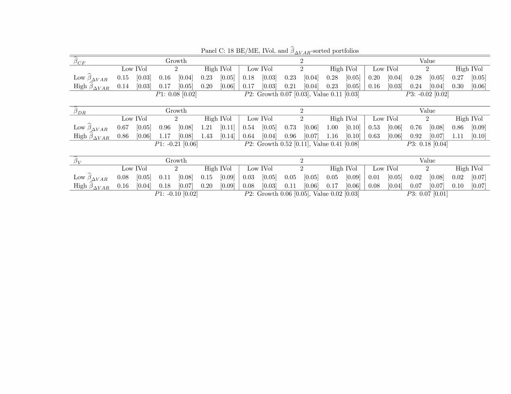
Panel C: 18 BE/ME, IVol, and b∆ -sorted portfoliosb Growth 2 ValueLow IVol 2 High IVol Low IVol 2 High IVol Low IVol 2 High IVol

Low b∆ 0.15 [0.03] 0.16 [0.04] 0.23 [0.05] 0.18 [0.03] 0.23 [0.04] 0.28 [0.05] 0.20 [0.04] 0.28 [0.05] 0.27 [0.05]High b∆ 0.14 [0.03] 0.17 [0.05] 0.20 [0.06] 0.17 [0.03] 0.21 [0.04] 0.23 [0.05] 0.16 [0.03] 0.24 [0.04] 0.30 [0.06]

1: 0.08 [0.02] 2: Growth 0.07 [0.03], Value 0.11 [0.03] 3: -0.02 [0.02]

b Growth 2 ValueLow IVol 2 High IVol Low IVol 2 High IVol Low IVol 2 High IVol

Low b∆ 0.67 [0.05] 0.96 [0.08] 1.21 [0.11] 0.54 [0.05] 0.73 [0.06] 1.00 [0.10] 0.53 [0.06] 0.76 [0.08] 0.86 [0.09]High b∆ 0.86 [0.06] 1.17 [0.08] 1.43 [0.14] 0.64 [0.04] 0.96 [0.07] 1.16 [0.10] 0.63 [0.06] 0.92 [0.07] 1.11 [0.10]

1: -0.21 [0.06] 2: Growth 0.52 [0.11], Value 0.41 [0.08] 3: 0.18 [0.04]

b Growth 2 ValueLow IVol 2 High IVol Low IVol 2 High IVol Low IVol 2 High IVol

Low b∆ 0.08 [0.05] 0.11 [0.08] 0.15 [0.09] 0.03 [0.05] 0.05 [0.05] 0.05 [0.09] 0.01 [0.05] 0.02 [0.08] 0.02 [0.07]High b∆ 0.16 [0.04] 0.18 [0.07] 0.20 [0.09] 0.08 [0.03] 0.11 [0.06] 0.17 [0.06] 0.08 [0.04] 0.07 [0.07] 0.10 [0.07]

1: -0.10 [0.02] 2: Growth 0.06 [0.05], Value 0.02 [0.03] 3: 0.07 [0.01]

Panel D: Option, equity, and bond portfoliosSTRADDLE RMRF SMB HML HY RET IGRET

β̂CF -0.39 [0.27] 0.18 [0.05] 0.04 [0.02] 0.05 [0.03] 0.06 [0.02] 0.00 [0.01]

β̂DR -1.71 [0.47] 0.81 [0.06] 0.19 [0.05] -0.25 [0.09] 0.26 [0.07] 0.03 [0.03]

β̂V 0.38 [0.21] -0.00 [0.07] -0.00 [0.02] -0.12 [0.03] -0.05 [0.05] 0.01 [0.01]

Panel E: Currency portfoliosLow r∗ 2 3 4 High r∗ Diff

β̂CF 0.00 [0.02] -0.03 [0.02] 0.00 [0.02] 0.02 [0.02] 0.02 [0.02] 0.02 [0.02]

β̂DR -0.16 [0.08] -0.08 [0.10] -0.09 [0.07] 0.01 [0.08] -0.01 [0.08] 0.15 [0.09]

β̂V 0.01 [0.03] -0.04 [0.04] -0.03 [0.02] -0.02 [0.03] -0.05 [0.04] -0.07 [0.06]

Panel F: V IX2 Forward PositionsMaturity β̂CF β̂DR β̂V

1 -0.11 [0.04] -0.33 [0.19] 0.21 [0.14]2 -0.06 [0.03] -0.21 [0.09] 0.11 [0.08]3 -0.03 [0.02] -0.13 [0.06] 0.07 [0.05]4 -0.03 [0.02] -0.11 [0.06] 0.06 [0.04]5 -0.02 [0.01] -0.14 [0.11] 0.10 [0.09]6 -0.03 [0.01] -0.04 [0.03] 0.04 [0.01]7 -0.01 [0.01] -0.06 [0.04] 0.04 [0.02]8 -0.03 [0.01] -0.06 [0.04] 0.04 [0.02]9 -0.04 [0.02] -0.02 [0.04] 0.04 [0.02]10 -0.03 [0.03] -0.02 [0.04] 0.04 [0.02]11 -0.01 [0.01] 0.00 [0.04] 0.04 [0.02]12 0.00 [0.02] 0.00 [0.04] 0.03 [0.02]12-1 0.12 [0.05] 0.38 [0.22] -0.22 [0.17]

66

Table 7: Asset Pricing Tests for the Early SampleThe table shows the premia estimated from the 1931:3-1963:2 sample for the CAPM, the 2-beta ICAPM, the 3-beta volatilityICAPM, a factor model where only the b premium is restricted, and an unrestricted factor model. The test assets are the25 ME- and BE/ME-sorted portfolios. The first column per model constrains the zero-beta rate () to equal the risk-free rate( ) while the second column allows to be a free parameter. Estimates are from a cross-sectional regression of average simple

excess test-asset returns (quarterly in fractions) on an intercept and estimated cash-flow (b ), discount-rate (b), and variancebetas (b ). Standard errors and critical values [A] are conditional on the estimated news series and (B) incorporate full estimationuncertainty of the news terms. The test rejects if the pricing error is higher than the listed 5 percent critical value.Parameter CAPM 2-beta ICAPM 3-beta ICAPM Constrained Unrestricted less (0) 0 -0.002 0 0.001 0 0.002 0 0.015 0 0.023% per annum 0% -0.90% 0% 0.21% 0% 0.86% 0% 6.08% 0% 8.98%Std. err. A 0 [0.016] 0 [0.014] 0 [0.011] 0 [0.018] 0 [0.022]Std. err. B 0 (0.016) 0 (0.016) 0 (0.014) 0 (0.017) 0 (0.020)b premium (1) 0.038 0.040 0.096 0.094 0.086 0.081 0.081 0.009 0.075 0.057% per annum 15.11% 15.82% 38.33% 37.74% 34.30% 32.52% 32.48% 3.67% 29.88% 22.69%Std. err. A [0.015] [0.024] [0.054] [0.079] [0.038] [0.048] [0.062] [0.106] [0.125] [0.129]Std. err. B (0.015) (0.024) (0.142) (0.111) (0.072) (0.082) (0.101) (0.118) (0.129) (0.139)b premium (2) 0.038 0.040 0.016 0.016 0.016 0.016 0.016 0.016 0.018 -0.012% per annum 15.11% 15.82% 6.40% 6.40% 6.40% 6.40% 6.40% 6.40% 7.28% -4.78%Std. err. A [0.015] [0.024] [0.004] [0.004] [0.004] [0.004] [0.004] [0.004] [0.050] [0.064]Std. err. B (0.015) (0.024) (0.004) (0.004) (0.004) (0.004) (0.004) (0.004) (0.075) (0.089)b premium (3) -0.053 -0.045 -0.077 -0.227 -0.080 -0.258% per annum -21.27% -17.97% -30.67% -90.62% -31.96% -103.04%Std. err. A [0.048] [0.061] [0.186] [0.237] [0.210] [0.304]Std. err. B (0.146) (0.146) (0.549) (0.558) (0.684) (0.782)c2 53.01% 53.12% 54.72% 54.73% 55.65% 55.83% 55.74% 57.94% 55.75% 58.87%Pricing error 0.024 0.023 0.022 0.022 0.020 0.021 0.020 0.022 0.020 0.0235% critic. val. A [0.062] [0.031] [0.058] [0.038] [0.065] [0.044] [0.043] [0.038] [0.037] [0.038]5% critic. val. B (0.062) (0.031) (0.097) (0.046) (0.179) (0.052) (0.049) (0.040) (0.037) (0.042)Implied 2.4 2.5 6.0 5.9 5.4 5.1 N/A N/A N/A N/AImplied N/A N/A N/A N/A 6.7 5.6 N/A N/A N/A N/A

Table 8: Asset Pricing Tests for the Modern SampleThe table shows the premia estimated from the 1963:3-2011:4 sample for the CAPM, the 2-beta ICAPM, the 3-beta volatilityICAPM, a factor model where only the b premium is restricted, and an unrestricted factor model. The test assets are the25 ME- and BE/ME-sorted portfolios. The first column per model constrains the zero-beta rate () to equal the risk-free rate( ) while the second column allows to be a free parameter. Estimates are from a cross-sectional regression of average simple

excess test-asset returns (quarterly in fractions) on an intercept and estimated cash-flow (b ), discount-rate (b), and variancebetas (b ). Standard errors and critical values [A] are conditional on the estimated news series and (B) incorporate full estimationuncertainty of the news terms. The test rejects if the pricing error is higher than the listed 5 percent critical value.Parameter CAPM 2-beta ICAPM 3-beta ICAPM Constrained Unrestricted less (0) 0 0.027 0 -0.019 0 0.011 0 -0.004 0 -0.005% per annum 0% 10.62% 0% -7.71% 0% 4.50% 0% -1.66% 0% -2.00%Std. err. A 0 [0.014] 0 [0.013] 0 [0.012] 0 [0.013] 0 [0.013]Std. err. B 0 (0.014) 0 (0.019) 0 (0.015) 0 (0.015) 0 (0.015)b premium (1) 0.020 -0.004 0.074 0.161 0.047 0.054 0.112 0.128 0.175 0.199% per annum 7.98% -1.67% 29.41% 64.39% 18.78% 21.49% 44.65% 51.35% 70.18% 79.55%Std. err. A [0.010] [0.019] [0.047] [0.070] [0.024] [0.013] [0.050] [0.071] [0.070] [0.084]Std. err. B (0.010) (0.019) (0.087) (0.113) (0.040) (0.053) (0.114) (0.116) (0.124) (0.126)b premium (2) 0.020 -0.004 0.008 0.008 0.008 0.008 0.008 0.008 -0.018 -0.020% per annum 7.98% -1.67% 3.11% 3.11% 3.11% 3.11% 3.11% 3.11% -7.30% -7.83%Std. err. A [0.010] [0.019] [0.002] [0.002] [0.002] [0.002] [0.002] [0.002] [0.023] [0.025]Std. err. B (0.010) (0.019) (0.002) (0.002) (0.002) (0.002) (0.002) (0.002) (0.054) (0.055)b premium (3) -0.039 -0.081 -0.094 -0.089 -0.002 0.009% per annum -15.51% -32.47% -37.65% -35.60% -0.72% 3.62%Std. err. A [0.039] [0.024] [0.063] [0.069] [0.092] [0.094]Std. err. B (0.091) (0.151) (0.356) (0.349) (0.399) (0.387)c2 -36.51% 5.22% 25.10% 39.97% -108.63% 62.74% 73.90% 74.45% 76.46% 77.25%Pricing error 0.110 0.107 0.058 0.042 0.210 0.042 0.027 0.025 0.026 0.0235% critic. val. A [0.050] [0.034] [0.061] [0.056] [0.503] [0.101] [0.051] [0.037] [0.046] [0.031]5% critic. val. B (0.049) (0.033) (0.096) (0.083) (0.492) (0.119) (0.104) (0.078) (0.065) (0.049)Implied 2.6 -0.5 9.5 20.7 6.0 6.9 N/A N/A N/A N/AImplied N/A N/A N/A N/A 10.0 20.9 N/A N/A N/A N/A

Table 9: Asset Pricing Tests for the Modern Sample: Various Sets of Test AssetsThe table shows the premia estimated from the 1963:3-2011:4 sample for the CAPM, the 2-beta ICAPM, and the 3-beta volatilityICAPM. Test assets vary across the table and in Panel A are as follows: “Risk-sorted” are six ME- and BE/ME-sorted portfolios andsix risk-sorted portfolios, “Idiosyncratic Volatility” are 18 BE/ME, IVol, and b∆ -sorted portfolios, and “Straddle, Equity, andBonds” are the three equity factors of Fama and French (1993), the returns on high yield and investment grade bond portfolios, andthe S&P 100 index straddle return from Coval and Shumway (2001). In Panel B, the test assets are “Carry Trade”, the five interest-rate-sorted currency portfolios from developed countries of Lustig, Roussanov, and Verdelhan (2011), and “Variance Forward”,twelve variance forward positions of maturities from one month to one year. Estimates are from a cross-sectional regression ofaverage simple excess test-asset returns (quarterly in fractions) on an intercept and estimated cash-flow (b ), discount-rate (b),and variance betas (b ). The constrained 2 row reports the 2 when model parameters, including , are constrained to be thesame as in Table 8. Standard errors and critical values [A] are conditional on the estimated news series and (B) incorporate fullestimation uncertainty of the news terms. The test rejects if the pricing error is higher than the listed 5 percent critical value.

Panel A Risk-sorted Idiosycratic Volatility Straddle, Equity, and Bonds2-beta 3-beta 2-beta 3-beta 2-beta 3-beta

Parameter CAPM ICAPM ICAPM CAPM ICAPM ICAPM CAPM ICAPM ICAPM less (0) 0.017 -0.004 0.009 0.032 -0.013 0.007 -0.002 -0.004 -0.002% per annum 6.60% -1.74% 3.50% 12.83% -5.34% 2.79% -0.61% -1.77% -0.85%Std. err. A [0.009] [0.011] [0.011] [0.012] [0.013] [0.012] [0.002] [0.003] [0.003]Std. err. B (0.009) (0.013) (0.011) (0.012) (0.019) (0.013) (0.002) (0.003) (0.003)b premium (1) 0.001 0.078 0.054 -0.013 0.114 0.054 0.025 0.144 0.055% per annum 0.44% 31.12% 21.49% -5.13% 45.69% 21.49% 9.85% 57.46% 22.11%Std. err. A [0.014] [0.071] [0.022] [0.017] [0.059] [0.015] [0.010] [0.070] [0.012]Std. err. B (0.014) (0.102) (0.050) (0.016) (0.120) (0.051) (0.010) (0.082) (0.034)b premium (2) 0.001 0.008 0.008 -0.013 0.008 0.008 0.025 0.008 0.008% per annum 0.44% 3.11% 3.11% -5.13% 3.11% 3.11% 9.85% 3.20% 3.20%Std. err. A [0.014] [0.002] [0.002] [0.017] [0.002] [0.002] [0.010] [0.001] [0.001]Std. err. B (0.014) (0.002) (0.002) (0.016) (0.002) (0.002) (0.010) (0.001) (0.001)b premium (3) -0.081 -0.081 -0.084% per annum -32.47% -32.47% -33.39%Std. err. A [0.034] [0.028] [0.023]Std. err. B (0.131) (0.145) (0.106)c2 8.49% 17.89% 68.23% 14.05% 11.33% 48.62% 50.68% 65.87% 71.24%constrained c2 -29.21% -6.62% 57.17% -2.05% -4.38% 35.02% -159.21% 5.84% 16.52%Pricing error 0.041 0.032 0.016 0.118 0.118 0.060 0.349 0.344 0.2925% critic. val. A [0.022] [0.029] [0.074] [0.040] [0.058] [0.105] [0.101] [0.138] [0.178]5% critic. val. B (0.022) (0.028) (0.077) (0.040) (0.059) (0.121) (0.100) (0.194) (0.181)Implied 0.1 10.0 6.9 -1.7 14.7 6.9 3.1 18.0 6.9Implied N/A N/A 20.9 N/A N/A 20.9 N/A N/A 20.9

Panel B Carry trade Variance Forwards2-beta 3-beta 2-beta 3-beta

Parameter CAPM ICAPM ICAPM CAPM ICAPM ICAPM less (0) 0.007 0.005 0.003 0.010 0.010 0.012% per annum 2.79% 2.17% 1.32% 3.95% 4.06% 4.60%Std. err. A [0.005] [0.005] [0.004] [0.003] [0.004] [0.004]Std. err. B (0.005) (0.005) (0.005) (0.003) (0.004) (0.004)b premium (1) 0.030 0.107 0.052 0.071 0.256 0.070% per annum 12.17% 42.85% 20.72% 28.34% 102.29% 28.10%Std. err. A [0.011] [0.104] [0.020] [0.042] [0.135] [0.020]Std. err. B (0.011) (0.083) (0.031) (0.042) (0.147) (0.051)b premium (2) 0.030 0.008 0.008 0.071 0.010 0.010% per annum 12.17% 3.00% 3.00% 28.34% 4.07% 4.07%Std. err. A [0.011] [0.001] [0.001] [0.042] [0.002] [0.002]Std. err. B (0.011) (0.001) (0.001) (0.042) (0.002) (0.002)b premium (3) 0.0000 0.0000 -0.078 0.0000 0.0000 -0.106% per annum 0.00% 0.00% -31.31% 0.00% 0.00% -42.45%Std. err. A [0.0000] [0.0000] [0.029] [0.0000] [0.0000] [0.037]Std. err. B (0.0000) (0.0000) (0.064) (0.0000) (0.0000) (0.172)c2 59.41% 59.67% 81.59% 83.49% 75.91% 83.61%constrained c2 -4190.89% -5329.39% -476.65% -738.66% -768.78% 83.53%Pricing error 0.008 0.008 0.004 0.209 0.341 0.1705% critic. val. A [0.030] [0.042] [0.079] [0.679] [0.757] [1.226]5% critic. val. B (0.030) (0.044) (0.076) (0.668) (0.779) (1.055)Implied 4.1 14.3 6.9 7.0 25.2 6.9Implied N/A N/A 20.9 N/A N/A 20.9

70

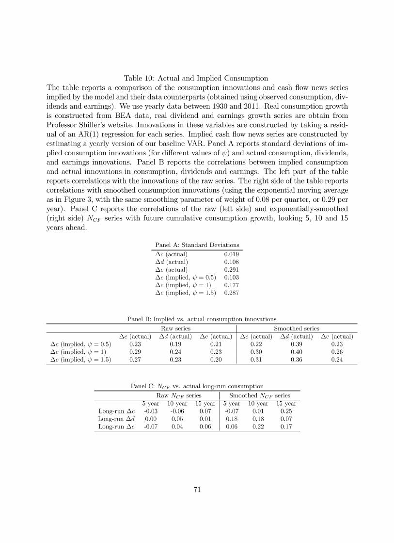
Table 10: Actual and Implied ConsumptionThe table reports a comparison of the consumption innovations and cash flow news seriesimplied by the model and their data counterparts (obtained using observed consumption, div-idends and earnings). We use yearly data between 1930 and 2011. Real consumption growthis constructed from BEA data, real dividend and earnings growth series are obtain fromProfessor Shiller’s website. Innovations in these variables are constructed by taking a resid-ual of an AR(1) regression for each series. Implied cash flow news series are constructed byestimating a yearly version of our baseline VAR. Panel A reports standard deviations of im-plied consumption innovations (for different values of ψ) and actual consumption, dividends,and earnings innovations. Panel B reports the correlations between implied consumptionand actual innovations in consumption, dividends and earnings. The left part of the tablereports correlations with the innovations of the raw series. The right side of the table reportscorrelations with smoothed consumption innovations (using the exponential moving averageas in Figure 3, with the same smoothing parameter of weight of 0.08 per quarter, or 0.29 peryear). Panel C reports the correlations of the raw (left side) and exponentially-smoothed(right side) NCF series with future cumulative consumption growth, looking 5, 10 and 15years ahead.

Panel A: Standard Deviations

∆c (actual) 0.019∆d (actual) 0.108∆e (actual) 0.291∆c (implied, ψ = 0.5) 0.103∆c (implied, ψ = 1) 0.177∆c (implied, ψ = 1.5) 0.287

Panel B: Implied vs. actual consumption innovations

Raw series Smoothed series∆c (actual) ∆d (actual) ∆e (actual) ∆c (actual) ∆d (actual) ∆e (actual)

∆c (implied, ψ = 0.5) 0.23 0.19 0.21 0.22 0.39 0.23∆c (implied, ψ = 1) 0.29 0.24 0.23 0.30 0.40 0.26∆c (implied, ψ = 1.5) 0.27 0.23 0.20 0.31 0.36 0.24

Panel C: NCF vs. actual long-run consumption

Raw NCF series Smoothed NCF series5-year 10-year 15-year 5-year 10-year 15-year

Long-run ∆c -0.03 -0.06 0.07 -0.07 0.01 0.25Long-run ∆d 0.00 0.05 0.01 0.18 0.18 0.07Long-run ∆e -0.07 0.04 0.06 0.06 0.22 0.17

71

Table 11: RobustnessThe table provides a variety of robustness tests. When appropriate, the baseline modelappears in bold font. Panel A reports the results when only a subset of state variables fromthe baseline VAR (D ≡ DEF , T ≡ TERM , V ≡ V S, P ≡ PE) are used to forecast returnsand realized variance. Panel B reports the results when different estimation techniquesare used. Panel C reports results as we change the estimate of realized variance. PanelD reports the results when other state variables either replace or are added to the VAR.These variables include the log real PE ratio (PERe al), the log price-dividend ratio (PD),log inflation (INFL), CAY , the quarterly FIGARCH variance forecast (FIG), and theterm spread volatility (TY V ol). Panel E reports the modern-period results when out-of-sample versions of the model’s news terms are used in the pricing tests. Panel F reportsresults using delevered market portfolios. Panel G reports results when the excess zero-beta rate is varied from 40 to 86 basis points per quarter. Panel H reports the componentsof RMRF and HML’s β̂V by re-estimating β̂V using each component of e2′λV . Panel Ialso reports simple loadings of RMRF and HML on RV AR and the 15-year FIGARCHvariance forecast. Panel J reports time-series regressions explaining HML with the threenews terms described in Table 3.

72

Panel A: Results Using Various Subsets of the Baseline VAR (rM and RV AR always included)None D D/T/V ALL P/D/V P/D P

γ̂Max 4.5 3.2 3.1 6.9 6.7 8.9 14.9

Early Periodβ̂V

RMRF -0.03 -0.23 -0.20 -0.03 -0.03 -0.02 0.08SMB -0.01 -0.08 -0.07 -0.02 -0.02 -0.02 0.03HML 0.00 -0.12 -0.14 -0.06 -0.06 -0.04 0.06

Risk-free Rate ICAPMγ̂ 2.1 2.3 2.4 5.4 5.4 5.5 8.1ω̂ 2.0 2.5 3.2 6.7 6.9 5.3 12.3R̂2 51.35% 51.63% 53.78% 55.65% 55.63% 52.14% 42.27%

Zero-beta Rate ICAPMR̂zb less Rf -0.08% -0.20% -0.10% 0.21% 0.22% -0.10% 0.78%γ̂ 2.2 2.3 2.5 5.1 5.1 5.7 5.3ω̂ 2.1 2.8 3.4 5.6 5.8 5.7 4.4R̂2 51.36% 51.72% 53.81% 55.83% 55.82% 52.17% 44.61%

Modern Periodβ̂V

RMRF -0.11 -0.15 -0.07 0.10 0.11 0.07 0.00SMB -0.03 -0.05 -0.03 0.02 0.03 0.01 0.00HML 0.00 -0.01 -0.10 -0.11 -0.11 -0.05 -0.02

Risk-free Rate ICAPMγ̂ 2.3 2.3 2.6 6.0 5.6 8.6 6.15ω̂ 3.0 2.9 4.7 10.0 8.3 21.6 6.34R̂2 -37.26% -37.15% 1.71% -108.63% -136.46% -27.78% -43.34%

Zero-beta Rate ICAPMR̂zb less Rf 2.12% 2.09% -0.70% 1.12% 1.22% 0.45% 1.60%γ̂ 0.0 0.0 3.1 6.9 6.7 8.9 0.0ω̂ 1.3 1.1 12.6 20.9 19.4 28.3 0.2R̂2 5.04% 6.72% 21.89% 62.74% 57.42% 3.38% -0.48%

73

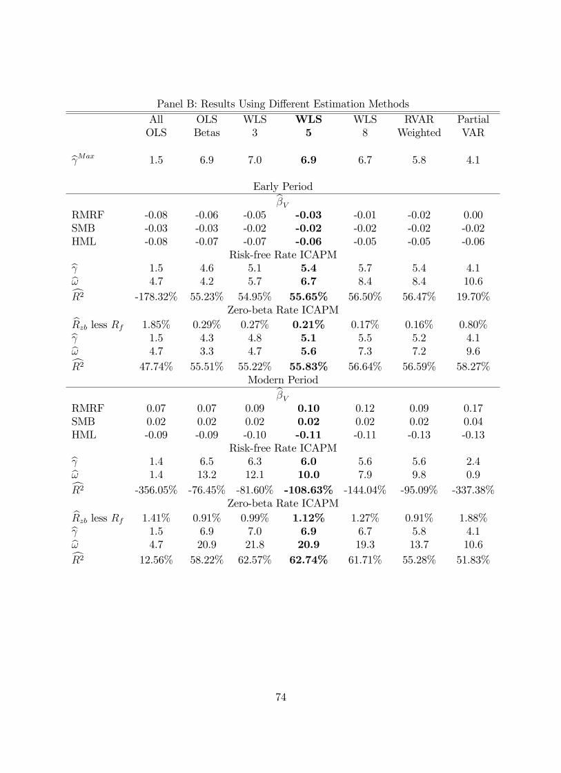
Panel B: Results Using Different Estimation MethodsAll OLS WLS WLS WLS RVAR PartialOLS Betas 3 5 8 Weighted VAR

γ̂Max 1.5 6.9 7.0 6.9 6.7 5.8 4.1

Early Periodβ̂V

RMRF -0.08 -0.06 -0.05 -0.03 -0.01 -0.02 0.00SMB -0.03 -0.03 -0.02 -0.02 -0.02 -0.02 -0.02HML -0.08 -0.07 -0.07 -0.06 -0.05 -0.05 -0.06

Risk-free Rate ICAPMγ̂ 1.5 4.6 5.1 5.4 5.7 5.4 4.1ω̂ 4.7 4.2 5.7 6.7 8.4 8.4 10.6R̂2 -178.32% 55.23% 54.95% 55.65% 56.50% 56.47% 19.70%

Zero-beta Rate ICAPMR̂zb less Rf 1.85% 0.29% 0.27% 0.21% 0.17% 0.16% 0.80%γ̂ 1.5 4.3 4.8 5.1 5.5 5.2 4.1ω̂ 4.7 3.3 4.7 5.6 7.3 7.2 9.6R̂2 47.74% 55.51% 55.22% 55.83% 56.64% 56.59% 58.27%

Modern Periodβ̂V

RMRF 0.07 0.07 0.09 0.10 0.12 0.09 0.17SMB 0.02 0.02 0.02 0.02 0.02 0.02 0.04HML -0.09 -0.09 -0.10 -0.11 -0.11 -0.13 -0.13

Risk-free Rate ICAPMγ̂ 1.4 6.5 6.3 6.0 5.6 5.6 2.4ω̂ 1.4 13.2 12.1 10.0 7.9 9.8 0.9R̂2 -356.05% -76.45% -81.60% -108.63% -144.04% -95.09% -337.38%

Zero-beta Rate ICAPMR̂zb less Rf 1.41% 0.91% 0.99% 1.12% 1.27% 0.91% 1.88%γ̂ 1.5 6.9 7.0 6.9 6.7 5.8 4.1ω̂ 4.7 20.9 21.8 20.9 19.3 13.7 10.6R̂2 12.56% 58.22% 62.57% 62.74% 61.71% 55.28% 51.83%

74

Panel C: Results Using Different Measures of Realized VarianceQuarterly Annual Quarterly Quarterly Annual AnnualVar Daily Var Daily Var Monthly Sum Monthly Var Monthly Sum Monthly

γ̂Max 6.9 5.8 5.1 5.1 6.2 5.5

Early Periodβ̂V

RMRF -0.03 0.21 -0.18 -0.24 0.12 0.19SMB -0.02 0.07 -0.08 -0.07 0.04 0.05HML -0.06 0.06 -0.14 -0.15 0.00 0.10

Risk-free Rate ICAPMγ̂ 5.4 3.7 4.0 4.2 5.5 4.6ω̂ 6.7 2.0 3.5 3.1 6.9 3.4R̂2 55.65% -991.53% 56.95% 53.85% -781.40% -887.87%

Zero-beta Rate ICAPMR̂zb less Rf 0.21% 3.68% 0.11% 0.19% 3.31% 3.51%γ̂ 5.1 1.5 3.9 4.1 3.7 2.7ω̂ 5.6 0.1 3.3 2.7 1.8 0.5R̂2 55.83% 16.70% 56.99% 53.96% 18.74% 17.89%

Modern Periodβ̂V

RMRF 0.10 0.12 0.03 -0.01 0.09 0.10SMB 0.02 -0.02 -0.01 -0.03 -0.03 -0.06HML -0.11 -0.06 -0.12 -0.14 -0.05 -0.06

Risk-free Rate ICAPMγ̂ 6.0 4.5 5.1 5.1 5.6 5.3ω̂ 10.0 3.9 11.6 8.7 7.1 6.1R̂2 -108.63% -361.48% -27.69% 2.44% -235.53% -229.17%

Zero-beta Rate ICAPMR̂zb less Rf 1.12% 1.83% 0.66% 0.49% 1.45% 1.35%γ̂ 6.9 5.8 5.1 5.1 6.2 5.5ω̂ 20.9 13.4 11.6 8.7 14.0 9.0R̂2 62.74% 62.14% 56.63% 49.08% 58.73% 54.42%

75

Panel D: Results Replacing/Adding Other State Variables to the VARPE PERe al PD INFL CAY FIG TY V OL

γ̂Max 6.9 8.8 4.5 9.0 14.7 5.4

Early Periodβ̂V

RMRF -0.03 0.01 -0.12 0.02 0.06 -0.03 -0.01SMB -0.02 -0.01 -0.05 -0.01 0.01 -0.02 -0.01HML -0.06 -0.04 -0.10 -0.03 0.00 -0.03 -0.04

Risk-free Rate ICAPMγ̂ 5.4 5.4 3.1 5.8 12.4 5.0 5.8ω̂ 6.7 4.3 2.9 5.1 26.8 8.0 8.4R̂2 55.65% 55.89% 57.77% 55.98% -1228.81% 56.57% 55.42%

Zero-beta Rate ICAPMR̂zb less Rf 0.21% -0.17% -0.15% -0.23% 2.19% 0.10% 0.22%γ̂ 5.1 5.7 3.2 6.2 14.7 4.9 5.4ω̂ 5.6 4.9 3.2 6.0 56.6 7.3 7.0R̂2 55.83% 55.97% 57.83% 56.13% 23.45% 56.60% 55.62%

Modern Periodβ̂V

RMRF 0.10 0.12 -0.01 0.13 0.06 0.09 0.10SMB 0.02 0.03 -0.01 0.03 0.02 0.03 0.02HML -0.11 -0.08 -0.09 -0.08 -0.05 -0.07 -0.11

Risk-free Rate ICAPMγ̂ 6.0 8.0 4.1 8.0 14.5 4.6 6.1ω̂ 10.0 13.4 8.3 12.8 48.3 5.7 10.3R̂2 -108.63% -32.02% 2.59% -38.01% 17.06% -183.16% -99.86%

Zero-beta Rate ICAPMR̂zb less Rf 1.12% 0.72% -0.36% 0.81% 0.35% 1.21% 1.10%γ̂ 6.9 8.8 4.5 9.0 14.7 5.4 6.9ω̂ 20.9 22.8 15.9 23.4 56.6 13.5 20.8R̂2 62.74% 26.08% 20.12% 31.92% 35.16% 41.44% 65.68%

76

Panel E: Modern Period PricingFull Sample Out of Sample

β̂VRMRF 0.10 -0.04SMB 0.02 -0.02HML -0.11 -0.10

Risk-free Rate ICAPMγ̂ 6.0 6.8ω̂ 10.0 20.7R̂2 -108.63% 52.09%

Zero-beta Rate ICAPMR̂zb less Rf 1.12% 0.22%γ̂ 6.9 6.9ω̂ 20.9 20.1R̂2 62.74% 59.92%

77

Panel F: Results Using delevered market portfoliosEquity % 100% 80% 60% 40%

γ̂Max 6.9 10.0 15.1 21.5

Early Periodβ̂V

RMRF -0.03 -0.03 -0.03 -0.02SMB -0.02 -0.02 -0.02 -0.02HML -0.06 -0.06 -0.05 -0.05

Risk-free Rate ICAPMγ̂ 5.36 7.96 12.24 18.84ω̂ 6.65 17.27 58.58 395.71R̂2 55.65% 55.45% 54.82% 53.25%

Zero-beta Rate ICAPMR̂zb less Rf 0.21% 0.31% 0.44% 0.71%γ̂ 5.08 7.41 11.19 16.73ω̂ 5.62 14.09 46.33 291.98R̂2 55.83% 55.86% 55.69% 55.88%

Modern Periodβ̂V

RMRF 0.10 0.10 0.10 0.08SMB 0.02 0.02 0.02 0.02HML -0.11 -0.11 -0.11 -0.09

Risk-free Rate ICAPMγ̂ 6.04 8.69 12.95 17.56ω̂ 9.97 22.70 68.78 329.06R̂2 -108.63% -120.66% -114.82% -180.16%

Zero-beta Rate ICAPMR̂zb less Rf 1.12% 1.19% 1.04% 1.11%γ̂ 6.91 9.99 14.51 18.44ω̂ 20.88 45.20 101.91 373.59R̂2 62.74% 64.59% 63.55% 55.91%

78

Panel G: Varying ρ and the Excess Zero-beta Rate in the Modern Period

ρ = 0.94

R̂zb less Rf 0.40% 0.50% 0.60% 0.70% 0.80% 0.91%γ̂ 6.7 6.8 6.9 7.0 7.0 7.1ω̂ 15.3 16.5 18.0 19.9 22.1 22.7R̂2 32.51% 44.22% 52.83% 58.84% 62.78% 64.21%Pricing error 0.062 0.051 0.044 0.039 0.038 0.038

ρ = 0.95

R̂zb less Rf 0.40% 0.50% 0.60% 0.70% 0.80% 1.12%γ̂ 6.3 6.3 6.5 6.6 6.7 6.9ω̂ 11.4 12.1 13.0 14.3 15.8 20.9R̂2 0.48% 18.27% 32.50% 43.46% 51.54% 62.74%Pricing error 0.094 0.076 0.062 0.052 0.046 0.042

ρ = 0.96

R̂zb less Rf 0.40% 0.50% 0.60% 0.70% 0.80% 1.35%γ̂ 5.7 5.8 5.9 6.0 6.1 6.7ω̂ 8.1 8.5 9.0 9.8 10.8 19.1R̂2 -42.66% -18.68% 1.56% 18.21% 31.48% 60.67%Pricing error 0.138 0.113 0.092 0.076 0.063 0.046

79

Panel H: Components of and Proxies for β̂VEarly Period

RMRF HMLWLS OLS WLS OLS

β̂V -0.03 -0.06 -0.06 -0.07β̂λ1V rM Shock 0.00 0.00 0.00 0.00β̂λ2V EV AR Shock -0.06 -0.05 -0.02 -0.03β̂λ3V PE Shock 0.14 0.14 0.06 0.08β̂λ4V TY Shock 0.00 0.00 0.00 0.00β̂λ5VDEF Shock -0.13 -0.13 -0.09 -0.09β̂λ6V V S Shock -0.02 -0.02 -0.02 -0.03β̂RV AR -0.01 1.50β̂FIGARCH 0.02 0.04

Modern PeriodRMRF HML

WLS OLS WLS OLSβ̂V 0.10 0.07 -0.11 -0.09β̂λ1V rM Shock 0.00 0.00 0.00 0.00β̂λ2V EV AR Shock -0.08 -0.07 -0.01 -0.01β̂λ3V PE Shock 0.14 0.14 -0.02 -0.02β̂λ4V TY Shock 0.00 0.00 0.00 0.00β̂λ5VDEF Shock -0.02 -0.02 -0.02 -0.01β̂λ6V V S Shock 0.03 0.03 -0.05 -0.05β̂RV AR -3.31 -0.51β̂FIGARCH -0.08 -0.01

80

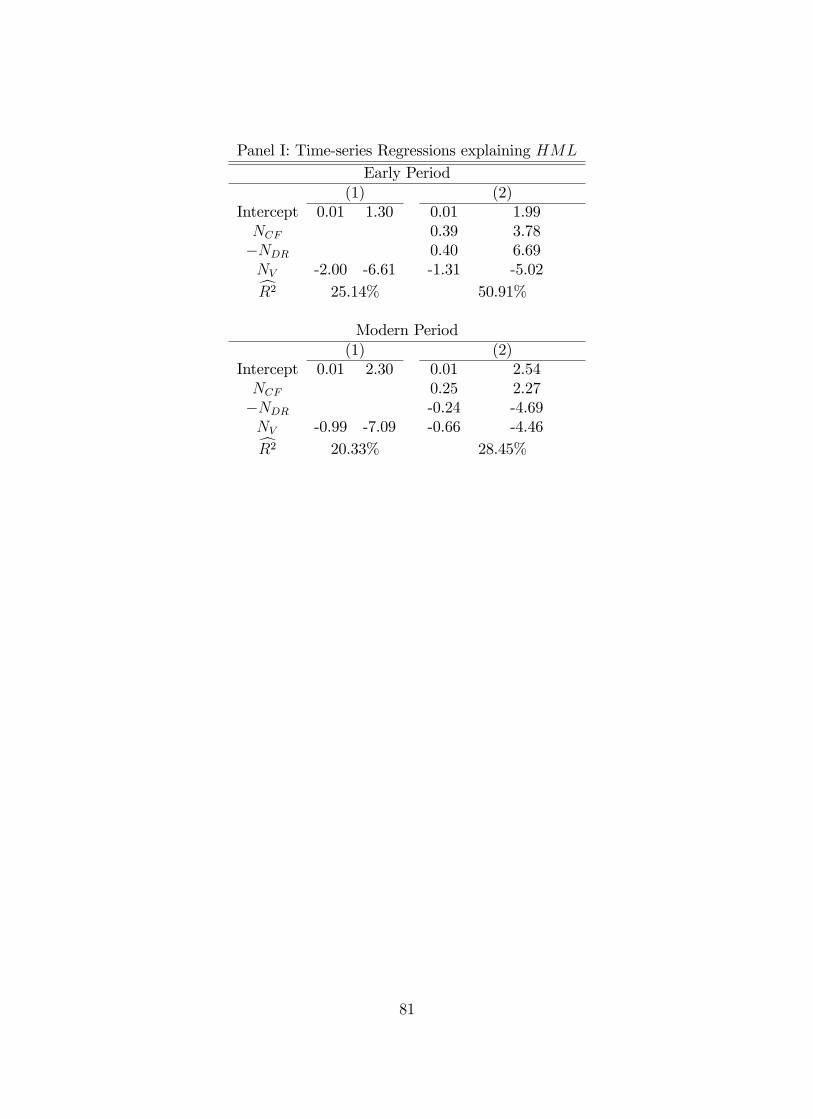
Panel I: Time-series Regressions explaining HML

Early Period(1) (2)

Intercept 0.01 1.30 0.01 1.99NCF 0.39 3.78−NDR 0.40 6.69NV -2.00 -6.61 -1.31 -5.02R̂2 25.14% 50.91%

Modern Period(1) (2)

Intercept 0.01 2.30 0.01 2.54NCF 0.25 2.27−NDR -0.24 -4.69NV -0.99 -7.09 -0.66 -4.46R̂2 20.33% 28.45%

81

0 1 2 3 4 5 6 70

5

10

15

20

25

Om

ega

Gamma

Function Mapping Gamma to Omega

Figure 1: This figure graphs the relation between the parameter γ and the parameter ωdescribed by equation (24). These functions depend on the loglinearization parameter ρ,set to 0.95 per year and the empirically estimated VAR parameters of Table 1. γ is theinvestor’s risk aversion while ω is the sensitivity of news about risk, NRISK , to news aboutmarket variance, NV .

82

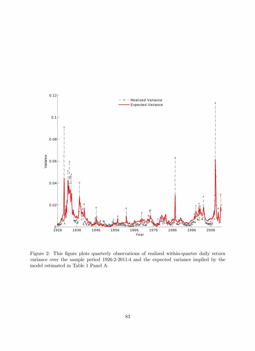
1926 1936 1946 1956 1966 1976 1986 1996 20060

0.02

0.04

0.06

0.08

0.1

0.12

Varia

nce

Year

Real ized VarianceExpected Variance

Figure 2: This figure plots quarterly observations of realized within-quarter daily returnvariance over the sample period 1926:2-2011:4 and the expected variance implied by themodel estimated in Table 1 Panel A.

83

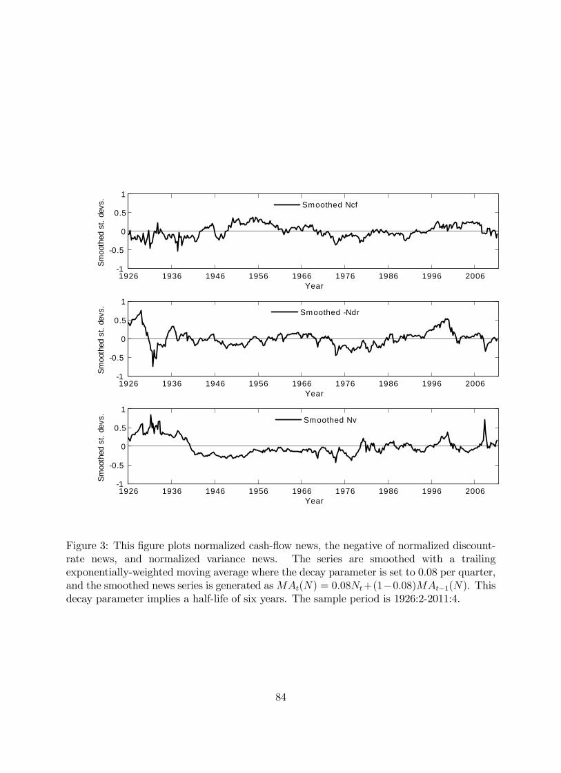
1926 1936 1946 1956 1966 1976 1986 1996 20061

0.5

0

0.5

1

Smoo

thed

st.

devs

.

Year

Smoothed Ncf

1926 1936 1946 1956 1966 1976 1986 1996 20061

0.5

0

0.5

1

Smoo

thed

st.

devs

.

Year

Smoothed Ndr

1926 1936 1946 1956 1966 1976 1986 1996 20061

0.5

0

0.5

1

Smoo

thed

st.

devs

.

Year

Smoothed Nv

Figure 3: This figure plots normalized cash-flow news, the negative of normalized discount-rate news, and normalized variance news. The series are smoothed with a trailingexponentially-weighted moving average where the decay parameter is set to 0.08 per quarter,and the smoothed news series is generated asMAt(N) = 0.08Nt+(1−0.08)MAt−1(N). Thisdecay parameter implies a half-life of six years. The sample period is 1926:2-2011:4.

84

1930 1940 1950 1960 1970 1980 1990 20004

2

0

2

4

6

Sta

ndar

d D

evia

tions

Y ear

10y r LHRVARlagged DEFlagged PE

1930 1940 1950 1960 1970 1980 1990 20000

0.02

0.04

0.06

0.08

0.1

10y

r LH

RV

AR

Y ear

10y r LHRVARForecasted Value

Figure 4: We measure long-horizon realized variance (LHRV AR) as the annualized dis-

counted sum of within-quarter daily return variance, LHRV ARh =4∗Σhj=1ρj−1RV ARt+j

Σhj=1ρj−1 . Each

panel of this figure plots quarterly observations of ten-year realized variance, LHRV AR40,over the sample period 1930:1-2001:1. In Panel A, in addition to LHRV AR40, we also plotlagged PE and DEF . In Panel B, in addition to LHRV AR40, we also plot the fitted valuefrom a regression forecasting LHRV AR40 with DEFO, defined as DEF orthogonalized todemeaned PE. Table 4 Panel B reports the WLS estimates of this forecasting regression.

85

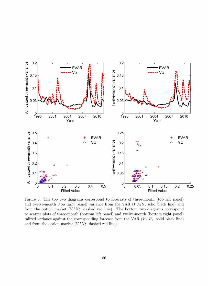
Figure 5: The top two diagrams correspond to forecasts of three-month (top left panel)and twelve-month (top right panel) variance from the VAR (V ARh, solid black line) andfrom the option market (V IX2

h, dashed red line). The bottom two diagrams correspondto scatter plots of three-month (bottom left panel) and twelve-month (bottom right panel)ralized variance against the corresponding forecast from the VAR (V ARh, solid black line)and from the option market (V IX2

h, dashed red line).

86

0 0.2 0.4 0.6 0.8

0.5

0

0.5

1

RVAR

ln re

al m

arke

t ret

urn

earlymodern

0.1 0 0.1 0.2 0.30.6

0.4

0.2

0

0.2

0.4

0.6

0.8

Nvln

real

mar

ket r

etur

n

earlymodern

3 4 5 6 71.5

2

2.5

3

3.5

4

DEFO

ln P

E

earlymodern

2 1 0 1 20.6

0.4

0.2

0

0.2

0.4

0.6

0.8

deltaDEFO

ln re

al m

arke

t ret

urn

earlymodern

Figure 6: The top left portion of the figure plots the market return against RV AR. The topright portion of the figure plots the market return against volatility news, NV . The bottomleft of the figure plots PE against DEFO (DEF orthogonalized to PE). The bottom rightof the figure plots market returns against the contemporaneous change in DEFO, our simpleproxy for news about long-horizon variance. In all four subplots, observations from the earlyperiod as denoted with blue triangles while observations from the modern period data aredenoted with red asterisks.

87

0 10 20 300

5

10

15

20

25

30

ICAPM with zerobeta rate0 10 20 30

0

5

10

15

20

25

30

ICAPM with riskfree rate

0 10 20 300

5

10

15

20

25

30

CAPM with zerobeta rate0 10 20 30

0

5

10

15

20

25

30

CAPM with riskfree rate

Figure 7: The four diagrams correspond to (clockwise from the top left) the CAPM witha constrained zero-beta rate, the CAPM with an unconstrained zero-beta rate, the three-factor ICAPMwith a free zero-beta rate, and the three-factor ICAPMwith the zero-beta rateconstrained to the risk-freee rate. The horizontal axes correspond to the predicted averageexcess returns and the vertical axes to the sample average realized excess returns for the 25ME- and BE/ME-sorted portfolios. The predicted values are from regressions presented inTable 7 for the sample period 1931:3-1963:2.

88

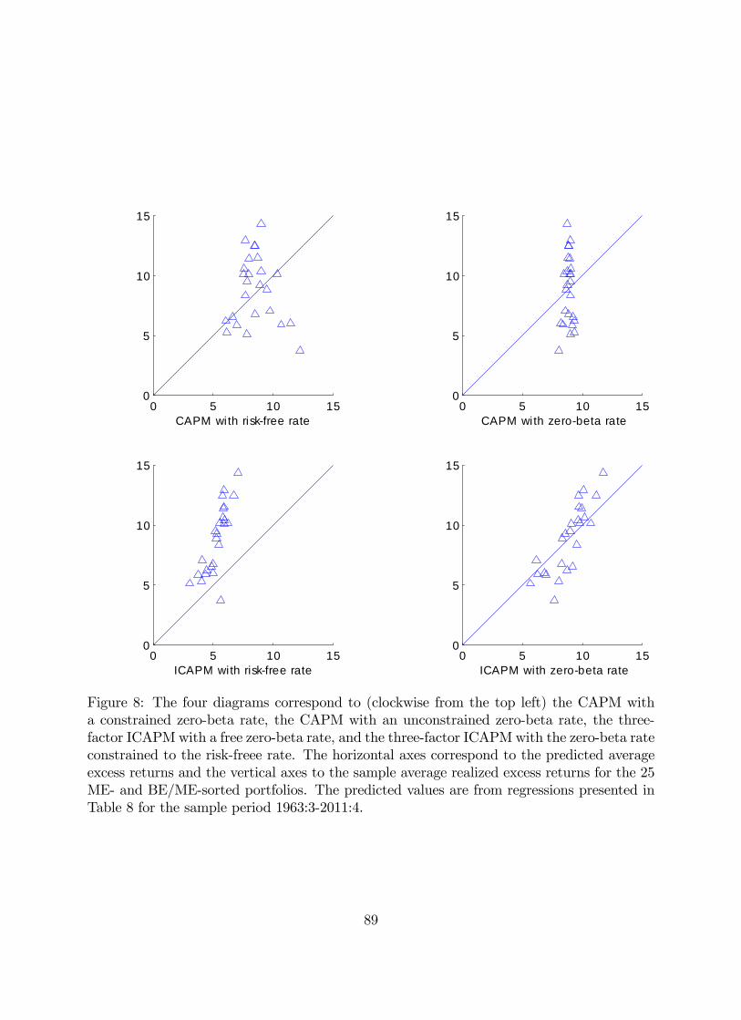
0 5 10 150

5

10

15

ICAPM with zerobeta rate0 5 10 15

0

5

10

15

ICAPM with riskfree rate

0 5 10 150

5

10

15

CAPM with zerobeta rate0 5 10 15

0

5

10

15

CAPM with riskfree rate

Figure 8: The four diagrams correspond to (clockwise from the top left) the CAPM witha constrained zero-beta rate, the CAPM with an unconstrained zero-beta rate, the three-factor ICAPMwith a free zero-beta rate, and the three-factor ICAPMwith the zero-beta rateconstrained to the risk-freee rate. The horizontal axes correspond to the predicted averageexcess returns and the vertical axes to the sample average realized excess returns for the 25ME- and BE/ME-sorted portfolios. The predicted values are from regressions presented inTable 8 for the sample period 1963:3-2011:4.

89

0

0

0

0.1

0.1

0.2

0.2

0.3

0.3

0.3

0.4

0.4

0.4

0.5

0.5

0.6

0.6

0.7

omeg

a

gamma

Riskfree rate, modern period

0 5 10 15 20 25 30 35 400

10

20

30

40

Crosssectional R 2

ICAPM

0

0.1

0.1

0.2

0.2

0.3

0.3

0.3

0.4

0.40.4

0.4

0.5

0.5

0.50.5

0.5

0.6

0.6

0.6

0.6

0.7

0.7

0.7

omeg

a

gamma

Zerobeta rate, modern period

0 5 10 15 20 25 30 35 400

10

20

30

40

Crosssectional R 2

ICAPM

Figure 9: The two contour plots show how the R2 of the cross-sectional regression explainingthe average returns on the 25 size- and book-to-market portfolios varies for different valuesof γ and ω for the risk-free rate (top panel) and zero-beta rate (bottom panel) three-betaICAPM model estimated in Table 8 for the sample period 1963:3-2011:4. The two plots alsoindicate the ICAPM relation between γ and ω described in equation (24).

90

1926 1946 1966 1986 20061

0.5

0

0.5

1

Smoo

thed

st.

devs

.

Year

CAPM

1926 1946 1966 1986 20061

0.5

0

0.5

1

Smoo

thed

st.

devs

.

Year

TwoBeta ICAPM

1926 1946 1966 1986 20061

0.5

0

0.5

1

Smoo

thed

st.

devs

.

Year

Threebeta ICAPM

Figure 10: This figure plots the time-series of the smoothed combined shock for the CAPM(NCF−NDR), the two-beta ICAPM (γNCF−NDR), and the three-beta ICAPM that includesstochastic volatility (γNCF−NDR− 1

2ωNV ) for the unconstrained zero-beta rate specifications

estimated in Table 8 for the modern subperiod. The shock is smoothed with a trailingexponentially-weighted moving average. The decay parameter is set to 0.08 per quarter, andthe smoothed news series is generated as MAt(SDF ) = 0.08SDFt + (1 − 0.08)MAt−1(N).This decay parameter implies a half-life of six years. The sample period is 1926:2-2011:4.

91

An Intertemporal CAPM with Stochastic Volatility -...

Documents

Transcript of An Intertemporal CAPM with Stochastic Volatility -...