
AN INTELLIGENT HUMAN-TRACKING ROBOT BASED-ON …
134
AN INTELLIGENT HUMAN-TRACKING ROBOT BASED-ON KINECT SENSOR A Thesis by JINFA CHEN Submitted to the Office of Graduate and Professional Studies of Texas A&M University in partial fulfillment of the requirements for the degree of MASTER OF SCIENCE Chair of Committee, Won-jong Kim Committee Members, Sivakumar Rathinam Zhizhang Xie Head of Department, Andreas A. Polycarpou December 2015 Major Subject: Mechanical Engineering Copyright 2015 Jinfa Chen
Transcript of AN INTELLIGENT HUMAN-TRACKING ROBOT BASED-ON …

AN INTELLIGENT HUMAN-TRACKING ROBOT BASED-ON KINECT SENSOR
A Thesis
by
JINFA CHEN
Submitted to the Office of Graduate and Professional Studies of
Texas A&M University
in partial fulfillment of the requirements for the degree of
MASTER OF SCIENCE
Chair of Committee, Won-jong Kim
Committee Members, Sivakumar Rathinam
Zhizhang Xie
Head of Department, Andreas A. Polycarpou
December 2015
Major Subject: Mechanical Engineering
Copyright 2015 Jinfa Chen

ii
ABSTRACT
This thesis provides an indoor human-tracking robot, which is also able to
control other electrical devices for the user. The overall experimental setup consists of a
skid-steered mobile robot, Kinect sensor, laptop, wide-angle camera and two lamps. The
Kinect sensor is mounted on the mobile robot to collect position and skeleton data of the
user in real time and sends it to the laptop. The laptop processes these data and then
sends commands to the robot and the lamps. The wide-angle camera is mounted on the
ceiling to verify the tracking performance of the Kinect sensor. A C++ program runs the
camera, and a java program is used to process the data from the C++ program and the
Kinect sensor and then sends the commands to the robot and the lamps. The human-
tracking capability is realized by two decoupled feedback controllers for linear and
rotational motions. Experimental results show that although there are small delays (0.5 s
for linear motion and 1.5 s for rotational motion) and steady-state errors (0.1 m for linear
motion and 1.5° for rotational motion), tests show that they are acceptable since the
delays and errors do not cause the tracking distance or angle out of the desirable range
(±0.05m and ± 10° of the reference input) and the tracking algorithm is robust. There are
four gestures designed for the user to control the robot, two switch-mode gestures, lamp
crate gesture, and lamp-selection and color change gesture. Success rates of gestures
recognition are more than 90% within the detectable range of the Kinect sensor.

iii
ACKNOWLEDGEMENTS
First of all, I would like to thank my advisor, Dr. Won-jong Kim, for his
guidance and help throughout my research. Dr. Kim has always been patient and
encouraging with great advice. I would also like to thank Enrique Zarate, a former
undergraduate student, for the construction of the mobile robot used in this research.
I would like to thank my committee members, Drs. Rathinam and Xie for serving
on my thesis committee and for being patient with and understanding me.
Thanks also go to my friends, lab mates and the department faculty and staff for
making my time at Texas A&M University be a great experience.
Finally, thanks to my mother and father for their encouragement and to my
girlfriend, Tianmei Zhang, for her patience and love.
iv
TABLE OF CONTENTS
Page
ABSTRACT .......................................................................................................................ii
ACKNOWLEDGEMENTS ............................................................................................. iii
TABLE OF CONTENTS .................................................................................................. iv
LIST OF FIGURES ..........................................................................................................vii
LIST OF TABLES ............................................................................................................ xi
CHAPTER I INTRODUCTION AND LITERATURE REVIEW ................................... 1
1.1 Design objectives ................................................................................................. 1 1.2 Human tracking .................................................................................................... 1
1.3 Gesture recognition .............................................................................................. 2 1.4 Applications ......................................................................................................... 3
1.4.1 Home entertainment ................................................................................... 3 1.4.2 Automotive ................................................................................................. 4 1.4.3 Television ................................................................................................... 5
1.4.4 Mobile devices ........................................................................................... 6 1.5 Thesis overview ................................................................................................... 6
1.6 Thesis contributions ............................................................................................. 7
CHAPTER II DESIGN AND SYSTEM ARCHITECTURE ............................................ 9
2.1 Hardware components ......................................................................................... 9 2.1.1 Skid-Steered mobile robot .......................................................................... 9
2.1.2 Kinect sensor ............................................................................................ 10 2.1.3 Assemble of the Kinect sensor ................................................................. 12 2.1.4 A wide-angle camera ................................................................................ 13 2.1.5 Devices to be controlled ........................................................................... 14
2.2 Software components ......................................................................................... 14
2.2.1 Processing ................................................................................................. 14 2.2.2 OpenNI ..................................................................................................... 15 2.2.3 Arduino IDE ............................................................................................. 15
2.2.4 MATLAB ................................................................................................. 16 2.2.5 OpenCV .................................................................................................... 16 2.2.6 Visual Studio 2010 ................................................................................... 17

v
2.3 Connection ......................................................................................................... 17
CHAPTER III CONTROL SYSTEM DESIGN .............................................................. 21
3.1 Mathematical modeling ..................................................................................... 21 3.1.1 Model description ..................................................................................... 21
3.1.2 Definitions of parameters ......................................................................... 21 3.1.3 Kinematics ................................................................................................ 24 3.1.4 Dynamic modeling ................................................................................... 27
3.2 System analysis .................................................................................................. 31 3.2.1 Stability .................................................................................................... 31 3.2.2 Open-loop dynamics ................................................................................ 33
3.3 Classical control design ..................................................................................... 37
3.3.1 PID controller ........................................................................................... 37 3.3.2 Lead-lag controller ................................................................................... 40
3.4 Simulation .......................................................................................................... 49 3.4.1 PID controller ........................................................................................... 51
3.4.2 Lead-lag controller ................................................................................... 52 3.5 Technical discussion and evaluation .................................................................. 54
CHAPTER IV HUMAN-ROBOT INTERACTION DESIGN ........................................ 55
4.1 Human tracking .................................................................................................. 56
4.1.1 Human tracking with the Kinect sensor ................................................... 56 4.1.2 Human tracking with the wide-angle camera ........................................... 60
4.1.3 The whole process of tracking ................................................................. 66 4.2 Gesture control ................................................................................................... 69
4.2.1 Skeleton tracking ...................................................................................... 70
4.2.2 Gesture definition ..................................................................................... 71 4.2.3 Gesture control ......................................................................................... 76
CHAPTER V EXPERIMENTAL RESULTS .................................................................. 77
5.1 Human-tracking evaluation ................................................................................ 78 5.1.1 Experimental design ................................................................................. 78 5.1.2 Results ...................................................................................................... 82
5.2 Gesture recognition evaluation .......................................................................... 93 5.2.1 Experimental design ................................................................................. 94 5.2.2 Results ...................................................................................................... 94
CHAPTER VI CONCLUSIONS AND FUTURE WORK .............................................. 96
6.1 Conclusions ........................................................................................................ 96 6.2 Future work ........................................................................................................ 97

vi
REFERENCES ................................................................................................................. 99
APPENDIX .................................................................................................................... 102
Processing Code ...................................................................................................... 102 Matlab Code ............................................................................................................ 114
C ++ Code .............................................................................................................. 117

vii
LIST OF FIGURES
Page
Figure 1-1 Skeleton image shown on a computer while a human is being tracked ........... 3
Figure 1-2 Toyota’s fully electric car equipped with Kinect sensors [5] ........................... 4
Figure 1-3 Mercedes-Benz gesture-control concept [6] ..................................................... 5
Figure 2-1 The skid-steered mobile robot used in the research ....................................... 11
Figure 2-2 The Kinect sensor ........................................................................................... 11
Figure 2-3 The structure to carry the Kinect sensor ......................................................... 12
Figure 2-4 the wide-angle camera (ELP-USB500W02M-L36) [19] ............................... 14
Figure 2-5 Communication among various devices ......................................................... 18
Figure 2-6 Cooperation among software components ..................................................... 19
Figure 3-1 Dimension definitions of the vehicle .............................................................. 22
Figure 3-2 The electric circuit of the armature................................................................. 23
Figure 3-3 Schematic diagram for circular motion of the mobile robot .......................... 28
Figure 3-4 The block diagram of the system .................................................................... 32
Figure 3-5 The Root locus of the system for linear motion only ..................................... 33
Figure 3-6 The Root locus of the system for rotational motion only ............................... 34
Figure 3-7 Step response with same torque input ............................................................ 35
Figure 3-8 Step response with different torque input ....................................................... 36
Figure 3-9 Step response with different proportional torque input .................................. 37
Figure 3-10 The block diagram of the system with controller ......................................... 38
Figure 3-11 Step response of the closed-loop system (linear motion) ............................. 39

viii
Figure 3-12 Step response of the closed-loop system (rotation) ...................................... 40
Figure 3-13 Bode plot of the plant with control gain (linear motion) .............................. 42
Figure 3-14 Bode plot for lag compensation .................................................................... 43
Figure 3-15 Step response of the system with lag compensation .................................... 44
Figure 3-16 Bode plot for the lead compensation ............................................................ 46
Figure 3-17 Step response of the system with the lead compensation ............................. 47
Figure 3-18 Bode plot of the plant with the lead compensation (linear motion) ............. 47
Figure 3-19 Bode plot for the lead-lag compensation ...................................................... 49
Figure 3-20 Step response of the system with lead-lag compensation ............................ 49
Figure 3-21 The system simulated in Simulink ............................................................... 50
Figure 3-22 Simulation result of PID controller for linear motion .................................. 51
Figure 3-23 Simulation result of PID controller for rotational motion ............................ 52
Figure 3-24 Simulation result of the lag compensation for linear motion ....................... 53
Figure 3-25 Simulation result of the lead compensation for linear motion ..................... 53
Figure 3-26 Simulation result of the lead-lag compensation for linear motion ............... 54
Figure 4-1 Flowchart of the whole interaction system ..................................................... 55
Figure 4-2 Reference coordinates of the Kinect sensor ................................................... 57
Figure 4-3 The top view of the user in the Kinect’s coordinates ..................................... 58
Figure 4-4 The front view of the user in the Kinect’s coordinates................................... 59
Figure 4-5 Graphical user interface for tracking mode .................................................... 59
Figure 4-6 A schematic of a camera view ........................................................................ 61
Figure 4-7 Tracking by the camera .................................................................................. 62

ix
Figure 4-8 A schematic of camera capturing in front view .............................................. 63
Figure 4-9 A schematic of camera capturing in left view ................................................ 65
Figure 4-10 A schematic of camera capturing in top view .............................................. 67
Figure 4-11 Flowchart of the human-tracking system ..................................................... 68
Figure 4-12 GUI for gesture controlling mode ................................................................ 70
Figure 4-13 The Skeleton that the Kinect sensor tracks ................................................... 71
Figure 4-14 Scheme of the gesture to switch to gesture controlling mode ...................... 73
Figure 4-15 Scheme of the gesture to switch to tracking mode ....................................... 73
Figure 4-16 Scheme of the lamp creating gesture ............................................................ 74
Figure 4-17 Scheme of the lamp selecting and color changing gestures ......................... 75
Figure 4-18 Flowchart of the gesture-control system ...................................................... 76
Figure 5-1 Experimental platform .................................................................................... 78
Figure 5-2 Configuration of the linear motion experiment .............................................. 79
Figure 5-3 Configuration of the rotation experiment ....................................................... 81
Figure 5-4 Experimental result of the lead-lag controller (1 m) ...................................... 83
Figure 5-5 Experimental result of the lead-lag controller (0.5 m) ................................... 85
Figure 5-6 Experimental result of the lead-lag controller (1m) ....................................... 85
Figure 5-7 Experimental result of the lead-lag controller (0.5m) .................................... 86
Figure 5-8 Experimental result of the PID controller for rotation (10°) .......................... 87
Figure 5-9 Experimental result of the PID controller for rotation (15°) .......................... 88
Figure 5-10 Experimental result of the PID controller for rotation (20°) ........................ 89
Figure 5-11 Experimental result of the combined performance with the initial distance of
1 m and initial angle of 10° (distance response) ....................................................... 90

x
Figure 5-12 Experimental result of the combined performance with the initial distance of
1 m and the initial angle of 10° (angle response) ...................................................... 91
Figure 5-13 Experimental result of combination performance with the initial distance of
1 m and the initial angle of 15° (distance response) ................................................. 92
Figure 5-14 Experimental result of the combined performance with the initial distance of
1 m and the initial angle of 15° (angle response) ...................................................... 92
Figure 5-15 Trajectories of the robot and the user ........................................................... 93

xi
LIST OF TABLES
Page
Table 3.1 Summarizes the key parameters of the robot ................................................... 25
Table 3.2 Define the variables of the robot to be used in the rest of thesis ..................... 26
Table 5.1 Success rate of the gesture recognition ............................................................ 95

1
CHAPTER I
INTRODUCTION AND LITERATURE REVIEW
1. Chapter1
Electronic devices are ubiquitous these days. With the development of computer
vision technology and depth cameras, the ways people interact with the electrical devices
are being improved. Low-cost depth cameras have been researched for years with newly
available techniques, and the development of software and algorithms for them enhances
their functions. The release of low-cost depth cameras allows more and more people to
enjoy the benefit of this technology.
1.1 Design objectives
The objective of this thesis is to develop a human-tracking intelligent robot to
improve the way that humans interact with electronic devices. This robot is designed
mainly for the household and is capable of doing the following:
1. Tracking the designated person quickly and smoothly on a flat wooden floor
or carpet, maintaining a safe distance to that person
2. Recognizing specific predetermined postures by the person being tracked
quickly and accurately
3. Controlling other electronic devices wirelessly based on the motion-
commands by the person being tracked.
1.2 Human tracking
There are several sensors that can be used for human tracking. Ultrasonic sensors

2
transmit and receive ultrasonic waves and determine the distance to an object by
calculating the time interval between sending the signal and receiving the echo. They are
used to track a human and avoid obstacles by developing an ultrasonic-sensor array [1].
However, ultrasonic sensors cannot distinguish humans from objects. RGB cameras,
which can deliver the three basic color components (red, green, and blue), are frequently
used some image processing software for object detection and tracking. For example,
OpenCV, Matlab, and Point Cloud Library (PCL) can be used for image processing.
However, 3D motion sensors (or depth sensors) are very likely to supersede other
sensors in human tracking due to their reliability and depth sensing ability.
A 3D motion sensor is a device that can capture motions in 3D [2], [3]. There are
two popular commercial 3D motion sensors, Kinect from Microsoft and Xtion PRO Live
from Asus. The Kinect sensor has high resolution (1–75mm) [4] and is more adaptable
than the Xtion PRO Live. Human-tracking is easy to realize with 3D motion sensors
because they usually come with a software development kit (SDK) that processes color,
depth, and skeleton data. With these data, it is convenient to create human-tracking
applications.
1.3 Gesture recognition
Gesture recognition is an application based on skeleton tracking. Skeleton
tracking is a key function of the 3D motion sensor that allows the sensor to recognize
humans. As shown in Figure 1-1, a human is being tracked by a Kinect sensor, and his
skeleton image with a coordinate in each joint is shown on the computer monitor in real
time. By locating these joints, the distance between of two joints and the angle of three

3
joints can be calculated. While a specific gesture has a certain distance between two
joints and angle ranges of three joints, gesture recognition can be realized by setting the
combination of angle ranges and distance between these joints and defining them. For
the Kinect sensor, up to six people can be recognized and up to two people can be
tracked in detail within the detectable field of the sensor.
Figure 1-1 Skeleton image shown on a computer while a human is being tracked
1.4 Applications
Motion-control techniques are applied in a variety of areas listed below.
1.4.1 Home entertainment
The Xbox 360 Kinect Sensor may not be the first application of motion control

4
but must be the most popular application. The Xbox 360 Kinect Sensor is a motion
sensing input device by Microsoft for the Xbox 360 video game console. Based on a
Kinect sensor for the Xbox 360 console, it enables users to control and interact with the
console without touching any game controller, only through a natural user interface
using gestures and spoken commands.
1.4.2 Automotive
Toyota has unveiled the ‘Smart Insect’ concept at CEATEC technology show
2012 in Japan. The fully electric car, as shown in Figure 1-2, is decked out with a Kinect
sensor by Microsoft. The on-board motion sensors allow the car to recognize its owner
based on face and body shapes and predict the owner's behavior by analyzing movement.
For example, it can detect the approaching of the owner and determine when to open the
door.
Figure 1-2 Toyota’s fully electric car equipped with Kinect sensors [5]

5
The front and rear displays are set to show a welcome message when the owner
approaches the car. The car is equipped with a speaker on the hood of the car and
dashboard-mounted microphones on the front and back, so voice recognition is also
included for opening the car door and other functions [5].
Mercedes’ Dynamic & Intuitive Control Experience (DICE) built a concept cabin
by installing a series of proximity sensors to detect arm and hand movements. With
those sensors users can control everything from music, navigation, and social
functionality to a heads-up display that comprises the entire windshield [6], as shown in
Figure 1-3.
Figure 1-3 Mercedes-Benz gesture-control concept [6]
1.4.3 Television
TCL Multimedia (TCL), one of China’s leading TV and consumer electronics

6
brands, begins to use Hillcrest’s Freespace motion software for its Smart TVs. The
Freespace gesture recognition engine enables motion, gesture, and cursor control for the
user to navigate and interact with the smart TV content. It includes the TV menus, Web
browser, games, and a wide variety of applications [7].
1.4.4 Mobile devices
Depth sensors are also applied in mobile devices. Earlier this year, Google
introduced its Project Tango smartphone, a mobile device equipped with a depth sensor,
a motion tracking camera, and two vision processors that enable the phone track its
position in space and create 3D maps in real time [8]. The device is not only a phone but
also a good sensor for robot since it is the base capability for most of the robots to
navigate and locate themselves in the real world.
1.5 Thesis overview
The thesis consists of six chapters: Introductions, Design and System
Architecture, Control System Design, Human-Robot Interaction Design, Simulation and
Experimental Results, Conclusions and Future work.
The thesis begins with the first chapter, giving an introduction to human-tracking
mobile robot and applications. This introduction also covers thesis overview and
significance of thesis contributions.
In the second chapter, the hardware and software components of the system are
described. This chapter presents the function of each hardware and software components
and clarifies how they work with each other.

7
The third chapter details the control system design. In this chapter, a
mathematical model is derived and analyzed. Based on these analyses, two proportional-
integral-derivative (PID) controllers and a lead-lag compensation are designed. Finally,
all these controllers are simulated and evaluated.
The fourth chapter introduces the design of human-robot interaction. This chapter
mainly describes the functions expected from the mobile robot and how they are coded.
The fifth chapter describes the experiments designed for both human tracking
and gesture recognition. Along with this, the experimental results are also given and
discussed.
The final chapter entails the conclusions of the thesis and provides an insight into
the experiments with suggestions for improvements.
1.6 Thesis contributions
A structure was built on the mobile robot by Enrique Zarate, a former
undergraduate student in our lab, to carry the Kinect sensor. A mathematical model was
developed by identifying necessary parameters. The robot’s motions were decoupled
into linear motion and rotational motion. Based on this model, a proportional-integral-
derivative (PID) controller was designed for the rotational motion control, and a PID,
lead, lag, and a lead-lag controllers were designed for the linear motion control. A wide-
angle camera was installed on the ceiling of the lab. A C++ program was written to
process the video stream of the camera and track the position of the user and the robot.
Two lamps controlled by Arduino boards were developed. Java programs were written
for the Arduino boards. The Kinect sensor was used to obtain 3D position data and

8
skeleton data of the user being tracked. A Java program was written to process these data
from the Kinect sensor and the camera and then send commands to the Arduino board.
The controllers were implemented in the main Java program to process these position
data. Gestures to command the robot were designed and included in the main Java
program. Experiments were conducted to evaluate the performance of the tracking
ability and the gesture recognition of the robot.

9
CHAPTER II
DESIGN AND SYSTEM ARCHITECTURE
2.
In this chapter, the hardware and software of the robot are introduced, and then
the functions of these components and how they work with each other are clarified.
2.1 Hardware components
2.1.1 Skid-Steered mobile robot
Skid-steered mobile robots are widely used due to their robust mechanical
structure and high maneuverability. Although much research was conducted on dynamic
modeling and tracking control of differential-driven mobile robots, not as much research
has been done on skid-steered mobile robots. A kinematic model for an ideal
differential-driven wheeled robot cannot be categorized as a skid-steered robot because
the effects of skidding and slipping of robot wheels are minimal. Recently, many
researchers developed mathematical models of skid-steered mobile robots, considering
the effect between wheels and the ground. Yi et al. [9] proposed a pseudo-static friction
model. Although a skid-steered mobile robot usually assumes all wheels on the same
side share the same speed, a dynamic model with different angular velocities of four
wheels was developed [10]. In [11], the kinematic model included the effects of slippage
without dynamics computations in the loop. In this research, a model proposed in [12]
was simplified and adopted since the model in that paper is described in terms of the

10
angular velocity of the wheels, which is beneficial and easy for control.
Based on the aforementioned models, researchers also developed control
algorithms. In [13], a tuning fuzzy vector field orientation (FVFO) feedback control
method was proposed for a skid-steered mobile robot using flexible fuzzy logic control
(FLC). In [14], a robust backstepping tracking control was proposed based on a
Lyapunov redesign for a skid-steered mobile robot.
Most of the skid-steered mobile robots have four wheels [9], [10] and [12].
However, some of them have two wheels [14], and six wheels [15]. The majority of
skid-steered mobile robots are wheeled [9], [10], [12], [14]–[16], but some are tracked
[13], [17] to handle the tough terrain. In this research, a four-wheeled skid-steered
mobile robot is used.
Figure 2-1 is the skid-steered mobile robot that is used in the research. It was
built by Enrique Zarate, a former undergraduate student in our lab. This mobile robot
was controlled by an Arduino board and was actuated by four motors. Two motors on
each side are in parallel connection, which means wheels on the same side rotate in the
same direction and have the same angular velocity. On a flat surface, the vehicle has two
degrees of freedom (translation and rotation).
2.1.2 Kinect sensor
The Kinect sensor, seen Figure 2-2, is a motion sensing device by Microsoft. It
was originally designed for video gaming. However, developers also created
applications for human-robot interaction [18].

11
Figure 2-1 The skid-steered mobile robot used in the research
Figure 2-2 The Kinect sensor
Microsoft released a version of the Kinect sensor especially for windows. The
sensor contains two cameras (one RGB camera and one IR camera), a microphone array,

12
and a tilt motor as well as a software package that processes color, depth, and skeleton
data. Thus, users are able to create interactive applications that based on the recognition
of natural movements, gestures, and voice commands.
2.1.3 Assemble of the Kinect sensor
To mount the Kinect sensor on the robot, the top of the robot needs a structure
that can keep the Kinect sensor tight all the time. Also, this structure should be able to be
installed on the robot. There is nothing better than using a Kinect TV mount to attach a
Kinect sensor without dissembling it because there is nothing but two holes designed to
fit with that mount on the bottom of a Kinect sensor. However, the Kinect TV mount is
not designed to mount the Kinect sensor on the robot. Therefore, the mount was
modified to the one as shown in Figure 2-3.
Figure 2-3 The structure to carry the Kinect sensor

13
The best height of the Kinect sensor for human-tracking is about 0.5–1.5 m, but
the robot is just of 0.15 meter’s height. On the one hand, the tilt angle of the Kinect
sensor can be adjusted for sensing. However, the performance will become worse as the
tilt angle becomes large. On the other hand, a higher structure can be built to allow a
smaller tilt angle. However, the higher the Kinect sensor is mounted, the more unstable
the robot will become. With the best-fit sensing angle found experimentally, a structure
was built on top of the mobile robot to carry the Kinect sensor, as shown in Figure 2-3.
2.1.4 A wide-angle camera
The wide-angle camera used in the research, as shown in Figure 2-4, is a USB
camera from ELP, a manufacturer of surveillance system. The camera is come with a 5-
megapixel (MP) complementary metal–oxide–semiconductor (CMOS) sensor and a 3.6
mm lens. This configuration is ideal for the research because: 1) although 5 MP is a very
entry-level configuration for a camera, it is able to stream image clear enough for the
research. Higher resolution than 5 MP would be a waste; 2) the camera is supposed to be
mounted on the ceiling of the lab (3-m height), so theoretically 4.6 (horizontal) × 3.5
(vertical) m2 of floor area can be captured by the 3.6 mm lens. In case larger space is
need for experiments, a 2.1mm lens can also be purchased.
Another important characteristic of the camera is its 30 frames per second (FPS)
frame rate. Since the camera is to be mounted on the ceiling, a long USB extension cable
is need to connect the camera to the computer. Tests show that the long cable will not
slow down the frame rate under 30 FPS. The camera’s object detectable distance is
between 5 cm to 100 m, which is good enough for the research.

14
Figure 2-4 the wide-angle camera (ELP-USB500W02M-L36) [19]
2.1.5 Devices to be controlled
Any electrical device installed with a receiver can be controlled by the robot. In
the research, two lamps are built to indicate the remote control ability of the robot. The
lamp is made up with an Arduino board, a XBee receiver, two LEDs (one RGB LED and
one white LED), resistors and wires. The white LED is used to indicate whether the
power of the lamp is on or off. It is on to inform a user that it is waiting for the robot’s
commands. The RGB LED adopted in the research has full colors. It is used to indicate
the color of the lamp.
2.2 Software components
2.2.1 Processing
Processing is an open-source programming language and integrated development

15
environment (IDE) built on the Java language but using a simplified syntax and graphics
programming model, which is the reason it was adopted to compile the main program. In
this research, a program is need to process data from various sources (the Kinect and the
camera), and communicate with Arduino boards (robot and lamps). It is easy to
communicate Processing with Arduino, which is also java based, through serial port.
Besides, there are libraries for the Processing to process data from the Kinect and
camera. Therefore, Processing is the best choice to write the main program in the
research.
2.2.2 OpenNI
OpenNI (Open Natural Interaction), an industry-led, non-profit organization, was
created by PrimeSense, an company which developed the technology behind the
Kinect’s 3D imaging and worked with Microsoft to develop the Kinect device [20]. In
this research, OpenNI will be used as middleware to access the Kinect data streams and
the skeleton/hand tracking capability and as a library in Processing to obtain data from
the Kinect sensor.
2.2.3 Arduino IDE
The Arduino IDE is a cross-platform application written in Java, and derives
from the IDE for the Processing programming language and the Wiring projects [21]. In
this research, it was used to compile program for Arduino board inside the robot and the
lamps. Arduino IDE has a useful tool for debugging and monitoring serial ports, called
Serial Monitor. The Serial Monitor is a useful tool that acts as a separate terminal that

16
communicates by receiving and sending Serial Data. That makes the Arduino IDE
effective.
2.2.4 MATLAB
MATLAB is a high-level language, providing interactive environments for
numerical computation, visualization, and programming, that was developed by
MathWorks. MATLAB allows matrix manipulations, plotting of functions and data,
implementation of algorithms, creation of user interfaces, and interfacing with programs
written in other languages, for example, C++ and Java. MATLAB, in this research,
serves as a tool to tune the controllers designed for human-tracking, simulate motion
response of the robot, and analyze the experimental results.
2.2.5 OpenCV
Open Source Computer Vision (OpenCV) is a library of programming functions
mainly for real-time image processing. It can be used in, for example, C, C++, and Java
interfaces and supports operating system such as Windows, Linux, and Mac OS. In the
research, the OpenCV library was included in the C++ program to process the video
stream from the wide-angle camera. The OpenCV is mainly used for camera calibration
and color tracking. Pinhole cameras have come to our daily life for a long time. They are
compact and cheap. However, this cheapness comes with its price. Cheap cameras come
with significant distortion, especially in a wide-angle camera. Luckily, this problem can
be fix by calibration and some remapping. Furthermore, calibration relates the image
units (pixels) and the length units in real world (for example meters). That is the reason

17
OpenCV is adopted in the research.
2.2.6 Visual Studio 2010
Microsoft Visual Studio is an integrated development environment (IDE) from
Microsoft. It is a popular IDE for the C++ programing language on the Microsoft
Windows operating system. The reason Visual Studio is chosen for the research is that
OpenCV is adopted as a helpful library to process image from the wide-angle camera.
Visual Studio is recommended to build applications with OpenCV on the Microsoft
Windows operating system.
2.3 Connection
The overall experimental system consists of three devices, as shown in Figure
2-5, a mobile robot, wide-angle camera, and digitally controlled lamp. The
communication between the mobile robot and the lamp is developed by a pair of XBee
radio modules. For the mobile robot, the XBee modules, Kinect sensor, Arduino board
and wide-angle camera are connected to the laptop through four USB data cables. For
the digital lamp, the other XBee module is connected to the Arduino board.
Figure 2-6 presents a diagram illustrating how the software components work
together. The camera is operated by a C++ program running with Visual Studio. This
program tracks a user and the mobile robot (to track specific colors) and sends
translational and angular data to the Processing program. As the C++ program runs, it
setups for the connection with the Processing program, but it does not start tracking until
the Processing program is ready to receive data. When the Processing program runs, it

18
makes a connection to the C++ Program. Once the connection is established
successfully, the camera start working and the whole system begins operating.
Arduino UNO
The Kinect Sensor
XBee module
XBee module
Arduino Uno
Wir
eles
s
USB
USB
USB
USB
Depth Sensing
The Mobile Robot
Devices To be controlled(e.g. Lamp)
CC
olo
rTr
acki
ngC
amer
a
Figure 2-5 Communication among various devices
There are two mode of the system, human-tracking mode and motion-control
mode. For the human-tracking mode, the Kinect sensor keeps detecting and sends depth
data to the laptop through a USB data cable. Then the Processing program, running in

19
the laptop, keeps receiving depth data by the OpenNI, and translational and angular data
by a socket, processes these data using the controller designed in Matlab, and sends
command data to the Arduino board on the robot through a serial port. The command
data are information about the velocities of the wheels on difference sides. The Arduino
board generates pulse width modulation (PWM) signal of appropriate duty cycle to
different motors based on the command data. Then the motors on the left side and the
right sides generate appropriate torques so that the robot can track the designated person.
MATLAB
The Kinect Sensor
Dep
th
Sen
sin
g
The Mobile Robot
Arduino IDE
OpenNI
Processing
Laptop
Controller
Visual Studio
OpenCV
Position Data
ColorTracking
Figure 2-6 Cooperation among software components

20
For the motion-control mode, the Kinect sensor keeps detecting and sends
positional data of joints of the person being tracked to the laptop. The Processing
program processing these data and sends PWM signals to the Arduino boards of the
lamps through the Xbee modules. Then the Arduino boards process these signals to
control LEDs in the lamps.

21
CHAPTER III
CONTROL SYSTEM DESIGN
3.
3.1 Mathematical modeling
In this section, critical parameters are measured and calculated, and the kinematic
and dynamic model of the mobile robot are developed.
3.1.1 Model description
The mobile robot used in this research is a skid-steered mobile robot. A skid-
steered mobile robot is a vehicle that steers by controlling the relative velocities of the
wheels or tracks on the left and right sides. Also, all the wheels or tracks always point to
the longitudinal axis of the vehicle. So, there is always slippage while a skid-steered
vehicle turns. There has been so much research on this type of mobile robot. After some
study, the model in [12] was adopted and revised.
3.1.2 Definitions of parameters
The robot is not of a regular shape, so it is not easy to calculate its moment of
inertia. To calculate the moment of inertia of the robot, the shape of it is simplified to
two solid cuboids representing the Kinect sensor and the vehicle, respectively. The solid
cuboid representing the Kinect sensor is of the mass 𝑀𝑘, width 𝑤𝑘, depth 𝑑𝑘, and height
ℎ𝑘, as shown in Figure 3-1.

22
Vehicle
Z
Kinect
Figure 3-1 Dimension definitions of the vehicle
𝑙𝑘 denotes the distance between the center of mass of the cuboid and the rotation
axis, and 𝑑𝑘𝑣 denotes the distance between the Kinect sensor and the vehicle body.
Since the Kinect sensor does not rotate about an axis through the body’s center of mass.
According to the parallel axis theorem, the moment of inertia of the Kinect sensor should
be:
𝑤𝑣
𝑤𝑘
𝑑𝑣
𝑑𝑘
ℎ𝑣
ℎ𝑘 𝑙𝑘
𝑑𝑘𝑣

23
𝐼𝑘 =
1
12𝑀𝑘(𝑤𝑘
2 + 𝑑𝑘2) + 𝑀𝑘𝑙𝑘
2 (3.1)
The solid cuboid representing the vehicle is of the mass 𝑀𝑣, width 𝑤𝑣, depth 𝑑𝑣,
and height ℎ𝑣. In this case, the moment of inertia of the vehicle is:
𝐼𝑣 =
1
12𝑀𝑣(𝑤𝑣
2 + 𝑑𝑣2) (3.2)
Therefore, the total moment of inertia of the robot is:
𝐼 = 𝐼𝑘 + 𝐼𝑣 (3.3)
A schematic diagram of a DC motor system is shown in Figure 3-2. In a
permanent-magnet DC motor, the developed torque is proportional to the armature
current 𝑖𝑚 with a torque constant 𝐾𝑡 as shown in the relation below.
𝑇𝑚 = 𝐾𝑡𝑖𝑚 (3.4)
V
R L
e
+
-Armature Rotor
Figure 3-2 The electric circuit of the armature
𝑻𝒎
𝒊𝒎

24
The datasheet of the motor does not list the torque constant of the DC motor.
Instead, it gives the torque 𝑇𝑎 = 0.012 kg-m at 3 V. Therefore, the current through each
motor of the vehicle at 3 V equals to the armature voltage divided by the armature
resistance.
𝐼𝑎 =
𝑉𝑎
𝑅𝑚= 1.36 A (3.5)
So the torque constant can be calculated by dividing torque by the current.
𝐾𝑡 =
𝑇𝑎
𝐼𝑎=
0.012 × 9.81 N ⋅ m
1.36 A= 0.0865 N‐m ∕ A (3.6)
In the Processing IDE, the range of the motor’s velocity 𝑝𝑣 is 0-255, assuming
that it is proportional to the motor’s angular velocity. Then
𝑖𝑚 = 𝑘𝑖 ⋅ 𝑝𝑣 (3.7)
𝑘𝑖 =1.36
255= 0.0053 A
𝛼 is a terrain-dependent that related to rolling resistance 𝜇𝑟. Experiments show
that the large the rolling resistance, the large the value of 𝛼 [12]. Referring to [12], 𝛼
was set to 1.5 for a lab surface. Both the frame rate of the Kinect sensor and the camera
are denoted by 𝑇𝑆. Table 3.1 lists all the important parameters of the robot.
3.1.3 Kinematics
In this section, the kinematics model of the robot is developed. Table 3.2 gives
all the variables that used in the mathematical modeling of the robot.

25
Table 3.1 Summarizes the key parameters of the robot
Mass of the vehicle 𝑀𝑣 = 1.0741 kg
Mass of the Kinect sensor 𝑀𝑘 = 0.4646 kg
Vehicle width 𝑤𝑣 = 0.172 m
Vehicle length 𝑑𝑣 = 0.199 m
Kinect width 𝑤𝑘 = 0.254 m
Kinect depth 𝑑𝑘=0.064 m
Mass of center of Kinect to the rotate axis 𝑙𝑘 = 0.023 m
Moment inertia of the robot 𝐼 = 0.0091 kg‐m2
Motor armature resistor 𝑅𝑚 = 2.2 Ω
Motor voltage 𝑉𝑎 = 3 V
Motor torque at 3 V 𝑇𝑎 = 0.012 kg‐m
Motor current at 3 V 𝐼𝑎 = 1.36 A
Gear ratio 𝐺𝑟 = 1: 120
Torque constant 𝐾𝑡 = 0.0865 N‐m ∕ A
PWM constant 𝐾𝑖 = 0.0053 A
Friction coefficient 𝜇𝑓 = 0.3
Rolling resistance coefficient 𝜇𝑟 = 0.03
Radius of the wheel 𝑟 = 0.028 m
Terrain-dependent parameter 𝛼 = 1.5
Frame rate 𝑇𝑆 = 1 ∕ 30 FPS

26
Table 3.2 Define the variables of the robot to be used in the rest of thesis
Vehicle displacement in longitudinal direction 𝑦
Vehicle rotation 𝜑
Vehicle velocity in longitudinal direction 𝑉𝑦
Vehicle angular velocity �̇�
Rotation of the left wheel 𝜃𝐿
Rotation of the right wheel 𝜃𝑅
Angular velocity of wheels on the left side 𝜔𝐿 = �̇�𝐿
Angular velocity of wheels on the right side 𝜔𝑅 = �̇�𝑅
Input torque of the left motors 𝑇𝐿
Input torque of the right motors 𝑇𝑅
PWM value 𝑃𝑣
There are two motor in each side to drive two wheels separately. So the total
torque in each side is:
𝑇𝐿 = 𝑇𝑅 = 2
𝑇𝑚
𝐺𝑟 (3.8)
Substitute 𝑇𝑚 with equation (3.4)
𝑇𝐿 = 240𝑘𝑡𝑘𝑖𝑃𝑣 (3.9)
There are some assumptions for developing the mathematical model:
1. The vehicle is symmetric about the x and y axes.

27
2. The center of mass is at the geometric center.
3. There is point contact between the wheels and the ground.
4. Wheels on the same side share the same angular velocity.
5. The robot is running on a ground with flat surface and its four wheels are
always in contact with the surface of the ground.
For vehicles that satisfy the assumptions, an experimental kinematic model of a
skid-steered wheeled vehicle that is developed in [12] is given by
[𝑉𝑦
�̇�] =
𝑟
𝛼𝑤𝑣[
𝛼𝑤𝑣
2
𝛼𝑤𝑣
2−1 1
] [𝜔𝐿
𝜔𝑅]. (3.10)
Figure 3-3 shows a schematic diagram for the circular motion of the robot.
Assuming the robot is on the x-axis and at the beginning, and the distance between the
origin and the robot is R. Then the robot moves to the second position on the top. The
angle the robot rotates is 𝜑, while y is the displacement in the longitudinal direction.
3.1.4 Dynamic modeling
This section develops the dynamic model of a skid-steered vehicle for the case of
circular 2D motion. In contrast to dynamic models described in terms of the velocity
vector of the vehicle [16], the dynamic model modified is described in terms of the
angular velocity vector of the wheels. In this way the model structure is particularly
beneficial and easy for control since the wheel velocities are directly commanded by the
control system.

28
Y
X
y
y
R
CG
CG
Figure 3-3 Schematic diagram for circular motion of the mobile robot
The dynamic model is given by
𝑀�̈� + 𝐶(𝑞, �̇�) + 𝐺(𝑞) = 𝜏 (3.11)
where 𝑞 = [𝜃𝐿 𝜃𝑅]𝑇 is the angular displacement of the left and right wheels, �̇� =
[𝜔𝐿 𝜔𝑅]𝑇 is the angular velocity of the left and right motors, 𝑀 is the mass matrix,
𝐶(𝑞, �̇�) is the resistance term, and 𝐺(𝑞) is the gravitational term.
𝜑

29
The robot moves on a 2D surface (the robot only has three degree of freedom), so
the model follows from [16], which is showed in the local x-y coordinates, and 𝑀(𝑞) in
(3.11) is given by
𝑀 =
[ 𝑚𝑟2
4+
𝑟2𝐼
𝛼𝑤𝑣2
𝑚𝑟2
4−
𝑟2𝐼
𝛼𝑤𝑣2
𝑚𝑟2
4−
𝑟2𝐼
𝛼𝑤𝑣2
𝑚𝑟2
4+
𝑟2𝐼
𝛼𝑤𝑣2]
(3.12)
Where
𝑚 = 𝑀𝑣 + 𝑀𝑘 (3.13)
represents the total mass of the robot. Since only planar motion are considered, 𝐺(𝑞) =
0. 𝐶(𝑞, �̇�) denotes the resistance resulting from the interaction between the wheels and
terrain, including the rolling resistance, sliding frictions, and the locomotion resistance.
Based on the analysis in [12] and considering that the model is only used to derive the
feedback controller, the resistance term 𝐶(𝑞, �̇�) is simplify to a linear term,
𝐶(�̇�) = [
𝑟(𝜇𝑟 + 𝜇𝑓) −𝑟𝜇𝑓
−𝑟𝜇𝑓 𝑟(𝜇𝑟 + 𝜇𝑓)] �̇� (3.14)
assuming that the resistance is proportional to the angular velocity. 𝜇𝑟 and 𝜇𝑓 are
respectively the rolling resistance coefficient and the friction coefficient. Therefore,
(3.11) becomes
[ 𝑚𝑟2
4+
𝑟2𝐼
𝛼𝑤𝑣2
𝑚𝑟2
4−
𝑟2𝐼
𝛼𝑤𝑣2
𝑚𝑟2
4−
𝑟2𝐼
𝛼𝑤𝑣2
𝑚𝑟2
4+
𝑟2𝐼
𝛼𝑤𝑣2]
�̈� + [𝑟(𝜇𝑟 + 𝜇𝑓) −𝑟𝜇𝑓
−𝑟𝜇𝑓 𝑟(𝜇𝑟 + 𝜇𝑓)] �̇� = [
𝜏𝐿
𝜏𝑅] (3.15)
Multiplying both side by 𝑀−1 yields

30
�̈� =
[ −𝑟(𝜇𝑟 + 𝜇𝑓) (
𝛼𝑤𝑣2
4𝑟2𝐼+
1
𝑚𝑟2) 𝑟𝜇𝑓 (
𝛼𝑤𝑣2
4𝑟2𝐼−
1
𝑚𝑟2)
𝑟𝜇𝑓 (𝛼𝑤𝑣
2
4𝑟2𝐼−
1
𝑚𝑟2) −𝑟(𝜇𝑟 + 𝜇𝑓) (
𝛼𝑤𝑣2
4𝑟2𝐼+
1
𝑚𝑟2)]
�̇�
+
[ 𝛼𝑤𝑣
2
4𝑟2𝐼+
1
𝑚𝑟2
1
𝑚𝑟2−
𝛼𝑤𝑣2
4𝑟2𝐼1
𝑚𝑟2−
𝛼𝑤𝑣2
4𝑟2𝐼
𝛼𝑤𝑣2
4𝑟2𝐼+
1
𝑚𝑟2]
[𝜏𝐿
𝜏𝑅]
(3.16)
In state-space matrix form:
[ �̇�𝐿
�̈�𝐿
�̇�𝑅
�̈�𝑅]
=
[ 0 1 0 0
0 −𝑟(𝜇𝑟 + 𝜇𝑓) (𝛼𝑤𝑣
2
4𝑟2𝐼+
1
𝑚𝑟2) 0 𝑟𝜇𝑓 (
𝛼𝑤𝑣2
4𝑟2𝐼−
1
𝑚𝑟2)
0 0 0 1
0 𝑟𝜇𝑓 (𝛼𝑤𝑣
2
4𝑟2𝐼−
1
𝑚𝑟2) 0 −𝑟(𝜇𝑟 + 𝜇𝑓) (
𝛼𝑤𝑣2
4𝑟2𝐼+
1
𝑚𝑟2)]
[ 𝜃𝐿
�̇�𝐿
𝜃𝑅
�̇�𝑅]
+
[
0 0𝛼𝑤𝑣
2
4𝑟2𝐼+
1
𝑚𝑟2
1
𝑚𝑟2−
𝛼𝑤𝑣2
4𝑟2𝐼0 0
1
𝑚𝑟2−
𝛼𝑤𝑣2
4𝑟2𝐼
𝛼𝑤𝑣2
4𝑟2𝐼+
1
𝑚𝑟2]
[𝜏𝐿
𝜏𝑅]
(3.17)
[𝑦𝜑] =
𝑟
𝛼𝑤𝑣[
𝛼𝑤𝑣
20
𝛼𝑤𝑣
20
−1 0 1 0]
[ 𝜃𝐿
�̇�𝐿
𝜃𝑅
�̇�𝑅]
Then, the transfer function will be
[𝑌𝑦
𝑌𝜑] = [
𝐺11 𝐺12
𝐺21 𝐺22] [
𝑇𝐿
𝑇𝑅] (3.18)
where
𝐺11(𝑠) = 𝐺12(𝑠) =23.21𝑠 + 653.2
𝑠3 + 44.07𝑠2 + 448.3𝑠= 23.21
(𝑠 + 28.14)
𝑠(𝑠 + 15.93)(𝑠 + 28.14)
𝐺22(𝑠) = −𝐺21(𝑠) =337.7𝑠 + 5380
𝑠3 + 44.07𝑠2 + 448.3𝑠= 337.7
(𝑠 + 15.93)
𝑠(𝑠 + 15.93)(𝑠 + 28.14)

31
after substituting all parameter values.
3.2 System analysis
3.2.1 Stability
As the results shown in the last section, plant 𝐺11(𝑠) equals to plant 𝐺12(𝑠) while
plant 𝐺22(𝑠) equals to negative 𝐺21(𝑠). That means the torque input from the left wheels
has the same effect with the torque input from the right wheels to the translation output
𝑌𝑦. The torque input from the left wheels has opposite effect with the torque input from
the right wheels to the rotation output 𝑌𝜑.
The control system of the skid-steered mobile robot is a multi-input multi-output
(MIMO) system, as shown in Figure 3-4. Originally, the system should be analyzed by
MIMO control techniques. However, it can also be analyzed by single-input single-
output (SISO) control techniques.
First, let us just consider the mobile robot moving in a straight line only, without
turning. That means 𝑌𝜑, the angular displacement output equals zero. Since plant 𝐺22(𝑠)
equals to negative plant 𝐺21(𝑠), torque 𝑇𝐿 should equal to torque 𝑇𝑅 . Then the
displacement of the robot in one degree of freedom can be derive as following:
𝑌𝑦 = 𝐺11(𝑠)𝑇𝐿 + 𝐺12(𝑠)𝑇𝑅 = 2𝐺11(𝑠)𝑇𝐿
Therefore, the plant of the system only has linear motion will be:
𝐺𝑦(𝑠) =
𝑌𝑦
𝑇𝐿= 2𝐺11(𝑠) (3.19)

32
G11
G21
G12
G22
+
+
++
Figure 3-4 The block diagram of the system
In another case, let us just consider the mobile robot rotating about the geometry
center of it only. That means 𝑌𝑦 equals to zero. While 𝐺11(𝑠) equals to 𝐺12(𝑠), 𝑇𝐿 should
equal to negative 𝑇𝑅. Then the rotational angle of the robot can be derive as following:
𝑌𝜑 = 𝐺21(𝑠)𝑇𝐿 + 𝐺22(𝑠)𝑇𝑅 = 2𝐺22(𝑠)𝑇𝑅
𝐺𝜑(𝑠) =
𝑌𝜑
𝑇𝑅= 2𝐺22(𝑠) (3.20)
Figure 3-5 shows the root locus for linear motion only. As indicate in this
diagram, there are one zero and three poles on the real axis. The pole at 28.14 cancels
the effect of the zero at the same place. No pole on the right-half s-plane, but there is one
𝑇𝐿
𝑇𝑅
𝑌𝑦
𝑌𝜑

33
pole at the origin. That means the open-loop system is marginal stable.
Figure 3-5 The Root locus of the system for linear motion only
The root locus of the open-loop system for rotation only is shown in Figure 3-6.
This is also a marginally stable system because one of the poles is on the origin. There
are three poles and one zero. All of them are on the real axis. The pole at 15.93 cancels
the effect of the zero at the same place.
3.2.2 Open-loop dynamics
In this section ODE (Ordinary Differential Equation) is used to demonstrate the
connection between the step response of the open-loop analysis result and the physical
phenomena of the robot because different results can be seen clearly by changing the

34
initial conditions and constrains.
Figure 3-6 The Root locus of the system for rotational motion only
The state space form can be rewrite as:
𝑑2𝜃𝐿
𝑑𝑡2= −𝑟(𝜇𝑟 + 𝜇𝑓) (
𝛼𝐵2
4𝑟2𝐼+
1
𝑚𝑟2)
𝑑𝜃𝐿
𝑑𝑡+ 𝑟𝜇𝑓 (
𝛼𝐵2
4𝑟2𝐼−
1
𝑚𝑟2)
𝑑𝜃𝑅
𝑑𝑡
+ (𝛼𝐵2
4𝑟2𝐼+
1
𝑚𝑟2)𝜏𝐿 + (
1
𝑚𝑟2−
𝛼𝐵2
4𝑟2𝐼) 𝜏𝑅
𝑑2𝜃𝑅
𝑑𝑡2= 𝑟𝜇𝑓 (
𝛼𝐵2
4𝑟2𝐼−
1
𝑚𝑟2)
𝑑𝜃𝐿
𝑑𝑡− 𝑟(𝜇𝑟 + 𝜇𝑓) (
𝛼𝐵2
4𝑟2𝐼+
1
𝑚𝑟2)
𝑑𝜃𝑅
𝑑𝑡
+ (1
𝑚𝑟2−
𝛼𝐵2
4𝑟2𝐼)𝜏𝐿 + (
𝛼𝐵2
4𝑟2𝐼+
1
𝑚𝑟2)𝜏𝑅
(3.21)
Assume the input torque 𝜏𝐿and 𝜏𝑅 are constants, then its derivatives are zero. To

35
obtain the first set of step response, initial conditions were set as: 𝜃𝐿(0) = 0, ⅆ𝜃𝐿
ⅆ𝑡(0) =
0, 𝜃𝑅(0) = 0, ⅆ𝜃𝑅
ⅆ𝑡(0) = 0, 𝑇𝐿(0) = 1, 𝑇𝑅(0) = 1
Then ode45 is used in Matlab to solve 𝜃𝐿and 𝜃𝑅. The inputs for the ode45 are set
as 𝑇𝐿(0) = 1, 𝑇𝑅(0) = 1, ⅆ𝑇𝐿
ⅆ𝑡= 0, and
ⅆ𝑇𝑅
ⅆ𝑡= 0. This means the torques generated by
the left and right wheels are constant and the same. Since the output of the system is:
𝑦 =𝑟
2(𝜃𝐿 + 𝜃𝑅)
𝜑 =𝑟
𝛼𝐵(𝜃𝑅 − 𝜃𝐿)
A diagram about 𝑦 and 𝜑 verse t is plotted in Figure 3-7. As you can see the
displacement 𝑦 keep increase linearly because the torques are constants, while rotation 𝜑
is zero because torques from both sides are the same.
Figure 3-7 Step response with same torque input

36
To obtain the second set of result, inputs are modified as 𝑇𝐿(0) = 2, 𝑇𝑅(0) = 1,
ⅆ𝑇𝐿
ⅆ𝑡= 0 and
ⅆ𝑇𝑅
ⅆ𝑡= 0. In this case, the torque generated by the left wheels is twice as
much as the torque generated by the right wheels and they are still constants.
Figure 3-8 shows that the translation 𝑦 still keeps increasing linearly, and so as
the rotation 𝜑. That makes sense, the robot keeps rotating because the torques from two
sides are different.
Figure 3-8 Step response with different torque input
To obtain the third set of results, the inputs are modified again. They are set as
𝑇𝐿(0) = 2, 𝑇𝑅(0) = 1, ⅆ𝑇𝐿
ⅆ𝑡= 1, and
ⅆ𝑇𝑅
ⅆ𝑡= 1 . Based on the input of last test, the
changing rate of torques from both sides are set to be the same constant of 1. That means

37
the torques will increase at the same rate and they are no long constants. As you can see
in Figure 3-9 the robot runs faster and faster, while rotate angle keeps increasing linearly
because the torques increase at the same rate.
Figure 3-9 Step response with different proportional torque input
3.3 Classical control design
3.3.1 PID controller
Based on the analysis in section 3.1, the block diagram of the control system of
the robot is developed, as shown in Figure 3-10. 𝑅𝑦 and 𝑅𝜑 are respectively the
reference input of displacement and rotation. 𝑒𝑦 and 𝑒𝜑 are respectively the error of

38
linear motion and rotational motion. 𝐷𝑠𝑖𝑠𝑜1 and 𝐷𝑠𝑖𝑠𝑜2 are respectively the PID controller
for linear motion and rotational motion.
G11
G21
G12
G22
D1
D2
+-
+
+
+
++
-
+
++
-
Figure 3-10 The block diagram of the system with controller
There is a critical factor that must be considered for the requirement of the
controller. Kinect sensors are designed to be working in a stationary position, so they
can decide which object is moving, which is not. However, in this research, the Kinect
sensor is mounted on the mobile robot. That means the Kinect sensor will moves with
the mobile robot. If the robot moves too quickly (especially in rotational motion), the
Kinect sensor will lose the tracking of a designated person. Therefore, the first
requirement for the two controllers is not to overshoot in the step response. The second
𝑅𝑦
𝑅𝜑
𝐸𝑦
𝐸𝜑
𝑇𝐿
𝑇𝑅
𝑌𝑦
𝑌𝜑

39
requirement is reducing the settling time as much as possible because the slow response
of the robot may also have it lose the tracking of a designated person.
To tune the controllers to meet the requirements aforementioned, SISOTOOL in
Matlab is used. For a PID controller, there is a gain and two zeros need to be tune. The
gain is decided based on the physical limitation of the vehicle (maximum linear speed)
and the Kinect sensor (maximum rotational speed). Zeros are tuned to reduce the
overshoot. The two controllers for linear motion (𝐷𝑠𝑖𝑠𝑜1) and rotation (𝐷𝑠𝑖𝑠𝑜2) are
developed respectively after tuning.
𝐷𝑠𝑖𝑠𝑜1 = 0.3064 +0.018
𝑠+ 0.006732𝑠
𝐷𝑠𝑖𝑠𝑜2 = 0.862 +0.02
𝑠+ 0.0086𝑠
The step response of the closed-loop system include the two PID controller are
given in Figure 3-11and Figure 3-12.
Figure 3-11 Step response of the closed-loop system (linear motion)

40
Figure 3-12 Step response of the closed-loop system (rotation)
The linear motion controller, worked well, its response was slow. For the
rotational motion controller, the response was pretty good. The experimental
performance of these two controllers will be evaluated in Chapter V.
3.3.2 Lead-lag controller
Due to the PID controller for linear motion has a slow response, a lead-lag
controller is designed for linear motion in this section. Based on the previously analysis
the Phase Angle of the open-loop system is good enough (79.4°), so the lag
compensation is chosen. In this section, a lag compensator such that the system has a
Phase Margin of 80° and a velocity error constant of 𝐾𝑣 = 1.746 m/s is designed.
1) System type and error constant
The plant of the system (linear motion only):

41
𝐺𝑦(𝑠) =46.42𝑠 + 1306.4
𝑠3 + 44.07𝑠2 + 448.3𝑠
The system is Type 1. Application of the Final Value Theorem to the error
formula gives the result
𝑒𝑠𝑠 = 𝑙𝑖𝑚𝑠→0
⋅ 𝑠𝐸(𝑠) = 𝑙𝑖𝑚𝑠→0
⋅ 𝑠1
1 + 𝐺𝑦𝑅(𝑠) = 𝑙𝑖𝑚
𝑠→0⋅ 𝑠
1
1 +46.42𝑠 + 1306.4
𝑠(𝑠2 + 44.07s + 448.3)
1
𝑠2
= 0.34 m
𝐾𝑣 =1
𝑒𝑠𝑠= 2.91 m/s
The steady-state error is 0.34 m, and the velocity error constant is 2.91 m/s.
2) Determine the control gain to meet the steady-state error requirements
Let 𝐺𝑦′(𝑠) be the new plant of the system, which multiplied the lag gain.
𝐺𝑦′(𝑠) = 𝐾𝑙𝑎𝑔𝐺𝑦(𝑠)
𝐾𝑣 = 𝑙𝑖𝑚𝑠→0
⋅ 𝑠𝐺𝑦′(𝑠) = 1.746 m/s
𝐾𝑣 = 𝑙𝑖𝑚𝑠→0
⋅ 𝑠𝐾𝑙𝑎𝑔(46.42𝑠 + 1306.4)
𝑠(𝑠2 + 44.07s + 448.3)= 1.746 m/s
The control gain of the lag compensation would be
𝐾𝑙𝑎𝑔 = 0.6
3) Determine the new crossover frequency 𝝎𝒄𝒓
The Bode plot of the system 𝐺𝑦′(𝑠) is plotted by Matlab, as shown in Figure
3-13. To have a new Phase Margin of 93.9°, the crossover frequency should be
𝜔𝑐𝑟 = 1.1 rad/s

42
Figure 3-13 Bode plot of the plant with control gain (linear motion)
4) Place zero 1 decade below 𝝎𝒄𝒓
1
𝑇=
1
10𝜔𝑐𝑟
𝑇 = 9.091 s
5) Calculate 𝜶
According to Figure 3-13
20 log10(𝛼) = 3.97
So
𝛼 = 1.58
6) Verify design
The lag compensation will be

43
𝐶𝑙𝑎𝑔(𝑠) = 𝐾𝑙𝑎𝑔 (𝑇𝑠 + 1
𝛼𝑇𝑠 + 1) = 0.6
9.091𝑠 + 1
1.58 × 9.091𝑠 + 1= 0.38
𝑠 + 0.11
𝑠 + 0.07
Figure 3-14 shows the Bode plot of the two systems. The solid line represents the
open-loop system 𝐺𝑦′(𝑠). The dash-dotted line represent the system utilizing the lag
compensation 𝐶𝑙𝑎𝑔(𝑠)𝐺𝑦′(𝑠).
Figure 3-14 Bode plot for lag compensation
Figure 3-15 shows the step response of the closed-loop system utilizing the lag
compensation. There is a small error about 0.02 m, which is not desired.
To have a better performance, a lead compensation such that the system has a
phase margin of 80° and a velocity error constant of 𝐾𝑣 = 4.37 m/s is also designed.

44
Figure 3-15 Step response of the system with lag compensation
1) Determine the control gain to meet the steady-state error requirements
𝐺𝑦′′(𝑠) is defined as
𝐺𝑦′′(𝑠) = 𝐾𝑙𝑒𝑎ⅆ𝐺𝑦(𝑠)
𝐾𝑣 = 𝑙𝑖𝑚𝑠→0
⋅ 𝑠𝐺𝑦′′(𝑠) = 1.746 m/s
𝐾𝑣 = 𝑙𝑖𝑚𝑠→0
⋅ 𝑠𝐾𝑙𝑒𝑎ⅆ(46.42𝑠 + 1306.4)
𝑠(𝑠2 + 44.07s + 448.3)= 4.37 m/s
The control gain of the lag compensation would be
𝐾𝑙𝑒𝑎ⅆ = 1.5
2) Determine the phase margin of the uncompensated system
1 = |𝐺𝑦′′(𝑗𝜔𝑐)| = |69.63𝑗𝜔𝑐 + 1959.6
−𝑗𝜔𝑐3 − 44.07𝜔𝑐
2 + 448.3𝑗𝜔𝑐
|
𝜔𝑐 = 4.225 rad/s

45
∡𝐺𝑦′′(𝑗𝜔𝑐) = ∡69.63𝑗𝜔𝑐 + 1959.6
−𝑗𝜔𝑐3 − 44.07𝜔𝑐
2 + 448.3𝑗𝜔𝑐
= ∡(69.63𝑗𝜔𝑐 + 1959.6) − ∡𝑗𝜔𝑐 − ∡(−𝜔𝑐2 + 44.07𝑗𝜔𝑐 + 448.3)
= 8.538° − 90° − 23.391° = −104.853°
𝑃𝑀 = 75.147°
3) Determine the amount of phase lead needed
𝜙𝑙𝑒𝑎ⅆ = 𝜙𝑃𝑀,ⅆ𝑒𝑠𝑖𝑟𝑒ⅆ − 𝜙𝑃𝑀,𝑐𝑢𝑟𝑟𝑒𝑛𝑡 + 𝜖
𝜙𝑙𝑒𝑎ⅆ = 80° − 75.147° + 10° = 14.853°
4) Calculate 𝜶
𝛼 =1 − sin(𝜙𝑙𝑒𝑎ⅆ)
1 + sin(𝜙𝑙𝑒𝑎ⅆ)=
1 − sin(13.989°)
1 + sin(13.989°)= 0.592
5) Determine the frequency where we will add the maximum phase
20 log10|𝐺𝑦′′(𝑗𝜔𝑚𝑎𝑥)| = −10 log10
1
𝛼
20 log10 |69.63𝑗𝜔𝑚𝑎𝑥 + 1959.6
−𝑗𝜔𝑚𝑎𝑥3 − 44.07𝜔𝑚𝑎𝑥
2 + 448.3𝑗𝜔𝑚𝑎𝑥
| = −10 log10
1
𝛼
𝜔𝑚𝑎𝑥 = 5.38 rad/s
6) Calculate T
𝑇 =1
𝜔𝑚𝑎𝑥√𝛼= 0.2416 s
7) Verify design
Therefore the lead compensation is
𝐶𝑙𝑒𝑎ⅆ(𝑠) = 𝐾𝑙𝑒𝑎ⅆ (𝑇𝑠 + 1
𝛼𝑇𝑠 + 1) = 2.53
𝑠 + 4.14
𝑠 + 6.99

46
Figure 3-16 shows the Bode plot of the two systems. The solid line is the open-
loop system 𝐺𝑦′′(𝑠). The dash-dotted line is the system utilizing the lead compensation
𝐶𝑙𝑒𝑎ⅆ(𝑠)𝐺𝑦′′(𝑠). The step response of the closed-loop system with the lead
compensation is shown in Figure 3-17. As shown in the figure, the response is quick.
Figure 3-16 Bode plot for the lead compensation
To eliminate the steady-state error of the lag compensation and also have a better
performance, a lead-lag controller is designed by adding a new lag compensation to the
lead compensation. The gain of the lead-lag controller is set to be 0.9 based on analysis
of the step response of the system.
1) Determine the new crossover frequency 𝝎𝒄𝒓
𝐺𝑦′′′(𝑠) is defined as
𝐺𝑦′′′(𝑠) = 𝐾𝑙𝑒𝑎ⅆ‐𝑙𝑎𝑔𝐶𝑙𝑒𝑎ⅆ(𝑠)𝐺𝑦(𝑠)

47
Figure 3-17 Step response of the system with the lead compensation
The Bode plot of the system 𝐺𝑦′′′(𝑠) is plotted by Matlab, as shown in Figure
3-18. The low crossover frequency yields a large steady-state error, and the high
crossover frequency makes little effect to the system.
Figure 3-18 Bode plot of the plant with the lead compensation (linear motion)
48
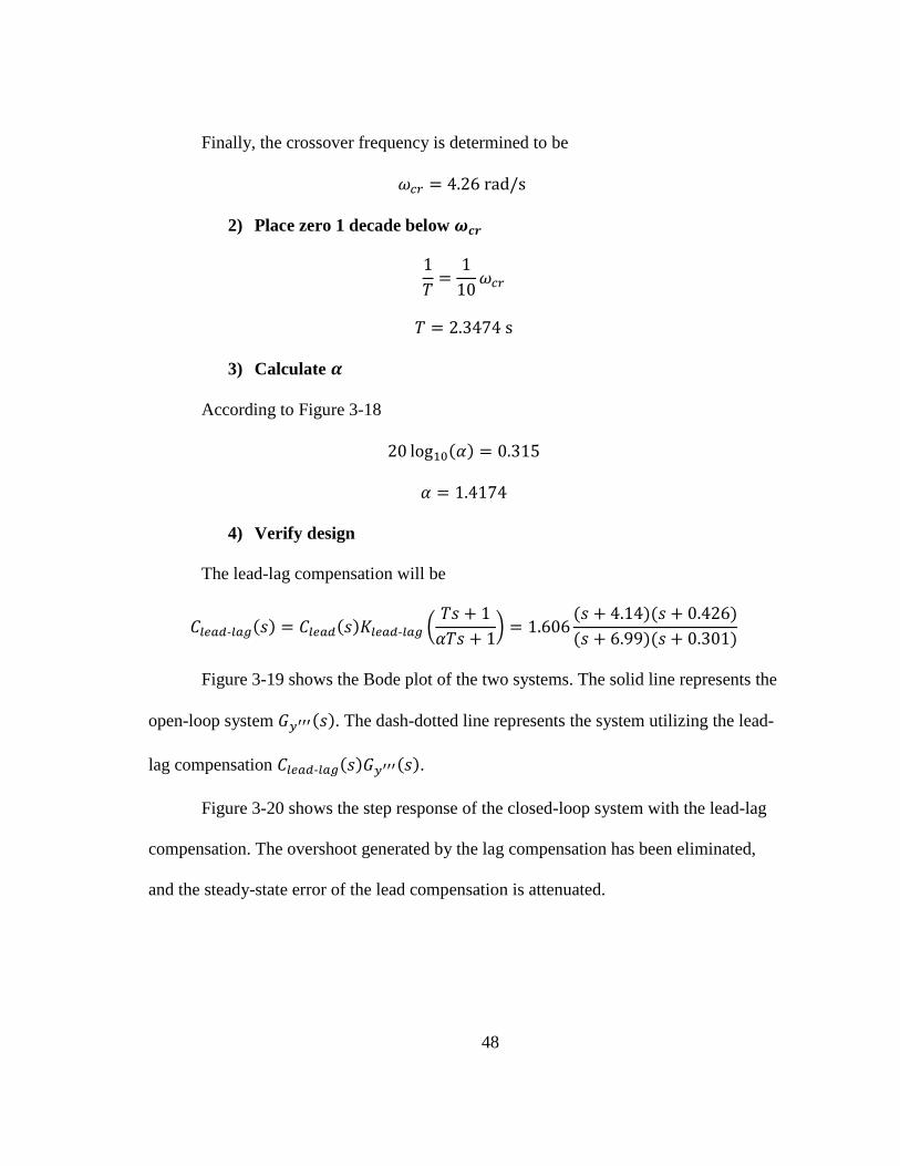
Finally, the crossover frequency is determined to be
𝜔𝑐𝑟 = 4.26 rad/s
2) Place zero 1 decade below 𝝎𝒄𝒓
1
𝑇=
1
10𝜔𝑐𝑟
𝑇 = 2.3474 s
3) Calculate 𝜶
According to Figure 3-18
20 log10(𝛼) = 0.315
𝛼 = 1.4174
4) Verify design
The lead-lag compensation will be
𝐶𝑙𝑒𝑎ⅆ‐𝑙𝑎𝑔(𝑠) = 𝐶𝑙𝑒𝑎ⅆ(𝑠)𝐾𝑙𝑒𝑎ⅆ‐𝑙𝑎𝑔 (𝑇𝑠 + 1
𝛼𝑇𝑠 + 1) = 1.606
(𝑠 + 4.14)(𝑠 + 0.426)
(𝑠 + 6.99)(𝑠 + 0.301)
Figure 3-19 shows the Bode plot of the two systems. The solid line represents the
open-loop system 𝐺𝑦′′′(𝑠). The dash-dotted line represents the system utilizing the lead-
lag compensation 𝐶𝑙𝑒𝑎ⅆ‐𝑙𝑎𝑔(𝑠)𝐺𝑦′′′(𝑠).
Figure 3-20 shows the step response of the closed-loop system with the lead-lag
compensation. The overshoot generated by the lag compensation has been eliminated,
and the steady-state error of the lead compensation is attenuated.

49
Figure 3-19 Bode plot for the lead-lag compensation
Figure 3-20 Step response of the system with lead-lag compensation
3.4 Simulation
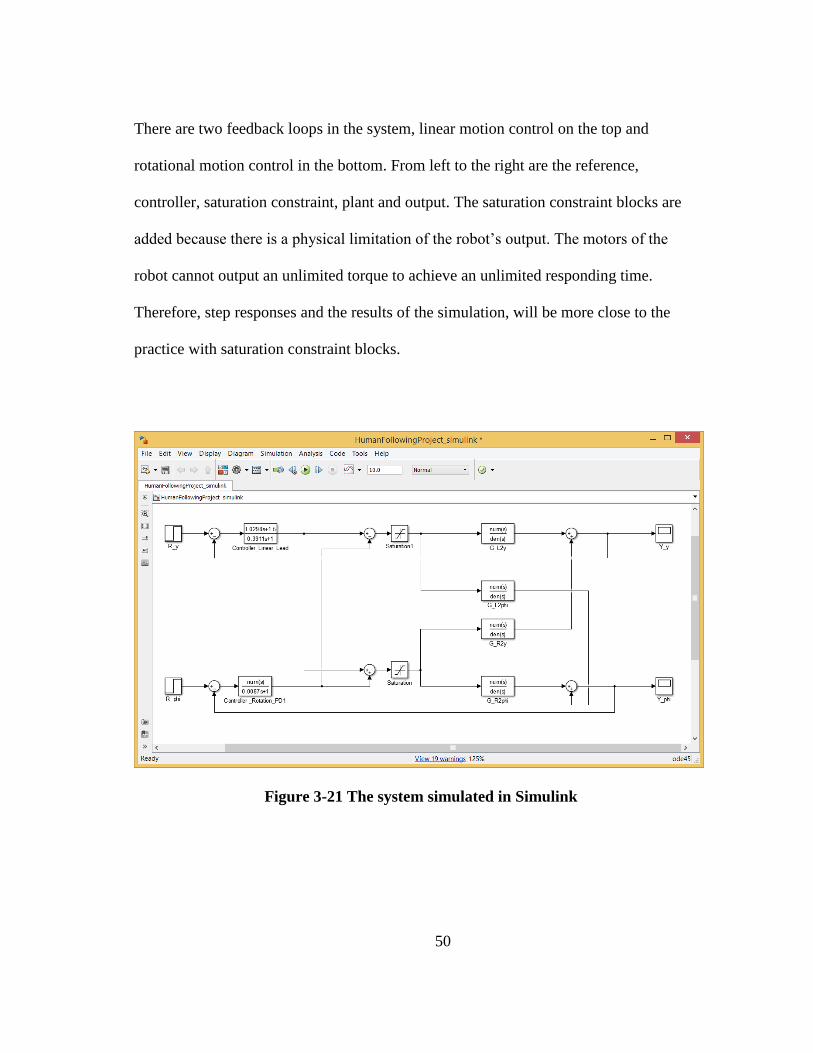
In this section, Simulink is used to simulate the performance of the controllers
designed in the last section. Figure 3-21 is the architecture of the system in Simulink.
50
There are two feedback loops in the system, linear motion control on the top and
rotational motion control in the bottom. From left to the right are the reference,
controller, saturation constraint, plant and output. The saturation constraint blocks are
added because there is a physical limitation of the robot’s output. The motors of the
robot cannot output an unlimited torque to achieve an unlimited responding time.
Therefore, step responses and the results of the simulation, will be more close to the
practice with saturation constraint blocks.
Figure 3-21 The system simulated in Simulink

51
3.4.1 PID controller
Figure 3-22 shows the result of the simulation of the PID controller for linear
motion control. The rise time is about 3 s, which is slightly slower than the previous
analysis (2.3-s rise time), and the steady-state error is about 0.09 m, which is larger than
the previous analysis (0.05-m steady-state error). In the first 2.5 seconds, the response is
linear. This is because it at the robot’s maximum output, and the saturation constraint
block limits the torque output.
Figure 3-22 Simulation result of PID controller for linear motion
Figure 3-23 shows the result of the simulation of the PID controller for rotational
motion control. The result is match the previous analysis well. The rise time is about 2.3
s, and there is with a 0.03° overshoot, which is very small and acceptable.

52
Figure 3-23 Simulation result of PID controller for rotational motion
3.4.2 Lead-lag controller
The simulation result of the system with the lag compensation designed for linear
motion control in the last section is shown in Figure 3-24. With saturation constraint the
steady-state error here is larger than the one analyzed in last section. The steady-state
error is about 0.04 m, which is better than that of the PID controller.
Figure 3-25 is the simulation result of the lead controller for linear motion. The
rise time is about 2.6 s, and the steady-state error is zero, which makes it better than the
other controllers.
Figure 3-26 is the simulation result of the lead-lag controller for linear motion
control. It is similar with the result of the lead controller, which also has a 2.6-s rise time
and zero steady-state error.

53
Figure 3-24 Simulation result of the lag compensation for linear motion
Figure 3-25 Simulation result of the lead compensation for linear motion

54
Figure 3-26 Simulation result of the lead-lag compensation for linear motion
3.5 Technical discussion and evaluation
In this chapter, five controllers were designed, one for the rotation control and
four for the linear motion. For the rotation control, the PID controller is good enough for
the system. It has a tiny overshoot and a short rise time. For the linear-motion control,
the PID controller has a 0.09-m steady-state error, and the lag compensation have a 0.04-
m steady-state error, while the lead and lead-lag controller have a better performance
(2.6-s rise time, no overshoot, and no steady-state error).

55
CHAPTER IV
HUMAN-ROBOT INTERACTION DESIGN
4.
In this chapter, the human-robot interaction system, shown in Figure 4-1, is
presented. There are two modes of the interaction system: the human-tracking mode and
the gesture-control mode. The default mode is the human-tracking mode because it is the
premise for the robot to receive gesture-based commands from the user since the Kinect
sensor has to face the user, and the user should be in the detectable range. In section 4.1
the human-tracking mode is discussed. Section 4.2 elaborates the gesture-control mode.
Start
Tracking mode
Gesture mode
Mode-switch gesture?
Mode-switch gesture?
Figure 4-1 Flowchart of the whole interaction system
Yes
Yes
No
No

56
As shown in Figure 4-1, the system will begin with the human-tracking mode.
Once the system detects the mode-switch gesture, it will shift to gesture-control mode. If
not, it will keep tracking the user. Once the system shifts to the gesture-control mode,
detecting the mode-switch gesture can exit the gesture-control mode.
4.1 Human tracking
In this section, two human-tracking algorithms are developed for the onboard
Kinect sensor and the wide angle camera mounted on the ceiling, respectively. Both data
captured by the Kinect sensor and the camera can be adopted for feedback control loop.
4.1.1 Human tracking with the Kinect sensor
4.1.1.1 Human detection
The human detection based on a Kinect sensor relies upon the OpenNI, a
middleware introduced before, for two reasons. On the one hand, the real capabilities of
the Kinect sensor can be fully assessed, using the framework designed for it. On the
other hand, this approach allows to save time because coding for skeleton tracking is not
necessary with the OpenNI library.
The reference coordinates defined by the Kinect sensor are shown in Figure 4-2.
This is a right-handed coordinate system that place a Kinect at the origin with the
positive z-axis extending in the direction in which the Kinect is facing. The positive y-
axis extends upward, and the positive x-axis extends to the left.
4.1.1.2 Human-tracking
Due to physical limitations, given a mobile robot with a Kinect sensor, only one

57
target can be tracked at a time (although the Kinect sensor is able to track up to six
users). The 3D coordinates of the center of mass of the user is obtained by using a set of
functions provided by OpenNI.
Figure 4-2 Reference coordinates of the Kinect sensor
Once the spatial coordinates of the user are obtained, the distance and angle
offset are need to be computed, in order to run and reorient the mobile robot according to
the motion of the user. In this research, only 2 dimensions are considered (x and z).
Considering the reference coordinate shown in Figure 4-2, and by means of basic
geometry (see Figure 4-3 and Figure 4-4) the absolute distance of the user (neglect y
dimension) calculated as follows:
𝑑𝑎 = (√𝑑𝑥2 + 𝑑𝑧
2 − tan(𝜑𝑘)) cos(𝜑𝑘) (4.22)
Where 𝑑𝑎 is the distance to the user, 𝜑𝑘 is the angle between the center line of the
𝑧
𝑥
𝑦

58
Kinect sensor and the horizontal line, and 𝑑𝑥 and 𝑑𝑧 indicate the distance of the user
along the x- and z-axes. Then the angle between the z-axis and the user 𝜃𝑘 would be
𝜃𝑘 = atan (
𝑑𝑥
𝑑𝑧) (4.2)
Figure 4-3 The top view of the user in the Kinect’s coordinates
A graphical user interface (GUI) was designed, as shown in Figure 4-5, to
indicate the error distance in real time (on the left) and to adjust the reference input by
adjusting a slider (on the right).
User
Kinect
𝑥
𝑧
𝜃𝑘
(𝑑𝑥, 𝑑𝑧)

59
Figure 4-4 The front view of the user in the Kinect’s coordinates
Figure 4-5 Graphical user interface for tracking mode
𝑑𝑎
𝜑𝑘

60
4.1.2 Human tracking with the wide-angle camera
4.1.2.1 Object detection
In this research, the object detection based on the camera is realized by the color
detection function of OpenCV. OpenCV does provide human-tracking algorithm for
developers. However, color detection and tracking is simpler and more reliable.
Therefore, the color tracking function provided by OpenCV is adopted in this research.
To track of the user and the robot by applying the color tracking algorithm only, the user
is asked to put on a cap with specific color, and the robot is decorated with two tapes in
different color. All the colors assigned to the user and the robot are not to be spotted
easily in a lab environment to avoid the camera mistaking other objects as the interested
objects.
4.1.2.2 Human tracking
OpenCV processes images by pixels, so the position of the interested colors also
presented by pixels. For instance, Figure 4-6 is a sample image with frame width W and
frame height H. The positions of the user and the robot are (𝑥𝑡, 𝑦𝑡) and (𝑥𝑟,𝑦𝑟),
respectively. The unit of W, H, 𝑥𝑡, 𝑦𝑡, 𝑥𝑟 and 𝑦𝑟 is pixel. To get a high frame rate, the
frame size is set to 640×480. So the W here is 640 pixels and the H is 480 pixels.
The camera-based human-tracking subsystem runs by a C++ program. In this
program three specific colors are being tracked, the green color of the hat that the user
puts on, the yellow color that decorated on the Kinect sensor, and the pink-color tape
that decorated on the rear of the robot, as shown in Figure 4-7. The figure was captured
by the camera mounted on the ceiling while tracking. The robot and the user was located

61
by two red circles with coordinates beside, and denoted by caption “robot” and “user”
respectively. The program will keep locating these three colors. To calculate the distance
between the user and the robot, the coordinates in pixel should be transformed to be of a
unit of length.
Figure 4-6 A schematic of a camera view
W
H
User
(𝑥𝑡, 𝑦𝑡)
Robot
(𝑥𝑟,𝑦𝑟)
X
Y

62
Figure 4-7 Tracking by the camera
4.1.2.2.1 Distance calculation
Figure 4-8 is a schematic diagram to clarify how a camera captures a picture. The
schematic diagram is drawn as a front view. That means the length of the view here is
related to the width of the frame. To calculate the angle of the view in this direction, the
maximum length of the floor that the camera can capture in the direction related to frame
width is measured as 𝐿𝑓𝑤. The height of the camera (from the floor to the camera) is
measured as 𝐻𝑓.

63
C
12345
12
12
Figure 4-8 A schematic of camera capturing in front view
So the capture angle of the camera in this direction can be calculated by
tan (
𝜃𝑤
2) =
𝐿𝑓𝑤
2𝐻𝑓 (4.3)
Assume that the user is of height 𝐻𝑡. The height from the camera to the user’s hat is
𝐿𝑡 = 𝐻𝑓 − 𝐻𝑡. (4.4)
Then the real length that the camera captures at the height of a user is
𝑙𝑥𝑡
𝑙𝑥𝑟
𝐻𝑓
𝐿𝑡 𝐿𝑟
𝑙𝑥𝑟𝑡
𝐿𝑓𝑤
𝜃𝑤

64
2𝐿𝑡 ⋅ tan (
𝜃𝑤
2). (4.5)
Hence, the actual length from the left edge to the user in the x direction can be calculate
by multiply the maximum length in that height with the percentage of pixel
𝑙𝑥𝑡 = 2𝐿𝑡 tan (
𝜃𝑤
2)
𝑥𝑡
𝑊 . (4.6)
The actual length of the robot in the x direction can be obtained in the same way
𝑙𝑥𝑟 = 2𝐿𝑟 tan (
𝜃𝑤
2)𝑥𝑟
𝑊 . (4.7)
The height of the robot is longer than that of the user, and the coordinate is
calculated from the left edge. So to calculate the distance between the user and the robot
in the x direction, the longer part in the left edge, 𝑙𝑥𝑟𝑡, should be known.
𝑙𝑥𝑟𝑡 = (𝐿𝑟 − 𝐿𝑡) tan (
𝜃𝑤
2) (4.8)
Finally, the distance between the user and the robot in the x direction can be obtained by
𝑙𝑥𝑎 = 𝑙𝑥𝑟 − 𝑙𝑥𝑡 − 𝑙𝑥𝑟𝑡 (4.9)
Figure 4-9 is a left view, so all the horizontal length in the diagram are in the y
direction. All the processes are the same with in the x direction. First, obtain the capture
angle in this direction
tan (
𝜃ℎ
2) =
𝐿𝑓ℎ
2𝐻𝑓 (4.10)
Then calculate the length of the user (𝑙𝑦𝑡) and the robot (𝑙𝑦𝑟) to the left edge in the y
direction.
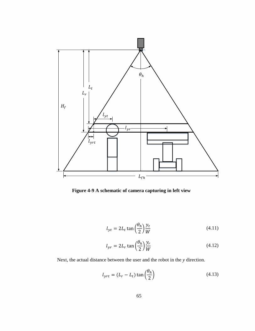
65
C
123456
1231
23
Figure 4-9 A schematic of camera capturing in left view
𝑙𝑦𝑡 = 2𝐿𝑡 tan (
𝜃ℎ
2)
𝑦𝑡
𝑊 (4.11)
𝑙𝑦𝑟 = 2𝐿𝑟 tan (
𝜃ℎ
2)
𝑦𝑟
𝑊 (4.12)
Next, the actual distance between the user and the robot in the y direction.
𝑙𝑦𝑟𝑡 = (𝐿𝑟 − 𝐿𝑡) tan (
𝜃ℎ
2) (4.13)
𝑙𝑦𝑡
𝑙𝑦𝑟
𝐻𝑓
𝐿𝑟
𝐿𝑡
𝑙𝑦𝑟𝑡
𝐿𝑓ℎ
𝜃ℎ

66
𝑙𝑦𝑎 = 𝑙𝑦𝑟 − 𝑙𝑦𝑡 − 𝑙𝑦𝑟𝑡 (4.14)
Finally, the distance between the user and the robot in 2D is
𝑙𝑎 = √𝑙𝑥𝑎
2 + 𝑙𝑦𝑎2 (4.15)
4.1.2.2.2 Angle offset calculation
The angle offset calculation is based on the rule of cosine. There are two points
of the robot being tracked by the camera, the Kinect sensor on the front and the paper
board on the rear, as shown in Figure 4-10. The position of the Kinect sensor is taken as
the position of the robot, and the position of the paper board is to calculate the
orientation of the robot.
According to the rule of cosine, the angle offset 𝜃𝑟𝑡 is given by
𝜃𝑟𝑡 = arccos (
𝑙𝑎2 + 𝑙𝑓𝑟
2 − 𝑙𝑎𝑟2
2𝑙𝑎𝑙𝑓𝑟) (4.16)
4.1.3 The whole process of tracking
There are three individual programs involving the tracking process, the C++
program operating the wide-angle camera, Processing program running the Kinect
sensor, and Arduino program governing the mobile robot. They are shown in the left,
middle, and right columns in Figure 4-11, respectively. To start the system, first power
on the robot, and the Arduino program will run automatically. Second, run the C++
program, and a data communication server will be established. However, at this moment
the camera is not yet tracking. The C++ program will not move to next step until the
Processing program makes a connection to it successfully. Finally, run the Processing

67
program. Once the connection is established, the whole system works normally.
Target
Robot
Figure 4-10 A schematic of camera capturing in top view
For the C++ program, at first, it reads camera calibration data, which are the
output of a camera calibration program. Second, after processing these data, the camera
starts tracking three specific colors and outputs their coordinates in pixel. Third, it
computes the distance and angle between the user and the robot according to the
algorithm discussed above. Forth, it sends these data to the Processing program for
further computation.
𝜃𝑟𝑡
𝑙𝑎
𝑙𝑎𝑟
𝑙𝑓𝑟

68
Start
Run the C++ program to establish a sever
Run the Processing program to connect to
the serve
Connection established?
The camera starts tracking a target and
the mobile robot
Compute distance and angle between the
target and the robot
Send computed data to the Processing
program
Record position data of the target and the robot to a text file
Draw the position of the target and the robot in the screen
Detect human
Decide Target
Obtain target 3D position
Receive data
Compute distance and angle offset
Compute Speed offset base on data both from
the camera and the Kinect
Got data from the C++ Program?
Compute Speed offset base on data both from
the Kinect only
Send velocity offset data to the Arduino
Lost Target?
Power on the robot
Got data?
Run the robot
Wait for data from the Processing program
End
Wait for the Processing program to connect
Undistort the camera
Figure 4-11 Flowchart of the human-tracking system
Fifth, it records the position data of the user and the robot as a text file for further
No
Yes
Yes
Yes
Yes
No
No
No

69
analysis. Sixth, it draws three different color circles in a captured video to indicate the
location of the user and the robot. Then, it goes back and repeats tracking processes.
For the Processing program, after connected to the C++ server, the system will
detect a human within the Kinect sensor’s detectable range. The first detected person
becomes the user to be tracked. Then the processing program obtains the position of the
user’s center of mass. After computing the distance and angle offset, the system
determines whether the C++ program is sending data. If yes, then the system processes
data from both the camera and the Kinect sensor. If not, the system processes data from
the Kinect sensor only. These distance and angle data are processed by one of the
controllers designed in the last chapter to calculate the desired velocity offset for the
robot to track the user. Then these velocity offset data are sent to the Arduino program.
Next, the system checks if the user has lost tracking or not. If the robot lost tracking of
the user, it tries to detect human again. If not, it repeats to obtain the position of the user
and keeps tracking.
For the Arduino program, it just simply waits for the velocity offset data from the
Processing program. Once it receives the data, it runs the robot.
4.2 Gesture control
In chapter Ⅰ, several gesture recognition techniques and applications were
presented. According to the motivations for a user-friendly robot to interact with, in this
chapter, the implementation of the gesture-control system is presented. To achieve a
practical gesture-based interaction system, four gestures are defined, aiming to
implement a vision-based gesture recognizer. Within the whole set of defined gestures,

70
the system is designed to recognize only body gestures since hand gestures are
unrecognizable. Figure 4-12 shows the GUI designed for the gesture-control mode. A
virtual stage, Kinect sensor, and the skeleton of the user are drawn in the program
window.
Figure 4-12 GUI for gesture controlling mode
4.2.1 Skeleton tracking
Figure 4-13 shows the skeleton that the Kinect sensor tracks. The Kinect sensor
tracks all the joints of the body and OpenNI is used as a middleware to access these data.
These date contain geometry information of all the joints of the skeleton.

71
4.2.2 Gesture definition
This section presents the gestures the system is able to recognize. The vocabulary
consists of the four gestures presented below:
Switch to controlling
Switch to tracking
Lamp creation
Lamp selection and color control
Figure 4-13 The Skeleton that the Kinect sensor tracks
Head
Right shoulder
Right elbow
Right hand
Neck
Right hip
Right knee
Right foot Left foot
Left knee
Left hip Left hand
Left elbow
Left shoulder

72
The gestures are defined by stipulating some angles of joints. Part of these
gestures are referred to [22]. The three gestures are just designed to show the robot’s
interaction capability, it is easy to increase the number of recognizable gestures by
adding definitions.
Gesture 1: Switch to controlling
This gesture is used to switch from the tracking mode to the gesture controlling
mode. The gesture requires the user to raise his/her arms laterally. The gesture is chosen
for three reasons: first, it is easy to execute. Second, it is easy to be recognized by the
sensor because there is no overlap of the body. Third, people do not raise their arms that
high while they are walking, so it is hard to be mistaken.
To inform the robot that the user is performing this switch gesture, four angles
of joints are stipulated to be close to 180° (±10°), as shown in Figure 4-14. Therefore,
whenever all these angles are met the requirement of the stipulation, actions of this
mode-switch gesture is triggered.
Gesture 2: Switch to tracking
This gesture is used to switch from the gesture controlling mode to the tracking
mode. The gesture requires that the user expose his/her arms in front of the Kinect
sensor and make them closer.
To inform the robot that the user is performing this switch gesture, the distance
between the user’s hands must be closer than 0.01 m, as shown in Figure 4-15.
Therefore, whenever the distance meets the requirement of the stipulation, actions of this
mode-switch gesture is triggered.
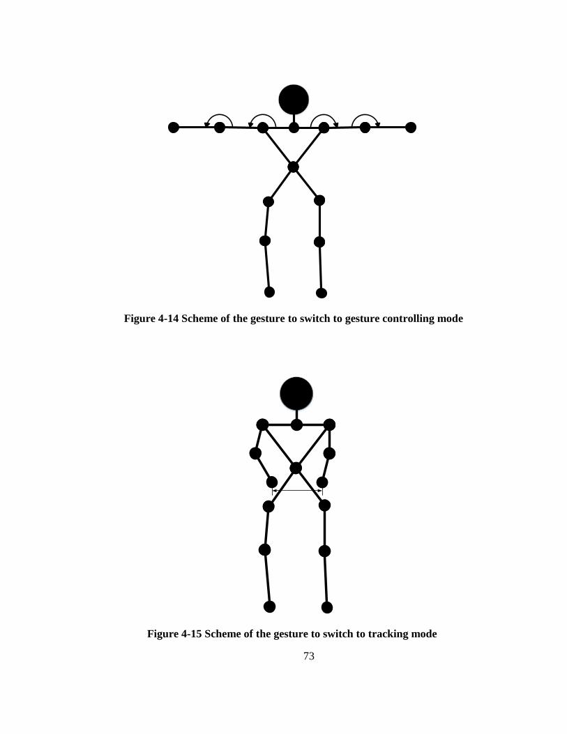
73
Figure 4-14 Scheme of the gesture to switch to gesture controlling mode
Figure 4-15 Scheme of the gesture to switch to tracking mode

74
Gesture 3: Lamp creation
This gesture is to create a virtual lamp in the reference coordinates of the Kinect.
In other words, it is use to tell the Kinect where the lamp is located. Since the object
recognition application has not been added to the system yet, this is a practical way to
locate a lamp in the Kinect coordinates. Once this gesture is recognized, the position of
the center of mass of the user will be recorded and regarded as the position of the lamp,
and a rectangle will be drawn in the GUI window to indicate the location of the lamp.
This gesture requires the user to touch his/her head with hands. To define this
gesture in the program, the distance between each hand to the head of the user will be
evaluated, as shown in Figure 4-16. If the distances are around 0.1 m (±0.05 m), the
lamp creation gesture is triggered.
Figure 4-16 Scheme of the lamp creating gesture

75
Gesture 4: Lamp selection and color control
This gesture is used to tell the robot which lamp the user selected and to change
the color of the lamp. When the system recognizes that the user points to one of the
lamps created before with his/her right hand, the rectangle in the GUI turns white to
indicate that the lamp is selected. In the meantime, the color of that lamp will be
changed according to the height of the user’s left hand.
For this gesture, the user is required to use his/her right hand to point to the
virtual lamp, which is located at the position that the user performed the lamp creation
gesture. To adjust the color of the lamp, the user needs to raise his/her left hand. The
color of the lamp is changed according to the level of the user’s left hand, as shown in
Figure 4-17.
Figure 4-17 Scheme of the lamp selecting and color changing gestures

76
4.2.3 Gesture control
For the gesture-control system, as shown in Figure 4-18, at the beginning, the
system tracks the user’s skeleton. Then the system decides whether the user is
performing the gesture for switching to gesture controlling mode or not. If yes, it
switches to the human-tracking mode. If not, it evaluates specific joint angles and joint
distances to see if the user is touching his/her head or pointing to a lamp. If the user is
touching his/her head, the system creates a virtual lamp at the position of the user’s
center of mass. If the user is pointing to a lamp, it turns white that lamp in the GUI and
changes the color of the lamp based on the level of the user’s left hand.
Start
Track skeleton
Wait for command gestures
Create light
Point a light?
Switch gesture?
Touch head?
Change color of that light
Indicate that light in GUI
Enable target tracking
Figure 4-18 Flowchart of the gesture-control system
No
No
No
Yes
Yes
Yes
77
CHAPTER V
EXPERIMENTAL RESULTS
5.
In this chapter the performance of the robot is evaluated by analyzing the
obtained results. Two types of experiments are performed, in order to evaluate the
following aspects of the robot:
1. Robustness of the human-tracking subsystem
2. Reliability of the gesture-control subsystem
The experimental platform is shown in Figure 5-1. The figure is captured by the
wide-angle camera mounted on the ceiling. The camera is used to capture the position of
the robot and the user. The Kinect sensor was decorated with yellow tape, while the user
to be tracked is asked to put on a green hat. The C++ program was set to track these two
colors. The black marks on the floor are to indicate distance and angle between the user
and the robot. The three marks on the left are to denote the distance (from left to the
right are 2, 1.5 and 1 m, respectively). The four marks on the right are to denote the
angle (from top to the bottom are 20°, 15°, 10°, and 0°). The robot will be placed on
designated mark, and the user is standstill on a designated mark either in every test. In
each of the following experiments, the experimental setup is first detailed and then the
results of the test are discussed.

78
Figure 5-1 Experimental platform
5.1 Human-tracking evaluation
In this section experiments performed on the sole human-tracking subsystem are
presented in order to evaluate the robustness of such system with respect to analyzing
the time response diagrams.
5.1.1 Experimental design
There are four experiments to evaluate the robot’s tracking performance. The
first one is to test the linear motion of the robot exclusively. The second one is to test the
rotational motion of the robot exclusively. The third one is to test both linear motion and
rotational motion at the same time. The fourth one is 2D trajectory tracking. Although

79
the robot is connected to the laptop with wires during the experiments, it can move
freely on the floor, and the influence of the wires is minimal and neglected.
5.1.1.1 Linear motion
For this experiment, a set of tests is carried out to obtain the linear response data
of the four controllers developed in Chapter Ⅲ to various distances. The experiment is
executed with one subject acting as the user to be tracked by the robot. As shown in
Figure 5-2, the robot is placed on the 2-m mark or 1.5-m mark (2-m mark in Figure 5-2)
on the floor of the lab, and facing the 0° mark, while the user is asked to face the robot
and stand still in front of it during the tests.
Figure 5-2 Configuration of the linear motion experiment

80
Each distance is performed four times (performed by four different controllers),
for an overall execution of eight times. During the experiment the distance between the
robot and the user is recorded by both the Kinect sensor and the camera. The reference
distance input is set to be 1 m. Therefore, when the tracking begins, the robot will rush
to the user and then stop at the 1-m mark in front of the user. Since the robot is placed 2
or 1.5 m away from the user, two step responses with amplitude of 1 and 0.5 m are
obtained.
5.1.1.2 Rotational motion
For the rotational motion experiment, a set of tests is carried out to obtain the
rotational response data of the PID controller to different angles. This experiment is also
executed with one user to be tracked by the robot. The robot is placed on 2-m mark, as
shown in Figure 5-3.
The user is asked to stand still in front of the robot on three different marks, 10°,
15° and 20° (15° in Figure 5-3). The test is performed once per angle. During the
experiment the angle between the robot and the user is recorded by the Kinect sensor
only. The reason the angle calculated by the camera is not adopted is it has an error
about 30°, which is unacceptable. The error is large because the two points of the robot
tracked by the camera is too close.
The reference angle input is set to be 0°. Therefore, when the tracking begins, the
robot turns and faces the user straightly. Since the user is standing on the 10°, 15°, or 20°
mark, 3 step responses with the amplitudes of 10°, 15°, and 20° will be obtained.

81
Figure 5-3 Configuration of the rotation experiment
5.1.1.3 Overall performance
In this experiment, two set of tests is carried out to obtain the rotational response
data of the lead and lead-lag controller, respectively. The robot is placed on the 2-m
mark. The user is asked to stand still in front of the robot on the 15° mark. During the
experiment the distance and angle between the robot and the user is recorded by the
Kinect sensor and the camera. The reference angle input is set to be 0°, and the reference
distance input is set to be 1 m. Therefore, when the tracking begins, the robot runs and
turns to the user simultaneously.
5.1.1.4 2D trajectory tracking
This experiment is to show the tracking capability of the robot. The laptop

82
connected to the robot is placed on top of a moveable chair. In order to reduce the
influence of the wire tension to the robot, the chair is moved by a volunteer following
the robot wherever the robot moves. The user is ask to walk randomly within the view of
the wide-angle camera. The robot is set to track the user and maintain a 1-m safe
distance. During the experiment, the positional data of the user and the robot are
recorded by the camera, and Matlab is used to generate trajectories of the user and robot.
5.1.2 Results
In this section the results from the four experiments are presented. The results
from the Kinect sensor alone and from the wide-angle camera are compared in the
linear-motion experiments. The experimental results of the first three experiments are
presented by giving step responses. For the linear-motion control, only results performed
by the lead-lag controller are presented, since it is the best. For the rotational motion
control, all the results are performed by the PID controller, since it is the only controller
developed for the rotational motion. All the responses in time domian are obtained by
Matlab.
5.1.2.1 Linear motion
The experimental result of the linear motion control is presented by collecting
distance data by the wide-angle camera and the Kinect sensor and comparing them with
the simulation result. In this section, each step response consists of three lines. The solid
line represents the distance detected by the wide-angle camera, which is more reliable
and can be considered the real distance. The dash-dotted line represents the distance
detected by the Kinect sensor. The dashed line represents the simulation result.

83
5.1.2.1.1 Performed by the Kinect sensor only
In these set of experiments only the data sent by the Kinect sensor were adopted
for feedback control. The data recorded by the camera are used only as a reference.
Figure 5-4 shows the linear-motion experimental result of the system performed by the
Kinect sensor (the camera is not included in the feedback loop) with initial distance at 1
m.
Figure 5-4 Experimental result of the lead-lag controller (1 m)
In the first 3.3 seconds, the experimental result match well with the simulation
result. After 3.3 s, there is a small error (about 0.001 m) of the data captured by the
84
Kinect sensor. The Kinect sensor locates the center of mass of the user actually.
However, it cannot calculate the precise potion of the user sometime while it is too close
to the user and cannot capture the whole body of the user. Apart from this error,
comparing the data of the Kinect to the simulation result, there is a small error as well.
The error is caused by the physical limitation of the robot’s hardware. Since there is a
dead-zone in the torque output of the robot due to friction, the robot would not move if
the duty ratio of the PWM signal is smaller than 5%. However, a 0.05-m steady-state
error is acceptable for tracking in our application.
Figure 5-5 shows the linear motion experimental result of the system performed
by the Kinect sensor with initial distance at 0.5 m. As shown in the figure, there is some
delay and small oscillations (range of 0.04 m) between 2–3 s. Actually, the robot was not
shaking, the oscillations is generated by the method accessing to the position of the user.
5.1.2.1.2 Performed by the wide-angle camera
In this set of experiments only the data captured by the camera is adopted for
feedback control. The data recorded by the Kinect sensor are used only as a reference.
Figure 5-6 shows the linear-motion experimental result of the system performed
by the camera with the initial distance at 1 m. The experimental result match with the
simulation result well, with little delay (0.3 s), which may be caused by the uncertainty
of the system including the friction between the wheels and the lab floor.
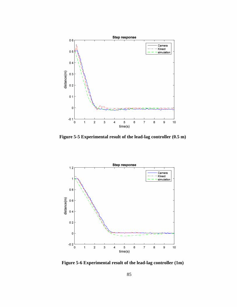
85
Figure 5-5 Experimental result of the lead-lag controller (0.5 m)
Figure 5-6 Experimental result of the lead-lag controller (1m)

86
Figure 5-7 shows the linear-motion experimental result of the system performed
by the camera with the initial distance at 0.5 m. As shown in the figure, the experimental
result matches the simulation result well, except small oscillations occurring in 4–10 s,
which is of the range of 0.03 m. The oscillations are caused by the motion of the user,
since no one can really stand still. One may also find that there is a small delay in the
response of the camera, compared with the response recorded by the Kinect sensor.
Actually, the delay was caused by the communication between the Processing program
and the C++ program. The C++ program records the data captured by the camera and
then sends them to the Processing program, and then combines them with the data
recorded by the Kinect sensor. Therefore, sometimes there is a small delay in the
camera’s data.
Figure 5-7 Experimental result of the lead-lag controller (0.5m)

87
5.1.2.2 Rotational motion
After initial tests, it turned out that the angle calculated by the camera’s data was
not precise for steering. This error was more than 30°. The reason for the error is that the
two points of the robot chosen for tracking is too close. Therefore in this section, the
angle data from the camera are eliminated. The dashed line denotes the data recorded by
the Kinect sensor, and the solid line represents the simulation result.
Figure 5-8 shows the rotation experimental result performed by the Kinect sensor
with the initial angle of 10°. There were some delay and a small overshoot, but the
steady-state error was quite small (about 0.3°). The experimental result of the system for
15° rotation is shown in Figure 5-9. There is a 0.2-s delay, while the steady-state error
are still small.
Figure 5-8 Experimental result of the PID controller for rotation (10°)

88
Figure 5-9 Experimental result of the PID controller for rotation (15°)
Figure 5-10 shows the experimental result of the system for 20° rotation. There is
still a 0.2-0.3-s delay. The delay of the rotation maybe caused by the uncertainty of the
system including the friction between the wheels and the lab floor.
For the rotational motion experiments, the results shares common phenomena,
small response delay (about 0.2 s) and very small steady-state error (smaller than 1°).
Tests proved that the small delay does not affect tracking.

89
Figure 5-10 Experimental result of the PID controller for rotation (20°)
5.1.2.3 Combined experiments
In this section, experimental results with two initial angles 10° and 15° are given.
For each test, a step response of distance and a step response of angle are shown. The
Kinect is the only sensor included in the feedback control loop, while the camera is used
only for reference. The lead-lag controller is used for linear motion control, and the PID
controller is used for rotational motion control.
Figure 5-11 shows the distance response of the system with initial distance of 1
m and initial angle of 10°. The experimental result matches the simulation result well,
with a small delay (about 0.4 s) and a small steady-state error (about 0.04 m).

90
Figure 5-11 Experimental result of the combined performance with the initial
distance of 1 m and initial angle of 10° (distance response)
Figure 5-12 shows the angle response of the system with initial distance of 1 m
and initial angle of 10°. The experimental result matches the simulation result well, with
a small delay (about 0.4 s) and small oscillations.
Figure 5-13 shows the distance response of the system with initial distance of 1
m and initial angle of 15°. The experimental result matches the simulation result well,
with a small delay (about 0.4 s) and a small steady-state error (about 0.04 m).

91
Figure 5-12 Experimental result of the combined performance with the initial
distance of 1 m and the initial angle of 10° (angle response)
Figure 5-14 shows the angle response of the system with initial distance of 1 m
and initial angle of 10°. The experimental result matches the simulation result well, with
a delay (about 0.5 s at maximum) and small oscillations. Although the results in this set
of experiments does not fit the simulation result perfectly, tests show that these delays
and steady-state errors are acceptable.
To ensure the delays and steady-state errors occurring in tracking are acceptable,
experiments to determine the range of the distance and the angle between the robot and
the user were carried out. The range of the distance was about 0.8–1.8 m, and the range
of the angle was ±18°. Hence, the delays and steady-state errors are acceptable since
they do not drive the robot out of the controllable range.

92
Figure 5-13 Experimental result of combination performance with the initial
distance of 1 m and the initial angle of 15° (distance response)
Figure 5-14 Experimental result of the combined performance with the initial
distance of 1 m and the initial angle of 15° (angle response)

93
5.1.2.4 2D trajectory tracking
Figure 5-15 shows the trajectories of the robot and the user captured by the
camera. The positional data were processed by Matlab. There are 181 data points for
each trajectory adopted for this plot. The camera captures positional data at 30 FPS.
Therefore, the duration of the trajectories should be 6 s. There are markers of 0.5-s
intervals on the trajectories. Recall the reference coordinates of the Kinect sensor given
in Figure 4-2. The displacements in the z-axis (longitudinal direction of the robot) are
clearly shown in the trajectories. In contrast, the displacements in the x-axis are not
conspicuous, since the angular displacements of the robot cannot be represented in this
trajectories.
Figure 5-15 Trajectories of the robot and the user
5.2 Gesture recognition evaluation
This section is dedicated to the experiments executed to assess the reliability of

94
the gesture-recognition subsystem through the assessment of the recognition success rate
with respect to the four gestures presented in Chapter Ⅳ, two mode-switch gestures, and
a lamp creation gesture, lamp selection and color change gesture.
5.2.1 Experimental design
For these tests, ten people, aged 26 years old on average, were asked to perform
all the gestures that the robot is able to recognize. The pool of the ten people consisted of
six males and four females, who had no previous experience either the Kinect or motion
capture. Each experiment is articulated as follows.
The robot is placed on the floor, and the human-tracking system is disabled.
Subject training: first, the subjects learns the gesture vocabularies and
understands how to execute each of them. Then, they perform a training run
consisting of eight executions, two for each gesture;
Evaluation run: this step consists of 12 executions, three for each gesture.
The subjects are asked to perform one of the three gestures, in order for the
calculation of the recognition success rate without any memory effect,
which can affect the evaluation.
5.2.2 Results
Table 5.1 shows the experimental results of the gesture recognition. It is the
average success rates of the individual testing from 1.5 or 2 m away. Every gesture was
recognized well in 0° and 10°. When the test goes to 15° all the success rates of gestures
decreased in different percentages. When it went to 20°, the user was out of the Kinect’s

95
detectable range. For the test from 2 m away, every gesture was recognized well in 0°
and 10°. As the angle increased from 10° to 20°, the success rates of all the gestures
decreased in different percentages. The reason that the success-rate decrease was that the
Kinect sensor could not track the crucial part of the body that triggered the motion. In
other words, the critical body part was out of the Kinect sensor’s best detectable range.
According to these data, when the robot is serving in a distance between 1.5 to 2 m, the
user was not supposed to have an angle more than 20° about the robot.
Table 5.1 Success rate of the gesture recognition
1.5 m 2 m
0° 10° 15° 20° 0° 10° 15° 20°
Mode-switch 1 100% 100% 83% NA 100% 100% 93% 83%
Mode-switch 2 100% 100% 90% NA 100% 100% 100% 93%
Lamp creation 100% 100% 87% NA 100% 100% 97% 90%
Lamp selection 100% 100% 80% NA 100% 100% 93% 83%
Color change 100% 100% 93% NA 100% 100% 100% 93%

96
CHAPTER VI
CONCLUSIONS AND FUTURE WORK
6.
6.1 Conclusions
The challenging aim of natural human-robot interaction (NHRI) is to design
desirable robotic platforms, which can be mass-consumption products. The existing
device with NHRI function can be classified into two groups based on the type of users.
The first group of devices was designed for the general public. Usually, these devices
have very limited function and are unmovable and affordable. For example, the Kinect
for the Xbox 360 console. The Kinect sensor here is just an input for the video game
console. It cannot be used for other devices since it is unmovable. The other group of
devices was designed for specialists and is unsuitable for inexperienced operators. These
devices are usually used in special scenarios, like in an earthquake site or in a laboratory.
They are high-tech, expensive, and unaffordable in general.
The affordable and reliable robotic system developed in this research achieved
the goal that has the potential for wide usage and easy to interface. First, the robot
showed its ability to interact with other electrical devices wirelessly. In the research, this
ability was demonstrated by controlling lamps’ power and their color. Besides, the
robot’s human-tracking ability was evaluated in Chapter Ⅴ, and showed it was robust
within the detectable range of the Kinect sensor. Therefore, with wireless
communication module, the robot could control most of electrical devices.

97
Second, a natural interface means less human effort needed for the interaction,
for example, minimizing the complexity of the user interfaces. To this end, in this work
a new approach for a mobile social robot was proposed, which provided the user a more
natural communication interface. This was achieved without any wearable or graspable
input device, rather equipping a robot with a motion sensor, and a vision-based gesture-
driven interaction system. In addition, the interaction was quite simple and easy.
Experiments in Chapter Ⅴ confirmed the achievement of a gesture-driven interaction
system usable by non-expert operators, which was one aims of the work. Moreover, in
the research, the robot also showed its ability to acquire geometrical data. This means it
may understand what you need before you “tell” it, and do what it can do. For example,
in the research the robot turned on the lamp that the user came close to, and turned off
the lamp that the user went away from. Gesturing is an easy and expressive way people
communicate. Hence, a gesture-driven vision-based interaction system is an optimal
choice for the purpose of developing a socially interactive robot.
Third, it is a potential mass-consumption product, for its low cost. The most
expensive part of the robot is the Kinect sensor, which cost 249 US dollars.
In summary, the implementation of a friendly social robot exhibits good
performances with respect to the objects presented in Chapter I.
6.2 Future work
Although the goals were accomplished, the approach detailed in this thesis
presents some aspects that can be implemented as future work.
First, there is a motor in the Kinect sensor to control the pan-tilt. However, it was

98
not used in the research since the framework of the motor was not yet released for
Windows operating system. The Kinect sensor can always have a best view of the user
by controlling the pan-tilt. Therefore, to make gesture recognition more robust, the best
solution is to enable the pan-tilt.
Second, object recognition was not included in the research. The framework used
for the Kinect is OpenNI, which is not support for object recognition. In the future, other
frameworks may be utilized to implement object recognition, which will facilitate the
human-robot interaction.
Third, it would be interesting to integrate additional human-oriented perception
systems, for example, speech recognition. In this case, one could take advantage of the
hardware already installed on the robot, the array of microphones of the Kinect.
Finally, the Kinect sensor is required to connect to a computer directly with the
USB cable, without any wireless solution. That is why in this research the robot ran with
a wire connected to a laptop. To increase the mobility of the robot, a single-board
computer can be installed on the robot, such as Raspberry Pi. The Raspberry Pi is of
about the same size with an Arduino board, and has been proved to cope with Kinect
Sensor.

99
REFERENCES
[1] J. Chen, “Ultrasonic-based human-tracking mobile robot,” B.S. thesis, Shenzhen
University, Shenzhen, China, May 2012.
[2] B. J. Southwell and G. Fang, “Human object recognition using colour and depth
information from an RGB-D Kinect sensor,” International Journal of Advanced
Robotic Systems, vol. 10, pp. 171, Oct. 2013.
[3] T. Nakamura, “Real-time 3-D object tracking using Kinect sensor,” in Proc. of IEEE
International Conference on Robotics and Biomimetics (ROBIO), Dec. 2011, pp.784–
788.
[4] K. D. Mankoff and T. A. Russo, “The Kinect: a low-cost, high-resolution, short-range
3D camera,” Earth Surf. Process. Landforms, vol. 38, no. 9, pp. 926–936, Jul. 2013.
[5] J. Falconer. (2012). “Smart insect”: Toyota’s cloud-enabled, single-passenger electric
vehicle [Online]. Available: http://www.gizmag.com
[6] M. Raibert, K. Blankespoor, G. Nelson, and R. Playter. (2008). Bigdog, the rough-
terrain quaduped robot [Online]. Available: http://www.bostondynamics.com
[7] Hillcrest. (2012). Hillcrest’s Freespace motion-engine used in TCL’s first domestic
Android-based smart TVs and motion sensing remotes [Online]. Available:
http://www.hillcrestlabs.com
[8] Project Tango. (2014). [Online]. Available: https://www.google.com/atap/project-
tango/
[9] J. Yi, D. Song, J. Zhang, and Z. Goodwin, “Adaptive trajectory tracking control of
skid-steered mobile robots,” in Proc. of IEEE International Conference on Robotics

100
and Automation, April 2007, pp. 2605–2610.
[10] H. Wang, B. Li, J. Liu, Y. Yang, and Y. Zhang, “Dynamic modeling and analysis of
wheel skid steered mobile robots with the different angular velocities of four
wheels,” in Proc. of 2011 30th Chinese Control Conference (CCC), July 2011, pp.
3919–3924.
[11] A. Mandow, J. L. Martinez, J. Morales, J. L. Blanco, A. Garcia-Cerezo, and J.
Gonzalez, “Experimental kinematics for wheeled skid-steer mobile robots,” in Proc.
of IEEE/RSJ International Conference on Intelligent Robots and Systems, Nov. 2007,
pp. 1222–1227.
[12] W. Yu, O. Chuy, E. G. Collins, Jr., and P. Hollis, “Dynamic modeling of a skid-
steered wheeled vehicle with experimental verification,” in Proc. of IEEE/RSJ
International Conference on Intelligent Robots and Systems, Oct. 2009, pp. 4212–
4219.
[13] X. Ha, C. Ha, and J. Lee, “Fuzzy vector field orientation feedback control-based slip
compensation for trajectory tracking control of a four track wheel skid-steered
mobile robot,” International Journal of Advanced Robotic Systems, vol. 10, pp. 218,
Mar. 2013.
[14] E. Hwang, H. Kang, C. Hyun, and M. Park, “Robust backstepping control based on
a Lyapunov redesign for skid-steered wheeled mobile robots,” International Journal
of Advanced Robotic Systems, vol. 10, pp. 26, Oct. 2013.
[15] R. Marcovitz, “On-line mobile robotic dynamic modeling using integrated
perturbative dynamics,” M.S. thesis, the Robotics Institute, Carnegie Mellon

101
University, Pittsburgh, PA, April 2010.
[16] K. Kozlowski and D. Pazderski, “Modeling and control of a 4-wheel skidsteering
mobile robot,” International Journal of Applied Mathematics and Computer Science,
vol. 14, no. 4, pp. 477–496, 2004.
[17] N. Michael, S. Shen, K. Mohta, Y. Mulgaonkar, K. V. K. Nagatani, Y. Okada, S.
Kiribayashi, K. Otake, K. Yoshida, K. Ohno, E. Takeuchi, and S. Tadokoro,
“Collaborative mapping of an earthquake-damaged building via ground and aerial
robots,” Journal of Field Robotics, vol. 29, no. 5, pp. 832–841, Oct. 2012.
[18] S. Long, N. Sünderhauf, P. Neubert, S. Drews, and P. Protzel, “Autonomous corridor
flight of a UAV using a low-cost and light-weight RGB-D camera,” in Proc. of
International Symposium on Autonomous Mini Robots for Research and
Edutainment (Amirs), Bielefeld, Germany, May 2011, pp. 183–192.
[19] ELP. (2015). USB2.0 5MP USB camera module OV5640 color CMOS sensor 3.6 mm
lens [Online]. Available: http://www.elpcctv.com/
[20] OpenNI. (2015). [Online]. Available: http://structure.io/openni
[21] Arduino. (2015). What is Arduino? [Online]. Available: https://www.arduino.cc
[22] E. R. Melgar, Arduino and Kinect Projects: Design, Build, Blow Their Minds, USA:
Apress, 2012, ch. 7, pp. 133–165.

102
APPENDIX
Processing Code
import SimpleOpenNI.*; import processing.serial.*; import controlP5.*; import peasy.test.*; import peasy.org.apache.commons.math.*; import peasy.*; import peasy.org.apache.commons.math.geometry.*; import processing.opengl.*; import processing.net.*; SimpleOpenNI context; //for SimpleOpenNI library Serial myPort4Robot; //for Serial communication Serial myPort4Lamp; ControlP5 cp5; //for user interface Chart myChart; Slider Slider1; File lampsFile; //for lamp control PeasyCam cam; //for 3D present Client c; //for socket communication String n1; // signs and numbers to send to Arduino board String n2; String n3; String n4; String sending; // combined n1, n2, n3, n4 PrintWriter output; // will show on the screen int v; int vl; // velocity of the left wheel int vr; // velocity of the right wheel int y; // distance between a target and robot double theta; // angle between a target and robot int ey1 = 0; // distance error int ey2; // new distance error double etheta1 = 0; // angular error double etheta2; // new angular error int u1 = 0; int u2 = 0; int u3 = 0; int Ry = 1500;//reference y int Rtheta = 0;//reference theta double k = 0.0285; //1*gr*kt*ki=2*120*0.0865*(0.35/255)=0.0285 double kY = 0.033; double kPhi = 1.25; int maxY = 255; // maximum velocity output

103
int maxPhi = 150; // maximum angular output int maxV = 255; int minRun = 10; // minimum velocity output of the robot int dl = 1; //direction of left motor, dl=1 means go forward int dr = 0; //direction of right motor, dr =0 means go forward int mode = 0; // mode1 is tracking, mode2 is gesture control ArrayList<Lamp> lamps = new ArrayList<Lamp>(); // for saving lamps int boundSize = 2400; // for the 3D PeasyCam String input; // for socket communication int data[]; // for user tracking PVector bodyCenter = new PVector(); PVector bodyDir = new PVector(); PVector com = new PVector(); PVector com2d = new PVector(); color[] userClr = new color[]{ color(255,0,0), color(0,255,0), color(0,0,255), color(255,255,0), color(255,0,255), color(0,255,255) }; // for slider in the UI int sliderTicks1 = 100; PFont f; //Declare PFont variable /////////////////////////////////////////////// void setup(){ size(1024,768,P3D); // size of the image context = new SimpleOpenNI (this); // check the connection to Kinect sensor if(context.isInit() == false){ println("Maybe your Kinect is not connected"); exit(); return; } context.setMirror(false); // disable mirror context.enableDepth(); // enable depth sensing context.enableUser(); // enable skeleton tracking //setup PeasyCam cam = new PeasyCam(this, 0, 0, 0, 3500); stroke(255,255,255); smooth(); // frameRate(30); //set framerate //Initialize Serial Communication String port4Robot = Serial.list()[0];

104
String port4Lamp = Serial.list()[1]; myPort4Robot= new Serial(this, port4Robot, 9600); myPort4Lamp = new Serial(this, port4Lamp, 9600); //CP5 PFont pfont = createFont("Arial",10,true); // use true/false for smooth/no-smooth ControlFont font = new ControlFont(pfont,300); //Initialize Control Slider cp5 = new ControlP5(this); cp5.addFrameRate() .setInterval(10) .setPosition(0,height - 10) .setSize(300,300) .setFont(font); Slider1 = cp5.addSlider("Desired Distance") .setPosition(800,150) .setSize(60,400) .setRange(800,1200) .setNumberOfTickMarks(9) ; Slider1.captionLabel() .setFont(font) .setSize(20) .toUpperCase(false) ; Slider1.valueLabel() .setFont(font) .setSize(20) .toUpperCase(false) ; //Initialize Chart myChart = cp5.addChart("Error") .setPosition(150, 150) .setSize(60, 400) .setRange(-80, 80) .setView(Chart.BAR) // use Chart.LINE, Chart.PIE, Chart.AREA, Chart.BAR_CENTERED .setStrokeWeight(1.5) .setColorCaptionLabel(color(40)) ; myChart.captionLabel() .setFont(font) .setSize(20) .toUpperCase(false) ; myChart.addDataSet("distanceError"); myChart.setData("distanceError", new float[1]); cp5.setAutoDraw(false);

105
f = createFont("Arial",128,true); //Initialize Text output = createWriter("Kinect.txt"); // Create a new file to save the position of the target c = new Client(this, "136.0.0.1", 15935); // server's IP and port } /////////////////////////////////////////////// void draw(){ context.update(); // update the cam background(0,0,0); // background color int [] userList = context.getUsers(); // detect humans using Kinect // tracking or gesture control? if (mode==0){ if (c.available() > 0) { input = c.readString(); input = input.substring(0, input.indexOf("\n")); // Only up to the newline data = int(split(input, ' ')); // Split values into an array } if(context.isTrackingSkeleton(1)){ //Displaying text textFont(f,128); fill(0,255,255); textAlign(CENTER); text("You are being tracked.",width/2,height-1000); context.getCoM(1,com); //get the center of mass of the target calculation(com,data[0],data[1]); // calculate the distance and angle offset and send command to the Arduino board gui(); // show the GUI output.println(com.x+","+com.y+","+com.z+","+data[0]+","+data[1]); // Write the coordinate to the file // println("Position:"+com.x+","+com.y+","+com.z+","+data[0]+","+data[1]); } } else if (mode==1){ modeCheck4Gesture(1); // check if it is needed to shift to tracking mode // Draw the stage pushMatrix(); translate(0, 0, boundSize/2); stroke(255, 0, 255); //stroke(50,200); noFill(); box(boundSize); popMatrix(); pushMatrix(); translate(0, boundSize/4, boundSize/2); rotateX(PI/2); stroke(255, 0, 255); noFill(); rectMode(CENTER); rect(0,0,boundSize,boundSize);

106
popMatrix(); ///////////////////////////////flip pushMatrix(); scale(-1,1,1); scale(0.5); rotateZ(radians(180)); rotateY(radians(360)); //image(context.userImage(),0,0); if (context.getNumberOfUsers() != 0) { context.getCoM(1, com); // Get the Center of Mass for (int i = 0; i < lamps.size(); i++) { lamps.get(i).updateUserPos(com); // Update the lamps } userControl(1); // User control behaviors drawSkeleton(1); stroke(100,255,0); strokeWeight(1); beginShape(LINES); vertex(com.x - 15,com.y,com.z); vertex(com.x + 15,com.y,com.z); vertex(com.x,com.y - 15,com.z); vertex(com.x,com.y + 15,com.z); vertex(com.x,com.y,com.z - 15); vertex(com.x,com.y,com.z + 15); endShape(); } for (int i = 0; i < lamps.size(); i++) { lamps.get(i).draw(); } sendSerialData(); // send command to lamps // modeCheck(1); // draw the kinect cam context.drawCamFrustum(); //Draw 3D PeasyCam popMatrix(); } } //distance and orientation caltulation void calculation(PVector com, int data1, int data2) { point(com.x,com.y,com.z); if (com.z < 600) { vl = 0; vr = 0; println("Stop"); } else

107
{ double ratio = -com.x/com.z; double theta = Math.toDegrees(Math.atan(ratio));//new theta println(theta); y = (int)(sqrt(com.z*com.z+com.x*com.x-640000)*0.1+0.9*data1); //new y, adjust the ratio to adjust the weight of the Kinect and the camera int ey2 = y-Ry; //error of distance myChart.push("distanceError", (ey2)); // update chart //Displaying error textFont(f,256); fill(0,255,255); textAlign(CENTER); float ey22 = ey2; text("Distance Error\n"+ey22/1000+"m",65,430); double etheta2 = Rtheta-theta; //error of theta
ut1 = 1.904*ut11-0.9052*ut111+2.44*ey3-4.713*ey2+2.275*ey1; //new model u1 Lead-lag controller, k=1.4, 0.015
ut2 = -0.3038*ut2+0.5004*etheta2-0.1351*etheta1; //update u2 sisotool
// transfer the input from torque to velocity value u1 = (int)(ut1*kY/k); u2 = (int)(ut2*kPhi/k); println("u1:"+u1); println("u2:"+u2); // include physical limitation (maximum speed and maximum detectable angle) if (abs(u1) > maxY) { u1 = (int)(Math.signum(u1)*maxY); } if (abs(u2) > maxPhi) { u2 = (int)(Math.signum(u2)*maxPhi); } println("u12:"+u1); println("u22:"+u2); //calculate the velocity to wheels on each side vl = u1-u2; vr = u1+u2; // determine the wheel's rotate direction if (vl > 0) { dl = 1; } else {

108
dl = 0; vl = -vl; } if (vr > 0) { dr = 0; } else { dr = 1; vr = -vr; } // include physical limitation (maximum speed and maximum detectable angle) if (vl>maxV || vr>maxV) { int u11 = round(u1/(abs((float)u1)+abs((float)u2))*maxV); int u22 = round(u2/(abs((float)u1)+abs((float)u2))*maxV); if (abs(u22)>maxPhi) { u22 = (int)(Math.signum(u22)*maxPhi); u11 = (int)(Math.signum(u11)*(maxV-maxPhi)); if (u11 > u1) u11 = u1; } else if (abs(u11)>maxY) { u11 = (int)(Math.signum(u11)*maxY); u22 = (int)(Math.signum(u22)*(maxV-Y)); if (u22 > u2) u22 = u2; } //calculate the velocity to wheels on each side vl = round(u11-u22); vr = round(u11+u22); } ey1 = ey2; //old ey ey2 = ey3; ut111 = ut11; ut11 = ut1; etheta1 = etheta2;//old theta } modeCheck4Tracking(1); // check mode shift request // transform interger into string n1 = Integer.toString(dl); n2 = Integer.toString(vl); n3 = Integer.toString(dr); n4 = Integer.toString(vr);

109
// if n2 or n4 is less than 4 digits add a zero to the front of them. while (n2.length() < 3){ n2 = '0' + n2; } while (n4.length() < 3){ n4 = '0' + n4; } sending = n1 + n2 + n3 + n4; //combine the four strings into one 8 digit one myPort4Robot.write(sending); //write this to the serial port. } // draw the skeleton with the selected joints void drawSkeleton(int userId) { strokeWeight(5); // to get the 3d joint data drawLimb(userId, SimpleOpenNI.SKEL_HEAD, SimpleOpenNI.SKEL_NECK); drawLimb(userId, SimpleOpenNI.SKEL_NECK, SimpleOpenNI.SKEL_LEFT_SHOULDER); drawLimb(userId, SimpleOpenNI.SKEL_LEFT_SHOULDER, SimpleOpenNI.SKEL_LEFT_ELBOW); drawLimb(userId, SimpleOpenNI.SKEL_LEFT_ELBOW, SimpleOpenNI.SKEL_LEFT_HAND); drawLimb(userId, SimpleOpenNI.SKEL_NECK, SimpleOpenNI.SKEL_RIGHT_SHOULDER); drawLimb(userId, SimpleOpenNI.SKEL_RIGHT_SHOULDER, SimpleOpenNI.SKEL_RIGHT_ELBOW); drawLimb(userId, SimpleOpenNI.SKEL_RIGHT_ELBOW, SimpleOpenNI.SKEL_RIGHT_HAND); drawLimb(userId, SimpleOpenNI.SKEL_LEFT_SHOULDER, SimpleOpenNI.SKEL_TORSO); drawLimb(userId, SimpleOpenNI.SKEL_RIGHT_SHOULDER, SimpleOpenNI.SKEL_TORSO); drawLimb(userId, SimpleOpenNI.SKEL_TORSO, SimpleOpenNI.SKEL_LEFT_HIP); drawLimb(userId, SimpleOpenNI.SKEL_LEFT_HIP, SimpleOpenNI.SKEL_LEFT_KNEE); drawLimb(userId, SimpleOpenNI.SKEL_LEFT_KNEE, SimpleOpenNI.SKEL_LEFT_FOOT); drawLimb(userId, SimpleOpenNI.SKEL_TORSO, SimpleOpenNI.SKEL_RIGHT_HIP); drawLimb(userId, SimpleOpenNI.SKEL_RIGHT_HIP, SimpleOpenNI.SKEL_RIGHT_KNEE); drawLimb(userId, SimpleOpenNI.SKEL_RIGHT_KNEE, SimpleOpenNI.SKEL_RIGHT_FOOT); // draw body direction getBodyDirection(userId,bodyCenter,bodyDir); bodyDir.mult(200); // 200mm length bodyDir.add(bodyCenter); stroke(255,200,200); line(bodyCenter.x,bodyCenter.y,bodyCenter.z, bodyDir.x ,bodyDir.y,bodyDir.z);

110
PVector joint_HEAD = new PVector(); context.getJointPositionSkeleton(userId, SimpleOpenNI.SKEL_HEAD, joint_HEAD); strokeWeight(50); stroke(255); point(joint_HEAD.x, joint_HEAD.y, joint_HEAD.z); strokeWeight(1); } void drawLimb(int userId,int jointType1,int jointType2) { PVector jointPos1 = new PVector(); PVector jointPos2 = new PVector(); float confidence; // draw the joint position confidence = context.getJointPositionSkeleton(userId,jointType1,jointPos1); confidence = context.getJointPositionSkeleton(userId,jointType2,jointPos2); stroke(0,255,255,confidence * 200 + 55); line(jointPos1.x,jointPos1.y,jointPos1.z, jointPos2.x,jointPos2.y,jointPos2.z); } // mode shift from tracking to controlling public void modeCheck4Tracking(int userId) { // Hand Vectors PVector rHand = new PVector(); PVector lHand = new PVector(); context.getJointPositionSkeleton(userId, SimpleOpenNI.SKEL_RIGHT_HAND, rHand); context.getJointPositionSkeleton(userId, SimpleOpenNI.SKEL_LEFT_HAND, lHand); // if distance between both hand samller than 0.08m then shift to controlling mode if (lHand.dist(rHand) < 80){ vl = 0; vr = 0; mode = 1; } } // mode shift from controlling to tracking public void modeCheck4Gesture(int userId) { // define joints Vectors PVector lHand = new PVector(); PVector lElbow = new PVector(); PVector rShoulder = new PVector(); PVector lShoulder = new PVector(); context.getJointPositionSkeleton(userId, SimpleOpenNI.SKEL_LEFT_HAND, lHand); context.getJointPositionSkeleton(userId, SimpleOpenNI.SKEL_LEFT_ELBOW, lElbow);

111
context.getJointPositionSkeleton(userId, SimpleOpenNI.SKEL_RIGHT_SHOULDER, rShoulder); context.getJointPositionSkeleton(userId, SimpleOpenNI.SKEL_LEFT_SHOULDER, lShoulder); PVector shoulder = PVector.sub(rShoulder, lShoulder); PVector lForearm = PVector.sub(lShoulder, lElbow); PVector lArm = PVector.sub(lElbow, lHand); float angleShoulderLForearm = PVector.angleBetween(shoulder, lForearm); float angleLArmLForearm = PVector.angleBetween(lArm, lForearm); if (angleShoulderLForearm*0.6+angleLArmLForearm*0.4 < PI/8){ println("Shift"); mode = 0; } } // ----------------------------------------------------------------- // lamp events void saveLamps() { String[] lines = new String[lamps.size()]; for (int i = 0; i < lamps.size(); i++) { lines[i] = String.valueOf(lamps.get(i).pos.x) + " " + String.valueOf(lamps.get(i).pos.y) + " " + String.valueOf(lamps.get(i).pos.z) + " " + Integer.toString(lamps.get(i).getColor()[0]) + " " + Integer.toString(lamps.get(i).getColor()[1]) + " " + Integer.toString(lamps.get(i).getColor()[2]); } saveStrings(lampsFile, lines); } void loadLamps() { String lines[] = PApplet.loadStrings(lampsFile); for (int i = 0; i < lines.length; i++) { String[] coordinates = lines[i].split(" "); Lamp lampTemp = new Lamp(Float.valueOf(coordinates[0]), Float.valueOf(coordinates[1]), Float.valueOf(coordinates[2])); lampTemp.setColor(Integer.valueOf(coordinates[3]), Integer.valueOf(coordinates[4]), Integer.valueOf(coordinates[5])); lamps.add(lampTemp); } } // lamp creation, lamp selection and color change private void userControl(int userId) { PVector head = new PVector(); // Right Arm Vectors PVector rHand = new PVector(); PVector rElbow = new PVector();

112
PVector rShoulder = new PVector(); // Left Arm Vectors PVector lHand = new PVector(); // Head context.getJointPositionSkeleton(userId, SimpleOpenNI.SKEL_HEAD, head); // Right Arm context.getJointPositionSkeleton(userId, SimpleOpenNI.SKEL_RIGHT_HAND, rHand); context.getJointPositionSkeleton(userId, SimpleOpenNI.SKEL_RIGHT_ELBOW, rElbow); context.getJointPositionSkeleton(userId, SimpleOpenNI.SKEL_RIGHT_SHOULDER, rShoulder); // Left Arm context.getJointPositionSkeleton(userId, SimpleOpenNI.SKEL_LEFT_HAND, lHand); PVector rForearm = PVector.sub(rShoulder, rElbow); PVector rArm = PVector.sub(rElbow, rHand); // Lamp Control if (PVector.angleBetween(rForearm, rArm) < PI / 8f) { for (int i = 0; i < lamps.size(); i++) { PVector handToLamp = PVector.sub(rHand, lamps.get(i).pos); if (PVector.angleBetween(rArm, handToLamp) < PI / 4) { PVector colors = PVector.sub(head, lHand); lamps.get(i).setColor((int) colors.x / 2, (int) colors.y / 2, (int) colors.z / 2); lamps.get(i).drawSelected(); } } } // Lamp Creation if (head.dist(rHand) < 200 && head.dist(lHand) < 200) { boolean tooClose = false; for (int i = 0; i < lamps.size(); i++) { if (com.dist(lamps.get(i).pos) < 200) tooClose = true; } if (!tooClose) { Lamp lampTemp = new Lamp(bodyCenter.x, bodyCenter.y, bodyCenter.z); lamps.add(lampTemp); } } } // Serial Communcation for lamp void sendSerialData() { for (int i = 0; i < lamps.size(); i++) { int ww = lamps.get(i).W; int rr = 255-lamps.get(i).R; int gg = 255-lamps.get(i).G;

113
int bb = 255-lamps.get(i).B; myPort4Lamp.write('S'); myPort4Lamp.write(i); myPort4Lamp.write(ww); myPort4Lamp.write(rr); myPort4Lamp.write(gg); myPort4Lamp.write(bb); } } // GUI void gui() { hint(DISABLE_DEPTH_TEST); cam.beginHUD(); cp5.draw(); cam.endHUD(); hint(ENABLE_DEPTH_TEST); } // ----------------------------------------------------------------- // SimpleOpenNI user events // if users are detected void onNewUser(SimpleOpenNI curContext,int userId) { println("onNewUser - userId: " + userId); println("\tstart tracking skeleton"); context.startTrackingSkeleton(userId); } // if users are losted void onLostUser(SimpleOpenNI curContext,int userId) { // Displaying text // textFont(f,32); // fill(0,255,255); // textAlign(CENTER); // text("lost tracking.",width/2,200); println("onLostUser - userId: " + userId); } void getBodyDirection(int userId,PVector centerPoint,PVector dir) { PVector jointL = new PVector(); PVector jointH = new PVector(); PVector jointR = new PVector(); float confidence; // draw the joint position confidence = context.getJointPositionSkeleton(userId,SimpleOpenNI.SKEL_LEFT_SHOULDER,jointL);

114
confidence = context.getJointPositionSkeleton(userId,SimpleOpenNI.SKEL_HEAD,jointH); confidence = context.getJointPositionSkeleton(userId,SimpleOpenNI.SKEL_RIGHT_SHOULDER,jointR); // take the neck as the center point confidence = context.getJointPositionSkeleton(userId,SimpleOpenNI.SKEL_NECK,centerPoint); PVector up = PVector.sub(jointH,centerPoint); PVector left = PVector.sub(jointR,centerPoint); dir.set(up.cross(left)); dir.normalize(); }
Matlab Code
1) Mathematical modeling and controller design
%% Parameters Rm = 2.2; % motor resistor Vm = 3; Tm = 1.2; Im = Vm/Rm; Kt = Tm*9.81/100/Im; % Torque constant Ki = 0.35/250; % I = duty*Ki muf = 0.3; % friction coefficent mur = 0.03; % rolling resistance coefficent r = 0.028; % radius of wheel Mv = 1.0741; % mass of the vehicle Mk = 0.4646; % mass of the Kinect sensor m = Mv+Mk; % mass of the robot(kg) TS = 1/30; % 30 frames per second alpha = 1.5; %expansion factor Wv = 0.172; % vehicle width Dv = 0.199; % vehicle depth Wk = 0.254; % Kinect width Dk = 0.064; % Kinect depth Lk = 0.023; % center of mass of kinect to the rotate axis I = 1/12*Mv*(Wv^2+Dv^2)+1/12*Mk*(Wk^2+Dk^2)+Mk*Lk^2; % moment inertia of vehicle %% State space form A = [0 1 0 0; 0 -r*(mur+muf)*(alpha*(Wv^2)/4/(r^2)/I+1/m/(r^2)) 0 -r*(mur+muf)*(-alpha*(Wv^2)/4/(r^2)/I+1/m/(r^2)); 0 0 0 1; 0 -r*(mur+muf)*(-alpha*(Wv^2)/4/(r^2)/I+1/m/(r^2)) 0 -r*(mur+muf)*(alpha*(Wv^2)/4/(r^2)/I+1/m/(r^2))]; B2 = [0 0; alpha*(Wv^2)/4/(r^2)/I+1/m/(r^2) -alpha*(Wv^2)/4/(r^2)/I+1/m/(r^2); 0 0; -alpha*(Wv^2)/4/(r^2)/I+1/m/(r^2) alpha*(Wv^2)/4/(r^2)/I+1/m/(r^2)];

115
C = r/alpha/Wv*[alpha*Wv/2 0 alpha*Wv/2 0; -1 0 1 0]; D = zeros(2); sys = ss(A,B2,C,D); G = tf(sys) %% Analyze the open-loop system figure rlocus(2*G(1,1)); % root locus (translation) figure rlocus(2*G(2,2)); % root locus (rotation) figure bode(2*G(1,1)); % bode diagram (translation) figure bode(2*G(2,2)); % bode diagram (rotation) figure step(2*G(1,1)); % step respone (translation) figure step(2*G(2,2)); % step respone (rotation) %% Output data from Simulink figure %distance distance = simout(1:300); t = linspace(0,length(distance)/30,length(distance)); plot(t,distance); title('Step response'); xlabel('time(s)'); ylabel('distance(meter)'); figure %angle angle = simout1(1:30)./pi.*180; t2 = linspace(0,length(angle)/30,length(angle)); plot(t2,angle); title('Step response'); xlabel('time(s)'); ylabel('angle(deg)'); %% controllers designed by sisotool % sisotool(2*G(1,1)); % for linear motion % sisotool(2*G(2,2)); % for rotation Numssf = [0.39*0.30321 0.30321]; Denssf = [0.0033 1]; Numssr = [0.45128*0.03 0.45128]; Denssr = [0.0087 1]; Dssf = tf(Numssf,Denssf)% PD controller for linear motion Dssr = tf(Numssr,Denssr)% PD controller for rotation figure step(2*G(1,1)*Dssf/(1+2*G(1,1)*Dssf)) figure step(G(2,2)*Dssr/(1+G(2,2)*Dssr)) %% Lead compensator design NumC1 = [1.0298 1.5]; %K=1.5, PM=80 DenC1 = [0.3911 1];

116
C1 = tf(NumC1,DenC1); figure bode(2*2*G(1,1)); % bode diagram for lead compensator(linear motion) hold on bode(C1*2*G(1,1),'-.'); figure step(2*G(1,1)*C1/(1+2*G(1,1)*C1)) %% Lag compensator design NumC2 = [50 28]; % Kl=2 , PM=100 DenC2 = [106.5 1]; C2 = tf(NumC2,DenC2) figure bode(2*2*G(1,1)); % bode diagram for lag compensator(translation) hold on bode(C2*2*G(1,1),'-.'); figure step(2*G(1,1)*C2/(1+2*G(1,1)*C2)) %% Digitizaion SYSDssf = c2d(Dssf,TS,'tustin') % PD controller for linear motion SYSDssr = c2d(Dssr,TS,'tustin') % PD controller for rotation SYSC1 = c2d(C1,TS,'tustin') % Lead controller for linear motion SYSC2 = c2d(C2,TS,'tustin') % Lag controller for linear motion
2) Experimental data analyze
%import data from the txt file Processing = 'xxx.txt'; %generated by Processing CppUser = 'Cam_user'; % User position data generated by C++ CppRobot = 'Cam_robot'; % Robot position data generated by C++ A = importdata(Processing) B = importdata(CppUser) C = importdata(CppRobot) KinectX = A(1:300,1); %user's x coordinate from Kinect KinectY = A(1:300,3); %user's y coordinate from Kinect CameraD = A(1:300,4); %distance measured from camera CameraA = A(1:300,5); %angle measured from camera CameraUserX = B(:,2); %user's x coordinate CameraUserY = B(:,3); %user's y coordinate CameraRobotX = C(:,2); %robot's x coordinate CameraRobotY = C(:,3); %robot's y coordinate %% trajectory recorded by the Kinect a = 25; c = linspace(1,10,length(KinectX)); figure scatter(KinectX,KinectY,a,c,'filled') %% trajectory recorded by the camera
117
figure plot(CameraUserX,CameraUserY,'b--+') hold on plot(CameraRobotX,CameraRobotY,'r--o') %% distance detected by the camera figure t = linspace(0,length(KinectY)/30,length(KinectY)); plot(t,CameraD/1000-1,'b-'); %% distance detected by the Kinect hold on KinectD = sqrt(KinectX.^2+KinectY.^2-750^2); plot(t,KinectD/1000-1,'r-.'); %% distance simulated by simulink hold on distance = 1-simout(1:300); t = linspace(0,length(distance)/30,length(distance)); plot(t,distance,'g--'); title('Step response'); xlabel('time(s)'); ylabel('distance(meter)'); legend('Camera','Kinect','simulation'); %% angle recorded by the Kinect figure ratio = atan(KinectX(1:90)./KinectY(1:90)); angle = ratio*180/pi; t2 = linspace(0,length(KinectY)/30*3/10,length(KinectY)*3/10); plot(t2,angle,'--'); % angle simulated by simulink hold on angle = 10-simout1(1:90)./pi.*180; plot(t2,angle,'-'); title('Step response'); xlabel('time(s)'); ylabel('angle(deg)'); legend('Kinect','simulation');
C++ Code
#include <sstream> #include <string> #include <iostream> #include <vector> #include <stdio.h> #include "opencv2/calib3d/calib3d.hpp" #include <opencv2/core/core.hpp> #include "opencv2/imgproc/imgproc.hpp"

118
#include <boost/asio.hpp> #include <cmath> #include <boost/lexical_cast.hpp> #include "Object.h" #include <fstream> #define PI 3.141592653 using namespace std; //initial min and max HSV filter values. int hMin = 0; int hMax = 256; int sMin = 0; int sMax = 256; int vMin = 0; int vMax = 256; // frame width and height const int frameWidth = 640; const int frameHeight = 480; //max number of objects to be tracked in the program const int maxNumObjects=5; //minimum and maximum size of an object const int minObjectSize = 20*20; //names that will appear at the top of each window const string windowName = "Camera tracking"; const string windowName1 = "HSV Image"; const string windowName2 = "Thresholded Image"; const string trackbarWindowName = "Trackbars"; bool track = false; //disable tracking string mystr; // data to be sent //define coordinates for points to be track int userPosX; int userPosY; int robotFPosX; int robotFPosY; int robotRPosX; int robotRPosY; //data to be sent to the Processing string distanceS; string angleS; //output position data as text files ofstream userPosition ("Cam_user.txt"); ofstream robotPosition ("Cam_robot.txt");

119
//settings for reading camera calibrition data class Settings { public: Settings() : cameraMatrix(), distCoeffs() {} public: Mat cameraMatrix; Mat distCoeffs; void write(FileStorage& fs) const //Write serialization { fs << "{" << "Camera_Matrix" << cameraMatrix << "Distortion_Coefficients" << distCoeffs << "}"; } void read(const FileNode& node) //Read serialization { node["Camera_Matrix" ] >> cameraMatrix; node["Distortion_Coefficients"] >> distCoeffs; node["square_Size" ] >> squareSize; } }; //read camera calibration data static void read(const FileNode& node, Settings& x, const Settings& default_value = Settings()) { if(node.empty()) x = default_value; else x.read(node); } //function to convert int to string string intToString(int number){ std::stringstream ss; ss << number; return ss.str(); } void createTrackbars(){ namedWindow(trackbarWindowName,0); //create window for trackbars char TrackbarName[50]; //create memory to store trackbar name on window sprintf( TrackbarName, "hMin", hMin); sprintf( TrackbarName, "hMax", hMax); sprintf( TrackbarName, "sMin", sMin);

120
sprintf( TrackbarName, "sMax", sMax); sprintf( TrackbarName, "vMin", vMin); sprintf( TrackbarName, "vMax", vMax); //create trackbars and insert them into window createTrackbar( "hMin", trackbarWindowName, &hMin, hMax, on_trackbar ); createTrackbar( "hMax", trackbarWindowName, &hMax, hMax, on_trackbar ); createTrackbar( "sMin", trackbarWindowName, &sMin, sMax, on_trackbar ); createTrackbar( "sMax", trackbarWindowName, &sMax, sMax, on_trackbar ); createTrackbar( "vMin", trackbarWindowName, &vMin, vMax, on_trackbar ); createTrackbar( "vMax", trackbarWindowName, &vMax, vMax, on_trackbar ); } void circleObject(vector<Object> theObjects,Mat &frame, Mat &imgLines){ for(int i =0; i<theObjects.size(); i++){ string object = theObjects.at(i).getType(); if (object == "user"){ userPosX = theObjects.at(i).getXPos(); userPosY = theObjects.at(i).getYPos(); robotFPosX = theObjects.at(i).getXPos(); robotFPosY = theObjects.at(i).getYPos(); } cv::circle(frame,cv::Point(theObjects.at(i).getXPos(),theObjects.at(i).getYPos()),10,cv::Scalar(0,0,255)); cv::putText(frame,intToString(theObjects.at(i).getXPos())+ " , " + intToString(theObjects.at(i).getYPos()),cv::Point(theObjects.at(i).getXPos(),theObjects.at(i).getYPos()+20),1,1,Scalar(0,255,0)); cv::putText(frame,object,cv::Point(theObjects.at(i).getXPos(),theObjects.at(i).getYPos()-30),1,2,theObjects.at(i).getColour()); //Output data to text files if(track){ userPosition << i << "," << userPosX << "," << userPosY <<endl; robotPosition << i << "," << robotFPosX << "," << robotFPosY <<endl; } } } void trackFilteredObject(Mat threshold,Mat HSV, Mat &cameraFeed){ vector <Object> users; Mat temp; threshold.copyTo(temp); vector< vector<Point> > contours; vector<Vec4i> hierarchy; //the function is used to find contours of filtered image findContours(temp,contours,hierarchy,CV_RETR_CCOMP,CV_CHAIN_APPROX_SIMPLE ); //use moments method to find our filtered object double refArea = 0; bool objectFound = false; if (hierarchy.size() > 0) {

121
int numObjects = hierarchy.size(); //if number of objects greater than maxNumObjects we have a noisy filter if(numObjects<maxNumObjects){ for (int index = 0; index >= 0; index = hierarchy[index][0]) { Moments moment = moments((cv::Mat)contours[index]); double area = moment.m00; //if the size of the object is less than the minimum object size then it is probably just noise //iteration and compare it to the area in the next iteration. if(area>minObjectSize){ Object user; user.setXPos(moment.m10/area); user.setYPos(moment.m01/area); users.push_back(user); objectFound = true; }else objectFound = false; } if(objectFound ==true){ //draw the object location on screen circleObject(users,cameraFeed,cameraFeed);} }else putText(cameraFeed,"TOO MUCH NOISE! PLASE ADJUST HSV VALUES",Point(0,60),1,2,Scalar(0,0,255),2); } } void calculation() { //calculate distance between user and robot in x direction float lx = 3.835*robotFPosX/frameWidth-1.729*userPosX/frameWidth-1.05; //calculate distance between user and robot in y direction float ly = 2.689*robotFPosY/frameHeight-1.213*userPosY/frameHeight-0.738; //calculate distance between user and robot float distance = sqrt(lx*lx+ly*ly); //convert distance into string distanceS = intToString(std::ceil(distance*1000)); //calculate distance between user and robot rear in x direction float llx = 3.835*robotRPosX/frameWidth-1.729*userPosX/frameWidth-1.05; //calculate distance between user and robot rear in y direction float lly = 2.689*robotRPosY/frameHeight-1.213*userPosY/frameHeight-0.738; //calculate distance between user and robot rear float length = sqrt(llx*llx+lly*lly); //caltulate the angle between the user and the robot orientaton float angle = acos((distance*distance+0.0361-length*length)/(2*distance*0.19)); //convert the angle into string angleS = intToString(std::ceil(angle*1000)); } int main(int argc, char* argv[])

122
{ //if we would like to calibrate our filter values, set to true. bool calibrationMode = false; //calibration the camera Settings s; const string inputSettingsFile = argc > 1 ? argv[1] : "defult.xml"; FileStorage fs(inputSettingsFile, FileStorage::READ); // Read the settings if (!fs.isOpened()) { cout << "Could not open the configuration file: \"" << inputSettingsFile << "\"" << endl; return -1; } fs["Settings"] >> s; fs.release(); // close Settings file //Matrix to store each frame of the camera feed Mat cameraFeed; Mat threshold; Mat HSV; if(calibrationMode){ //create slider bars for HSV filtering createTrackbars(); } //video capture object to acquire camera feed VideoCapture capture; //open capture object at location zero (default location for camera) capture.open(0); //initialize socket const int SERVER_PORT = 15935; boost::asio::io_service io_service; boost::asio::ip::tcp::endpoint endpoint(boost::asio::ip::tcp::v4(),SERVER_PORT); boost::asio::ip::tcp::acceptor acceptor(io_service, endpoint); boost::asio::ip::tcp::socket socket(io_service); std::cout << "Server ready"<< std::endl; acceptor.accept(socket); std::string message("Connected Successfully\n"); boost::asio::write(socket, boost::asio::buffer(message)); //start an infinite loop where camera feed is copied to cameraFeed matrix //all of the operations will be performed within this loop while(1){ //store image to matrix capture.read(cameraFeed); Mat temp2 = cameraFeed.clone(); undistort(temp2, cameraFeed, s.cameraMatrix, s.distCoeffs); //convert frame from BGR to HSV colorspace cvtColor(cameraFeed,HSV,COLOR_BGR2HSV);

123
if(calibrationMode==true){ //if in calibration mode, we track objects based on the HSV slider values. cvtColor(cameraFeed,HSV,COLOR_BGR2HSV); inRange(HSV,Scalar(hMin,sMin,vMin),Scalar(hMax,sMax,vMax),threshold); morphOps(threshold); imshow(windowName2,threshold); trackFilteredObject(threshold,HSV,cameraFeed); }else{ //create some temp objects so that //we can use their member functions/information Object user("user"), robotF("robotF"), robotR("robotR"); //first find users cvtColor(cameraFeed,HSV,COLOR_BGR2HSV); inRange(HSV,user.getHSVmin(),user.getHSVmax(),threshold); morphOps(threshold); trackFilteredObject(user,threshold,HSV,cameraFeed,imgLines); //then robotFs cvtColor(cameraFeed,HSV,COLOR_BGR2HSV); inRange(HSV,robotF.getHSVmin(),robotF.getHSVmax(),threshold); morphOps(threshold); trackFilteredObject(robotF,threshold,HSV,cameraFeed,imgLines); //then robotRs cvtColor(cameraFeed,HSV,COLOR_BGR2HSV); inRange(HSV,robotR.getHSVmin(),robotR.getHSVmax(),threshold); morphOps(threshold); trackFilteredObject(robotR,threshold,HSV,cameraFeed,imgLines); calculation(); while (distanceS.length() < 4){ distanceS = "0" + distanceS; } while (angleS.length() < 4){ angleS = "0" + angleS; } std::string message2(distanceS+" "+angleS+"\n"); boost::asio::write(socket, boost::asio::buffer(message2)); } //show frames imshow(windowName,cameraFeed); //delay 30ms so that screen can refresh. char key = (char)waitKey(30); if( key == 's'){ track = true; } } return 0; }


![37367988 Intelligent Robot[1]](https://static.fdocuments.in/doc/165x107/577d35911a28ab3a6b90cf60/37367988-intelligent-robot1.jpg)


