An intelligent business forecaster for strategic business planning

An Intelligent Business Forecasterfor Strategic Business Planning

XIANG LI, CHENG-LEONG ANG* AND ROBERT GRAY

Gintic Institute of Manufacturing Technology, 71 Nanyang Drive,Singapore 638075

ABSTRACT

In this paper an intelligent business forecaster for strategic businessplanning is presented. The forecaster is basically a multi-layered fuzzy rule-based neural network which integrates the basic elements and functions of atraditional fuzzy logic inference into a neural network structure. It has alsobeen shown to be superior to two commercially available business fore-casters in terms of learning speed and forecasting accuracy. This paperpresents the architectural design of the intelligent business forecaster andthe results of a study that has been carried out to compare its performancewith that of the others. Copyright # 1999 John Wiley & Sons, Ltd.

KEY WORDS intelligent business forecaster; fuzzy logic; neural networks;fuzzy logic±neural network hybrid systems; backpropagation;radial-basis functions; econometric forecasting; causalforecasting

INTRODUCTION

Forecasting plays a crucial role in business planning. It can assist a manager or plannerto identify business strategies to in¯uence the future in a way that will ful®l the company'sbusiness objectives. However, traditional forecasting methods su�er from several de®ciencies andlimitations which make them severely inadequate for strategic business planning in today'sbusiness environment. First, today's business environment is so complex that the relationshipsbetween the forecasted output and the decision factors that in¯uence it cannot always beexpressed by a mathematical model. This limits the usefulness of such conventional forecastingmethods like econometric forecasting. Second, today's business environment is constantlychanging, thus causing the decision boundaries to shift. Conventional forecasting methods lackthe mechanisms to deal with these changes and therefore cannot adapt and learn from thesechanges. Third, conventional forecasting methods rely heavily on large historical databases

CCC 0277±6693/99/030181±24$17.50 Received March 1997Copyright # 1999 John Wiley & Sons, Ltd. Accepted July 1998

Journal of Forecasting

J. Forecast. 18, 181±204 (1999)

* Correspondence to: Cheng-Leong Ang, Gintic Institute of Manufacturing Technology, 71 Nanyang Drive, Singapore638075.

which are often unavailable in the real world. It is therefore desirable to develop a new businessforecasting method that can overcome these de®ciencies and limitations.

Recently, there have been many attempts to solve these problems by the application of neuralnetworks (Azo�, 1994; Refenes, 1995; Kang, 1991). The strengths of neural networks accruefrom the fact that they do not make a priori assumptions of models and from their capability toinfer complex underlying relationships. From the statisticians' point of view, they are essentiallystatistical devices for performing inductive inference and are analogous to non-parametric, non-linear regression models (Refenes, 1995; Taylor, 1992; Zurada, 1992). However, the learningspeed of neural networks has left a great deal to be desired. In this paper, we propose analternative solution which is to combine fuzzy logic (Zadeh, 1965) with neural networks. Theproposal is based on the fact that fuzzy logic±neural network hybrid systems have proved tooutperform the pure neural network systems in several other applications, e.g. process control(Foslien and Samad, 1995; Lin and Lee, 1992), speech recognition (Kasahov, 1991), patternclassi®cation (Cho, 1991), process diagnostics (Klimasauskas, 1995), and machine learning(Adeli and Hung, 1995).

Quantitative forecasting methods can fall into two major categories: causal and time series.The work reported in this paper concerns the former. The proposed hybrid system is basically amulti-layered fuzzy rule-based neural network which integrates the basic elements and functionsof a traditional fuzzy logic inference into a neural network structure. It is intelligent in the sensethat it can be trained to update its membership functions and fuzzy rules. An intelligent businessforecasting (IBF) software tool which is based on the proposed hybrid system has been developedby the authors. It has been shown to be superior in terms of learning speed and forecastingaccuracy to two commercially available business forecasting software packages that are based onpure neural network methods. This paper presents the architectural design of IBF and the resultsof a study that has been made of the performance of IBF in comparison with that of the twocommercial software packages.

THE IBF ARCHITECTURE

Before we explain the architecture of IBF, the mathematical notation used in this paper needs tobe clari®ed. Here the conventional neural network notation is used (Zurada, 1992). Figure 2shows the basic structure of a node in a conventional neural network. The node performs adesignated transformation on its inputs �uij� weighted by their respective weight values �wij� togenerate an output �oj�. This is accomplished in two steps. The ®rst step transforms the inputsinto a function termed net-in or simply net:

netkj � F�uk1j � wk

1j; . . . ; ukij � wkij; . . . ; ukpj � wk

pj� �1�

where superscript k indicates the layer number, and subscript i represents the node in the previouslayer that sends input to node j in layer k.

The second step generates the output okj as a function of net:

okj � f �netkj � �2�

Copyright # 1999 John Wiley & Sons, Ltd. J. Forecast. 18, 181±204 (1999)

182 X. Li, C.-L. Ang and R. Gray

Figure 1. Architecture of IBF

Figure 2. Basic structure of a neural network node


An Intelligent Business Forecaster 183

The output, when weighted by some weight values, will in turn become inputs to the relevantnodes in the immediate next layer according to the node connections in the network structure.The IBF structure as shown in Figure 1 is explained below with this neural network notation.It is basically a ®ve-layer fuzzy rule-based neural network consisting of nodes organized intolayers.

. Layer 1: The nodes in this layer transmit input values u1i to layer 2 directly, forming inputs tothe relevant nodes in layer 2. Thus for node i in layer 1, we have:

net1i � u

1i ; o

1i � f �net1i � � net

1i �3�

where i � 1, 2, . . . , p.. Layer 2: The nodes in layer 2 work as a fuzzi®er transforming a numerical input into a fuzzyset. Here the membership functions are normal distributions with a range of {0, 1}. For the jthnode in layer 2, we have:

u2ij � f �net1i � �4�

net2j � ÿ

u2ij ÿ m2ij

s2ij

!2

and o2j � f �net2j � � e

net2j �5�

where i � 1, 2, . . . , p; j � 1, 2, . . . , n; and m2ij and s2ij are the mean and variance of the

membership function of node j respectively.. Layer 3: The nodes in this layer perform a fuzzy AND operation on their inputs. Thus we havefor a layer-3 node:

u3ij � f �net2i � �6�

net3j � minfu3ij � w3

ijg and o3j � f �net3j � � net

3j �7�

where i � 1, 2, . . . , n; j � 1, 2, . . . , h; and link weight w3ij is unity.

. Layer 4: The nodes in this layer perform a fuzzy OR operation on their inputs. For a givennode in this layer, we have:

u4ij � f �net3i � �8�

u4cj � maxf f �net31�; f �net32�; . . . ; f �net3h�g �9�

net4j � u

4cj � rij and o

4j � f �net4j � � net

4j �10�

where i � 1, 2, . . . , h; j � 1, 2, . . . , m; and c 2 f1; 2; . . . ; hg. Node c in layer 3 is the `winner'node of the fuzzy min±max operation. The rijs are the rule values. Initial rule values are eitherrandom values or assigned directly by an expert. They can also be established outside thenetwork from historical records and then introduced into the network. The rule values are then®ne-tuned in the IBF set-up stage (see the next section).

. Layer 5: This layer performs defuzzi®cation of outputs. Here the Centre Of Gravity method ofKosko (1992) which utilizes the centroid of the membership function as the representative



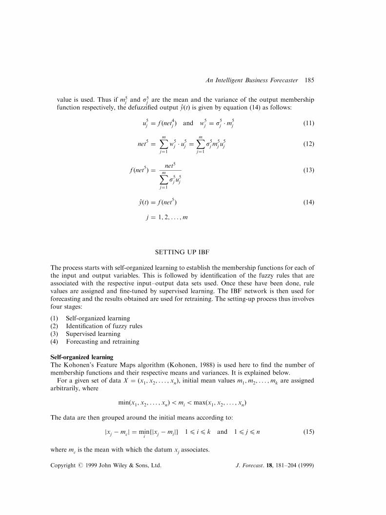
value is used. Thus if m5j and s5j are the mean and the variance of the output membership

function respectively, the defuzzi®ed output y�t� is given by equation (14) as follows:

u5j � f �net4j � and w

5j � s5j �m5

j �11�

net5 �

Xmj�1

w5j � u5j �

Xmj�1

s5j m5j u

5j �12�

f �net5� � net5Xmj�1

s5j u5j

�13�

y�t� � f �net5� �14�

j � 1; 2; . . . ;m

SETTING UP IBF

The process starts with self-organized learning to establish the membership functions for each ofthe input and output variables. This is followed by identi®cation of the fuzzy rules that areassociated with the respective input±output data sets used. Once these have been done, rulevalues are assigned and ®ne-tuned by supervised learning. The IBF network is then used forforecasting and the results obtained are used for retraining. The setting-up process thus involvesfour stages:

(1) Self-organized learning(2) Identi®cation of fuzzy rules(3) Supervised learning(4) Forecasting and retraining

Self-organized learningThe Kohonen's Feature Maps algorithm (Kohonen, 1988) is used here to ®nd the number ofmembership functions and their respective means and variances. It is explained below.

For a given set of data X � �x1; x2; . . . ; xn�, initial mean values m1;m2; . . . ;mk are assignedarbitrarily, where

min�x1; x2; . . . ; xn�5mi 5max�x1; x2; . . . ; xn�

The data are then grouped around the initial means according to:

jxj ÿ mcj � minifjxj ÿ mijg 14 i4 k and 14 j4 n �15�

where mc is the mean with which the datum xj associates.



Data groupings and the mean values are optimized by the following iterative process. Let xj�t�be an input and mc�t� the value of mc at iteration t (t � 0, 1, 2, . . . ), then

mc�t � 1� � mc�t� � a�t��xj�t� ÿ mc�t�� 16�

if xj belongs to the grouping of mc, and

mc�t � 1� � mc�t� �17�

if xj does not belong to the grouping of mc.Note that a�t� �05 a�t�5 1� is a monotonically decreasing scalar learning rate. The iteration

stops at a certain number of cycles decided by the user or when the condition jmc�t � 1� ÿmc�t�j4d is satis®ed, where d is an error limit assigned by the user. The variances of membershipfunctions can be determined by

si �1

R

��1

pi

Xpij�1�xj ÿ mi�2

vuut �14 i4 k� �18�

where

si � variance of membership function imi � mean of membership function ixj � observed data samplek � total number of membership function nodespi � total number of data samples in ith membership function groupR � overlap parameter.

For a given input or output variable, the number of initial mean values �m1;m2; . . . ;mk�is assigned by trial and error. This involves striking a balance between learning time andaccuracy. Too small a number results in an oversimpli®ed structure and might therefore adverselya�ect accuracy. On the other hand, too large a number increases network complexityunnecessarily, resulting in a considerable increase in learning time with very little or no increasein accuracy.

Identi®cation of fuzzy rulesAfter the membership functions have been constructed, the next stage is to identify the fuzzyrules using the same sets of data samples. The identi®cation process starts with a fully con-nected neural network structure. The total number of initial rules is bounded above by T�x1� �T�x2� � . . . �T�xk� � . . . � T�xp�, where T�xk� is the number of membership functions of the kthinput variable.

A set of input data are fed into the network from layer 1 and are fuzzi®ed in layer 2. Afuzzy AND operation is performed on the fuzzi®ed data in layer 3, followed by a fuzzy ORoperation in layer 4. The fuzzy IF±AND±THEN rule associated with this particular set ofinput data is represented by the links connecting the winner node of the min±max operationin layer 3 and the relevant nodes in layer 2. This rule-identi®cation process is illustrated inFigure 3.



Supervised learningThe objective of supervised learning is to minimize the error function E as de®ned byequation (19) below, by ®ne-tuning the rule values �rij�:

E � 12�y�t� ÿ y�t��2 �19�

where y(t) is the actual output and y�t� the predicted output.From the Backpropagation algorithm of Rumelhart [1986], we have:

w�t � 1� � w�t� ÿ Z@E

@w�20�

where w is any adjustable parameter in a given node, and Z is the assigned learning rate.Thus, the rule values (rij) can be ®ne-tuned as follows:

rij�t � 1� � rij�t� ÿ Z@E

@rij�21�

where@E

@rij� @E

@f �net4j �� @f �net

4j �

@�net4j �� @�net

4j �

@rij�22�

From equations (10)±(14) we have:

@E

@f �net4j �� @E

@u5j� @E

@f �net5� �@f �net5�@u5j

�23�

@E

@f �net5� �@E

@y�t� �@f1=2�y�t� ÿ y�t��2g

@y�t� � ÿ�y�t� ÿ y�t�� 24�

@f �net5�@u5j

� �Ss5j �m5

j � u5j � � s5j �m5j ÿ �Ss5j �m5

j � u5j � � s5jSs5j � u5j

�25�

@f �net4j �@�net4j �

� 1 �26�

@�net4j �@rij

� u4cj �27�

Figure 3. Fuzzy rule identi®cation process



From equations (20)±(26) we have

rij�t � 1� � rij�t� � Zu4cj�y�t� ÿ y�t��

Xmj�1

s5j u5j

!s5j m

5j ÿ

Xmj�1

s5j m5j u

5j

!s5j

Xmj�1

s5j u5j

!2�28�

where

rij�t� � rule weight (or rule value) associated with the rule represented by the link connectingnode i in layer 3 to node j in layer 4 at time period t

u4ij � input to node j in layer 4 from node i in layer 3Z � learning rate

y(t) � actual outputy�t� � predicted outputm5

j � mean of output membership function j in layer 5s5j � variance of output membership function j in layer 5u5j � input to node j in layer 5.

The learning process is iterated until an acceptable error between actual output y(t) andpredicted output y�t� is achieved. The rules identi®ed in stage 3 and their associated rules valuesare then stored in a rule base.

Forecasting and retrainingOnce the membership functions have been constructed, the fuzzy rules identi®ed and the initialrule values assigned and ®ne-tuned, the IBF network is ready for forecasting. For a given inputdata set, if the fuzzy rule identi®ed during forecasting does not match any of the existing rules inthe rule base, the system will choose* as replacement from the rule base a rule that is closest{ tothe rule identi®ed, and will then proceed to forecasting as usual. This will unavoidably introduceerrors into the forecasting result. It is therefore important that a large enough pool of datasamples be used to ensure that the training is complete.

The IBF network can be retrained whenever new data become available. Retraining involvesrepeating stages 1 to 3 to reconstruct membership functions, identify new fuzzy rules, if any, andupdate rule values. In general, the more the IBF network is used, the more data samples will beavailable for retraining. And the more it is retrained, the more accurate it will be.

ILLUSTRATIVE EXAMPLES

The IBF architecture has been implemented in a computer software using Microsoft VisualBasic in Windows 95. The IBF software tool has been applied to several real cases. Two suchcases are presented in the following sections. In both cases, the learning time includes (1) thecomputational time of Kohonen's Feature Maps algorithm and the competitive learning law,and (2) the convergence time of the Backpropagation Learning algorithm.

* In the event of a tie, i.e. two or more possible replacements exist, one is selected at random.{ The closeness between two rules is measured in terms of the number of common membership function nodes that therules involve.



Case IThe ®rst case is the forecasting of the US dollar to Singapore dollar exchange rate. Three inputvariables which were thought to have an in¯uence over the exchange rate were selected. They wereStock Exchange of Singapore Indices (x1), Domestic Interest Rates (x2), and Exports Value (x3).The selection was based on the ®ndings of research work in the Business School of NanyangTechnological University (Cheung, 1997; Yip, 1994). Results of an econometric analysis carriedout by the authors to analyse the relationships between the three variables and the exchange ratealso supported the selection (see Appendix A). Data used for training and testing were obtainedfrom statistical reports (Yearbook of Statistics 1990±1995) published by the Department ofStatistics, Singapore. A total of 69 data sets as listed in Table I were obtained, of which the ®rst50 samples ( from 01/1990 to 02/1994) were usedd for training and the rest for testing.

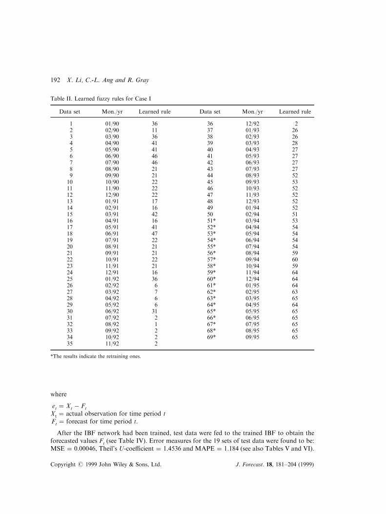
The data samples were ®rst normalized to the range of {0, 1}. The number of membershipfunction nodes was set for each input variable after studying the distribution patterns of the datasamples. There were three nodes (low, medium, high) for x1 , ®ve (very low, low, medium, high,very high) for x2 , ®ve (very low, low, medium, high, very high) for x3 , and three (low, medium,high) for y. Therefore, the maximum number of possible fuzzy rules was 75, which is 3� 5� 5.Membership functions were constructed for each variable. Figure 4 shows the membershipfunctions of x1 before and after learning with an overlap parameter of 0.4. Table II gives thelearned fuzzy rules and the data sets they each associate. Table III shows the learned rules, and theinitial and learned rule values. Figure 5 summarizes the learning performance in terms of MeanSquare Error (see below) as a function of number of epochs with an assigned learning rate of 0.5.

Figure 4. Membership function of x1 before and after learning for Case I

Figure 5. MSE versus time (epochs) for Case I



Table I. Data sets for IBF training and testing for Case I

No. Mon./yr ER(S$/per US$)

(Y)

SES(million S$)

(X1)

DIR(%/yr)(X2)

EV(million S$)

(X3)

1 01/90 1.8895 423.4 6.28 7235.72 02/90 1.8637 435.9 6.60 6573.33 03/90 1.8774 431.1 6.65 8573.64 04/90 1.8775 415.5 7.03 7010.05 05/90 1.8570 426.6 7.23 7750.86 06/90 1.8463 433.8 7.60 7615.47 07/90 1.8200 440.5 7.65 7628.68 08/90 1.7910 373.8 7.90 7999.19 09/90 1.7654 336.6 7.90 7978.410 10/90 1.7267 316.0 7.90 9266.111 11/90 1.7084 311.1 7.88 8733.412 12/90 1.7265 322.6 7.73 8841.613 01/91 1.7454 326.9 7.45 9241.114 02/91 1.7176 348.7 7.43 7201.915 03/91 1.7565 408.7 7.43 8855.016 04/91 1.7693 392.3 7.43 8352.217 05/91 1.7679 413.9 7.43 8309.318 06/91 1.7780 412.4 7.71 8894.219 07/91 1.7566 398.6 7.91 9102.120 08/91 1.7269 383.6 7.91 8492.021 09/91 1.7019 382.8 7.85 8469.922 10/91 1.6928 379.1 7.70 8813.523 11/91 1.6716 396.3 7.65 8255.324 12/91 1.6461 393.0 7.10 7893.025 01/92 1.6332 411.4 6.55 8190.326 02/92 1.6366 405.5 6.18 6954.227 03/92 1.6596 388.6 6.18 8746.428 04/92 1.6564 380.6 6.18 7853.029 05/92 1.6399 397.3 6.18 8047.130 06/92 1.6239 405.0 6.13 8746.432 08/92 1.6076 369.2 5.86 8370.233 09/92 1.5983 364.6 5.63 9105.834 10/92 1.6064 358.0 5.55 9008.835 11/92 1.6323 374.9 5.55 9101.836 12/92 1.6394 384.1 5.55 10137.437 01/93 1.6531 401.0 5.55 8023.338 02/93 1.6468 413.4 5.55 8504.739 03/93 1.6446 418.1 5.38 10457.940 04/93 1.6229 432.5 5.36 10291.741 05/93 1.6131 455.7 5.36 9656.542 06/93 1.6164 456.5 5.36 9972.843 07/93 1.6211 451.3 5.36 10423.244 08/93 1.6098 489.0 5.36 9712.845 09/93 1.5973 514.8 5.36 11307.046 10/93 1.5716 545.1 5.34 9942.747 11/93 1.5951 547.6 5.34 10437.948 12/93 1.5977 595.2 5.34 10742.8

Table continued over page



Error measures for forecasting accuracy have attracted much attention over the past few years.Many studies have been carried out to investigate their suitability for measuring the accuracy offorecasting methods (Armstrong and Collopy, 1992; Fildes, 1992). However, results seem toindicate that no single accuracy measure can capture all the nuances of a forecasting method orthe relative merits of di�erent forecasting methods. In view of this, forecasting errors in this studywere examined with three commonly used error measures, namely: Mean Squared Error (MSE),Theil'sU-coe�cient (U) andMean Absolute Percentage Error (MAPE) (Makrodakis et al., 1982,1983; Thompson, 1990; Collopy and Armstrong, 1992; Ahlburg et al., 1992). For n error terms,they can be expressed as:

MSE �Xni

e2i =n �29�

Theil0s U coefficient �

��Xnÿ1i�1

Fi�1 ÿ Xi�1Xi

� �2

Xnÿ1i�1

Xi�1 ÿ Xi

Xi

� �2

vuuuuuuut �30�

MAPE �Xnt�1

jXt ÿ FtjXt

�100�=n �31�

Table I. Continued

No. Mon./yr ER(S$/per US$)

(Y)

SES(million S$)

(X1)

DIR(%/yr)(X2)

EV(million S$)

(X3)

49 01/94 1.6032 607.9 5.50 10329.650 02/94 1.5879 605.9 5.59 8532.451 03/94 1.5819 560.2 5.59 11439.452 04/94 1.5622 557.4 5.66 12259.653 05/94 1.5463 570.0 5.73 12321.954 06/94 1.5304 556.2 5.73 13220.755 07/94 1.5144 546.5 5.73 12461.546 08/94 1.5043 568.9 6.01 13324.657 09/94 1.4891 571.4 6.01 13659.458 10/94 1.4763 579.4 6.01 13204.759 11/94 1.4681 560.9 6.49 13289.460 12/94 1.4651 526.3 6.49 13294.961 01/95 1.4523 509.1 6.49 12311.762 02/95 1.4538 511.4 6.49 11562.063 03/95 1.4203 502.9 6.49 14137.564 04/95 1.3985 497.6 6.49 12650.565 05/95 1.3937 518.9 6.49 13778.566 06/95 1.3949 519.1 6.34 14407.367 07/95 1.3984 521.2 6.34 14100.368 08/95 1.4125 509.2 6.26 14958.369 09/95 1.4341 513.7 6.26 14883.2

Source: Singapore Statistical Board 1990±1995



where

et � Xt ÿ Ft

Xt � actual observation for time period tFt � forecast for time period t.

After the IBF network had been trained, test data were fed to the trained IBF to obtain theforecasted values Ft (see Table IV). Error measures for the 19 sets of test data were found to be:MSE � 0.00046, Theil's U-coe�cient � 1.4536 and MAPE � 1.184 (see also Tables V and VI).

Table II. Learned fuzzy rules for Case I

Data set Mon./yr Learned rule Data set Mon./yr Learned rule

1 01/90 36 36 12/92 22 02/90 11 37 01/93 263 03/90 36 38 02/93 264 04/90 41 39 03/93 285 05/90 41 40 04/93 276 06/90 46 41 05/93 277 07/90 46 42 06/93 278 08/90 21 43 07/93 279 09/90 21 44 08/93 5210 10/90 22 45 09/93 5311 11/90 22 46 10/93 5212 12/90 22 47 11/93 5213 01/91 17 48 12/93 5214 02/91 16 49 01/94 5215 03/91 42 50 02/94 5116 04/91 16 51* 03/94 5317 05/91 41 52* 04/94 5418 06/91 47 53* 05/94 5419 07/91 22 54* 06/94 5420 08/91 21 55* 07/94 5421 09/91 21 56* 08/94 5922 10/91 22 57* 09/94 6023 11/91 21 58* 10/94 5924 12/91 16 59* 11/94 6425 01/92 36 60* 12/94 6426 02/92 6 61* 01/95 6427 03/92 7 62* 02/95 6328 04/92 6 63* 03/95 6529 05/92 6 64* 04/95 6430 06/92 31 65* 05/95 6531 07/92 2 66* 06/95 6532 08/92 1 67* 07/95 6533 09/92 2 68* 08/95 6534 10/92 2 69* 09/95 6535 11/92 2

*The results indicate the retraining ones.



Case IIThe second case is the forecasting of electricity consumption of Singapore. Here the inputlinguistic variables selected were the same as those used by Liu et al. (1991) in a similar study.They were Gross Domestic Product (x1), Price Index of Electricity (x2) (output variable of ISG)and Population of Singapore (x3). Results of an econometric analysis performed by Liu et al.(1991) of the relationships between the three variables and the output variable (y), i.e. theelectricity consumption, supported the selection (see Appendix B). A total of 37 data sampleswere used (see Table VII). Of which, the ®rst 25 samples ( from 1960 to 1984) were used fortraining, and the rest for testing.

Table III. Initial and learned rule values for Case I

Rule IF-AND preconditions THEN post-conditions

Input (X) Output (Y)

X1 X2 X3 Initial rule value (rij) Learned rule value (rij)

Low( j � 1)

Medium( j � 2)

High( j � 3)

Low( j � 1)

Medium( j � 2)

High( j � 3)

1 L VL VL 0.7055 0.5334 0.5795 0.8145 0.5231 0.43042 L VL L 0.2896 0.3019 0.7747 0.8271 0.4335 0.56736 L L VL 0.9620 0.8714 0.0562 0.6643 0.9608 0.64007 L L L 0.9496 0.3640 0.5249 0.7026 0.3764 0.830611 L M VL 0.8293 0.8246 0.5892 ÿ0.4426 0.5640 1.226916 L H VL 0.1001 0.1030 0.7989 0.5562 0.4795 1.388517 L H L 0.2845 0.0456 0.2958 0.1208 0.0806 0.575821 L VH VL 0.4101 0.4128 0.7127 0.3882 0.6735 1.490522 L VH L 0.3262 0.6332 0.2076 0.1733 0.8398 0.972226 M VL VL 0.9194 0.6316 0.6276 0.7726 0.6365 0.802027 M VL L 0.4285 0.0980 0.5610 0.6175 0.1202 0.418528 M VL M 0.6945 0.9137 0.8348 0.7802 0.9173 0.751531 M L VL 0.5137 0.4630 0.3535 0.5161 0.4628 0.350336 M M VL 0.6288 0.5421 0.1563 ÿ0.2052 1.1323 2.774842 M H L 0.1282 0.0002 0.5368 0.1088 ÿ0.0045 0.544346 M VH VL 0.7044 0.9288 0.5302 ÿ0.3891 0.7737 1.277547 M VH L 0.0896 0.7577 0.4018 ÿ0.1831 0.6963 0.522451 H VL VL 0.4439 0.2729 0.8725 0.9302 0.2888 0.386552 H VL L 0.7507 0.2729 0.6736 1.0127 0.3071 0.486053 H VL M 0.2566 0.0899 0.3010 0.5930 0.2859 0.229754 H VL H 0.3227 0.7901 0.2973 1.0431 0.9367 ÿ0.066759 H L H 0.5429 0.0807 0.6344 0.9294 0.0008 0.019360 H L VH 0.4100 0.9604 0.1146 0.5710 0.8845 ÿ0.280863 H M M 0.9937 0.1304 0.0289 1.0062 0.1007 ÿ0.070764 H M H 0.3454 0.5477 0.9230 2.0645 0.7115 0.483265 H M VH 0.5382 0.4064 0.8472 2.0205 0.5211 0.4420

VLÐinput membership term of `Very Low'.MÐinput membership term of `Medium'.VHÐinput membership term of `Very High'.LÐinput membership term of `Low'.HÐinput membership term of `High'.



Table IV. IBF test results for Case I

Data set Mon./yr Actual YA Forecast YB

51 03/94 1.5819 1.597352 04/94 1.5622 1.588053 05/94 1.5463 1.566954 06/94 1.5304 1.551555 07/94 1.5144 1.533456 08/94 1.5043 1.530957 09/94 1.4891 1.504058 10/94 1.4763 1.504059 11/94 1.4681 1.484760 12/94 1.4651 1.469361 01/95 1.4523 1.465362 02/95 1.4538 1.452363 03/95 1.4203 1.452364 04/95 1.3985 1.452365 05/95 1.3937 1.428166 06/95 1.3949 1.398467 07/95 1.3984 1.396368 08/95 1.4125 1.397969 09/95 1.4341 1.4088

Error measures MSE 0.00046U-coe�cient 1.4536MAPE 1.1840

Table V. Performance of di�erent BPN structures for Case I

Network structure BPN A BPN B BPN C

Layers Input Hidden Output Input Hidden Output Input Hidden Output

Number of layers 1 3 9 1 3 1 3 9 1 1 9 3 1Number of nodes 3 9 27 3 3 3 9 27 3 3 27 9 3MSE 2.983� 10ÿ4 2.941� 10ÿ3 2.866� 10ÿ3Accuracya 97.81% 97.72% 97.76%

Number of epochs � 25,000; learning rate � 0.5; learning momentum � 0.4.a The percentage average of calculated values over actual ones.

Table VI. Forecasting accuracy of BPN for di�erent numbers of epochs for Case I

Network structure(BPN A)

1 input layer � 3 hidden layers � 1 output layer

No. of epochs 25000 10000 5000 2500 1000 800 500 100

MSE 2.941� 10ÿ3

2.945� 10ÿ3

3.244� 10ÿ3

3.400� 10ÿ3

4.205� 10ÿ3

5.413� 10ÿ3

7.536� 10ÿ3

8.035� 10ÿ3

Accuracy 97.81% 97.77% 97.63% 97.54% 97.26% 96.72% 95.62% 95.56%



The data samples were also normalized to the range of {0, 1}. Again, the number of member-ship function nodes was set for each of the input and output variables after studying the distri-bution patterns of the data samples. There were three nodes (low, medium, high) for each of x1 ,x2 , x3 and y. Here the total number of fuzzy rules was bounded above by 3� 3� 3 � 27. Figure 6shows the membership functions of x1 before and after learning with an overlap parameter of 0.4.Table VIII shows the learned fuzzy rules and the data sets they each associate. Figure 7

Table VII. Data sets for IBF training and testing for Case II

Data set Year X1 X2 X3 Y

1 1960 2149.60 51.43 1646.40 589.702 1961 2329.10 51.33 1702.40 638.903 1962 2513.70 50.83 1750.20 689.604 1963 2789.90 50.34 1795.00 729.905 1964 2714.60 52.12 1841.60 828.006 1965 2956.20 53.71 1886.90 912.507 1966 3330.70 54.20 1934.40 1074.908 1967 3745.70 56.78 1977.60 1238.609 1968 4315.00 57.38 2012.00 1446.8010 1969 5019.90 59.56 2042.50 1652.9011 1970 5804.90 60.84 2074.50 1941.6012 1971 6823.30 61.74 2112.90 2268.9013 1972 8155.80 62.13 2152.40 2776.8014 1973 10205.10 65.50 2193.00 3304.3015 1974 12543.20 83.44 2229.80 3426.2016 1975 13373.00 87.00 2262.60 3673.3017 1976 14575.20 96.02 2293.30 4038.0018 1977 15968.90 97.51 2325.30 4506.4019 1978 17750.60 98.10 2353.60 5213.7020 1979 20452.30 108.21 2383.50 5743.7021 1980 24200.50 139.33 2413.90 6198.0022 1981 28369.00 146.36 2443.30 6660.4023 1982 31348.40 150.10 2471.80 7000.1024 1983 36732.80 142.40 2502.00 7697.6025 1984 40047.90 139.20 2529.10 8398.8026 1985 38923.50 138.20 2558.00 8871.2027 1986 38663.50 122.10 2586.20 9475.8028 1987 42635.80 110.90 2612.80 10616.6029 1988 49998.00 108.30 2647.10 11734.8030 1989 56844.20 102.40 2647.60 12687.5031 1990 63438.90 108.30 2705.10 14194.4032 1991 69451.70 107.10 2762.70 15088.9033 1992 74974.50 98.40 2818.20 15948.0034 1993 85473.20 100.20 2873.80 17194.1035 1994 94063.60 98.30 2930.20 18901.3036 1995 102299.10 101.50 2986.50 20239.5037 1996 108756.80 105.30 3044.30 23668.90

X1ÐGross domestic product (million S$).X2ÐPrice index of electricity (1993 � 100).X3ÐPopulation of Singapore (thousands).YÐElectricity consumption (million kWh).



summarizes the learning performance in terms of MSE as a function of number of epochs with anassigned learning rate of 0.5. Twelve sets of test data were fed to the trained IBF to obtain theforecasted values YB (see Table IX). Forecasting accuracy for the three error measures werefound to be: MSE � 2.6� 106, Theil's U-coe�cient � 1.0988 and MAPE � 8.5792.

COMPARISON WITH CONVENTIONAL NEURAL NETWORKS

A study has also been made of the performance of IBF in comparison with that of twoconventional nerual networks basing on the two cases in the previous section. The twoconventional neural networks involved are Back-propagation Network (BPN) and Radial-basisFunction Network (RBFN). BPN is a multi-layered feedforward network in which functionapproximation is achieved by means of gradient descent optimization using backpropagation(Lippmann, 1987; Rumelhart et al., 1986; Haykin, 1994). RBFN is a network which makes use ofradially symmetric transfer functions in its hidden layer to achieve function approximation(Poggio and Girosi, 1990; Broomhead and Lowe, 1989; Moody and Darken, 1989; Leonard et al.,1991, 1992; Renals, 1989).

Figure 6. Membership function of x1 before and after self-learning for Case II

Figure 7. MSE versus time (epochs) for Case II



Both the BPN and RBFN models used in the study were developed using the commercialsoftware package `NeuralWorks Version 5' (NeuralWare Inc., 1993). The parameters of bothmodels included number of layers, number of nodes of each layer, number of epochs tostabilization, learning rates, and momentum values. They were set more or less by trial and errorin this study to give the `best' possible performance. The details are given in Appendix C. In both

Table VIII. Learned fuzzy rules for Case II

Data set Year Learned rule Data set Year Learned rule

1 1960 1 21 1980 82 1961 1 22 1981 83 1962 1 23 1982 84 1963 1 24 1983 175 1964 1 25 1984 176 1965 1 26a 1985 177 1966 1 27a 1986 178 1967 1 28a 1987 149 1968 1 29a 1988 1410 1969 1 30a 1989 1411 1970 1 31a 1990 1412 1971 1 32a 1991 1513 1972 1 33a 1992 2414 1973 1 34a 1993 2416 1975 4 36a 1995 2417 1976 4 37a 1996 2418 1977 5 38b 1997 2419 1978 5 39b 1998 2720 1989 5 40b 1999 27

aResults for retraining.bResults for forecasting.

Table IX. IBF test results for Case II

Data set Year Actual YA Forecast YB

26 1985 8871.20 8321.8927 1986 9475.80 8783.1528 1987 10616.60 9354.2229 1988 11734.80 10617.3730 1989 12687.50 11611.5131 1990 14194.40 12520.0432 1991 15088.90 13908.8833 1992 15948.00 15088.2934 1993 17194.10 15946.9835 1994 18901.30 17055.0736 1995 20239.50 18623.3437 1996 23668.90 19944.83

Error measures MSE 2.6� 106

Theil's U 1.0988MAPE 8.5792



cases, the BPN model used comprised ®ve layers: one input layer, three hidden layers and oneoutput layer; while the RBFN model comprised three layers: one input, one prototype and oneoutput layer. The learning rules and transfer functions used for BPN were Delta and Sigmoid,respectively; while they were Norm-Cum-Delta and Gaussian for RBFN. Table X summarizesthe parametric set-ups of both models.

Figures 8 and 9 compare the forecasted values of IBF and BPNwith the actual values for Case Iand Case II respectively, while Figures 10 and 11 compare that of IBF and RBFN with the actualvalues for the same two cases. Table XI compares the learning performance of IBF with that ofBPN andRBFN for the two cases, while Table XII compares their forecasting performances. The

Table X. Parametric set-ups of the BPN and RBFN models

Neuralnetworkmodel

Learningrates

Momentum* Learningrule

Transferfunction

No. of layers and no. of nodes in each layer

Inputlayer

Hiddenlayer 1

Hiddenlayer 2

Hiddenlayer 3

Outputlayer

BPN 0.5 0.4 Deltaa Sigmoid 3 9 27 3 1

Inputlayer

Prototype layer Outputlayer

RBFN 0.5 0.4 Norm-cum-delta*

Gaussian 3 50 1

a See NeuralWare Inc. (1994).

Table XI. Learning performance of IBF, BPN and RBFN

Neural network model Learning epochs Learning rate MSE Time taken (minutes)

Case I IBF 50 10.0 0.00001 0.30a

BPN 10000 0.5 0.00265 5.00b

RBFN 10000 0.5 0.00171 2.00b

Case II IBF 420 5.0 4.06� 102 0.15a

BPN 10000 0.5 4.87� 105 4.00b

RBFN 10000 0.5 1.51� 104 1.50b

a System set-up after each iteration is automatic.bDoes not include system set-up time after each iteration.

Table XII. Forecasting performance of IBF, BPN and RBFN

Neural network model MSE Theil's U MAPE (%)

Case I IBF 0.00046 1.4536 1.1840BPN 0.07058 11.9768 14.5311RBFN 0.07279 12.2005 14.7841

Case II IBF 2.6� 106 1.0988 8.5792BPN 1.76� 108 1.6472 13.9341RBFN 3.43� 107 4.6379 37.3806



number of epochs in Table X indicates the point where learning convergence starts to stabilize.The networks were retrained after every prediction, using the latest input±output data sets.Figures 5 and 7 show that the learning curves for IBF are rather steep converging rapidly to anMSE of about 0.00001 and 4.06� 102 for Case I and Case II respectively.

Figure 8. US dollar to Singapore dollar exchange rate, actual and forecasted by IBF and BPN

Figure 9. US dollar to Singapore dollar exchange rate, actual and forecasted by IBF and RBFN

Figure 10. Electricity consumption, actual and forecasted by IBF and BPN



Results in Table XII show that IBF is at least eight times as accurate compared with BPN andRBFN in terms of the three error measures for both cases. Results in Table XI show that IBFlearns at least ®ve times as fast: IBF needs only 50 epochs taking about 18 seconds to learn theinput data patterns for Case I on an IBM Pentium 166 MHz compatible, and 20 epochs takingabout 10 seconds for Case II; while both BPN and RBFN need about 10,000 epochs taking atleast 90 seconds.

The superior performance of IBF may be attributed to the e�ectiveness of the algorithm forself-learned fuzzy rules. Although a large number of rule nodes may exist in the rule layer of IBF,only one rule is involved at a time for each data set. This means that both learning and forecastingof IBF follow a speci®c path through the network, rather than involving all the nodes andconnections as in the case of the traditional neural networks. This greatly reduces the complexityof the network structure, speeds up the learning and forecasting processes, and increasesforecasting accuracy. Such superior performance of the fuzzy-neural network hybrid systemsover the pure neural network systems is not uncommon in other application areas like processcontrol (Lin and Lee, 1992) and image processing (Adeli and Hung, 1995).

The IBF model is able to automatically update its membership functions as well as its fuzzyrules and rule values after every run, using the latest input±output data sets that are availableon-line. It therefore also has the capability to update the forecasting trend dynamically as theexternal environment changes over time.

CONCLUSIONS

The architectural design of an intelligent business forecaster has been presented. The intelligentforecaster, which is basically a ®ve-layer fuzzy rule-based neural network, has been used toforecast the Singapore dollar to the US dollar exchange rate, and the electricity consumption ofSingapore. Its performance has been compared with that of Backpropagation Neural Networksand Radial-basis Function Neural Networks. The results show that the intelligent forecaster issuperior to the other two in terms of both learning speed and forecasting accuracy. Comparedwith pure neural network systems, the fuzzy logic-neural network hybrid system as proposed inthis paper thus seems to be able to provide a better solution to the problems of businessforecasting in today's environment.

Figure 11. Electricity consumption, actual and forecasted by IBF and RBFN



APPENDIX A: ECONOMETRIC ANALYSIS OF THE SINGAPORE DOLLAR TO USDOLLAR EXCHANGE RATE

An econometric model of the Singapore dollar to the US dollar exchange rate was developed bythe authors using the commercial software package `Statistical Analysis System' (SAS InstituteInc., 1990). The model is as follows:

Y � 1.3045 � 0.0945 ln�X1� � 0.0386�X2� ÿ 0.00005�X3�T � �3.302� �1.484� �3.905� �ÿ11.074�R

2 � 0.8; F � 84.625

where

X1 � stock exchange of Singapore indicesX2 � domestic interest ratesX3 � exports valueY � real exchange rate of Singapore dollar to US dollar.

The function form was selected by trial and error. The coe�cients were estimated using theordinary least squares method and examined with a t-test. Regression shows that x1 and x2 havepositive correlation with y, while x3 has negative. The ®gures in parentheses are the t-test valuesof the corresponding coe�cients under which the ®gures are located. The individual coe�cientsare statistically signi®cant at the 95% con®dent level. The F-test indicates that the in¯uence of theinput variables on the output is signi®cant. The R2-test con®rms that the calculated values usingthe equation agree well with the actual values.

APPENDIX B: ECONOMETRIC ANALYSIS OF ELECTRICITY CONSUMPTIONOF SINGAPORE

The econometric model as developed by Liu et al. (1991) for the analysis of Singapore's electricityconsumption is as follows:

ln�Y� � ÿ0.39 � 0.309 ln�X1� ÿ 0.162 ln�X2� � 1.001 ln�X3� � 0.64 ln�Yÿ1�T � �5.76� �0.33� �1.35� �0.0�R

2 � 0.999; D±W � ÿ1.587; MSE � 0.0074

where

X1 � gross domestic productX2 � price index of electricityX3 � population of SingaporeY � electricity consumption

The ®gures in parentheses are the t-test values of the corresponding coe�cients under whichthe ®gures are located. All the coe�cients give the right signs. They are all statistically signi®cant



at the 95% con®dent level, except for ln(X1) which is only marginally lower. The R2-value is closeto 1 indicating a very good ®t. The D±W test shows that there is no serial correlation among thedisturbances.

APPENDIX C: PARAMETRIC SET-UP OF BPN AND RBFN

The parameters of both the BPN and RBFN models include number of layers, number of nodesof each layer, number of epochs to stabilization, learning rates, and momentum values. In thisstudy, they were set more or less by trial and error to give the `best' possible performance in termsof learning speed and forecasting accuracy.

(1) Learning ratesDi�erent learning rates were tested with both models using a momentum value of 0.4 (see (2)below). For RBFN, additional tests were carried with three di�erent network structures (see (3)below). A learning rate of 0.5 was found to be the `best' for both BPN and RBFN, and was usedthroughout the study. Too small a learning rate will result in the network taking an unnecessarilylong time to stabilize, while too large a rate will destabilize the network.

(2) Momentum valuesThe default value of 0.4 was used throughout the study. It was found that changes in momentumvalue (within the range of 0 and 1) had very little or no e�ect on the performance of both models.

(3) Number of layers and number of nodes of each layerFor RBFN, the number of layers and the number of nodes of each layer are ®xed and cannot bealtered. For BPN, three di�erent feasible network structures were tested: the ®rst structure hasthree hidden layers 9 � 27 � 3 (the ®rst hidden layer has nine nodes, the second has 27 nodes, andthe third has three nodes); the second structure has two hidden layers 9 � 27; the third also hastwo hidden layers 27 � 9. Results in Table V show that the three structures have more or less thesame performance in terms of both MSE and average accuracy. The ®rst structure was chosenarbitrarily and used throughout the study.

(4) Number of epochsThe selected network structures for both BPN and RBFN were run for di�erent numbers ofepochs. Table VI summarizes the results for BPN. As can be seen from the table, MSE remainsfairly constant when the epoch number is 10,000 and above. In this study, the number of epochswas set at 25,000 throughout for both models. Similar results were obtained for RBFN.

REFERENCES

Adeli, H. and Hung, S. L.,Machine Learning: Neural Networks, Genetic Algorithm and Fuzzy Systems, NewYork: John Wiley, 1995.

Ahlburg, D. A. et al. `A commentary on error measures', International Journal of Forecasting, 8 (1992).Armstrong, J. S. and Collopy, F., `Error measures for generalizing about forecasting methods: Empiricalcomparisons', International Journal of Forecasting, 8 (1992).



Azo�, E. M., Neural Network Time Series Forecasting of Financial Markets, New York: John Wiley, 1994.Broomhead, D. S. and Lowe, D., `Multivariable functional interpolation and adaptive networks', RSREMemorandum No. 4341, Royal Signals and Radar Establishment, Malvern, UK, 1989.

Cheung, Y. W. and Chinn, M. D., Ìntegration, cointegration and the forecast consistency of structuralexchange rate models', Working Paper Series 5943, National Bureau of Economic Research, 1997.

Cho, S. B., À neural-fuzzy architecture for high performance classi®cation', in Furuhashi, T. (ed.),Advances in Fuzzy Logic, Neural Networks and Genetic Algorithms, New York: Springer-Verlag, 1991.

Collopy, F. and Armstrong, J. S., `Rule-based forecasting: Development and validation of an expertsystems approach to combining time series extrapolations', Management Science.

Department of Statistics, Yearbook of Statistics, Singapore, 1990±1995.Fildes, R., `The evaluation of extrapolative forecasting methods', International Journal of Forecasting, 8(1992).

Foslien, W. and Samad, T., `Fuzzy controllers synthesis with neural network process models', inGoonatilake, S. and Khebbal, S. (eds), Intelligent Hybrid Systems, New York: John Wiley, 1995.

Haykin, S., Neural Networks: A Comprehensive Foundation, New York: Macmillan College PublishingCompany, 1994.

Kang, S. Y., Àn Investigation of the Use of Feedforward Neural Networks for Forecasting', PhD thesis,Kent State University, 1991.

Kasahov, N. K., `Hybrid connectionist fuzzy systems for speech recognition and the use of connectionistproduction systems', in Furuhashi, T. (ed.), Advances in Fuzzy Logic, Neural Networks and GeneticAlgorithms, New York: Springer-Verlag, 1991.

Klimasauskas, C. C., Ùsing fuzzy pre-processing with neural networks for chemical process diagnosticproblems', in Goonatilake, S. and Khebbal, S. (eds), Intelligent Hybrid Systems, New York: John Wiley,1995.

Kohonen, T., Self-organization and Associative Memory, Berlin: Springer-Verlag, 1988.Kosko, B., Neural Networks and Fuzzy System, Englewood Cli�s, NJ: Prentice Hall, 1992.Leonard, J. A. and Kramer, M. A., `Radial basis functions for classifying process faults', IEEE ControlSystems, April (1991).

Leonard, J. A., Kramer, M. A. and Ungar, L. H., Ùsing radial basis functions to approximate a functionand its error bounds', IEEE Transactions on Neural Networks, 3 (1992).

Lippmann, R. P., Àn introduction to computing with neural nets', IEEE ASSP Magazine, 4 (1987), 4±22.Lin, C. T. and Lee, G. `Neural-network-based fuzzy logic control and decision system', IEEE Transactionson Computers, 40 (1992), No. 12, December.

Liu, X. Q., Ang, B. W. and Goh, T. N., `Forecasting of electricity consumption: a comparison between aneconometric model and a neural network model', Proceedings of IEEE International Joint Conference onNeural Networks, 1991.

Makridakis, S. et al. `The accuracy of extrapolation (time series) methods: Results of a forecastingcompetition', Journal of Forecasting, 1 (1982), 111±153.

Makridakis, S., Wheelwright, S. C. and Mcgee, V. E., Forecasting: Methods and Applications, 2nd edn, NewYork: John Wiley, 1983.

Moody, J. E. and Darken, C. J., `Fast learning in networks of locally-tuned processing units', NeuralComputation, 1 (1989).

NeuralWare Inc, NeuralWorks Professional II/Plus and NeuralWorks Explorer, 1993.Poggio, T. and Girosi, F., `Networks for approximation and learning', Proceedings of the IEEE (1990).Refenes, A.-P., Neural Networks in the Capital Markets, Chichester: John Wiley, 1995.Renals, S., `Radial basis function network for speech pattern classi®cation', Electronics Letters, 25 (1989).Rumelhart, D. E., Hinton, G. E. and Williams, R. J., `Learning internal representations by errorpropagation', Parallel Distributed Processing, Vol. 1, Cambridge: MIT Press, 1986.

SAS Institute Inc., Base SAS Software, Version 6, Cary, NC, USA: SAS Circle Box 8000, 1990.Taylor, J. G. and Mannion, C., Theory and Applications of Neural Networks, London: Springer Verlag,1992.

Thompson, P. A., Àn MSE statistic for comparing forecast accuracy across series', International Journal ofForecasting, 6 (1990).

Yip, P. S. L., Èxchange rate volatility and export performance in Singapore', Working Paper SeriesNo: 10-94, Nanyang Technological University, Singapore, 1994.



Zadeh, L. A., `Fuzzy sets', Information and Control, 8 (1965).Zurada, J. M., Introduction to Arti®cial Neural System, New York: West Publishing Company, 1992.

Authors' biographies:Xiang Li is currently a Research Engineer at Gintic Institute of Manufacturing Technology and a candidatefor the degree of PhD of Nanyang Technological University. Her current research interests include neuralnetworks, learning systems, fuzzy logic, statistical analysis, and decision support systems.

Cheng-Leong Ang is a Senior Research Fellow at the Gintic Institute of Manufacturing Technology. Hiscurrent research interests include enterprise engineering, design and analysis of manufacturing systems,IDEF modelling, and AI applications in manufacturing.

Robert Keng Leng Gay received his BEng, MEng, and PhD from the University of She�eld. He has manyyears of teaching and research experience in both Singapore and the United Kingdom. He joined NanyangTechnological University as an Associate Professor in 1982 and is now the Graduate Programme Director ofGintic Institute of Manufacturing Technology. His current research interests include AI applications,enterprise engineering, IDEF modelling, computer graphics, and factory automation. He is a CharteredEngineer and a Member of the Institution of Electrical Engineers, UK.

Authors' addresses:Xiang Li, Cheng-Leong Ang and Robert Keng Leng Gay, Gintic Institute of Manufacturing Technology,71 Nanyang Drive, Singapore 638075.



An intelligent business forecaster for strategic business planning

Documents

Transcript of An intelligent business forecaster for strategic business planning