An integrated processing scheme for high-resolution ...

An integrated processing scheme for high-resolutionairborne electromagnetic surveys, the SkyTEM system

Esben Auken1,5 Anders Vest Christiansen2 Joakim H. Westergaard3

Casper Kirkegaard1 Nikolaj Foged1 Andrea Viezzoli4

1The Hydrogeophysics Group, Department of Earth Sciences, University of Aarhus,Høegh-Guldbergs Gade 2, DK-8000 Aarhus C, Denmark.

2Geological Survey of Denmark and Greenland – GEUS, Department of Groundwater Mapping,Lyseng Alle 1, DK-8270, Højbjerg, Denmark.

3Orbicon A/S, Department of Water Resources and Applied Geophysics, Jens Juuls Vej 16,DK-8260, Viby J, Denmark.

4Aarhus Geophysics, Høegh-Guldbergs Gade 2, DK-8000 Aarhus C, Denmark.5Corresponding author. Email: [email protected]

Abstract. TheSkyTEMhelicopter-bornetransientelectromagneticsystemwasdevelopedin2004.Thesystemyieldsunbiaseddatafrom10to12msafter transmittercurrent turn-off.Thesystemisequippedwithseveraldevicesenablingacompletemodellingof the movement of the system in the air, facilitating excellent high-resolution images of the subsurface.

An integrated processing and inversion system for SkyTEM data is discussed. While the authors apply this system withSkyTEMdata, most of the techniques are applicable for airborne electromagnetic data in general. Altitude data are processedusinga simple recursivefiltering technique that efficiently removes reflections from trees.The technique is completely generaland can be used to filter altitude data from any airborne system. Raw voltage data that are influenced by electromagneticcoupling to man-made structures are culled from the dataset to avoid uncoupled data being distorted by coupled data,and geometrical corrections are applied to correct for pitch and roll of the transmitter frame. Data are de-spiked andaveraged using trapezoid-shaped filter kernels. A Laterally Constrained Inversion using smooth models is actively used toevaluate the processing, and the final inversion is tightly connected to the processing procedures.

Key words: airborne electromagnetic, altitude processing, constrained inversion, SkyTEM.

Introduction

Large airborne electromagnetic surveys are a logistical challenge,not only in carrying out the field operation, but also in thesubsequent data handling. The data handling can be dividedinto four steps: management, processing, inversion and, finally,presentation. These four steps involvemany different techniques,but common to all of them is a complicated logistic data flow.

The SkyTEM system is a relatively new helicopter-bornetransient electromagnetic system (Sørensen and Auken, 2004;Auken et al., 2007a). It was originally developed for high-resolution surveys targeting freshwater hydrological problems,but over the past few years it has been utilised in a wider rangeof applications including mapping buried iron ore palaeochannels(Reid and Viezzoli, 2007) and salinity (Viezzoli et al., 2007;Munday et al., 2007). On the Galapagos Islands the system gavehigh-resolution data forming the basis of a very comprehensivehydrological and geomorphological understanding of the SantaCruz Island (d’Ozouville et al., 2008). TheSkyTEMsystemdiffersfrom other systems in two ways. First, the system measures veryearly time data that are unbiased (unbiased means voltage datawhichatall timegateshavelessthan1%primaryresponse).Second,the geometry of the system is completely described and the entiremovement of the system in the air is at all times monitored.

In this paper we will discuss the implementation of the data-handling logistics for SkyTEM data. The implementation isbased on our background in hydrogeophysics, where minor

changes in data can change the outcome of the investigationfrom success to failure. Therefore, the need for not only high-precision unbiased data, but also high-quality processing, isinevitable. The processing entails using appropriate dataaveraging schemes, removing distorted data, and having accuratealtitude estimates. First, we will briefly present the SkyTEM setupand then, in greater detail, describe the data-handling system. Thiswill include presentation of a scheme for processing the specificinputs, e.g. correction of altitude or voltage data due to the tilt of theframe as it moves in the air, removal of bad reflections from laseraltimeter data, and design of the data filtering and averagingschemes. The latter ensures that maximum lateral information ispreserved while still obtaining a high penetration depth. Asinversion of SkyTEM data has been the subject of several otherpapers, it will only be summarised here in order to make the papercomplete and to demonstrate how the processing is actively used inthe inversion algorithm and vice versa.

The SkyTEM system

SkyTEM is a time-domain, helicopter-borne electromagneticsystem originally designed for hydrogeophysical andenvironmental investigations. The system is shown in operationin Figure 1. It is carried as an external sling load independent of thehelicopter.The transmitter (innormal configuration),mountedonalightweight wooden lattice frame, is a four-turn 314m2 octagonalloop divided into segments for transmitting a low moment in oneturn and a high moment in all four turns.

CSIRO PUBLISHING

www.publish.csiro.au/journals/eg Exploration Geophysics, 2009, 40, 184–192

� ASEG 2009 10.1071/EG08128 0812-3985/09/020184

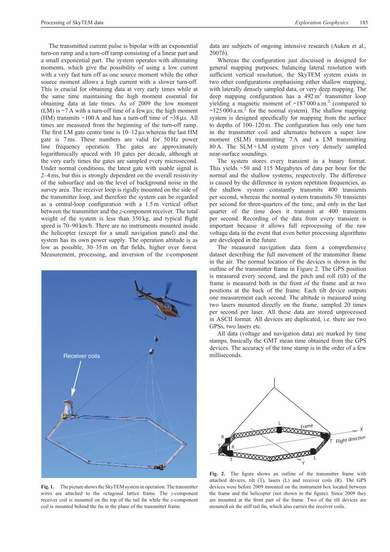
The transmitted current pulse is bipolar with an exponentialturn-on ramp and a turn-off ramp consisting of a linear part anda small exponential part. The system operates with alternatingmoments, which give the possibility of using a low currentwith a very fast turn off as one source moment while the othersource moment allows a high current with a slower turn-off.This is crucial for obtaining data at very early times while atthe same time maintaining the high moment essential forobtaining data at late times. As of 2009 the low moment(LM) is ~7A with a turn-off time of a fewms; the high moment(HM) transmits ~100A and has a turn-off time of ~38ms. Alltimes are measured from the beginning of the turn-off ramp.The first LM gate centre time is 10–12ms whereas the last HMgate is 7ms. These numbers are valid for 50Hz powerline frequency operation. The gates are approximatelylogarithmically spaced with 10 gates per decade, although atthe very early times the gates are sampled every microsecond.Under normal conditions, the latest gate with usable signal is2–4ms, but this is strongly dependent on the overall resistivityof the subsurface and on the level of background noise in thesurvey area. The receiver loop is rigidly mounted on the side ofthe transmitter loop, and therefore the system can be regardedas a central-loop configuration with a 1.5m vertical offsetbetween the transmitter and the z-component receiver. The totalweight of the system is less than 350 kg, and typical flightspeed is 70–90 km/h. There are no instruments mounted insidethe helicopter (except for a small navigation panel) and thesystem has its own power supply. The operation altitude is aslow as possible, 30–35m on flat fields, higher over forest.Measurement, processing, and inversion of the x-component

data are subjects of ongoing intensive research (Auken et al.,2007b).

Whereas the configuration just discussed is designed forgeneral mapping purposes, balancing lateral resolution withsufficient vertical resolution, the SkyTEM system exists intwo other configurations emphasising either shallow mapping,with laterally densely sampled data, or very deep mapping. Thedeep mapping configuration has a 492m2 transmitter loopyielding a magnetic moment of ~187 000 a.m.2 (compared to~125 000 a.m.2 for the normal system). The shallow mappingsystem is designed specifically for mapping from the surfaceto depths of 100–120m. The configuration has only one turnin the transmitter coil and alternates between a super lowmoment (SLM) transmitting 7A and a LM transmitting80A. The SLM+LM system gives very densely samplednear-surface soundings.

The system stores every transient in a binary format.This yields ~50 and 115 Megabytes of data per hour for thenormal and the shallow systems, respectively. The differenceis caused by the difference in system repetition frequencies, asthe shallow system constantly transmits 400 transientsper second, whereas the normal system transmits 50 transientsper second for three-quarters of the time, and only in the lastquarter of the time does it transmit at 400 transientsper second. Recording of the data from every transient isimportant because it allows full reprocessing of the rawvoltage data in the event that even better processing algorithmsare developed in the future.

The measured navigation data form a comprehensivedataset describing the full movement of the transmitter framein the air. The normal location of the devices is shown in theoutline of the transmitter frame in Figure 2. The GPS positionis measured every second, and the pitch and roll (tilt) of theframe is measured both in the front of the frame and at twopositions at the back of the frame. Each tilt device outputsone measurement each second. The altitude is measured usingtwo lasers mounted directly on the frame, sampled 20 timesper second per laser. All these data are stored unprocessedin ASCII format. All devices are duplicated, i.e. there are twoGPSs, two lasers etc.

All data (voltage and navigation data) are marked by timestamps, basically the GMT mean time obtained from the GPSdevices. The accuracy of the time stamp is in the order of a fewmilliseconds.Receiver coils

Fig. 1. The picture shows the SkyTEMsystem in operation. The transmitterwires are attached to the octagonal lattice frame. The z-componentreceiver coil is mounted on the top of the tail fin while the x-componentcoil is mounted behind the fin in the plane of the transmitter frame.

Fig. 2. The figure shows an outline of the transmitter frame withattached devices, tilt (T), lasers (L) and receiver coils (R). The GPSdevices were before 2009 mounted on the instrument box located betweenthe frame and the helicopter (not shown in the figure). Since 2009 theyare mounted at the front part of the frame. Two of the tilt devices aremounted on the stiff tail fin, which also carries the receiver coils.

Processing of SkyTEM data Exploration Geophysics 185

In the design and development of the SkyTEM system, theaim has been that the data quality should be the same as or betterthan the data quality of ground-based systems. One way ofaccomplishing this is to take several different ground-basedsystems to a reference site and make them reproduce eachother. Based on measurements from more than 10 different

Geonics Protem/TEM47 systems a ‘standard curve’ and a‘standard model’ have been established at a test site inDenmark. For the verification of the SkyTEM system we havecalculated a reference curve for the standard model fromwhich data are generated for the different dimensions of theSkyTEM transmitter loop, low-pass filters (Effersø et al., 1999),

250 500 750 1000 1250 1500 1750

0

Distance [m]

10

20

30[m]

[m/s]

[Deg]

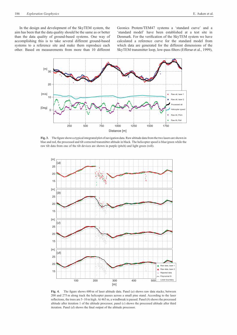
Fig. 3. Thefigure shows a typical integratedplot of navigationdata.Rawaltitudedata from the two lasers are shown inblue and red, the processed and tilt corrected transmitter altitude in black. The helicopter speed is blue/green while theraw tilt data from one of the tilt devices are shown in purple (pitch) and light green (roll).

(a)

(b)

(c)

(d )

20

25

15

[m]

20

25

15

[m]

20

25

15

[m]

20

25

15

[m]

[m]100 200 300 400 500

Raw data, laser 1

Raw data, laser 2

Rejected data

Polynomial fit

Lower boundary

Fig. 4. The figure shows 600m of laser altitude data. Panel (a) shows raw data stacks; between200 and 275m along track the helicopter passes across a small pine stand. According to the laserreflections, the trees are 5–10m high. At 465m, a windbreak is passed. Panel (b) shows the processedaltitude after iteration 1 of the altitude processor, panel (c) shows the processed altitude after thirditeration. Panel (d) shows the final output of the altitude processor.

186 Exploration Geophysics E. Auken et al.

ramps, and altitude. When acquiring data at different altitudeswe can show that the SkyTEM response compares to betterthan 5% to the response of the standard model (Sørensen andAuken, 2004) at any of these altitudes.

The data for the SkyTEM system consist of navigation dataand voltage data. The processing is implemented as a module inthe Aarhus Workbench (Aarhus Geophysics, 2009), which issoftware developed in-house. The Aarhus Workbench is acommon platform for working with geophysical, geological,and GIS data. It includes fully integrated modules forgenerating geophysical thematic maps, geo-statistic modelling,and visualisation on GIS maps. The SkyTEM processingsystem is fully integrated with the GIS component (MapX,MapInfo Inc.). This is extremely important when working indensely inhabited areas where long data sequences often haveto be culled because data are severely biased by coupling to man-made conductors (Danielsen et al., 2003).

SkyTEM data processing is a four-step process: 1) navigationdata are filtered and averaged automatically, and manualcorrections may also have to be applied to the altitude data; 2)voltage data are processed automatically, i.e. filtered andaveraged, and standard deviations based on the data stacks arecalculated; 3) voltage data are evaluated manually for furtherrefinement of the processing (necessary in areas with culturalresponses); and finally 4) a fast inversion using a smooth modelis used to fine-tune the processing done in steps 1 to 3. Theautomatic processing of SkyTEM data (steps 1 and 2) isdone using several routines that work on the different datatypes. Each of the steps described above is addressedindividually in the following sections.

Navigation data processing

As mentioned above, navigation data are filtered and averagedautomatically, and manual corrections are applied to the altitudedata if needed.

The result of the automatic processing is inspected usingprofile plots of flight time versus data value (tilt, altitude,voltage data, etc.). This is illustrated in Figure 3. The plot alsoshows various quality control parameters, e.g. flight speed,topography, tilt (pitch and roll), etc. Other parameters liketopography, transmitter current, transmitter temperature etc.can also be displayed. A key feature in the processing is theuse of an integrated interactive GIS map where the helicopterlocation is highlighted. Combined with proper GIS themes, it isin most cases possible to explain most features in data, e.g. thatthe sudden increase in altitude and somewhat coherent noiseis an effect of the helicopter crossing a power line, that the lasersget bad reflections because the helicopter is moving acrossa forest, etc.

Since navigation data are gathered with different timestamps and recorded with different sampling intervals, it isconvenient to have the output of the navigation dataprocessors interpolated to common fiducial times, at aninterval which is typically set to 0.5 s or 1.0 s depending onthe flight speed. The GPS positions are simply fitted with a2nd order polynomial with a length of 10 s therebyinterpolating them so that there is one GPS position perfiducial time. Positions are also relocated so they correspondto the centre of the transmitter frame.

The frame tilt processor – pitch and roll

The tilt is measured both in front of the frame and at theback of the frame. The tilt measurements are important

for the correction of the altitude measurements and asinput to the inversion when inverting both x- and z-componentdata.

1e-6

1e-5

1e-4

1e-7

Sig

nal l

evel

[V/m

2 ]

1e-4 1e-3

Time [s]

1e-8

Fig. 5. The figure shows a capacitively coupled dataset being culledbecause the sounding has sign changes (error bars shown in red) in theinterval before the signal reaches the noise floor. The noise floor is surveyspecific, but here it is 5e-9V/m2 at 1ms and defined as being proportionalto t�1/2. A typical noise level seen in surveys from around the world is in theinterval 5e-9–1e-8V/m2.

250 500

1e-14

1e-12

1e-11

1e-10

1e-9

1e-13

Sig

nal l

evel

[V/m

4 *A

]

Distance [m]

1e-15

Fig. 6. Illustration of the trapezoidal average windows seen as a greytransparent polygon along with the raw data stacks. Averages are narrow atearly times to avoid lateral smoothing of the near-surface geology andwide atlate times where the signal/noise ratio needs to be increased to obtain thedesired depth of penetration.


Data from the two tilt meters mounted on the stiffplatform carrying the receiver coils (Figure 2) are normallyused for the data processing. The tilt data are smooth andslowly varying due to the low frequency movements of theframe (see Figure 3). They are simply median filteredover intervals typically of 3 s and then interpolated to thefiducial times.

The altitude processor

The altitude of the transmitter frame and receiver coils ismeasured to distinguish the substratum from air, especially inhighly resistive areas. Good altitude estimates are necessary asthey 1) prevent shallow, false highly resistive artefacts in themodel and 2) give an accurate starting parameter and therebyhelp stabilise and speed up the inversion. Most problems indetermining the correct altitude using lasers are caused by thelaser beam not being reflected from the surface of the groundbut from leaves. These reflections are seen as abrupt reductions inaltitude as illustrated in Figure 4a.

To eliminate these reflections and to correct for the laserbeam not always being vertical, several correction steps aretaken. First, the altitude has to be calculated at the centre ofthe transmitter frame, second the altitudes need to be filtered,and third theyare averaged and the altitudeof the receiver coils arecalculated.

The first step is a simple geometric calculation. The secondstep deals with altitude filtering. The challenge is to design a

robust filtering scheme, which picks only the highest reflectionsassuming they come from the ground surface (through smallholes in the leaf-cover), and at the same time do not remove thereal altitude variations of the frame. We have designed a verysimple recursive filtering scheme, which has proven to be robusteven over dense forest with few reflections from the ground.Leaf reflections are simply removed by repeatedly fitting a high-order polynomial to the altitudes while removing outlying data.Typically, a 9th order polynomial is fitted in a least-squaressense to a length of 40–60 s of data. All data of range onemetre less than the polynomial prediction are culled, and theprocess is repeated, typically 7–9 times.

As seen in Figure 4, panels b, c, and d, the filter graduallyfinds the maximum reflections in the along-track interval200–275m while leaving all other data untouched. Thereflections from the windbreak at 465m are removed almostimmediately. The length of the polynomial and the order arenormally adjusted manually by trial and error, and one set ofsettings are determined for the entire survey. The time intervalhas to be sufficiently long to cover long strips with tree topreflections, and the polynomial degree must be sufficientlyhigh to leave the actual variations untouched by the filter. Therecursive filtering is very fast and the trial and error processdoes not take much time.

After running the recursive filter on each of the lasers,data from both lasers are merged and fitted with a 9th orderpolynomial of length 40 s, and the altitude of the transmittercoil is calculated at the fiducial times. Finally, the altitudes

(a) Raw data (b) Square average (c) Trapezoid average

1e-5 1e-4 1e-3

1 gate culled

1e-5 1e-4 1e-3

4 gates culled

Improved lateralresolution

Sig

nal l

evel

[V/(

m4*

A)]

Time [s] Time [s] Time [s]1e-5 1e-4 1e-3

1e-9

1e-10

1e-11

1e-12

1e-13

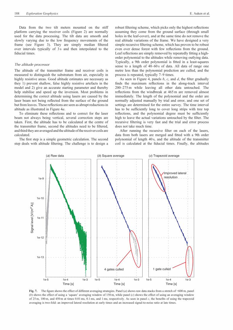
Fig. 7. The figure shows the effect of different averaging strategies. Panel (a) shows raw data stacks from a stretch of ~600m, panel(b) shows the effect of using a ‘square’ averaging window of 150m, while panel (c) shows the effect of using an averaging windowof 25m, 100m, and 450m at times 0.01ms, 0.1ms, and 1ms, respectively. As seen in panel c, the benefits of using the trapezoidaveraging is two-fold: an improved lateral resolution at early times and an increased signal-to-noise ratio at late times.


of the x- and z-receiver coils are calculated using the x-tilt(the pitch).

In a few cases, over very densely leaf-covered areas, therecursive filter does not output a reasonable estimate ofthe altitude, and in this case the user is free to manually drawthe altitude he or she prefers. However, our experience is that itis better in these cases to let the altitude be determined in theinversion (see below).

Processing of voltage data

High-quality data processing is a must in hydrogeophysicalsurveys; however, our experience shows that the sameapproaches can successfully be applied to most other types ofsurveys.

Voltages are divided into categories according to theirprocessing stage: 1) instrument data, e.g. raw un-stackedtransients from the receiver; 2) raw data, e.g. stacks oftransients (instrument data); and 3) averaged data, e.g.averages of raw data stacks.

The raw voltage data are collected with a certain number oftransients in the stack. The number of transients in the stack is setaccording to the desired signal-to-noise ratio and, equallyimportant, the power line frequency (and its most powerfulharmonics) is rejected. A typical stack size for the HM is96 transients, and for LM and SLM it is 160 or 320 transients.It takes 1.92 s (HM) and 0.64 s (LM and SLM) (1.28 s if320 transients) to complete these measurements and ~50ms to

change between the moments. When operating with the SLMand LM, an almost continuous sampling of the subsurface isachieved.

While the system alternates between LM+HMor SLM+LMin sequences of typically 10 pairs the 11th pair is used tomeasure the natural background level to assist the manual dataprocessing, as discussed below. This is simply done by turningoff the transmitter while the system still runs. In more remoteareas the noise measurements are typically done for each 20thor 30th pairs of moments.

While densely sampled data increase the amount of data tohandle, it also makes it possible to track rapidly shiftingsignal levels often seen in mineral exploration. SkyTEMvoltage data from the instrument are by default stacked duringimport, i.e. a raw data stack is created with the number oftransients mentioned above. However, depending on the targettype, it is possible to make a subdivision of the data stacks: i.e. tocreate a raw data stack for every 8, 16 or 32 transients. Theapplication of filters to the raw transients before stacking, tofurther increase the signal-to-noise level, is the subject ofongoing research. The x-component data, especially, showsignificant noise spikes, which are not efficiently suppressedby averaging only. Very useful noise-suppression techniquesare discussed by Macnae et al. (1984).

Data from areas with a significant amount of infrastructure,suchaspipes, power lines, andmetal fences, unfortunately requirea significant amount of manual processing, even though filtershave been designed to help cull disturbed data. These data are

10

20

30

40

50

Alti

tude

[m]

Alti

tude

[m]

1e-14

1e-12

1e-11

1e-10

1e-960

1e-13

(a) Raw data

Sig

nal l

evel

[V/m

4 *A

]S

igna

l lev

el [V

/m4 *

A]

Altitude data

Distance [m]

10

250 500 750 1000 1250 1500 1750

20

30

40

50

1e-14

1e-12

1e-11

1e-10

1e-960

1e-13

(b) Averaged data

Fig. 8. The figure shows 3min of HM data corresponding to ~2000m on the ground. The time gates range from 7.18e-5 s to 8.8e-3 s. Theflight altitude is illustrated with the black line in both panels. Panel (a) shows raw data while panel b) shows averaged data. The filteringwidth increases from 5 s to 12 s from the time gate in the interval 1e-4 s to 1e-3 s, then increases to 28 s at gate 1e-2 s. The non-spikefilter removes ~20% of the raw data. A removed capacitive coupling is seen from 500m to 850m. The flanks of culled averaged dataseen in panel (b) from 520 to 540m and 820 to 840m are caused by the trapezoidal averaging filter. The arrow indicates the location of thedata shown in Figure 7c. The results of inversion of this data are shown in Figure 9.


removed entirely from the raw stacks, as they will otherwise besmeared out and significantly degrade the quality of the datathat arenot influencedbycoupling.Danielsen et al. (2003)discussthe physics behind the galvanic and capacitive couplingphenomena. Designing filters to detect galvanic coupling isnot considered viable as the signal level is simply raised anddoes not show oscillation. A filter for detection of capacitivecoupling, which shows oscillations and possible sign changes,is easier to design. The capacitive coupling detection filterworks by examining both the raw data stacks for changes incurve slopes and sign changes within the time interval where auseful signal is to be expected. In other words, the detectionfilter is executed from the first gate of the sounding until thesignal reaches the noise floor. This is illustrated in Figure 5.

In most cases the entire data curve is removed even whereonly the late time gates (with signal above the noise level)are disturbed visually, i.e. they oscillate. This is done becausewe often see an unrealistic rise in signal (galvanic effect) beforethe actual oscillations. The noise level is estimated from themeasurements of the background noise.

Typically, all data within a distance of 100–150m fromroads, power lines, windmills, slurry tanks etc. must be culled.The exact distance depends on the subsurface conductivity.A low-conductive ground produces a low electromagneticresponse, which increases this distance, whereas a high-conductive ground produces a large signal, and the couplingdistance is decreased.

The raw data stacks are corrected for the reduction in theeffective of the transmitter and receiver when coils when thecoils are tilted. For the z-component data this is

db

dtcor¼ 2

db

dtcosðapitchÞcosðarollÞ; ð1Þ

where db/dtcor is the tilt corrected voltage, db/dt is the voltage,apitch is the pitch angle and aroll is the roll angle. Both the areaof the transmitter and the receiver loops are reduced, hencethe factor of 2. In itself this correction is just an areacorrection of the data, and it does not take into account thehorizontal components of the tilted transmitter, nor does itcorrect for the horizontal magnetic field in the receiver loop asdescribed for helicopter frequency domain data (HEM) inFitterman and Yin (2004). However, forward modelling of thefull system response has shown that, when the pitch and roll isbelow 15–20 degrees, the area correction is less than ~5%compared to the full solution which includes both z- and x-transmitter loops. For the normal operation, the pitch androll is less than 15 degrees, and the correction is thereforenegligible.

Designing an optimal data averaging scheme

The standard approach for airborne TEM is that data areaveraged over the same distance at early times and late times.The downside of this approach is that it is not possible tomaintain a high resolution at early times (corresponding tothe near surface), where the signal-to-noise ratio is usuallyrelatively high, and still obtain a reasonable signal-to-noiseratio at late times, i.e. at a large penetration depth.Furthermore, for quasi-layered environments, it must bestressed that a small sounding distance, e.g. 5m, does notnecessarily correspond to a high lateral resolution if data arestill averaged over long time spans or distances, e.g. 150m. Itjust means a high level of redundant information.

Our approach is to use trapezoidal average windows sothat early-time data are averaged less than late-time data, as

illustrated in Figure 6. This approach is actually an image ofthe nature of the electrical fields in the substratum itself. If asounding is produced e.g. at each 30m, the very early time datawill not be averaged over more than 30m, whereas late-timedata may be averaged over e.g. 300m. By doing this we 1)maintain the optimal resolution of the near-surface resistivitystructures, where the current system in the ground is relativelysmall and the signal-to-noise ratio good, and 2) obtain areasonable signal-to-noise ratio at late times, therebymaintaining the desired penetration depth. Deeper lyingstructures are averaged both by the larger current system andby the filters, but the amount of redundant information isminimized.

The actual width of the trapezoidal average filter is normallychosen as narrow as possible for the early-time gates to give thehighest possible unsmeared resolution of the near-surfaceresistivity structures. The late-time gates are averaged so thatthe desired depth of penetration is obtained while still retaininglateral resolution of the geological layers. Simulation of theaveraging filter has been carried out on synthetic 3D datagenerated over buried channel structures, data presented inAuken et al. (2008). The results show that late-time dataaveraged over up to 200m laterally do not change the invertedmodel significantly.

10 100

10

200

100

Dep

th [m

]

Resistivity [Ω.m]

1e-4 1e-2100

1000

1e-5

Res

istiv

ity [Ω

.m]

Time [s]

Fig. 9. Model curve showing the sounding from Figure 7c (red error bars)along with the forward response (red line). As seen, data are generally wellfitted. The model shows a thin (~10m) uppermost layer with a resistivityof ~40W.m, underlain by a layer of similar thickness and a resistivity of10W.m. Below this layer is found a thick high resistive layer (~100W.m)overlaying a ~10W.m layer. Geologically the model reflects from the top;till, clay rich till, sand/gravel (aquifer), and tertiary clay (aquitard).


The effect of late and early time averaging is illustratedin Figure 7. The raw data in Figure 7a are filtered andaveraged using a square averaging windows (Figure 7b) wheredata are averaged over ~150m at both early and late times, and atrapezoidal averaging window (Figure 7c) where data areaveraged over ~25m at 0.01ms, 100m at 0.1ms, and 450m at1ms. As expected, the increased averaging at late timesincreases the signal-to-noise ratio considerably, as indicated bythe grey data points showing which gates would be culled in anormal processing phase because of not meeting thedesired signal-to-noise ratio. In this case only one is culled forthe trapezoidal scheme and four for the square scheme.Furthermore, the use of a relatively wide averaging core atearly times, which is necessary to maintain at least areasonable signal-to-noise ratio at late times, means loss ofresolution at early times in the square case.

During this filtering the raw voltage data are not correctedfor variations caused by varying altitude over the averagingwindow. Such a correction would require a full inversionof the raw datasets, which would then be used for calculatinga set of correction factors to bring the response to anominal flight altitude. It can, however, be shown that theerror introduced by using an average can be neglected foraltitude changes less than 20m in the averaging window.

The average soundings are formed by applying a de-spikefilter for each time channel. Typically 20% of the raw datastacks (at each channel) are removed, and the rest are averagedwhile also calculating the standard deviation. Our experienceshows that the de-spiking is important, especially onx-component data where the raw data are characterised bynoise spikes of high amplitude and short duration. A typicaldata profile is shown in Figure 8. From 500 to 850m along trackthe helicopter crosses a road, and capacitive coupling is seen.These data have been removed from the raw data stacks asseen in Figure 8a. The last usable time gate in the averageddata (Figure 8b) is 0.88ms.

Inversion

Inversion of SkyTEM data is the subject of several otherpapers and abstracts (Viezzoli et al., 2007; Auken et al., 2008),and the intention of the following is therefore just to tie togetherthe processing and the inversion.

Using a smooth inversion for post processingof voltage data

Both in situations where a large part of the data are culled becauseof coupling, and in situations where the main noise source is the

250 500 750 1000 1250 1500 1750

Distance [m]

50

–200

0

–50

–100

–150

2

1

50

–200

0

–50

–100

–150

Ele

vatio

n [m

]E

leva

tion

[m]

2

1

Dat

a re

sidu

alD

ata

resi

dual

1 10010Resistivities [Ω.m]

(a)

(b)

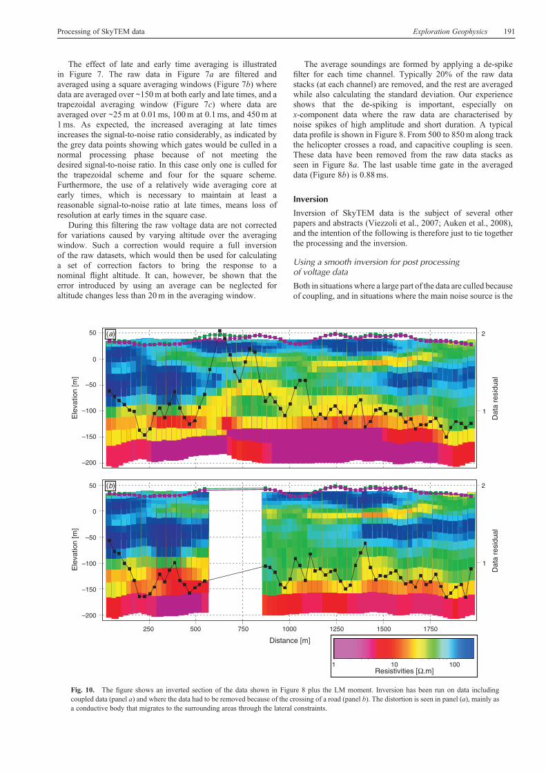
Fig. 10. The figure shows an inverted section of the data shown in Figure 8 plus the LM moment. Inversion has been run on data includingcoupled data (panel a) and where the data had to be removed because of the crossing of a road (panel b). The distortion is seen in panel (a), mainly asa conductive body that migrates to the surrounding areas through the lateral constraints.


natural background noise, we find it useful to run a smoothinversion of the average data as the final step in theprocessing. We use the Laterally Constrained Inversion (LCI)algorithm (Auken et al., 2005) for this. This inversion is used toremove outlier data that, for some reason, have not beenremoved in the automatic filters or the manual processing.Such data always occur at late times where the signal-to-noiselevel is low. Typically, data that deviate more than twice thedata standard deviation to the forward response of theinverted models are removed. As an example of a smoothinversion Figure 9 shows the results of inverting the data inFigure 7c. Data are converted to late time apparent resistivityto make it easier to evaluate the data fit. Data are well fitted atearly as well as late times.

Final inversion of data

The data standard deviation calculated from the data stack entersthe inversion scheme and is used basically to weight theindividual data points. The flight altitude is also treated as aninversion parameter, with an a priori uncertainty set at a fixednumber, typically �3m. Constraining the altitude no more than3m allows the inversion to move the altitude to its correct value,thereby not compromising the validity of the model.

The inverted section of the data in Figure 8 plus the LM data(not shown), are shown in Figure 10 along with data residuals(black line/dots) and input altitude (green line/dots) and outputaltitude (purple line/dots). Themodel has sixteen layerswithfixedthicknesses, and the LCI algorithm was set up with a lateralvariation from model to model of a factor of 1.5 for resistivities.The inversion was run both on data for which the distorted dataaround 500–850m had not been removed (Figure 10a) and ondata for which they had (Figure 10b). As expected, the majordifference in the results is around the centre of the distortion,which is seen mainly as a conductive body in panel a. In the LCI,due to averaging and the lateral constraints, this unwantedinformation migrates laterally to the surrounding areas therebydegrading the quality of these data. It is also seen from the dataresidual that data in this area are poorly fitted and that theinversion routine actively moves the altitude in order to fitdata. In Figure 10b, it is seen that data are generally fittedwithout needing move the altitude.

Conclusion

We have discussed the entire workflow of processing SkyTEMnavigation and voltage data. The navigation data include datafrom GPS receivers, frame pitch and roll, and frame altitude.Several steps are taken toobtainmaximumdataquality andby thisto get the most detailed possible resolution of the resistivitystructure of the subsurface. At all stages in the processing it isknow by the user what is done to the data and no system orprocessing parameters are proprietary.

Even though the raw voltage data are bias free, they need tobe corrected to account for the reduced horizontal transmitterand receiver areas when the frame moves in the air. Data areaveraged using trapezoidal average filters, and data are also de-spiked. The filters are designed so that the lateral resolution ofresistivity structures is least possible smeared. With this designthe lateral resolution of the shallow subsurface is maintainedthrough a narrow averaging of early-time data, whereas theoptimal penetration depth is achieved through a wider average.

We have argued that data which are influenced by coupling toman-made installations on the ground surface must beculled before entering the averaging scheme as, otherwise,good data are degraded. It is important that this is done by the

geophysicist processing the data, as he or she has the sourceinformation necessary to decide whether data are coupled or not.This information is not readily available after averaging andinversion.

Acknowledgement

Professor Kurt Sørensen has greatly contributed to the research presentedin this paper. We also need to thank the two reviewers, Dr A. Maddeverand one anonymous; their comments have made the manuscript mucheasier to read.

References

Aarhus Geophysics, 2009, Aarhus Workbench. Available online at:http://www.aarhusgeo.com/products/workbench.html (accessed 9 May,2009).

Auken, E., Christiansen, A. V., Jacobsen, L., and Sørensen, K. I., 2008,A resolution study of buried valleys using laterally constrainedinversion of TEM data: Journal of Applied Geophysics, 65, 10–20.doi: 10.1016/j.jappgeo.2008.03.003

Auken,E.,Westergaard, J.A.,Christiansen,A.V., andSørensen,K. I., 2007a,Processing and inversion of SkyTEM data for high resolutionhydrogeophysical surveys: 19thGeophysical Conference and Exhibition,Australian Society of Exploration Geophysicists, Extended Abstracts.

Auken, E., Foged, N., Christiansen, A. V., and Sørensen, K. I., 2007b,Enhancing the resolution of the subsurface by joint inversion of x- andz-component SkyTEM data. 19th Geophysical Conference andExhibition, Australian Society of Exploration Geophysicists, ExtendedAbstracts.

Auken, E., Christiansen, A. V., Jacobsen, B. H., Foged, N., andSørensen, K. I., 2005, Piecewise 1D Laterally Constrained Inversionof resistivity data: Geophysical Prospecting, 53, 497–506. doi: 10.1111/j.1365-2478.2005.00486.x

Danielsen, J. E., Auken, E., Jørgensen, F., Søndergaard, V. H., andSørensen, K. I., 2003, The application of the transient electromagneticmethod in hydrogeophysical surveys: Journal of Applied Geophysics,53, 181–198. doi: 10.1016/j.jappgeo.2003.08.004

d’Ozouville, N., Auken, E., Sørensen, K. I., Violette, S., Marsily, G. D.,Deffontaines, B., and Merlen, G., 2008, Extensive perched aquifer andstructural implications revealed by 3D resistivitymapping in a Galapagosvolcano: Earth and Planetary Science Letters, 269, 518–522.doi: 10.1016/j.epsl.2008.03.011

Effersø, F., Auken, E., and Sørensen, K. I., 1999, Inversion of band-limitedTEM responses: Geophysical Prospecting, 47, 551–564. doi: 10.1046/j.1365-2478.1999.00135.x

Fitterman, D. V., and Yin, C., 2004, Effect of bird maneuver on frequency-domain helicopter EM response: Geophysics, 69, 1203–1215.doi: 10.1190/1.1801937

Macnae, J. C., Lamontagne, Y., and West, G. F., 1984, Noise processingtechniques for time domain EM systems: Geophysics, 49, 934–948.doi: 10.1190/1.1441739

Munday, T., Fitzpatrick, A., Reid, J. E., Berens, V., and Sattel, D., 2007,Frequency and/or Time Domain HEM Systems for Defining FloodplainProcesses Linked to the Salinisation along the Murray River. 19thGeophysical Conference and Exhibition, Australian Society ofExploration Geophysicists, Extended Abstracts.

Reid, J. E., and Viezzoli, A., 2007, High-Resolution Near Surface AirborneElectromagnetics – SkyTEM Survey for Uranium Exploration at PellsRange, WA. 19th Geophysical Conference and Exhibition, AustralianSociety of Exploration Geophysicists, Extended Abstracts.

Sørensen, K. I., and Auken, E., 2004, SkyTEM? A new high-resolutionhelicopter transient electromagnetic system: Exploration Geophysics,35, 194–202. doi: 10.1071/EG04194

Viezzoli, A., Christiansen, A. V., Auken, E., and Sørensen, K. I. 2007,Spatially Constrained Inversion for Quasi 3-D Modelling of AEMData. 19th Geophysical Conference and Exhibition, Australian Societyof Exploration Geophysicists, Extended Abstracts.

Manuscript received 19 November 2008; revised manuscript received7 May 2009.


http://www.publish.csiro.au/journals/eg

An integrated processing scheme for high-resolution ...

Documents

Transcript of An integrated processing scheme for high-resolution ...