Generic Framework and Methods for Integrated Risk Management in ...

An Integrated Framework for Risk and Safety
Evaluation and Process Design
This thesis is presented for the degree of
Doctorate of Philosophy
by
Fakhteh Moradi
BE, Iran University of Science and Technology, 2001
School of Engineering and Energy
Murdoch University, Perth, Western Australia, 2010

ii
Declaration
I declare that this thesis is my own account of my research and contain as its main
content work which has not previously been submitted for a degree at any tertiary
education institution.
………………………….
Fakhteh Sadat Moradi

iii
Abstract
Safety evaluation and risk assessment in processing plants can improve the reliability of
systems and reduce the number of hazardous events or eliminate the undesirable
consequences of these events. Safety and risk study may be conducted at any stage of
the plant life cycle from the conceptual design to the operational phase. Although
performing safety improvement and risk treatment in any step of plant life would have
important benefits, only early consideration of risk and safety results in permanent and
fundamental impacts on the reliability of the system. Integration of safety assessment
into process design provides the opportunity to take preventive and proactive actions to
eliminate possible hazards. It allows to fundamentally enhance the safety status of the
plant rather than using passive add-on controls and taking corrective actions which were
common in traditional approaches. A number of works have addressed this topic
previously, however, few works have tried to develop an integrated framework to
implement both process design and safety assessment concurrently.
Petri net tool has been introduced and investigated in this study to achieve integration of
safety assessment and process design. The Petri net is a powerful graphical modelling
tool with the mathematical ability to implement multiple functions simultaneously.
Inherent safety assessment method and probabilistic risk analysis technique have been
combined to create a new measure for safety evaluation and risk assessment of the plant.
The integrated framework has been developed based on the implementation of the
combined method using the introduced Petri net tool. The proposed approach has the
capability to automatically generate all possible combinations of the basic unit
operations and the unit operations which are available for safety enhancement in a
processing plant.

iv
The performance of the integrated framework has been demonstrated and evaluated
through two case studies: an acrylic acid production plant and a gold processing plant.
The results with the outcomes of application of two well-known methods of inherent safety
assessment and probabilistic risk analysis confirmed the reliability of the proposed method.
It showed that the proposed approach has the ability to generate all possible process
options and execute the safety evaluation simultaneously. The final safety factor
calculated for each process option takes into account a wide range of safety and risk
aspects. This approach provides a more comprehensive safety and risk assessment in
comparison with the other existing methods. It was concluded that the proposed
framework is an efficient solution to safety consideration during the early design stages.

v
Contents
Declaration ii
Abstract iii
Contents v
List of Figures ix
List of Tables xi
Nomenclature xiii
Acknowledgements xvii
Publications xviii
1. Introduction
1.1 Background 1
1.2 Scope of the study 3
1.3 Structure of the thesis 3
2. Literature Review
2.1 Introduction 6
2.2 Definitions 6
2.3 Risk/safety assessment methods 7
2.3.1 General risk/safety assessment methods 11
2.3.2 Environmental risk/safety assessment methods 34
2.4 Concurrent safety analysis and process design 37
2.5 Risk/safety assessment implementation tools 40
2.6 Conclusion 49
3. Research Design

vi
3.1 Introduction 57
3.2 A Petri net tool 58
3.3 A combined safety assessment and risk analysis methodology 59
3.4 Research procedure 60
3.5 Conclusion 61
4. Tool Development
4.1 Introduction 63
4.2 Petri net 64
4.2.1 General Petri net 65
4.2.2 Timed Petri net 68
4.2.3 Modified place weighted Petri net 68
4.3 Acrylic acid case study 71
4.3.1 Acrylic acid production process 72
4.3.2 Petri net model 75
4.3.3 Inherent safety assessment method and I2SI indexing system 84
4.3.4 Discussion 95
4.4 Conclusion 96
5. Application of Other Petri Nets
5.1 Introduction 100
5.2 Stochastic Petri net 100
5.2.1 Stochastic Petri net and risk analysis 101
5.2.2 Case study 103
5.2.3 Discussion 109
5.3 Fuzzy Petri net 109
5.3.1 Fuzzy set theory and safety assessment 115
5.3.2 Fuzzy set theory and Petri net modelling 116
5.3.3 Case study 118
5.3.4 Discussion 124
5.4 Conclusion 125

vii
6. Methodology Development
6.1 Introduction 127
6.2 New methodology 128
6.2.1 Logical development 129
6.2.2 Mathematical development 130
6.2.3 Methodology enhancement 134
6.2.4 Tool enhancement 138
6.3 Application of the new methodology on the acrylic acid case study 139
6.3.1 Implementation and results 140
6.3.2 Discussion 145
6.4 Conclusion 146
7. Industrial Case Study
7.1 Introduction 149
7.2 The gold mining process 150
7.2.1 Kalgoorlie gold mines 152
7.2.2 Porgera gold mine 153
7.2.3 Beaconsfield gold mines 154
7.3 The gold mining Petri net model 155
7.4 Safety evaluation 158
7.4.1 Inherent safety assessment 159
7.4.2 Probabilistic risk analysis 159
7.4.3 Discussion 171
7.5 Conclusion 171
8. Conclusion and Future Research
8.1 Conclusion 174
8.2 Future research directions 177

viii
Appendices
Appendix A Indexing System 180
A.1 Integrated inherent safety index 180
A.2 Gold mining process input data 202
Appendix B C++ Codes 208
Appendix C Glossary Of Technical Terms 209

ix
List of Figures
4.1 A simple example of a Petri net model 66
4.2 Acrylic acid production route – basic option 74
4.3 Acrylic acid production route – the second option 74
4.4 Acrylic acid production route – the third option 74
4.5 Super-net model – acrylic acid case study 78
4.6 Sub-nets A, B, C and D included in the super-net model 79
4.7 Flowsheets of the 8 generated routes and respective Petri net models 84
5.1 Graphical representation of a fuzzy sets 111
5.2 Sugeno-style fuzzy inference 114
5.3 Graphical representation of a fuzzy Petri net 118
5.4 Fuzzy sets related to the Failure Rate variables 120
5.5 Fuzzy sets related to the Severity of the Consequences variables 121
5.6 Fuzzy sets related to the Safety Condition variables 121
7.1 Kalgoorlie gold mines flowsheet 153
7.2 Porgera gold mines flowsheet 154
7.3 Beaconsfield gold mines flowsheet 155
7.4 Super-net model – gold mining case study 156
7.5 Flowsheets of the 12 generated routes and respective Petri net models 170
A.1 Conceptual framework of the I2SI 181
A.2 Conceptual framework of the HI 182
A.3 Conceptual framework of the ISPI 183

x
A.4 (a) Damage index graph for fire and explosion. (b) Damage index graph for
acute toxicity. (c) Damage index graph for chronic toxicity
184
A.5 (a) Damage index graph for air pollution. (b) Damage index graph for water
pollution. (c) Damage index graph for soil pollution
187
A.6 Monograph for process and hazard control index (PHCI) 189
A.7 (a) Inherent safety index for Minimization guideword. (b) Inherent safety
index for Substitution guideword. (c) Inherent safety index for Attenuation
guideword. (d) Inherent safety index for Limiting Of guideword
190
A.8 Procedure to calculate losses 194
A.9 Framework for inherent safety cost computation 201

xi
List of Tables
2.1 Risk and safety assessment methods; specification summary 10
2.2 (a) Parameters listed by Edwards and Lawrance, (b) Temperature
scoring, (c) Pressure scoring, (d) Inventory scoring, (e) Explosiveness
scoring
19
2.3 (a) Chemical Inherent safety sub-indices, (b) Process Inventory safety
sub-indices
23
2.4 List of risk indices for a given chemical component 33
2.5 Rating value of the component‟s risk indices 34
2.6 List of inherent risk indices for a given unit operation 34
2.7 Risk and safety assessment implementation tools; specification
summary
42
4.1 Interpretation of all places in Figures 4.5 and 4.6 76
4.2 Input data not considering the cost factors 85
4.3 Summary of the results – not considering the cost factors 89
4.4 Input data considering the risk factors 91
4.5 Summary of the results – considering the cost factors 95
5.1 Guideline to quantify the magnitude of the consequences of the failure 104
5.2 Input data in the stochastic Petri net case study 105
5.3 Summary of the results – stochastic Petri net case study 109
5.4 Linguistic variable of Failure Rate 119
5.5 Linguistic variable of Severity of the Consequences 119
5.6 Linguistic variable of Safety Condition 120
5.7 Matrix of fuzzy rules 122

xii
5.8 Fuzzy rules 122
5.9 Summary of the results – fuzzy Petri net case study 125
6.1 Severity of the consequences normalised within the range of [1,200] 134
6.2 Modified input data related to the unit operations in PRA method 141
6.3 Places‟ weight factors and transitions‟ firing rates 141
6.4 Summary of the results – new methodology 145
7.1 Interpretation of all places in Figure 7.4 157
7.2 Interpretation of all common sub-nets and respective places 158
7.3 Input data – inherent safety assessment 160
7.4 Input data - probabilistic risk analysis 161
7.5 Summary of the results – application of the proposed method on gold
mining case study
170
A.1 Guideline to decide extent of requirement of control arrangements 188
A.2 Guidelines to decide the extent of applicability of inherent safety guidewords 191
A.3 Guidelines to decide ISI value for guideword simplification 191
A.4 Range of cleanup costs for different chemical types 197
A.5 Classification of process control measure costs 198
A.6 Classification of add-on safety measure costs 199
A.7 Gold mining input data- I2SI and its two main sub-indices: ISPI & HI 202
A.8 Input data for the calculation of ISI 203
A.9 Input data for the calculation of PHCI 204
A.10 Input data for the calculation of DI 205
A.11 Input data for the calculation of PHCI after implementing inherent safety
principles
206

xiii
Nomenclature:
A………………………………………………………………...………….…Attenuation
ac………………………………………………………………...…………Acute toxicity
AL…………………………………………………………………….…..……Asset Loss
b………………………………………………………………………………….Blastwall
C…………………………………………………………………………..………….Cost
c…………………………………………………………………….………Concentration
CCA……………………………………...……...…………Cause-Consequence Analysis
ch………………………………………………………….………...……Chronic toxicity
CI…………………………………..…………..…….Chemical Inherent/Chemical Index
CIL………………………………………………………………..……..Carbon In Leach
CIP………………………………………………………...………..……..Carbon In Pulp
COR…………………….………………………………………….……….Corrosiveness
CP…………………….……………………………………………….Cleaner Production
CSCI…………….……………………………………….Conventional Safety Cost Index
d……………………………………………………………..……………Forced Dilution
DA…………..…………………………………………………..Diagraph-based Analysis
DI…………………………………………………………………....……..Damage Index
Dist…………………………………………………………………..…...……Distillation
Dr ………………………………………………………………………………… Doctor
DTA……………………………………………………..………Decision Table Analysis
ECC………………………………………………………...Environmental Cleanup Cost
EIM…………………………………………………Environmental Impact Minimization
en…………………………………………………..……...………Environmental damage
Env………………………………………………………...………………Environmental
EQ/Equ………………………………………………………………….……..Equipment
Eq………………..……………………………………………………………….Equation

xiv
ETA…………………………………………………………….……Event-Tree Analysis
EX………………………………………………………………..…..…….Explosiveness
f……………………..…………………………………………………………….….Flow
fe………………………………………………………...…………….Fire and Explosion
FI……………………………………………………………...………….Flowsheet Index
FL……………………………………………………………….…………..Flammability
FMEA………………………………………...……….Failure Mode and Effect Analysis
FMECA…………………………..………..Failure Mode and Effect Criticality Analysis
fr………………………………………………………………….…...…..Fire Resistance
FTA……………………………………………………..……………Fault-Tree Analysis
GERA………………………………..………….Global Environmental Risk Assessment
GUI…………………………………………………..……...…..Graphical User Interface
HAZOP……………………………………………….…………..Hazard and Operability
HCI………………………………………………….……………Hazard Chemical Index
HHL………………………………………………..………………...Human Health Loss
HI……………………………………………..……………….…..Hazard potential Index
HRI……………………………………………..…………………Hazard Reaction Index
I/i……………………………………………………………...…………………Inventory
I2SI……………………………………...………………Integrated Inherent Safety Index
ICI……………………………………………...……………..Individual Chemical Index
IEI……………………………………………….…………..Individual Equipment Index
INT………………………………………………………………..……………Interaction
IRI…………………………………………..………………….Individual Reaction Index
ISBL………………………………………………………………..Inside Battery Limit
ISCI…………………………………………………………...Inherent Safety Cost Index
ISD…………………………………………………………………Inherent Safer Design
ISI……………………………………………….………………….Inherent Safety Index
ISPI………………………………………..……………...Inherent Safety Potential Index
iv……………………………………………………………..……………...Inert Venting
L…………………………………………………...………………...Limitation of effects
l……………………………………………………………………...………………Level

xv
LCA……………………………………………………….………….Life Cycle Analysis
LCFMEA…………………………………………...…………….Life Cost-based FMEA
LEL…………………………………………………...…………..Lower Explosive Limit
LOPA………………………………………….…………...Layer Of Protection Analysis
M………........................................................................................................Minimization
MAX/max……………………………………………………………...……….Maximum
MEN…………………………………………………………….Mass Exchange Network
NFPA…………………………………..……………….National Fire Protection Agency
Num……………………………………………………………….………………Number
OCI………………………………………………………………Overall Chemical Index
ORA………………………………………………..……………...Optimal Risk Analysis
OSBL……………………………………………...……………….Outside Battery Limit
OSI………………………………………………….……………….Overall Safety Index
P/p…………………………………………………………………….…………..Pressure
PHA………………………………………...………………Preliminary Hazard Analysis
PHCI……......................................................................Process and Hazard Control Index
PhD…………………………………………………………………Doctor of Philosophy
PI…………………………………………………………Process Inherent/Process Index
PIIS……………………………………...……………Property Index for Inherent Safety
PL………………………………………………………………………...Production Loss
PP……………………………………………………………………Pollution Prevention
PRA………………………………………..…………………Probabilistic Risk Analysis
RM………………………………………………………...……………….Main Reaction
RS…………………………………………………………………………..Side Reaction
S……………………………………………………………...……………….Substitution
s………………………………………………………............................Sprinkler System
S……………………………………………………………….……………….Simulation
SD……………………………………………..………………..Sustainable Development
Si…………………………………………………………...………………Simplification
SRA……………………………………….……………...Subjective Reasoning Analysis
ST………………………………………………………………………………..Structure

xvi
T/t.....…………………………………………………………………......…..Temperature
TCI…………………………………………………………………Total Chemical Index
TOX……………………………………………………………………..………..Toxicity
TPN………………………………………………………………..……..Timed Petri Net
UEL……………………………………………………...………..Upper Explosive Limit
WAR…………………………………………………………Waste Reduction algorithm
WCI………………………………………………….…………….Worst Chemical Index
WM…………………………………………………….…………….Waste Minimization
WRI…………………………………………………...……………Worst Reaction Index
y………………………………………………………………………….…………..Yield

xvii
Acknowledgements
First and foremost I offer my sincerest gratitude to my supervisor, Professor Parisa A.
Bahri , who has supported me throughout my thesis with her patience and knowledge.
One simply could not wish for a better or more supportive supervisor.
I am delighted to thank the staff and students at the School of Engineering and Energy at
Murdoch University. I would particularly thank Bronwyn Phua and Roselina Stone for
their kind help with administrative matters.
I should also thank my dear friend Dr Mahsa Ghaeli for her support specially at the
initial stages of this research. Thanks to Dr Sally Knowles for proofreading my thesis
and her useful suggestions.
My very special appreciation goes to my dearest friend and sister Fatemeh for always
standing by me although thousands miles away.
I would like to express my deepest gratitude to my husband Reza for his absolute love
and support and my parents who have been constant source of encouragement and
unconditional love. I am also grateful to my family and friends for their caring attitude
during this period.
Finally, I would like to thank the School of Engineering and Energy at Murdoch
University for funding this research.
I apologise to those whose contributions, inadvertently, have not been acknowledged.

xviii
Publications
Several parts of the work and ideas presented in this thesis have been published by the
author during the course of the research or are under preparation and review to be
published. These publications are listed below.
Moradi, F & Bahri, P.A. 2008, „Development of a novel Petri net tool for process design
selection based on inherent safety assessment method‟, in Proceeding of the 18th
European Symposium on Computer Aided Process Engineering (ESCAPE 18), Lyon,
France, 2008, pp. 127-133.
Moradi, F & Bahri, P. A. 2009, „New safety evaluation methodology; A gold mining
application‟, in Proceeding of The 6th
International Symposium on Risk Management
and Cyber-Informatics: RMCI 2009, Orlando, Florida, USA, 2009, pp.
Moradi, F & Bahri, P.A. 2010, „A comprehensive survey on existing safety assessment
and risk evaluation methods with industrial application: Introducing a new tool‟, to be
submitted.
Moradi, F & Bahri, P.A. 2010, „Petri net, a capable safety assessment tool: An industrial
application‟, to be submitted.
Moradi, F & Bahri, P.A. 2010, „An integrated framework for safety evaluation and
process design‟, to be submitted.

Chapter 1. Introduction 1
CChhaapptteerr 11
IInnttrroodduuccttiioonn
1.1 Background
Although risk analysis and safety assessment methods have been applied in various
forms for many years, interest has increased recently among industries in developing
more efficient methods. Factors such as increased population density near industrial
complexes, larger size of operations, higher complexity and use of extreme operating
conditions, in addition to increased public concern for safety issues have led plant
designers to investigate the development and use of better hazard identification and
analysis techniques (Palaniappan et al., 2004). Moreover, because of the increase in
workplace automation, the safety evaluation has become more and more complex
(Vernez et al., 2004). Nowadays, the consideration of environmental problems plays an
ever-increasingly important role in chemical process design as well. The last decade of
the 20th
century saw significant progress made in industrial activities concerning
environmental issues (Hoyningen-Huene et al., 1999).
Integration of the safety analysis and design phase of a plant life cycle introduces
numerous benefits such as making the process permanently safer and reducing the need
for corrective actions, repair work and replacement. Considering the competitive
market, huge replacement and repair costs, limited availability of human expertise and
time constraints, concurrent safety analysis and process design can be of great
assistance. It can be through an automated process which reduces the need for human

Chapter 1. Introduction 2
intervention and the probability of human errors. Early identification of possible hazards
provides the opportunity to make efficient modifications prior to the implementation
phase. Consequently, a great amount of time and expenses related to taking corrective
actions are saved. Moreover, application of an integrated framework results in designing
a fundamentally safer process option which means reducing the probability of
irrecoverable human injuries and environmental damage.
While concurrent safety analysis and process design offers several benefits a very well-
defined and systematic approach is required to properly achieve it. There are a number
of factors that make it complicated. A proper methodology to be used for this purpose
needs to have specific characteristics. It has to rely on limited process data which is
available in the initial design phases. In the mean time, the results of risk and safety
evaluation have to be accurate to an extent to be usable as decision-making factors. The
other complicating issues are the required level of flexibility and simplicity for
methodologies and tools. The approach must be simple enough to not require special
expertise. It also has to have the flexibility of being applied in different systems, deal
with various input data and perform efficiently. These are the main issues faced in the
development of an integrated framework for safety evaluation and process design.
Past researches have mostly focused on identifying the approaches which can properly
analyse safety levels of a production route. However, recent researches are giving
special importance to the potential applicability of the safety assessment methods in the
early design stages. Surviving in the highly competitive market requires extra efforts.
One of the major necessities is being fast in modifications and precise in entering into
market and the other one is keeping the plants‟ lifetime cost reasonably low to be able to
compete in the market. Early safety evaluation would result in recognising the needed
modifications before time. Hence, the time and cost required for taking corrective
actions would be saved. Moreover, it will provide the opportunity of creating proactive
safety features instead of passive control options and lead to designing fundamentally
safer process alternatives which again means cut down on the time and cost of the
corrective actions. However, with the rapid growth in the number of the competitors and

Chapter 1. Introduction 3
the harsh market situation, integrated safety analysis and design process has become
more popular (Sherwin & Jonsson, 1995).
1.2 Scope of the study
The overall objective of this research was to develop an integrated safety evaluation and
process design method applicable to process industry. The sub-objectives are briefly
described as follows:
1. To provide an exhaustive survey of the literature directed towards the applicable
safety and risk analysis methodology in the process industries and an
investigation of their evaluation techniques and implementation tools.
2. To identify the available approaches with the technical potential to be applied
concurrently with the process design phase and investigate their limits and
strengths.
3. To identify the appropriate tools to implement the integrated safety evaluation
and process design and to make required modifications to enhance their
performance.
4. To develop a robust methodology to enable the development of an integrated
framework and cover a wide range of safety aspects.
5. To examine and illustrate the performance of the proposed tool and methodology
via visiting different case studies.
1.3 Structure of the thesis
An exhaustive literature survey is given in Chapter 2. This survey addresses the most
important safety and risk evaluation methodologies and tools with applications in
process industry.
Chapter 3 explains the general procedure which is followed in this study to achieve the
main objectives.

Chapter 1. Introduction 4
Chapter 4 provides details on Petri net tool which is an appropriate tool. This chapter
highlights the strengths of the Petri net tool and emphasises its suitability to the current
research by revisiting a case study adapted from the literature.
Chapter 5 investigates different types of Petri net tools in more detail. Stochastic Petri
net and fuzzy Petri net and their application in safety and risk evaluation are studied to
evaluate the ability of this tool to be applied in different systems.
Building on the previous chapters, Chapter 6 explains why inherent safety assessment
and probabilistic risk analysis are suitable techniques to be used as bases of the
methodology development. Then, the process of developing the new methodology is
explained step-by-step. The efficient performance of the proposed method and
developed tool is tested through undertaking the previous case study.
An industrial application of the proposed approach is illustrated in Chapter 7. Three
different gold production processes using various technologies are considered as basic
options for further investigation in this case study.
Finally, the study is summarised and discussed in Chapter 8. Significance of the
achieved results is outlined and possible further research and investigations are
suggested.

Chapter 1. Introduction 5
Reference
Hoyningen-Huene, P., Weber, H., & Oberheim, E. (1999). Science for the twenty-first
century, A new commitment Paper presented at the Conference Name|. Retrieved
Access Date|. from URL|.
Palaniappan, C., Srinivasan, P., & Tan, R. (2004). Selection of inherently safer process
routes: a case study. Chemical Engineering and Processing, 43(5), 641-647.
Sherwin, D. J., & Jonsson, P. (1995). TQM, maintenance and plant availability. Journal
of Quality in Maintenance Engineering, 1(1), 15-19.
Vernez, D., Buchs, D. R., Pierrehumbert, G. E., & Bersour, A. (2004). MORM-A Petri
Net Based Model for Assessing OH&S Risks in Industrial Processes: Modeling
Qualitative aspects. Risk Analysis, 24, 1719-1735.

Chapter 2. Literature Review 6
CChhaapptteerr 22
LLiitteerraattuurree RReevviieeww
2.1 Introduction
In this chapter a brief literature review of the risk and safety analysis is given. Since this
is a relatively wide area of research the literature on this topic is extensive. The scope of
literature review in this study is limited to risk and safety evaluation methods with the
potential of being applied in process industries.
Section 2.2 defines some important concepts in this area. Subsequently, Section 2.3
reviews the literature in the area of safety and risk analysis methods. Different
approaches in classification of these methods are presented in this section. Finally, the
chapter concludes in Section 2.4 with a discussion on shortcomings of applicable
methods of risk and safety assessment in process industries.
2.2 Definitions
Hazard: In this thesis generally, a hazard is an event that can result in any kind of
injury, fatality, damage and loss of time and/or money (Main, 2004). An environmental
hazard specifically, is any exposure to hazardous materials followed by harm to human
health or the environment (Achour et al., 2005).
Risk and safety: Risk can be defined as the product of probability of occurring any
potential hazard and the severity of its consequences. Safety is the condition of being

Chapter 2. Literature Review 7
protected against occurring of potential hazards and/or their consequences. In other
words, the reciprocal of safety is risk (Main, 2004).
Risk/safety assessment method: In this study, any approach, procedure or technique
that attempts to evaluate risks or safety associated with a process can be considered as a
risk or safety assessment method.
Risk/safety assessment tool: The techniques or approaches that help with systematic
and/or automated implementation of the risk/safety assessment methods in processes are
referred to as risk/safety assessment tools.
2.3 Risk/safety assessment methods
There are many approaches for the risk or safety analysis of workplaces. Based on the
specific purpose of each approach, it may focus on some particular aspects of safety in
production plants and be implemented through different techniques and tools
(Lichtenstein, 1996).
Risk and safety assessment methods come into two main groups of methods with
general application or with specifically environmental application. In each of these main
groups, different classes of qualitative, quantitative and semi-quantitative methods can
be recognised. Moreover, the risk and safety assessment techniques can be categorised
based on their compatibility with top-down and/or bottom-up approaches. An overall
view of these classifications are given in Table 2.1. Depending on the type of results
required from safety analysis process and the accessible input safety data, one of these
categories would be more suitable and applicable. These classes and approaches are
briefly explained as follows:
Quantitative methods: The purpose of quantitative safety analysis is to provide the
system designers with the quantified measures to assess safety and risk associated with
the system. Quantified measures are easy to use and understand and provide clear

Chapter 2. Literature Review 8
comparison base to compare different systems according to their risk and safety levels.
Quantitative techniques are generally resource demanding and require accurate
statistical data. On the other hand, application of these methods usually ends up with
deeper understanding of the system and more detailed information for further system
improvement (Ruxton, 1997).
Qualitative methods: This category of safety assessment methods is suitable to identify
possible failure events and suggest required safety guards to minimize the frequencies
and/or moderate the associated consequences with each event. Instead of using
numerical data some linguistic ranges may be used to measure the possibility of
occurrence of a hazard and the severity of the consequences of that hazard. An example
of these ranges is „catastrophic‟ to „negligible‟ for the severity of consequences and
„frequent‟ to „remote‟ for the probability of occurrence of a hazard (Ruxton, 1997).
Semi-Quantitative methods: The same as quantitative methods these methods are
based on identification of risk parameters and possible losses and include most of the
advantages of the quantitative methods. However, this category of approaches is not as
precise as quantitative methods and consequently it is not as resource intensive
(Bhimavarapu & Stavrianidis, 2000). Instead of using accurate numerical data the
majority of methods in this category apply different indexing systems to convert
qualitative concepts into quantitative measures.
Efficient use of safety analysis methods in the design stage involves the study of the
characteristics of each safety analysis method and the characteristics of the process
design. Two general approaches are available to implement different qualitative,
quantitative and semi-quantitative safety assessment methods based on characteristics of
systems under study. These approaches are described as follows:
Top-down Approach: A top-down analysis is based on identification of the critical top
events while further study is required to define the hierarchy of causes from the top level
to the lower level. This process continues to reach the appropriate level of causes

Chapter 2. Literature Review 9
(Ruxton, 1997). Both qualitative and quantitative analysis approaches can be applied to
estimate and evaluate the risk in a top-down design for safety process. The Fault-Tree
analysis method is an example of a typical top-down method.
Bottom-up Approach: The break down of a system to its subsystems and the
components of each subsystem to identify all possible hazards is the logic that bottom-
up analysis is based on. All possible hazards are identified at the bottom level up to the
top one and then a risk evaluation can be undertaken based on identified hazards
(Ruxton, 1997).

Chapter 2. Literature Review 10
Table 2.1 – Risk and safety assessment methods; specifications summary
Inheren
t Safety
Desig
n
Life C
ycle A
ssessmen
t
Total S
ite Analy
sis
Mass E
xch
ange N
etwork
s
Waste R
eductio
n alg
orith
m
Life C
ost-b
ased F
ME
A
Lay
er Of P
rotectio
n A
naly
sis
Pro
bab
ilistic Risk
Analy
sis
Sim
ulatio
n
Subjectiv
e reasonin
g A
naly
sis
Diag
raph
-based
Analy
sis
Decisio
n T
able an
alysis
Cau
se-Con
sequen
ce Analy
sis
Even
t-Tree A
naly
sis
Fau
lt-Tree A
naly
sis
Hazard
and O
perab
ility S
tudies
Failu
re Modes &
Effects A
naly
sis
Prelim
inary
Hazard
s Analy
sis
Meth
od
Risk
and safety
assessmen
t meth
ods
√ √
√
√
√
√
√
√
√
√
√
√
√
√
Gen
eral
Applicatio
n area
√
√
√
√
√
√
√
√
√
√
√
√
√
√
√
√
√
√
Env
.
√ √
√
√ √
√
√
√
√
√
Qualitativ
e
Classificatio
n
√ √ √
√ √
√
√
√
Quan
titative
√
√
√ √ √
Sem
i-quan
titative
√ √
√ √
√ √ √
√
√
Top
-dow
n
Com
patib
le appro
ach
√ √
√
√
√
√
√
√ √ √
Botto
m-u
p

Chapter 2. Literature Review 11
2.3.1 General risk/safety assessment methods
Several basic quantitative and qualitative techniques for risk/safety analysis are
identified in the literature. Moreover, ever-increasing importance of this science and
rapid advancement of engineering technologies is leading to development of many
innovative approaches in this area. In addition to basic methods several new approaches
are usually being created through merging two or more basic techniques or modifying
them by adding some features in order to ease their application, overcome their
limitations, improve their efficiency and/or speed up their performance.
The major basic techniques and some of the second generation methodologies are
described briefly in this section:
Preliminary Hazards Analysis (PHA): this is a qualitative technique which involves a
disciplined analysis of the event sequences that could transform a potential hazard into
an accident (Andrews & Moss, 1993). Event identification is the first step which is
followed by more detailed studies to find preventive and corrective measures for the
hazardous events and their consequences (Ruxton, 1997).
Failure Mode & Effect Analysis (FMEA/FMECA): this procedure based qualitative
method tries to analyse each potential failure mode in a system and determine its effect
on the system then classify it according to its severity (Andrews & Moss, 1993). Failure
mode and effects criticality analysis (FMECA) is the extended version of FMEA which
includes criticality analysis. It is probably the most widely applied hazard identification
method in the industries. The severity of the identified impacts may be defined by
linguistic variables such as: catastrophic, critical, marginal and negligible (Ruxton,
1997).
Hazard and Operability Studies (HAZOP): this qualitative method is a systematic
critical examination of the process and a series of engineering actions on new or existing
facilities to evaluate the hazard potential resulting from deviation in specifications and
their effects on the facilities. A set of guidewords is used in this method to identify

Chapter 2. Literature Review 12
hazardous situations or operational problems (American Institute of Chemical
Engineers, 1989; Andrews & Moss, 1993; Suokas & Rouhiainen, 1993; Sutton, 1992).
The HAZOP methodology introduces a better chance of detecting failure modes than
other alternative methods used in the risk identification phase in chemical process plants
(Ruxton, 1997).
Fault-tree Analysis (FTA): this method uses a deductive reasoning logical diagram
which shows the relation between system failure such as a specific undesirable event in
the system, and the failures of components of the system (Aven, 1992). An undesirable
event or an event with severe consequences is usually the top event of the logic diagram
in FTA. The failure events that lead to the top event are located immediately below in
successive levels of diagram. Each chain of failure events in a fault-tree diagram
represents a failure mode which causes the top event to happen (Ruxton, 1997). The
fault-tree can be used in qualitative and quantitative risk analysis (Sutton, 1992).
Event-tree Analysis (ETA): this method is used to show the sequence of events that
may occur after an identified initial event (American Institute of Chemical Engineers,
1989; Suokas & Rouhiainen, 1993; Sutton, 1992). ETA is based on inductive bottom-up
logic in which quantitative analysis can be carried out to assess the probability of
occurrence of each possible resulting consequence (Ruxton, 1997).
Cause-Consequence Analysis (CCA): this method combines cause analysis (FTA) and
consequence analysis (ETA) to take advantage of the strengths of both deductive and
inductive analysis methods. The purpose of CCA is to identify chain of events that may
result in undesirable consequences. Using the likelihood of events, the probabilities of
the consequences can be calculated (American Institute of Chemical Engineers, 1989;
Aven, 1992; Fullwood & Hall, 1988; Henley & Kumamoto, 1996; Suokas &
Rouhiainen, 1993).
Decision Table Analysis (DTA): this method contains a Boolean table and can be
considered as an automatic fault-tree construction technique. The Boolean table

Chapter 2. Literature Review 13
represents the whole engineering system based on its components, input events, output
events and their interactions. Boolean modelling is a bottom-up method that starts at the
lowest level of the system and continues to the appropriate upper levels. The concluding
table comprises all possible top events and associated cut sets. This modelling technique
provides a manageable representation of the failure modes associated with systems
containing multiple state components (Joshua & Garber, 1992; Kuhlman, 1977; Sutton,
1992).
Digraph-based Analysis (DA): this method uses the mathematics and language of
graph theory such as „path set‟ (Fullwood & Hall, 1988). It operates based on AND/OR
gates and different matrices to convert the graph language into mathematical
representations. It shows if a fault node will lead to the top event. DA is a bottom-up
event-based qualitative technique which allows cycles and feedback loops that make it
attractive for dynamic systems (Ruxton, 1997).
Subjective Reasoning Analysis (SRA): this method uses fuzzy set as the modelling
technique which is appropriate for measuring safety and hazard parameters concerning
their uncertain nature. Subjective reasoning is highly practical for modelling the systems
with unstable situation (Ruxton, 1997).
Simulation (S): different quantitative and qualitative simulation techniques have been
used in risk assessment of dynamic systems. These methods usually deal with AND/OR
logic and used together with other formal safety analysis such as FTA, ETA, CCA, and
FMEA to carry out quantitative analysis. Mont Carlo simulation method is an example
of this kind of technique (Ruxton, 1997).
Quantitative simulation: several quantitative simulation algorithms are available
to deal with systems with different failure distributions for which deterministic
methods are not suitable. This method is usually used with other techniques such
as FMECA, FTA, ETA and CCA to obtain different failure cut sets through
simulation of basic failure. Computer simulation methods are useful to calculate

Chapter 2. Literature Review 14
the probability of occurrence of the top event and its related cut sets (Ruxton,
1997).
Qualitative simulation: this inductive method is mainly suitable for risk
identification and the risk estimation phases in conjunction with previously
described methods such as FTA (Bell et al., 1992; Fullwood & Hall, 1988).
Probabilistic Risk Analysis (PRA): this method is based on potential major scenarios
with adverse impacts on the safety of a system. Two typical parameters need to be
obtained in PRA. The recognized hazardous scenarios need to be investigated and the
probability of their occurrence and magnitude of their consequences should be identified
for each unit operation and piece of equipment. The probability of occurrence of each
system failure event may be calculated on the basis of the identified cut sets and failure
probability data of the associated basic events. The cut set is a collection of basic events
which their occurrences lead to happening of top event (J. Wang & Ruxton, 1998).
Severity of consequences may be measured by considering possible loss of life and
property damage and the degradation of the environment caused by the failure event
(Ruxton, 1997). Different resources may be used to obtain required information for
risk/safety calculation such as experts‟ opinions, statistical data and experimental
results. Risk/safety level can be quantified using Bayesian probability theory
(Apostolakis, 1990). A simple two term equation may be used to calculate the risk factor
related to each unit operation/piece of equipment (Eq 2.1). Total risk associated with
each process option is given through summation of risk factors of all units included in
that option (Eq 2.2) (Bhimavarapu & Stavrianidis, 2000).
Risk = failure rate × consequences (Eq 2.1)
(Eq 2.2)
Where
i=0, …, n indicates the unit operation/equipment.

Chapter 2. Literature Review 15
Layer of Protection Risk Analysis (LOPA): this semi-quantitative risk analysis
technique defines the number of required protection layers in a system based on an
initial qualitative hazard identification usually through PHA and HAZOP. LOPA
focuses on pairs of cause-consequence scenarios and creates a numerical estimation of
the probability of the occurrence and estimates the frequency of the consequences
(Dowell & Hendershot, 2002). This quick and straightforward method quantifies the
expected failure rate of initiating cause and the probability of failure on demand of the
safeguards to define the frequency of consequences. In case of dependent failures and
lack of failure rate data this method can not be implemented efficiently. This limitation
can be overcome using FTA which is more complicated and time consuming but is
capable of evaluating interdependent and compound failure events. Combining LOPA
with FTA will provide the opportunity to take advantage of technical strength of FTA
while not sacrificing the simplicity of LOPA (Rothschild, 2005).
Optimal Risk Analysis (ORA): developing HAZOP method and equipping it with
some additional steps and analysing techniques has led to the creation of ORA. This
method comprises four main steps. The first step is a quick identification of process and
potential hazards considering chemicals, unit productions and conditions which results
in the generation of a list of units that require detailed analysis. HAZOP is used in
second step for detailed risk assessment. A computer automated tool is used to carry out
HAZOP which is based on FTA. The third step involves consequence evaluation in
order to quantify impacts of possible accidents using mathematical models and
simulations such as source model, models for explosions and fires and the impact
intensity models. Risk estimation is the concluding step. Based on estimated risk and
potential hazards, hazard-reduction policies are developed in this step (Khan et al.,
2001).
Life Cost-Based FMEA (LCFMEA): the main problem of traditional FMEA is the
subjectivity of its main parameters: occurrence, severity and detection difficulty. There
is no unique technique to measure all these parameters. To overcome this problem the

Chapter 2. Literature Review 16
new methodology of Life Cost-Based FMEA has been developed which measures risk
in terms of cost. Cost can be used as a common language among engineers. As a further
enhancement, a Mont Carlo simulation is applied to account for the uncertainties in:
detection time, fixing time, occurrence, delay time, down time, and model complex
scenarios. Life Cost-Based FMEA tries to minimize the uncertainties of traditional
FMEA approach (Rhee & Ishii, 2003).
Inherently Safer Design (ISD): a fundamentally different approach to safety
consideration in chemical process has been introduced by Kletz in the late 1970s
(Hendershot, 1996; Hendershot & Berger, 2006). This approach which is called the
Inherently Safer Design, is a way of thinking that aims to embed safety considerations
as a permanent part in the design of chemical process plants. This philosophy is based
on the idea that safety should be an inseparable characteristic of a process rather than an
additional element. To make safety inherent in processes, attempts should be made to
eliminate hazards in the design stages of a plant instead of trying to control them after
designing the process. Considering hazard reduction in early design phases may result in
fundamental changes in process which usually make it simpler, containing less
hazardous materials and safer operation conditions (Hendershot, 2005).
As mentioned earlier, risk is a measure of human injury, environmental damage, or
economic loss in terms of both the incident likelihood and the magnitude of the injury,
damage or loss (Hendershot, 1996). Thus, risk reduction can be achieved through
reducing the probability of hazard occurrence or incident frequency; diminishing the
severity of consequence such as injury, damage or loss; or a combination of both. Risk
reduction strategies can be categorized into four general approaches. These categories
are explained in decreasing order of reliability as follows (Hendershot, 1997):
Inherent – using less or non hazardous materials and process conditions to
eliminate the hazards.

Chapter 2. Literature Review 17
Passive – using equipment and processes with specific design which result in
lower failure rate or more tolerable consequences without any active function of
devices.
Active – using active devices or systems such as controls, safety interlocks,
emergency shutdown systems and mitigation devices to distinguish potential
hazards in different parts of the process and taking corrective action.
Procedural – avoiding incidents or reducing their consequences using operating
procedures, administrative checks, emergency response, and other management
approaches.
A traditional risk management approach which is to control a hazard by constructing
protection layers can be either an active method or a procedural method. These
protection layers are expensive, may fail on demand or not to work efficiently while the
hazards still exist. On the other hand, inherently safer design which attempts to
eliminate the hazards and reduce the risk instead of putting up barriers is an example of
inherent or passive methods. This approach makes the processes fundamentally safer
(Hendershot, 1997).
Four major strategies are available and used as guidewords to achieve an inherently
safer design:
Minimization or Intensification – minimizing the use of hazardous substances.
Substitution – substituting a hazardous material with a less hazardous option.
Moderation or Attenuation – reducing the impacts of hazards using safer
conditions, facilities or materials.
Simplification – making the process less complex and reducing the probability of
operation errors using simple design options (Hendershot, 1996, 2005).
There are some other principles developed by other researchers after Kletz and added to
the original guidewords mentioned above. These new principles are mainly

Chapter 2. Literature Review 18
subcategories of the initial ones and are not totally different from them. Some of the
most accepted new guidewords are as follows (Khan & Amyotte, 2004):
Limitation of effects – modifying the design and operation to reduce the
magnitude of effects.
Error tolerance – increasing the equipment ability to withstand the undesired
situations.
Avoiding knock-on effects – changing the layout and construction to a safer
version.
Making incorrect assembly impossible – decreasing human error by applying
unique systems.
Making status clear – using simpler equipment and information.
Ease of control – reducing the number of hands-on controls.
As mentioned before, ISD is a philosophy not a tool, hence several researches have been
conducted in order to make the application of this philosophy more acceptable via
industries. Many attempts have been made to quantify the qualitative concepts of
inherent safety in order to make the measuring process easier and more understandable.
In addition the quantitative factors would provide a clear comparison base to evaluate
different process options. Almost all major approaches in this area are based on indexing
systems. Several series of indices have been created or modified to serve this purpose.
Some of these approaches are more widely known and discussed in the literature. These
approaches are described below:
Property Index for Inherent Safety (PIIS): this system which was developed by Edwards
and Lawrence takes into account the following factors (Edwards & Lawrence, 1993;
Rahman et al., 2005):
Reaction condition such as Temperature and Pressure
Properties of materials such as the Upper Explosive limit (UEL), Lower
Explosive Limit (LEL), Flammability and Toxicity.

Chapter 2. Literature Review 19
Process inventory
Reaction yield
The total index in PIIS is a sum of a chemical score and a process score (Table 2.2 a-e).
The chemical score consists of inventory, flammability, explosiveness and toxicity and
the process score includes temperature, pressure and yield. In this method the main
focus is on the reactions and not the other process aspects. This characteristic makes it
more suitable for route selection stage rather than other stages such as equipment
selection stage (Edwards & Lawrence, 1993; Heikkila, 1999).
Table 2.2 – (a) Parameters listed by Edwars and Lawrance (1993), (b) Temperature
scoring, (c) Pressure scoring, (d) Inventory scoring, (e) Explosiveness scoring
(a)
Row no. Parameter
1
2
3
4
5
6
7
8
9
10
11
12
13
14
15
16
17
Inventory (volume or mass)
Temperature
Pressure
Conversion
Yield
Toxicity
Flammability
Explosiveness
Corrosiveness
Side reactions
Waste and co-products
Reaction rate
Catalytic action
Heat of reaction
Phase
Phase change
Viscosity

Chapter 2. Literature Review 20
(b)
Temperature (°C) Score
T < -25
-25 T < -10
-10 T < 10
10 T < 30
30 T < 100
100 T < 200
200 T < 300
300 T < 400
400 T < 500
500 T < 600
600 T < 700
700 T < 800
800 T < 900
900 T
10
3
1
0
1
2
3
4
5
6
7
8
9
10
(c)
Pressure (psi) Score
0-90
91-140
141-250
251-420
421-700
701-1400
1401-3400
3401-4800
4801-6000
6001-8000
1
2
3
4
5
6
7
8
9
10

Chapter 2. Literature Review 21
(d)
Inventory (tonnes) Score
0.1-250
251-2500
2501-7000
7001-16000
16001-26000
26001-38000
38001-50000
50001-65000
65001-80000
80001-100000
1
2
3
4
5
6
7
8
9
10
(e)
S = (UEL – LEL)% Score
0 S < 10
10 S < 20
20 S < 30
30 S < 40
40 S < 50
50 S < 60
60 S < 70
70 S < 80
80 S < 90
90 S < 100
1
2
3
4
5
6
7
8
9
10
Inherent Safety Index (ISI): this is an index system developed by Heikkila (1999) that
considers process safety structure, side reactions, corrosiveness, chemical interactions,
type of equipment, inventory based on annual throughput instead of yield, and a

Chapter 2. Literature Review 22
yardstick that reflects changes in the magnitude and direction in temperature, pressure
and alternate chemistry made to the process. ISI consists of two main index groups
(Rahman et al., 2005):
Chemical Inherent (CI) safety index - describes the chemical aspects of inherent
safety and contains chemical factors affecting the inherent safety of a process
(Eq 2.3).
ICI = IRM,max + IRS,max + IRM,max + IINT,max + (IFL + IEX + ITOX)max + ICOR,max
(Eq 2.3)
Where
IRM stands for heat of the main reaction, IRS for heat of the side reactions, IINT for
chemical interaction and subindices for hazardous substances, IFL for
flammability, IEX for explosiveness, ITOX for toxicity, and ICOR for corrosiveness.
The related scores are given in Table 2.3a.
Process Inherent safety index (PI) - represents the process related aspects. It
contains the subindices of inventory (II), process temperature (IT) and pressure
(IP), equipment safety (IEQ) and safe process structure (IST) (Eq 2.4). Table 2.3b
represents the scores defined for each group.
IPI = II + IT,max + IP,max + IEQ,max + IST,max (Eq 2.4)
Inherent safety index (IISI) is a sum of the chemical inherent safety index and the process
inherent safety index (Eq 2.5).
IISI = ICI + IPI (Eq 2.5)

Chapter 2. Literature Review 23
Table 2.3 – (a) Chemical Inherent safety sub-indices, (b) Process Inherent safety sub-
indices (Heikkila et al., 1996)
(a)
Chemical inherent safety index, ICI Symbol score
Heat of main reaction
Heat of side reaction, max
Flammability
Explosiveness
Toxicity
Corrosiveness
Chemical interaction
IRM
IRS
IFL
IEX
ITOX
ICOR
IINT
0-4
0-4
0-4
0-4
0-6
0-2
0-4
(b)
Process inherent safety index, IPR Symbol Score
Inventory
Process temperature
Process pressure
Equipment safety
Safety of process structure
II
IT
IP
IEQ
IST
0-5
0-4
0-4
0-4
0-5
Integrated Safety Index (I2SI): that is a software tool for evaluation of process routes
from safety and economic points of view. This tool comprises two main sub-indices
which account for Hazard potential (HI), Inherent Safety Potential (ISPI). Two other
categories of main sub-indices are developed to measure the economic potential of the
option. The proposed approach is based on a guideword similar to HAZOP procedure
(Khan & Amyotte, 2005).
Hazard Index (HI) ranges from 1 to 200. The HI is calculated for the base
process and will remain the same for other possible options. It is calculated
based on two sub-indices, DI and PHCI (Eq 2.6):

Chapter 2. Literature Review 24
HI = DI / PHCI (Eq 2.6)
o Damage Index (DI) is a function of four important parameters: fire and
explosion (DIfe), acute toxicity (DIac), chronic toxicity (DIch) and
environmental damage (DIen). The DI is computed for each of these
parameters using a curve which effectively converts damage radii into
damage index by scaling up to 100 (Eq 2.7). The calculation method of
each factor is described in references (Khan & Amyotte, 2004, 2005).
DI = Min{200, [(DIfe)2 + (DIac)
2 + (DIch)
2 + (DIen)
2]
1/2} (Eq 2.7)
o Process and Hazard Control Index (PHCI) is calculated for various add-
on process and hazard control measures that are required or present in the
system (Eq 2.8). It is quantified subjectively based on mutually agreed
scale among process safety experts. It ranges from 1 to 10 and is
quantified based on the necessity of each control arrangement in
maintaining safe operation. Complete description is given in the
references (Khan & Amyotte, 2004, 2005).
PHCI = [PHCIp + PHCIt + PHCIf + PHCIl + PHCIc + PHCIiv + PHCIb
+ PHCIfr + PHCIs + PHCId] (Eq 2.8)
Where
p stands for pressure, t for temperature, f for flow, l for level, c for
concentration, iv for inert venting, b for blastwall, fr for fire resistance
wall, s for sprinkler system and d for forced dilution.
Inherent Safety Potential Index (ISPI) accounts for the applicability of the
inherent safety principles to the process and ranges from 1 to 200 (Eq 2.9). It is
calculated based on two sub-indices, ISI and PHCI:

Chapter 2. Literature Review 25
ISPI = ISI / PHCI (Eq 2.9)
o Inherent Safety Index (ISI) is computed through the same procedure as in
a HAZOP study in which the guidewords of inherent safety principles
such as minimization, substitution are applied to the process system (Eq
2.10). Based on the extent of applicability and the ability to reduce the
hazard, an index value is computed for each guideword. The calculation
procedure for each index is described in the references (Khan &
Amyotte, 2004, 2005).
ISI = Min{200, [(ISIm)2 +(ISIsu)
2 +(ISIa)
2 +(ISIsi)
2 +(ISIl)
2]
1/2} (Eq 2.10)
Where
m stands for minimization, su for substitution, a for attenuation, and l for
limiting.
o Second Process and Hazard Control Index (PHCI) is calculated the same
as the first PHCI described above after all modifications are done based
on inherent safety guidewords.
Integrated Inherent Safety Index (I2SI) is a combination of HI and ISPI (Eq 2.11). If it is
greater than unity it denotes an inherently safer option. The higher the value, the more
pronounced the inherent safety impact. The I2SI value for the complete system can be
calculated using following Eq 2.12.
I2SI = ISPI / HI (Eq 2.11)
(Eq 2.12)
Where

Chapter 2. Literature Review 26
subscript i represents the process unit, and N is the total number of process units.
In this method following indices are introduced to take into account financial aspects:
Conventional Safety Cost Index (CSCI) is computed using two sub-indices of
cost of loss (CLoss) and cost of conventional safety (CConvSafety) (Eq 2.13):
CSCI=CConvSafety/CLoss (Eq 2.13)
o Cost of loss comprises four components (Eq 2.14): production loss (PL),
asset loss (AL), human health loss (HHL), and environmental cleanup
cost (ECC).
CLoss = CPL + CAL + CHHL + CECC (Eq 2.14)
Where
CPL = Likely downtime (hours) × production value ($/hour)
CAl = Asset density ($/area) × Damage area
CECC = CSoil + CWater + CAir
CHHL = Damage area × Population density (people/area) × Cost of
fatality/injury ($).
o Cost of conventional safety is the summation of cost of control and add-
on features (Eq 2.15).
CConvSafety = CControl + CAdd-on (Eq 2.15)
Where
and
Ci and Cj represent the cost of a given process control measure and the
cost of a given add-on safety measure, respectively; each implemented N
times, and n is the total number of control systems implemented.

Chapter 2. Literature Review 27
Inherent Safety Cost Index (ISCI) is computed through Eq 2.16 which is similar
to conventional safety cost calculations.
ISCI = CInhSafety / CLoss (Eq 2.16)
Where
o CLoss is the same as what was described earlier (Eq 2.14).
o Cost of inherent safety is the summation of the cost of application of
inherent safety, cost of control and the cost of add-on features (eq 2.17).
CInhSafety = CInherent + CControl + CAdd-on (Eq 2.17)
In which CControl and CAdd-on are calculated through procedure described
before and;
CInherent = CM/EM + CS/ES + CA/EA + CSi/ESi + CL/EL (Eq 2.18)
Where
CM, CS, CA, CSi, and CL represent cost of minimization, substitution,
attenuation, simplification and limitation of effects, respectively. EM, ES,
EA, ESi, and EL are the extent of applicability of the respective inherent
safety principles.
The I2SI index calculation procedure is described in more detail in Appendix A.
Expert system: that is another index based approach to implement ISD (Palaniappan et
al., 2002a, 2002b). This approach uses a graphical method to analyse reaction networks.
Inherent safety analysis is done using following indices:
Individual Chemical Index (ICI) which is related to properties of materials. ICI
is calculated by summation of the indices assigned for Flammability (Nf) based
on flash point and boiling point, Toxicity (Nt) based on threshold limit value,

Chapter 2. Literature Review 28
Explosiveness (Ne) based on difference between explosion limits for a material
and NFPA reactivity rating (Nr). In contrast to ISI and PIIS, the Expert system
includes the reactivity as a measure of the stability.
Overall Chemical Index (OCI) for a main reaction is equal to the maximum of
ICI for all of the chemicals involved in the reaction.
Individual Reaction Index (IRI) is calculated by summation of the sub-indices
representing the Temperature (Rt) as a direct measure of the heat energy
available at release, Pressure (Rp) as a measure of energy available to cause a
release, Yield (Ry) which can be used as a measure of the inventory based on the
fact that the higher yield results in the reduction in size of the reactors and
recycles. The yield sub-index is thus a measure of the capacity of the process and
the residence time in the vessels and the Heat of reaction (Rh) as a measure of
the energy available from the reaction. This index is calculated for both main and
side reactions.
Overall Reaction Index (ORI) for a process route is calculated by summing up
the IRI for each main reaction. The ORI is redefined to include the maximum of
the heat of reaction index of side reactions (Rhs) in the process route. Final ORI
is a summation of IRI for each main reaction and max (Rhs).
Hazard Chemical Index (HCI) is the maximum of the ICI of all of the chemicals
in the process.
Hazard Reaction Index (HRI) is the maximum of the IRI of all of the main
reactions in the process.
Overall Safety Index (OSI) accounts for the hazards due to the chemicals in a
process route and their reactions. It is the sum of ORI and the summation of OCI
for each main reaction in the process route.
Supplementary indices are introduced to differentiate between routes based on
the number of chemicals or reactions and their hazardous properties.
o Worst Chemical Index (WCI) which is the summation of maximum
values of the flammability, toxicity, reactivity and explosiveness
subindices of all of the materials involved in a reaction step.

Chapter 2. Literature Review 29
o Worst Reaction Index (WRI) which is the summation of the maximum of
the individual sub-indices of temperature, pressure, yield and heat of
reaction of all of the reactions involved in the process route.
o Total Chemical Index (TCI) is a measure of the number of hazardous
chemicals involved in the route. That is, a route with just one highly toxic
chemical is safer compared to another route with several such toxic
chemicals. TCI is the sum of the ICI of all of the chemicals involved in
the process route.
OSI in conjunction with the three supplementary indices are used to rank process routes.
Routes are first ordered according to the OSI. For cases where two competing routes
have similar OSIs, the supplementary indices are then compared. While the relative
weight of the three supplementary indices is subjective, they have been weighted TCI,
WRI and WCI in that order.
Once the process route for manufacturing a product is decided, more detailed
information is used to develop alternative process flowsheets and evaluate their
feasibilities. In Expert system, inherent safety analysis during flowsheet development
stage is implemented using following indices based on the scoring pattern proposed by
Heikkila (Heikkila, 1999):
Flowsheet index (FI) is a measure of the hazardous nature of process as a whole
(Eq 2. 19) and is composed of the chemical index (CI) and the process index
(PI).
FI = CI + PI (Eq 2. 19)
Chemical Index (CI) is calculated by the summation of the maximum index of
parameters related to chemicals involved in the whole process:
o Heat of main reaction subindex (Rm)
o Heat of side reaction subindex (Rs)

Chapter 2. Literature Review 30
o Flammability subindex (Nf)
o Toxicity subindex (Nt)
o Explosiveness subindex (Ne)
o Reactivity subindex (Nr)
o Chemical interaction subindex (Rci)
o Corrosion subindex (Rc)
Process Index (PI) is calculated by taking into account the operating conditions,
inventory and nature of the equipment. It is sum of maximum of following
subindices:
o Equipment safety index (Eesi) which involved two categories of Inside
Battery Limit (ISBL) and Outside Battery Limit (OSBL). The nature and
type of equipment can also evaluated and an equipment safety subindex
assigned based on the statistics of the typical equipment involved in the
accidents which is explained in detail in the references (Heikkila, 1999;
Heikkila et al., 1996).
o Temperature (Et)
o Pressure (Ep)
o Inventory (Ei), which is calculated based on the inventory in each
equipment. It comprises two subindices: inside battery limit (ISBL)
subindex and outside battery limit (OSBL) subindex.
FI is calculated for the overall process flowsheet. It is equal to the addition of maximum
values of each of the sub-indices calculated over each equipment in the flowsheet or the
summation of the CI and PI for the flowsheet. An additional index has also been
introduced:
Individual Equipment Index (IEI) represents the hazardous nature of the
equipment. The IEI accounts for parameters that influence the inherent safety of
that equipment: Temperature, Pressure, Toxicity, Flammability, Explosive

Chapter 2. Literature Review 31
nature, Inventory, Reactions (unit processes), Corrosiveness, and the Type of
equipment (Edwards & Lawrence, 1993; Heikkila, 1999).
In addition to the above mentioned index based methods which include both technical
and environmental factors, another method has been reported in the literature developed
specifically for environmental safety assessment.
Global Environmental Risk Assessment (GERA) index: this method depicts the
individual contributions of the process streams and the unit operations to hazards
occurrence if they interact with the outside environment (Achour et al., 2005).
An environmental risk index is defined for each component presents in the inlet
or outlet process streams (Eq 2.20).
(Eq 2.20)
Where
αi is the environmental risk assessment index for component i, n is the total
number of indices characterizing the component‟s risk, Ij is the component risk
index value corresponding to the list in Table 2.4.
The higher the value of αi, the higher the risk. The value ranges are given in
Table 2.5.
The cumulative risk effect of a certain number of components existing in a
process inlet or outlet stream is given by stream environmental risk index, βk, as
given bellow (Eq 2.21):
(Eq 2.21)
Where

Chapter 2. Literature Review 32
nc is the number of components in the process stream, xi is the mole/mass
fraction of component i, wi is the weighting factor for each component.
The weighting factor is assigned to the component reflecting the relative
contribution to the stream‟s effect on the environment.
At the unit operation level, the environmental risk index, θm, is defined for a
given unit m (Eq 2.22). It represents the risk inherent to the unit, including that
of operating and design complexity and the amount of material passing through
or residing in the unit.
(Eq 2.22)
Where
yk is fraction of the outlet stream from the given unit, βk is the environmental risk
index for the outlet stream from the given unit not directly interacting with the
outside environment, zm is the size factor for unit m, given value a between 0 and
1, M is the total number of indices characterizing the unit operation‟s
environmental risk, Ij is the risk value corresponding to the index j (Table 2.6)
for the given unit operation.
Final index is Global Environmental Risk Assessment index (GERA) that is
calculated based on an overall component risk balance (using the inlet and outlet
streams to the process) and the individual risk indices of the unit operations
constituting the given process (Eq 2.23).
(Eq 2.23)
Where
a and b are the proportional factors (between 0 and 1) reflecting the relative
contributions of the overall component risk balance and the unit operation‟s risk
indices to the GERA index, ns is the total number of inlet and outlet streams to

Chapter 2. Literature Review 33
the process directly interacting with the outside environment (negative value for
outlet streams and positive value for inlet streams), yk is the fraction of the flow
rate of stream k compared to the total inlet flow rate, βk is the stream risk index,
nu is the total number of unit operations constituting the process, θm is the unit
operation risk index for unit m, wm is the weighting factor for unit operation m
which is assigned to each unit reflecting the unit‟s relative importance to the
process, its complexity and its effect on the environment in case of hazard event.
Table 2.4 – List of risk indices for a given chemical component
Component risk index Description
It
If
Ii
Ir
Io
Ic
Ie
Id
Im
In
Ip
Ik
Is
Ig
Ix
Toxicity index
Flammability index
Ignitability index
Reactivity index
Radioactivity index
Corrosiveness index
Treatability index
Detecability index
Migration index
Containment index
Plant preparedness index (to hazard situation)
Community knowledge index (of hazard situation)
Community preparedness index (to hazard events)
Greenhouse index
Explosion index

Chapter 2. Literature Review 34
Table 2.5 – Rating value of the component’s risk indices.
Attribute Attribute value
No hazard
Slight hazard
Moderate hazard
Serious hazard
Severe hazard
0
1
2
3
4
Table 2.6 – List of inherent risk indices for a given unit operation
Unit operation risk index Description
Iop
Iin
Ima
Ihi
Iis
Ifa
Ico
Iex
Isp
Operator‟s index
Inspection index
Maintenance index
Historic index (failure in similar industries)
Isolation index (independent unit operation)
Failure detectability index
Controllability index (in case of failure)
Explosion index
Spill index (in case of failure)
2.3.2 Environmental risk/safety assessment methods
According to the increasing concerns about the environmental safety extensive
investigation has been started to develop safety assessment methods which can easily
deal with environmental specifications and account for environmental safety factors. In
several studies above mentioned methods have been modified and environmental
parameters have been added to them to cover environmental aspects. Meanwhile, a
variety of new technical terms have been created and widely accepted: Sustainable
Development (SD), Cleaner Production (CP), Pollution Prevention (PP), Waste

Chapter 2. Literature Review 35
Minimization (WM) and Environmental Impact Minimization (EIM) (Yang & Shi,
2000).
Sustainability is a characteristic of a process or state that can be maintained at a certain
level indefinitely. The exclusive concept of Sustainable Development aims to meet the
needs of the present without compromising the ability of future generations to meet their
own. Cleaner Production aims to make preventive policies as widely accepted
alternatives for corrective policies in industries. Preventive policies take advantages of
more efficient operations and processes to produce products and services which involve
less risk to humans and the environment (Yang & Shi, 2000). A well-developed
production technique such as pollution prevention, waste minimization, or source
reduction is required to serve the purpose of cleaner production (Yang & Shi, 2000).
Waste minimization is the general term used for those techniques which try to minimize
the adverse impacts of industrial wastes on the environment. However, this term does
not fully express the aim of this field. The Environmental Impact Minimization (EIM) is
a more accurate statement in this regard. Some examples of impact categories usually
considered in EIM studies are: Energy consumption, resource consumption, greenhouse
effect, ozone depletion, acidification, eutrophication (terrestrial, aquatic), photochemical
smog, human toxicity, ecotoxicity (terrestrial, aquatic), area used/species diversity,
odour, and noise (Yang & Shi, 2000).
In order to minimize the environmental impacts of processes or choose the safest option,
appropriate approaches and techniques are required to enable designers to measure these
impacts and prepare a logical base to compare different alternatives. To serve this
purpose several approaches have been developed. Four major approaches are described
as follows:
WAste Reduction algorithm (WAR): this method assumes that environmental impacts
of processes are the results of energy and materials used in these processes. To measure
the impacts of energy and materials six different indices are calculated in this method.
These indices count for the impacts of input and output mass and energy on the

Chapter 2. Literature Review 36
surrounding environment. The difference of input and output mass/energy is called
generated mass/energy which is either negative or positive depending on the related
reaction. The calculated indices provide quantitative factors in order to compare
different routes or a modified route and the basic one (Cabezas et al., 1999).
Mass Exchange Networks (MEN): this method is based on balancing the rich streams
and lean streams. There is a set of rich process streams in which some transferable
components are to be removed, and a set of lean Mass Separating Agents (MSAs) to be
used for removing those transferable components from rich streams. Several mass
exchange units are designed for a process to transfer mass between different streams.
The number of these units depends on process conditions and other objectives such as
cost efficiency (Chen & Hung, 2005). MEN synthesis is an optimization method which
studies the feasibility of mass exchange considering economic evaluations and
thermodynamic theory. Its purpose is to maximize the possibility of mass exchange
while minimizing the cost (Nourai et al., 2001).
Total Site Analysis: is not specifically designed for the purpose of environmental safety
assessment however can be used in this area considering its basic principles which are
energy usage and pollutant generation in a process and their relation. Process related
emissions should be directly related to energy use in order to be predicted via this
method (Nourai et al., 2001).
Life Cycle Assessment (LCA): is a method to evaluate and reduce the environmental
impacts of a product, activity or process in addition to their related environmental
burdens and resource use. LCA‟s main stages are:
Goal definition and scoping, which defines the main constraints of the system.
Burden definition, which defines the inventory of materials and energy
consumption and also of emissions and solid waste.
Impact assessment that evaluates the impacts such as greenhouse effect, ozone
layer depletion and acidification by aggregating and quantifying them and
calculating a simple factor representing environmental performance.

Chapter 2. Literature Review 37
The last step is reducing the number of environmental impacts through
improving the performance of the activities.
However, system improvement can not be carried out on the basis of LCA only;
technical, financial and social factors must also be considered. Since LCA is based on
linear relationships between activities and environmental burdens, a linear system model
can be useful. In order to consider other objectives such as financial and social factors, a
multi-objective linear optimisation model can be applied (Azapagic & Clift, 1995;
Nourai et al., 2001).
2.4 Concurrent safety analysis and process design
The classical approaches such as checklists or sequence models for risk analysis in
complex workplaces are of limited use. Also, because of the multifaceted nature of
workplaces, the use of single oriented methods such as Failure Modes and Effect
Analysis (FMEA) or Hazard and Operability study (HAZOP) is not satisfactory. That is,
these methods focus on man, system or process one at a time. Hence, they can cover a
limited number of safety aspects concurrently and need to be implemented separately for
different aspects which is time consuming and resource demanding. Another limitation
of an approach such as HAZOP is that both operators‟ activities and events external to
the production process such as storage and delivery are addressed to a very limited
extent (Andrews & Moss, 1993; Ruxton 1997). These limitations make it difficult to
analyse industrial workplace hazards from a global perspective. A straightforward way
to overcome these limitations is to analyse the industrial process through several
analysis techniques based on different orientations. Although this method is time
consuming, it may significantly increase the overall reliability of the process under
consideration. The automation of a part of the analysis process as well as the multiple
oriented approaches may indeed significantly enhance the completeness of the analysis
and reduce analysing time (Vernez et al., 2004).

Chapter 2. Literature Review 38
Furthermore, the desired product can be produced by several routes with different cost
and safety levels. In any event, it is necessary to evaluate and develop a process for each
route (Backhurst & Harker, 1983). Most studies to date, focus predominantly on the
safety during the operational phase and not during the initial design step. Inefficient
design methods with late safety consideration can lead to various delays and cost
increases as safety problems may be revealed too late. It can add to complexity, which
adds to capital and operating costs (Dalzell & Chesterman, 1997).
Some of the existing techniques for risk assessment and design review generally
intervene quite late in the design process, often only at the stage of detailed design;
while, the important and fundamental decisions about reaction routes, raw materials and
intermediates and reaction conditions have been already made in previous stages.
Existing methods that are used early in the design process generally set constraints and
are used for review, rather than considering safety as a part of the design objectives. On
the other hand, some methods have the potential to be implemented early at process
design stages such as Hazard and Operability study (HAZOP) and Inherent Safer Design
(ISD). As mentioned above execution of these methods is usually a separated process
from the design process which is not efficient enough. To overcome this problem a
capable risk and safety implementation tool is required to integrate risk and safety
evaluation into process design phase.
In addition, economic considerations have usually caused significant development in
industry and are one of the main bases for design assessment. However, conventional
design methods do not provide the ability to express the results of risk assessment in
terms of cost and economic issues. The information about potential hazards and cost
efficiency of risk treatment options such as elimination and control measures, has to be
presented to the designers in a well-organised pattern to help them with making
decisions about optimal alternative (Schupp & Hale, 2006).
In design projects, it is preferable that risk analysis proceeds in conjunction with design
activities. The main factors which intensify this interest can be classified as:

Chapter 2. Literature Review 39
Time – in a competitive industrial environment long delay in design
modification and safety improvement is not acceptable anymore.
Cost – this integrated framework provides more cost effective options and
increases productivity.
Competition – competing ability is increased through using more cost efficient
and optimal alternatives.
International and national influences – different organizations insist on
implementation of risk assessment.
Design database – the risk assessment process can provide the opportunity of
documenting design specifications and information to use in similar cases.
Process liability – it decreases the probability of occurrence of hazards and
results in more reliable processes.
Lack of standards – in case of lack of general standards or absence of the
updated one, a safety assessment may help to improve design options.
Schedule control – systematic safety assessment enables industry to make on-
time decisions and modifications.
Other companies – to interact with other companies as client or customer
implementing safety assessment may be a requirement (Main, 2004).
The safety aspects are most effectively being considered early in chemical process
development. Risk analysis at this early stage, can assist in the selection of the optimum
design concept. Integrating risk analysis with process design provides designers with the
useful feedback during the design period, so that every aspect can be optimized.
Considering safety early in design stages can prevent many hazardous events including
human errors (J. Wang & Ruxton, 1998).
In comparison with other human activities, significant improvement in safety levels has
been reported in chemical industries. Improving safety level is regarded as one of the
most important objectives in design process. To achieve better safety situation, chemical
processes require appropriate methods and tools (Schupp & Hale, 2006).

Chapter 2. Literature Review 40
Design for safety in the chemical industry is becoming a more explicit and well-
organised process. However, it requires additional support tools to enable designers to
pay attention to safety from the earliest conceptual design stage and through the
subsequent detailing and to design more cost-effectively (Schupp & Hale, 2006).
2.5 Risk/safety assessment implementation tools
Traditionally, safety assessment and risk analysis methods are implemented by an expert
team during the operational stage of the process life-cycle. The safety evaluation teams
are usually included risk and safety experts in addition to the representatives from other
technical areas. These teams are responsible to study the processes and the plants based
on their selected safety assessment methods and available data from the history of the
plants and suggest the appropriate solutions for the raised problems. These evaluations
are usually done manually by the team members in their scheduled meetings through
hierarchical approaches. Considering the importance of evaluating risk and safety of the
processes during the early design stages as discussed above, the evaluation team makes
attempts to execute these assessments as early as possible (Srinivasan, 1996).
The manual implementation of the safety and risk evaluation contains a number of
problems which three of the major ones are listed below.
The evaluation process takes long time and requires lots of efforts to be made by
the expert team.
The evaluation may not be accurate enough as there may be the possibility of
human errors.
Only one safety evaluation method is usually applied according to the limitation
of time and resources. Hence, not a wide range of safety issues can be
considered at a time.

Chapter 2. Literature Review 41
To overcome these problems and enhance the safety evaluation applicability in
industries, the automation of this process is an appropriate solution. To serve this
purpose, several researches have been conducted to develop a suitable automation tool.
This development in safety and risk evaluation area is still on-going.
The literature reports two different categories of risk/safety assessment automated
implementation tools which are called briefly risk/safety assessment tools in this study
and are described in this section. Table 2.7 shows all different categories of
conventional and new tools, the compatibility of each group with different classes of
risk/safety assessment methods, their applicability at the early design stages and their
capability to automatically implement the assessment process.

Chapter 2. Literature Review 42
Table 2.7 – Risk and safety assessment implementation tools; specification summary
Sim
ulatio
n ap
pro
ach
Com
puter so
ftware-
based
appro
ach
Hierarch
ical
appro
ach
Main
gro
ups
Tools
Risk
and safety
assessmen
t implem
entatio
n to
ols
Grap
hical
Math
ematical
Cau
ses &
Effects
Pro
blem
s & S
olu
tions
Concep
tual L
ayers
Physical L
ayers
Sub
-gro
ups
Com
patib
le classes
√ √
√
√
√
Qualitativ
e Com
patib
le classes
√
√
Quan
titative
√
√
√
√
√
√
Sem
i-
quan
titative
√
√ √
√
Applicab
le
in p
rocess
desig
n
√
√
√
√
Cap
able fo
r
auto
matic
implem
entatio
n

Chapter 2. Literature Review 43
Hierarchical approach: A hierarchical approach is usually applied to manually
implement safety assessment. In the hierarchical approach process design is divided into
different layers. The assessment team goes through these layers step by step and studies
each layer based on the selected assessment method. Two general types of hierarchies
are available for this purpose:
Physical layers of design; in this category, the design process is divided into four
different layers of; 1) Material evaluation layer that involves the study of
properties of chemical substances. Selection of substances plays an important
role in the process safety. The goal of safety consideration in this layer is to
select safer materials, minimize the use of hazardous materials and use of
hazardous materials in less hazardous form; 2) Reactivity assessment layer that
focuses on exothermic reactions used in process. Loss of control may lead to
runaway in case of these reactions. Thus, attempts to design control and
mitigation systems in the early stage of process design result in more efficient
systems; 3) Equipment assessment layer that has important effects on process
safety. In addition to choosing safer equipment, a safer process requires
appropriate preventive and protective measure. This step of process reduces the
frequency of consequences of the accidental risks; 4) The Safety-technology
assessment layer in which control measures are designed in order to show
realistic hazards. Safety consideration in other layers helps to select appropriate
safety technologies for existing equipment (S. Shah, 2005; Shah et al., 2005).
The main concept which influences this process is Inherent Safety Design (ISD).
In all mentioned layers, the designing will be done with ISD principals in mind.
Conceptual layers of design; four main phases are distinguished; 1) Whole
project design in which main constraints and objective of the project including
overall safety constraints are established. In addition, a preliminary screening of
potential chemical routes with regard to constraints and objectives is done; 2)
Route selection that involves development of chemistry block diagram and a
feasibility study for selected routes in the first phase. More detailed safety

Chapter 2. Literature Review 44
analysis is done in order to rank available routes. One or two routes are selected
for process design, taking into consideration cost and safety benefits; 3) Process
route definition which includes process block diagram and considers the
implementation of proposed process conditions. The aim of this consideration is
to produce a process route with optimised safety conditions; 4) Process route
development in which process flow diagram is developed. This phase focuses on
selection of appropriate equipment and taking into account opportunities to
make process safer (Fitzgerald et al., 2001). The same as the previous category,
the ISD philosophy is used in this category of approaches. However, different
safety analysis methods such as HAZOP and FTA can be used in any phase if
required.
Computer software-based tools: Softwares developed to implement specific
assessment methodologies: several softwares have been developed to automatically
implement different safety and risk assessment methods using the input data provided by
the users. These types of softwares are designed based on the procedural patterns to
implement safety evaluation methods step by step. Any software is specifically designed
to execute a certain safety assessment method such as the software developed by
Patterson-Hine and Koen (1988) based on object-oriented programming to implement
fault tree (Patterson-Hine & Koen, 1988).
Each of these softwares requires some input data considering their own designs and the
safety and risk evaluation method that they are particularly designed for. Generally, the
specifications and characteristics of the processes, related unit operations, equipment
and materials in addition to the safety and risk factors are given to these softwares as
input data.
Development of different softwares for the purpose of automation of safety and risk
evaluation is still on going. Customized versions of these softwares are applied by the
industries.

Chapter 2. Literature Review 45
One of the approaches which is quite common in developing the safety and risk
evaluation softwares is the knowledge-based approach. Two different categories of the
knowledge-based systems are available in the literature and described as follows:
Problems and solutions databases: these systems include hazardous scenarios and
their possible solutions. In this methods, object-oriented modelling is used to
provide safety (accident) scenario objects involving all possible hazards that may
occur during the process life-time and solution objects such as safety procedures and
safe guards that can be used in case of facing hazards. Each of these objects has its
own attribute and appropriate rules are defined to link these objects together.
Different sources are used to define possible hazards, such as; qualitative risk
analysis (HAZOP, PHA), experts knowledge and historical data. Experts knowledge
and historical data are also used to indicate efficient treatments considering defined
hazards. In addition, inherently safer design options can be used as possible
alternative in case of hazardous situations. An example of these softwares is called
EventMAP software which has been proposed by Fjellheim and Fiksel (1990) to
support decision-making process (Fjellheim & Fiksel, 1990; Gabbar et al., 2001; Mc
Greavy et al., 1996).
Causes and effects databases: these approaches involve causes and effects in
different hazardous scenarios. this category of approaches focuses on safety analysis
and tries to model safety analysis methods using object-oriented techniques. The
results provide designers with applicable tools to incorporate safety considerations in
the process design stage more easily and efficiently. The main object classes in these
approaches are possible hazards and their probable causes and effects. These object
classes are developed based on classical safety analysis methods such as HAZOP
and FTA. Depending on selected process routes and different equipments related
hazards, this system identifies the causes of potential hazardous situations and points
them out to the designers. Designers have to make decisions about the safety level
and appropriate risk treatment strategy if required. Two examples of these softwares
are: a software that has been proposed by Virtanen et al. (2006) to execute causes

Chapter 2. Literature Review 46
and consequences analysis and the PSADAT software developed by Schwarzblat et
al. (1985) to implement probabilistic safety assessment in the nuclear power plants
(Leone, 1996; Schwarzblat et al., 1985; Struthers & Illidge, 1995; Toola & Heikkila,
1996; Virtanen et al., 2006).
The main limitation of knowledge-based systems is that they rely on extremely rich
databases to be implemented properly. Such databases can be developed only through
having access to plenty of historical data, various experiences and highly experienced
professionals.
Generally, the software-based automation technique has eased the application of safety
assessment methods and reduced the required time. This technique has enhanced the
safety assessment performance by decreasing the probability of the occurrence of human
errors. Moreover, using these softwares enable the safety assessment team to save their
time on going manually through the assessment process and spend more time on
analysing the results of the automatic safety evaluation to take required actions.
Simulation-based tools: Simulation is another approach which has been used to
overcome the limitations of manual safety evaluation. Two different methods of
simulation are applied for safety considerations which are described as follows:
Mathematical programming is one of the very first approaches were applied for the
simulation purposes considering the safety problems. Optimizing the safety of a
process plant can be considered as a multi criteria decision-making process or a
multi-objective problem as the different safety aspects should be optimized together.
Generally, mathematical modelling is widely used in the area of multi-objective
problems. This methodology serves the problem in two general steps: 1)
Mathematics help to define and implicate behavioural assumptions upon which
safety analysis is based; 2) Mathematical calculations that should be done efficiently
and accurately, solve the defined model (French, 1991). Some examples of the
mathematical based approaches are proposed in following researches: Monte Carlo

Chapter 2. Literature Review 47
simulation for fault tree analysis in probabilistic risk assessment by Rao et al.
(2009), Mathematical formulation for event sequence analysis by Swaminathan and
Smidts (1999) and Mathematical structures applied for probabilistic safety analysis
by Cooper and Ross (1997). Two major categories have been realised in optimizing
safety aspects using mathematical programming (Cooper & Ross, 1997; Rao et al.,
2009; Swaminathan & Smidts, 1999):
o In the first category, failure rates and reliability characteristics of equipment,
unit operations and processes are used to define the constraints. Other given
factors such as resource availability, capacity, material balance, demand and
cost limits complete the list of required constraints. Objective function in this
method may represent total benefit of the system. It can be the difference
between profit generated by delivered products and total cost of utilities,
preventive and corrective costs and the initial failure rate costs (Harish et al.,
2003). This objective function maximizes the benefits subject to defined
constraints including safety and reliability constraints.
o In the second category of approaches, mathematical modelling focuses only
on the section of the process under consideration for safety problem and not
on the whole process. In this category a qualitative safety analysis such as
HAZOP of the entire process is done. This qualitative analysis results in
identification of hazardous cases which require further investigations. In this
step, an appropriate mathematical programming problem is used to indicate
if the hazard is realizable, its severity and possible causes (Srinivasan et al.,
1997). The result of the second phase leads to decision-making about
required modifications or changes in that specific part of the process during
the design stage.
The mathematical programming is not user-friendly enough to be used in industry.
Some designers will always desire to deal with the exact problem context, not an
abstract general formulation (McCarl & Spreen, 2002). Moreover, the size of the

Chapter 2. Literature Review 48
resulting optimization problem can be very large for industrial scale in the first
category which models the entire process. Therefore it may be difficult to solve. On
the other hand, in the second category, although the size of the problem seems to be
reasonable to solve, it has the shortcoming of not considering the whole process as a
system. Hence the optimization would not be an overall optimization.
The other simulation method which is applied for this purpose is graphical method.
The application of the tools in this category are easier than the previous category
however the graphical tools are not as powerful and accurate as the mathematical
tools. Two types of graph applications are reported in the literature:
o Graphs which are applied to illustrate causes and effects relations in a
process. This type of graphs is usually developed based on the recognized
hazardous scenarios in the processes to execute whether the bottom-up or the
top-down approaches. Several customized versions of this type of graphs are
reported in the literature which some examples are (Chuei-Tin et al., 1997;
Sancaktar & Sharp, 1985): the GRAFTER introduced by Sancaktar and
Sharp (1985) based on fault tree method and a graphic tool for loop
identification in graph-base safety analysis proposed by Chuei-Tin et al
(1997) and also Petri net graphs for safety assessment (Adamyan & He,
2002).
o Graphs which are used to model the processes. Different type of graphs are
used by designers and safety evaluation teams to model the processes and
implement the safety and risk assessment techniques on these models. These
graphical tools allow the assessment to be done easier and more
systematically. The examples of this method are (Adamyan & He, 2002;
Amendola, 1990; X. Z. Wang et al., 1996): the failure and safety assessment
using Petri net graphs proposed by Adamyan and He (2002), DYLAM tool
developed by Amendola (1990) and application of fuzzy logic graph by
Wang et al. (2003).

Chapter 2. Literature Review 49
2.6 Conclusion
This chapter presented a broad review of the literature pertaining to the different
approaches of safety and risk assessment with wider application in process industries.
Integration of safety evaluation into process design stages is of great importance to
achieve safer process options. Hence, the focus of the chapter was on investigation of
characteristics and abilities of studied methods and tools to recognize the appropriate
alternatives for application to initial design phases.
Three categories of quantitative, qualitative and semi-quantitative methodologies were
identified with either bottom-up or top-down analyses approaches. Some methods were
applicable in general risk and safety assessment while some techniques were specially
designed for environmental risk and safety evaluation. Another difference which was
realised among various methods with general application was the safety aspects that
each method mainly accounts for. Some techniques emphasised more on chemical and
physical characteristics of the reactions and materials involved in a process while some
others gave more weight to the reliability of the unit operations/equipment being used in
the production route.
Consequently, in addition to limitations involved in each method to be integrated
appropriately into the early design phases, existing methods are also restricted in
considering different aspects of safety and reliability. The other common problem with
the above approaches is that they do not consider different possible designs
concurrently. Considering different routes simultaneously, would result in less
computational time and cost.
As can be concluded, there is still a lack of an applicable tool for choosing the optimal
process design considering safety. In addition to the shortcomings mentioned above, the
necessity of being able to meet competitive market challenges in both economic and
safety aspects, increases the importance of further investigation on development of new

Chapter 2. Literature Review 50
approaches and tools for integration of safety considerations into the early design stages.
The new approaches are required to take advantages of both qualitative and quantitative
methods. Qualitative characteristics lead to simplicity and less resource intensiveness.
On the other hand, the benefits of quantitative features are a better understanding of the
system, more explicit methods and steadier results which can provide better
documentation and feedback systems. Furthermore, the tool is required to be relatively
simple and easy to learn and apply. An appropriate tool is the one with high level of
simulation ability for systems with any degree of complexity and reasonable flexibility
in order to be adopted in the advent of new situations and conditions. The basic
requirements for an appropriate technique and tool, in addition to the previously
mentioned factors, can be classified as (Lichtenstein, 1996):
Adaptability – the technique and tool should be able to translate the systems‟
requirements and also be flexible to be applied in all types of system
configurations. They should have the capability to be customized for particular
situations. Different quantitative and qualitative techniques should be addressed
through the method.
Reliability and accuracy of results – the overall risk of a process is influenced by
various factors. The method should be able to provide reasonably reliable and
accurate results, irrespective of the certainty, subjectivity or completeness of the
input data.
Usability – the technique and tool ideally would not require high expertise,
special software, or complicated training for their application.
Being inexpensive to use – the cost of application should be reasonable in order
to justify the advantages of using them.
Reasonably fast – in addition to time pressure in competitive market, the time
taken to conduct a safety assessment methodology requires resources which cost
money.
Ability to facilitate analysis of different safeguard possibilities – for example by
allowing exploration of different configurations of safeguards. The methodology
should thus be iterative in this respect.

Chapter 2. Literature Review 51
Ability to give clear and well-justified recommendations – designers and
decision-makers should be able to understand all of the reasons resulted in giving
priority to a specific design alternative.
Automation – the technique and tool should have an acceptable level of
automation.
Complexity – the method should be of limited complexity. Less complexity
decreases the level of expertise required to utilise the tool.
Completeness – the technique and tool must be able to consider all aspects of
systems with respect to potential risks. Meanwhile, the number of routes that can
be assessed at certain time is of great importance.
Feasibility – the method and tool should be feasible in terms of their availability,
practicability and scope.
Credibility and validity – the system should produce valid and acceptable results
which can be proven to be correct (Lichtenstein, 1996).
With all mentioned factors in mind, the objective of this project is to create a new
technique and its implication tool to overcome the existing limitations in the area of
concurrent safety analysis and process design.
Table 2.1 showed that inherent safety design method is one of the most reliable
methods. Its qualitative measures that can be quantified using index-based methods
make it suitable for qualitative and semi-quantitative evaluations. Moreover, it is
applicable in both general and environmental safety assessments and compatible with
wether bottom-up or top-down approaches. Important specifications of this method
make it a prior option for further investigations.
To integrate quantitative assessment and specifically risk studies, probabilistic risk
analysis is chosen as the other assessment method for more detail investigation. It can be
seen in Table 2.1 that probabilistic risk analysis method is one of the methods with
specific application in quantitative evaluation.

Chapter 2. Literature Review 52
To select the most appropriate implementation tool a quick review of Table 2.7 reveals
that a graphical simulation approach would be the most competent choice for the
purpose of this study. Petri net tool, as one of the most powerful options in this group is
further investigated in Chapters 4 and 5. The broad applicability area of this approach in
addition to its pronounced technical abilities validates this decision.

Chapter 2. Literature Review 53
References
Achour, M. H., Haroun, A. E., Schult, C. J., & Gasem, K. A. M. (2005). A new method
to assess the environmental risk of a chemical process. Chemical Engineering
and Processing, 44(8), 901-909.
Adamyan, A., & He, D. (2002). Failure and safety assessment of systems using Petri
nets. Paper presented at the IEEE International Conference on Robotics and
Automation, Washington, DC, USA.
Amendola, A. (1990). The DYLAM approach to systems safety analysis. Paper presented
at the Systems Reliability Assessment, Madrid, Spain.
American Institute of Chemical Engineers. (1989). Guidelines for Chemical Process
Quantitative Risk Analysis. Retrieved. from.
Andrews, J., & Moss, T. (1993). Reliability and Risk Assessment: Longman Group Uk.
Apostolakis, G. (1990). The concept of probability in safety assessments of
technological systems. Science 250(4986), 1359-1364.
Aven, T. (1992). Reliability and Risk Analysis. Elsevier Applied Science.
Azapagic, A., & Clift, R. (1995). Life Cycle Assessment and linear programming-
environmental optimisation of product system-. Computers & Chemical
Engineering, 19(1), 229-234.
Backhurst, J. R., & Harker, J. H. (1983). Process design plant.
Bell, D., Cox, L., Jackson , S., & Schaefer, P. (1992). Using causal reasoning for
automated failure & effects analysis (FMEA). Paper presented at the Annual
Reliability and Maintainability Symposium, Las Vegas, NV, USA.
Bhimavarapu, K., & Stavrianidis, P. (2000). Safety integrity level analysis for processes:
Issues and methodologies. Process Safety Progress, 19(1), 19-24.
Cabezas, H., Bare, J. C., & Mallick, S. K. (1999). Pollution prevention with chemical
process simulators: the generalized waste reduction (WAR) algorithm-full
version. Computers & Chemical Engineering, 23(4-5), 623-634.
Chen, C., & Hung, P. (2005). Simultaneous synthesis of mass exchange networks for
waste minimization. Computers & Chemical Engineering, 29(7), 1561-1576.
Chuei-Tin, C., Ho-Chuan, H., Kuo-Shu, K., & Ding-Shan, H. (1997). The loop
identification and classification algorithms for digraph-based safety analysis.
Computer & Chemical Engineering, 21(2), 223-239.
Cooper, J. A., & Ross, T. J. (1997). Improved safety analysis through enhanced
mathematical structures. Paper presented at the IEEE International Conference
on Systems, Man, and Cybernetics. Computational Cybernetics and Simulation,
Orlando, FL, USA.
Dalzell, G., & Chesterman, A. (1997). Nothing, is safety critical. Process Safety and
Environmental Protection, 75(B3), 152-156.
Dowell, A., & Hendershot, C. D. (2002). Simplified risk analysis- layer of protection
analysis. Paper presented at the AlChE National Meeting, NY, USA.
Edwards, D., & Lawrence, D. (1993). Assessing the inherent safety of chemical process
routes. Process Safety and Environmental Protection, 71(B).
Fitzgerald, M., Ellis, G., & Recaman, M. (2001). A structured approach to inherent
SHE in process and product development. Paper presented at the 10th

Chapter 2. Literature Review 54
International Symposium on Loss Prevention and Safety Promotion, Stockholm,
Sweden.
Fjellheim, R., & Fiksel, J. (1990). Knowledge-based support for event tree construction.
Reliability Engineering & System Safety, 30(1-3), 65-78.
French, S. (1991). Recent mathematical developments in decision analysis. IMA Journal
of Management Mathematics, 3(1), 1-12.
Fullwood, R. R., & Hall, R. E. (1988). Probabilistic Risk Assessment in the Nuclear
Power Industry (Vol. 1): Elmsford, NY ; Pergamon Book Inc.
Gabbar, H., Suzuki, K., & Shimada, Y. (2001). Design of plant safety model in plant
enterprise engineering environment. Reliability Engineering & System Safety,
73(1), 35-47.
Harish, D., Grienvik, J., & Weijnen, M. P. C. (2003). Integrated optimal reliable design,
production and maintenance planning for multipurpose process plants.
Computers & Chemical Engineering, 27(11), 1543-1555.
Heikkila, A. M. (1999). Inherent safety in process plant design; An index-based
approach. Helsinki University of Technology, Espoo.
Heikkila, A. M., Hurme, M., & Jarvelainen, M. (1996). Safety considerations in process
synthesis. Computers & Chemical Engineering, 20(782p), S115-S120.
Hendershot, D. (1996). Inherently safer chemical process design. Journal of Loss
Prevention in the Process Industries, 10(3), 151-157.
Hendershot, D. (1997). Inherently safer chemical process design. Journal of Loss
Prevention in the Process Industries, 10(3), 151-157.
Hendershot, D. (2005). An overview of inherently safer design Paper presented at the
20th annual CCPS international conference, Atlanta, Georgia.
Hendershot, D., & Berger, S. (2006). Inherently safer design and chemical plant security
and safety. Retrieved 20/08/2007, 2007, from
http://www.epw.senate.gov/109th/Hendershot_Testimony.pdf
Henley, E., & Kumamoto, H. (1996). Probabilistic Risk Assessment and management
for engineers and scientists (2nd ed.). New York: Institute of Electrical &
Electronics engineere (IEEE Press).
Joshua, S., & Garber, N. (1992). A causal analysis of large vehicle accidents through
fault-tree analysis. Risk Analysis, 12(2), 173-188.
Khan, F., & Amyotte, P. (2004). Integrated inherent safety index (I2SI): A tool for
inherent safety evaluation. Process Safety Progress, 23(2), 136-148.
Khan, F., & Amyotte, P. (2005). I2SI: A comprehensive quantitative tool for inherently
safety and cost evaluation. Journal of Loss Prevention in the Process Industries,
18(4-6), 310-326.
Khan, F., Iqbal, A., & Abbasi, S. A. (2001). Risk analysis of petrochemical industry
using ORA (Optimal Risk Analysis) procedure. Process Safety Progress, 20(2),
95-110.
Kuhlman, R. L. (1977). Professional Accident Investigation: Institute Press
Leone, H. (1996). A knowledge-based system for HAZOP studies. Computers &
Chemical Engineering, 20(2), 369-374.
Lichtenstein, S. (1996). Factors in the selection of risk assessment method Information
Management & Computer Security, 4(4), 20-25.

Chapter 2. Literature Review 55
Main, B. W. (2004). Risk assessment, A review of the fundamental principles.
Professional Safety, 49(12), 37-47.
Mc Greavy, C., Wang, X., Lu, M., Zhang, M., & Yang, S. (1996). Objects, agents and
work flow modelling for concurrent engineering process design. Computers &
Chemical Engineering, 20(2), S1167-S1172.
McCarl, B., & Spreen, T. (2002). Linear Programming and Modeling
Nourai, F., Rashtchian, D., & Shayegan, J. (2001). An integrated framework of process
and environmental models, and EHS constraints for retrofit targeting. Computers
& Chemical Engineering, 25(4-6), 745-755.
Palaniappan, C., Srinivasan, R., & Tan, R. (2002a). Expert system for the design of
inherently safer processes. 1. Route selection stage. Industrial & Engineering
Chemistry Research, 41(26), 6698-6710.
Palaniappan, C., Srinivasan, R., & Tan, R. (2002b). Expert system for the design of
inherently safer processes. 2. Flowsheet development stage. Industrial &
Engineering Chemistry Research, 41(26), 6711-6722.
Patterson-Hine, F. A., & Koen, B. V. (1988). Object-oriented fault tree evaluation
program for quantitative analyses. Paper presented at the Conference Name|.
Retrieved Access Date|. from URL|.
Rahman, M., Heikkila, A. M., & Hurme, M. (2005). Comparison of inherent safety
indices in process concept evaluation. Journal of Loss Prevention in the Process
Industries, 18(4-6), 327-334.
Rao, K. D., Gopika, V., Rao, V. V. S. S., Kushwaha, H. S., Verma, A. K., & Srividya,
A. (2009). Dynamic fault tree analysis using Monte Carlo simulation in
probabilistic safety assessment. Reliability Engineering & System Safety, 94(4),
872-883.
Rhee, S., & Ishii, K. (2003). Using cost based FMEA to enhance reliability and
serviceability Advanced Engineering Informatics 17(3-4), 179-188.
Rothschild, M. (2005). Fault Tree and Layer of Protection Hybrid Risk Analysis. Wiley
InterScience.
Ruxton, J. (1997). A review of safety analysis methods applied to the design process.
Journal of Engineering Design, 8(2), 131-152.
S. Shah, U. F. (2005). Assessment of chemical process hazards in early design stages.
Loss Prevention.
Sancaktar, S., & Sharp, D. R. (1985). Automated fault tree analysis: the GRAFTER
system [nuclear safety]. Paper presented at the International Topical Meeting on
Probalistic Safety Methods and Applications, San Francisco, CA, USA.
Schupp, B., & Hale, A. (2006). Design support for the systematic integration of risk
reduction into early chemical process design. Safety Science, 44(1), 37-54.
Schwarzblat, M., Arellano, J., Gumley, P., & Smith, J. E. (1985). PSADAT: a data base
system for probabilistic safety assessment studies and its intended role in future
AECL licensing studies. Paper presented at the International Topical Meeting on
Probalistic Safety Methods and Applications, San Francisco, CA, USA.
Shah, S., Fischer, U., & Hungerbuhler, K. (2005). Assessment of chemical process
hazards in early design stages. Journal of Loss Prevention in the Process
Industries, 18(4-6), 335-352.

Chapter 2. Literature Review 56
Srinivasan, R. (1996). Petri net-digraph models for automating HAZOP analysis of
batch process plants. Computers & Chemical Engineering, 20(1), S719-S725.
Srinivasan, R., Dimitriadis, V., Shah, N., & Venkatasubramanian, V. (1997). Integrating
Knowledge-based and mathematical programming approaches for process safety
verification Computers & Chemical Engineering, 21(1), S905-S910.
Struthers, A., & Illidge, J. (1995). Risk assessment: An object oriented tool for the rapid
evaluation of liquid spill potential and loss prevention. Computers & Chemical
Engineering, 19(1), 453-458.
Suokas, J., & Rouhiainen, V. (1993). Quality Management of Safety and Risk Analysis.
Elsevier Science Publishers B.V.
Sutton, I. (1992). Process Reliability and Risk Management. Van Nostrand Reinhold.
Swaminathan, S., & Smidts, C. (1999). The mathematical formulation for the event
sequence diagram framework. Reliability Engineering & System Safety, 65(2),
103-118.
Toola, A., & Heikkila, J. (1996). Concurrent safety engineering in process design.
Computers & Chemical Engineering, 20(2), S1571-1576.
Vernez, D., Buchs, D. R., Pierrehumbert, G. E., & Bersour, A. (2004). MORM-A Petri
Net Based Model for Assessing OH&S Risks in Industrial Processes: Modeling
Qualitative aspects. Risk Analysis, 24, 1719-1735.
Virtanen, S., Hagmark, P., & Penttinen, J. P. (2006). Modeling and analysis of causes
and consequences of failures. Paper presented at the Annual Reliability and
Maintainability Symposium Newport Beach, CA, USA
Wang, J., & Ruxton, T. (1998). A design-for-safety methodology for large engineering
systems. Journal of Engineering Design, 9(2), 159-170.
Wang, X. Z., Yang, S. A., Yang, S. H., & McGreavy, C. (1996). The application of
fuzzy qualitative simulation in safety and operability assessment of process
plants. Computers & Chemical Engineering, 20(1), S671-S676.
Yang, Y., & Shi, L. (2000). Integrating environmental impact minimization into
conceptual chemical process design - a process systems engineering review.
Computers & Chemical Engineering, 24(2-7), 1409-1419.

Chapter 3. Research Design 57
CChhaapptteerr 33
RReesseeaarrcchh DDeessiiggnn
3.1 Introduction
The literature review chapter revealed that there is a strong industrial demand for the
practical and capable safety assessment methods and implementation tools to be applied
concurrently with the early stages of process design. Hence, this project aims to develop
an efficient approach to overcome this problem (European Agency for Safety and Health
at Work, 2009; Touch Oil and Gas, 2010).
The Petri net modelling tool is further investigated in the subsequent chapters is adapted
as the implementation tool in an integrated framework for safety evaluation and process
design. Two different safety assessment and risk analysis techniques will also be studied
as the basic approaches for developing a combined method according to their potential
complementary specifications and flexibility to be applied in different stages of a
process life-cycle, particularly in the initial process design phase.
Section 3.2 briefly reviews the Petri net‟s capabilities to perform different methods of
safety evaluation simultaneously with process modelling. Two major methods of safety
analysis applied in this study to propose a combined approach are discussed in section
3.3. Section 3.4 explains the remaining chapters and the research procedure followed by
a conclusion in section 3.5.

Chapter 3. Research Design 58
The aim of this chapter is to analyse which implementation tools and safety evaluation
methods are selected for further development in this research. The general procedure
followed by this study to achieve its main objectives is also explained.
3.2 A Petri net tool
Petri net has been widely used as a powerful modelling tool in the process industries
(Gu & Bahri, 2002; Zhou & Venkatesh, 1999). Moreover, Petri nets have the ability to
conduct various methods of safety assessment and risk analysis. Based on these critical
characteristics, it is proposed that Petri net can be applied to conduct safety assessment
concurrently with the process design, which is one of the main limitations of the
previously used tools discussed in chapter 2. The efficiency of adapting this tool as the
process modelling and safety evaluation tool in this project is further investigated in the
following chapter. The initial modifications required to make the general Petri net a
suitable means for the purpose of this study is also presented in following chapter.
Petri nets are suitable means for performing safety and risk analysis in the early phases
of the process design. A case study is conducted in the following chapter to demonstrate
the performance of Petri net as a tool for the stated purpose of this research. The results
of this case study justify the consideration of this tool for developing an integrated
framework for safety evaluation and process design. The more specific reasons for
which a Petri net based method is seen as relevant for the development of the integrated
framework for process design and safety evaluation are discussed in the subsequent
chapters.
To evaluate the flexibility of the Petri net tool to implement various quantitative and
qualitative methods of safety assessment, two other versions of Petri nets are introduced
and applied in chapter 5. Stochastic Petri net and fuzzy Petri net are described and
applied to perform the probabilistic risk analysis and the inherent safety assessment with
fuzzy indices, respectively during the process modelling phase.

Chapter 3. Research Design 59
To ascertain the effectiveness of the Petri net tool for concurrent safety analysis and
process design the adapted case study is revisited in chapter 5.
3.3 A combined safety assessment and risk analysis methodology
As discussed in the literature review chapter, one of the shortcomings of existing risk
and safety analysis methods is that they cannot provide a comprehensive assessment to
cover a wide range of safety aspects. Therefore, in addition to creating an integrated
framework for process design and safety evaluation, this study aims to develop a
combined methodology to address a wide range of safety issues; such as, chemical and
physical safety of a process and reliability of the unit operations/equipment.
Extensive surveys of the literature also demonstrated that some methodologies such as
Failure Modes and Effects Analysis (FMEA) and probabilistic risk analysis have been
applied in a wide spectrum of the industries. However, there are some other
methodologies which are not known by the industries to the same extent, despite their
great potential and functional specifications. This may be a result of the lack of
information available in these industries about these methods and fewer academic works
to enhance them to the applicable techniques for industrial purposes. Two examples of
these methods are inherent safety assessment methodology and layer of protections
technique (Heikkila, 1999; Khan et al., 2003).
Chapter 6 details two methods from the literature that have shown efficient
characteristics to serve the purpose of this study. The inherent safety assessment method
is adapted in this study as a basic approach for further development due to its
sophisticated technical specifications and its flexibility and potential to be applied in all
stages of a process life-cycle, particularly during the early design stages. This method is
able to efficiently address the chemical and physical safety of a process. Moreover, the
I2SI indexing system is adapted with some modifications to quantify the impacts of
application of the inherent safety method on the process. The probabilistic risk analysis
technique is also selected to take into account the risk of failure of the unit

Chapter 3. Research Design 60
operations/equipment involved in the production route. Based on the complementary
specifications of these two methods, a new method is proposed which is a combination
of these approaches to overcome the limitations of each individual method and take
advantage of their strengths.
The developed Petri net tool is applied to implement the proposed method. The
combination of the Petri net tool and the new developed method provides the
opportunity to integrate a relatively comprehensive safety evaluation method to the
process design phase. This combined approach fulfils the objective of this research to
develop an integrated framework. The performance of the final framework is tested on
an industrial case study adapted from the gold industry and concludes with a discussion
of the results.
3.4 Research procedure
The advantages of using Petri nets as the process modelling and safety implementation
tool are outlined in Chapter 4 of this study. Chapter 5 provides additional examples of
the application of various types of Petri net tools to demonstrate the efficient
performance of this tool in different situations in conjunction with a variety of safety
assessment methods. The obtained results confirm the great flexibility of the proposed
Petri net tool in diverse systems.
Subsequently, the appropriate risk and safety analysis methodologies which are applied
as basic methods for further developments and the proposed new approach are described
in detail in Chapter 6. In Chapter 7 the performance of the new methodology is tested on
an industrial gold mining case study, using the proposed place weighted Petri net as the
implementation tool.
The research procedure, therefore, can be divided into four distinct phases as follows:
Reviewing the existing methods and tools for safety evaluation in process
industry and investigating the shortcoming in this area.

Chapter 3. Research Design 61
Selection of the Petri net tool as an effective process modelling and safety and
risk assessment implementation tool and development of a new modified
version of the Petri net tool to address the limitations of the existing tools.
Choosing two efficient methods of inherent safety and probabilistic risk analysis
as the basic methods and developing a new combined measure to cover a wide
spectrum of safety and risk aspects.
Verifying the performance of the proposed integrated framework of safety
analysis and process design through revisiting of two case studies from literature
and industry.
3.5 Conclusions
This chapter has outlined the procedure for developing an integrated framework for
safety evaluation and process design in this research and provided the logical links
between different chapters. It has explained that based on the literature review, Petri net
is chosen as a suitable means for implementation of the safety assessment. Further
modifications are required to enhance the Petri net to an appropriate tool to be used for
the purpose of this study.
Two well-known methods of inherent safety assessment and probabilistic risk analysis
are adapted as the basic techniques in this research. The potential characteristics of these
methods are the basis for using them to develop a new combined approach to overcome
the limitations and shortcomings of existing methods.

Chapter 3. Research Design 62
References
European Agency for Safety and Health at Work. (2009). Risk Observatory. Retrieved
07/08/2009, 2009, from http://osha.europa.eu/en
Gu, T., & Bahri, P. A. (2002). A survey of Petri net applications in batch processes.
Computers in Industry, 47(1), 99-111.
Heikkila, A. M. (1999). Inherent safety in process plant design; An index-based
approach. Helsinki University of Technology, Espoo.
Khan, F., Sadiq, R., & Amyotte, P. (2003). Evaluation of available indices for inherently
safer design options. Process Safety Progress, 22(2), 83-97.
Touch Oil and Gas. (2010). UK trades & investment, Oil and Gas Sector. Retrieved
27/06/2010, 2010, from http://www.touchoilandgas.com/articles.cfm
Zhou, M. C., & Venkatesh, K. (1999). Modeling, simulation and control of flexible
manufacturing systems: A Petri net Approach (Vol. 6). Singapore, River Edge,
NJ: World Scientific.

Chapter 4. Tool Development 63
CChhaapptteerr 44
TTooooll DDeevveellooppmmeenntt
4.1 Introduction
The Petri net method is introduced as a suitable tool for implementing an integrated
framework for safety assessment and process design in following parts of this chapter.
Chapter 5 is also dedicated to further investigations on different types of the Petri nets
and their capabilities to be used as a powerful means for implementation of various
methods of safety evaluation concurrently with the process design. The first part of this
chapter provides a background to the Petri nets and in particular more details on general
Petri net, timed place Petri net and the place weighted Petri net. A number of the
modifications required to change this tool into a proper option for the purpose of this
study are also presented in this chapter.
A case study is adapted from the literature to demonstrate the performance of the
proposed tool for safety assessment and process design in Section 4.3. This application
shows the capability of Petri nets as a suitable means.
The chapter concludes with a discussion of the results obtained from the case study and
outline of the critical characteristics of the proposed tool in Section 4.4.

Chapter 4. Tool Development 64
4.2 Petri net
Previous applications of Petri nets as mentioned in literature review chapter, revealed
that it can be a suitable option to be further investigated as a tool for the objectives of
this project. Generally, Petri net is known as a graphical and mathematical modelling
tool with application possibility to many systems. Characteristics such as concurrency,
parallelism, being non-deterministic and being stochastic can be modelled properly
using Petri net. Graphical properties of this method make it suitable as a visual-
communication tool to be used as a substitute for flow charts and block diagrams. In the
meantime, mathematical characteristics of Petri nets allow mathematical models, state
equations and algebraic equations to be run which is not easily possible in the other
graphical tools. According to the concurrent graphical and mathematical abilities, Petri
net can be applied as a powerful common language between theoreticians and
practitioners (Peterson, 1981).
The Petri net theory, was originally founded by Carl Adam Petri during his PhD (Petri,
1962). After that, in late 1970s and early 1980s, Petri net has become more popular
among the designers and analysts of the engineering systems, due to its proven
modelling abilities (Reisig, 1985; Silva, 1985; Yuan, 1988). Since the early 1990s, Petri
nets have been used for batch process modelling, supervisory control and scheduling
applications (Desrochers & Al'Jaar, 1995; Ghaeli et al., 2005; Gu & Bahri, 1999, 2002;
Gu et al., 2000; Moody & Antsaklis, 1998; Zhou & Dicesare, 1993; Zhou & Venkatesh,
1999). In most of these applications, time is also included in the Petri net model
resulting in Timed Petri net (TPN).
Petri net has been also reported in the literature as an applicable tool for risk analysis
because of its capability to graphically simulate the cause and effect relationships among
the events, in addition to the representation of the dynamic behaviour of the system.
Petri net as a dynamic tool can be used for the automation of risk analysis techniques
(Vernez et al., 2004). Moreover, Petri net modelling provided the ability to assess the
quality and reliability impacts caused by the combination of failures (Adamyan & He,
2002; He & Adamyan, 2001). The probability of the sequential failures can be computed

Chapter 4. Tool Development 65
based on tracking the markings of Petri net models (Adamyan & He, 2003). Petri net has
been also suggested as a suitable method in finding the optimal design with respect to
the duration time for the systems with different flexibility levels (Tsinarakis et al.,
2005). The benefit of Petri net over other graphical methods for the process design is
that it can represent the precedence relations, feasible operation sequences and the
machine available to perform each operation. In addition, the ability to represent
concurrency, make Petri net as a suitable and powerful tool to model all different
designs simultaneously.
This section expands on the definition of three of the major recognised types of Petri
nets. General Petri net, timed place Petri net and place weighted Petri net are described
in Sections 4.2.1, 4.2.2 and 4.2.3, respectively.
4.2.1 General Petri net
Generally, Petri net is a directed, bipartite graph composed of a set of places P, and a set
of transitions T, represented with circles and bars, respectively. A set of arcs is used to
connect the places to the transitions. The preceding relationship of the places and
transitions are shown by the elements of an Incidence Matrix, where they are -1 for
those places as inputs to the transitions and 1 for those places as outputs to the
transitions. The other part of a Petri net is a set of tokens represented by the dots or
numbers which reside inside the places and show the dynamic behaviour of the Petri net
model. The distribution of the tokens over the places is known as marking. The
transition‟s firing renders the tokens being redistributed, resulting in a new marking. In
the modelling of the process plants using the Petri net, the places can represent the
condition or the availability of the resources while the transitions illustrate the start or
completion of the activities/operations. The tokens allow visualizing the flow of the
materials through the firing of the transitions. Formally, Petri net is a five-tuple TPN
=(P, T, I, O, m) where:
P = {P1, P2, …, Pn} is a finite set of places;

Chapter 4. Tool Development 66
T = {T1, T2, …, Tn} is a finite set of transitions with PUT ≠ Ø and P∩T = Ø;
I: P×T →R+ is the input Incidence Matrix;
O: T×P →R+ is the output Incidence Matrix;
m: P →R+ is the set of positive integers whose i
th component, m(Pi),i ∊ {1, 2,
…, m}, represents the number of tokens in the ith place.
Figure 4.1 shows a Petri net model in which P1, P2, P3 and P4 are places, T1and T2 are
transitions, the arrows represent the arcs and the black dot inside P2 illustrates a token.
p1 p2 p4
p3
t1 t2
Figure 4.1 – A simple example of a Petri net model
Marked Petri net: In a Petri net model, tokens remain in places and their travel in the
net is regulated by transitions and happen via arcs. The marking of a place shows the
number of tokens residing in that place. The markings of all places in a Petri net model
in each step, constitute the marking vector m: P →R+
related to that step.
Transition firing: In a marked Petri net, a transition is called enabled when all required
tokens are available in the input places of that transition. The firing of the enabled
transitions may result in various new markings. Sequential firings of transitions based
on the defined Incidence Matrix and state equation, transfer tokens step by step, from
the initial places to the final places in a Petri net model. A firing sequence is created by
alternative firings of transition (Eq 4.1)

Chapter 4. Tool Development 67
𝜎 = m0 ti0 m1 ti1 m2 ti2 … tik mk+1 (Eq 4.1)
Where
the occurrence of transitions ti0, ti1, ti2 and tik has a partial relation ti0 < ti1 < ti2 < tik.
Incidence Matrix: The Incidence Matrix of a Petri net defines the input and output
places of all transitions as follows:
Where
C(O – I) = [Cij] is the incidence matrix;
i = 1, 2, …, n, is the number of places;
and, j = 1, 2, …, m, is the number of transitions.
State equation: State equation is the mathematical equation applied to compute the new
marking of a Petri net after firing a transition using the initial marking (M0) along a
firing sequence of the transitions (𝜎) (Peterson, 1981). Eq 4.2 is the general format of a
state equation.
Mk = M0 + C.W. 𝜎 (Eq 4.2)
Where
C is the Incident Matrix
W is the weight factor

Chapter 4. Tool Development 68
4.2.2 Timed Petri net
An original Petri net is a suitable tool to model general behaviours of different systems.
However, to consider the qualitative properties of the systems in more detail, various
components can be added to the initial Petri net models such as time or weight. Timed
Petri net (TPN) was developed to include the time constrains in the models of the
systems to show different types of possible delays during such as firing delay systems
performance. Time can be attached to any nodes in a Petri net model according to the
specific requirements of the related system. For example, the timed place Petri net is a
type of Petri net model in which the time constants are attached to the places. In the
similar way, the time constants are attached to the transitions or arcs in a timed
transition Petri net or timed arc Petri net, respectively. The time constraints can be
applied on a Petri net model in the form of a mathematical model, the state equations
and/or algebraic equations. The tokens inside the places transfer the time from one step
in the process to the other steps. Any other behaviours of the system can also be
included in the Petri net models in the same way as time.
4.2.3 Modified place weighted Petri net
In order to analyse the safety behaviour of the processing plants, the main idea behind
the timed place Petri net has been adapted in this study. In the Petri net model which is
developed in this research:
Places are used to represent the unit operations/equipment of the process plants.
Transitions show the start and end of each event and/or operation. These start
and end points may refer to physical points in continuous processes or starting
and finishing time of operations in batch processes.
Arcs illustrate the relations between the places and transitions.
Tokens represent the raw materials, semi-finished products and final products.

Chapter 4. Tool Development 69
Safety weights are pre-defined constants attached to the places in order to
represent the safety attributes of the unit operations/equipment.
This Petri net model which is called a place weighted Petri net in this study, is a
modified version of the timed place Petri net. The time constants are replaced with the
safety weights to allow concurrent safety evaluation and process modelling. The type of
the safety weight allocated to each place and the number of the elements included in
each weight factor may vary from one case to the other, based on the employed safety
assessment methodology. That is, the weights can be single or multiple element factors
representing different input safety and/or risk data required for safety calculation. The
same as time constraints, safety calculations can be applied on the Petri net model in the
form of a state and/or algebraic equation or a mathematical model according to the
requirements of the applied safety assessment methodology. These equations or models
provide the calculation details for the safety/risk factors related to the both unit
operations/equipment and the total process. The safety factor of each unit
operation/equipment is calculated using a defined equation and related safety input data
which are attached to each place as the weight. The tokens residing in each place
transfer the safety factor of that unit operation/equipment to the next process step. The
total safety factor of the process up to each step, is calculated according to the provided
calculation method by the model or available equations using the data from previous
steps transferred by the tokens. This set of calculations is repeated for each place in Petri
net model from the initial step of the process to the final step. The total safety factor
which is calculated in the final step represents the safety level of the entire process. Two
cases of different safety assessment methods, the required input safety data, and the
equations are explained as follows:
Case 1: In order to implement the inherent safety assessment method concurrently with
the process design using the proposed place weighted Petri net method:

Chapter 4. Tool Development 70
Places represent the unit operations/equipment.
Transitions show start and end of operations.
Arcs illustrate the flow of materials in the process.
Weights represent the basic safety characteristics of each unit
operation/equipment required for calculation of the safety index such as Hazard
Index (HI) and Inherent safety Potential Index (ISPI) to calculate final Inherent
Safety Index (I2SI).
Considering the description of the inherent safety assessment method given in the
literature review chapter, different indexing systems may be used to quantify the
qualitative impacts of this method on the processes. Hence, the type and number of the
safety input data is defined according to the specific safety indices in each indexing
system. The safety index calculation method for each unit operation/equipment and the
total process is replaced with the state equation in the related Petri net model. Running
the developed place weighted Petri net model results in calculation of the individual
safety indices associated with the unit operations/equipment and the total safety index of
the whole process.
Case 2: in order to implement the probabilistic risk analysis method concurrently with
the process design:
Places represent the unit operations/equipment.
Transitions show start and end of operations.
Arcs illustrate the flow of material in the process.
Weights represent the failure rate and consequences severity related to each unit
operation/equipment.

Chapter 4. Tool Development 71
To apply the probabilistic assessment method, the weight of each place may be a two-
element factor in which one element represents the failure rate while the other element
gives the severity of the consequences of the failure of related unit operation/equipment.
In this example, the simple two-sentence equation (Eq 2.1) may be used to calculate the
risk factor of each unit operation/equipment. Meanwhile, the total risk factor of the
process can be obtained by applying the Eq 2.2 and using the risk factors of all
predecessor unit operations/equipment up to any particular step in the process. These
data are transferred by the tokens in the Petri net model.
Risk = failure rate × consequences (Eq 2.1)
(Eq 2.2)
Where
i=0, …, n indicates the unit operation/equipment
The performance of the proposed Petri net tool is demonstrated in more detail in the
next section through a case study adapted from the literature.
4.3 Acrylic acid case study
An acrylic acid production process from the literature is revisited in this section to
describe the application of the developed place weighted Petri net tool. This process has
been employed previously by Palanniappan et al. (2002b) and Khan and Amyotte
(2005) to demonstrate their proposed methods and techniques. This case study includes
one basic production route and two modified versions of the base case. In each modified
route a number of the unit operations/equipment is added to make the process inherently
safer in comparison with the base case. The initial production route and two improved
options are described briefly in the following parts.

Chapter 4. Tool Development 72
The inherent safety assessment method and I2SI indexing technique is adapted in this
chapter from Khan and Amyotte (2005) with no modification. Some critical adjustments
on this method, in addition to further enhancements are given afterwards in Chapter 6.
4.3.1 Acrylic acid production process
The selected acrylic acid producing process involves catalytic oxidation of propylene in
the vapour phase at 190°C and 3 atm pressure. Two side reactions of this one-step
process result in production of carbon dioxide and acetic acid with water (Khan &
Amyotte, 2005).
The first and basic production route comprises the following unit operations/equipment;
however, includes no additional inherent safety feature:
An air compressor pressurises the air.
A feed mixer is applied to mix feed stream, compressed air and propylene
stream.
A fluidized-bed catalytic reactor is used for partial oxidation of Propylene.
An off-gas absorber absorbs off-gas from the combination of acetic acid, acrylic
acid, un-reacted propylene, and by-products using deionised water.
Three distillation columns are used to recover, extract and separate acrylic acid
and acetic acid from the solvent.
In the second route some safety features have been added to the above described unit
operations/equipment as follows:
A quench tower is used to prevent any side reaction.

Chapter 4. Tool Development 73
An acid extractor is added for liquid-liquid extraction to separate the acid from
water using diisopropyl ether as the solvent.
A solvent tower is used to recycle and recover the diisopropyl ether from the
organic phase of extraction tower product.
In addition to the basic unit operations/equipment in the first option and extra inherent
safety features in the second route, another unit operation is added to this production
route to create the third option:
A solvent splitter which enables the use of the recycle stream from the off-gas
absorber.
The third option which contains all basic and additional unit productions is described as
follows: Acrylic acid is produced by partial oxidation of propylene in a fluidized-bed
catalytic reactor. To prevent any side reaction a cold recycle quench is used immediately
after reactor. Deionized water in the off-gas absorber absorbs off-gas from the quench
tower, containing acetic acid, acrylic acid, un-reacted propylene, and by-products. As
the next step, an acid extractor is used for liquid-liquid extraction to separate the acid
from water using diisopropyl ether as the solvent. After that, diisopropyl ether is
recovered and recycled in the solvent tower from the organic phase of extractor
products. The bottom stream from this solvent tower is sent to the acid tower to separate
and cool the acetic acid and acrylic acid and send them to the storage unit. A waste
tower is used to recover and recycle the solvent from acid extractor‟s aqueous phase
product. The bottom wastewater stream, containing acetic acid and small amount of
solvent, is sent to wastewater treatment (Khan & Amyotte, 2005; Palaniappan et al.,
2002).

Chapter 4. Tool Development 74
The flowcharts related to the basic case and the second and third options are illustrated
in Figures 4.2, 4.3, and 4.4, respectively.
Air Comp.Feed Mixer Reactor Absorber
Dist. Column1
Dist. Column3
Dist. Column2
Off-gas
Water
Water
Acetic Acid
Feed Stream
Propylene Stream
Absorption Medium
Air
Acrylic Acid
Figure 4.2 – Acrylic acid production route – basic option
Air Comp.Feed Mixer Quench Tower
Reactor Absorber
Extraction Tower
Dist. Column1
Dist. Column3
Dist. Column2
Solvent MixerOff-gas
Waste Water
Acetic Acid
Acrylic Acid
Feed Stream
Propylene StreamAbsorption Medium
Fresh Solvent
Air
Figure 4.3 – Acrylic acid production route – the second option
Air Comp.
Feed MixerQuench Tower
Reactor Absorber
Splitter
Extraction Tower
Dist. Column1
Dist. Column3
Dist. Column2
Solvent Mixer
Waste Water
Acetic AcidAcrylic Acid
Feed Stream
Propylene StreamAbsorption Medium
Off-gas
Fresh Solvent
Air
Figure 4.4 – Acrylic acid production route – the third option

Chapter 4. Tool Development 75
4.3.2 Petri net model
A place weighted Petri net model is developed in this case study based on the described
production routes. Petri net tool has the ability to present all process options together in
one model. This combined model which covers all unit operations existing in each
option is called super-net in this study. The super-net model can be divided into smaller
sub-nets each includes one or more unit operations. A single unit operation or a group of
unit operations which are similar in different process alternatives creates a sub-net
which is referred to as common sub-net in this study. On the other hand, there are
individual sub-nets that include the unit operation(s) used only in one production route.
Application of super-net which can be a huge model provides the opportunity to
consider all process options together. At the mean time, defining appropriate common
and individual sub-nets would assist designers to considerably reduce the size of the
super-net.
In this case study all three process options are combined together to create a super-net
model shown in Figure 4.5. Considering the similarities and differences of these routes,
following sub-nets are recognized in the super-net model:
Subnet A: including air compressor.
Subnet B: including distillation column I, distillation column II, and distillation
column III.
Subnet C: including solvent splitter.
Subnet D: including acid extraction tower, distillation column I, distillation
column II, distillation column III, and solvent mixer.
The Petri net model of each sub-net is shown in Figure 4.6 a-d. In this model the places
represent unit operations/equipment, the transitions show starts and ends of the

Chapter 4. Tool Development 76
operations and events and the tokens are materials. The weights carry safety indices
associated with each unit operations/equipment. In this case, the weights on the places
are two-element factors, to carry required safety indices in applied method. These
indices are described in more detail later in this section. The definitions of all places are
given in Table 4.1.
Table 4.1 – Interpretation of all places in Petri net model
Place Description Place Description Place Description
P1 Air P12 Absorber P23 Water
P2 Air compressor P13 Off-gas absorber P24 Acid extractor
P3 Compressed air P14 Off-gas P25 Dist. column I
P4 Feed stream P15 Solvent Splitter P26 Dist. column II
P5 Propylene stream P16 Feed mixer P27 Acetic acid
P6 Feed mixer P17 Dist. column I P28 Acrylic acid
P7 Quench tower P18 Dist. column II P29 Dist. column III
P8 Reactor P19 Dist. column III P30 Solvent mixer
P9 Absorber P20 Water P31 Water
P10 Off-gas absorber P21 Acetic acid P32 Fresh solvent
P11 Reactor P22 Acrylic acid P33 Acid extractor
The Petri net model is implemented in Visual Studio using C++ programming language
and the developed codes are available in Appendix B. Characteristics of applied PC are
as follows: Intel[R], Pentium[R] D CPU 3.00 GHz. Running the Petri net model results
in generation of eight possible combinations of the base case and different sub-nets. The
unit operations added to the base case in each generated option are as follows:
Route 1: a quench tower.
Route 2: a quench tower and a solvent splitter.

Chapter 4. Tool Development 77
Route 3: a quench tower, change of solvent, an extraction column, and a solvent
mixer. This route is the same as the second option in Khan and Amyotte (2005).
Route 4: a quench tower, change of solvent, an extraction column, a solvent
mixer, and solvent splitter. This route is the same as third option in Khan and
Amyotte (2005).
Route 5: the base case which is the same as the first option in Khan and Amyotte
(2005).
Route 6: a solvent splitter.
Route 7: change of solvent, an extraction column, and a solvent mixer.
Route 8: change of solvent, an extraction column, a solvent mixer, and solvent
splitter.
The Petri net models and the flowsheets of each generated option is given in Figure 4.7
a-h.
The Petri net tool provides the opportunity to generate all possible combinations of the
base case and the additional safety features. Instead of only three process options studied
by Khan and Amyotte (2005), using the proposed tool, eight different alternatives are
generated and are available for safety investigation in the current study.
In order to develop an integrated framework for process design and safety evaluation,
the next step is the enhancement of the Petri net tool to execute the safety assessment
process concurrently with the process modelling. To serve this purpose, the inherent
safety approach in conjunction with an integrated indexing system which was proposed
by Khan and Amyotte (2005) are employed and described below.

Chapter 4. Tool Development 78
p11t12
p10p8
p9
p7
p6
p12
p13
t9
t7
t6t5
t11
t4
t8
t10
p14
t15
t13
t14
t16
Sub-net B
Sub-net C
Sub-net D
Sub-net A
Figure 4.5 – Super-net model – acrylic acid case study
p1 t1
p5
p4
p3p2
t3
t2
(a) Subnet A
p18
p17
t25
t24
t26
p20
p19
p23
p22
p21
(b) Subnet B

Chapter 4. Tool Development 79
p16p15t17
(c) Subnet C
t19
t18
t20
t23
t21
p31
p29 p32
p30
p26
p25
p24
p28
p33
t22
p27
(d) Subnet D
Figure 4.6 – Sub-nets A, B, C and D included in the super-net model
Air Comp.
Feed MixerQuench Tower
Reactor Absorber
Off-gas
Feed Stream
Propylene StreamAbsorption Medium
Air
Dist. Column1
Dist. Column3
Dist. Column2
Water
Water
Acetic Acid
Acrylic Acid
p1 t1
p5
p4
p3p2
t3
t2
p10p8
p9
p7p6t7
t6t5t4p14
Sub-net B
(a) Route 1 and associated Petri net model

Chapter 4. Tool Development 80
Air Comp.Feed Mixer
Quench TowerReactor Absorber
Splitter
Feed Stream
Propylene Stream
Air
Dist. Column1
Dist. Column3
Dist. Column2
Water
Water
Acetic Acid
Acrylic Acid
Off-gas
p1 t1
p5
p4
p3p2
t3
t2
p10p8
p9
p7p6
t6t5t4 t8
Sub-net B
Sub-net C
(b) Route 2 and associated Petri net model
Air Comp.Feed Mixer
Quench TowerReactor Absorber
Splitter
Feed Stream
Propylene Stream
Air
Extraction Tower
Dist. Column1
Dist. Column3
Dist. Column2
Solvent Mixer
Water
Acrylic Acid
Acetic Acid
Fresh Solvent
Off-gas

Chapter 4. Tool Development 81
p1 t1
p5
p4
p3p2
t3
t2
p10p8
p9
p7p6
t6t5t4 t9
Sub-net D
p14
(c) Route 3 and associated Petri net model
Air Comp.
Feed MixerQuench Tower
Reactor Absorber
Off-gas
Feed Stream
Propylene StreamAbsorption Medium
Air
Extraction Tower
Dist. Column1
Dist. Column3
Dist. Column2
Solvent Mixer
Water
Acrylic Acid
Acetic Acid
Fresh Solvent
p1 t1
p5
p4
p3p2
t3
t2
p10p8
p9
p7p6
t6t5t4 t10
Sub-net C
Sub-net D
(d) Route 4 and associated Petri net model

Chapter 4. Tool Development 82
Air Comp.Feed Mixer Reactor Absorber
Dist. Column1
Dist. Column3
Dist. Column2
Off-gas
Water
Water
Acetic Acid
Feed Stream
Propylene Stream
Absorption Medium
Air
Acrylic Acid
p11t12p6
p12
p13t11
t13
Sub-net B
Sub-net A
p14
(e) Route 5 and associated Petri net model
Air Comp.Feed Mixer Reactor Absorber
Dist. Column1
Dist. Column3
Dist. Column2
Water
Water
Acetic Acid
Feed Stream
Propylene Stream
Absorption Medium
Air
Acrylic Acid
Splitter
Off-gas
Sub-net C
p11t12p6
p12
p13t11
t14
Sub-net B
Sub-net A
(f) Route 6 and associated Petri net model

Chapter 4. Tool Development 83
Air Comp.Feed Mixer Reactor Absorber
Off-gas
Feed Stream
Propylene Stream
Absorption Medium
Air
Extraction Tower
E-112
Dist. Column3
Dist. Column2
Solvent Mixer
Dist. Column1
Water
Acetic Acid
Acrylic Acid
Fresh Solvent
Sub-net D
p11t12p6
p12
p13t11
t15
Sub-net A
p14
(g) Route 7 and associated Petri net model
Air Comp.Feed Mixer Reactor Absorber
Feed Stream
Propylene Stream
Absorption Medium
Air
Splitter
Extraction Tower
Dist. Column1
Dist. Column3
Dist. Column2
Solvent Mixer
Water
Acetic Acid
Acrylic Acid
Fresh SolventOff-gas

Chapter 4. Tool Development 84
Sub-net D
p11t12p6
p12
p13t11
t16
Sub-net C
Sub-net A
(h) Route 8 and associated Petri net model
Figure 4.7 – Flowsheets of the 8 generated routes and respective Petri net models
4.3.3 Inherent safety assessment method and I2SI indexing system
The inherent safety assessment approach has been discussed in the literature review
chapter. Some of the major indexing systems which have been developed and applied to
quantify the impacts of the inherent safety principles on the safety level of the processes
have also been described. The integrated safety index (I2SI) proposed by Khan and
Amyotte (2005) is one of these indexing systems. The I2SI is based on the calculation
of three main indices for each unit operation/equipment: the safety index which is called
I2SI (Eq 2.12); and two cost indices representing conventional safety cost (CSCI) and
inherent safety cost (ISCI) using Eq 2.14 and Eq 2.17, respectively. The calculation
procedures of these indices were detailed in Chapter 2. The comparison of different
processing routes in this method is done according to the values of these indices. Greater
than unity amounts for I2SI show the positive response of related unit
operations/equipment into application of the inherent safety methodology; the greater
the I2SI, the safer the unit operation/equipment. Therefore, the number of non-
responding unit operations/equipment into the inherent safety keywords is considered as
a weak point for the related process option. On the other hand, the smaller difference
between the ISCI and CSCI, indicates less increase in the safety costs resulted from the
application of the inherent safety principles in comparison with the conventional safety
controls. This can be an economic explanation for application of the inherent safety
approach. The obtained I2SI indices are used in Eq 2.13 to calculate the I2SI of the

Chapter 4. Tool Development 85
entire system. The greater values of the I2SIsystem indicate the safer routes. The I2SI,
ISCI and CSCI related to each unit operation/equipment in each process option are
given in Table 4.2 a-h.
In the application of the proposed place weighted Petri net, the I2SI of each unit
operation/equipment is defined as a weight element for the related place. Eq 2.13 is
added as an algebraic equation in the developed Petri net model to integrate safety
evaluation into the design phase. The calculated I2SI in each step of the process is
transferred to the next step by available tokens. Running this Petri net model in the
Visual Studio environment results in generation of eight process options and calculation
of the I2SIsystem associated with each route. The calculated indices for each unit
operation/equipment are given in Table 4.3.
Table 4.2 – Input data not considering the cost factors
(a) Route 1
Unit operation I2SI ISCI CSCI
Compressor
Feed mixer
Reactor
Quench tower
Absorber
Dist. Column1
Dist. Column2
Dist. Column3
1.39
0.34
0.21
2.50
2.19
0.45
0.49
0.39
1.20
1.03
0.75
0.90
0.74
1.09
1.77
1.26
1.20
1.03
0.75
0.90
0.98
1.09
1.77
1.26

Chapter 4. Tool Development 86
(b) Route 2
Unit operation I2SI ISCI CSCI
Compressor
Feed mixer
Reactor
Quench tower
Absorber
Splitter
Dist. Column1
Dist. Column2
Dist. Column3
1.39
0.34
0.21
2.50
2.19
1.05
0.45
0.49
0.39
1.20
1.03
0.75
0.90
0.74
1.48
1.09
1.77
1.26
1.20
1.03
0.75
0.90
0.98
1.30
1.09
1.77
1.26
(c) Route 3
Unit operation I2SI ISCI CSCI
Compressor
Feed mixer
Reactor
Quench tower
Absorber
Acid extractor
Solvent mixer
Dist. Column1
Dist. Column2
Dist. Column3
1.39
0.34
0.21
2.50
2.19
3.48
1.41
4.64
2.70
2.04
1.20
1.03
0.75
0.90
0.74
0.67
2.20
0.50
1.01
1.01
1.20
1.03
0.75
0.90
0.98
0.82
1.63
1.09
1.77
1.26

Chapter 4. Tool Development 87
(d) Route 4
Unit operation I2SI ISCI CSCI
Compressor
Feed mixer
Reactor
Quench tower
Absorber
Splitter
Acid extractor
Solvent mixer
Dist. Column1
Dist. Column2
Dist. Column3
1.39
0.34
0.21
2.50
2.19
1.05
3.13
1.44
4.71
2.87
2.10
1.20
1.03
0.75
0.90
0.74
1.48
0.60
2.18
0.49
0.94
0.96
1.20
1.03
0.75
0.90
0.98
1.30
0.82
1.63
1.09
1.77
1.26
(e) Route 5
Unit operation I2SI ISCI CSCI
Compressor
Feed mixer
Reactor
Absorber
Dist. Column1
Dist. Column2
Dist. Column3
1.39
0.34
0.21
0.33
0.45
0.49
0.39
1.20
1.03
0.75
0.98
1.09
1.77
1.26
1.20
1.03
0.75
0.98
1.09
1.77
1.26

Chapter 4. Tool Development 88
(f) Route 6
Unit operation I2SI ISCI CSCI
Compressor
Feed mixer
Reactor
Absorber
Splitter
Dist. Column1
Dist. Column2
Dist. Column3
1.39
0.34
0.21
0.33
1.05
0.45
0.49
0.39
1.20
1.03
0.75
0.98
1.48
1.09
1.77
1.26
1.20
1.03
0.75
0.98
1.30
1.09
1.77
1.26
(g) Route 7
Unit operation I2SI ISCI CSCI
Compressor
Feed mixer
Reactor
Absorber
Acid extractor
Solvent mixer
Dist. Column1
Dist. Column2
Dist. Column3
1.39
0.34
0.21
0.33
3.48
1.41
4.64
2.70
2.04
1.20
1.03
0.75
0.98
0.67
2.20
0.50
1.01
1.01
1.20
1.03
0.75
0.98
0.82
1.63
1.09
1.77
1.26

Chapter 4. Tool Development 89
(h) Route 8
Unit operation I2SI ISCI CSCI
Compressor
Feed mixer
Reactor
Absorber
Splitter
Acid extractor
Solvent mixer
Dist. Column1
Dist. Column2
Dist. Column3
1.39
0.34
0.21
0.33
1.05
3.48
1.44
4.71
2.87
2.10
1.20
1.03
0.75
0.98
1.48
0.60
2.18
0.49
0.94
0.96
1.20
1.03
0.75
0.98
1.30
0.82
1.63
1.09
1.77
1.26
Table 4.3 – Summary of the results – not considering cost factors
Route 1 Route 2 Route 3 Route 4 Route 5 Route 6 Route 7 Route 8
Total safety
index 0.22 0.22 4.87 4.91 0.05 0.05 1.19 1.21
Non-
responding
unit operation
5
5
2
2
6
6
3
3
In Khan and Amyotte‟s (2005) proposed method, the I2SI indices and the cost indices
were studied separately to choose the best production route. However, in this study,
some modifications are made to obtain a unique final index for each unit
operation/equipment: the I2SI is divided by the ratio of the inherent safety index over
the conventional safety index, and the resulting index is called safety-cost index (Eq
4.3). The same equation as Eq 2.13 is applied to combine new safety-cost indices and
give the total safety-cost index of the system (Eq 4.4 ). According to the initial I2SI
method, the greater amount of the I2SI shows the inherently safer unit
operation/equipment. Meanwhile, the difference between the inherent safety cost and the

Chapter 4. Tool Development 90
conventional safety cost indicates the additional cost resulting from the application of
the inherent safety features. Less difference is desired which justifies the economical
benefits of the application of the inherent safety features instead of the conventional
safety controls. Hence, the greater amounts of the new safety-cost index, indicate safer
and more economic unit operations/equipment. Thus, the routes with the greater total
safety-cost indices are considered as better process options.
Safety-cost index = I2SI / (ISCI / CSCI) (Eq 4.3)
(Eq 4.4)
To implement the modified method using place weighted Petri net, a three-element
weight factor is defined for each place. The I2SI, CSCI and ISCI calculated for each unit
operation/equipment are replaced with these three elements. Moreover, instead of one
equation used in the previous version, two equations are applied for safety calculations
in the new version: Eqs 4.3 and 4.4 are used to compute the safety-cost indices of the
unit operations/equipment and the total safety-cost index of each route, respectively. To
express the negative impact of the number of non-responding unit operations/equipment
to the inherent safety principles in each route on the total safety of that process, this
factor is named “Penalty factor” in this modified version. The I2SI, ISCI, CSCI and
safety-cost index related to each unit operation/equipment are presented in Table 4.4 a-
h. The results of application of the new method are also given in the Table 4.5.

Chapter 4. Tool Development 91
Table 4.4 – Input data considering the cost factors
(a) Route 1
Unit operation I2SI ISCI CSCI Safety-cost index
Compressor
Feed mixer
Reactor
Quench tower
Absorber
Dist. ColumnI
Dist. ColumnII
Dist. ColumnIII
1.39
0.34
0.21
2.50
2.19
0.45
0.49
0.39
1.20
1.03
0.75
0.90
0.74
1.09
1.77
1.26
1.20
1.03
0.75
0.90
0.98
1.09
1.77
1.26
1.39
0.34
0.21
2.50
2.90
0.45
0.49
0.39
(b) Route 2
Unit operation I2SI ISCI CSCI Safety-cost index
Compressor
Feed mixer
Reactor
Quench tower
Absorber
Splitter
Dist. ColumnI
Dist. ColumnII
Dist. ColumnIII
1.39
0.34
0.21
2.50
2.19
1.05
0.45
0.49
0.39
1.20
1.03
0.75
0.90
0.74
1.48
1.09
1.77
1.26
1.20
1.03
0.75
0.90
0.98
1.30
1.09
1.77
1.26
1.39
0.34
0.21
2.50
2.90
0.92
0.45
0.49
0.39

Chapter 4. Tool Development 92
(c) Route 3
Unit operation I2SI ISCI CSCI Safety-cost index
Compressor
Feed mixer
Reactor
Quench tower
Absorber
Acid extractor
Solvent mixer
Dist. ColumnI
Dist. ColumnII
Dist. ColumnIII
1.39
0.34
0.21
2.50
2.19
3.48
1.41
4.64
2.70
2.04
1.20
1.03
0.75
0.90
0.74
0.67
2.20
0.50
1.01
1.01
1.20
1.03
0.75
0.90
0.98
0.82
1.63
1.09
1.77
1.26
1.39
0.34
0.21
2.50
2.90
4.26
1.04
10.1
4.73
2.54
(d) Route 4
Unit operation I2SI ISCI CSCI Safety-cost index
Compressor
Feed mixer
Reactor
Quench tower
Absorber
Splitter
Acid extractor
Solvent mixer
Dist. ColumnI
Dist. ColumnII
Dist. ColumnIII
1.39
0.34
0.21
2.50
2.19
1.05
3.13
1.44
4.71
2.87
2.10
1.20
1.03
0.75
0.90
0.74
1.48
0.60
2.18
0.49
0.94
0.96
1.20
1.03
0.75
0.90
0.98
1.30
0.82
1.63
1.09
1.77
1.26
1.39
0.34
0.21
2.50
2.90
0.92
4.28
1.08
10.5
5.40
2.76

Chapter 4. Tool Development 93
(e) Route 5
Unit operation I2SI ISCI CSCI Safety-cost index
Compressor
Feed mixer
Reactor
Absorber
Dist. ColumnI
Dist. ColumnII
Dist. ColumnIII
1.39
0.34
0.21
0.33
0.45
0.49
0.39
1.20
1.03
0.75
0.98
1.09
1.77
1.26
1.20
1.03
0.75
0.98
1.09
1.77
1.26
1.30
0.34
0.21
0.33
0.45
0.49
0.39
(f) Route 6
Unit operation I2SI ISCI CSCI Safety-cost index
Compressor
Feed mixer
Reactor
Absorber
Splitter
Dist. ColumnI
Dist. ColumnII
Dist. ColumnIII
1.39
0.34
0.21
0.33
1.05
0.45
0.49
0.39
1.20
1.03
0.75
0.98
1.48
1.09
1.77
1.26
1.20
1.03
0.75
0.98
1.30
1.09
1.77
1.26
1.39
0.34
0.21
0.33
0.92
0.45
0.49
0.39

Chapter 4. Tool Development 94
(g) Route 7
Unit operation I2SI ISCI CSCI Safety-cost index
Compressor
Feed mixer
Reactor
Absorber
Acid extractor
Solvent mixer
Dist. ColumnI
Dist. ColumnII
Dist. ColumnIII
1.39
0.34
0.21
0.33
3.48
1.41
4.64
2.70
2.04
1.20
1.03
0.75
0.98
0.67
2.20
0.50
1.01
1.01
1.20
1.03
0.75
0.98
0.82
1.63
1.09
1.77
1.26
1.39
0.34
0.21
0.33
4.26
1.04
10.1
4.73
2.54
(h) Route 8
Unit operation I2SI ISCI CSCI Safety-cost index
Compressor
Feed mixer
Reactor
Absorber
Splitter
Acid extractor
Solvent mixer
Dist. ColumnI
Dist. ColumnII
Dist. ColumnIII
1.39
0.34
0.21
0.33
1.05
3.48
1.44
4.71
2.87
2.10
1.20
1.03
0.75
0.98
1.48
0.60
2.18
0.49
0.94
0.96
1.20
1.03
0.75
0.98
1.30
0.82
1.63
1.09
1.77
1.26
1.39
0.34
0.21
0.33
0.92
4.28
1.08
10.5
5.40
2.76

Chapter 4. Tool Development 95
Table 4.5 – Summary of the results – considering cost factors
Route 1 Route 2 Route 3 Route 4 Route 5 Route 6 Route 7 Route 8
Total safety-
cost index 0.25 0.24 12.04 12.65 0.05 0.05 2.58 2.71
Penalty
factor
5
5
2
2
6
6
3
3
4.3.4 Discussion
From the Table 4.3 and 4.5 it becomes clear that the routes number 3 and 4 have shown
better responses to the application of the inherent safety method. The number of non-
responding unit operations/equipment to the application of the inherent safety principles
in these routes are 2 which is the smallest number in the both tables. Table 4.3 gives
4.87 and 4.91 as the I2SIsystem value and Table 4.5 represents 12.04 and 12.65 as the total
safety-cost indices values for routes 3 and 4, respectively. The final indices values for
route 4 in both methods are slightly higher than the parallel indices for route 3 which
indicates the necessity of further investigations on these routes to make the final
decision about the optimal option. In both tables, routes 5 and 6 have the smallest total
indices values of 0.05 and largest number of non-responding unit operations/equipment
of 6 which means these production routes have shown less response to the application of
the inherent safety method.
Route number 4 with the highest total index value contains all the safety features
introduced in the super-net model which is the same as route number 3 in Khan and
Amyotte (2005). On the other hand, route 5 contains no additional safety feature which
is the same as the base case in the previous study. The similarity of the outcomes in this
study with the results of the initial study conducted by Khan and Amyotte (2005)

Chapter 4. Tool Development 96
verifies the performance and reliability of the proposed place weighted Petri net tool to
be applied for safety evaluation purpose.
On the other hand, in this case study, Table 4.2 represents the results of implementing
the original I2SI safety assessment method using the proposed place weighted Petri net,
while Table 4.4 gives the results of application of the modified I2SI method using the
same place weighted Petri net tool. The aim of the modifications made on I2SI in this
chapter, was to introduce one final index instead of three indices for each unit
operation/equipment in order to develop an easier comparison process. The consistency
of the outcomes of application of the modified method with the original one proves the
fact that these modifications have improved the usability of the method without any
adverse impact on the efficiency of the evaluation results.
Compared to the other safety evaluation tools reviewed in chapter 2, the place weighted
Petri net provides two significant opportunities in addition to its efficient and reliable
performance. The first one is providing an integrated framework to implement the safety
evaluation concurrently with the process modelling due to its great graphical and
mathematical modelling abilities. Meanwhile, it provides the ability to automatically
generate all possible production routes. These would result in significant reduction in
the direct human role in the process development phase and consequently lead to a
reduction in human errors, time and expenses.
Overall, the proposed Petri net tool should be considered as an appropriate alternative to
execute safety assessment in the early design stages. Furthermore, a suitable ground for
comparing different process options based on their safety characteristics, can be
provided for decision-makers.
4.4 Conclusion
This chapter has provided a brief background on the Petri net and their mathematical
and graphical abilities. It has been outlined why this tool has been proposed as a suitable

Chapter 4. Tool Development 97
option to integrate safety evaluation into the early process design stages. It has also been
explained that Petri net, with their ability to model the process graphically and to
carryout safety assessment mathematically, allow for automatic generation of all
possible combinations of a basic process option and various additional safety features
available for that process. This leads to a significant reduction in the human involvement
in the process development phase and consequently reduction in the possible human
errors.
Moreover, it has been described that this approach attempts to create a super-net model
of all possible process options based on their similarities and differences. This super-net
model consists of common sub-nets and individual sub-nets recognized in process
alternatives. Application of the common sub-nets results in decreasing the size of the
super-net model by avoiding the repetitive components. Hence, in the execution of
safety assessment using developed super-net model a great amount of time and energy is
saved by avoiding the repetitive calculations.
The chapter also provided a case study to demonstrate the performance of the proposed
tool. This case study is adapted from the literature to offer a suitable ground for
comparison between the developed Petri net tool and the other previously used
alternatives.

Chapter 4. Tool Development 98
References
Adamyan, A., & He, D. (2002, May 11-15). Failure and safety assessment of systems
using Petri nets. Paper presented at the IEEE Int. Conf. Robotics Automation,
Washington, DC.
Adamyan, A., & He, D. (2003). Sequential Failure Analysis Using Counters of Petri Net
Models. IEEE Transaction System, Man, And Cybernetics, 33.
Desrochers, A. A., & Al'Jaar, R. Y. (1995). Applications of Petri nets in Manufacturing
Systems: Modelling, Control and Performance Analysis. Paper presented at the
IEEE press.
Ghaeli, M., Bahri, P. A., Lee, P. L., & Gu, T. (2005). Petri-Net Based Formulation and
Algorithm for Short Term Scheduling of Batch Plants. Computers and Chemical
Engineering, 29, 249-259.
Gu, T., & Bahri, P. A. (1999). Timed Petri-net representation for short term scheduling
of multiproduct batch plants. Paper presented at the Proceedings of the 1999
American Control Conference (99ACC), Jun 2-Jun 4 1999, San Diego, CA,
USA.
Gu, T., & Bahri, P. A. (2002). A survey of Petri net applications in batch processes.
Computers in Industry, 47(1), 99-111.
Gu, T., Cai, G., & Bahri, P. A. (2000). The Short Term Scheduling Techniques Based
on Timed Petri-Net Representation for Multiproduct Batch Plants. Control
Theory and Application, 17(6), 933-936.
He, D., & Adamyan, A. (2001, Sept. 2001). An impact analysis methodology for design
of product and process for reliability and quality. Paper presented at the 6th
Design Manufacturing Conference, Pittsburgh, PA.
Khan, F., & Amyotte, P. (2005). I2SI: A comprehensive quantitative tool for inherently
safety and cost evaluation. Journal of Loss Prevention in the Process Industries,
18(4-6), 310-326.
Moody, J., & Antsaklis, P. J. (1998). Supervisory Control of discrete Event Systems
Using Petri Nets. Massachusetts: Kluwer Academic Publishers.
Palaniappan, C., Srinivasan, R., & Tan, R. (2002). Expert system for the design of
inherently safer processes. 2. Flowsheet development stage. Industrial &
Engineering Chemistry Research, 41(26), 6711-6722.
Peterson, J. L. (1981). Petri net theory and the modeling of systems (Vol. 1): Prentice-
Hall,Inc.
Petri, C. A. (1962). Kommunikation mit Automaten. University of Bonn, Bonn.
Reisig, W. (1985). Petri Nets: An Introduction: Spring-Verlag.
Silva, M. (1985). Las redes de Petri en la Automatica y la information: Editorial AC.
Tsinarakis, G. J., Tsourveloudis, N. C., & Valavanis, K. P. (2005). Petri Net Modeling
of Routing and Operation Flexibility in Production Systems. Paper presented at
the Proceedings of the 2005 IEEE International Symposium on, Mediterrean
Conference on Control and Automation.

Chapter 4. Tool Development 99
Vernez, D., Buchs, D. R., Pierrehumbert, G. E., & Bersour, A. (2004). MORM-A Petri
Net Based Model for Assessing OH&S Risks in Industrial Processes: Modeling
Qualitative aspects. Risk Analysis, 24, 1719-1735.
Yuan, C. Y. (1988). Petri Nets: Southeastern University Press.
Zhou, M. C., & Dicesare, F. (1993). Petri Net Synthesis for Discrete Event Control of
Manufacturing Systems (Vol. 1). Massachusetts: Kluwer Academic Publishers.
Zhou, M. C., & Venkatesh, K. (1999). Modeling, simulation and control of flexible
manufacturing systems: A Petri net Approach (Vol. 6). Singapore, River Edge,
NJ: World Scientific.

Chapter 5. Application of Other Petri Nets 100
CChhaapptteerr 55
AApppplliiccaattiioonn ooff OOtthheerr PPeettrrii NNeettss
5.1 Introduction
Chapter 4 briefly described the Petri net modelling tool and explained two basic types of
general Petri net and timed place Petri net. The modified version of the timed place Petri
net was also introduced as the place weighted Petri net to be applied as the safety
evaluation tool chosen for this study. Stochastic and fuzzy Petri net are brought to
attention in Chapter 5 for further investigation in the developing integrated framework
for safety assessment and process design. These options have shown significant
potential to be adapted for the purpose of this study due to their basic characteristics.
Section 5.2 reviews stochastic Petri net and its compatibility with the probabilistic risk
analysis method to develop an integrated framework for safety evaluation and process
design. Fuzzy Petri net and its specifications are investigated in Section 5.3. Application
of this Petri net in conjunction with the fuzzy risk analysis is also studied is this section.
Finally, the conclusion of this chapter is given in Section 5.4.
5.2 Stochastic Petri net
A variety of Petri net have been widely used in modelling of different systems.
Stochastic Petri net is one of the Petri net methods that has been applied effectively in
production systems (Jiang et al., 1999). The rationale for why a stochastic Petri net is
seen as relevant for modelling these systems is discussed below.

Chapter 5. Application of Other Petri Nets 101
5.2.1 Stochastic Petri net and risk analysis
In a manufacturing system some events may not occur when they are supposed to
happen even if all the required predecessor activities are completed and preconditions
are met. This unpredictability is due to the nature of the activities in these systems. This
uncertain behaviour is called stochastic behaviour and these activities and events are
called stochastic activities. The stochastic activities are applied to model the risk of
failure of the unit operations in a production system. With a stochastic activity it is
possible to model the random breakdown of unit operations and equipment (Ciardo et
al., 1994; Jiang et al., 1999; Parzen, 1999).
The proposed Petri net modelling and safety assessment implementation tool in this
project is extended into stochastic Petri net to provide the possibility to deal with
uncertain safety behaviour of the unit operations/equipment and include their associated
risk of failure in the model of the total system. The stochastic Petri net developed in this
study contains stochastic transitions.
A stochastic Petri net is defined as a six-tuple (Zhou et al., 1990):
P = {P1, P2, …, Pn} is a finite set of places;
T = {T1, T2, …, Tn} is a finite set of transitions with PUT ≠ Ø and P∩T = Ø;
I: P×T →R+ is the input incidence matrix;
O: T×P →R+ is the output incidence matrix;
m: P →R+ is the set of positive integers whose i
th component, m(Pi),i ∊ {1, 2,
…, m}, represents the number of tokens in the ith place;
f: T →R+ is the set of firing rates whose i
th component, f(Pi),i ∊ {1, 2, …, m},
represents the failure rate of the ith
place.
The firing of an enabled stochastic transition is governed by the probability data
representing the failure rate of the related unit operation/equipment. That is an enabled

Chapter 5. Application of Other Petri Nets 102
transition in the stochastic Petri net may or may not fire according to the assigned
probability data. Based on this characteristic, it is possible to model the failure of the
unit operations and machine breakdown in a production route. In addition, the tokens
transfer failure data from one stage in the process into the next stage by moving from
one place to another place in a Petri net model. This allows Petri net to calculate the
total risk associated with the system (Jiang et al., 1999).
In a production system, once a unit operation fails to start an activity or a machine is in
breakdown mode a decision should be made if the repair or replacement is necessary.
The required time for repair or replacement is also a random variable which can be
defined as firing time delay to the stochastic transitions in a stochastic Petri net model.
During this random time, the tokens remain in the input places and wait to be removed
to the next place at the end of the firing time delay.
To develop a stochastic Petri net model, first the system can be modelled using the
general Petri net approach. In the next step, the failure probability of each unit
operation/equipment and the random firing time delay can be allocated to the transition
shows the start of the activity to obtain the stochastic transition. These probability data
may be obtained from available databases or using the experts‟ opinions. In addition, the
appropriate equations have to be introduced to calculate the total risk associated with the
system in each stage and at the end of the process (Eqs 2.1 & 2.2). The stochastic Petri
net model can be run in the same environment as the general Petri net model using the
same programming language.
Risk = failure rate × consequences (Eq 2.1)
(Eq 2.2)
Where
i=0, …, N indicates the unit operation/equipment.

Chapter 5. Application of Other Petri Nets 103
5.2.2 Case study
The acrylic acid case study is re-applied in this section to demonstrate the application
and performance of the stochastic Petri net as a safety analysis implementation and
process modelling tool. The probabilistic risk analysis method is executed using this
tool. The risk associated with each unit operation/equipment and the total risk related to
the entire process are calculated using Eqs 2.1 and 2.2, respectively. The required
probability data and severity of the consequences are obtained from the available
databases (Lees, 1996). In the case of absence of the exact data, the information related
to the similar conditions and cases is used.
Considering the chief objective of this study which is the integration of safety
assessment and process design, delay in processing time do not appear to be a major
concern. Therefore, it is assumed that the firing time delays related to the stochastic
transitions are equal to zero. That is, once a failure or breakdown happens the required
repair or replacement takes place immediately and in zero time. Hence, the unit
operation/equipment is able to return to the normal condition and safe mode instantly
after the occurrence of any failure.
The starting point for development of the stochastic place weighted Petri net model of
the acrylic acid case study is the place weighted Petri net model developed in Section
3.2. The indices representing the severity of the consequences related to the failure of
each unit operation/equipment are then allocated to the respective places as the weight
factors. In this case study it is assumed that experts‟ opinions are the source to obtain the
severity of the consequences data. These qualitative severities are converted to the
numerical indices using Table 5.1. This table is developed based on similar tables
available in the literature (Lees, 1996). Next, the failure rates of unit
operations/equipment, in the form of probability data, are assigned to the relevant
transitions which show the start of the activities and events. These probability data are
generated considering the safety level of each unit operation/equipment given in the
original case study and the failure rate of the similar cases reported in the literature
(Lees, 1996). Although these data may not be very accurate they are sufficiently correct

Chapter 5. Application of Other Petri Nets 104
for the purposes of this study which is development of a new integrated framework and
demonstration its performance. Tables 5.2 a-h give the input data used in this case study.
A super-net model similar to Figure 3.5 is developed in this case study including the
same sub-nets as Figure 3.6 a-d. The model is implemented in Visual Studio using C++
codes given in Appendix B. The final results are given in Table 5.3.
Table 5.1 – Guideline to quantify the magnitude of consequences of the failure
Severity of the consequences Index
Extremely high 10
Very high 9
Not greatly high but noticeable 8
Noticeable 7
Moderately noticeable 6
Reasonable 5
Low 4
Significantly low 3
Ignorable 1 or 2

Chapter 5. Application of Other Petri Nets 105
Table 5.2 a-h – Input data – stochastic Petri net case study
(a) Route 1
Unit operation Failure rate Severity of the
consequences index Risk factor
Compressor
Feed mixer
Reactor
Quench tower
Absorber
Dist. Column1
Dist. Column2
Dist. Column3
0.13
0.06
0.01
0.04
0.04
0.04
0.04
0.04
1
3
4
2
4
3
1
2
0.13
0.18
0.04
0.08
0.16
0.12
0.04
0.08
(b) Route 2
Unit operation Failure rate Severity of the
consequences index Risk factor
Compressor
Feed mixer
Reactor
Quench tower
Absorber
Splitter
Dist. Column1
Dist. Column2
Dist. Column3
0.13
0.06
0.01
0.04
0.04
0.04
0.04
0.04
0.04
1
3
4
2
4
2
3
1
2
0.13
0.18
0.04
0.08
0.16
0.08
0.12
0.04
0.08

Chapter 5. Application of Other Petri Nets 106
(c) Route 3
Unit operation Failure rate Severity of the
consequences index Risk factor
Compressor
Feed mixer
Reactor
Quench tower
Absorber
Acid extractor
Solvent mixer
Dist. Column1
Dist. Column2
Dist. Column3
0.13
0.06
0.01
0.04
0.04
0.04
0.04
0.04
0.04
0.04
1
3
4
2
4
3
1
3
1
2
0.13
0.18
0.04
0.08
0.16
0.12
0.04
0.12
0.04
0.08
(d) Route 4
Unit operation Failure rate Severity of the
consequences index Risk factor
Compressor
Feed mixer
Reactor
Quench tower
Absorber
Splitter
Acid extractor
Solvent mixer
Dist. Column1
Dist. Column2
Dist. Column3
0.13
0.06
0.01
0.04
0.04
0.04
0.04
0.04
0.04
0.04
0.04
1
3
4
2
4
2
3
1
3
1
2
0.13
0.18
0.04
0.08
0.16
0.08
0.12
0.04
0.12
0.04
0.08

Chapter 5. Application of Other Petri Nets 107
(e) Route 5
Unit operation Failure rate Severity of the
consequences index Risk factor
Compressor
Feed mixer
Reactor
Absorber
Dist. Column1
Dist. Column2
Dist. Column3
0.13
0.06
0.01
0.04
0.04
0.04
0.04
1
3
4
4
3
1
2
0.13
0.18
0.04
0.16
0.12
0.04
0.08
(f) Route 6
Unit operation Failure rate Severity of the
consequences index Risk factor
Compressor
Feed mixer
Reactor
Absorber
Splitter
Dist. Column1
Dist. Column2
Dist. Column3
0.13
0.06
0.01
0.04
0.04
0.04
0.04
0.04
1
3
4
4
2
3
1
2
0.13
0.18
0.04
0.16
0.08
0.12
0.04
0.08

Chapter 5. Application of Other Petri Nets 108
(g) Route 7
Unit operation Failure rate Severity of the
consequences index Risk factor
Compressor
Feed mixer
Reactor
Absorber
Acid extractor
Solvent mixer
Dist. Column1
Dist. Column2
Dist. Column3
0.13
0.06
0.01
0.04
0.04
0.04
0.04
0.04
0.04
1
3
4
4
3
1
3
1
2
0.13
0.18
0.04
0.16
0.12
0.04
0.12
0.04
0.08
(h) Route 8
Unit operation Failure rate Severity of the
consequences index Risk factor
Compressor
Feed mixer
Reactor
Absorber
Splitter
Acid extractor
Solvent mixer
Dist. Column1
Dist. Column2
Dist. Column3
0.13
0.06
0.01
0.04
0.04
0.04
0.04
0.04
0.04
0.04
1
3
4
4
2
3
1
3
1
2
0.13
0.18
0.04
0.16
0.08
0.12
0.04
0.12
0.04
0.08
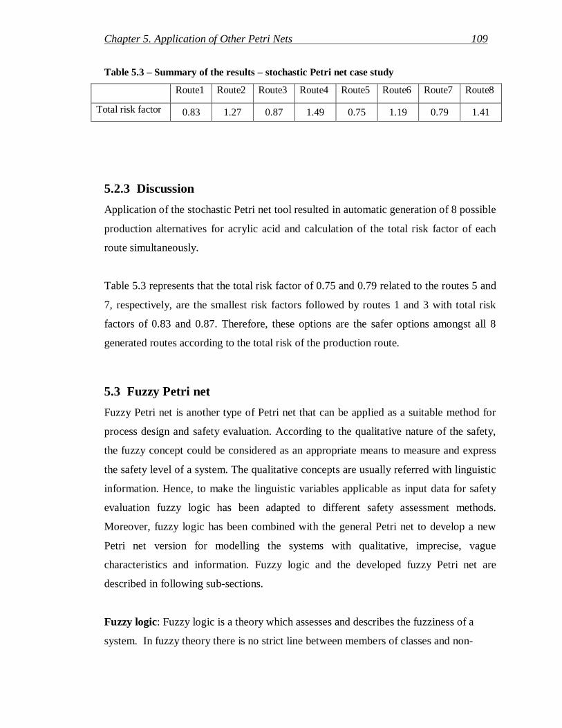
Chapter 5. Application of Other Petri Nets 109
Table 5.3 – Summary of the results – stochastic Petri net case study
Route1 Route2 Route3 Route4 Route5 Route6 Route7 Route8
Total risk factor 0.83 1.27 0.87 1.49 0.75 1.19 0.79 1.41
5.2.3 Discussion
Application of the stochastic Petri net tool resulted in automatic generation of 8 possible
production alternatives for acrylic acid and calculation of the total risk factor of each
route simultaneously.
Table 5.3 represents that the total risk factor of 0.75 and 0.79 related to the routes 5 and
7, respectively, are the smallest risk factors followed by routes 1 and 3 with total risk
factors of 0.83 and 0.87. Therefore, these options are the safer options amongst all 8
generated routes according to the total risk of the production route.
5.3 Fuzzy Petri net
Fuzzy Petri net is another type of Petri net that can be applied as a suitable method for
process design and safety evaluation. According to the qualitative nature of the safety,
the fuzzy concept could be considered as an appropriate means to measure and express
the safety level of a system. The qualitative concepts are usually referred with linguistic
information. Hence, to make the linguistic variables applicable as input data for safety
evaluation fuzzy logic has been adapted to different safety assessment methods.
Moreover, fuzzy logic has been combined with the general Petri net to develop a new
Petri net version for modelling the systems with qualitative, imprecise, vague
characteristics and information. Fuzzy logic and the developed fuzzy Petri net are
described in following sub-sections.
Fuzzy logic: Fuzzy logic is a theory which assesses and describes the fuzziness of a
system. In fuzzy theory there is no strict line between members of classes and non-

Chapter 5. Application of Other Petri Nets 110
members. In other words, everything owns a degree of membership in one or more
classes. This theory was introduced by logician and philosopher Lukasiewicz in the
1930s and rediscovered and adapted for mathematical application by Lotfi-Zadeh in
1965.
Fuzzy logic is a set of rules which defines the degree of membership instead of crisp
membership which is used in conventional binary logic. In binary logic a value may be
false or true which is parallel to 0 or 1 however in fuzzy logic a value may be partly true
and partly false. This degree of membership is expressed through a real number in the
interval [0, 1] (Negnevitsky, 2002).
Fuzzy logic or fuzzy set theory also known as possibility theory may be confused with
probability theory. The first one defines the degree of membership in a set while the
second one shows the likelihood of an element to be in that set. The variables in fuzzy
logic are linguistic variables which are divided into some fuzzy sets. The overlap of a
fuzzy set with other fuzzy sets is the most important point in the fuzzy set theory which
explains how a member can belong to more than one class at the same time. The
membership value shows the degree of belonging into a particular class (Gentile et al.,
2003).
By not using crisp data the fuzzy logic is a proper approach to deal with systems which
have a high level of uncertainty. Many engineering systems are known as systems which
work based on uncertain, qualitative values and subjective knowledge such as expert
systems, control systems and safety and risk modelling systems (Negnevitsky, 2002; Sii
et al., 2001).
Mathematical definition – fuzzy sets: A fuzzy set is a set with fuzzy boundaries. If X is
the universe of discourse and x is its element, in traditional crisp set definition the
characteristic function of A is fA(x);
fA(x) : X → 0, 1,
Where

Chapter 5. Application of Other Petri Nets 111
fA(x) =
The traditional set is a two-element set which is equal to 1 if the x is an element of X and
equal to 0 if x is not an element of X.
However, in fuzzy set theory, the membership function of µA(x) defines fuzzy set A of
universe X in which;
µA(x) : X → [0, 1],
Where
µA(x) = 1 if x is totally in A;
µA(x) = 0 if x is not in A;
0 < µA(x) < 1 if x is partly in A.
In a fuzzy set, the value of membership function shows the degree to which x is a
member of set A. It can be a value in the interval [0, 1] (Negnevitsky, 2002). As
mentioned earlier fuzzy sets may overlap with their nearest fuzzy sets so that a variable
can belong to more than one fuzzy set at the same time with different a membership
degree. Figure 5.1 gives a graphical demonstration of this fact.
Variable (for example, Risk)
0
1Low Medium High
Figure 5.1 – Graphical representation of the fuzzy sets

Chapter 5. Application of Other Petri Nets 112
Fuzzy rule-based systems: The degree of membership allows fuzzy reasoning to deal
with approximate rather than precise reasoning. Fuzzy logic, using fuzzy rules, provides
the possibility to convert subjective human reasoning into Boolean based machine logic.
Moreover, human expertise and knowledge can be represented in the form of fuzzy
rules. Fuzzy logic usually uses IF-THEN rules or any equivalent options. The general
format of a single rule is:
if x is A then y is B
in which x and y are linguistic values defined by the fuzzy set on universes of A and B,
respectively (Xu et al., 2002). Each rule has two fuzzy propositions: an antecedent, if x
is A, which is compared to input and a consequent that is the result, then y is B. The
antecedent must be true before the consequence can be claimed (Bowles & Pelaez,
1995). Any of the propositions in a fuzzy rule may be atomic or compound.
Fuzzy rules are generated by experts or extracted from statistical data (Mendel, 1995).
Some examples of these rules are: in a unit operation, if failure rate is High AND
severity of the consequences is Low then the condition is Unsafe; if failure rate is
Medium AND severity of consequences is Ignorable then the condition is Very safe; if
failure rate is Very high AND severity of consequences is High then the condition is
Extremely unsafe.
A fuzzy rule may have multiple antecedents which are combined together with the
appropriate fuzzy operators such as AND or OR. Different parts of the antecedents are
evaluated simultaneously and resoled to a single number based on the defined fuzzy sets
and applied fuzzy operators. The output of each fuzzy rule is a fuzzy set; however, the
output of a fuzzy system need to be a single number.
A two-step process has to be undertaken to achieve a single crisp output using a fuzzy
system. In the first step, the fuzzy system aggregates all output fuzzy sets into a single
fuzzy set. In the next step, the obtained fuzzy set has to be defuzzified to give a single
number.

Chapter 5. Application of Other Petri Nets 113
The whole process of mapping from a given crisp input to obtaining a single crisp
output is referred to as a fuzzy inference. Several fuzzy inferences are reported in the
literature such as Mamdani-style and Sugeno-style inferences (Mendel, 1995;
Negnevitsky, 2002). The Mamdani-style inference is the most widely used technique;
however, it is not computationally efficient. Sugeno (1985) slightly modified this
method and introduced the Sugeno-style technique which is much easier to apply and
contains less intense computations.
The entire process of the Sugeno-style fuzzy inference is completed in four steps:
fuzzification of the input variables, rule evaluation, aggregation of the rule consequents,
and defuzzification. These four steps are illustrated in Figure 5.2 through a simple two-
input one-output problem including three rules as follows.
In this problem x, y and z are linguistic variables; A1, A2 and A3 are linguistic values
determined by fuzzy sets on universe of X; B1 and B2 are linguistic values determined
by fuzzy sets on universe of Y; C1, C2 and C3 are linguistic values determined by fuzzy
sets on universe of Z.
In this method, the output of each fuzzy rule is constant that is, the membership
functions of the consequents are defined as singleton spikes. As is illustrated in Figure
5.2 all these singletons are taken into account through the aggregation process. The final
crisp output is calculated as the weighted average of these singletons in the Sugeno-style
inference. In the example given in Figure 5.2 the crisp output is obtained through the
following calculation:
Weighted average = ( M(k1) × k1 + M(k2) × k2 + M(k3) × k3 ) / ( M(k1) + M(k2) +
M(k3) )

Chapter 5. Application of Other Petri Nets 114
OR(max)
AND(min)
0.6
0.2
0
1 1
0.8
0.2
0x1 y1
x1 y10
1
0.0
1
0.2 0.2
1
k10 0X Y
YX
X
X
Z
Z
Z
ZZZZ
Z
k2
k3
k1 k2 k3
z1
k3k2k1
x1
x1
y1 Y
0.2
0.8
0.2
0.6
0.20.2
0.6 0.6
0.2
1 1 1
1 1
1 1 1 1
0 0 0
0 0
0 0 0 0
0
Crisp input x1 Crisp input y1
A1
A2
A3B1 B2
A3 B1
A2 B2
A1
M(x=A1)=0.6
M(x=A2)=0.2
M(y=B1)=0.8
M(y=B2)=0.2
Fuzzification
Rule evaluation
Rule 1: IF x is A3 (0.0) OR y is B1(0.2) THEN z is k1(0.2)
Rule 2: IF x is A2 (0.2) OR y is B2(0.8) THEN z is k2(0.2)
Rule 3: IF x is A1 (0.6) THEN z is k3(0.6)
Aggregation of rule consequents
z is k1(0.2) z is k2 (0.2) z is k3 (0.6) aggregation
Defuzzification
Crisp output z1
Figure 5.2 – Sugeno-style fuzzy inference

Chapter 5. Application of Other Petri Nets 115
5.3.1 Fuzzy set theory and safety assessment
Safety and risk analysis is an engineering area which widely deals with imprecise
information. Moreover, when safety analysis results are required as input data for the
decision making phase in the early design stages, these analyses should be conducted
based on very uncertain and vague data which are available at that stage.
Quantitative or semi-quantitative safety assessment methods force designers to measure
the linguistic variables they usually use within a quantitative scale. Qualitative methods
also need to be quantified through specific methods and indexing systems which are
usually based on crisp data and involve strict and crisp boundaries. These types of
quantification methods introduce the additional uncertainty into safety data and decrease
their accuracy.
Uncertainty associated with safety data may be the result of their fuzziness or
randomness therefore fuzzy theory is an appropriate method that can be applied in this
area. This method is well suited to deal with uncertain data and is an efficient way to
smooth down the strict boundaries. With the aid of fuzzy variables it is possible to
express expert estimates and describe uncertain inputs due to fuzzy variables‟ potential
to approximately reflect the available data and finely portray the uncertainty (Cooper,
1994).
Several researches have been carried out to develop an applicable and proper framework
to integrate fuzzy logic into either safety evaluation methods or implementation tools to
achieve above mentioned enhancements. In some studies possibility theory which is the
other name for fuzzy set theory is used instead of traditional probability theory in order
to take into account the uncertainty associated with the failure rate data, the severity of
the consequences and detection of failure (Moller et al., 1999).
Some researches have developed a fuzzy logic framework to deal with natural language
used in expressing safety information and experts‟ opinions such as Failure Modes and
Effects Analysis (FMEA) information and also vagueness of available data. The

Chapter 5. Application of Other Petri Nets 116
potential of fuzzy logic in combining and reflecting the qualitative relation between
failures and modes is of great importance in these type of methods (Bowles & Pelaez,
1995; Xu et al., 2002).
The other category of safety assessment methods which takes advantage of the fuzzy set
theory, includes index based methods. In traditional indexing systems which are based
on Boolean mathematics and intervals with sharp boundaries a small change in a
parameter‟s value may cause a sudden change in the value of the related index. The
ability of fuzzy sets and membership function in converting the crisp boundaries into
fuzzy boundaries causes significant improvement in the accuracy of the results of these
systems. Fuzzy logic introduces a smooth transition from one interval to another and
also because of the possibility of multiple memberships, this approach may provide a
more accurate analysis of uncertain data (Gentile et al., 2003).
The above-mentioned approaches are some examples of the application of fuzzy set
analysis in safety and risk evaluation techniques and methods. In earlier sections of this
study Petri net has been introduced as a proper safety evaluation and process modelling
tool which has the capability of carrying out different qualitative and quantitative as
well as index based safety assessment methods. In the following sections high-level
fuzzy Petri net is described briefly and some modifications are done to develop a
suitable tool to fulfil the purpose of this study. The performance of the proposed tool is
demonstrated by revisiting the acrylic acid case study.
5.3.2 Fuzzy set theory and Petri net modelling
Petri net has been considered as a suitable alternative to represent rules in knowledge-
based systems in the literature. Petri net has the ability to create a well structured
representation of the knowledge-based systems and clearly shows the relation between
the rules.

Chapter 5. Application of Other Petri Nets 117
Much research have been done to develop different formulation methods for fuzzy Petri
net (Scarpelli et al., 1996; Srinivasan & Gracanin, 1993).
In this study a high-level fuzzy Petri net is adopted to model fuzzy reasoning risk
analysis systems which is described as follows:
In the high-level Petri net transitions and places represent the input linguistic variables
and fuzzy sets related to unit operations‟ failure rates and severity of the consequences
of the failures, respectively. The output linguistic variable which is the safety condition
is signified by tokens. The membership values of the variables in the fuzzy sets are
calculated using the proper equations defined in the Petri net model. The arcs connecting
transitions and places perform fuzzy rules between different fuzzy sets and fuzzy
variables. The mathematical definitions are as follows and Figure 5.3 illustrates this
Petri net model:
In each place pi P the fuzzy sets of S = {s1, s2, s3, …, sm} show the severity of the
consequences.
In each transition tj T the fuzzy sets of F = {f1, f2, f3, …, fk} show the failure rate of the
unit operation.
Each token in a place p P shows the fuzzy set C = {c1, c2, c3, …, cl} representing the
safety condition of respective unit operation
Where
i = 1, …, n is the number of unit operation;
j = 1, …, n is the number of start points related to unit operations;
m is the number of fuzzy sets showing the severity of the consequences;
k is the number of fuzzy sets showing the failure rate of the unit operations;
l is the number of fuzzy sets representing the safety condition of each unit operation.
Firing rules are the same as general firing rules applied in general Petri net. A transition
is called enabled if all its input places contain required tokens. During the firing process

Chapter 5. Application of Other Petri Nets 118
the tokens may be removed from the input place to the output place through the
connecting arc. This arc applies the defined fuzzy rules between start transition and
following place and calculates the fuzzy value of the safety condition related to the unit
operation. The fuzzy results of all rules evaluation are aggregated into a unique fuzzy
value. This fuzzy value is changed to crisp value through a difuzzification process and
the final value is transferred to the next unit operation by the tokens. The summation of
all defuzzified safety condition values gives the unique risk factor of each process
option at the end of the modelling process (Pedrycz & Gomide, 1994; Scarpelli et al.,
1996).
FS
p1 p2
Fuzzy rules
t1
C
Figure 5.3 – Graphical representation of a Fuzzy Petri net
5.3.3 Case study
The performance of a fuzzy safety assessment system using fuzzy Petri net is shown in
acrylic acid case study adapted earlier in this project. This fuzzy safety assessment
system is based on the probabilistic risk analysis method. According to the uncertainty
associated with the input data in the probabilistic risk analysis method, fuzzification of
these data can be considered a suitable solution to deal with this issue. The fuzzy risk
analysis method provides the opportunity for the application of the linguistic variables
instead of numerical variables. The four steps of developing a fuzzy risk analysis
inference are described as follows (Negnevitsky, 2002):
Definition of the linguistic variables: in this step the input and output variables and
their ranges need to be determined. In this case study three main linguistic variables are

Chapter 5. Application of Other Petri Nets 119
required including two input variables and one output variable. The “Failure Rate” and
“Severity Of The Consequences” are the input variables defined for transitions showing
the start of operations and places representing the unit operations, respectively. The
“Safety Condition” is the output variable which is carried by tokens in the fuzzy Petri
net. Each of the input variables are described by five fuzzy sets: ignorable; low;
medium; high; and very high. The interactions of these two variables are described by
fuzzy rules which are represented on the connecting arcs in the fuzzy Petri net and result
in production of the knowledge on the variable “Safety Condition” showing the output
which is also described by five fuzzy sets of: extremely unsafe; very unsafe; unsafe;
safe; and very safe.
The respective numerical ranges assigned to linguistic variables are given in Tables 5.4,
5.5 and 5.6. These ranges are obtained using the same data sources as in the probabilistic
case study in section 5.2.2. The intervals are adjusted to be within the range of [0, 1] by
dividing by 10 in the case of the severity of the consequences data.
Table 5.4 – Linguistic variable of Failure Rate
Linguistic variable: Failure Rate
Linguistic value Very low Low Medium High Very high
Numerical range [0, 0.1] [0.05, 0.15] [0.1, 0.25] [0.2, 0.4] [0.3, 1]
Table 5.5 – Linguistic variable of Severity of the Consequences
Linguistic variable: Severity Of The Consequences
Linguistic value Very low Low Medium High Very high
Numerical range [0, 0.1] [0, 0.3] [0.2, 0.4] [0.35, 0.6] [0.5, 1]

Chapter 5. Application of Other Petri Nets 120
Table 5.6 – Linguistic variable of Safety Condition
Linguistic variable: Safety Condition
Linguistic value Extremely unsafe Very unsafe Unsafe Safe Very safe
Numerical range [0, 0.1] [0.05, 0.25] [0.1, 0.3] [0.25, 0.5] [0.3, 1]
Singleton spike 0.05 0.15 0.20 0.42 0.45
Determination of the fuzzy sets: in the second step, the shape of each fuzzy set should
be determined. Amongst the variety of shapes that fuzzy sets may have a triangle or a
trapezoid can adequately represent the experts‟ opinions. Moreover, application of each
of these shapes simplifies the computation to a great extent.
The fuzzy sets for all three variables are shown in Figures 5.2, 5.5 and 5.6. To obtain
smooth response, it is important to provide sufficient overlaps in adjacent fuzzy sets.
Different resources suggest that an overlap between 25 and 50 percent of the bases is
suitable for the triangle-to-triangle and trapezoid-to-triangle fuzzy sets (Negnevitsky,
2002).
Failure Rate
0
1
Low Medium High Very highVery low
0.1 0.2 0.3 0.4
Figure 5.4 – Fuzzy sets related to the Failure Rate variable

Chapter 5. Application of Other Petri Nets 121
Severity Of The Consequences
0
1
Low Medium HighVery low Very high
0.1 0.2 0.3 0.4 0.5 0.6
Figure 5.5 – Fuzzy sets related to the Severity of the Consequences variable
Safety Condition
0
1
Extremely
unsafe
Very
unsafe Unsafe Safe Very safe
0.1 0.3 0.50.2 0.4
Figure 5.6 – Fuzzy sets related to the Safety Condition variable
Construction of fuzzy rules: in this step the fuzzy rules have to be formed. For this
purpose an expert may be asked to describe the system behaviour based on the defined
linguistic variables and their linguistic values. In the developed fuzzy Petri net model
the fuzzy rules are assigned to the arcs connecting the start transitions to the unit
operation places.
For a three-variable system the fuzzy rules may be presented in a two-dimension matrix.
The vertical and horizontal axes show the values of input variables and the intersections

Chapter 5. Application of Other Petri Nets 122
of rows and columns give the values of output variable. Table 5.7 shows the rule matrix
created for this case study.
Table 5.7 – Matrix of fuzzy rules
Severity of the consequences
Failure rate Ignorable Low Medium High Very high
Very low Very safe Very safe Safe Safe Safe
Low Very safe Very safe Safe Unsafe Unsafe
Medium Very safe Safe Unsafe Unsafe Very unsafe
High Safe Unsafe Very unsafe Very unsafe Ext unsafe
Very high Unsafe Unsafe Very unsafe Ext unsafe Ext unsafe
Twenty five fuzzy rules can be obtained from this table which are described in Table
5.8.
Table 5.8 – Fuzzy rules
Rule
No.
Antecedent Consequent
1 IF Failure rate = Very low AND Severity of the
consequences = Ignorable
THEN Condition = Very
safe
2 IF Failure rate = Very low AND Severity of the
consequences = Low
THEN Condition = Very
safe
3 IF Failure rate = Very low AND Severity of the
consequences = Medium
THEN Condition = Safe
4 IF Failure rate = Very low AND Severity of the
consequences = High
THEN Condition = Safe
5 IF Failure rate = Very low AND Severity of the
consequences = Very high
THEN Condition = Safe

Chapter 5. Application of Other Petri Nets 123
Rule
No.
Antecedent Consequent
6 IF Failure rate = Low AND Severity of the
consequences = Ignorable
THEN Condition = Very
safe
7 IF Failure rate = Low AND Severity of the
consequences = Low
THEN Condition = Very
safe
8 IF Failure rate = Low AND Severity of the
consequences = Medium
THEN Condition = Safe
9 IF Failure rate = Low AND Severity of the
consequences = High
THEN Condition = Unsafe
10 IF Failure rate = Low AND Severity of the
consequences = Very high
THEN Condition = Unsafe
11 IF Failure rate = Medium AND Severity of the
consequences = Ignorable
THEN Condition = Very
safe
12 IF Failure rate = Medium AND Severity of the
consequences = Low
THEN Condition = Safe
13 IF Failure rate = Medium AND Severity of the
consequences = Medium
THEN Condition = Unsafe
14 IF Failure rate = Medium AND Severity of the
consequences = High
THEN Condition = Unsafe
15 IF Failure rate = Medium AND Severity of the
consequences = Very high
THEN Condition = Very
unsafe
16 IF Failure rate = High AND Severity of the
consequences = Ignorable
THEN Condition = Safe
17 IF Failure rate = High AND Severity of the
consequences = Low
THEN Condition = Unsafe
18 IF Failure rate = Medium AND Severity of the
consequences = Medium
THEN Condition = Very
unsafe
19 IF Failure rate = High AND Severity of the
consequences = High
THEN Condition = Very
unsafe

Chapter 5. Application of Other Petri Nets 124
Rule
No.
Antecedent Consequent
20 IF Failure rate = High AND Severity of the
consequences = Very high
THEN Condition =
Extremely unsafe
21 IF Failure rate = Very high AND Severity of
the consequences = Ignorable
THEN Condition = Unsafe
22 IF Failure rate = Very high AND Severity of
the consequences = Low
THEN Condition = Unsafe
23 IF Failure rate = Very high AND Severity of
the consequences = Medium
THEN Condition = Very
unsafe
24 IF Failure rate = Very high AND Severity of
the consequences = High
THEN Condition =
Extremely unsafe
25 IF Failure rate = Very high AND Severity of
the consequences = Very high
THEN Condition =
Extremely unsafe
Implication of the fuzzy system: next the fuzzy sets and fuzzy rules have to be encoded
using an available fuzzy logic development tool or a programming language such as
C++. The C++ programming language is applied in this project to develop the fuzzy
system. The developed codes are available in Appendix B.
Once the fuzzy inference has been developed the crisp data previously applied in the
same case study in Section 5.2.2 are used as the input data in this system.
5.3.4 Discussion
The same as previous applications of this case study using the Petri net tool, the fuzzy
approach also results in automatic generation of 8 possible routes. Table 5.9 shows that
using the fuzzy risk analysis method, the total risk factors calculated for these 8
production options are between 0.1 and 0.25. The overall results in this method are

Chapter 5. Application of Other Petri Nets 125
almost the same as the results obtained using the probabilistic risk analysis method and
stochastic Petri net tool. However, some minor differences are observed which might be
due to the impacts of fuzzification and the use of the smooth boundaries instead of sharp
boundaries and crisp data.
Three different groups are distinguished according to the obtained results. In the first
group, including routes 1, 3, 5 and 7, the final risk factor value is 0.1. In the second and
third groups, the calculated values for the final factor are 0.20 and 0.25, respectively.
The unity of the final risk factor values of all alternatives in one group is a result of
smoothing specification of the fuzzy approach. Amongst the detected groups, the first
one contains the safest process options with the lowest fuzzy risk factor of 0.1.
Table 5.9 – Summary of the results - fuzzy Petri net case study
Route1 Route2 Route3 Route4 Route5 Route6 Route7 Route8
Total risk factor 0.10 0.25 0.10 0.20 0.10 0.25 0.10 0.20
5.4 Conclusion
The stochastic Petri net and fuzzy Petri net have been introduced briefly and their
capabilities to be applied as implementation tools for executing different safety and risk
analysis methods have been explained. The stochastic Petri net has been applied to
perform the probabilistic risk analysis method and the fuzzy Petri net has been adapted
to carry out the fuzzy risk analysis. The efficiency of their performances has been
demonstrated through the acrylic acid case study.
The flexibility of the Petri net tool to be adapted and applied in variety of situations and
systems in addition to the compatibility of different types of Petri nets with various
safety and risk evaluation methods have been outlined in this chapter. These
characteristics plus the capability of this tool to be applied at any level of a plant life-
cycle further proves the suitability of Petri nets for the purposes of this study.

Chapter 5. Application of Other Petri Nets 126
References
Bowles, J. B., & Pelaez, C. E. (1995). Fuzzy logic prioritization of failures in a system
failure Bowles, J. B., & Pelaez, C. E. (1995). Fuzzy logic prioritization of
failures in a system failure mode, effects and criticality analysis. Process Safety
Progress, 50(2), 203-213.
Ciardo, G., German, R., & Lindemann, C. (1994). A characterization of the stochastic
process underlying a stochastic Petri net. IEEE Transactions on software
engineering, 20(7), 506-515.
Cooper, J. A. (1994). Fuzzy-algebra uncertainty analysis for abnormal-environment
safety assessment (No. SAND93-2665.UC-706). New Mexico: Sandia National
Laboratories.
Gentile, M., Rogers, W. J., & Mannan, M. S. (2003). Development of an inherent safety
index based on fuzzy logic. AIChE Journal, 49(4), 959-968.
Jiang, Z., Zuo, M. J., & Fung, R. Y. K. (1999). Stochastic object-oriented Petri nets
(SOPNs) for reliability modeling of manufacturing systems. Paper presented at
the Proceeding of the 1999 IEEE Canadian Conference on Electrical and
Computer Engineering Edmonton, Alta., Canada.
Lees, F. P. (1996). Loss prevention in the process industries: hazard identification,
assessment, and control (2nd ed.): Elsevier Butterworth-Heinemann.
Mendel, J. M. (1995). Fuzzy logic systems for engineering: a Tutorial. Proceedings of
the IEEE, 83(3), 345-377.
Moller, B., Beer, M., Graf, W., & Hoffmann, A. (1999). Possibility theory based safety
assessment. Computer and Infrastructure Engineering, 14(2), 81-91.
Negnevitsky, M. (2002). Artificial intelligence: a guide to intelligent systems (first ed.
Vol. 1): Pearson Education Limited.
Parzen, E. (1999). Stochastic processes: SIAM.
Pedrycz, W., & Gomide, F. (1994). Ageneralized fuzzy Petri net model. IEEE
Transactions on Fuzzy systems, 2(4), 295-301.
Scarpelli, H., Gomide, F., & Yager, R. (1996). A reasoning algorithm for high-level
fuzzy Petri nets. IEEE Transactions on Fuzzy systems, 4(3), 282-294.
Sii, H. S., Ruxton, T., & Wang, J. (2001). A fuzzy-logic-based approach to qualitative
safety modelling for marine systems. Reliability Engineering & System Safety,
73(1), 19-34.
Srinivasan, P., & Gracanin, D. (1993). Approximate reasoning with fuzzy Petri nets.
Paper presented at the Second IEEE International Conference on Fuzzy Systems.
Xu, k., Tang, L. C., Xie, M., Ho, S. L., & Zhu, M. L. (2002). Fuzzy assessment of
FMEA for engine systems. Reliability Engineering & System Safety, 72(1), 17-
29.
Zhou, M. C., DiCesare, F., & Guo, D. (1990). Modeling and performance analysis of a
resource-sharing manufacturing system using stochastic Petri nets. Paper
presented at the 5th IEEE International Symposium on Intelligent Control.

Chapter 6. Methodology Development 127
CChhaapptteerr 66
MMeetthhooddoollooggyy DDeevveellooppmmeenntt
6.1 Introduction
The combined Petri net tool proposed in this study aims to provide the possibility of
conducting safety assessment during the initial stages of a process design through
developing an integrated framework. This framework efficiently overcomes the
shortcoming of late safety consideration during the process design and the subsequent
issues pointed out in Chapter 2. The limitation of the safety aspects that can be evaluated
in each of existing method is another important lacking area which makes these
approaches inefficient for conducting a comprehensive safety assessment. A modified
safety and risk assessment method is required to account for wider spectrum of safety
issues to offer an inclusive evaluation of the safety and risk status in a system. Such
safety and risk evaluation method is able to provide a reliable comparison base for
decision-making purposes. Thus, before proceeding with the application of the proposed
implementation tool, a methodology development is proposed in this chapter as a
significant contribution to the available literature. The methodology development is
based on two main safety assessment methods explained in Chapter 2; the inherent
safety assessment method and the probabilistic risk analysis.
The new methodology is described in detail in Section 6.2. The acrylic acid case study is
revisited in Section 6.3 to evaluate the performance of the new methodology. The

Chapter 6. Methodology Development 128
chapter concludes in Section 6.4 by providing a discussion on the applicability of this
methodology and the results.
6.2 New methodology
As mentioned in Chapters 2 and 3, there is increasing interest among industries in safety
assessment methodologies which are applicable in the initial stages of the process design
and are capable of evaluating a wide range of safety aspects concurrently.
The existing methods come under two main groups depending on the nature of the
safety issues that they attempt to evaluate. One major category of methods focuses on
the safety of the process conditions including chemical conditions and physical
conditions, while the other main category emphasises the risk of failure of the unit
operations involved in the process.
Chemical conditions such as toxicity, flammability and explosiveness and physical
conditions such as pressure and temperature are considered as main factors influencing
safety of a process in the first group. Inherent safety assessment is an example of this
group (Heikkila, 1999; Heikkila et al., 1996).
The second group accounts for the reliability level of equipment to start working or
continue to work in different situations. Probabilistic risk assessment, fault tree analysis,
failure mode and effect analysis, and layer of protection analysis come under this
category (Fullwood & Hall, 1988; Hendershot, 2005).
In this study one well developed technique from each group has been chosen for more
detailed investigation based on the ability to intervene in the early stages of design.
Inherent safety assessment can be implemented at any phase of design by using
chemical and physical information of a process available at that particular level.
Probabilistic risk assessment is also another method which can be employed early
during the design process using experts‟ opinions and available databases. These two

Chapter 6. Methodology Development 129
methods have been described in detail in previous chapters. They also have been applied
separately to a case study using the proposed Petri net implementation tool.
In this step of the study, the possibility of combining these methods and developing a
new method to evaluate a wider range of safety and risk aspects is investigated. The
combined method has to be valid and reliable. Moreover, considering the main concern
of this study, the safety assessment method needs to be relatively simple to be easily
understood and applied by industries. For example, using the multiple-criteria decision-
making tool is an alternative method to evaluate more safety factors simultaneously
(Dicdican & Haimes, 2005). However, this method and the similar available options are
not considered as suitable methods for the purpose of this study based on their
complexity level and required calculations. As mentioned earlier, the emphasis of this
project is on developing a safety assessment tool and technique without the need for
special expertise. This characteristic would make the method capable to be used and
shared as a common language by all designers with different professional areas and
various levels of expertise.
6.2.1 Logical development
Sections 2.3.4 and 4.3.3 showed that inherent safety approach using the I2SI indices
aims to evaluate and quantify the inherent safety level of unit operations and the whole
process based on the defined keywords of: simplification, minimization, substitution and
moderation. The final I2SI index is calculated for each unit operation based on a number
of sub-indices evaluating the chemical and physical conditions safety. The greater than
unity index indicates the positive response of the unit operation to the inherent safety
keywords. A function of the all individual I2SIs in a process is usually used to represent
the safety factor of the entire process ( Eq 2.13 ). The greater I2SI and the total index
represents the safer unit operation and process option, respectively.
On the other hand, the probabilistic risk analysis method attempts to measure the risk
level associated with unit operations and the whole process. If the failure rate of unit

Chapter 6. Methodology Development 130
operations and the severity of the consequences are used as the input data, the
probability risk analysis method would indicate the risk factor related to each unit
operation using Eq 2.1. The summation of all individual risk factors is usually used as
the total risk factor of the entire process (Eq 2.2). The smaller the risk factor the safer
the unit operation or the process option.
A rational and valid combination of the factors introduced in the above methods would
form a unique factor that could take into account both process conditions safety and risk
of failure of the process via a unique factor. Comparing these methods show that the
inherent safety index quantifies the safety level of a system while, the risk factor
measures the hazardous characteristic of that system. In other words, the final factors in
these methods operate in opposite directions; the greater factor in the first method
represents the safer option which is desired, while the greater factor in the second
approach indicates more hazardous option which is undesired. A possible solution to
make these two factors unidirectional is to apply the positive amount of the desirable
factors together with the negative amount of the undesirable indices (Eq 6.1). The
summation of these factors gives a general indication of how safe and reliable is a
process in comparison with the other possible options. It should be noted that this
integrated factor may not be a sufficient factor to show the safety level of an individual
process since it is just a numerical index with no specific dimension. However, it
provides a suitable comparison base for decision-making purposes to choose the safer
options amongst all available alternatives considering both safety and reliability
characteristics.
Total safety factor = ( + total I2SI index ) + ( – total risk factor ) (Eq 6.1)
6.2.2 Mathematical development
Based on the above-mentioned logic the inherent safety and risk factors need to be
mathematically combined to obtain a unique index for each process option. To create a

Chapter 6. Methodology Development 131
valid combination these two different factors need to be mathematically compatible in
various aspects.
Firstly, in a mathematical equation to apply addition or subtraction operators between
different components they need to have similar dimensions or be dimensionless. Given
that the I2SI and as a result the total I2SI is a dimensionless component, the other
component which is the risk factor has to be dimensionless as well (Khan & Amyotte,
2005).
To achieve a dimensionless risk factor using Eq 2.1 the only applicable solution is to
make both failure rate and severity of the consequences dimensionless. An appropriate
alternative for the failure rate of a unit operation suggested in the literature to serve this
purpose is the ratio of the number of failures of that unit operation in a certain period of
time to the total number of all failures in the process option during the same period of
time (Eq 6.2). Since both sides of this fraction have the same dimensions, the total
fraction would be dimensionless (Lees, 1996).
The total number of failures in this equation takes into account all possible failures with
different sources that may happen over the defined period of time. A brief review of the
literature revealed that there are some major sources which can be classified as the most
common causes of the hazardous events in the process industries. Following categories
of failure sources are mutually agreed via different researches: plant and equipment,
human, and environmental. The share of each source in creating the hazardous events
mentioned in various researches are not exactly the same; however, plant and equipment
related failures are usually the most frequent failures followed by human errors. The
percentage of the technical failures ranges from 40% to 60% of the total undesired
events in the industries according to the literature (Baranzini & Christou, 2009; Flynn &
Theodore, 2001; Kariuki & Lowe, 2007).
To account for the number of failures caused by different sources other than plant and
equipment, an adjustment factor named 𝜎 is applied in this study for the calculation of

Chapter 6. Methodology Development 132
the unit operations failure rates. The total number of technical failures is multiplied by
this adjustment factor which is always greater than unity to take into account the number
of failures caused by all major sources. The value of the adjustment factor may vary
from one industry to another industry or even one case to another case in the same
industry based on the available historical data and experts‟ opinions.
(Eq 6.2)
Where
i=1,…, n while n is the number of unit operations
t is the time period
𝜎 is the adjustment factor
The indices applied in the previous chapters indicating the severity of the consequences
are also dimensionless. Each of these indices represents a linguistic value which defines
the severity of the consequences of a failure. These linguistic variables and the
respective indices are identified based on the experts‟ opinions and available databases
(Table 5.1).
The second important issue is that the range of the values that inherent safety indices
and risk factors may obtain should be the same or close enough. Since the I2SI index is
a function of a variety of other sub-indices calculated using different databases and
methods, it is not easily possible to make major changes in the range of these
components and meanwhile keep the final index valid. Hence, this index and the
respective sub-indices are applied in this study as they have been proposed in the
original study with no change in the range of their values. The values of two main sub-
indices of ISPI and HI forming the final I2SI index range from 1 to 200 (Khan &
Amyotte, 2004). Since these indices are combined through Eq 2.13, the final index value
varies in the range of [0.005, 200].

Chapter 6. Methodology Development 133
To be compatible with the I2SI the risk factor should be within the same range.
According to the probability theory, Eq 6.2 and also considering the fact that the
numerator of the fraction in this equation is always smaller than the denominator, the
value of the failure rate is always within the range of [0, 1]. Hence, the range of the
severity of the consequences which is the other component of the risk factor has to be
modified to meet this criterion. This factor is quantified subjectively based on experts‟
opinions and divided in nine groups listed in Table 5.1. However, these values need to
be normalised between 1 and 200 to be applicable in the proposed combined method.
The linear interpolation method ( Eq 6.3) is applied to construct the points in the range
of [1, 200] respective to the known points in the range of [1, 10]. Table 6.1 gives the
new values representing the severity of the consequences.
y = ya + ( x – xa ) ( yb – ya ) / ( xb – xa ) (Eq 6.3)
Where
xa and xb are lower and upper limits, respectively in given range
ya and yb are lower and upper limits, respectively in new range
x is the known point in given range
y is unknown point in the new range respective to point x

Chapter 6. Methodology Development 134
Table 6.1 – Severity of the Consequences normalised within the range of [1, 200]
Severity of the consequences Normalised Index [1, 200] Rounded Index
Extremely high 200 200
Very high 177.9 178
Not greatly high but noticeable 155.8 156
Noticeable 133.7 134
Moderately noticeable 111.5 111
Reasonable 89.4 89
Low 67.3 67
Significantly low 45.2 45
Ignorable 1…23 1…23
Considering the new severity of the consequences data and the failure rate, the final risk
factor which is a product of these two factors, ranges from 0 to 200 which is almost in
the same range as I2SI factor.
6.2.3 Methodology enhancement
The next step of the methodology development focuses on enhancing the performance
of the combined method by modifying its individual components. A more
comprehensive study on the results of application of the inherent safety method on the
acrylic acid case study elucidates that the total I2SI index calculated for the entire
process route is directly affected by the number of unit operations existing in that route.
This means that an increase in the number of unit operations would definitely increase
the value of the total I2SI regardless of the safety characteristics of the added unit
operations. This issue is due to the mathematical attributes of the Eq 2.12. Considering
this equation, any additional individual I2SI which is always a positive value would
result in a greater total I2SI, no matter whether the added I2SI is less than unity which
indicates the poor safety situation of the related unit operation or is greater than unity
which represents the inherently safe condition of the unit operation. Moreover, using the

Chapter 6. Methodology Development 135
square root in this formula regardless of the number of contributing factors
unnecessarily intensifies the impact of the larger I2SI available in a system on the total
value of I2SI. That is when a unit operation has a relatively noticeable greater I2SI in
comparison with the other unit operations in a process option with more than two unit
operations the large I2SI would have an emphasised impact on the total I2SI of the
route. It happens according to the fact that the degree of the root is always 2 irrespective
of the number of participating units. A modified technique and equation are required to
overcome these problems.
A possible solution which is suggested in this study is to apply the averaging technique
to calculate a final index which indicates the general and normal safety situation of the
process. Two different averaging systems may be applicable in this case: the arithmetic
mean and the geometric mean. These two methods are described briefly and their
mathematical equations are given as follows.
Arithmetic averaging – is the most familiar method of averaging in which the
summation of n factors are divided by n to obtain the norms of n factors (Eq 6.4). Since
the arithmetic mean is a sum-based value, it is appropriate for the additive processes
(Humphries, 2008).
(Eq 6.4)
Where
n is the number of factors (xi).
Geometric averaging – to calculate the geometric mean of n factors they are multiplied
together then the nth root of the product is taken (Eq 6.5). The geometric means are
product-based values which are suitable for multiplicative processes (Humphries, 2008).

Chapter 6. Methodology Development 136
(Eq 6.5)
Where
n is the number of factors (xi).
According to the specification of these averaging techniques and the multiplicative
characteristic of the I2SI index, the geometric mean is more appropriate to be used in
this study. Application of a proper averaging method would diminish the impact of the
number of unit operations contributing in a system on the final value calculated for that
system. In addition, using the nth
root leads to levelling the weight of all n unit
operations of the system on the calculated average factor. This new index is named the
“average I2SIroute” which is given in Eq 6.6.
(Eq 6.6)
Where
i = 1…n indicates the unit operation/equipment and n is the total number of unit
operations/equipment.
To be able to replace the total I2SIroute with the average I2SIroute in Eq 6.1 the second
component of this equation which shows the total risk factor of the route has to be
replaced with a compatible factor. To meet this requirement the average value of all risk
factors related to the unit operations of the production route is applied instead of their
summation. Considering the multiplicative nature of the individual risk factors, the
geometric mean seems to be the appropriate option to represent the average risk value.
Eq 6.7 is applied to calculate this value which is referred as “average riskroute” in this
study.
(Eq 6.7)
Where

Chapter 6. Methodology Development 137
i = 1…n indicates the unit operation/equipment and n is the total number of unit
operations/equipment.
Implementing the above modifications changes Eq 6.1 to Eq 6.8 as given below.
Final safety factor = Average I2SI route – Average Risk route (Eq 6.8)
This new method provides an enhanced measure of the safety level of the systems which
can be used as a decision-making factor in conjunction with the other factors to compare
different possible production alternatives and choose the safest one. The proposed final
index is not directly affected by the number of unit operations existing in the process
options. Hence, an increase in the number of unit operations does not increase the safety
factor which indicates a safer option. On the other hand, the averaging technique does
not also take into account that additional unit operations increase the complexity of the
systems which may result in reduction in safety level. However, this problem can be
overcome by considering the penalty factor introduced earlier in this study. As
explained in Chapter 4 penalty factor indicates the number of unit operations not
responding to the inherent safety keywords (I2SI less than unity). It means if the
additional unit operations have adverse impacts on the safety level of the system the
penalty factor would increase. By considering penalty factor as another decision-making
factor the complexity of process options with larger number of unit operations would
also be taken into account.
Moreover, the new index gives even weights to all components of a system without
emphasising inherently safer unit operations and highlighting their impacts on the final
result. The final safety index ranges from -199.995 to 200 which is a relatively wide
range giving enough flexibility to calculate the factor in different cases. This range is
fixed considering the minimum and maximum possible values of contributing
parameters.

Chapter 6. Methodology Development 138
It should be mentioned again that although the proposed index may provide a sufficient
comparison base for decision-making purposes to choose the safer process option
amongst available alternatives, it is not a proper indicator for safety and risk level of an
individual option. There is no pre-defined range of values indicating the safe or unsafe
areas. Therefore, the final value of this factor for a single process option which is not
supposed to be compared with other options does not provide any reliable information
about the safety level of that process.
To compare different process alternatives using the proposed index, the greater final
safety factors represent the safer options. The range of final values of safety factors may
vary from case to case. In some cases the final factor of all possible routes may get
negative values while, in other cases they may all be positive. Even in a unique case,
some factors might be in the negative range while the others take positive values. The
decision-making process is not influenced by these ranges and the final decision is make
based on the differences between the final value of indices.
6.2.4 Tool enhancement
Previous chapters revealed that the Petri net modelling tool is capable of being
effectively applied as the process modelling and safety assessment implementation tool.
A place weighted Petri net has also been developed and applied to perform the
concurrent process modelling and inherent safety assessment. Moreover, the stochastic
Petri net has been introduced as a suitable option to execute probabilistic risk analysis at
the same time as process design.
In the new methodology developed in this chapter inherent safety assessment and
probabilistic risk analysis are applied as basic methods. Therefore, taking advantages of
the individual abilities of both place weighted Petri net and stochastic Petri net together
would provide an appropriate means with enough flexibility to implement the new
methodology simultaneously with the process design.

Chapter 6. Methodology Development 139
In this study, this combined Petri net tool is called place weighted stochastic Petri net.
The specifications of different nodes in the proposed Petri net are as follows:
Places (Pi) represent unit operations. Each place owns a two-element weight
factor Pi(w1&2) in which w1 holds the I2SI value and w2 holds severity of the
consequences factor related to the unit operation failure.
Transitions (Tj) show the start of operations of the units. These are stochastic
transitions which their firing are governed by the failure rates of unit operations
dedicated to the transitions Tj(f). The same assumption as in previous chapters is
applied here; if a unit operation (Pi) fails to operate with the probability of Ti(f) ,
the repair or replacement is done in zero time and the unit operation would be
back in process and would be ready for use after zero time.
Arcs connect places to the transitions and transitions to the places.
Tokens are raw materials, semi-finished products and final products which
move from the initial place in the Petri net model to the final place via
transitions and arcs illustrating the flow of materials. They also transfer the
safety data throughout the model.
The proposed method and tool are applied and tested in the acrylic acid case study in the
following part of this chapter and the results are discussed subsequently.
6.3 Application of the new methodology on the acrylic acid case study
Following the application of the acrylic acid case study in Chapter 3 and 4, this case
study is applied in this chapter to evaluate the performance of the proposed method. As
mentioned earlier, in this chapter the proposed method is based on two well-defined
safety assessment approaches of inherent safety and probabilistic risk analysis.

Chapter 6. Methodology Development 140
6.3.1 Implementation and results
The input data related to the inherent safety method is the same as data previously
provided in Table 4.4. The basic data related to the probabilistic risk analysis is also the
same as data given in Table 5.2. However, some modifications are required to make this
data applicable in the new proposed method.
The failure rate and severity of the consequences are two groups of data used in the
probabilistic risk analysis method which both need to be modified to be compatible with
the inherent safety data. First of all, the probability of the failures has to be changed to a
dimensionless factor. To serve this purpose, Eq 6.2 is applied with assuming an average
value of 𝜎 = 2 for the adjustment factor which means the share of the technical failures
is 50% of the total likely failures. Moreover, the indices indicating the severity of the
consequences in chapter 4 have to be adjusted to the new range of [1, 200] using Table
6.1. The modified input data associated with all unit operations for probability risk
analysis purpose is given in Table 6.2.
The proposed methodology is implemented on this case study using the introduced
combined Petri net tool and abovementioned input data. The information related to the
places and transitions are given in Table 6.3. Eqs 6.6, 6.7, and 6.8 are defined in the
Petri net model for safety assessment calculations. The safety information calculated
using the Pi (w1 & 2) and Tj(f) input data in each step is transferred to the next step by the
tokens. The model is run in Visual Studio environment using C++ programming
language. The C++ codes and related explanation is given in Appendix B. Table 6.4
presents the final results of running the Petri net model.

Chapter 6. Methodology Development 141
Table 6.2 – Modified input data related to the unit operations in PRA method
Unit operation Number of failures Failure rate Severity of the consequences
Air compressor 10 0.13 1
Feed mixer 5 0.06 45
Quench tower 3 0.04 23
Reactor 1 0.01 67
Off-gas absorber 3 0.04 67
Solvent splitter 3 0.04 23
Dist. columnI 3 0.04 45
Dist. columnII 3 0.04 1
Dist. columnIII 3 0.04 23
Solvent mixer 3 0.04 1
Extraction tower 3 0.04 45
Table 6.3 – Places’ weight factors and transitions’ firing rates
(a) Route 1
Unit operation Pi Pi (w1) Pi (w2) Tj Tj(f)
Air compressor
Feed mixer
Reactor
Quench tower
Off-gas absorber
Dist. ColumnI
Dist. ColumnII
Dist. ColumnIII
P2
P6
P8
P7
P10
P17
P18
P19
1.39
0.34
0.21
2.50
2.19
0.45
0.49
0.39
1
45
67
23
67
45
1
23
T1
T3
T5
T4
T6
T7
T24
T24
0.13
0.06
0.01
0.04
0.04
0.04
0.04
0.04

Chapter 6. Methodology Development 142
(b) Route 2
Unit operation Pi Pi (w1) Pi (w2) Tj Tj(f)
Air compressor
Feed mixer
Reactor
Quench tower
Off-gas absorber
Solvent splitter
Dist. ColumnI
Dist. ColumnII
Dist. ColumnIII
P2
P6
P8
P7
P10
P15
P17
P18
P19
1.39
0.34
0.21
2.50
2.19
1.05
0.45
0.49
0.39
1
45
67
23
67
23
45
1
23
T1
T3
T5
T4
T6
T8
T8
T24
T24
0.13
0.06
0.01
0.04
0.04
0.04
0.04
0.04
0.04
(c) Route 3
Unit operation Pi Pi (w1) Pi (w2) Tj Tj(f)
Air compressor
Feed mixer
Reactor
Quench tower
Off-gas absorber
Extraction tower
Solvent mixer
Dist. ColumnI
Dist. ColumnII
Dist. ColumnIII
P2
P6
P8
P7
P10
P24
P30
P25
P26
P29
1.39
0.34
0.21
2.50
2.19
3.48
1.41
4.64
2.70
2.04
1
45
67
23
67
45
23
45
1
23
T1
T3
T5
T4
T6
T9
T19&21
T18
T19
T18
0.13
0.06
0.01
0.04
0.04
0.04
0.04
0.04
0.04
0.04

Chapter 6. Methodology Development 143
(d) Route 4
Unit operation Pi Pi (w1) Pi (w2) Tj Tj(f)
Air compressor
Feed mixer
Reactor
Quench tower
Off-gas absorber
Solvent splitter
Extraction tower
Solvent mixer
Dist. ColumnI
Dist. ColumnII
Dist. ColumnIII
P2
P6
P8
P7
P10
P15
P24
P30
P25
P26
P29
1.39
0.34
0.21
2.50
2.19
1.05
3.13
1.44
4.71
2.87
2.10
1
45
67
23
67
23
45
23
45
1
23
T1
T3
T5
T4
T6
T10
T10
T19&21
T18
T19
T18
0.13
0.06
0.01
0.04
0.04
0.04
0.04
0.04
0.04
0.04
0.04
(e) Route 5
Unit operation Pi Pi (w1) Pi (w2) Tj Tj(f)
Air compressor
Feed mixer
Reactor
Off-gas absorber
Dist. ColumnI
Dist. ColumnII
Dist. ColumnIII
P2
P6
P11
P13
P17
P18
P19
1.39
0.34
0.21
0.33
0.45
0.49
0.39
1
45
67
67
45
1
23
T1
T3
T11
T12
T13
T24
T24
0.13
0.06
0.01
0.04
0.04
0.04
0.04

Chapter 6. Methodology Development 144
(f) Route 6
Unit operation Pi Pi (w1) Pi (w2) Tj Tj(f)
Air compressor
Feed mixer
Reactor
Off-gas absorber
Solvent splitter
Dist. ColumnI
Dist. ColumnII
Dist. ColumnIII
P2
P6
P11
P13
P15
P17
P18
P19
1.39
0.34
0.21
0.33
1.05
0.45
0.49
0.39
1
45
67
67
23
45
1
23
T1
T3
T11
T12
T14
T14
T24
T24
0.13
0.06
0.01
0.04
0.04
0.04
0.04
0.04
(g) Route 7.
Unit operation Pi Pi (w1) Pi (w2) Tj Tj(f)
Air compressor
Feed mixer
Reactor
Off-gas absorber
Extraction tower
Solvent mixer
Dist. ColumnI
Dist. ColumnII
Dist. ColumnIII
P2
P6
P11
P13
P24
P30
P25
P26
P29
1.39
0.34
0.21
0.33
3.48
1.41
4.64
2.70
2.04
1
45
67
67
45
23
45
1
23
T1
T3
T11
T12
T15
T19&21
T18
T19
T18
0.13
0.06
0.01
0.04
0.04
0.04
0.04
0.04
0.04

Chapter 6. Methodology Development 145
(h) Route 8
Unit operation Pi Pi (w1) Pi (w2) Tj Tj(f)
Air compressor
Feed mixer
Reactor
Off-gas absorber
Solvent splitter
Extraction tower
Solvent mixer
Dist. ColumnI
Dist. ColumnII
Dist. ColumnIII
P2
P6
P11
P13
P15
P24
P30
P25
P26
P29
1.39
0.34
0.21
0.33
1.05
3.48
1.44
4.71
2.87
2.10
1
45
67
67
23
45
23
45
1
23
T1
T3
T11
T12
T16
T16
T19&21
T18
T19
T18
0.13
0.06
0.01
0.04
0.04
0.04
0.04
0.04
0.04
0.04
Table 6.4 – Summary of the results – new methodology
6.3.2 Discussion
In Table 6.4 the routes with a greater average safety index are considered the safer
options. The penalty factor which is the number of non-responding unit operations to the
application of the inherent safety keywords are also presented in this table. Two safest
options using the new approach are routes 3 and 4 with decision-making factors of
(0.76, 2) and (0.68, 2), respectively. Comparing these factors shows that route 3 is the
Route1 Route2 Route3 Route4 Route5 Route6 Route7 Route8
Average
safety index 0.02 0.03 0.76 0.68 -0.20 -0.18 0.35 0.32
Penalty
factor
5
5
2
2
6
6
3
3

Chapter 6. Methodology Development 146
optimal case with greater average safety index. Route 5 with the decision-making factor
of (-0.20, 6) is the worst process option based on the new method.
The final results of applying the proposed method are slightly different from the
outcomes of the application of the original I2SI system. Two safer options are the same
in both methods; however, the best route is different. It can be explained as a result of
considering more safety factors in the new method compared to the I2SI technique. The
process route 4 including all additional safety features, is the best option according to
the original I2SI; while, considering risk factors as a part of the safety assessment
process in the new method results in altering the safest route from number 4 to the
number 3 which contains fewer additional inherent safety features. This means that the
extra inherent safety feature may increase the inherent safeness of the process; however,
it also increases the risk of failure of the production route. The adverse impact of
including an extra unit operation in this process in terms of increasing the total risk
factor is greater than the inherent safety benefit that this unit operation may introduce to
the process option. Hence, taking into account a wider range of safety factors through
the proposed method changes the final result of the safety evaluation in this case study
compared to the original method.
6.4 Conclusion
This chapter has introduced a methodology for providing adequate decision-making
factors to help with comparing various process alternatives according to their safety
level and choosing the optimal case. The proposed methodology is based on two
efficient assessment methods of the inherent safety approach and the probabilistic risk
analysis method and uses Petri net as the implementation tool. Development of this
methodology is the major goal of the current study. The methodology combines two
different well-defined safety and risk evaluation approaches and develops the capability
to address a wide spectrum of safety issues through a unique assessment process. It
accounts for the chemical and physical conditions safety as well as risk of failure of the
unit operations in the production routes. Furthermore, by taking advantage of the

Chapter 6. Methodology Development 147
powerful Petri net modelling tool, the new method creates an integrated framework to
analyse the inherent safety and total risk of the process simultaneously with the process
design. To provide a practical and sufficient implementation tool for the proposed
methodology, the developed Place weighted Petri net in Chapter 4 has been combined
with the stochastic Petri net in this chapter. The modified Petri net tool can appropriately
act as an implementation tool for the purpose of this study.
The chapter detailed the different steps of developing the new methodology including
the logic development, mathematics development, methodology enhancement and
finally the tool enhancement process. The performance of this approach has been tested
on the acrylic acid case study and the results have been discussed.

Chapter 6. Methodology Development 148
References
Baranzini, D., & Christou, M. D. (2009). Human factors data traceability and analysis in
the European Community's Major Accident Reporting System [Electronic
Version], 12. Retrieved 15/04/2009 from
http://www.springerlink.com/content/lp66j0n061385474/.
Dicdican, R. Y., & Haimes, Y. Y. (2005). Relating multiobjective decision tree to
multiobjective risk impact analysis method Systems Engineering, 8(2), 95-108.
Flynn, A. M., & Theodore, L. (2001). Health, Safety & Accident Management in the
Chemical Process Industries (2 ed. Vol. 1): CRC Press.
Fullwood, R. R., & Hall, R. E. (1988). Probabilistic Risk Assessment in the Nuclear
Power Industry (Vol. 1): Elmsford, NY ; Pergamon Book Inc.
Heikkila, A. M. (1999). Inherent safety in process plant design; An index-based
approach. Helsinki University of Technology, Espoo.
Heikkila, A. M., Hurme, M., & Jarvelainen, M. (1996). Safety considerations in process
synthesis. Computers & Chemical Engineering, 20(782p), S115-S120.
Hendershot, D. (2005). An overview of inherently safer design Paper presented at the
20th annual CCPS international conference, Atlanta, Georgia.
Humphries, L. (2008). Aplications and solutions. Retrieved 01/11/2008, from
www.ThinkingApplied.com
Kariuki, S. G., & Lowe, K. (2007). Integrating human factors into process hazard
analysis. Reliability Engineering & System Safety, 92(1), 1764-1773.
Khan, F., & Amyotte, P. (2004). Integrated inherent safety index (I2SI): A tool for
inherent safety evaluation. Process Safety Progress, 23(2), 136-148.
Khan, F., & Amyotte, P. (2005). I2SI: A comprehensive quantitative tool for inherently
safety and cost evaluation. Journal of Loss Prevention in the Process Industries,
18(4-6), 310-326.
Lees, F. P. (1996). Loss prevention in the process industries: hazard identification,
assessment, and control (2nd ed.): Elsevier Butterworth-Heinemann.

Chapter 7. Industrial Case Study 149
CChhaapptteerr 77
IInndduussttrriiaall CCaassee SSttuuddyy
7.1 Introduction
A new safety assessment methodology and an appropriate implementation tool have
been developed in previous chapters of this study. In Chapter 6 the new approach has
been tested on the acrylic acid case study. Application of the proposed method on a
large-scale industrial production plant would help to evaluate the reliability of the
modelling tool and assessment process in a situation which is relatively close to actual
situation. To serve this purpose, the gold mining process is adapted in this chapter.
Moreover, in the acrylic acid case study one basic process option was available and the
other process alternatives were created by adding different inherent safety features to the
basic process to improve the safety condition to different extents. However, in the gold
mining case study three different basic design options operating based on various
technologies are selected and the super-net model is formed based on the common and
individual unit operations existing in these processes.
The gold mining process and different relevant technologies selected in this study are
explained in Section 7.2. In Section 7.3 the Petri net tool is applied to create the super-
net model including all production routes. Next, the safety evaluation is implemented
using the proposed method and the results of this evaluation are discussed in Section
7.4. Finally, Section 7.5 concludes the chapter.

Chapter 7. Industrial Case Study 150
7.2 The gold mining process
Mining industry is one of the major industries in Australia and around the world. Gold
processing specifically is of great importance for Australian economy. Application of
the proposed method on some of the widely-used gold processing methods provides the
opportunity for this research to demonstrate the powerful applicability of the proposed
safety assessment method and tool in a real industrial case.
In general, gold processing comprises three major steps: ore mining; ore processing; and
gold recovery (Beaconsfield Gold N.L., 2007; InfoMine Inc., 2008; Kalgoorlie
Consolidated Gold Mines, 2008; Newmont Mining Corporation, 2008; SPG Media
Limited, 2008; Whitney & Whitney Inc, 2005). These steps are briefly described as
follows:
Ore mining – this step includes different operations as follows:
Exploration: exploration process starts with finding the right place of a deposit
and analysing the samples to make sure that the deposit contains enough gold to
allow an economic gold production process.
Open pit mining: drilling and explosion are used in a surface mine to make the
hauling possible.
Underground mining: in some cases using a tunnel results in more economically
mining of ore. A series of tunnels provides the access to the ore and then again
drilling and explosion are used to break the ore.
Loading and hauling: the broken ore is loaded into trucks to be transported to the
processing plants.
Ore processing – the first step of operation in this phase is crushing and grinding the ore,
then crushed ore is classified based on the size. The appropriate parts are thickened to be
ready for oxidation process and finally the last step of ore processing is leaching. These
unit operations are explained as follows (Libris, 2004):

Chapter 7. Industrial Case Study 151
Crushing and grinding: based on the ore specifications different types of crusher
may be used to break the ore into smaller rocks. Gyratory crusher, jaw crusher
and cone crusher are some examples of these crushers. Crushing process is
continued with separating different size rocks obtained from primary crushing.
Small enough rocks are ready for grinding however larger rocks may be crushed
again to reach the appropriate size for grinding. Grinding is done using different
mills such as ball mill and SAG mill. Grinding mills break the rocks into very
fine rock particles. The process of crushing and grinding may be repeated several
times to reach the extremely small size rocks. The final particles are washed
through mill with water creating a mixture called slurry which goes to the next
process.
Thickening and floatation: special chemicals are used to thicken the slurry and
make a concentrated feed for floatation process. These chemicals are better
attached to air than being in water so when air is added to floatation cell, almost
all particles containing gold join to the air bubbles. These bubbles form a froth on
the top of the floatation tank which is collected into storage tanks. The content of
these tanks are thickened by removing some water. The solid part is sent to
stockpile while the remaining slurry is moved to leaching step.
CIL and CIP processes: carbon in leach (CIL) and carbon in pulp (CIP) processes
are used to remove gold from slurry by adding carbon into mixture. Since carbon
has a wide surface area, it is able to absorb large amount of gold from slurry.
Carbonation is the last step of ore processing phase. In the next phase of process,
gold has to be recover from loaded carbon (Libris, 2004).
Gold recovery – recovery is the final phase in gold processing which is generally done
in the following steps (Newmont Waihi Gold, 2008):
Elution: gold is washed of from carbon in elution circuit using extremely hot
water. Some special chemicals such as cyanide are used in elution column to
make a thickened solution of gold. This solution has to be processed through
electrowinning cells.

Chapter 7. Industrial Case Study 152
Stripping: stripping is a method of separation of different chemicals. In this
method vapour stream is used to wash metal from carbon surface which is in
liquid stream form. This method is an alternative for elution hence the output has
to be processed in electrowinning cells.
Electrowinning: electrolysis technology with stainless steel cathodes is used in
this step of recovery phase. The muddy mixture left from electrowinning is dried
and moved to next step.
Smelting: the material from previous step is mixed with specific chemicals
generally known as fluxes and heated in furnaces for several hours in extremely
high temperature. The molten material forms bullion bars and fluxes are removed
containing impurities. The bars of bullion contain a 99% pure mixture of gold and
silver which have to be refined to separate gold and silver.
Several methods and various types of equipment are available to accomplish above
described activities. Obviously the choice of method and equipment is the key factor
affecting safety level of processing route. Three different methods are adapted in this
research which are described below.
7.2.1 Kalgoorlie gold mines
Kalgoorlie Consolidated Gold Mines (KCGM) is one of the major gold producers in
Australia (InfoMine Inc., 2008; Kalgoorlie Consolidated Gold Mines, 2008; Whitney &
Whitney Inc, 2005). The production process of this producer involves several steps as
follows:
Crushing: which includes primary crusher for open pit ore and then scats recycle
crusher;
Grinding: through Sag mills and ball mills;
Floatation: floatation cells are used to change the slurry into a concentrated form;
Roasting: it converts the concentrates into red calcine;

Chapter 7. Industrial Case Study 153
Carbon in leach: some CIL cells are used in this unit to collect the gold into a
great rich grade on carbon;
Stripping: gold is washed from the carbon surface in a stripping circuit.
Electrowinning: electrical current is used to remove the gold from solution.
Smelting: the collected gold is melted in a furnace to shaped as bullions.
The flowsheet in Figure 7.1 illustrates this process in some details.
Open Pit Primary Crusher
Recycle
Crusher
CycloneSag Mill
Grinding
Mill
Floatation
Tailing Thickener
Leach Tank
Roasting
CIL/CIPA.A.R.L.
Stripping
Circuit
Concentrate
Thickener
Filter
ReactantLime
Cyanide
Tailing
Caustic
Cyanide
Electrowinning
Furnace
Stockpile
Gold Bullion
Figure 7.1 – Kalgoorlie gold mines flowsheet (Kalgoorlie Consolidated Gold Mines, 2008)
7.2.2 Porgera gold mine
In this mine, underground ore and open pit ore are both used for gold production
purpose (SPG Media Limited, 2008; Whitney & Whitney Inc, 2005). Following steps
are under taken in Porgera gold mine to produce gold bullion from the ore:
Crushing: gyratory crusher and underground crusher are used in first step to crush
open pit ore and underground ore respectively;
Grinding: SAG mills and ball mills are grinding equipment;
Floatation: floatation circuit and thickeners thicken the slurry;
Carbonate reaction: carbon oxidation is used to refine the gold;
CIL/CIP: carbon in leach and carbon in pulp processes collect the gold on the
wide surface of carbon;

Chapter 7. Industrial Case Study 154
Elution: elution is the first step of recovery in this method in which gold is
washed from the carbon surface in elution vessels.
Electrowinning: the same as in Kalgoorlie gold mine.
Smelting: melting the gold is the final phase of recovery.
Described steps are demonstrated in following flowsheet (Figure 7.2).
Open Pit Gyratory
Crusher Cyclone
Sag Mill
Ball Mill
C.I.P.
Tanks
FloatationCarbonate
Reaction
Circuit
Leach Tank
Electrowinning
Cell
Thickener
P-54
Grinding
Mill
Autoclaves Thickener
Thickener
Carbon
Cooling
Elution
CircuitGold Bullion
Underground
Ore
Underground
Crusher
Furnace
Stockpile
Figure 7.2 – Porgera gold mine flowsheet (SPG Media Limited, 2008)
7.2.3 Beaconsfield gold mines
Beaconsfield gold mines is another group of mines in Australia which use a different
technology to recover gold from the gold ore (Beaconsfield Gold N.L., 2007; Whitney
& Whitney Inc, 2005). The gold production in this group of mines is done through
following steps:
Crushing: cone crusher and Jaw crusher are two types of crusher used in this
process option;
Grinding: ball mill is used as the grinding equipment;
Thickening: thickeners are applied to condense the slurry;
Bio-oxidation: the bacterial agents are used to refine the gold;
Clarifying: in this step the particles are separated according their size and density.

Chapter 7. Industrial Case Study 155
Vacuum de-gassing: vacuuming facility is used to separate the additional gases
such as CO2 and O2.
Zinc dusting: fine zinc metal is used to recover gold.
Smelting: finally the recovered gold is melted in a furnace.
This gold production process is illustrated in the flowsheet given in Figure 7.3.
Ore Jaw
Crusher Cyclone
Ball
Mill
Regrind
MillClarifier
FloatationBio-Oxidation CIL
Zinc Dusting
Thickener
P-218
Regrind
Mill
Thickener Belt Filter
Belt Filter
Vacuum
De-gassingGold Bullion
Furnace
Core
Crusher
Tailing
Figure 7.3 – Beaconsfield gold mines flowsheet (Beaconsfield Gold N.L., 2007)
7.3 The gold mining Petri net model
Place weighted stochastic Petri net is applied to develop the super-net model of these
three process alternatives. This super-net model is shown in Figure 7.4. Table 7.1 gives
the description of each place in this Petri net model. The similar unit operations in these
processes are modelled as common sub-nets. Ten common sub-nets are identified in this
super-net with the list of unit operations involved in each is presented in Table 7.2.

Chapter 7. Industrial Case Study 156
p3
p13
p12
p10
p7p6
p4t3
t8
t12
t7
t4
p1p2
t2
p0
t1t0
p5
t6
p11
p9t10t9 t11
p8
p34
p31t32
t13
p32
t33
p33t34 p35
t36p36
p14t14 p15
p37t37
t38
p38
p39 p40t39
t35
p24
p25t26 p26
t25
t24
p27 p28 p29
p30
p16
p17 t17 p18t16
t15
p19 p20 p21 p22 p23
t27 t28 t29 t30
t18 t19 t20 t21 t22t23
t31
p41 p42
t5
t40 t41
p43 p44
Figure 7.4 – Super-net model – gold mining case study
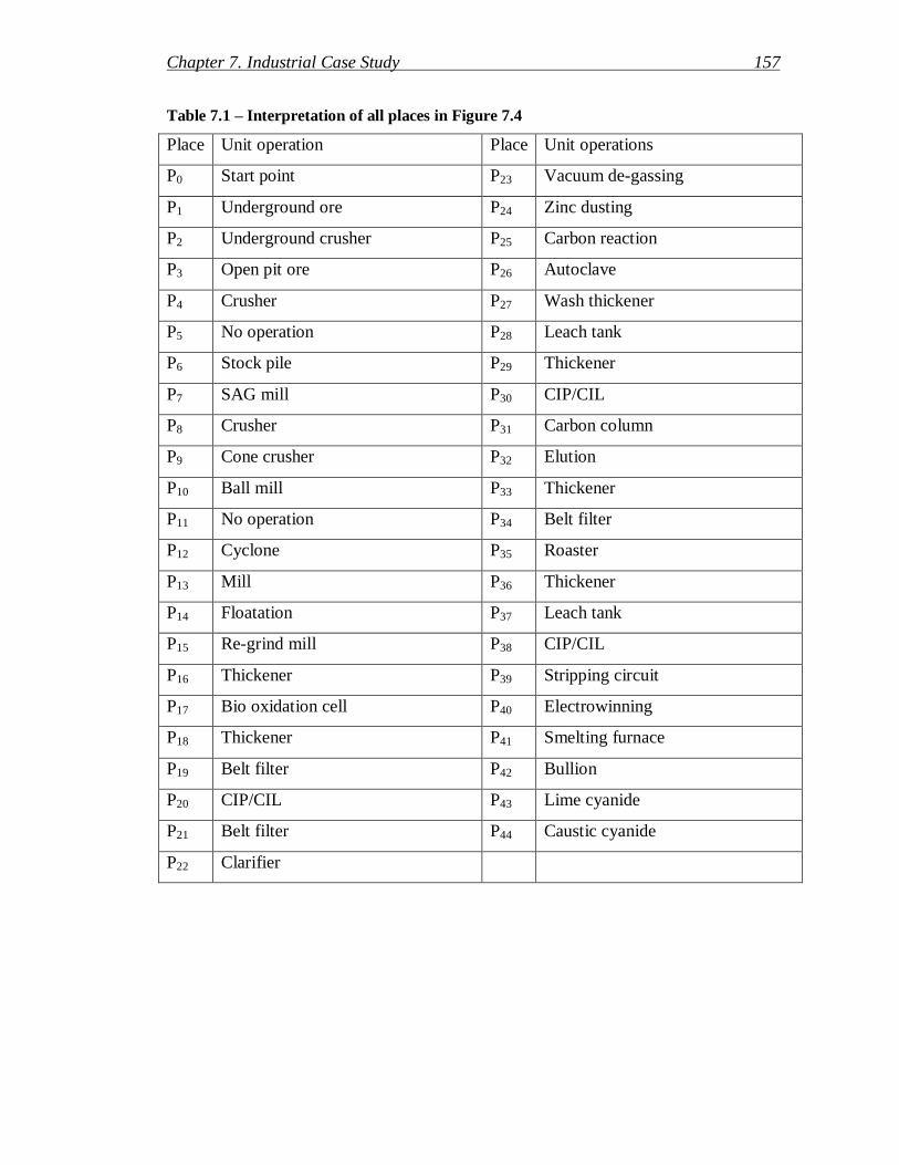
Chapter 7. Industrial Case Study 157
Table 7.1 – Interpretation of all places in Figure 7.4
Place Unit operation Place Unit operations
P0 Start point P23 Vacuum de-gassing
P1 Underground ore P24 Zinc dusting
P2 Underground crusher P25 Carbon reaction
P3 Open pit ore P26 Autoclave
P4 Crusher P27 Wash thickener
P5 No operation P28 Leach tank
P6 Stock pile P29 Thickener
P7 SAG mill P30 CIP/CIL
P8 Crusher P31 Carbon column
P9 Cone crusher P32 Elution
P10 Ball mill P33 Thickener
P11 No operation P34 Belt filter
P12 Cyclone P35 Roaster
P13 Mill P36 Thickener
P14 Floatation P37 Leach tank
P15 Re-grind mill P38 CIP/CIL
P16 Thickener P39 Stripping circuit
P17 Bio oxidation cell P40 Electrowinning
P18 Thickener P41 Smelting furnace
P19 Belt filter P42 Bullion
P20 CIP/CIL P43 Lime cyanide
P21 Belt filter P44 Caustic cyanide
P22 Clarifier

Chapter 7. Industrial Case Study 158
Table 7.2 – Interpretation of all common sub-nets and respective places
Sub-net Unit operations
1 Underground ore, underground crusher
2 Open pit ore, crusher
3 Stock pile, SAG mill, crusher
4 Cone crusher, ball mill
5 Cyclone, mill
6 Bio oxidation, thickener, belt filter, CIP/CIL, belt filter, clarifier, vacuum de-
gassing, zinc dusting
7 Carbonate reaction, autoclave, wash thickener, leach tank, thickener,
CIP/CIL, carbon columns, elution
8 Thickener, belt filter, roaster, thickener, leach tank, CIP/CIL, stripping circuit
9 Electrowinning
10 Smelting furnace, bullion
As mentioned before, to implement the new safety assessment method the proposed
place weighted stochastic Petri net is applied. In this type of Petri net each place has a
two-element weight factor holding the safety input data. The transitions are stochastic
transitions with defined not-firing probability representing the operation failure rate. The
process of calculating the input safety data and the relevant nodes in the Petri net model
are described in following section.
7.4 Safety evaluation
Two safety and risk assessment method are implemented to calculate the proposed
average safety index (Eq.6.8) for different process options in this case study.

Chapter 7. Industrial Case Study 159
7.4.1 Inherent safety assessment
In this safety evaluation method several indices have to be calculated, defined and
combined through certain equations to achieve the final I2SI for each unit operation.
The data required for these calculations are retrieved and/or generated using the
available databases, experts‟ opinions and the data applied in the similar cases in the
literature (Lees, 1996). Table 7.3 shows the safety input data and the final I2SI (Pi(w1))
computed for each unit operation. The calculation procedure has been explained briefly
in chapter 2. The detailed explanation of this method is available in Appendix A.
Next, Eq.6.6 is applied to calculate the average I2SI index for the entire production
route.
7.4.2 Probabilistic risk analysis
This method is based on two pieces of input data: failures rates and severity of the
consequences which may be obtained again using the databases, experts‟ opinions and
data in the similar cases (Lees, 1996). The risk factor related to each unit operation is
defined through Eq.2.1 . The list of the operations, respective places (Pi) and severity of
the consequences of their failures (Pi(w2)) in addition to the start transitions (Tj) and the
relevant failure rates (Tj(f)) are given in Table 7.4.

Chapter 7. Industrial Case Study 160
Table 7.3- Input data – Inherent safety assessment method
Pi ISPIi HIi Pi(w1) Pi ISPIi HIi Pi(w2)
P2 1.0 3.16 0.33 P24 1.0 4.77 0.22
P4 1.0 3.16 0.33 P25 1.0 4.77 0.22
P7 1.0 3.16 0.33 P26 1.0 3.16 0.33
P8 1.0 3.16 0.33 P27 1.0 0.73 1.41
P9 1.0 3.16 0.33 P28 5.6 2.50 2.22
P10 1.0 3.16 0.33 P29 5.6 2.92 1.91
P12 1.0 4.77 0.22 P30 5.6 2.50 2.22
P13 1.0 3.16 0.33 P31 6.0 2.44 2.46
P14 1.0 0.73 1.41 P32 6.6 3.36 1.96
P15 1.0 3.16 0.33 P33 5.6 3.00 1.85
P16 5.6 2.92 1.91 P34 2.2 2.06 1.09
P17 1.0 4.77 0.22 P35 1.0 4.77 0.22
P18 5.6 2.92 1.91 P36 5.6 2.92 1.91
P19 2.2 2.06 1.09 P37 5.6 2.50 2.22
P20 5.6 2.50 2.22 P38 5.6 2.50 2.22
P21 2.2 2.06 1.09 P39 1.0 0.73 1.41
P22 2.2 2.06 1.09 P40 6.6 3.00 2.19
P23 6.0 2.44 2.46 P41 1.0 4.77 0.22

Chapter 7. Industrial Case Study 161
Table 7.4 – Input data – probabilistic risk analysis
Pi Pi(w2) Tj Tj(f) Pi Pi(w2) Tj Tj(f)
P2 67 T1 0.015 P24 45 T23 0.020
P4 67 T4 0.015 P25 111 T25 0.020
P7 45 T7 0.015 P26 67 T26 0.015
P8 67 T8 0.015 P27 89 T27 0.005
P9 45 T9 0.015 P28 45 T28 0.015
P10 23 T10 0.015 P29 23 T29 0.010
P12 1 T12 0.020 P30 23 T29 0.010
P13 23 T13 0.015 P31 23 T30 0.010
P14 23 T13 0.015 P32 23 T31 0.015
P15 89 T14 0.005 P33 45 T33 0.015
P16 45 T15 0.010 P34 23 T34 0.010
P17 89 T16 0.020 P35 89 T35 0.020
P18 23 T17 0.015 P36 23 T33 0.015
P19 45 T18 0.010 P37 45 T36 0.010
P20 45 T19 0.010 P38 111 T37 0.010
P21 23 T20 0.010 P39 89 T38 0.005
P22 67 T21 0.010 P40 23 T39 0.015
P23 45 T22 0.010 P41 1 T40 0.020
Eq 6.7 is applied to calculate the average risk factor associated with each process
alternative.
Finally, using Eq.6.8 the Petri net model computes the average safety index related to
each production route. The penalty factor which is the number of non-responding unit
operations to the inherent safety keywords are also defined through the safety
evaluation. The developed Petri net model is executed in the Visual Studio environment
using C++ codes which are available in Appendix B. The implementation resulted in
generation of 12 possible combinations of common sub-nets and other unit operations

Chapter 7. Industrial Case Study 162
of the 3 initial processes. The average safety index and penalty factor for each option are
calculated concurrently during the route generation process. The flowsheets of these 12
processes and the respective Petri net models are given in Figure 7.5 a-l. The summary
of the results of safety analysis for these generated routes is presented in Table 7.5.
Open Pit Crusher
Cyclone
SAG Mill
Mill
Clarifier
FloatationBio Oxidation CIP/CIL
Zinc Dusting
Thickener
P-267
Re Grind
Mill
Thickener Belt Filter
Belt Filter
Vacuum
De-Gassing
Underground
Ore
Crusher
Smelting
Furnace
Stockpile
Crusher
P8
p3
p13
p12p7p6
p4
t8t12
t7
t4
p1p2
t2p0t1t0
p5t6
p11
p8
t13
p14t14 p15 p24 t24p16 p17 t17 p18t16
t15 p19 p20 p21 p22 p23t18 t19 t20 t21 t22
t23
p41 p42
t5
t41
a) Route 1

Chapter 7. Industrial Case Study 163
Open Pit Crusher
Cyclone
SAG Mill
Mill
Clarifier
FloatationBio Oxidation CIP/CIL
Zinc Dusting
Thickener
P-340
Re Grind
Mill
Thickener Belt Filter
Belt Filter
Vacuum
De-Gassing
Smelting
Furnace
Stockpile
Crusher
p3
p13
p12p7p6p4
t3 t8t12
t7t4p0 p5t6
p11
p8
t13
p14t14 p15
p24 t24p16 p17 t17 p18t16t15 p19 p20 p21 p22 p23
t18 t19 t20 t21 t22t23
p41 p42
t5
t41
b) Route 2
Open Pit Crusher
Cyclone
Ball Mill
Mill
Clarifier
FloatationBio Oxidation CIP/CIL
Zinc Dusting
Thickener
P-346
Re Grind
Mill
Thickener Belt Filter
Belt Filter
Vacuum
De-Gassing
Underground
Ore
Crusher
Smelting
Furnace
Cone
Crusher

Chapter 7. Industrial Case Study 164
p3
p13
p12p10
p4
t12
t4
p1p2
t2p0t1t0
p5 p11p9
t10t9 t11t13
p14t14 p15
p24 t24p16p17 t17 p18t16
t15 p19 p20 p21 p22 p23t18 t19 t20 t21 t22
t23
p41 p42
t5
t41
c) Route 3
Open Pit
Ore
CrusherCyclone
Ball
Mill
Mill
Clarifier
FloatationBio Oxidation CIP/CIL
Zinc
Dustig
Thickener
P-378
Re Grind
Mill
Thickener Belt
Filter
Belt Filter
Vacuum
De-Gassing
Gold Bullion Smelting Furnace
Cone
Crusher
p3
p13
p12p10p4
t12t4p0 t3 p5 p11
p9t10t9 t11
t13
p14t14 p15
p24 t24p16p17 t17 p18t16
t15 p19 p20 p21 p22 p23t18 t19 t20 t21 t22
t23
p41 p42
t5
t41
d) Route 4

Chapter 7. Industrial Case Study 165
Open Pit
Ore
Crusher
Cyclone
SAG
Mill
Mill
CIP/CIL
FloatationCarbon
Reaction
Leach
Tank
Electrowining
Thickener
P-406
Re Grind
Mill
Autoclave Thickener
Thickener
Carbon
Cooling
ElutionGold Bullion
Underground
Ore
Crusher
Smelting Furnace
Stockpile
Crusher
p3
p13
p12
p7p6
p4
t8
t12
t7
t4
p1p2
t2
p0
t1t0
p5
t6
p11
p8
p31t32
t13
p32p14t14 p15
p40
p25t26 p26
t25 p27 p28 p29
p30
p16t15 t27 t28 t29 t30 t31
p41 p42
t5
t40 t41
e) Route 5
Open Pit
Ore
Crusher
Cyclone
SAG
Mill
Mill
CIP/CIL
FloatationCarbon
Reaction
Leach
Tank
Electrowining
Thickener
P-414
Re Grind
Mill
Autoclave Thickener
Thickener
Carbon
Cooling
Elution
Gold Bullion
Smelting
Furnace
Stockpile
Crusher

Chapter 7. Industrial Case Study 166
p3
p13
p12p7p6p4
t8 t12t7t4p0 t0 p5
t6 p11
p8
p31t32
t13
p32p14t14 p15
p40
p25t26 p26
t25 p27 p28 p29
p30
p16t15 t27 t28 t29 t30 t31
p41 p42
t5
t40 t41
f) Route 6
Cyclone
Mill
CIP/CIL
FloatationCarbon
Reaction
Leach
Tank
Electrowining
Thickener
P-441
Re Grind
Mill
Autoclave Thickener
Thickener
Carbon
Cooling
Elution
Gold bullion
Smelting
Furnace
Open Pit
Ore
Crusher Ball Mill
Underground
Ore
Crusher
Cone
Crusher
p3
p13
p12p10
p4
t12
t4
p1p2
t2p0t1t0
p5 p11p9t10t9 t11
p31t32
t13
p32p14t14 p15
p40
p25t26 p26
t25 p27 p28 p29
p30
p16t15 t27 t28 t29 t30 t31
p41 p42
t5
t40 t41
g) Route 7

Chapter 7. Industrial Case Study 167
Cyclone
Mill
CIP/CIL
FloatationCarbon
Reaction
Leach
Tank
Electrowining
Thickener
P-482
Re Grind
Mill
Autoclave Thickener
Thickener
Carbon
Cooling
Elution
Gold bullion
Smelting
Furnace
Open Pit
Ore
Crusher Ball MillCone
Crusher
p3
p13
p12p10p4
t3 t12t4p0 p5 p11p9
t10t9
t11
p31t32
t13
p32p14t14 p15
p40
p25t26 p26
t25 p27 p28 p29
p30
p16t15 t27 t28 t29 t30 t31
p41 p42
t5
t40 t41
h) Route 8
Open Pit
Ore
Crusher
Crusher
CycloneSAG
Mill
Mill
Floatation
ThickenerLeach
Tank
Roaster
CIP/CIL
Stripping
Circuit
Thickener Belt Filter
Lime CyanideCaustic Cyanide
Electrowining
Smelting
Furnace
Stockpile
Gold bullionUnderground
Ore
Crusher

Chapter 7. Industrial Case Study 168
p3
p13
p12
p7p6
p4
t8
t12
t7
t4
p1p2
t2
p0
t1t0
p5
t6
p11
p8
p34
t13
t33
p33t34 p35
t36p36
p14
p37t37
t38
p38
p39 p40t39
t35
p41 p42
t5
t40 t41
p43 p44
i) Route 9
Open Pit Ore Crusher
Crusher
CycloneSAG
Mill
Mill
Floatation
Thickener
Leach Tank
Roaster
CIP/CILStripping
Circuit
Thickener Belt Filter
Lime Cyanide
Caustic Cyanide
Electrowining
Smelting
Furnace
Stockpile
Gold Bullion
p3
p13
p12p7p6p4
t3 t8 t12t7t4p0 p5
t6 p11
p8
p34
t13
t33
p33
t34p35
t36p36
p14
p37t37
t38
p38
p39 p40t39
t35
p41 p42
t5
t40 t41
p43
p44
j) Route 10

Chapter 7. Industrial Case Study 169
Cyclone
Mill
Floatation
ThickenerLeach
Tank
Roaster
CIP/CIL
Stripping
Circuit
ThickenerBelt Filter
Lime CyanideCaustic Cyanide
Electrowining
Smelting
Furnace
Gold Bullion
Open Pit
Ore
Crusher Ball
Mill
P-573
Underground
Ore
Crusher
Cone
Crusher
p3
p13
p12p10
p4
t12
t4
p1p2
t2p0t1t0
p5 p11p9t10t9 t11
p34
t13
t33
p33t34 p35
t36p36
p14
p37t37
t38
p38
p39 p40t39
t35
p41 p42
t5
t40 t41
p43 p44
k) Route 11
Cyclone
Mill
Floatation
ThickenerLeach
Tank
Roaster
CIP/CIL
Stripping
Circuit
ThickenerBelt Filter
Lime CyanideCaustic Cyanide
Electrowining
Smelting
Furnace
Gold Bullion
Open Pit
Ore
Crusher Ball
MillCone
Crusher

Chapter 7. Industrial Case Study 170
p3
p13
p12p10p4
t3 t12t4p0 p5 p11p9
t10t9 t11
p34
t13
t33
p33t34 p35
t36
p36
p14
p37t37
t38p38
p39 p40t39
t35
p41 p42
t5
t40 t41
p43 p44
l) Route 12
Figure 7.5 - Flowsheets of the 12 generated routes and respective Petri net models
Table 7.5 – Summary of the results – application of the proposed method on gold mining
case study
Route1 Route2 Route3 Route4
Average safety index 0.189 0.228 0.228 0.271
Penalty factor 11 10 10 9
Num of Equ. 19 18 18 17
Route5 Route6 Route7 Route8
Average safety index 0.256 0.294 0.336 0.382
Penalty factor 13 12 11 10
Num of Equ. 22 21 20 19
Route9 Route10 Route11 Route12
Average safety index 0.213 0.256 0.303 0.356
Penalty factor 11 10 9 8
Num of Equ. 19 18 17 16

Chapter 7. Industrial Case Study 171
7.4.3 Discussion
According to the proposed approach the process options with larger average safety index
are safer options. These production routes may be further investigated to make decision
about the optimal case. One of the other factors that may be taken into account for more
detail analysis on safer process alternatives is the penalty factor. Smaller penalty factor
shows that the larger number of unit operations in relevant process would show positive
response to the application of the inherent safety principles. The reason is that in any
process option each unit operation that does not respond to the inherent safety principles
is considered as a penalty point for that process option. Hence, the larger penalty factor
shows the larger number of not responding unit operations into inherent safety keywords
which is a negative point in regards with the safety level of a process alternative.
In Table 7.5 routes number 8 and 12 can be classified as safer possible production routes
considering the larger value of their average safety index. Among these alternatives,
route number 12 has the less number of unit operations non-responding to the inherent
safety keywords. Consequently, this process option may be consider as the optimal route
for gold production purposes.
The best option from the safety and failure risk point of view resulted by application of
the proposed method in this study is based on roasting technology. However, this route
is different from the basic option using this technology and the possibility and feasibility
of this operation needs further investigation.
7.5 Conclusion
The industrial application of the proposed integrated framework for safety evaluation
and process design was studied through the gold mining process. Three gold mines were
selected as the base cases: Kalgoorlie, Porgera, and Beaconsfield gold mines. These
three mines apply roasting technology, carbon oxidation technology and bio oxidation
technique respectively, to extract and recover gold bullion from gold ore.

Chapter 7. Industrial Case Study 172
Application of the Petri net modelling tool and creating the super-net model based on
these initial options provided the ability to automatically generate possible routes which
resulted in forming of 12 different routes for gold production. This result confirmed the
fact that there always may be a number of possible process options which are ignored by
designers during the process design phases. Creation of 9 different options in addition to
the 3 available initial cases showed the ability of proposed Petri net tool to overcome
this limitation. Furthermore, the safety and risk assessment was also implemented
concurrently with the process design and resulted in calculation of a unique final factor
representing the safety level and failure risk of each alternative. These indices may be
easily applied as decision-making factors to rank the available processes based on their
safety and failure risk and therefore choosing the optimal case among all. The developed
technique and tool in this study demonstrated enough flexibility and potential to be
applied at any stage of the process design particularly during the early phases.
Consequently, the results obtained using this approach may be used to make pro-active
decisions to improve the safety and reliability level of the processes.

Chapter 7. Industrial Case Study 173
References
Beaconsfield Gold N.L. (2007). The beaconsfield gold mine. Retrieved 15/07/2008,
2008, from http://www.beaconsfieldgold.com.au/BMJV.html
InfoMine Inc. (2008). Kargoorlie. Retrieved 22/04/2008, from
http://www.infomine.com/minesite/minesite.asp?site=kalgoorlie
Kalgoorlie Consolidated Gold Mines. (2008). Gold production, mineral processing.
Retrieved 22/04/2008, 2008, from
http://www1.superpit.com.au/pages/prod_mtc.asp
Lees, F. P. (1996). Loss prevention in the process industries: hazard identification,
assessment, and control (2nd ed.): Elsevier Butterworth-Heinemann.
Libris. (2004). Gold leaching plant. Retrieved 20/07/2008, 2008, from
www.outokumpu.com
Newmont Mining Corporation. (2008). How gold is mined. Retrieved 15/05/2008,
2008, from http://www.newmont.com/en/about/gold/howmined/index.asp
Newmont Waihi Gold. (2008). Waihi gold: The recovery process. Retrieved
15/05/2008, 2008, from
http://www.newmont.com/en/operations/australianz/waihigold/mining/recovery/i
ndex.asp
SPG Media Limited. (2008). Porgera gold mine, Papua New Guinea. Retrieved
22/04/2008, from http://www.mining-technology.com/projects/porgera/
Whitney & Whitney Inc. (2005). All about gold stocks. Retrieved 15/07/2008, from
http://www.insidemetals.com/index.php?view=mining_glossary

Chapter 8. Conclusion and Future Research 174
CChhaapptteerr 88
CCoonncclluussiioonnss aanndd FFuuttuurree RReesseeaarrcchh
8.1 Conclusions
This study has:
Reviewed and structured the available literature addressing the safety and risk
evaluation methods and tools in process industry.
Identified the major categories of safety assessment methods according to their
evaluation approaches and areas of concern. It has also investigated the major
techniques in each category in more detail.
Applied two efficient safety evaluation methods of inherent safety method and
probabilistic risk analysis as basic techniques and developed a combined
methodology which has the potential to cover a wide range of safety and
reliability issues.
Identified and described the Petri net tool as an efficient option for safety
assessment implementation to be applied in an integrated framework for safety
evaluation and process design.
Introduced the place weighted Petri net and combined it with the stochastic Petri
net and developed a competent version of Petri net tool for concurrent safety
evaluation and process design using the proposed safety and risk evaluation
technique.

Chapter 8. Conclusion and Future Research 175
Developed the integrated framework for safety evaluation and process design
with the capability to automatically generate all possible process options based
on available initial processes and implement the safety assessment
simultaneously with the process design.
The major contributions of this study are outlined in the following paragraphs.
The most significant contribution of this study was the investigation of Petri net tool as a
possible means for integration of safety evaluation into the initial phases of process
design in the process industry. It developed an automated integrated framework for
process design and safety assessment. The Petri net was introduced as an automatic
route generator for the first time in this study. It was shown that a Petri net tool is an
appropriate option for achieving integrated framework because it provides a simple
graphical modelling technique with powerful mathematical abilities for integrated
process design and concurrent safety evaluations. It has great flexibility to be adapted in
various types of processes as modelling tool and in the meantime offers the required
facilities to implement different safety and risk analysis methods. For example, it can
appropriately model continuous as well as batch processing plants. In addition, it has the
potential to implement safety assessment techniques with complicated mathematical
concepts and computations such as fuzzy approaches as well as relatively simple
methods such as probabilistic risk analysis. It also permits concurrency which means
completely independent calculations and evaluations may be executed simultaneously
through a Petri net model. Other important facilities provided by a Petri net tool
includes:
the ability to integrate all initial process options in a super-net model with
common sub-nets and individual sub-nets. These sub-nets represent the similar
unit operations and unlike unit operations existing in the different basic options,
respectively.
the possibility to be applied in various phases all over the process life-cycle with
different levels of available data.

Chapter 8. Conclusion and Future Research 176
the potential to be applied as common language amongst all contributors to
process regardless of their professional areas and levels of expertise according to
its simple and easy to understand and use approach.
This study also modified the general Petri net and introduced the place weighted Petri
net which has the ability to carry additional data related to the places. This data can be
used as the input data into other calculations such as those related to process modelling.
For example, the input safety data may be assigned to the unit operations using the
places‟ weight factors and be applied during safety evaluation which is supposed to be
done concurrently with the process modelling.
Another major contribution of this study was a new comparison factor for decision-
making purposes to evaluate safety level and failure risk in different process
alternatives, compare them together based on the provided factor and select the most
reliable option. It was shown that each of existing safety evaluation methods addresses a
limited range of safety problems such as chemical and /or physical conditions safety,
environmental safety, and reliability. Therefore, the comparison factors provided by
these methods are based on the results of evaluation of some specific aspects of safety
within the processes. If a wider range of safety issues are required to be addressed,
designers need to undertake some different safety analysis methods separately which
end up with several final safety factors. An extra effort is required to make an item-by-
item comparison or develop an appropriate method to combine these factors together
and obtain a final unique factor for decision-making purposes. This study developed a
combined measure based on two major techniques of inherent safety and probabilistic
risk analysis for each unit operation in a process. A function of all individual measures
in a process was proposed as the final index related to the entire process. This unique
index might be applied as a proper decision-making factor to rank all available
production routes based on their safety and reliability levels. This methodology provides
the opportunity to consider more safety aspects through a unique safety evaluation
process and obtain a unique final decision-making factor per process option. In addition,
the new methodology has the potential to be applied in every part of the process life-

Chapter 8. Conclusion and Future Research 177
cycle based on the available input data in each phase. Since the final factor calculated in
this method is applied for comparison purposes the extent of accuracy of the input data
does not play an important role in the whole process. However, the similarity of the data
accuracy level and resources in all processes is of great importance from the standpoint
of reliability and validity of the final factors.
As a final point, it should be mentioned that a combination of place weighted Petri net
and stochastic Petri net called place weighted stochastic Petri net was introduced in this
study for the first time and was applied to implement the proposed new safety
assessment methodology at the same time with process design. This integrated
framework provides designers with the ability to conduct process design and risk and
safety evaluation through a single process. Based on the final safety factors obtained for
each possible process option the safest and most reliable options are selected for more
feasibility studies to choose the final alternative.
8.2 Future research directions
During the period of this study, six areas of research were identified for future
investigation. These are outlined in the following part.
Testing the robustness of the results – A specific algorithm needs to be developed to
automatically run a large number of experiments to test the robustness of results.
Alternatively, a methodology can be proposed for investigating the effect of parametric
uncertainties. It requires a high load of work which was out of time and scope of this
research.
Real large-scale industrial application – Although the proposed methodology and tool
were tested on acrylic acid production and gold recovery plants, the evaluation of the
performance of this approach has been of limited scope. The acrylic acid production
pant was a small-scale plant with a limited number of unit operations adapted from the
literature for the purposes of this study. The gold recovery industrial case study was a

Chapter 8. Conclusion and Future Research 178
larger and more complicated plant which also was developed based on the available data
in the literature to serve the purpose of the current research. The input data applied in
this case was generated based on the existing data in similar cases in the literature. It is,
therefore, necessary to apply and test the proposed methodology to a number of more
complicated case studies with exact and accurate input data to strengthen the credibility
of this approach. Moreover, a real large-scale industrial case study is required to
evaluate the results of the developed approach and verify its performance from an
industrial prospective.
More mathematical investigation – The overall safety measure proposed in this study
was created based on a straightforward linear function of two existing factors. However,
there may be other more complicated functions applicable to serve the same purpose
which gives more reliable and accurate combined factors. An extensive research is
required to investigate the other possible combination techniques to develop other
mathematically valid measures with more precise performance.
Object-oriented approach – The Petri net models developed in this work were
implemented in a Visual Studio environment using the C++ coding language. Although
this approach adequately served the purposes of this study, the object oriented approach
may be considered as a better and more efficient method in this regard. In this approach
different nodes in a Petri net model can be defined as objects. A group of similar objects
form a specific class. Each object may store its own data and its own functions. The data
represents the object‟s characteristics and the functions show how an object is related
with other objects from the same or different class. The data can be used to carry safety
characteristics of the unit operations and the functions would define how different nodes
are related to each other and how safety evaluation has to be done. Therefore, to
enhance the coding part in the future studies, the use of object oriented method is
recommended.
Economic analysis – The economic efficiency of the proposed method has to be
studied. It is a very complex and demanding work that requires investigating and

Chapter 8. Conclusion and Future Research 179
developing specific economic measures to quantify the economic aspects of proposed
method and compare it with the other existing methods. According to the defined
framework and time limit of this research and the required work load to conduct
economic investigation it can be suggested as another possible area for future study
Sustainability and environmental safety consideration – The final and most
important suggestion for the future investigations is to consider sustainability and
environmental safety factors as additional concepts with great significance during the
safety evaluation process. These aspects were not included in this study as each of them
needs a separate sophisticated and extensive investigation to be adequately addressed.
According to the recent increasing concerns about environmental issues created by the
industries and the importance of sustainability considerations in industrial
developments, these concepts have to be taken into consideration during the initial
phases of the process design. While environmental considerations address the adverse
impacts of industrial activities on the surrounding environment, the sustainability
concept is about meeting the needs of the present without compromising the ability of
future generations to meet their own needs. Future investigation may, therefore, be
dedicated to developing practical methods and measures for evaluating these aspects in
industries and representing the results of this evaluation in the form of factors and
indices. These factors can be applied in conjunction with other safety and risk evaluation
factors for decision-making purposes. This will serve to perform a complete and
comprehensive evaluation of the process options integrated into process design stage. It
will demonstrate that all required evaluations related to safety, risk, reliability,
sustainability, environmental issues, and other related areas can be integrated into
process design phase using the proposed method and based on the ability of Petri nets to
execute parallel functions.

Appendix A. Indexing System 180
Appendix A
Indexing System
A.1 Integrated inherent safety index
Inherent safety concept has been introduced in literature review chapter (Chapter 2) and
applied in this research as a suitable basic method to develop a new methodology.
Moreover, Integrated Inherent Safety Index, proposed by Khan and Amyotte (2004,
2005) has been adapted as sufficient quantification technique to measure the extent of
applicability of inherent safety guidewords and their impacts on process safety. This
indexing system has been explained briefly in Chapters 2. However, for better
understanding and ease of use the calculation procedure of different indices in I2SI
system provided by Khan and Amyotte in the references (Khan & Amyotte, 2004, 2005)
is given in this appendix. All charts, graphs and tables in this appendix are adapted from
the original works.
A.1.1 Integrated inherent safety index ( I2SI ) calculation
Conceptual frameworks of I2SI and its two main components; HI and ISPI are
illustrated in Figures A.1, A.2 and A.3 respectively.

Appendix A. Indexing System 181
Figure A.1- Conceptual framework of the I2SI

Appendix A. Indexing System 182
Figure A.2- Conceptual framework of the HI
Consider one process unit and identify the
process involved and operating conditions
Identify chemicals and collect their
physiochemical characteristics
Identify type of hazards
Fire and explosion
Toxic/corrosive release& dispersion
Combination of both
Fire and
explosion hazard
Acute toxicity
hazard
Chronic
toxicity hazard
Environmental
damage
hazard
Calculate damage
radii for 50%
probability of
causing fatality
Calculate damage
radii for 50%
probability of
causing fatality
Calculate damage
radii for 50%
probability of
causing fatality
Calculate damage
radii for causing
significant
damage
Calculate
damage index Calculate
damage index
Calculate
damage index
Calculate
damage index
Combine these indices to give final damage
index (DI)
Calculate process and hazard control index
(PHCI)
Calculate hazard index (HI)
Repeat the
process for
all units

Appendix A. Indexing System 183
Figure A.3- Conceptual framework of the ISPI
Consider one process unit and identify process
involved and operating conditions
Evaluate the extent of
applicability of the guideword
Quantify the impact of
minimization ISIm
Is minimization
applicable?
Evaluate the extent of
applicability of the guideword
Quantify the impact
of substitution ISIm
Is substitution
applicable?
Evaluate the extent of
applicability of the guideword
Quantify the impact
of attenuation ISIa
Is attenuation
applicable?
Evaluate the extent of
applicability of the guideword
Quantify the impact
of simplification
ISIsi
Is simplification
applicable?
Evaluate the extent of
applicability of the guideword
Quantify the
impact of limiting
of effect ISIl
Is limiting
applicable?
ISPI = ISI / PHCI Computation of final inherent safety
index (ISI)
Repeat the process
for all units

Appendix A. Indexing System 184
The hazard index ( HI ) is comprised of two sub-indices: damage index (DI) and process
and hazard control index (PHCI). The damage index is a function of four important
parameters, namely: fire and explosion, acute toxicity, chronic toxicity, and
environmental damage. The DI is computed for each of these parameters using the
curves in Figures A.4 and A.5, which effectively convert damage radii to damage
indices by scaling up to 100.
Figure A.4- (a) Damage index graph for fire and explosion. (b) Damage index graph for
acute toxicity. (c) Damage index graph for chronic toxicity.

Appendix A. Indexing System 185
Figure A.4 were developed for the scenarios of fire and explosion, and toxic release and
dispersion for acute as well as chronic cases, for a range of chemicals using the SWeHI
approach. Within the SWeHI methodology, the damage radii term, DR, incorporates
DR1 for fire and explosion hazards and DR2 for toxic hazards. The quantification of
DR1 (fire and explosion damage radii) and DR2 (toxic damage radii) is done through a
series of steps. A brief outline of the steps is presented here.
Quantification of damage radii for fire and explosion hazards
Important steps involved in quantifying DR1 are as follows:
Classification of the various units in the plant into three main categories.
Evaluation of energy factors.
Assignment of penalties.
Estimation of damage radii (DR1), which in the SWeHI methodology is termed
as B1.
According to the first step, the various process units involved in the chemical process
industries have been classified into three different groups: (1) storage units, (2) units
involving physical operations such as heat transfer, mass transfer, phase change,
pumping and compression, and (3) units involving chemical reactions. Subsequent steps
are unique to each unit and are carried out as per the SWeHI methodology.
Quantification of damage radii for acute and chronic toxicity hazards
The parameter DR2 quantifies the toxic load (acute and/or chronic) over an area in terms
of the radius of the area (in meters) that is lethally affected by a toxic load having a 50%
probability of causing fatality. This parameter is similar to the toxic damage index B2 of
the SWeHI system and is derived using transport phenomena and empirical models
based on the quantity of chemicals involved in the unit, the physical state of the

Appendix A. Indexing System 186
chemicals, the toxicity of the chemicals, the operating conditions, and the site
characteristics.
The estimation of DR2 is done with a core factor and several penalty factors. The core
factor (G in SWeHI terminology) is dependent on the release conditions such as the state
of the chemicals involved and the plant operating conditions. Penalties are assigned
based on the chemical characteristics, operating conditions and surrounding (ambient)
characteristics. Finally, the penalties and the core factor are combined to give DR2.
Quantification of damage index for environmental damage
The DI calculation for environmental damage (Figure A.5) is adapted from the previous
work of Khan, Sadiq, and Veitch. Here, the environmental damage index is
characterized by considering the impairment impact for air, water and soil. Monographs
were developed for each environment (air, water, and soil) as shown in Figure A.5(a)–
(c). It may be seen in Figure A.5(a)–(c) that for each environment, there are three lines
classified as A, B, and C. This classification was done to account for the characteristics
of the released chemicals according to the NFPA (National Fire Protection Association)
rankings for toxic/corrosive and reactive chemicals. Chemicals having an NFPA ranking
less than 2 were classified as A, 2 and 3 as B, and 4 as C. These three DI's - one for each
environment - are combined through following equation to give the DI for
environmental damage:
DIen=Min{100,[(DIair)3+(DIwater)
3+(DIsoil)
3]
1/3}
The damage indices computed for each of these effects (fire and explosion (fe), acute
(ac) toxicity, chronic (ch) toxicity and environmental (en) impairment) are combined as
per following equation to give the final DI.
DI=Min{200,[(DIfe)2+(DIac)
2+(DIch)
2+(DIen)
2]
1/2}

Appendix A. Indexing System 187
Figure A.5- (a) Damage index graph for air pollution. (b) Damage index graph for water
pollution. (c) Damage index graph for soil pollution.
Process and hazard control index (PHCI)
The other sub-index, PHCI, is calculated for various add-on process and hazard control
measures that are required or are present in the system. The framework of the PHCI
calculation is given in Khan and Amyotte (2003). Briefly, this index is quantified
subjectively based on a mutually agreed scale among process safety experts. The index
ranges from 1 to 10 for any control arrangement and is quantified based on the necessity
of this control arrangement in maintaining safe operation. This necessity is divided into
nine groups as listed in Table A.1. For any given control system, based on necessity
(from Table A.1), an index (PHCI) may be derived from Figure A.6. This process is

Appendix A. Indexing System 188
repeated for all possible control systems. The PHCI's of these different control systems
are finally combined through following equation to give the final PHCI:
PHCI=[PHCIp+PHCIt+PHCIf+PHCIl+PHCIc+PHCIiv+PHCIb+PHCIfr+PHCIs+PHCId]
where p stands for pressure, t for temperature, f for flow, l for level, c for concentration,
iv for inert venting, b for blastwall, fr for fire resistance wall, s for sprinkler system, and
d for forced dilution.
Table A.1- Guideline to decide extent of requirement of control arrangements
Description Extent of requirement
Essential 10
Very important 9
Important 8
Not greatly important but required 7
Required 6
Requirement is moderate 5
Good if available 4
Requirement does not affect process 3
Not required 1–2

Appendix A. Indexing System 189
Figure A.6- Monograph for process and hazard control index (PHCI)
Finally, the DI is divided by the PHCI to calculate a value of hazard index (HI):
HI = DI / PHCI
Inherent safety potential index (ISPI)
Similar to the Hazard Index (HI), the inherent safety potential index (ISPI) is comprised
of two sub-indices: an inherent safety index (ISI) and a second process and hazard
control index (PHCI). To quantify the ISPI, the first step is to calculate an inherent
safety index (ISI). Again, the framework for this procedure has been previously
discussed by Khan and Amyotte (2003).
The ISI computation follows the same procedure as a HAZOP study in which
guidewords (in the present case, inherent safety principles such as minimization,
substitution, etc.) are applied to the process system. Based on the extent of applicability
and the ability to reduce the hazard, an index value is computed for each guideword.
Figure A.7 shows index values for various ranges of applicability for four of the
guidewords. To decide on the abscissa values (extent of applicability and ability to
reduce the hazard), guidelines are developed as reported in Table A.2. For the

Appendix A. Indexing System 190
guideword simplification - where the current authors experienced difficulty in
quantifying this subjective parameter - the index value can be decided using the
guidelines presented in Table A.3 (which admittedly are subjective themselves).
Figure A.7- (a) Inherent safety index for Minimization guideword. (b) Inherent safety
index for Substitution guidewod. (c) Inherent safety index for Attenuation guideword. (d)
Inherent safety index for Limiting Of guideword.

Appendix A. Indexing System 191
Table A.2- Guidelines to decide the extent of applicability of inherent safety guidewords
Description Extent Indicator
Completely applied and hazard eliminated 10
Completely applied and most significant hazard
reduced 9
Completely applied and hazard reduced 8
Completely applied and hazard moderately reduced 7
Significantly applied and hazard eliminated 6
Significantly applied and hazard reduced 5
Applicable and hazard may be eliminated 4
Applicable and hazard may be reduced 3
May be applicable and hazard may be eliminated 2
May be applicable and hazard may be reduced 1
Table A.3- Guidelines to decide ISI value for guideword simplification
Description Inherent safety index
Process simplified to large extent and hazard eliminated 100
Process simplified to large extent and most significant hazard
reduced 90
Process simplified to large extent and hazard reduced 80
Process simplified to large extent and hazard reduced moderately 70
Process simplified and hazard eliminated 60
Process simplified and hazard reduced 50
Process simplified moderately and hazard reduced 40
Process simplified moderately and hazard reduced moderately 30
No significant process simplification and hazard reduced
moderately 20
No significant process simplification and no substantial hazard
reduction 10

Appendix A. Indexing System 192
Figure A.7(a), (b) and (d) present the characterization of the ISI for minimization,
substitution and limiting of, respectively. In the case of attenuation, there are three main
operating parameters identified that control the attenuation process: (1) temperature, (2)
pressure, and (3) toxicity/corrosiveness of the chemicals. Monographs were developed
and are shown in Figure A.7(c) for these operating parameters; the index value may be
estimated based on the extent of applicability of the guideword to these operating
conditions. It is worth mentioning that the extent of attenuation guideword applicability
in the case of toxicity may be measured in terms of reduction in LC50 values
(LC50intial/LC50changed). The final inherent safety index for attenuation may be estimated
by combining the three indices through following equation:
ISIa=Min{100,[(ISItemp)3+(ISIpres)
3+(ISItoxi)
3]
1/3}
Subsequently, the ISI values calculated for the different guidewords (as defined in
Figure A.7) are combined through equation below to give a final overall ISI.
ISI=Min{200,[(ISIm)2+(ISIsu)
2+(ISIa)
2+(ISIsi)
2+(ISIl)
2]
1/2}
After analyzing the applicability of inherent safety principles (guidewords), there may
still be a requirement to install add-on process and hazard control measures. These are
accounted for using the same procedure as utilized in the hazard index (HI) calculation
procedure and discussed in an earlier section. This index is quantified subjectively based
on a mutually agreed scale among process safety experts. The index ranges from 1 to 10
for any control arrangement and is quantified based on the necessity of this control
arrangement in maintaining safe operation. This necessity is divided into nine groups as
listed in Table A.1. For any given control system, based on necessity (from Table A.1),
an index (PHCI) may be derived from Figure A.6. This process is repeated for all
possible control systems. The PHCI's of these ten different control systems are finally
combined through given to obtain the overall PHCI.

Appendix A. Indexing System 193
Finally, the inherent safety potential index (ISPI) is computed in a manner similar to the
hazard index (HI), by dividing the ISI with the PHCI:
ISPI = ISI / PHCI
A.1.2 Cost indexing procedure
In order to account for the financial aspects of inherent safety, a cost indexing system
was developed. The conceptual framework of the cost indexing procedure is shown in
the right-hand side of Figure A.1. This indexing system is comprised of two sub-indices:
a conventional safety cost index (CSCI) and an inherent safety cost index (ISCI), the
details of which are presented in the following sections.
Conventional safety cost index (CSCI)
The conventional safety cost index (CSCI) is computed as shown in this equation:
CSCI = CConvSafety / CLoss
The numerator, CConvSafety, is the sum of the costs of process control measures and add-
on (end-of-pipe) safety measures (i.e. CConvSafety=CControl+CAdd-on). Calculation of these
two components of CConvSafety is described in the sections subsequent to the following
explanation of the denominator in above equation, CLoss.
Cost of losses
For any given incident scenario, the loss index is comprised of four components:
production loss (PL), asset loss (AL), human health loss (HHL), and environmental
cleanup cost (ECC), which are governed as shown in Figure A.8. These four
components are summed to give the total cost of loss via following equation.
CLoss=CPL+CAL+CHHL+CECC

Appendix A. Indexing System 194
Figure A.8- Procedure to calculate losses
Consider one process unit and identify the
process involved and operating conditions
Identify chemicals and collect their
physiochemical characteristics
Identify type of hazards
Fire and explosion
Toxic/corrosive release& dispersion
Combination of both
Fire and
explosion hazard
Acute and Chronic
toxicity hazard
Environmental
contamination hazard
Calculate damage radius for 50% probability of causing fatality. Injury and physical damage
Estimate likely downtime in case of each hazard and select the maximum
Calculate
production
loss (CPL)
Calculate
asset loss
(CAL)
Calculate human
health loss (CHHL):
Fatality / injury
Calculate environmental clean
up cost (CECC):
Soil (CSoil)
Water (CWater)
Air (CAir)
CECC= CSoil+ CWater+ CAir
Total loss of unit (CLoss) = CPL + CAL + CHHL + CECC
Repeat the
process for
all units

Appendix A. Indexing System 195
A brief illustration of each loss type is given below.
Production loss
For a given scenario, the production loss is calculated based on production hours lost
multiplied by the cost of the each production hour:
CPL = Likely downtime (hours) × Production value ($/hour)
Asset loss
Incidents (scenarios) involving fire, explosion, or other similar events may cause loss of
physical assets, such as damage to property, loss of equipment, etc. Asset loss may be
simply calculated as:
CAL = Asset density ($/area) × Damage area
It is important to note that the damage radii employed in the current work represent a
50% probability of damage.
Human health loss
For a given scenario, human health loss is calculated in terms of the number of
fatalities/injuries and the costs associated with fatality and/or injury:
CHHL = Damage area × Population density (people/area) × Cost of fatality/injury ($)
As mentioned above, the damage radii represent a 50% probability of fatality. The
authors acknowledge that there can be high degrees of subjectiveness and discomfort
associated with assigning a dollar value to fatality and/or injury. While the value of a
human life is immeasurable, it is possible to employ indicators such as insurance costs,
rehabilitation costs, worker compensation rates, etc. Further, as the current indexing

Appendix A. Indexing System 196
procedure finds its most widespread application in relative terms, such considerations
should not introduce significant uncertainty into the results.
Environmental cleanup cost
The environmental cleanup cost for soil, water and air environments are calculated
based on the mass or volume contaminated. The mass of contaminated soil is calculated
by adopting a general soil density of 2650 kg/m3 and a depth of contamination of 0.5 m.
The volume of contaminated water is calculated by considering the contaminated area
multiplied by a 1-m depth of contamination; for contaminated air, the area multiplier is a
height of 10 m. Thus, the individual cleanup costs of:
CSoil=Mass of contaminated soil × Cleanup cost($/mass)×NH, CWater=Volume of
contaminated water×Cleanup cost ($/volume)×NH, and
CAir=Volume of contaminated air * Dilution or cleanup cost ($/volume)×NH are
summed to yield the total environmental cleanup cost via below equation.
CECC=CSoil+CWater+CAir
The term NH represents the NFPA rank of the chemical as related to health hazards. To
aid the user, we have developed a generalized table for cleanup costs (Table A.4), based
on the detailed review of remediation costs of contaminated sites conducted by Khan,
Husain and Hejazi (2004).

Appendix A. Indexing System 197
Table A.4- Range of cleanup costs for different chemical types
Pollutant Cost
Soil media (000$/ton) Water media (000$/m3) Air media (000$/m3)
Heavy metals 0.10–0.30 2.0–4.0 3.0–5.0
Metals 0.07–0.15 1.5–3.0 1.0–2.0
Organic solvents 0.05–0.08 1.0–2.0 0.5–1.5
Inorganic
solvents 0.01–0.05 0.5–1.5 0.5–1.0
Process control measure costs
The cost of process control measures may be calculated as follows:
where Ci represents the cost of a given process control measure implemented N times,
and n is the total number of control systems implemented. The cost of individual control
measures may be taken from Table A.5, which was developed through a detailed survey
of available control devices from various suppliers. To better represent the survey data,
cost is subdivided into three different categories according to the severity of operating
conditions.

Appendix A. Indexing System 198
Table A.5- Classification of process control measure costs
Control system Cost (000$)
Class A Class B Class C
Pressure control 2–4 4–9 9–15
Temperature control 1–3 3–6 6–12
Flow control 3–6 6–11 11–18
Level control 2–5 5–9 9–12
pH control 1–3 3–6 6–12
Additional control system (density control, concentration
control, etc.) 2–5 5–11 11–19
Class A: Process system/component operating in normal capacity/normal severity, and
requiring a conventional control system; for example, control measures for steam pipes,
liquid chemicals, etc.
Class B: Process system operating under high capacity/hazardous chemical/severe
operating conditions, and requiring an advanced control system; for example, control
measures for pressurized gases, flammable liquids, high gas/liquid flowrates, steam, etc.
Class C: Process system operating under very high capacity/ highly hazardous
chemical/extremely severe operating conditions, and requiring an advanced control
system; for example, control measures for liquefied gases, flammable gases, high
gas/liquid flowrates, steam, handling fine dusts, etc.
Add-on safety measure costs
In a manner similar to the process control measure costs, the cost of add-on safety
measures may be estimated as follows:

Appendix A. Indexing System 199
where Cj represents the cost of a given add-on safety measure implemented N times, and
n is the total number of add-on safety systems implemented. The cost of individual add-
on measures may be taken from Table A.6, which was developed using the same
procedure as for Table A.5.
Table A.6- Classification of add-on safety measure costs
Control system Cost (000$) of one unit
Class A Class B Class C
Alarms 0.5–1.5 2–4 4–11
Detectors 2–3.5 4–8 9–20
Firefighting equipment 6–10 10–20 21–30
Blastwall 5–9 10–16 16–25
Sprinkling system 3–5 5–15 15–25
Inert gas blanketing
system 4–10 10–17 18–30
Fire resistance wall 4–8 9–15 15–30
Other safety measures 3–7 8–14 14–32
Inherent safety cost index (ISCI)
The inherent safety cost index (ISCI) is computed through following equation:
ISCI = CInhSafety / CLoss
The denominator in above equation, CLoss, is the same as in equation for the
conventional safety cost index. The numerator, CInhSafety, is the sum of the costs of
inherent safety implementation, process control measures and add-on (end-of-pipe)
safety measures (i.e. CInhSafety=CInherent+CControl+CAdd-on). The costs of process control and

Appendix A. Indexing System 200
add-on safety measures are calculated using the formulations discussed in the preceding
sections (recognizing, of course, that these costs may change with the implementation of
inherent safety measures). A method to quantify the costs for inherent safety
implementation is described in the following section.
Inherent safety implementation costs
Inherent safety implementation costs are estimated based on the extent of application of
the inherent safety guidewords and the costs associated with their application, as shown
in Figure A.9. The cost is calculated for the application of each guideword. For example,
the cost of solvent replacement and the associated changes is estimated and thus
provides a measure of the cost of the guideword substitution. This cost is divided by a
factor called the extent of applicability, which denotes the extent to which the
guideword will eliminate/reduce the hazards. The total cost of inherent safety
implementation is represented by following equation:
CInherent=CM/EM+CS/ES+CA/EA+CSi/ESi+CL/EL
where CM, CS, CA, CSi, and CL represent the costs of minimization, substitution,
attenuation, simplification, and limitation of effects, respectively. EM, ES, EA, ESi, and
EL are the extent of applicability of the respective inherent safety principles (see Table
A.2).

Appendix A. Indexing System 201
Figure A.9- Framework for inherent safety cost computation
Consider one process unit and identify process
involved and operating conditions
Evaluate the extent of
applicability of the guideword
EM
Quantify the impact of
minimization CM
Is minimization
applicable?
Evaluate the extent of
applicability of the guideword
ES
Quantify the impact
of substitution CS
Is substitution
applicable?
Evaluate the extent of
applicability of the guideword
EA
Quantify the impact
of attenuation CA
Is attenuation
applicable?
Evaluate the extent of
applicability of the guideword
ESi
Quantify the impact
of simplification
CSi
Is simplification
applicable?
Evaluate the extent of
applicability of the guideword
EL
Quantify the
impact of limiting
of effect CL
Is limiting
applicable?
CInhSafety = CInherent + CControl +
CAdd-on
CInherent = CM / EM + CS / ES +
CA / EA + CSi / ESi + CL / EL
Repeat the process
for all units

Appendix A. Indexing System 202
A.2 Gold mining process
The I2SI related to each unit operation in gold mining case study presented in Table 7.3
in Chapter 7 has been calculated through the procedure described above. Tables A.7-
A.11 below give the detail input data applied to calculate the final I2SIs in gold mining
process.
Table A.7- Gold mining input data- I2SI and its two main sub-indices: ISPI & HI
Pi ISPI HI I2SI Pi ISPI HI I2SI
P2 1.0 3.16 0.33 P24 1.0 4.77 0.22
P4 1.0 3.16 0.33 P25 1.0 4.77 0.22
P7 1.0 3.16 0.33 P26 1.0 3.16 0.33
P8 1.0 3.16 0.33 P27 1.0 0.73 1.41
P9 1.0 3.16 0.33 P28 5.6 2.50 2.22
P10 1.0 3.16 0.33 P29 5.6 2.92 1.91
P12 1.0 4.77 0.22 P30 5.6 2.50 2.22
P13 1.0 3.16 0.33 P31 6.0 2.44 2.46
P14 1.0 0.73 1.41 P32 6.6 3.36 1.96
P15 1.0 3.16 0.33 P33 5.6 3.00 1.85
P16 5.6 2.92 1.91 P34 2.2 2.06 1.09
P17 1.0 4.77 0.22 P35 1.0 4.77 0.22
P18 5.6 2.92 1.91 P36 5.6 2.92 1.91
P19 2.2 2.06 1.09 P37 5.6 2.50 2.22
P20 5.6 2.50 2.22 P38 5.6 2.50 2.22
P21 2.2 2.06 1.09 P39 1.0 0.73 1.41
P22 2.2 2.06 1.09 P40 6.6 3.00 2.19
P23 6.0 2.44 2.46 P41 1.0 4.77 0.22

Appendix A. Indexing System 203
Table A.8- Input data for the calculation of ISI
Pi Minimization Substitution Limitation Simplification Attenuation ISI
Temp. Press. Toxi. Total
P2 1 2 1 10 1 1 0 1.26 10.4
P4 1 2 1 10 1 1 0 1.26 10.4
P7 1 2 1 10 1 1 0 1.26 10.4
P8 1 2 1 10 1 1 0 1.26 10.4
P9 1 2 1 10 1 1 0 1.26 10.4
P10 1 2 1 10 1 1 0 1.26 10.4
P12 1 2 1 10 1 1 0 1.26 10.4
P13 1 2 1 10 1 1 0 1.26 10.4
P14 1 2 1 10 1 1 0 1.26 10.4
P15 1 2 1 10 1 1 0 1.26 10.4
P16 8 20 6 50 7 8 0 9.49 55.6
P17 1 2 1 10 1 1 0 1.26 10.4
P18 8 20 6 50 7 8 0 9.49 55.6
P19 4 8 4 20 2 2 2 2.88 22.5
P20 8 20 6 50 7 8 0 9.49 55.6
P21 4 8 4 20 2 2 2 2.88 22.5
P22 4 8 4 20 2 2 2 2.88 22.5
P23 10 30 10 50 3 3 1 3.80 60.1
P24 1 2 1 10 1 1 0 1.26 10.4
P25 1 2 1 10 1 1 0 1.26 10.4
P26 1 2 1 10 1 1 0 1.26 10.4
P27 1 2 1 10 1 1 0 1.26 10.4
P28 8 20 6 50 7 8 0 9.49 55.6
P29 8 20 6 50 7 8 0 9.49 55.6
P30 8 20 6 50 7 8 0 9.49 55.6
P31 10 30 10 50 3 3 1 3.80 60.1
P32 10 40 10 50 3 3 1 3.80 65.7
P33 8 20 6 50 7 8 0 9.49 55.6
P34 4 8 4 20 2 2 2 2.88 22.5
P35 1 2 1 10 1 1 0 1.26 10.4
P36 8 20 6 50 7 8 0 9.49 55.6
P37 8 20 6 50 7 8 0 9.49 55.6
P38 8 20 6 50 7 8 0 9.49 55.6
P39 1 2 1 10 1 1 0 1.26 10.4
P40 10 40 10 50 3 3 1 3.80 65.7
P41 1 2 1 10 1 1 0 1.26 10.4

Appendix A. Indexing System 204
Table A.9- Input data for the calculation of PHCI
Pi Press. Temp. Flow level Conc. In. Ven. Blast Fire Spr. Forc. Dilu. PHCI
P2 1 1 1 1 1 1 1 1 1 1 10
P4 1 1 1 1 1 1 1 1 1 1 10
P7 1 1 1 1 1 1 1 1 1 1 10
P8 1 1 1 1 1 1 1 1 1 1 10
P9 1 1 1 1 1 1 1 1 1 1 10
P10 1 1 1 1 1 1 1 1 1 1 10
P12 1 1 1 1 1 1 1 1 1 1 10
P13 1 1 1 1 1 1 1 1 1 1 10
P14 1 1 1 1 1 1 1 1 1 1 10
P15 1 1 1 1 1 1 1 1 1 1 10
P16 1 1 1 1 1 1 1 1 1 1 10
P17 1 1 1 1 1 1 1 1 1 1 10
P18 1 1 1 1 1 1 1 1 1 1 10
P19 1 1 1 1 1 1 1 1 1 1 10
P20 1 1 1 1 1 1 1 1 1 1 10
P21 1 1 1 1 1 1 1 1 1 1 10
P22 1 1 1 1 1 1 1 1 1 1 10
P23 1 1 1 1 1 1 1 1 1 1 10
P24 1 1 1 1 1 1 1 1 1 1 10
P25 1 1 1 1 1 1 1 1 1 1 10
P26 1 1 1 1 1 1 1 1 1 1 10
P27 1 1 1 1 1 1 1 1 1 1 10
P28 1 1 1 1 1 1 1 1 1 1 10
P29 1 1 1 1 1 1 1 1 1 1 10
P30 1 1 1 1 1 1 1 1 1 1 10
P31 1 1 1 1 1 1 1 1 1 1 10
P32 1 1 1 1 1 1 1 1 1 1 10
P33 1 1 1 1 1 1 1 1 1 1 10
P34 1 1 1 1 1 1 1 1 1 1 10
P35 1 1 1 1 1 1 1 1 1 1 10
P36 1 1 1 1 1 1 1 1 1 1 10
P37 1 1 1 1 1 1 1 1 1 1 10
P38 1 1 1 1 1 1 1 1 1 1 10
P39 1 1 1 1 1 1 1 1 1 1 10
P40 1 1 1 1 1 1 1 1 1 1 10
P41 1 1 1 1 1 1 1 1 1 1 10

Appendix A. Indexing System 205
Table A.10- Input data for the calculation of DI
Pi Fire & Explosion Acute Toxicity Chronic Toxicity Environmental Damage DI
Air Water Soil Total
P2 30 10 1 0.01 0.01 0.001 0.013 31.6
P4 30 10 1 0.01 0.01 0.001 0.013 31.6
P7 30 10 1 0.01 0.01 0.001 0.013 31.6
P8 30 10 1 0.01 0.01 0.001 0.013 31.6
P9 30 10 1 0.01 0.01 0.001 0.013 31.6
P10 30 10 1 0.01 0.01 0.001 0.013 31.6
P12 40 25 7 0.01 0.1 0.001 0.100 47.7
P13 30 10 1 0.01 0.01 0.001 0.013 31.6
P14 7 2 1 0.001 0.001 0.001 0.001 7.3
P15 30 10 1 0.01 0.01 0.001 0.013 31.6
P16 25 15 1 0.01 0.01 0.001 0.013 29.2
P17 40 25 7 0.01 0.1 0.001 0.100 47.7
P18 25 15 1 0.01 0.01 0.001 0.013 29.2
P19 20 5 1 0.001 0.001 0.001 0.001 20.6
P20 20 15 1 0.001 0.001 0.001 0.001 25.0
P21 20 5 1 0.001 0.001 0.001 0.001 20.6
P22 20 5 1 0.001 0.001 0.001 0.001 20.6
P23 20 14 1 0.001 0.001 0.001 0.001 24.4
P24 40 25 7 0.01 0.1 0.001 0.100 47.7
P25 40 25 7 0.01 0.1 0.001 0.100 47.7
P26 30 10 1 0.01 0.01 0.001 0.013 31.6
P27 7 2 1 0.001 0.001 0.001 0.001 7.3
P28 20 15 1 0.001 0.001 0.001 0.001 25.0
P29 25 15 1 0.01 0.01 0.001 0.013 29.2
P30 20 15 1 0.001 0.001 0.001 0.001 25.0
P31 20 14 1 0.001 0.001 0.001 0.001 24.4
P32 30 15 1 0.01 0.01 0.001 0.013 33.6
P33 26 15 1 0.01 0.01 0.001 0.013 30.0
P34 20 5 1 0.001 0.001 0.001 0.001 20.6
P35 40 25 7 0.01 0.1 0.001 0.100 47.7
P36 25 15 1 0.01 0.01 0.001 0.013 29.2
P37 20 15 1 0.001 0.001 0.001 0.001 25.0
P38 20 15 1 0.001 0.001 0.001 0.001 25.0
P39 7 2 1 0.001 0.001 0.001 0.001 7.3
P40 26 15 1 0.01 0.01 0.001 0.013 30.0
P41 40 25 7 0.01 0.1 0.001 0.100 47.7

Appendix A. Indexing System 206
Table A.11- Input data for the calculation of PHCI after implementing inherent safety
principles
Pi Press. Temp. Flow level Conc. In. Ven. Blast Fire Spr. Forc. Dilu. PHCI
P2 1 1 1 1 1 1 1 1 1 1 10
P4 1 1 1 1 1 1 1 1 1 1 10
P7 1 1 1 1 1 1 1 1 1 1 10
P8 1 1 1 1 1 1 1 1 1 1 10
P9 1 1 1 1 1 1 1 1 1 1 10
P10 1 1 1 1 1 1 1 1 1 1 10
P12 1 1 1 1 1 1 1 1 1 1 10
P13 1 1 1 1 1 1 1 1 1 1 10
P14 1 1 1 1 1 1 1 1 1 1 10
P15 1 1 1 1 1 1 1 1 1 1 10
P16 1 1 1 1 1 1 1 1 1 1 10
P17 1 1 1 1 1 1 1 1 1 1 10
P18 1 1 1 1 1 1 1 1 1 1 10
P19 1 1 1 1 1 1 1 1 1 1 10
P20 1 1 1 1 1 1 1 1 1 1 10
P21 1 1 1 1 1 1 1 1 1 1 10
P22 1 1 1 1 1 1 1 1 1 1 10
P23 1 1 1 1 1 1 1 1 1 1 10
P24 1 1 1 1 1 1 1 1 1 1 10
P25 1 1 1 1 1 1 1 1 1 1 10
P26 1 1 1 1 1 1 1 1 1 1 10
P27 1 1 1 1 1 1 1 1 1 1 10
P28 1 1 1 1 1 1 1 1 1 1 10
P29 1 1 1 1 1 1 1 1 1 1 10
P30 1 1 1 1 1 1 1 1 1 1 10
P31 1 1 1 1 1 1 1 1 1 1 10
P32 1 1 1 1 1 1 1 1 1 1 10
P33 1 1 1 1 1 1 1 1 1 1 10
P34 1 1 1 1 1 1 1 1 1 1 10
P35 1 1 1 1 1 1 1 1 1 1 10
P36 1 1 1 1 1 1 1 1 1 1 10
P37 1 1 1 1 1 1 1 1 1 1 10
P38 1 1 1 1 1 1 1 1 1 1 10
P39 1 1 1 1 1 1 1 1 1 1 10
P40 1 1 1 1 1 1 1 1 1 1 10
P41 1 1 1 1 1 1 1 1 1 1 10

Appendix A. Indexing System 207
References
Khan, F., & Amyotte, P. (2004). Integrated inherent safety index (I2SI): A tool for
inherent safety evaluation. Process Safety Progress, 23(2), 136-148.
Khan, F., & Amyotte, P. (2005). I2SI: A comprehensive quantitative tool for inherently
safety and cost evaluation. Journal of Loss Prevention in the Process Industries,
18(4-6), 310-326.

Appendix B. C++ Codes 208
Appendix B
C++ Codes
All C++ codes which have been developed in this research to run the Petri net models
are provided in an attached CD as Appendix B.

Appendix C. Glossary Of Technical Terms 209
Appendix C
Glossary Of Technical Terms
Acidification: 1) the decrease of acid neutralizing capacity in water or base saturation in
soil caused by natural or anthropogenic processes (Cheremisinoff, 2002). 2) Ocean
acidification is the name given to the ongoing decrease in the pH of the Earth's oceans,
caused by their uptake of anthropogenic carbon dioxide from the atmosphere. Between
1751 and 1994 surface ocean pH is estimated to have decreased from approximately
8.179 to 8.104 (a change of −0.075) (Wikimedia Foundation Inc., 2001).
Additive: 1) designating or involving an equation whose terms are of the first degree
(Miller, 2009). 2) additive process: characterized or produced by addition (Miller,
2009).
Area used/species diversity: Species diversity is an index that incorporates the number
of species in an area and also their relative abundance. It is generally a much more
useful value than species richness (Wikimedia Foundation Inc., 2001).
Atomic rule: A fuzzy rule with single antecedent and consequent is called an atomic
fuzzy rule (Negnevitsky, 2002). An example of the atomic rules is as follows:
IF height is tall

Appendix C. Glossary Of Technical Terms 210
THEN weight is heavy
Battery limit: 1) battery limit refers to an area in a refinery or chemical plant
encompassing a processing unit or battery of units along with their related utilities and
services (Answers Corporation, 2009a). 2) The word "battery limit" is used to indicate
the location up to which a custodian responsibility area / piping ends. The word battery
is used to represent a set of units (Answers Corporation, 2009b). 3) “Battery limits may
be defined as a geographic boundary, real or imaginary, around the processing plant
which converts raw material to finished products” (Brennan, 1998).
Chemistry block diagram: block diagram is a diagram of a system, in which the
principal parts or functions are represented by blocks connected by lines, that show the
relationships of the blocks. They are heavily used in the engineering world in hardware
design, software design, and process flow diagrams (Wikimedia Foundation Inc., 2001).
Chemistry block diagram is the same as process flow diagram.
Compound rule: A compound fuzzy rule can have multiple antecedent and/or
consequent, for example (Negnevitsky, 2002):
IF project duration is long
AND project funding is adequate
THEN risk is high
Concurrency: In computer science, concurrency is a property of systems in which
several computations are executing simultaneously, and potentially interacting with each
other. A number of mathematical models have been developed for general concurrent
computation including Petri net, process calculi, the synchronous model and the Actor
model (Wikimedia Foundation Inc., 2001). In a Petri net model, the concurrency is
modelled by two or more transitions which are enabled and may fire independently.

Appendix C. Glossary Of Technical Terms 211
Criticality analysis: 1) a criticality analysis, which is used to chart the probability of
failure modes against the severity of their consequences. The result highlights failure
modes with relatively high probability and severity of consequences, allowing remedial
effort to be directed where it will produce the greatest value (Wikimedia Foundation
Inc., 2001). 2) Prioritizing the risks based on their probability of occurrence or the
severity of their consequences to chose the best corrective action is referred as criticality
analysis (Bowles & Pelaez, 1995).
Deductive reasoning: sometimes called deductive logic, is reasoning which constructs
or evaluates deductive arguments. In logic, an argument is said to be deductive when the
truth of the conclusion is purported to follow necessarily or be a logical consequence of
the premises and (consequently) its corresponding conditional is a necessary truth.
Deductive arguments are said to be valid or invalid, never true or false. A deductive
argument is valid if and only if the truth of the conclusion actually does follow
necessarily (or is indeed a logical consequence of) the premises and (consequently) its
corresponding conditional is a necessary truth. If a deductive argument is not valid then
it is invalid. A valid deductive argument with true premises is said to be sound; a
deductive argument which is invalid or has one or more false premises or both is said to
be not sound (unsound) (Wikimedia Foundation Inc., 2001).
Deterministic method: deterministic system or method is a system in which no
randomness is involved in the development of future states of the system. Deterministic
models thus produce the same output for a given starting condition (Wikimedia
Foundation Inc., 2001). Deterministic method ignores the probabilistic nature of the
system reliability (Mohanta et al., 2007).
Ecotoxicity (terrestrial, aquatic): Ecotoxicity, the subject of study of the field of
ecotoxicology (a portmanteau of Ecology and Toxicology) refers to the potential for

Appendix C. Glossary Of Technical Terms 212
biological, chemical or physical stressors to affect ecosystems. Such stressors might
occur in the natural environment at densities, concentrations or levels high enough to
disrupt the natural biochemistry, physiology, behaviour and interactions of the living
organisms that comprise the ecosystem.
Ecotoxicology has been defined as "the branch of toxicology concerned with the study
of toxic effects, caused by natural or synthetic pollutants, to the constituents of
ecosystems, animal (including human), vegetable and microbial, in an integral context”
(Wikimedia Foundation Inc., 2001).
Energy consumption: 1) amount of energy consumed in a process or system, or by an
organization or society (WebFinanceInc., 2009). 2) The amount of energy consumed in
the form in which it is acquired by the user. The term excludes electrical generation and
distribution losses (HIE, 2009).
Environmental cleanup cost (soil, water, air): 1) “Environmental clean-up refers to
action taken to deal with the release of a hazardous substance that could affect humans
and/or the environment. The term clean-up is sometimes used interchangeably with the
terms remedial action, response action or corrective action as opposed to the terms
preventive action or anticipatory action” (Glossary of Environment Statistics, 1997). 2)
“environmental remediation deals with the removal of pollution or contaminants from
environmental media such as soil, groundwater, sediment, or surface water for the
general protection of human health and the environment or from a brownfield site
intended for redevelopment” (Wikimedia Foundation Inc., 2001).
Eutrophication (terrestrial, aquatic): is an increase in the concentration of chemical
nutrients in an ecosystem to an extent that increases in the primary productivity of the
ecosystem. Depending on the degree of eutrophication, subsequent negative

Appendix C. Glossary Of Technical Terms 213
environmental effects such as anoxia and severe reductions in water quality, fish, and
other animal populations may occur.
Although traditionally thought of as enrichment of aquatic systems by addition of
fertilizers into lakes, bays, or other semi-enclosed waters (even slow-moving rivers),
terrestrial ecosystems are subject to similarly adverse impacts (Wikimedia Foundation
Inc., 2001).
Greenhouse effect: 1) The greenhouse effect is the heating of the surface of a planet or
moon due to the presence of an atmosphere containing gases that absorb and emit
infrared radiation. Thus, greenhouse gases trap heat within the surface-troposphere
system. This mechanism is fundamentally different from that of an actual greenhouse,
which works by isolating warm air inside the structure so that heat is not lost by
convection. The greenhouse effect was discovered by Joseph Fourier in 1824, first
reliably experimented on by John Tyndall in 1858, and first reported quantitatively by
Svante Arrhenius in 1896 (Wikimedia Foundation Inc., 2001). 2) the combustion of
fossil fuels has resulted in an increase in the carbon dioxide content of the atmosphere.
Carbon dioxide has the effect of insulating the Earth against the loss of heat, and hence
the mean temperature is in part dependent on carbon dioxide levels. The whole process
is referred to as greenhouse effect (Mobley, 2001).
Human toxicity: The degree to which a substance or mixture of substances can harm
humans or animals. Acute toxicity involves harmful effects in an organism through a
single or short-term exposure. Chronic toxicity is the ability of a substance or mixture of
substances to cause harmful effects over an extended period, usually upon repeated or
continuous exposure sometimes lasting for the entire life of the exposed organism.
Subchronic toxicity is the ability of the substance to cause effects for more than one year
(EPA, 2009).

Appendix C. Glossary Of Technical Terms 214
Nitrate toxicosis in humans occurs through enterohepatic metabolism of nitrates to
ammonia, with nitrite being an intermediate. Nitrites oxidize the iron atoms in
hemoglobin from ferrous iron (2+) to ferric iron (3+), rendering it unable to carry
oxygen. This process can lead to generalized lack of oxygen in organ tissue and a
dangerous condition called called methemoglobinemia (Wikimedia Foundation Inc.,
2001).
Inductive reasoning: is a type of reasoning which involves moving from a set of
specific facts to a general conclusion (Wikimedia Foundation Inc., 2001).
Inside battery limit (ISBL): “Inside battery limits refers to whatever happens or located
within battery limits”(Brennan, 1998).
Linguistic variable (catastrophic, critical, marginal, negligible): 1) “Loosely speaking,
a linguistic variable is a variable whose values are words or phrases”
(Andriantiatsaholiniaina et al., 2004). Catastrophic, critical, marginal and negligible can
be the examples of different linguistic variable might be used to express the severity of
the consequences of a hazardous event. The definition of each variable and its covering
area is quite subjective and may vary from one application to another.
Mass Separating Agent (MSA): mass separating agents (MSAs), such as solvents,
adsorbents, stripping agents, and ion exchange resins are used for removal of pollutants
(Garrison et al., 1995).
Multiplicative: 1) tending or having the power to multiply or increase in number or
quantity or degree (Miller, 2009). 2) of, relating to, or associated with a mathematical
operation of multiplication (Merriam-Webster, 2009).

Appendix C. Glossary Of Technical Terms 215
Noise: Noise pollution (or environmental noise) is displeasing human-, animal- or
machine-created sound that disrupts the activity or balance of human or animal life
(Wikimedia Foundation Inc., 2001).
Odour: An odor or odour (see spelling differences) is a volatilized chemical compound,
generally at a very low concentration, that humans or other animals perceive by the
sense of olfaction (Wikimedia Foundation Inc., 2001).
Outside battery limit (OSBL): “outside battery limits, also referred to as „off-site‟,
include:
Storage and handling facilities for raw materials and finished products;
Utilities generation facilities such as boilers and plant for cooling water supply,
plants for compressed air and purge gas supply, and effluent treatment facilities;
Buildings and service facilities for process plants incorporating laboratories,
workshops, offices, warehouses, cafeteria and medical facilities” (Brennan,
1998).
Ozone depletion: Ozone depletion describes two distinct, but related observations: a
slow, steady decline of about 4% per decade in the total volume of ozone in Earth's
stratosphere (ozone layer) since the late 1970s, and a much larger, but seasonal, decrease
in stratospheric ozone over Earth's polar regions during the same period. The latter
phenomenon is commonly referred to as the ozone hole (Wikimedia Foundation Inc.,
2001).
Parallelism: Parallel computing is a form of computation in which many calculations
are carried out simultaneously,[1] operating on the principle that large problems can
often be divided into smaller ones, which are then solved concurrently ("in parallel").
There are several different forms of parallel computing: bit-level, instruction level, data,
and task parallelism (Wikimedia Foundation Inc., 2001).

Appendix C. Glossary Of Technical Terms 216
Parallel tasks and functions in a system which is modelled using Petri net tool would be
executed based on the “concurrency” attribute.
Photochemical smog: Smog is a kind of air pollution; the word "smog" is a portmanteau
of smoke and fog. Classic smog results from large amounts of coal burning in an area
caused by a mixture of smoke and sulfur dioxide. Modern smog does not usually come
from coal but from vehicular and industrial emissions that are acted on in the
atmosphere by sunlight to form secondary pollutants that also combine with the primary
emissions to form photochemical smog (Wikimedia Foundation Inc., 2001).
Preventive and corrective measure: 1) preventive actions are taken to keep unit
operations working and/or extend the life of unit operations. Corrective actions are
conducted to make unit operations working again (Wikimedia Foundation Inc., 2001). 2)
Any specific operation, a modification in the design or actual replacement that prevents
a hazardous situation from occurring or corrects and repairs the consequences of a
hazardous situation may be considered as a preventive and corrective measure (Carlotti
et al., 2004).
Resource consumption: is the destruction or transformation of the resources, and hence
a change in quality and quantity, of material or energy flows (G¨oßling-Reisemann,
2008).
The National Fire Protection Association (NFPA): NFPA is a U.S. organization (albeit
with some international members) charged with creating and maintaining minimum
standards and requirements for fire prevention and suppression activities, training, and
equipment, as well as other life-safety codes and standards. This includes everything
from building codes to the personal protective equipment utilized by firefighters while
extinguishing a blaze (Wikimedia Foundation Inc., 2001).

Appendix C. Glossary Of Technical Terms 217
Universe of discourse: indicates the relevant set of entities that are being dealt with by
quantifiers. The term "universe of discourse" generally refers to the entire set of terms
used in a specific discourse (Wikimedia Foundation Inc., 2001).

Appendix C. Glossary Of Technical Terms 218
References
Andriantiatsaholiniaina, L. A., Kouikoglou, V. S., & Philips, Y. A. (2004). METHODS
Evaluating strategies for sustainable development: fuzzy logic reasoning and
sesitivity analysis. Ecological Economics, 48(2), 149-172.
Answers Corporation. (2009a). Reference Answers. Retrieved 02/10/2009, 2009, from
http://www.answers.com/topic/battery-limits
Answers Corporation. (2009b). Wiki Answers. Retrieved 01/10/2009, from
http://wiki.answers.com/Q/What_is_the_meaning_of_battery_in_battery_limits_
in_chemical_engineering
Bowles, J. B., & Pelaez, C. E. (1995). Fuzzy logic prioritization of failures in a system
failure mode, effects and criticality analysis. Process Safety Progress, 50(2),
203-213.
Brennan, D. J. (1998). Process Industry Economics: An International Perspective (Vol.
1). Warwickshire: Institution of Chemical Engineers.
Carlotti, C., Lannoy, A., Odin, S., & Procaccia, H. (2004). Detection of equipment aging
and determination of the efficiency of a corrective measure. Reliability
Engineering & System Safety, 84(1), 57-64.
Cheremisinoff, N. P. (2002). Handbook of Air Pollution Prevention and Control (Vol.
1): Elsevier Butterworth-Heinemann.
EPA. (2009). U. S. Environmental Protection Agency. Retrieved 30/09/2009, 2009,
from http://www.epa.gov/OCEPAterms/
G¨oßling-Reisemann, S. (2008). What is resource consumption and how can it be
measured? Industrial Ecology, 12(1), 10-25.
Garrison, G. W., Cooley, B. L., & El-Halwagi, M. M. (1995). Synthesis of Mass-
Exchange Networks with Multiple Target Mass-Separating Agents.
Developments in Chemical Engineering and Mineral Processing, 3(1), 31-49.
Glossary of Environment Statistics. (1997). Glossary of statistical terms. Retrieved
01/10/2009, 2009, from http://stats.oecd.org/glossary/detail.asp?ID=817
HIE. (2009). Renewable Energy in the Highlands & Islands. Retrieved 30/09/2009,
2009, from http://www.hi-energy.org.uk/index.html
Merriam-Webster. (2009). Merriam-Webster Online. Retrieved 12/11/2008, from
http://www.merriam-webster.com/
Miller, G. A. (2009). WordNet. Retrieved 12/11/2008, from
http://wordnet.princeton.edu/
Mobley, R. K. (2001). Plant Engineer's Handbook (Vol. 1): Esevier Butterworth-
Heinemann.
Mohanta, D. K., Sadhu, P. K., & Chakrabarti, R. (2007). Deterministic and stochastic
approach for safety and reliability optimization of captive power plant
aintenance scheduling using GA/SA-based hybrid techniques: A comparison of
results. Reliability Engineering & System Safety, 92(2), 187-199.

Appendix C. Glossary Of Technical Terms 219
Negnevitsky, M. (2002). Artificial intelligence: a guide to intelligent systems (first ed.
Vol. 1): Pearson Education Limited.
WebFinanceInc. (2009). BusinessDictionary.com. 2009, from
http://www.businessdictionary.com/
Wikimedia Foundation Inc. (2001). Wikipedia®: Wikimedia Foundation, Inc.