An integrated and quantitative approach to … et al 2015... · 1 An integrated and quantitative...
61
Quantifying petrophysical heterogeneity. Fitch et al. 2014 1 An integrated and quantitative approach to 1 petrophysical heterogeneity. 2 Fitch, P. J. R. 1* , Lovell, M. A. 2 , Davies, S. J. 2 , Pritchard, T. 3 and Harvey, P. K. 2 3 1 Department of Earth Science and Engineering, Imperial College London, London, United 4 Kingdom, 2 Department of Geology, University of Leicester, Leicester, United Kingdom, & 3 5 BG Group, 100 Thames Valley Park, Reading, United Kingdom. 6 * Corresponding author: Department of Earth Science and Engineering, Imperial College 7 London, London, United Kingdom (Email – [email protected], Phone – +44 (0)20 7594 8 9521) 9
Transcript of An integrated and quantitative approach to … et al 2015... · 1 An integrated and quantitative...

Quantifying petrophysical heterogeneity. Fitch et al. 2014
1
An integrated and quantitative approach to 1
petrophysical heterogeneity. 2
Fitch, P. J. R.1*, Lovell, M. A.2, Davies, S. J.2, Pritchard, T.3 and Harvey, P. K.2 3
1 Department of Earth Science and Engineering, Imperial College London, London, United 4
Kingdom, 2 Department of Geology, University of Leicester, Leicester, United Kingdom, & 3 5
BG Group, 100 Thames Valley Park, Reading, United Kingdom. 6
* Corresponding author: Department of Earth Science and Engineering, Imperial College 7 London, London, United Kingdom (Email – [email protected], Phone – +44 (0)20 7594 8 9521) 9

Quantifying petrophysical heterogeneity. Fitch et al. 2014
2
Abstract 10
Exploration in anything but the simplest of reservoirs is commonly more challenging because 11
of the intrinsic variability in rock properties and geological characteristics that occur at all 12
scales of observation and measurement. This variability, which often leads to a degree of 13
unpredictability, is commonly referred to as “heterogeneity”, but rarely is this term defined. 14
Although it is widely stated that heterogeneities are poorly understood, researchers have 15
started to investigate the quantification of various heterogeneities and the concept of 16
heterogeneity as a scale-dependent descriptor in reservoir characterization. 17
Based on a comprehensive literature review we define “heterogeneity” as the variability of an 18
individual or combination of properties within a specified space and / or time, and at a 19
specified scale. When investigating variability, the type of heterogeneity should be defined in 20
terms of grain - pore components and the presence or absence of any dominant features 21
(including sedimentological characteristics and fractures). Hierarchies of geologic 22
heterogeneity can be used alongside an understanding of measurement principles and 23
volumes of investigation to ensure we understand the variability in a dataset. 24
Basic statistics can be used to characterise variability in a dataset, in terms of the amplitude 25
and frequency of variations present. A better approach involves heterogeneity measures since 26
these can provide a single value for quantifying the variability, and provide the ability to 27
compare this variability between different datasets, tools / measurements, and reservoirs. We 28
use synthetic and subsurface datasets to investigate the application of the Lorenz Coefficient, 29

Quantifying petrophysical heterogeneity. Fitch et al. 2014
3
Dykstra-Parsons Coefficient and the coefficient of variation to petrophysical data – testing 30
assumptions and refining classifications of heterogeneity based on these measures. 31
Keywords 32
Heterogeneity, quantifying, reservoir, petrophysics, statistics 33
Acknowledgements 34
This work was initiated through a project funded by the Natural Environment Research 35
Council in collaboration with BG Group (NER/S/A/2005/13367). Thanks are due to NERC 36
for funding, and to BG Group for support, access to data and permission to publish this work; 37
in addition we acknowledge Clive Sirju, Kambeez Sobhani, and Adam Moss for helpful 38
suggestions and constructive discussions. The London Petrophysical Society is thanked for 39
access to, and permission to present the North Sea well data used in this manuscript. Mike 40
Lovell acknowledges the University of Leicester for support in the form of Academic Study 41
Leave. We are very appreciative to Stewart Fishwick, Philippe Pezard, and the late Dick 42
Woodhouse for discussions on statistical matters. Finally, we express much gratitude to the 43
three anonymous reviewers who provided detailed and constructive comments that have 44
greatly improved and widened the application of this manuscript. 45
Introduction 46
Petrophysics is the study of the (physical and chemical) rock properties and their interactions 47
with fluids (Tiab & Donaldson 2004). We can define a number of petrophysical properties, 48

Quantifying petrophysical heterogeneity. Fitch et al. 2014
4
for example porosity, saturation, and permeability, and many of these depend on the 49
distribution of other properties such as mineralogy, pore size, or sedimentary fabric, and on 50
the chemical and physical properties of both the solids and fluids. Consequently 51
petrophysical properties can be fairly constant throughout a homogeneous reservoir or they 52
can vary significantly from one location to another, in an inhomogeneous or heterogeneous 53
reservoir. This variation would be relatively easy to describe if petrophysical analysis was 54
only applied at a single scale and to a constant measurement volume within the reservoir. 55
While many petrophysical measurements are typically made in the laboratory at a core plug 56
scale (cm) or within the borehole at a log scale (m), fluid distribution is controlled at the pore 57
scale (nm to mm) by the interaction of fluids and solids through wettability, surface tension 58
and capillary forces, at the core scale by sedimentary facies, fabrics or texture (mm to m), and 59
at bed-to-seismic scales by the architecture and spatial distribution of geobodies and 60
stratigraphic elements (m to kms). Note we use the words fabric and texture here to indicate 61
generic spatial organisation or patterns. At each scale of measurement various heterogeneities 62
may exist, but it is important to note that a unit which appears homogeneous at one scale may 63
be shown to be heterogeneous at a finer-scale, and vice versa. Clearly, as more detailed 64
information is obtained, reservoir characterisation and the integration of the various data 65
types can become increasingly complex. It is important to fully understand the variability and 66
spatial distribution of petrophysical properties, so that we can understand whether there is any 67
pattern to the variability, and appreciate the significance of simple averages used in geologic 68
and simulation modelling. This is especially true in the case of complex hydrocarbon 69
reservoirs that have considerable variability. Carbonate reservoirs often fall into this 70
category, and the term heterogeneous is often used to describe a reservoir that is complex and 71

Quantifying petrophysical heterogeneity. Fitch et al. 2014
5
evades our full understanding. Indeed, an early definition states heterogeneous as meaning 72
extraordinary, anomalous, or abnormal (Oxford English Dictionary; Simpson & Weiner 73
1898). 74
Most, if not all, of the literature on reservoir characterisation and petrophysical analysis refers 75
to the heterogeneous nature of the reservoir under investigation. Heterogeneity appears to be 76
a term that is readily used to suggest the complex nature of the reservoir, and authors often 77
assume the reader has a pre-existing knowledge and understanding of such variability. No 78
single definition has been produced and consistently applied. Researchers have started to 79
investigate the quantification of various heterogeneities and the concept of heterogeneity as a 80
scale-dependent descriptor in reservoir characterization (Frykman 2001; Jennings & Lucia 81
2003; Pranter et al. 2005; Westphal et al. 2004). 82
Here we review what heterogeneity means, and how it can be described in terms of 83
geological attributes before discussing how the scale of geological heterogeneity can be 84
related to the measurement volumes and resolution of traditional subsurface data types. We 85
then discuss using a variety of statistical techniques for characterising and quantifying 86
heterogeneity, focussing on petrophysical heterogeneities. We focus here on the principles 87
and controls on the statistics and measures, before applying these to real reservoir data in four 88
case studies. In doing so, we consider approaches used in a range of scientific disciplines 89
(primarily the environmental sciences and ecology) to explore definitions and methods which 90
may be applicable to petrophysical analysis. These statistical techniques are then applied to 91
reservoir sub-units to investigate their effectiveness for quantifying heterogeneity in reservoir 92
datasets. 93

Quantifying petrophysical heterogeneity. Fitch et al. 2014
6
Defining Heterogeneity 94
Heterogeneity refers to the quality or condition of being heterogeneous, and was first defined 95
in 1898 as difference or diversity in kind from other things, or consisting of parts or things 96
that are very different from each other (Oxford English Dictionary; Simpson & Weiner 97
1989). A more modern definition is something that is diverse in character or content (Oxford 98
Dictionaries, 2014). This broad definition is quite simple and does not comment on the spatial 99
and temporal components of variation, nor does it include a consideration of directional 100
dependence, often referred to as isotropy and anisotropy. Other words or terms that may be 101
used with, or instead of, heterogeneity include; complexity, deviation from a norm, 102
difference, discontinuity, randomness, and variability. 103
Nurmi et al. (1990) suggest that the distinction between homogeneous and heterogeneous is 104
often relative, and is based on economic considerations. This highlights how heterogeneity is 105
a somewhat variable concept which can be changed or re-defined to describe situations that 106
arise during production from a reservoir, and is heavily biased by the analyst’s experience 107
and expectations. Li and Reynolds (1995) and Zhengquan et al. (1997) state that 108
heterogeneity is defined as the complexity and/or variability of the system property of interest 109
in three-dimensional space, while Frazer et al. (2005) define heterogeneity, within an 110
ecological model, as variability in the density of discrete objects or entities in space. These 111
definitions suggest that heterogeneity does not necessarily refer to the overall system, or 112
individual rock/reservoir unit, but instead may be dealt with separately for individual units, 113
properties, parameters and measurement types. 114
Quantifying petrophysical heterogeneity. Fitch et al. 2014
7
Frazer et al. (2005) commented that heterogeneity is an inherent, ubiquitous and critical 115
property that is strongly dependent on scales of observation and the methods of measurement 116
used. They studied forest canopy structure and stated that heterogeneity is the degree of 117
departure from complete spatial randomness towards regularity and uniformity. This may 118
seem, at first, counterintuitive because heterogeneity is commonly regarded as being 119
complete spatial randomness. Here, the introduction of regular features, such as bedding in a 120
geological context, adds to the heterogeneous nature of the formation in a structured or 121
anisotropic manner. Nurmi et al. (1990) suggest that heterogeneity, in electrical borehole 122
images, refers to elements that are distributed in a non-uniform manner or composed of 123
dissimilar elements/constituents within a specific volume. Therefore, as well as looking at a 124
specific element or property, it is also suggested that the volume of investigation influences 125
heterogeneity, alluding to the scale-dependence of heterogeneities. Interestingly, Dutilleul 126
(1993) comments that a shift of scale may create homogeneity out of heterogeneity, and vice-127
versa, and suggests that heterogeneity is the variation in density of measured points compared 128
to the variation expected from randomly spread points. In a discussion of the relationship 129
between scale and heterogeneity in pore size, Dullien (1979) suggests that to be a truly 130
homogeneous system random subsamples of a population should have the same local mean 131
values. Lake and Jensen (1991) provide a flow-based definition in their review of 132
permeability heterogeneity modelling within the oil industry. In this latter case, heterogeneity 133
is defined as the property of the medium that causes the flood front to distort and spread as 134
displacement proceeds; in this context the medium refers to the rock, and fluid front is the 135
boundary between displacing and displaced fluids. Thus many authors provide the foundation 136
in which we begin to see that heterogeneity may be a quantifiable term. 137

Quantifying petrophysical heterogeneity. Fitch et al. 2014
8
Pure homogeneity, with regard to a reservoir rock, can be visualised in a formation that 138
consists of (1) a single mineralogy with (2) all grains of similar shapes and sizes with (3) no 139
spatial organization or patterns present; in this example, similar grain shapes and sizes, 140
together with lack of spatial patterns would lead to a uniform distribution of porosity and 141
permeability. Therefore, ignoring the scalar component of heterogeneity for a moment, there 142
are two contrasting examples of heterogeneity in a reservoir rock (Figure 1). The first 143
example is a formation of consistent mineralogy and grain characteristics that has various 144
spatial patterns (for example bedding, foresets, syn-sedimentary faulting, or simply grain 145
packing). The second example has no spatial organisation (it is massive) but has variable 146
mineralogy and grain size and shape, i.e. it is a poorly sorted material. Both are clearly not 147
homogeneous but which has the stronger heterogeneity? Quantifying the degree of 148
heterogeneity would enable these two different systems to be differentiated from each other, 149
and in turn these values may be related to other characteristics such as reservoir quality. In 150
attempting to quantify heterogeneity we can consider several approaches. It is probably best, 151
however, to start by defining the degree of heterogeneity in relation to the nature of the 152
investigation; for example in a study of fluid flow, sedimentological structures may be of 153
more importance than variation in mineralogy. In contrast in an investigation of downhole 154
gamma ray variability the mineralogical variability (or strictly chemical variability of 155
potassium, thorium and uranium) would be more relevant than any spatial variation. 156
Lake and Jensen (1991) suggest that there are five basic types of heterogeneity in earth 157
sciences; (1) Spatial - lateral, vertical and three-dimensional, (2) Temporal - one point at 158
different times, (3) Functional - taking correlations and flow-paths into account, (4) Structural 159

Quantifying petrophysical heterogeneity. Fitch et al. 2014
9
- either unconformities or tectonic elements, such as faults and fractures, and (5) 160
Stratigraphic. Formations may have regular and penetrative features such as bedding and 161
cross-bedding, or alternatively less regularly distributed features, including ripples, 162
hummocky cross-bedding, and bioturbation. The intensity, frequency and orientation of such 163
features may additionally reflect repetition or repetitive patterns through the succession. A 164
heterogeneity, in terms of the grain component, may appear rhythmic or repeated, patchy, 165
gradational / transitional, or again it may be controlled by depositional structures (Nurmi et 166
al. 1990). 167
Homogeneity and heterogeneity can be considered as end members of a continuous spectrum, 168
defining the minimum and maximum heterogeneity, with zero heterogeneity equating to 169
homogeneity. There are a number of characteristics that occur in both end-member examples 170
provided above (for example vertical rhythmicity in terms of bedding or grain size 171
distribution). Neither end-member is obviously more heterogeneous than the other; there may 172
indeed be a relative scale difference between the two examples. Some researchers may 173
perceive a regularly structured system, for example a laminated or bedded reservoir, as 174
homogeneous because these structures are spatially continuous and occur throughout the 175
formation. The presence of structures within a formation is, however, more commonly 176
interpreted as a type of heterogeneity, regardless of how regular their distribution. In this 177
scenario, the structures represent deviation from the homogeneous mono-mineralic ‘norm’. 178
Equally the concept of increased heterogeneity could be viewed as an increase in the random 179
mixing of components of a formation. Here, as the formation becomes more heterogeneous 180
there is less spatial organization present, so that the formation has the same properties in all 181

Quantifying petrophysical heterogeneity. Fitch et al. 2014
10
directions, i.e., it is isotropic. Although the rock is more heterogeneous, the actual reservoir 182
properties (such as the porosity distribution) become more homogeneous throughout the 183
reservoir as a whole. 184
If grain-size alone varies, two possible extremes of heterogeneity may occur. An example 185
where there is a complete mix of grain sizes that show no evidence of sorting would be 186
classified as a heterogeneous mixture in terms of its components. The mixture itself would 187
appear isotropic, however, because on a larger-scale the rock properties would be the same in 188
all directions (in the sense of a transverse isotropic medium). If this mixture of grain sizes 189
was completely unsorted then the grains would be completely randomly distributed and the 190
rock would appear homogeneous at a larger scale. In another example where a formation has 191
continuous and discontinuous layers of different grain sizes, the individual layers of similar 192
grain size may appear homogeneous, however if looking at a contact between two layers, or 193
the complete formation, then the heterogeneity will be much more obvious. This may be 194
classed as a ‘structural’ or ‘spatial’ heterogeneity, again depending upon the scale of 195
investigation. 196
When defining a measure of how heterogeneous a system property is, it is important to 197
consider only those components of heterogeneity that have a significant impact on reservoir 198
properties and production behaviour / reservoir performance. This leads to the discussion of 199
heterogeneity as a scale-dependent descriptor in the next section. 200
Scale and measurement resolution 201

Quantifying petrophysical heterogeneity. Fitch et al. 2014
11
Regardless of reservoir type, geological heterogeneity exists across a gradational continuum 202
of scales (Nichols 1999; Moore 2001). Observations from outcrop analogues have been used 203
to characterise and quantify these features (examples for carbonate outcrops include Mutti et 204
al. 1996; Pomar et al. 2002; Badenas et al. 2010; Cozzi et al. 2010; Koehrer et al. 2010; 205
Palermo et al, 2010; Pierre et al. 2010; Amour et al. 2012). Hierarchies of heterogeneity are 206
now frequently used to classify these heterogeneities over levels of decreasing magnitude 207
within a broad stratigraphic framework. Heterogeneity hierarchies have been developed for 208
wave-influenced shallow marine reservoirs (e.g. Kjønsvik et al. 1994; Sech et al. 2009), 209
fluvial reservoirs (e.g. Jones et al. 1995), fluvio-deltaic reservoirs (e.g. Choi et al. 2011), and 210
carbonate reservoirs (e.g. Jung & Aigner 2012). These hierarchies break the continuum of 211
scales of geologic and petrophysical properties into key classes or ranges. 212
A single property can differ across all scales of observation. Porosity in carbonates is an 213
example of a geological property that can exist, and vary, over multiple length-scales. In 214
carbonate rocks pore size can be seen to vary from less than micrometre-size micro-porosity 215
(e.g., North Sea chalks; Brasher & Vagle 1996) to millimetre-scale inter-particle and 216
crystalline porosity (e.g., carbonate reservoirs of the Middle East, Lucia 1995, Ramamoorthy 217
et al. 2008; offshore India, Akbar et al. 1995; and the microbialite build-ups of offshore 218
Brazil, Rezende et al. 2013) . Vugs are commonly documented to vary in size from 219
millimetre to tens of centimetres (e.g., Nurmi et al. 1990). Additional dissolution and erosion 220
may create huge caves, or “mega-pores” (often being metres to kilometres in size, e.g., Akbar 221
et al. 1995; Kennedy 2002). 222

Quantifying petrophysical heterogeneity. Fitch et al. 2014
12
In order to investigate heterogeneity at different scales and resolutions, the concept of “scale” 223
and how it relates to different parameters is considered. Figure 2 illustrates the scales of 224
common measurement volumes and their relationship to geological features observed in the 225
subsurface. While geological attributes exist across the full range of length-scale (mm – km 226
scale; e.g. van Wagoner et al. 1990; Jones et al. 1995; Kjønsvik et al. 1994; Frykman and 227
Deutsch 2002; Sech et al. 2009; Choi et al. 2011; and Jung & Aigner 2012), subsurface 228
measurements typically occur at specific length-scales depending upon the physics of the tool 229
used. For example, seismic data at the kilometre scale, well logs at the centimetre to metre 230
scale, and petrophysical core measurements at millimetre to centimetre scales. In general the 231
insitu borehole and core measurement techniques are considered to interrogate a range of 232
overlapping volumes, but in reality a great deal of “white space” exists between individual 233
measurement volumes (Figure 2). How a measurement relates to the scale of the underlying 234
geological heterogeneity will be a function (and limitation) of the resolution of the 235
measurement device or tool used. The analyst or interpreter should ensure that appropriate 236
assumptions are outlined and documented. 237
The issue of how the scale and resolution of a measurement will be impacted by 238
heterogeneity can be represented through the concept of a Representative Elementary 239
Volume (REV) to characterise the point when increasing the size of a data population no 240
longer impacts the average, or upscaled, value obtained (Bear 1972, Bachmat & Bear 1987). 241
The REV concept lends itself to an extensive discussion on upscaling and the impact of 242
heterogeneity on flow behaviour, which are beyond the current scope of this study. Examples 243

Quantifying petrophysical heterogeneity. Fitch et al. 2014
13
of previous studies into REV, sampling and permeability heterogeneity include Haldorsen 244
(1986), Corbett et al. (1999), Nordahl & Ringrose (2008), Vik et al. (2013). 245
Different wireline log measurements, for example, will respond to, and may capture, the 246
different parts or scales of geological heterogeneity (Figure 2C and 3). The geological 247
features that exist below the resolution of tools shown in Figure 2 will in effect be averaged 248
out in the data (Ellis & Singer 2007). Figure 3 shows how the heterogeneity of a formation 249
can vary depending on the scale at which we sample the formation. Examples are shown for 250
three distinct geological features; beds of varying thickness only (Figure 3A), a set of graded 251
beds, again, of varying thicknesses (Figure 3B), and a “large” and “small” core sample for 252
two sandstone types (Figure 3C). A quantitative assessment of whether a formation appears 253
homogeneous or heterogeneous to the measurement tool as it travels up the borehole is 254
possible. The degree of measured heterogeneity will also change as the measurement volume 255
changes (e.g. Figure 3A and B); shallow measurements (e.g. bulk density or micro resistivity) 256
will sample smaller volumes, whereas deep measurements (e.g. gamma radiation, acoustic 257
travel time or deep resistivity) will sample large volumes. 258
Assessment of thinly bedded siliciclastic reservoirs highlights the issues of correlating 259
geological-petrophysical attributes to petrophysical measurement volumes. Thin beds are 260
defined geologically as being less than 10 cm thick (Campbell 1967), whereas a “modern” 261
petrophysical thin bed is referred to as less than 0.6 m in thickness, and is defined to reflect 262
the vertical resolution of most porosity and resistivity logs (Qian & Zhong 1999; Passey et al. 263
2006). The micro-resistivity logs (including dipmeter and borehole electrical imaging logs) 264
have a higher vertical resolutions and so can recognise thin beds on a scale that is more 265

Quantifying petrophysical heterogeneity. Fitch et al. 2014
14
consistent with the geological scale (Cheung et al. 2001; Passey et al. 2006). Figure 3 (A and 266
B) illustrates how alternating high and low porosity thin beds, that are significantly below the 267
resolution of typical wireline well logs, would appear as low variability within the 268
measurement volume. 269
Up-scaling from core measurements to petrophysical well log calibration, and eventually to 270
subsurface and flow simulation models of the reservoir at circa seismic-scale is a related 271
topic. This process of upscaling represents a change of scale and hence properties may 272
change from being heterogeneous at one scale to homogeneous at another scale. A discussion 273
of up-scaling is beyond the scope of this paper. 274
To summarise, ‘heterogeneity’ may be defined as the complexity or variability of a specific 275
system property in a particular volume of space and/or time. Effectively there is the intrinsic 276
heterogeneity of the property itself (e.g. porosity or mineralogy) and the measured 277
heterogeneity as described by the scale, volume and resolution of the measurement technique. 278
Evaluating Heterogeneity 279
Having defined heterogeneity, we consider a variety of statistical techniques that can be used 280
to quantify heterogeneity. Techniques are grouped into two themes: (1) characterising the 281
variability in a dataset and; (2) quantifying heterogeneity through heterogeneity measures. 282
Firstly we illustrate how standard statistics can be used to characterize the variability or 283
heterogeneity in a carbonate reservoir. Secondly we use four simple synthetic datasets to 284
illustrate the principles of and controls on three common heterogeneity measures, before 285
Quantifying petrophysical heterogeneity. Fitch et al. 2014
15
applying the heterogeneity measures to (a) the porosity data from two carbonate reservoirs, 286
(b) a comparison of core and well log-derived porosity data in a clastic reservoir, (c) core 287
measured grain density as a proxy for mineralogic variation in a carbonate reservoir, and (d) 288
gamma ray log-derived bedding heterogeneities in a clastic reservoir.. 289
Characterising the variability of the dataset 290
The core-calibrated well log-derived porosity data from an Eocene-Oligocene carbonate 291
reservoir are used to illustrate the concepts for characterising heterogeneity (Figure 4). 292
Formation A is c.75 m in vertical thickness, and is dominated by wackestone and packstone 293
facies, with carbonate mudstone & grainstone interbeds. Formation B is c.54 m in vertical 294
thickness, and is composed of grain-rich carbonate facies (predominantly comprising 295
packstone to grainstone facies). Micro- and matrix-porosity dominate Formations A and B in 296
the form of vugs, inter- and intra-granular porosity (Reddy et al. 2004; Wandrey 2004; Naik 297
et al. 2006; Barnett et al. 2010). Metre-thick massive mudstone interbeds are observed toward 298
the top of Formation A. The mudstone is suggested to be slightly calcareous and dolomitic in 299
nature, with trace disseminated pyrite (Thakre et al. 1997; Estebaan 1998). 300
A simple glance at the wireline data for this reservoir (e.g., Figure 4) suggests Formation-A is 301
more variable or “heterogeneous”. An early step in completing a routine petrophysical 302
analysis is often to produce cross plots of the well log data; these give additional visual clues 303
as to the presence of heterogeneities within the data (e.g. Figure 5). Formation-A has a 304
diverse distribution of values across the bulk density – neutron porosity cross plot, indicating 305
its more heterogeneous character when compared to Formation-B, which is more tightly 306

Quantifying petrophysical heterogeneity. Fitch et al. 2014
16
clustered (Figure 5). The bulk density – neutron porosity cross plot reflects the varied facies 307
and porosity systems of Formation-A, in comparison to the carbonate packstone-grainstone 308
dominated Formation-B with a more uniform porosity system. 309
Basic statistics can be used to characterise the variation in distribution of values within a 310
population of data. The basic statistics (Table 1) and histogram (Figure 6) for the values of 311
wireline log derived porosity for Formations A and B clearly reflect different variability 312
within the data populations. Log-derived porosity in Formation A is skewed toward lower 313
values around a mean value of 8.5 %, with a moderate kurtosis (Figure 6, Table 1). The 314
statistics for the log-derived porosity of Formation B records a tendency toward higher values 315
(negatively skewed) around a mean of 21.9 % and a stronger kurtosis (Figure 6, Table 1). The 316
standard deviation, of values around the mean, is moderate for both Formations. This 317
suggests that values are neither tightly clustered nor widely spread around the mean, although 318
we note that the standard deviation for Formation B is one unit lower. 319
These basic statistics can be used to characterise variation within a dataset, producing a suite 320
of numerical values that describe data distributions. However, we need to complete and 321
understand the full suite of statistical tests to achieve what is still a fairly general numerical 322
characterisation of heterogeneity. We note that we could not use a similar suite of statistics to 323
directly compare the variability between different data types that occur at different scales as 324
the range of values has strong control on the outputs, for example comparing the variability in 325
porosity (on a theoretical maximum scale of 0 to 100) with permeability (which for a 326
conventional reservoir can vary between over several orders of magnitude, from close to 0 to 327
1000s mD). Thus, when using basic statistics, there is no single value to adequately define the 328

Quantifying petrophysical heterogeneity. Fitch et al. 2014
17
quantitative heterogeneity of a dataset as being “x”, that would enable direct comparison of 329
different well data, formations and reservoirs. Instead, to achieve a direct heterogeneity 330
comparison that is both robust and useful we must consider established heterogeneity 331
measures. 332
Quantifying Heterogeneity: heterogeneity measures 333
Measures used in quantifying heterogeneity use geostatistical techniques to provide a single 334
value to describe the heterogeneity in a dataset. Published heterogeneity measures, such as 335
the coefficient of variation and the Lorenz Coefficient, have been in common use throughout 336
most scientific disciplines, and are frequently used in establishing porosity and permeability 337
models in exploration (e.g. Dykstra & Parsons 1950; Lake & Jensen 1991; Reese 1996; 338
Jensen et al. 2000; Elkateb et al. 2003; Maschio & Schiozer 2003; Sadras & Bongiovanni 339
2004; Sahni et al. 2005). 340
Four simple synthetic datasets (Table 2) are used to illustrate the impact of common types of 341
variability in a dataset on the heterogeneity measures. These measures are then applied to 342
specific heterogeneities in a series of case studies. Of the synthetic datasets, Dataset (i) is 343
homogeneous with no internal variation, Dataset (ii) is composed of two values representing 344
a high and low setting, Dataset (iii) comprises a simple linear increase in values, and Dataset 345
(iv) represents an exponential increase in values (Table 2). 346
Coefficient of Variation 347
The coefficient of variation (Cv) is a measure of variability relative to the mean value. The 348
most commonly used method for calculating the coefficient of variation is shown below 349

Quantifying petrophysical heterogeneity. Fitch et al. 2014
18
(Equation 1), although numerous variations on this approach can be found in published 350
literature. A homogeneous formation will have a coefficient of variation of zero, with the 351
value increasing with heterogeneity in the dataset (Elkateb et al. 2003). 352
𝐶𝐶 = √𝜎2
�̅� (Equation 1) 353
[Where: Cv is the coefficient of variation, √𝜎2 is the standard deviation, and �̅� is the mean] 354
For our synthetic test datasets, we see coefficient of variation increase with heterogeneity; (i) 355
Cv = 0, (ii), Cv = 0.35, (iii) Cv = 0.55, and (iv) Cv = 2.82. 356
The Lorenz Coefficient 357
The original Lorenz technique was developed as a measure of the degree of inequality in the 358
distribution of wealth across a population (Lorenz 1905). Schmalz and Rahme (1950) 359
modified the Lorenz Curve for use in petroleum engineering by generating a plot of 360
cumulative flow capacity against cumulative thickness, as functions of core measured 361
porosity and permeability. Fitch et al. (2013) investigated the application of the Lorenz 362
technique directly to porosity and permeability data. In our application of the Lorenz 363
Coefficient, and to allow comparison of the heterogeneity in a single data type between the 364
different measures, the cumulative of the property of interest (e.g., porosity), sorted from high 365
to low values, is plotted against cumulative measured depth increment (Figure 7A; Fitch et al. 366
2013, and Figure 7B, the synthetic dataset considered here). In a purely homogeneous 367
formation, the cumulative property will increase by a constant value with depth, this is known 368
as the “line of perfect equality” (Sadras & Bongiovanni 2004). An increase in the 369

Quantifying petrophysical heterogeneity. Fitch et al. 2014
19
heterogeneity of the property will cause a departure of the Lorenz Curve away from the line 370
of perfect equality. The Lorenz Coefficient (Lc) is calculated as twice the area between the 371
Lorenz Curve and the line of perfect equality; a pure homogeneous system will return a 372
Lorenz Coefficient of zero, while maximum heterogeneity is shown by a Lorenz Coefficient 373
value of one (Figure 7A). 374
The Lorenz Coefficients generated for our synthetic test datasets demonstrate some of the key 375
features of the Lorenz technique; Dataset (i) matches the line of perfect equality (Figure 7B), 376
returning an Lorenz Coefficient of zero, Datasets (ii) and (iii) return Lorenz Coefficient 377
values of 0.16 and 0.25, respectively, and the exponential data of set (iv) returns a Lorenz 378
Coefficient value of 0.86, and is clearly visible as the most heterogeneous data with the 379
largest departure from the line of perfect equality (set (i)) on Figure 7B. 380
Dykstra-Parsons Coefficient 381
The Dykstra-Parsons Coefficient (VDP) is commonly used in the quantification of 382
permeability variation. A method for calculating VDP, provided by Jensen et al. (2000), 383
begins by ranking the property of interest (e.g., porosity) in order of decreasing magnitude. 384
We have followed the method presented by Maschio and Schiozer (2003) to assign 385
probability values; for each individual value calculate the percentage of values greater than, 386
or the ‘cumulative probability’, so that the probability of X is P(x≤X). The original 387
permeability values are then plotted on a log probability graph with the cumulative 388
probability values (Figure 8A). The slope and intercept of a line of best fit, for all data, from 389
this plot is then used to calculate the 50th and 84th probability percentile, which are used in 390
Equation 3 to derive VDP. Here, we assume a log-normal distribution, so that the 391

Quantifying petrophysical heterogeneity. Fitch et al. 2014
20
Log(property) value at the 84th percentile represents one standard deviation away from the 50 392
% probability (Machio & Schiozer 2003). As heterogeneity increases the slope of the line of 393
best fit increases along with the difference between the 50th and 84th percentile, and 394
subsequently the value of VDP (Figure 8A). 395
𝑉𝐷𝐷 = 𝑥50−𝑥84𝑥50
(Equation 3) 396
[Where x50 is the 50th property percentile, and x84 is the 84th property percentile] 397
Our synthetic datasets show significant differences in the Dykstra-Parsons plots produced 398
(Figure 8B) and resultant Dykstra-Parsons values; set (i) VDP = 0.0, set (ii) VDP = 0.31, set 399
(iii) VDP = 0.57, and set (iv) VDP = 0.99. 400
Selection of Appropriate Heterogeneity Measures 401
The key advantage to using a heterogeneity measure is the ability to define the heterogeneity 402
of a dataset as a single value, allowing direct comparison between different data types, 403
reservoir units (formations) and fields. 404
The coefficient of variation provides the simplest technique for generating a single value 405
measure of heterogeneity, with no data pre-processing required. By calculating the standard 406
deviation as a fraction of the mean value we are looking at the variability within the data 407
distribution, removing the influence of the original scale of measurement. As such the 408
coefficient of variation should provide a more appropriate measure of the heterogeneity of a 409
dataset than the basic statistics (as in Table 1), that can be compared between different 410

Quantifying petrophysical heterogeneity. Fitch et al. 2014
21
measurement types and scales of observation. Lake and Jensen (1991) comment that the 411
estimate of Cv is negatively biased, suggesting that the Cv estimated from data will be 412
smaller than the value for the true population. Sokal and Rohlf (2012) suggest that care 413
should be used in applying the coefficient of variation to ‘small samples’ and provide a 414
simple correction. In addition the coefficient of variation should only be applied to data 415
which exist on a ratio scale with a fixed zero value, for example it is not appropriate for 416
temperature measurement in Fahrenheit or Celsius (Sokal & Rohlf 2012). The coefficient of 417
variation (Cv) increases with heterogeneity to infinity as no upper limit is defined in the 418
calculation (Figure 9). Lake and Jensen (1991) suggest that this is a major advantage in use of 419
the coefficient of variation as a heterogeneity measure, in that it can distinguish extreme 420
variation. However, we favour a heterogeneity measure with defined upper and lower limits, 421
allowing a clear comparison of variation in different datasets with different scales, resolutions 422
and hypothetical end-member values across a similarly scaled range. We note that Jensen and 423
Lake (1988) suggest that high levels of heterogeneity are compressed in the case of the 424
Dykstra-Parsons and Lorenz Coefficients, and urge caution when using these techniques on 425
small datasets (e.g., less than 40 samples). 426
The Lorenz Coefficient provides a simple graphical-based approach to visualising and 427
quantifying heterogeneity. As heterogeneity in a dataset can only vary between zero and one, 428
all data types can be easily compared, regardless of the scale of original measurement. This 429
effectively removes the influence that the scale of the original data may have on magnitude of 430
variability present, which would be described by the mean, standard deviation and other basic 431
statistics. The Lorenz Coefficient values more accurately reflect the heterogeneity within a 432

Quantifying petrophysical heterogeneity. Fitch et al. 2014
22
formation, and provide a measure that can be directly compared between different data types. 433
Our initial work with the synthetic dataset suggests that low heterogeneity occurs around a 434
Lorenz Coefficient of 0.16 (set ii, Figure 9), moderate linear heterogeneity is associated with 435
a Lorenz Coefficient of 0.25 (set iii, Figure 9), and high-level exponential heterogeneity 436
increases heterogeneity up to a Lorenz Coefficient of 0.86 (set iv, Figure 9). We have not yet 437
been able to generate a sufficiently heterogeneous dataset to return the maximum 438
heterogeneity of Lorenz Coefficient = 1.0. For comparison, Lake and Jensen (1991) suggest 439
that typical Lorenz Coefficient values, for cumulative flow capacity against cumulative 440
thickness, in carbonate reservoirs ranges from 0.3 to 0.6. Fitch et al. (2013) show that the 441
several orders of magnitude variability in permeability measurements play a major control in 442
the heterogeneity recorded using the traditional Lorenz technique. 443
The Dykstra-Parsons Coefficient may be considered as a more statistically robust technique, 444
but it is more complex and requires additional application and understanding of mathematical 445
and statistical methodologies (i.e., probability functions). Additionally, unlike the Lorenz 446
plot, the Dykstra-Parsons plot does not provide a simple graphical approach for visually 447
comparing heterogeneity between datasets. Jensen and Currie (1990) and Rashid et al. (2012) 448
provide discussion of the weakness of using a line of best fit to calculate heterogeneity, rather 449
than the actual “raw” data points, placing weighting on the central portion of the data and 450
decreasing the impact of high or low extreme values. However, as long as the technique is 451
used consistently comparisons can be made between different data types and reservoir 452
settings. A classification scheme based on the Dykstra-Parsons value exists for permeability 453
variation where lower values (0 – 0.5) represent small heterogeneities (zero being 454

Quantifying petrophysical heterogeneity. Fitch et al. 2014
23
homogeneous), while larger values (0.7–1) indicate large to extremely large heterogeneities 455
(Lake & Jensen 1991). Results from our initial trial using the synthetic data are comparable; 456
with simple, small heterogeneities varying from VDP values of 0.3 to 0.6, and the large 457
exponential heterogeneity producing a VDP value of 0.99 (Figure 9). Lake and Jensen (1991) 458
comment that most reservoirs have VDP values between 0.5 and 0.9. 459
As with any data analysis and interpretation, understanding the measurement device used and 460
what it is actually responding to within the subsurface is key, and this can aid in 461
understanding what heterogeneities are being described and why. This suite of techniques can 462
be easily applied to a range of datasets at a formation scale (i.e. estimation of shale volume, 463
water saturation, and even the original wireline log measurements), providing a 464
comprehensive understanding of heterogeneities and underlying controls. Jensen et al. (2000) 465
comment that heterogeneity measures are not a substitute for detailed geological study, 466
measurements and analysis. They suggest that, at this scale, heterogeneity measures provide a 467
simple way to begin assessing a reservoir, guiding investigations toward more detailed 468
analysis of spatial arrangement and internal reservoir structures which may not be shown 469
directly. 470
An overall summary of the heterogeneity measures and the advantages and disadvantages 471
associated with each is provided in Figure 10 for quick reference. Each of these measures 472
provides a quantitative estimate of the heterogeneity in a dataset. There is currently no best 473
practice choice from these heterogeneity measures, indeed it seems that the choice of which 474
measure one should use is based solely upon the analyst’s preference, often based on 475
experience, skills, and knowledge. The fact that all measures discussed here point toward 476

Quantifying petrophysical heterogeneity. Fitch et al. 2014
24
similar numerical ranking of the heterogeneity present in the datasets investigated is 477
reassuring. We have a preference for the Lorenz Coefficient as a heterogeneity measure. This 478
uses a simple technique to produce both graphical and numerical indicators of heterogeneity 479
that can be easily compared across a range of datasets, measurement, and reservoir types. In 480
the final section of this manuscript we summarise the findings from four case studies as 481
examples. 482
Jensen and Lake (1988) demonstrate that both the Dykstra-Parson and Lorenz Coefficients 483
provide only an estimate of the true heterogeneity, depending on the population size, 484
sampling frequency and location. Sampling frequency and location will play an impact on the 485
measured heterogeneity in a property; this is demonstrated in Case Study 2 below. An 486
additional issue, not addressed by the three static heterogeneity measures discussed here, is 487
spatial organisation of the property, or the non-uniqueness of the heterogeneity measure. 488
Figure 11 provides examples of nine ‘simple’ heterogeneous layered models, each is 489
composed of two sets of fifty layers assigned a value of 1 and 100, respectively (in this case 490
units are mD for permeability, but could represent any numerical property). The layers in 491
model A and B are grouped into separate high and low property domains, model Q alternates 492
high and low property layers throughout, and models C to M represent a range in spatial 493
organisation of the layers. The standard statistics are identical for each spatial model (i.e. 494
mean value 20.5, standard deviation of 49.75). The coefficient of variation, Lorenz 495
Coefficient and Dykstra-Parsons Coefficient are 0.985, 0.485 and 0.856, respectively, for 496
each of the models regardless of spatial organisation of the heterogeneity. In the case of these 497
permeability models, each will behave significantly differently under flow simulation in 498

Quantifying petrophysical heterogeneity. Fitch et al. 2014
25
terms of fluid production, breakthrough time and sweep efficiency. There is a potential for 499
modifying existing techniques to quantify variability while maintaining the spatial 500
organisation of heterogeneity, for example the Stratigraphic Modified Lorenz Plot (Gunter et 501
al. 1997). 502
Case Studies 503
1) Porosity heterogeneity in a complex carbonate reservoir 504
The heterogeneity measures have been applied to the Eocene-Oligocene carbonate reservoir 505
described above in terms of how standard statistics can be used to characterize variability in 506
porosity measurements. To summarise the core-calibrated porosity log values describe 507
Formation A as a moderate to highly variable porosity succession composed of 508
predominantly low values around a mean value of 8.5 %, and Formation B as a less variable 509
succession of high porosity values spread around a mean of 21.9 % (Figure 6, Table 1). 510
The coefficient of variation values for the porosity of Formation A is 0.532 and is reduced by 511
c.70 % for Formation B (0.161; Table 3). Formation A porosity values have a Lorenz 512
Coefficient of 0.288, and Formation B has a Lorenz Coefficient of 0.085 (Figure 12A, Table 513
3). The Dykstra-Parsons coefficient for the Formation A porosity values returns a VDP of 514
0.353 and Formation B, again, has lower heterogeneity with a VDP of 0.123 (Figure 12B, 515
Table 3). As with results from the synthetic data, it is reassuring that all three heterogeneity 516
measures provide the same relative ranking of the two formations. Differences in the 517
measures ranges by c.50 % for both Formations A and B. This highlights that although we 518

Quantifying petrophysical heterogeneity. Fitch et al. 2014
26
can compare heterogeneity between specific techniques, we should not attempt to compare 519
heterogeneity values measured with the different techniques. 520
2) Porosity and permeability heterogeneity in a sandstone reservoir 521
To provide a comparison of how heterogeneity levels are captured at two scales of 522
measurement we compare the core measured and well log-derived porosity and permeability 523
data from a North Sea Jurassic sandstone reservoir (Fig.13a) using the Lorenz Coefficient. 524
Permeability is clearly more heterogeneous than porosity in both measurement types (Figure 525
13b). This reflects the difference in scale of measurement for permeability (typically ranging 526
from 0.1 to 1000 mD, for example) and porosity (e.g., 0 to 0.3, or 0% to 30 %). Similar 527
observations were made by Fitch et al. (2013) with regard to carbonate rock property data. 528
Heterogeneity in the well log-derived data is typically lower than that of the core data (Figure 529
13b). This observation relates to the irregular sampling of core measurements in comparison 530
to continuous log measurements down a borehole. Resampling the well log porosity data 531
illustrates that measured heterogeneity depends on sampling frequency and whether sampling 532
location captures extreme values in a population. Figure 13c illustrates that decreasing 533
sampling frequency and altering sample locations can enhance the range of heterogeneities 534
recorded, supporting the study by Jensen and Lake (1988). Additional work in this area has 535
the potential of informing best practise sampling protocols in both industrial and scientific 536
drilling (e.g., Corbett & Jensen 1992a; b). 537
3) Lithological heterogeneity in a carbonate reservoir 538

Quantifying petrophysical heterogeneity. Fitch et al. 2014
27
Analysis of grain density and porosity measurements from an Eocene carbonate reservoir 539
allows for a simple comparison of the heterogeneity in grain- and pore-components of the 540
two zones, by using grain density as a proxy for mineralogy (grain component) and porosity 541
as a proxy for facies (pore component), alongside sedimentological descriptions of the core 542
plugs. Reservoir zone X is calcite dominated, with a range in facies from carbonate 543
mudstone, to wackestone and packstone. Low variability in the grain density data, and large 544
variability in porosity with facies type is observed in the raw data (Figure 14), and is reflected 545
in Lorenz Coefficient heterogeneities of 0.028 and 0.334, respectively. Reservoir zone Y is 546
composed of wackestone and packstone facies, with dolomite and disseminated pyrite 547
observed in thin section. Consequently, porosity variability appears lower with a Lorenz 548
Coefficient of 0.198, while grain density heterogeneity is almost twice as high as that of 549
reservoir X (Lc 0.049). 550
In reservoir characterisation studies, heterogeneity measures are traditionally applied to 551
permeability and porosity data. This pilot study indicates that there is potential to apply the 552
techniques to quantify other types of heterogeneity that are described by any numerical data. 553
These may include other rock property data (e.g., photoelectric, nuclear magnetic resonance, 554
or resistivity logs to investigate heterogeneity in mineralogy, pore-size distribution and fluid 555
content), digitized sedimentological descriptions (including facies codes and point count 556
data), and borehole image facies analysis. 557
4 ) Bedding heterogeneity in a clastic reservoir 558

Quantifying petrophysical heterogeneity. Fitch et al. 2014
28
The gamma ray log from the North Sea Jurassic sandstone reservoir outlined in Case Study 2 559
is used to provide an example of how heterogeneity in bedding can be investigated using the 560
Lorenz Coefficient. Figure 15 illustrates how using different gamma ray API values can be 561
used as thresholds to define “bed boundaries”. Different threshold values will impact not only 562
the bed locations but also how many beds are identified and the variability in bed thickness 563
through the succession. By converting the presence of consecutive beds into a binary code we 564
can calculate the heterogeneity in bed thickness (in this example using the Lorenz 565
Coefficient). As the gamma ray threshold is increased above 50 API the number of beds is 566
decreased, but the thickness of beds is increased, reflected in a decrease in the heterogeneity 567
level (Figure 15B). The lowest GR threshold of 40 API identifies two beds with a bedding 568
heterogeneity of 0.14 (Figure 15A(iii)). A gamma ray threshold of 50 API generates a large 569
number of illogically placed bed boundaries, and subsequently has a higher bedding 570
heterogeneity of 0.34 (Figure 15A(iv)). The original gamma ray log gives a Lorenz 571
Coefficient heterogeneity value of 0.288, which is replicated by the bedding succession 572
identified using a threshold of 120 API (Figure 15A(i)). Visual comparison suggests that 573
appropriate bed boundaries between mudstone and sandstone layers are picked using this 574
simple technique, supported by a similar level of heterogeneity being captured. 575
Although this is a somewhat simple application, with a major assumption that the gamma ray 576
signature is only caused by the presence of clay minerals and that bed thickness is greater 577
than the vertical resolution of the gamma ray log, application of this type of analysis could be 578
made to selecting appropriate grid block size in high resolution geological models and 579
subsequent upscaling of rock properties. 580

Quantifying petrophysical heterogeneity. Fitch et al. 2014
29
Further investigations of heterogeneities that occur across a range of length scales in datasets, 581
or with different measurement resolutions may aid our understanding of the scale of 582
variability in reservoir heterogeneity, for example, incorporating core, image logs and 583
numerical sedimentological observations. 584
Conclusions 585
The term “heterogeneity” can be defined as the variability of an individual or combination of 586
properties within a known space and/or time, and at a specified scale. Heterogeneities within 587
complex hydrocarbon reservoirs are numerous and can co-exist across a variety of length-588
scales, and with a number of geological origins. When investigating heterogeneity, the type 589
of heterogeneity should be defined in terms of both grain / pore components and the presence 590
or absence of structural features in the widest sense (including sedimentary structures, 591
fractures and faults). Hierarchies of geological heterogeneity can be used alongside an 592
understanding of measurement principles and volumes of investigation to ensure we 593
understand the variability in a dataset. 594
Basic statistics can be used to characterise variability in a dataset, in terms of the amplitude 595
and frequency of variations present but a better approach involves heterogeneity measures 596
because these can provide a single value for quantifying the variability. Heterogeneity 597
measures also provide the ability to compare this variability between different datasets, tools / 598
measurements, and reservoirs. Three separate heterogeneity measures have been considered 599
here: 600

Quantifying petrophysical heterogeneity. Fitch et al. 2014
30
• The coefficient of variation is a very simple technique, comparing the standard 601
deviation of a dataset to its mean value. A value of zero represents homogeneity, but 602
there is no maximum value associated with extreme heterogeneity (increasing to 603
infinity). Individual measurement scales will influence the documented heterogeneity 604
level, and therefore comparison between different datasets is limited 605
• The Lorenz Coefficient is a relatively simple yet robust measure that provides 606
graphical and numerical outputs for interpretation and classification of variability in a 607
dataset, where heterogeneity varies between zero (homogeneous) and one (maximum 608
heterogeneity). 609
• The Dykstra-Parsons coefficient is a more complex technique, requiring greater 610
understanding of statistical methods. Numerical output defines a value of 611
heterogeneity between zero (homogeneous) and one (maximum heterogeneity). 612
Initial work incorporating synthetic and subsurface datasets allows the prior assumptions and 613
classification schemes for each measure to be tested and refined. Application to a wider 614
selection of subsurface data types, and from a range of complex reservoir types and 615
geographic locations will enhance our understanding of the link between geological and 616
petrophysical heterogeneity. Drawing on a larger volume of examples, this work may also 617
indicate one heterogeneity measure to be of more use than another. At this time, the choice 618
between heterogeneity measures ultimately depends upon the objectives of the analysis, 619
together with the analyst’s preference, often based on experience, skills, and knowledge. 620
Beyond the results presented here, but taking account of published research, integration of 621
heterogeneity analysis from outcrop and subsurface examples with geocellular and simulation 622

Quantifying petrophysical heterogeneity. Fitch et al. 2014
31
modelling experiments investigating the impact of geologic features on flow behaviour may 623
help streamline both exploration and production phases by focussing attention on what it is 624
important to capture, at what scale and which of the data types is of most use in 625
characterising heterogeneity in petrophysical properties. 626
Reference 627
Akbar, M., Petricola, M., Watfa, M., et al. 1995. Classic interpretation problems; evaluating 628
carbonates. Oilfield Review, 7, 38-57. 629
Amour, F., Mutti, M., Christ, C., et al. 2011. Capturing and modeling metre scale spatial 630
facies heterogeneity in a Jurassic ramp setting (Central High Atlas, Morocco). 631
Sedimentology, 59, 4, 1158-1189. 632
Bachmat, Y. & Bear, J. 1987. On the Concept and Size of a Representative Elementary 633
Volume (Rev). In: Bear, J. & Corapcioglu, M. Y. Advances in Transport Phenomena in 634
Porous Media, NATO ASI Series Volume 128, p 3-20. 635
Badenas, B., Aurell, M. & Bosence, D. 2010. Continuity and facies heterogeneities of 636
shallow carbonate ramp cycles (Sinemurian, Lower Jurassic, North-east Spain). 637
Sedimentology, 57, 1021-1048. 638
Barnett, A. J., Wright, V. P. & Khanna, M. 2010. Porosity evolution in the Bassein 639
Limestone of Panna and Mukta Fields, Offshore Western India: burial corrosion and 640

Quantifying petrophysical heterogeneity. Fitch et al. 2014
32
microporosity development. Search and Discovery Article #50326, presented at the AAPG 641
Annual Convention and Exhibition, New Orleans, Louisiana, April 11-14. 642
Bear, J. 1972. Dynamics of fluids in porous media. American Elsevier, New York. 764 pp. 643
Brasher, J. E. & Vagle K. R. 1996. Influence of lithofacies and diagenesis on Norwegian 644
North Sea chalk reservoir. Bulletin of the American Association of Petroleum Geologists, 80, 645
746-769. 646
Campbell, C.V. 1967. Lamina, lamina set, bed, and bedset. Sedimentology, 8, 7-26. 647
Cheung, P., Hayman, A., Laronga, R., Cook, G., Flournoy, G., Goetz, P., Marshall, M., 648
Hansen, S., Lamb, M., Li, B., Larsen, M., Orgren, M., & Redden, J. 2001. A clear picture in 649
oil-based muds. Oilfield Review, 13, 2 – 27. 650
Choi, K., Jackson, M. D., Hampson, G. J., Jones, A. D. W. & Reynolds, A. D. 2011. 651
Predicting the impact of sedimentological heterogeneity on gas-oil and water-oil 652
displacements: fluvio-deltaic Pereriv Suite Reservoir, Azeri-Chirag-Gunashli Oilfield, South 653
Caspian Basin. Petroleum Geoscience, 17, 143 - 163. 654
Corbett, P.W. M. & Jensen, J. L. 1992a. Estimating the mean permeability: how many 655
measurements do you need? First Break, 10, 89 – 94. 656
Corbett, P. W. M. & Jensen, J. L. 1992b. Variation of reservoir statistics according to sample 657
spacing and measurement type for some intervals in the Lower Brent Group. The Log 658
Analyst, 33, 22 – 41. 659

Quantifying petrophysical heterogeneity. Fitch et al. 2014
33
Corbett, P., Anggraeni, S. & Bowen, D. 1999. The use of the probe permeameter in 660
carbonates – addressing the problems of permeability support and stationarity. The Log 661
Analyst, 40, 316 – 326. 662
Cozzi, A., Grotzinger, J. P. & Allen, P. A. 2010. Evolution of a terminal Neoproterozoic 663
carbonate ramp system (Buah Formation, Sultanate of Oman): effects of basement 664
paleotopography. Bulletin of the Geological Society of America, 116, 1367-1384. 665
Dullien, F. A. L. 1979. Porous media: fluid transport and pore structure. Academic Press Inc., 666
London. 667
Dutilleul, P. 1993. Spatial heterogeneity and the design of ecological field experiments. 668
Ecology, 74, 1646-1658. 669
Dykstra, H. & Parsons, R.L. 1950. The prediction of oil recovery by water flood. Secondary 670
Recovery of Oil in the United States: principles and practice. American Petroleum Institute, 671
New York. 672
Elkateb, T., Chalaturnyk, R. & Robertson, P. 2003. An overview of soil heterogeneity: 673
quantification and implications on geotechnical field problems. Canadian Geotechnical 674
Journal, 40, 1-15. 675
Ellis, D. V. & Singer, J. M. 2007. Well Logging for Earth Scientists. (2nd ed.). Springer, 676
Netherlands. 677

Quantifying petrophysical heterogeneity. Fitch et al. 2014
34
Estebaan, M. 1998. Porosity types and patterns in the Eocene-Oligocene Limestones of the 678
Panna-Mukta areas, Bombay offshore, India. Carbonates International, 111. 679
Fitch, P., Davies, S., Lovell, M. & Pritchard, T. 2013. Reservoir quality and reservoir 680
heterogeneity: petrophysical application of the Lorenz Coefficient. Petrophysics, 54, 5, 465-681
474. 682
Frazer, G., Wulder, M. & Niemann, K. 2005. Simulation and quantification of the fine-scale 683
spatial pattern and heterogeneity of forest canopy structure: A lacunarity-based method 684
designed for analysis of continuous canopy heights. Forest and Ecology Management, 214, 685
65-90. 686
Frykman, P. 2001. Spatial variability in petrophysical properties in the Upper Maastrichtian 687
chalk outcrops at Stevns Klint, Denmark. Marine and Petroleum Geology, 18, 1041-1062. 688
Frykman, P., & Deutsch, C. V. 2002. Practical application of geostatistical scaling laws for 689
data integration. Petrophysics, 42 (3), 153 – 171. 690
Gunter, G. W., Finneran, J. M., Hartmann, D. J. & Miller, J. D. 1997. Early determination of 691
reservoir flow units using an integrated petrophysical method. Proceedings of the Society of 692
Petroleum Engineers Annual Technical Conference and Exhibition, SPE Paper 38679, 373-693
380. 694

Quantifying petrophysical heterogeneity. Fitch et al. 2014
35
Haldorsen, H. H. 1986. Simulator parameter assignment and the problem of scale in reservoir 695
engineering. In: Lake, L.& Carroll, Jr., H. B. (eds.), Reservoir Characterization: Academic 696
Press, San Diego, 293-340. 697
Jennings, J. W. & Lucia, F. J. 2003. Predicting permeability from well logs in carbonates 698
with a link to geology for interwell permeability mapping. SPE Reservoir Evaluation & 699
Engineering, 6, 215-225. 700
Jensen, J. L. & Currie, I. D. 1990. New method for estimating the Dykstra-Parsons 701
coefficient to characterize reservoir heterogeneity. SPE Reservoir Engineering, 5, 3, 369-374. 702
Jensen, J. L. & Lake, L. W. 1988. The influence of sample size and permeability distribution 703
on heterogeneity measures. SPE Reservoir Engineering, 3 (2), 629 – 637. 704
Jensen, J. J., Lake, L. W., Corbett, P. W. M, & Goggin, D. J. 2000. Statistics for petroleum 705
engineers and geoscientists (2nd ed.). Handbook of petroleum exploration and production, 2. 706
Elseview Science B. V. Amsterdam 707
Jones, A. D. W., Verly, G.W. & Williams, J.K. 1995. What reservoir characterization is 708
required for predicting waterflood performance in a high net-to-gross fluvial environment? 709
In: Aasem, J.O., Berg, E., Buller, A.T., Hjeleland, O., Holt, R.M., Kleppe, J. & Torsaeter, O. 710
(eds.). North Sea Oil and Gas Reservoirs III, The Geological Society of London, Special 711
Publications, 84, 5-18. 712

Quantifying petrophysical heterogeneity. Fitch et al. 2014
36
Jung, A. & Aigner, T. 2012. Carbonate geobodies: hierarchical classification and database - a 713
new workflow for 3D reservoir modelling. Journal of Petroleum Geology, 35, 49-66. 714
Kennedy, M. C. 2002. Solutions to some problems in the analysis of well logs in carbonate 715
rocks. In: Lovell, M. & Parkinson, N. (eds.). Geological applications of wireline logs. 716
American Association of Petroleum Geologists, London, United Kingdom, 13, 61-73. 717
Kjønsvik, D., Doyle, J., Jacobsen, T. & Jones, A. D. W. 1994. The effects of sedimentary 718
heterogeneities on production from a shallow marine reservoir - what really matters? SPE 719
Paper 28445, presented at SPE Annual Technical Conference and Exhibition, New Orleans, 720
Louisiana, 25-28 September. 721
Koehrer, B., Heymann, C., Prousa, F. & Aigner, T. 2010. Multiple-scale facies and reservoir 722
quality variations within a dolomite body - outcrop analog study from the Middle Triassic, 723
SW German Basin. Marine and Petroleum Geology, 27, 386-411. 724
Lake, L. & Jensen, J. 1991. A review of heterogeneity measures used in reservoir 725
characterization. In Situ, 15, 409-439. 726
Li, H. & Reynolds, J. 1995. On definition and quantification of heterogeneity. Oikos, 73, 727
280-284. 728
Lucia, F. J. 1995. Rock-fabric/petrophysical classification of carbonate pore space for 729
reservoir characterisation. Bulletin of the American Association of Petroleum Geologist, 79, 730
1275-1300. 731
Quantifying petrophysical heterogeneity. Fitch et al. 2014
37
Maschio, C. & Schiozer, D. 2003. A new upscaling technique based on Dykstra-Parsons 732
coefficient: evaluation with streamline reservoir simulation. Journal of Petroleum Science 733
and Engineering, 40, 27-39. 734
Moore, C. H. 2001. Carbonate Reservoirs: Porosity evolution and diagenesis in a sequence 735
stratigraphic framework. Elsevier, Amsterdam 736
Mutti, M., Bernoulli, D., Eberli, G. P. & Vecsei, A. 1996. Depositional geometries and facies 737
associations in an Upper Cretaceous prograding carbonate platform margin (Orfento 738
Supersequence, Maiella, Italy). Journal of Sedimentary Research, 66, 749-765. 739
Naik, G. C., Gandhi, D., Singh, A. K., Banerjee, A. N., Joshi, P. & Mayor, S. 2006. 740
Paleocene-to-early Eocene tectono-stratigraphic evolution and paleogeographic 741
reconstruction of Heera-Panna-Bassein, Bombay Offshore Basin. The Leading Edge, 25, 742
1071-1077. 743
Nichols, G. 2001. Sedimentology and stratigraphy. Blackwell Science Ltd, Oxford. 744
Nordahl, K. & Ringrose, P. S. 2008. Identifying the representative elementary volume for 745
permeability in heterolithic deposits using numerical rock models. Mathematical 746
Geosciences, 40, 753 – 771. 747
Nurmi, R., Charara, M., Waterhouse, M. & Park, R. 1990. Heterogeneities in carbonate 748
reservoirs: detection and analysis using borehole electrical imagery. In: Hurst, A., Lovell, M. 749
Quantifying petrophysical heterogeneity. Fitch et al. 2014
38
A., & Morton, A. C. (eds.). Geological applications of wireline logs. Geological Society 750
Special Publications, London, 48, 95-111. 751
Oxford Dictionaries. 2014. Heterogeneous. Available at: 752
http://www.oxforddictionaries.com/definition/english/heterogeneous?q=heterogeneity#hetero753
geneous__8 754
Palermo, D., Aigner, T., Nardon, S. & Blendinger, W. 2010. Three-dimensional facies 755
modeling of carbonate sand bodies: Outcrop analog study in an epicontinental basin (Triassic, 756
southwest Germany). Bulletin of the American Association of Petroleum Geologists, 94, 475 757
- 512. 758
Passey, Q.R., Dahlberg, K.B, Sullivan, H.Y, Brackett, R.A., Xiao, Y.H., and Guzmán-Garcia, 759
A.G. 2006. Petrophysical evaluation of hydrocarbon pore-thickness in thinly bedded clastic 760
reservoirs. AAPG Archie Series, No. 1. American Association of Petroleum Geologists, 761
Tulsa, Oklahoma 762
Pierre, A., Durlet, C., Razin, P. & Chellai, E. H. 2010. Spatial and temporal distribution of 763
ooids along a Jurassic carbonate ramp: Amellago outcrop transect, High-Atlas, Morocco. In: 764
van Buchem, F.S.P., Gerdes, K.D. & Esteban, M. (eds.) Mesozoic and Cenozoic carbonate 765
systems of the Mediterranean and the Middle East: stratigraphic and diagenetic reservoir 766
models. The Geological Society of London, Special Publications, London, 329, 65 - 88. 767

Quantifying petrophysical heterogeneity. Fitch et al. 2014
39
Pomar, L.W.C., Obrador, A. & Westphal, H. 2002. Sub-wavebase cross-bedded grainstones 768
on a distally steepened carbonate ramp, Upper Miocene, Menorca, Spain. Sedimentology, 49, 769
139-169. 770
Pranter, M., Hirstius, C. & Budd, D. 2005. Scales of lateral petrophysical heterogeneity in 771
dolomite lithofacies as determined from outcrop analogues: Implications for 3D reservoir 772
modeling. Bulletin of the American Association of Petroleum Geologist, 89, 645-662. 773
Qian, Y. & Zhong, X. 1999. Thin bed information resolution of well-logs and its applications. 774
The Log Analyst, 40 (1), 15 – 23. 775
Ramamoorthy, R., Boyd, A., Neville, T. J., Seleznev, N., Sun, H., Flaum, C. & Ma, J. 2008. 776
A new workflow for petrophysical and textural evaluation of carbonate reservoirs. 777
Petrophysics, 51, 1, 17-31. 778
Rashid, B., Muggeridge, A. H., Bal, A., and Williams, G. 2012. Quantifying the impact of 779
permeability heterogeneity on secondary-recovery performance. SPE Journal. 17, 2, 455-468. 780
Reddy, G. V., Kumar, P., Naik, S. B. R., Murthy, G. N., Vandana, Kaul, S. K. & Bhowmick, 781
P. K. 2004. Reservoir characterization using multi seismic attributes in B-172 area of Heera-782
Panna-Bassein Block of Bombay Offshore Basin, India. Paper presented at the 5th 783
Conference & Exposition on Petroleum Geophysics. India: Hyderabad-2004. 784

Quantifying petrophysical heterogeneity. Fitch et al. 2014
40
Reese, R.D. 1996. Completion ranking using production heterogeneity indexing. SPE Paper 785
36604, presented at SPE Annual Technical Conference and Exhibition, Denver, Colorado, 6-786
9 October. 787
Rezende, M. F., Tonietto, S. N. & Pope, M. C. 2013. Three-dimensional pore connectivity 788
evaluation in a Holocene and Jurassic microbialite buildup. Bulletin of the American 789
Association of Petroleum Geologist, 97, 2085-2101. 790
Sadras, V. & Bongiovanni, R. 2004. Use of Lorenz curves and Gini coefficients to assess 791
yield inequality within paddocks. Field Crops Research, 90, 303-310. 792
Sahni, A., Dehghani, K., & Prieditis, J. 2005. Benchmarking heterogeneity of simulation 793
models. SPE Paper 96838, presented at SPE Annual Technical Conference and Exhibition, 794
Dallas, Texas, 9-12 October. 795
Schmalz, J. P. & Rahme, H.S. 1950. The variations in water flood performance with variation 796
in permeability profile. Producers Monthly, 15 (9), 9 – 12. 797
Sech, R. P., Jackson, M. D. & Hampson, G. J. 2009. Three-dimensional modeling of a 798
shoreface-shelf parasequence reservoir analog: Part 1. Surface-based modeling to capture 799
high-resolution facies architecture. Bulletin of the American Association of Petroleum 800
Geologists, 93, 115-1181. 801
Simpson, J. & Weiner E. (eds.). 1989. Oxford English Dictionary (2nd ed.). Oxford, 802
Clarendon Press. 803

Quantifying petrophysical heterogeneity. Fitch et al. 2014
41
Sokal, R. R. & Rohlf, F. J. 2012. Biometry (4th Ed.). W. H, Freeman and Company, New 804
York. 805
Thakre, A. N., Badarinadh, V. & Rajeev, K. 1997. Reservoir heterogeneities of Bassein B-806
limestone of Panna Field and the need for optimized well completions for efficient oil 807
recovery. Proceedings Second International Petroleum Conference, New Delhi: 808
PETROTECH-97, 529-538. 809
Tiab, D. & Donaldson, E. 1996. Petrophysics: theory and practice of measuring reservoir 810
rock and fluid properties. Gulf Publishing Company, Houston. 811
Van Wagoner, J. C., Mitchum Jr., R. M., Todd, R. G., Campion, K. M., & Rahmanian, V. D. 812
1991. Siliciclastic sequence stratigraphy in well logs, cores and outcrops: concepts for high-813
resolution correlation of time and facies. AAPG Methods in Exploration Series, 7. American 814
Association of Petroleum Geologists, Tulsa, Oklahoma. 815
Vik, B., Bastesen, E. & Skauge, A. 2013. Evaluation of representative elementary volume 816
from a vuggy carbonate rock – part 1: porosity, permeability, and dispersivity. Journal of 817
Petroleum Science and Engineering, 122, 36 – 47. 818
Wandrey, C. J. 2004. Bombay geologic province Eocene to Miocene composite total 819
petroleum system, India. US Geological Survey Bulletin, 2208-F. 820

Quantifying petrophysical heterogeneity. Fitch et al. 2014
42
Westphal, H., Eberli, G., Smith, L., Grammer, G. & Kislak, J. 2004. Reservoir 821
characterisation of the Mississippian Madison Formation, Wind River basin, Wyoming. 822
Bulletin of the American Association of Petroleum Geologists, 88, 405-432. 823
Zhengquan, W., Qingeheng, W. & Yandong, Z. 1997. Quantification of spatial heterogeneity 824
in Old Growth Forests of Korean Pine. Journal of Forestry Research, 8, 65-69. 825
Figure Captions 826
Figure 1. An illustration of how heterogeneity can be separated into two ‘end-members’ of 827
spatial fabric and grain component. 828
Figure 2. Sketches illustrating how scales of geological features, wireline logs and different 829
types of hydrocarbon reservoir data / model elements are related: Schematic illustrations of 830
(A) key geological heterogeneities and the scales of which they exist (see van Wagoner et al. 831
1990), (B) measurement volume and resolution of different types of subsurface data 832
(modified from Frykman and Deutsch 2002), and (C) different tool resolution and volume of 833
investigation of typical wireline log measurements. 834
Figure 3. Schematic illustration of the influence of thin beds (A, B), grading (B) and grain 835
size and sorting (C) on petrophysical measurement volumes. (A, B) focus on deep and 836
shallow well log measurements, and (B) focuses on core and thin section measurements. 837
Quantifying petrophysical heterogeneity. Fitch et al. 2014
43
Figure 4. Petrophysical data for Formations A and B. Panels from left to right; (1) caliper, 838
(2) bulk density (RHOB) & neutron porosity (NPHI), and (3) core calibrated porosity log and 839
core measured porosity (grey circles). 840
Figure 5. Cross plot of bulk density and neutron porosity measurements from Formation A 841
(black circles) and Formation B (grey circles) (Figure 4). 842
Figure 6. Histogram distributions of core calibrated porosity log values for Formations A and 843
B (Figure 4). 844
Figure 7. (A) Schematic illustration of the Lorenz plot, and (B) Lorenz curves generated 845
using the synthetic datasets (Table 3) 846
Figure 8. (A) Schematic illustration of the cross plot underlying the Dykstra-Parson 847
coefficient, and (B) Dykstra-Parson plots generated using the synthetic datasets (Table 3). 848
Figure 9. The heterogeneity values obtained for the four synthetic datasets; set (i) 849
homogeneous, set (ii) two end-member values, set (iii) a simple linear change in values, and 850
set (iv) an exponential change in values. 851
Figure 10. Summary of the heterogeneity measures discussed in this paper, listing the 852
advantages and disadvantages of each technique. 853
Figure 11. Nine examples of permeability models which have the same statistical 854
characteristics and heterogeneity measures. 855

Quantifying petrophysical heterogeneity. Fitch et al. 2014
44
Figure 12. (A) Lorenz curves generated for the porosity data of Formations A and B (Table 856
3), and (B) Dykstra-Parson plots generated for the porosity data of Formations A and B 857
(Table 3). 858
Figure 13. Core and well log calibrated measurements of porosity (A) and permeability (B) 859
for a North Sea Jurassic sandstone reservoir. (C) provides a graphical comparison of the 860
Lorenz Coefficient for the whole succession (Bz4) and zones A to F. (D) illustrates the spread 861
of Lorenz Coefficient values obtained by re-sampling the well log porosity data at different 862
locations and frequencies. 863
Figure 14. Special core analysis measurements of grain density (A) and porosity (B) through 864
reservoir zones X and Y of an Eocene carbonate succession. Facies code: Mdst – carbonate 865
mudstone, Wkst – wackestone, Pkst – packstone, and dol – dolomite. 866
Figure 15. Depth plots of the gamma ray log (A(ii)), and bed boundary location picked using 867
gamma ray value thresholds of 120 API (A(i)), 40 API (A(iii)), and 50 API (A(iv)). Crossplot 868
of the number of beds identified by gamma ray log thresholding against Lorenz Coefficient 869
heterogeneity in bed thickness. 870
Table captions 871
Table 1. Results of statistical analysis for core calibrated porosity log values of Formation A 872
and B (Figure 4). Statistical analysis; (a) mean, mode and median averages, (b) standard 873
deviation and variance, (c) maximum, minimum and range between minimum and maximum, 874
(d) skewness (measure of the asymmetry of a distribution, positive indicates lower values are 875

Quantifying petrophysical heterogeneity. Fitch et al. 2014
45
more common than higher values), and (e) kurtosis (measure of the spread of data around a 876
mean, more positive indicates single peak around a mean with less tails, more negative 877
indicates less of a mean peak and larger tails). 878
Table 2. Synthetic dataset used to investigate the impact of different styles of data variability 879
on the heterogeneity measures. Dataset (i) homogeneous, dataset (ii) two end-member values, 880
dataset (iii) a simple linear change in values, and dataset (iv) an exponential change in values. 881
Table 3. Heterogeneity measures returned for the core calibrated porosity log values of 882
Formation A and B (Figure 4). 883
Formation A
(porosity, %)
Formation B
(porosity %)
Mean 8.5 21.9
Median 7.6 22.2
Standard Deviation 4.5 3.5
Maximum 23.3 29.2
Minimum 0.4 4.9
Skewness 0.945 -1.037
Kurtosis 0.579 2.834
Table 1. Results of statistical analysis for core calibrated porosity log values of Formation A and B
(Figure 4). Statistical analysis; (a) mean, mode and median averages, (b) standard deviation and
variance, (c) maximum, minimum and range between minimum and maximum, (d) skewness
(measure of the asymmetry of a distribution, positive indicates lower values are more common than
higher values), and (e) kurtosis (measure of the spread of data around a mean, more positive indicates
single peak around a mean with less tails, more negative indicates less of a mean peak and larger
tails).

Quantifying petrophysical heterogeneity. Fitch et al. 2014
46

Quantifying petrophysical heterogeneity. Fitch et al. 2014
47
Depth (m) Set (i) Set (ii) Set (iii) Set (iv)
100.50 1 2 2 10000
101.00 1 2 1.8 1000
101.50 1 2 1.6 100
102.00 1 2 1.4 10
102.50 1 2 1.2 1
103.00 1 1 1 0.1
103.50 1 1 0.8 0.01
104.00 1 1 0.6 0.001
104.50 1 1 0.4 0.0001
105.00 1 1 0.2 0.00001
Table 2. Synthetic dataset used to investigate the impact of different styles of data variability
on the heterogeneity measures. Set (i) homogeneous, set (ii) two end-member values, set (iii)
a simple linear change in values, and set (iv) an exponential change in values.

Quantifying petrophysical heterogeneity. Fitch et al. 2014
48
Formation
A
(porosity)
Formation
B
(porosity)
Coefficient of variation 0.532 0.161
Lorenz Coefficient 0.288 0.085
Dykstra-Parsons
Coefficient 0.353 0.123
Table 3. Heterogeneity measures returned for the core calibrated porosity log values of
Formation A and B (Figure 4).
Figure 1

Quantifying petrophysical heterogeneity. Fitch et al. 2014
49
Figure 2

Quantifying petrophysical heterogeneity. Fitch et al. 2014
50
Figure 3

Quantifying petrophysical heterogeneity. Fitch et al. 2014
51
Figure 4

Quantifying petrophysical heterogeneity. Fitch et al. 2014
52
Figure 5

Quantifying petrophysical heterogeneity. Fitch et al. 2014
53
Figure 6

Quantifying petrophysical heterogeneity. Fitch et al. 2014
54
Figure 7
Figure 8
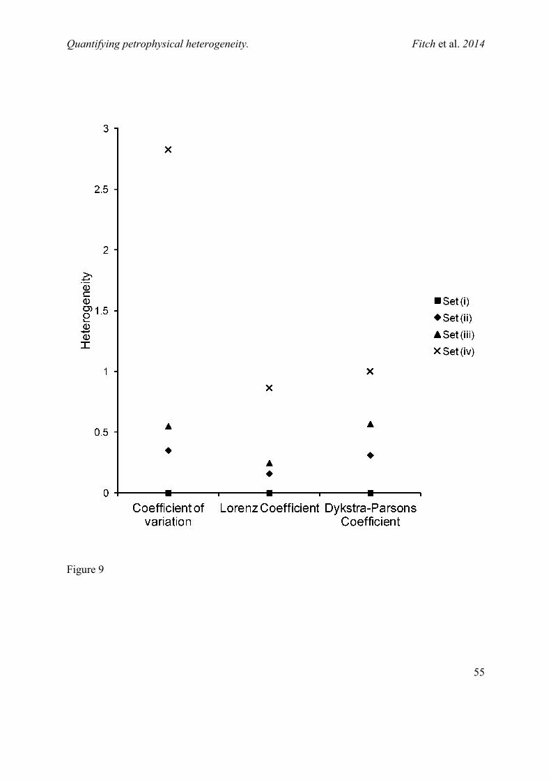
Quantifying petrophysical heterogeneity. Fitch et al. 2014
55
Figure 9

Quantifying petrophysical heterogeneity. Fitch et al. 2014
56
Figure 10

Quantifying petrophysical heterogeneity. Fitch et al. 2014
57
Figure 11

Quantifying petrophysical heterogeneity. Fitch et al. 2014
58
Figure 12

Quantifying petrophysical heterogeneity. Fitch et al. 2014
59
Figure 13

Quantifying petrophysical heterogeneity. Fitch et al. 2014
60
Figure 14

Quantifying petrophysical heterogeneity. Fitch et al. 2014
61
Figure 15
Title: An integrated and quantitative approach to petrophysical heterogeneity.
Authors: Fitch, P. J. R., Lovell, M. A., Davies, S. J., Pritchard, T. and Harvey, P. K.
Highlights
We explore how the term heterogeneity can be defined in earth sciences.
We show that standard statistics can be used to characterise the variability in a dataset.
We investigate the main controls on three static heterogeneity measures.
Four case studies illustrate the application of heterogeneity measures to different data types.