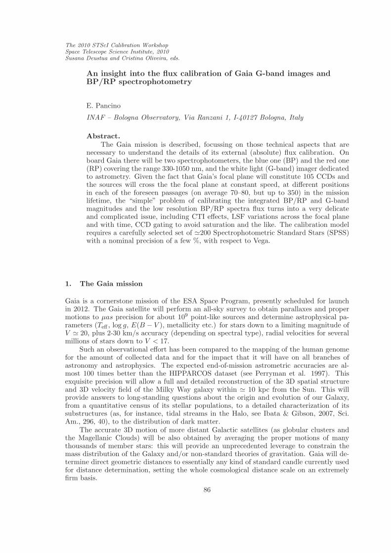
The 2010 STScI Calibration WorkshopSpace Telescope Science Institute, 2010Susana Deustua and Cristina Oliveira, eds.

An insight into the flux calibration of Gaia G-band images andBP/RP spectrophotometry

E. Pancino

INAF – Bologna Observatory, Via Ranzani 1, I-40127 Bologna, Italy

Abstract.The Gaia mission is described, focussing on those technical aspects that are

necessary to understand the details of its external (absolute) flux calibration. Onboard Gaia there will be two spectrophotometers, the blue one (BP) and the red one(RP) covering the range 330-1050 nm, and the white light (G-band) imager dedicatedto astrometry. Given the fact that Gaia’s focal plane will constitute 105 CCDs andthe sources will cross the the focal plane at constant speed, at di!erent positionsin each of the foreseen passages (on average 70–80, but up to 350) in the missionlifetime, the “simple” problem of calibrating the integrated BP/RP and G-bandmagnitudes and the low resolution BP/RP spectra flux turns into a very delicateand complicated issue, including CTI e!ects, LSF variations across the focal planeand with time, CCD gating to avoid saturation and the like. The calibration modelrequires a carefully selected set of !200 Spectrophotometric Standard Stars (SPSS)with a nominal precision of a few %, with respect to Vega.

1. The Gaia mission

Gaia is a cornerstone mission of the ESA Space Program, presently scheduled for launchin 2012. The Gaia satellite will perform an all-sky survey to obtain parallaxes and propermotions to µas precision for about 109 point-like sources and determine astrophysical pa-rameters (Te! , log g, E(B " V ), metallicity etc.) for stars down to a limiting magnitude ofV ! 20, plus 2-30 km/s accuracy (depending on spectral type), radial velocities for severalmillions of stars down to V < 17.

Such an observational e!ort has been compared to the mapping of the human genomefor the amount of collected data and for the impact that it will have on all branches ofastronomy and astrophysics. The expected end-of-mission astrometric accuracies are al-most 100 times better than the HIPPARCOS dataset (see Perryman et al. 1997). Thisexquisite precision will allow a full and detailed reconstruction of the 3D spatial structureand 3D velocity field of the Milky Way galaxy within ! 10 kpc from the Sun. This willprovide answers to long-standing questions about the origin and evolution of our Galaxy,from a quantitative census of its stellar populations, to a detailed characterization of itssubstructures (as, for instance, tidal streams in the Halo, see Ibata & Gibson, 2007, Sci.Am., 296, 40), to the distribution of dark matter.

The accurate 3D motion of more distant Galactic satellites (as globular clusters andthe Magellanic Clouds) will be also obtained by averaging the proper motions of manythousands of member stars: this will provide an unprecedented leverage to constrain themass distribution of the Galaxy and/or non-standard theories of gravitation. Gaia will de-termine direct geometric distances to essentially any kind of standard candle currently usedfor distance determination, setting the whole cosmological distance scale on an extremelyfirm basis.

86

Gaia flux calibration 87

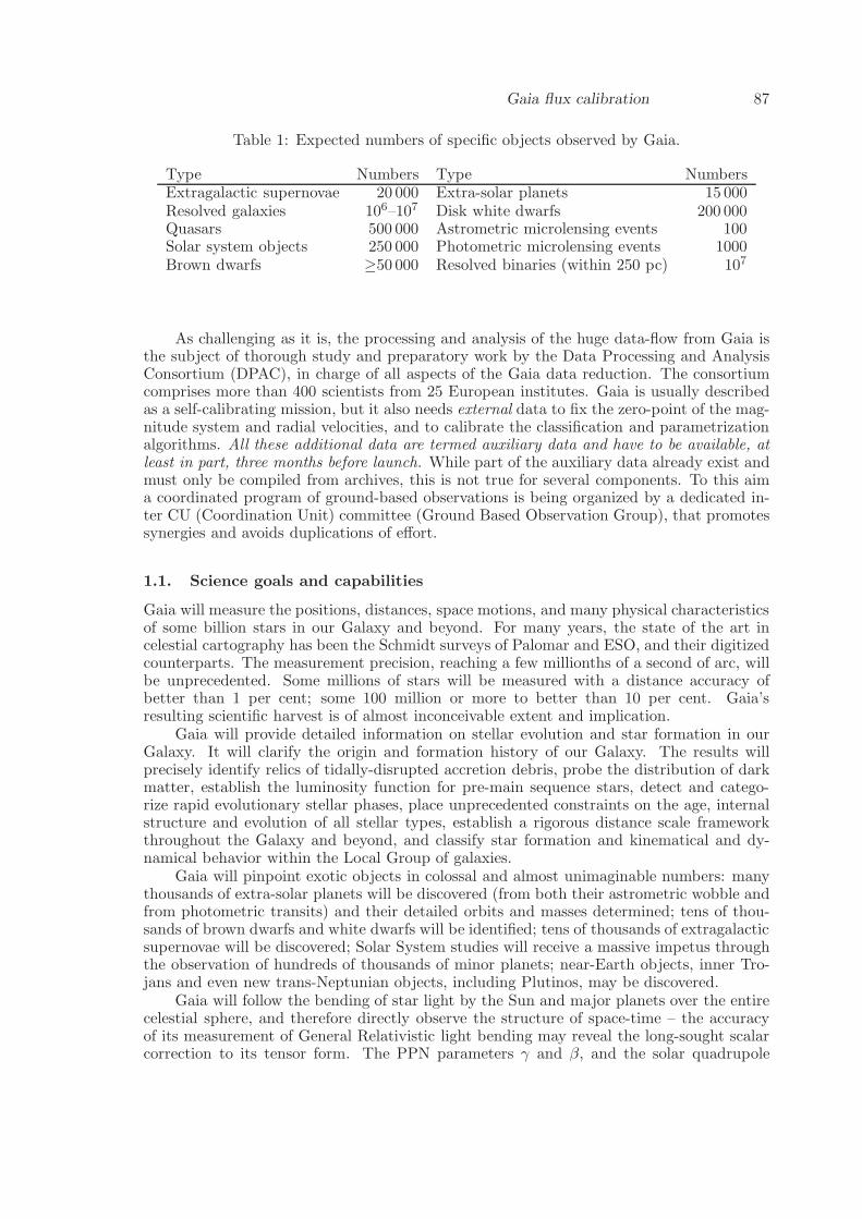
Table 1: Expected numbers of specific objects observed by Gaia.

Type Numbers Type NumbersExtragalactic supernovae 20 000 Extra-solar planets 15 000Resolved galaxies 106–107 Disk white dwarfs 200 000Quasars 500 000 Astrometric microlensing events 100Solar system objects 250 000 Photometric microlensing events 1000Brown dwarfs !50 000 Resolved binaries (within 250 pc) 107

As challenging as it is, the processing and analysis of the huge data-flow from Gaia isthe subject of thorough study and preparatory work by the Data Processing and AnalysisConsortium (DPAC), in charge of all aspects of the Gaia data reduction. The consortiumcomprises more than 400 scientists from 25 European institutes. Gaia is usually describedas a self-calibrating mission, but it also needs external data to fix the zero-point of the mag-nitude system and radial velocities, and to calibrate the classification and parametrizationalgorithms. All these additional data are termed auxiliary data and have to be available, atleast in part, three months before launch. While part of the auxiliary data already exist andmust only be compiled from archives, this is not true for several components. To this aima coordinated program of ground-based observations is being organized by a dedicated in-ter CU (Coordination Unit) committee (Ground Based Observation Group), that promotessynergies and avoids duplications of e!ort.

1.1. Science goals and capabilities

Gaia will measure the positions, distances, space motions, and many physical characteristicsof some billion stars in our Galaxy and beyond. For many years, the state of the art incelestial cartography has been the Schmidt surveys of Palomar and ESO, and their digitizedcounterparts. The measurement precision, reaching a few millionths of a second of arc, willbe unprecedented. Some millions of stars will be measured with a distance accuracy ofbetter than 1 per cent; some 100 million or more to better than 10 per cent. Gaia’sresulting scientific harvest is of almost inconceivable extent and implication.

Gaia will provide detailed information on stellar evolution and star formation in ourGalaxy. It will clarify the origin and formation history of our Galaxy. The results willprecisely identify relics of tidally-disrupted accretion debris, probe the distribution of darkmatter, establish the luminosity function for pre-main sequence stars, detect and catego-rize rapid evolutionary stellar phases, place unprecedented constraints on the age, internalstructure and evolution of all stellar types, establish a rigorous distance scale frameworkthroughout the Galaxy and beyond, and classify star formation and kinematical and dy-namical behavior within the Local Group of galaxies.

Gaia will pinpoint exotic objects in colossal and almost unimaginable numbers: manythousands of extra-solar planets will be discovered (from both their astrometric wobble andfrom photometric transits) and their detailed orbits and masses determined; tens of thou-sands of brown dwarfs and white dwarfs will be identified; tens of thousands of extragalacticsupernovae will be discovered; Solar System studies will receive a massive impetus throughthe observation of hundreds of thousands of minor planets; near-Earth objects, inner Tro-jans and even new trans-Neptunian objects, including Plutinos, may be discovered.

Gaia will follow the bending of star light by the Sun and major planets over the entirecelestial sphere, and therefore directly observe the structure of space-time – the accuracyof its measurement of General Relativistic light bending may reveal the long-sought scalarcorrection to its tensor form. The PPN parameters ! and ", and the solar quadrupole

88 Pancino

Figure 1: The two Gaia telescopes, mounted on a compact torus, point towards two linesof sight separated by 106.5o, and converging on the same focal plane. c!ESA

moment J2, will be determined with unprecedented precision. All this, and more, will beobtained through the accurate measurement of star positions.

We summarize some of the most interesting object classes that will be observed by Gaia,with estimates of the expected total number of objects, in Table 1. For more information onthe Gaia mission: http://www.rssd.esa.int/Gaia. More information for the public on Gaiaand its science capabilities are contained in the Gaia information sheets1. An excellentreview of the science possibilities opened by Gaia can be found in Perryman et al. (1997).

1.2. Launch, timeline and data releases

The first idea for Gaia began circulating in the early 1990, culminating in a proposal for acornerstone mission within ESA’s science program submitted in 1993, and a workshop inCambridge in June 1995. By the time the final catalogue will be released approximatelyin 2020, almost two decades of work will have elapsed between the original concept andmission completion.

Gaia will be launched by a Soyuz carrier (rather than the originally planned Ariane5) in 2012 from French Guyana and will start operating once it reaches its Lissajous orbitaround L2 (the unstable Lagrange point of the Sun and Earth-Moon system), a monthlater. Two ground stations will receive the compressed Gaia data during the 5 years2 ofoperation: Cebreros (Spain) and Perth (Australia). The data will then be transmitted tothe main data centers throughout Europe to allow for data processing. We are presently intechnical development phase C/D, and the hardware is being built, tested and assembled.Software development started in 2006 and is presently producing and testing pipelines with

1http://www.rssd.esa.int/index.php?project=GAIA&page=Info sheets overview.

2If – after careful evaluation – the scientific output of the mission will benefit from an extension of theoperation period, the satellite should be able to gather data for one more year, remaining within the Eartheclipse.

Gaia flux calibration 89

Figure 2: Left: the scanning law of Gaia during main operations; Right: the average numberof passages on the sky, in ecliptic coordinates. c!ESA

the aim of delivering to the astrophysical community a full catalogue and dataset ready forscientific investigation.

Apart from the end-of-mission data release, foreseen around 2020, some intermediatedata releases are foreseen. In particular, there should be one first intermediate releasecovering either the first 6 months or the first year of operation, followed by a second andpossibly a third intermediate release, that are presently being discussed. The data analysiswill proceed in parallel with observations, the major pipelines re-processing all the dataevery 6 months, with secondary cycle pipelines – dedicated to specific tasks – operating ondi!erent timescales. In particular, verified science alerts, based on unexpected variabilityin flux and/or radial velocity, are expected to be released within 24 hours from detection,after an initial period of testing and fine-tuning of the detection algorithms.

1.3. Mission concepts

During its 5-year operational lifetime, the satellite will continuously spin around its axis,with a constant speed of 60 arcsecsec. As a result, over a period of 6 hours, the two astro-metric fields of view will scan across all objects located along the great circle perpendicularto the spin axis (Figure 2, left panel). As a result of the basic angle of 106.5o separatingthe astrometric fields of view on the sky (Figure 1), objects transit the second field of viewwith a delay of 106.5 minutes compared to the first field. Gaia’s spin axis does not point toa fixed direction in space, but is carefully controlled so as to precess slowly on the sky. As aresult, the great circle that is mapped by the two fields of view every 6 hours changes slowlywith time, allowing repeated full sky coverage over the mission lifetime. The best strategy,dictated by thermal stability and power requirements, is to let the spin axis precess (with aperiod of 63 days) around the solar direction with a fixed angle of 45o. The above scanningstrategy, referred to as “revolving scanning”, was successfully adopted during the Hipparcosmission.

Every sky region will be scanned on average 70-80 times, with regions lying at ±45o

from the Ecliptic Poles being scanned on average more often than other locations. Each ofthe Gaia targets will be therefore scanned (within di!erently inclined great circles) from aminimum of approximately 10 times to a maximum of 250 times (Figure 2, right panel).Only point-like sources will be observed, and in some regions of the sky, like the Baade’swindow, ! Centauri or other globular clusters, the star density of the two combined fieldsof view will be of the order of 750 000 or more per square degree, exceeding the storagecapability of the onboard processors, so Gaia will not study in detail these dense areas.

90 Pancino

Figure 3: The 105 on the Gaia focal plane. c!ESA

1.4. Focal plane

Figure 3 shows the focal plane of Gaia, with its 105 CCDs, which are read in TDI (TimeDelay Integration) mode: objects enter the focal plane from the left and cross one CCDin 4 seconds. Apart from some technical CCDs that are of little interest in this context,the first two CCD columns, the Sky Mappers (SM), perform the on-board detection ofpoint-like sources, each of the two columns being able to see only one of the two linesof sight. After the objects are identified and selected, small windows are assigned, whichfollow them in the astrometric field (AF) CCDs where white light (or G-band) images areobtained (Section 1.5.). Immediately following the AF, two additional columns of CCDsgather light from two slitless prism spectrographs, the blue spectrophotometer (BP) andthe red one (RP), which produce dispersed images (Section 1.6.). Finally, objects transit onthe Radial Velocity Spectrometer (RVS) CCDs to produce higher resolution spectra aroundthe Calcium Triplet (CaT) region (Section 1.7.).

1.5. Astrometry

The AF CCDs will provide G-band images, i.e., white light images where the passband isdefined by the telescope optics transmission and the CCDs’ sensitivity, with a very broadcombined passband ranging from 330 to 1050 nm and peaking around 500–600 nm (Fig-ure 4). The objective of Gaia’s astrometric data reduction system is the construction of coremission products: the five standard astrometric parameters, position (!, "), parallax (#),and proper motion (µ!, µ") for all observed stellar objects. The expected end-of-missionprecision in the proper motions is expected to be better than 10 µas for G<10 mag stars,25 µas for G=15 mag, and 300 µas for G=20 mag. For parallaxes, considering a G=12 magstar, we can expect to have distances at better than 0.1% within 250 pc, 1% within 2700 pc,and 10% within 10 kpc.

To reach these end-of-mission precisions, the average 70–80 observations per targetgathered during the 5-year mission duration will have to be combined into a single, global,and self-consistent manner. 40 Gb of telemetry data will first pass through the InitialData Treatment (IDT) which determines the image parameters and centroids, and thenperform object cross-matching. The output forms the so-called One Day Astrometric So-lution (ODAS), together with the satellite attitude and calibration, to sub-milliarcsecondaccuracy. The data are then written to the Main Database.

Gaia flux calibration 91

Figure 4: Left: the passbands of the G-band, BP and RP; Right: a simulated RP dispersedimage, with a red rectangle marking the window assigned for compression and groundtelemetry. c!ESA

The next step is the Astrometric Global Iterative Solution (AGIS) processing. AGISprocesses together the attitude and calibration parameters with the source parameters,refining them in an iterative procedure that stops when the adjustments become su!cientlysmall. As soon as new data come in, on the basis of 6 months cycles, all the data in handare reprocessed together from scratch. This is the only scheme that allows for the quotedprecisions, and it is also the philosophy that justifies Gaia as a self-calibrating mission. Theprimary AGIS cycle will treat only stars that are flagged as single and non-variable (expectedto be around 500 millions), while other kinds of objects will be computed in secondary AGIScycles that utilize the main AGIS solution. Dedicated pipelines for specific kinds of objects(asteroids, slightly extended objects, variable objects and so on) are being put in place toextract the best possible precision. Owing to the large data volume (100 Tb) that Gaiawill produce, and to the iterative nature of the processing, the computing challenges areformidable: AGIS processing alone requires some 1021 FLOPs which translates to runtimesof months on the ESAC computers in Madrid.

1.6. Spectrophotometry

The primary aim of the photometric instrument is mission critical in two respects: (i) tocorrect the measured centroids position in the AF for systematic chromatic e"ects, and (ii)to classify and determine astrophysical characteristics of all objects, such as temperature,gravity, mass, age and chemical composition (in the case of stars).

The BP and RP spectrophotometers are based on a dispersive-prism approach suchthat the incoming light is not focussed in a PSF-like spot, but dispersed along the scandirection in a low-resolution spectrum. The BP operates between 330–680 nm while theRP between 640-1000 nm (Figure 4). Both prisms have appropriate broad-band filters toblock unwanted light. The two dedicated CCD stripes cover the full height of the AF and,therefore, all objects that are imaged in the AF are also imaged in the BP and RP.

The resolution is a function of wavelength, ranging from 4 to 32 nm/pix for BP and 7to 15 nm/pix for RP. The spectral resolution, R=!/"! ranges from 20 to 100 approximately.The dispersers have been designed in such a way that BP and RP spectra are of similar sizes(45 pixels). Window extensions meant to measure the sky background are implemented.To compress the amount of data transmitted to the ground, all the BP and RP spectra– except for the brightest stars – are binned on chip in the across-scan direction, and aretransmitted to the ground as one-dimensional spectra. Figure 4 shows a simulated RPspectrum, unbinned, before windowing, compression, and telemetry.

92 Pancino

Figure 5: Simulated RVS end-of-mission spectra for the extreme cases of 1 single transit(bottom spectrum) and of 350 transits (top spectrum). c!ESA

The final data products will be the end-of-mission (or intermediate releases) of global,combined BP and RP spectra and integrated magnitudes MBP and MRP . Epoch spectrawill be released only for specific classes of objects, such as variable stars and quasars,for example. The internal flux calibration of integrated magnitudes, including the MGmagnitudes as well, is expected at a precision of 0.003 mag for G=13 stars, and for G=20stars goes down to 0.07 mag in MG, 0.3 mag in MBP and MRP . The external calibrationshould be performed with a precision of the order of a few percent (with respect to Vega).

1.7. High-resolution spectroscopy

The primary objective of the RVS is the acquisition of radial velocities, which combined withpositions, proper motions, and parallaxes will provide the means to decipher the kinematicalstate and dynamical history of our Galaxy.

The RVS will provide the radial velocities of about 100–150 million stars up to 17thmagnitude with precisions ranging from 15 km s!1 at the faint end, to 1 km s !1 or betterat the bright end. The spectral resolution, R=!/"! will be 11 500. Radial velocities will beobtained by cross-correlating observed spectra with either a template or a mask. An initialestimate of the source atmospheric parameters will be used to select the most appropriatetemplate or mask. On average, 40 transits will be collected for each object during the 5-yearlifetime of Gaia, since the RVS does not cover the whole width of the Gaia AF (Figure 3). Intotal, we expect to obtain some 5 billion spectra (single transit) for the brightest stars. Theanalysis of this huge dataset will be complicated, not only because of the sheer data volume,but also because the spectroscopic data analysis relies on the multi-epoch astrometric andphotometric data.

The covered wavelength range (847-874 nm) (Figure 5) is a rich domain, centered onthe infrared calcium triplet: it will not only provide radial velocities, but also many stellarand interstellar diagnostics. It has been selected to coincide with the energy distributionpeaks of G and K type stars, which are the most abundant targets. In early type stars, RVSspectra may contain also weak Helium lines and N, although they will be dominated by thePaschen lines. The RVS data will e!ectively complement the astrometric and photometricobservations, improving object classification. For stellar objects, it will provide atmosphericparameters such as e!ective temperature, surface gravity, and individual abundances of key

Gaia flux calibration 93

elements such as Fe, Ca, Mg, Si for millions of stars down to G!12. Also, Di!use InterstellarBands (DIB) around 862 nm will enable the derivation of a 3D map of interstellar reddening.

1.8. The DPAC

ESA will take care of the satellite design, build and testing phases, of launch and operation,and of the data telemetry to the ground, managing the ESAC data center in Madrid, Spain.The data treatment and analysis is the responsibility of the European scientific community.In 2006, the announcement of opportunity opened by ESA was successfully answered by theData Processing and Analysis Consortium (DPAC), a consortium that presently consists ofmore than 400 scientists in Europe (and outside) and more than 25 scientific institutions.

The DPAC executive committee (DPACE) oversees the DPAC activities; work has beenorganized among Coordination Units (CU) in charge of di!erent aspects of data treatment:

• CU1. System Architecture (manager: O’ Mullane), dealing with all aspects ofhardware and software, and coordinating the framework for software development anddata management.

• CU2. Data Simulations (manager: Luri), in charge of the simulators of variousstages of data products, necessary for software development and testing.

• CU3. Core processing (manager: Bastian), developing the main pipelines such asIDT, AGIS and astrometry processing in general.

• CU4. Object Processing (managers: Pourbaix & Tanga), for the processing ofobjects that require special treatment such as minor bodies of the Solar system, forexample.

• CU5. Photometric processing (manager: van Leeuwen), dedicated to the BP,RP, and MG processing and calibration, including image reconstruction, backgroundtreatment, and crowding treatment, among others.

• CU6. Spectroscopic Processing (managers: Katz & Cropper), dedicated to RVSprocessing and radial velocity determination.

• CU7. Variability Processing (managers: Eyer & Evans & Dubath), dedicated toprocessing, classification and parametrization of variable objects.

• CU8. Astrophysical Parameters (managers: Bailer-Jones & Thevenin), develop-ing object classification software and, for each object class, software for the determi-nation of astrophysical parameters.

• CU9. Catalogue Production and Access (to be activated in the near future),responsible for the production of astrophysical catalogues and for the publication ofGaia data to the scientific community.

These are flanked by a few working groups (WG) that deal with aspects that arecommon among the various CUs, such as the GBOG (Ground Based Observerations Group),which coordinates the ground based observations for the external calibration of Gaia) or ofgeneral interest (such as the Radiation task force, serving as the interface between DPACand industry in all matters related to CCD radiation tests).

94 Pancino

2. The flux calibration of Gaia data

Calibrating (spectro)photometry obtained from the usual type of ground based observations(broadband imaging, spectroscopy) is not a trivial task, but the procedures are well known(see e.g., Bessell, 1999) and several scientists have developed sets of standard stars appropri-ated for the more than 200 photometric systems known, and for spectroscopic observations.Generally, magnitudes are calibrated to a standard system with equations in the form

M = m + ZP + !(color) + "(airmass)

where M is the calibrated magnitude in a chosen photometric band, m, the instrumentalmagnitude in the same (or very similar) band, ! is the color term and ", the extinctioncoe!cient due to the Earth’s atmospheric extinction. For the spectra, the instrumentale"ect on the observed spectral energy distribution (SED) is parametrized as

Sobs(#) = R(#) S(#)

where the observed SED, Sobs(#), is the result of the convolution of the “true” SED, S(#),with all the instrumental (transmissivity, quantum e!ciencies) e"ects, which are empiricallydetermined in the form of a response curve, R(#,) through the use of spectrophotometricstandard stars (SPSS). In the case of Gaia, several instrumental e"ects – much more complexthan those usually encountered – redistribute light along the SED of the observed objects.In particular these are: the TDI integration mode, the large focal plane, radiation damageand resulting CTI (charge transfer ine!ciencies), and that the whole instrumental model iswell known only before launch.

2.1. Challenges

The most di!cult Gaia data to calibrate are the BP and RP spectra, requiring a newapproach to the derivation of the calibration model (Section 2.3.) and to the SPSS neededto perform the actual calibration (Section 3.). The large focal plane with its large number ofCCDs makes it so that di"erent observations of the same star will be generally on di"erentCCDs, with di"erent quantum e!ciencies. Also, each CCD is in a di"erent position, withdi"erent optical distortions, optics transmissivity and so on. Therefore, each wavelengthand each position across the focal plane has its (sometimes very di"erent) PSF (point spreadfunction). The TDI and continuous reading mode, combined with the need of compressingthe data before on-ground transmission, make it necessary to translate the full PSF into alinear (compressed into 1D) LSF (line spread function), which of course add complications.In-flight instrument monitoring is foreseen, but never comparable to the full characterizationthat will be performed before launch, so the real instrument – at a certain observation time– will be di"erent from the theoretical one assumed initially, and this di"erence will changewith time.

Radiation damage deserved special mention as it is one of the most important factorsin the time variation of the instrument model. It has particular impact on the BP and RPdispersed images since the objects travel along the BP and RP CCD strips in a directionthat is parallel to the spectral dispersion (wavelength coordinate). Radiation damage causestraps that subtract photons from each passing object at a position corresponding to a certainwavelength. Slow traps release the trapped charges once the object is already passed, whilefast traps can release the charges within the same object, but at a di"erent wavelength.Given the low resolution, one pixel can cover as much as 15–20 nm (depending on thewavelength) and therefore the net e"ect of radiation damage can be to alter significantlythe SED of some spectra. Possible solutions under testing are the equivalent of CCD pre-flashing, the statistical modeling of the traps behavior and the fact that di"erent transitsfor the same object will be a"ected di"erently by CTI e"ects, allowing for a certain degreeof correction through average or median spectra. Finally the PSF/LSF itself is generally

Gaia flux calibration 95

larger than one Gaia pixel in the BP/RP spectra, introducing a large LSF smearing e!ect,i.e., the spread of photons with one particular wavelength into a large range of wavelengths.

In this paper, we will adopt the current Gaia calibration philosophy, where most of theseinstrumental e!ects are taken into account during the so-called internal flux calibration. Alarge number of well behaved stars (internal standards) observed by Gaia will be usedto report all observations to a reference instrument, on the same instrumental flux andwavelength scales. All transits for each object observed by Gaia will be then averaged toproduce one single BP and RP spectrum for each object, with its integrated instrumentalmagnitudes: MG, MBP , and MRP . Only for specific classes of objects will epoch spectraand magnitudes will be released, with variable stars as an obvious example. The meanand epoch spectra will be mostly free from many of the problems examined just above, butthey will still contain residuals due to the imperfect knowledge of the real instrument ateach precise moment of time, and the most significant e!ects are expected to be the LSFsmearing and the CTI e!ects.

In this paradigm, the internal and external flux and wavelength calibrations are treatedas two entirely separate and consecutive pieces of the CU5 photometric pipeline, withdi!erent calibration models. We always start from internally calibrated BP/RP spectraand MG, MBP , and MRP magnitudes, without giving importance to the exact way theyare produced. Presently, two alternative approaches are being considered to maximize theprecision of the global calibration procedure: the first one is a hybrid model that partiallycombines internal and external models (Montegri!o et al. 2010), while the second is theso-called full forwarding model (Carrasco et al. 2010, in preparation), using the samecalibration model for both the internal and external calibration.

2.2. The external calibration teams

Two development units (DU) within CU5 (Photometric processing), are dedicated to theexternal calibration of Gaia photometry. They are DU13: Instrument absolute responsecharacterization: ground-based preparation, coordinated by E. Pancino and DU14, Instru-ment absolute response characterization: definition and application’, coordinated by C. Cac-ciari. They are both based in Bologna, Italy, in collaboration with the Bologna, Barcelona,and Groningen Universities. The actual team members at the time of writing are: G. Al-tavilla, M. Bellazzini, A. Bragaglia, C. Cacciari, J. M. Carrasco, G. Cocozza, L. Federici,F. Figueras, F. Fusi Pecci, C. Jordi, S. Marinoni, P. Montegri!o, E. Pancino, S. Ragaini,E. Rossetti, S. Trager.

2.3. Dispersion Matrix basic definition

If we concentrate now on the mean, internally calibrated BP/RP spectra calibration, wecan write:

Sobs(!I) =N

!

!i=0

T ("i) L!i(!I ! !P ("i)) Strue("i)

where Sobs and Strue are the observed and “true” SEDs respectively, expressed the firstin Gaia pixels !I and the second in wavelength intervals "i corresponding to the actualsampling of the SPSS used in the flux calibration process. T("i) is a combination of allthe instrument and telescope transmissivity functions and aperture, while L is the LSF ata certain "i, centered at the appropriate !I pixel, but of course calculated over the wholewavelength interval from "i=0 to N (the total number of samples in the tabulated SPSSspectrum).

Such an equation can be written in its much simpler matrix form:

Sobs = D " Strue

96 Pancino

Figure 6: Graphical example of a dispersion matrix D, derived with a simulated SPSS setfor the BP (left) and RP (right) instruments, on an arbitrary color scale. c!ESA

where D is called a “Dispersion Matrix”, an object that can be determined if Sobs and Strueare known, i.e., using a well defined set of SPSS observed by Gaia, that also have well knownSED (see below). Once D is properly determined, it can be inverted to convert each mean,internally calibrated BP/RP spectrum3 (Sobs) into a flux calibrated spectrum Strue

Strue = D!1 " Sobs

The main advantage of this approach is that D contains (and therefore corrects em-pirically for) the actual e!ects of LSF smearing – even if the real shape of the LSF is notperfectly known a priori. More than that, the e!ective LSF – as determined with the chosenSPSS set – at each wavelength can be extracted from each column of the matrix. The matrixrows represent instead the e!ective passbands corresponding to each Gaia pixel, includingthe full e!ect of LSF smearing. This peculiar property of the dispersion matrix makes itthe best (and possibly only) solution to the external calibration of Gaia BP/RP spectra.By definition, the dispersion matrix D contains also the actual dispersion function, whichcan be seen in Figure 6 as the curved structure close to the diagonal of the matrix.

Finally, an important by-product of the described calibration model is the absolutewavelength calibration of the BP/RP spectra to a precision of at least a few tenths of aGaia pixel4 (Montegri!o & Bellazzini 2009b), which is automatically performed togetherwith the absolute flux calibration.

There are a few problems in the use of the dispersion matrix as proposed. We willdiscuss in the three following Sections the two most important ones and their proposedsolutions: (1) the matrix is rectangular and its inversion is not so straightforward; (2) thematrix needs a set of independent vectors to be determined in a non-degenerate way (whichalso implies that the set of SPSS must be carefully chosen).

2.4. Smoothing the input SPSS spectra

Clearly, the dispersion matrix is a rectangular matrix: the Gaia observations have a smallernumber of samples (pixels) than the SPSS spectra used to build their calibration model(wavelength sampling). Inverting a rectangular matrix is a non-trivial task so if we want

3Incidentally, for some object classes that need it, such as variable stars, single transits – the so called epochspectra – will be published. The described calibration model can be applied also to single epoch spectra oncethey have been internally calibrated, i.e., reported to a common, instrumental scale of flux and wavelength.

4This first estimate of the wavelength zero point and scale precision is based on a slightly outdated calibrationmodel formulation, an therefore has to be considered just as an upper limit to a more realistic uncertainty(Montegri!o, 2010, private communication.

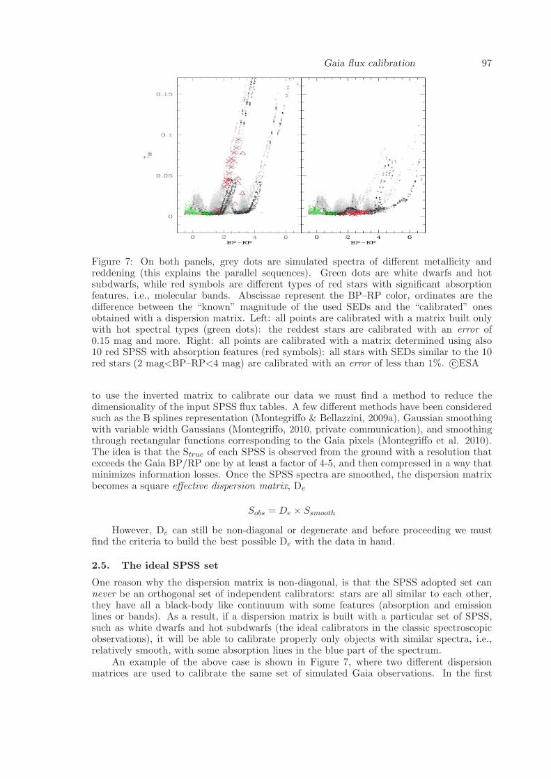
Gaia flux calibration 97

Figure 7: On both panels, grey dots are simulated spectra of di!erent metallicity andreddening (this explains the parallel sequences). Green dots are white dwarfs and hotsubdwarfs, while red symbols are di!erent types of red stars with significant absorptionfeatures, i.e., molecular bands. Abscissae represent the BP–RP color, ordinates are thedi!erence between the “known” magnitude of the used SEDs and the “calibrated” onesobtained with a dispersion matrix. Left: all points are calibrated with a matrix built onlywith hot spectral types (green dots): the reddest stars are calibrated with an error of0.15 mag and more. Right: all points are calibrated with a matrix determined using also10 red SPSS with absorption features (red symbols): all stars with SEDs similar to the 10red stars (2 mag<BP–RP<4 mag) are calibrated with an error of less than 1%. c!ESA

to use the inverted matrix to calibrate our data we must find a method to reduce thedimensionality of the input SPSS flux tables. A few di!erent methods have been consideredsuch as the B splines representation (Montegri!o & Bellazzini, 2009a), Gaussian smoothingwith variable width Gaussians (Montegri!o, 2010, private communication), and smoothingthrough rectangular functions corresponding to the Gaia pixels (Montegri!o et al. 2010).The idea is that the Strue of each SPSS is observed from the ground with a resolution thatexceeds the Gaia BP/RP one by at least a factor of 4-5, and then compressed in a way thatminimizes information losses. Once the SPSS spectra are smoothed, the dispersion matrixbecomes a square e!ective dispersion matrix, De

Sobs = De " Ssmooth

However, De can still be non-diagonal or degenerate and before proceeding we mustfind the criteria to build the best possible De with the data in hand.

2.5. The ideal SPSS set

One reason why the dispersion matrix is non-diagonal, is that the SPSS adopted set cannever be an orthogonal set of independent calibrators: stars are all similar to each other,they have all a black-body like continuum with some features (absorption and emissionlines or bands). As a result, if a dispersion matrix is built with a particular set of SPSS,such as white dwarfs and hot subdwarfs (the ideal calibrators in the classic spectroscopicobservations), it will be able to calibrate properly only objects with similar spectra, i.e.,relatively smooth, with some absorption lines in the blue part of the spectrum.

An example of the above case is shown in Figure 7, where two di!erent dispersionmatrices are used to calibrate the same set of simulated Gaia observations. In the first

98 Pancino

Figure 8: Left: example of a degenerate dispersion matrix, De (which is square, see text),where the diagonal is drowned into noise-like patterns due to the degenerate (non indepen-dent) set of SPSS used to construct it. Right: an example of a diagonal dispersion matrix,obtained with an appropriate SPSS set and with the use of a nominal dispersion matrix tofurther reduce degeneracy (see text). c!ESA

case (left panel of Figure 7), a dispersion matrix is built using only white dwarfs and hotsubdwarfs, with a minority of solar type stars, and it can clearly be seen that red stars withdeep absorption bands are calibrated with an error of 0.15 mag at least, failing the specifiedrequirements. In the second case (right panel of Figure 7), a small number (10) of red starswith deep absorption bands are included in the SPSS set used to build a second dispersionmatrix. The second dispersion matrix is able to calibrate all red stars with absorptionfeatures to better than 1%, exceeding the requirements.

This example shows the importance of spectral features in the SPSS set used in con-struction of the dispersion matrix. Hot stars have prominent absorption lines in the blue,but no features in the red. The addition of a few red stars with absorption bands “trains” thematrix in the calibration of stars with features in the red (e!ectively reducing degeneracy).Similarly, problems are encountered in the calibration of emission line objects (peculiar hotstars and quasars, for example). But it is quite di"cult to include these objects into theSPSS set since they are often variable.

Even if several types of objects are included when determining the dispersion matrix,other e!ects can have a large impact on the degeneracy, such as edge e!ects. For thesereasons, the accurate choice of the SPSS set is crucial, but does not solve the problem ofdegeneracy once and for all.

2.6. Nominal dispersion matrix

To further reduce degeneracy of the e!ective dispersion matrix De, we can use other con-straints such as the fact that we know most aspects of the instrument from pre-launchcharacterization. These include the quantum e"ciency of the CCDs, the optical layout andtransmissivity, the nominal LSF at various positions along the focal plane and at di!erentwavelengths, the nominal dispersion function and its variation along the focal plane. Theslow change of these with time can also be monitored to a certain extent, and included inthe models.

We can therefore separate the dispersion matrix in a part that is theoretically modeledbased on pre-launch instrument description and on its (partially reconstructed) variationwith time, which we call Dn or nominal dispersion matrix, and in a part that is completely

Gaia flux calibration 99

unknown, which can be considered as a correction matrix K, made of the residual correctionsafter the nominal model is taken into account (Montegri!o et al. 2010)

De = K ! Dn

The nominal matrix will be clean: diagonal and non-degenerate (see Figure 8). Thecorrection matrix will be partially degenerate, but all signal that lies far away from thediagonal can be safely considered spurious (the system varies in a continuous way, thecorrections must be “small” compared to the nominal system), and the part of the correctionmatrix close to its diagonal can be easily modeled.

To summarize all the previously defined steps, once an appropriate SPSS set is chosen,the calibration model becomes

Sobs = De ! Ssmooth = K ! Dn ! Ssmooth

and the matrices involved can be easily inverted to calibrate all Gaia observations sincethey are all square and (almost completely) diagonal.

2.7. Integrated magnitudes

A classical approach can be adopted for the absolute flux calibration of integrated MG,MBP , and MRP magnitudes (Ragaini et al., 2009a,b) in the form

M = m + ZP

where M is the calibrated magnitude, m the internally calibrated one observed by Gaia,and ZP is the required zero-point. No significant color term appears necessary.

However, if we consider that an integrated magnitude M is the convolution of thespectral distribution Strue and the e!ective passband B, we can calibrate integrated magni-tudes with the same approach adopted for BP/RP spectra, with a much more homogeneousprocedure from the point of view of pipeline code writing

M = Strue ! B

Since generally the passband B is sampled di!erently than the SPSS flux table Strue,we must smooth to one or both Strue and B. Similarly to the case of BP/RP spectra, wecan split B into two components

B = K ! ! Bn

where K’ is a correction vector, made of the actual residuals to a theoretically known – ornominal – e!ective passband Bn, known before launch and slowly varying with time due toseveral causes, the most important one being the decrease in CCD quantum e"ciency due toradiation damage. With this kind of treatment, the problem becomes a simple least squarefitting problem to derive the unknown K’ vector (Ragaini et al., 2010, in preparation).

2.8. RVS calibration

The possibility of flux calibrating the RVS spectra has been so far considered a secondaryproblem, since both radial velocities and astrophysical parameters can be derived withoutthe need of an absolute flux scale attached to the spectra. A preliminary set of considerations(Trager, 2010) shows that in principle the SPSS grid for the calibration of Gaia G-band andBP/RP data, that is presently under construction, should be su"ciently sampled to ensurea flux calibration of RVS spectra as well. We expect the topic to be further explored byCU6 (Spectroscopic processing) in the near future, but we will not consider RVS spectraflux calibration in this paper.

100 Pancino

Figure 9: The RA/Dec distribution of Primary (left) and Secondary SPSS candidates(right). The three Pillars are marked in red in the left panel, while the targets close tothe ecliptic poles are marked in green in the right panel. The size of symbols is inverselyproportional to the SPSS magnitude. The two stripes at ±45 deg from the Ecliptic Polesare marked in both panels. c!ESA

3. The Gaia grid of spectrophotometric standard stars

From the above discussion, it is clear that the Gaia SPSS grid has to be chosen with greatcare. The Gaia SPSS, or better their reference flux tables (corresponding to Strue in theprevious Sections) should conform to the following general requirements (van Leaven et al.2010):

• Resolution R=!/"! " 1000, i.e., they should over sample the Gaia BP/RP resolutionby a factor of 4–5 at least;

• Wavelength coverage: 330–1050 nm;

• Typical uncertainty in the absolute flux scale, with respect to the assumed calibrationof Vega, of a few percent, excluding small troubled areas in the spectral range (telluricbands residuals, extreme red and blue edges), where it can be somewhat worse.

The total number of SPSS in the Gaia grid should be of the order of 200–300 stars,including a variety of spectral types. Clearly, no such large and homogeneous datasetexists in the literature yet5. It is therefore necessary to build the Gaia SPSS grid withnew, dedicated observations. We describe the characteristics of the Gaia SPSS and of thededicated observing campaigns in the following sections.

3.1. SPSS Candidates

We have followed a two step approach (Bellazzini et al. 2007) that first creates a setof Primary SPSS, i.e., well known SPSS that are calibrated on the three Pillars of theCALSPEC6 set, described in Bohlin et al. (1995,2007), and tied to the Vega flux calibration

5The CALSPEC database (Bohlin, 2007) is not large enough for our purpose, especially considering the strictcriteria described below. Its extension to more than 100 SPSS is eagerly awaited, but still not available tothe public.

6http://www.stsci.edu/hst/observatory/cdbs/calspec.html

Gaia flux calibration 101

Figure 10: The preliminary reductions (no telluric correction, only TNG (TelescopioNazionale Galileo) observations, library extinction curve, and so on) of star GD 71 (toppanel) are compared with the CALSPEC spectrum (bottom panel). Prominent telluricfeatures are marked in both panels. Except for the spectral edges – which will need to bereconstructed with the use of models – the main body of the spectrum is always close tothe CALSPEC one within 1% or better. c!ESA

by Bohlin & Gilliland (2004) and Bohlin et al. (2007). An example of the kind of spectraobtained for Pillar GD 71 (with DoLoRes at the TNG is shown on Figure 10. The PrimarySPSS will constitute the ground-based calibrators of the actual Gaia grid, and need toconform to the following requirements (van Leeuwen 2010):

• Primary SPSS have spectra as featureless as possible;

• Primary SPSS shall be validated against variability;

• Primary SPSS have already well known SEDs;

• The magnitude of each Primary SPS results in S/N"100 per pixel over most of thewavelength range when observed from the ground with 2m class telescopes;

• The location of Primary SPSS is in non crowded areas of the sky;

• Primary SPSS cover a range of RA and Dec to ensure all-year-round ground basedobservations from both hemispheres.

The Primary SPSS candidates set is described in more detail in Altavilla et al. (2008),and some of the most important sources for Primary candidates are the CALSPEC grid,Oke (1990), Hamuy et al. (1992,1994), Stritzinger et al. (2005) and others. The actual GaiaSPSS grid, or Secondary SPSS, conforms to a di!erent set of requirements (van Leeuwen2010):

• Secondary SPSS have spectra as featureless as possible (but see below for exceptions);

• Secondary SPSS shall be validated against variability;

102 Pancino

Figure 11: Left: example of a short-term variability curve for a constant SPSS candidate.Right: example of a short-term variability curve for a variable SPSS candidate. c!ESA

• The magnitude and sky location (i.e., number of useful, clean transits, see Carrascoet al. 2006, 2007) of Secondary SPSS grants a resulting S/N"100 per sample overmost of the wavelength range when observed by Gaia (end of mission);

• Secondary SPSS cover a range of spectral types and spectral shapes, as needed toensure the best possible calibration of all kinds of objects observed by Gaia.

As already mentioned, Secondary SPSS will be mostly hot and featureless stars butwill include a small number of selected spectral types, to ensure that the calibration modelcan work on all object types. More details on Secondary SPSS can be found in Altavillaet al. (2010), including a long list of literature catalogs and online databases from whichthe candidates are extracted. Clearly, all the Primary SPSS that, at the end of the datareductions, will satisfy also the criteria for Secondary SPSS, will be included in the GaiaSPSS grid.

Additionally, special members of the Secondary SPSS candidates are: (1) a few selectedSPSS around the Ecliptic Poles, two regions of the sky that will be repeatedly observed byGaia, in the first two weeks after reaching its orbit in L2, for calibration purposes; (2)a few M stars with deep absorption features in the red; (3) a few SDSS stars that havebeen observed in the SEGUE sample (Yanny et al., 2009), since the SEGUE sample hasthe potential of being extremely useful in the Gaia flux calibration (Bellazzini et al. 2010),both internal (relative) and external (absolute); (4) a few well known SPSS that are amongthe targets of the ACCESS mission (Kaiser et al., 2010), dedicated to the absolute fluxmeasurement of a few stars besides Vega.

3.2. Observation strategy and campaigns

A basic consideration when starting the observations of such a large campaign, is thatthe traditional spectrophotometry techniques require too much observing time: each SPSSshould be spectroscopically observed in perfect photometric conditions, ideally more thanonce. No TAC (Time Allocation Committee) would grant such a large amount of observingtime to a proposal that does not contain any cutting edge science in it.

We therefore chose (Bellazzini et al. 2007) to split the problem into two parts: (1)spectra are taken in good sky conditions, but not necessarily perfectly photometric; they

Gaia flux calibration 103

are calibrated with the help of a Pillar or Primary SPSS thus recovering the correct spectralshape; (2) absolute photometry in the B, V, and R (sometimes I) Johnson-Cousins bandsis taken in photometric sky conditions and used to fix the spectral zero-point by means ofsynthetic photometry. This is motivated by the fact that absolute photometric night pointsare faster to obtain than spectra. A subset of SPSS candidates will be spectroscopicallyobserved in photometric sky conditions, to check the whole procedure.

Besides the Main Campaign just described, it is necessary to monitor candidate SPSSfor constancy (Auxiliary Campaign), since very few of them have systematically been mon-itored in the literature, and there are illustrious examples of stars that showed unexpectedvariability (Landolt & Uomoto, 2007). An example of a di!erent kind of problem, thatcould greatly benefit from good quality dedicated imaging, is star HZ 43. It was initiallychosen by Bohlin et al. (1995) to be one of the Pillars, and later rejected because of anoptical companion lying 3” away, only visible in the V band, that made it useless as anSPSS from the ground.

Most of our SPSS candidates are WDs close to the instability strip, and, which, some-times have poorly known magnitudes, so it is necessary to monitor them for short-termvariability on scales of 1–2 hours (Figure 11). Binary systems are frequent and can befound at all spectral types, so we also monitor all our candidates for long-term variability(3 years) collecting approximately 4 night points per year. These two monitoring campaignsrely on relative photometry (using stars in the field of view) to derive variability curves. AnSPSS candidate is considered constant if it does not vary with an amplitude larger than afew milli-mags.

The facilities that are being used for the two observing campaigns are (Federici et al.,2007, Altavilla et al. 2010):

• EFOSC@NTT (New Technology Telescope) La Silla, Chile (primarily Main cam-paign);

• ROSS@REM (Rapid Eye Munt Telescope) , La Silla, Chile (primarily Auxiliary cam-paign);

• LARUCA@1.5m, San Pedro Martir, Mexico (primarily Auxiliary campaign and abso-lute photometry);

• BFOSC@Cassini, Loiano, Italy (primarily Auxiliary campaign);

• CAFOS@2.2m, Calar Alto, Spain (primarily Main campaign);

• DoLoRes@TNG (Telescopio Nazionale Galileo), La Palma, Spain (primarily Maincampaign);

Observations started in the second half of 2006, comprising more than 35 acceptedproposals. We have been awarded a total of 230 observing nights approximately, at therate of 33 per semester. More than 50% of this time resulted in at least partially usefuldata. Given the large number of facilities involved, and of di!erent observers, it has becomenecessary to establish strict observing protocols (Pancino et al. 2008,2009). The campaignsare now more than 50% complete, with the spectroscopy observations 75% complete, andwe expect to complete all our observing campaigns around 2013.

3.3. Data reduction and analysis

The large amount of data collected needs to be reduced and analyzed with the max-imum possible precision and homogeneity. An initial set of data is collected for eachCCD/instrument/telescope combination and an Instrument Familiarization Plan (IFP) is

104 Pancino

Figure 12: Example of the 2nd order contamination in the DoLoRes grism LR-R, and of itscorrection for stars HZ 44 and G 146–76. The solid black curves are the corrected spectrawhile the red curves are the contaminating light coming from the 2nd order dispersed bluelight. c!ESA

conducted, to derive shutter times, linearity, calibration frames and lamps stability, photo-metric distortions, 2nd order contamination of spectra (Figure 12), and so on. This plan isnow almost complete, and the protocols are presently being finalized and written.

The data reduction is regulated by strict data reduction protocols, that are presentlybeing finalized. While the data reduction methods are fairly standard, care must be takenin considering the characteristics of each instrument, as determined during the IFP, to ex-tract the highest possible quality from each instrument. Semi-automatic quality check (QC)criteria are defined for each kind of observation (minimum & maximum S/N, seeing androundness requirements of images, presence of bad columns, companions, and so on). Onlyframes that pass the QC are reduced. For imaging, we term “data reduction” the removalof the instrument characteristics (dark, bias, flat-field, fringing), QC, and the measurementof aperture photometry with SExtractor (Bertin & Arnouts, 1996). The data products are2D reduced images and aperture magnitude catalogues. For spectroscopy, we term “datareduction” the removal of instrumental features (dark, bias, flat-field, illumination correc-tion, wavelength calibration, 2nd order contamination correction, relative flux calibration,telluric features removal), followed by QC and spectra extraction. The data products are2D reduced frames, 1D extracted and wavelength calibrated spectra, 1D flux calibratedspectra, 1D telluric absorption corrected spectra.

The data reduction procedures are well advanced for photometry (almost half of thedata reduced) and have just started for spectra (10% of the data reduced) at the momentof writing.

The data analysis is presently in the design and testing phases. The study of short-term variability curves is proceeding (10% of the data analyzed, see Figure 11). Absolutephotometry and relative spectroscopy procedures are being refined: for example, preliminaryend-to-end reduction of photometric imaging nights have been performed for TNG and NTTobservations, to allow us to identify those nights that were actually photometric and didnot need to be repeated. Preliminary extinction curves have been determined for TNG andCAHA (Centro Astrono Hispano Aleman) (spectroscopic observations, allowing us to see

Gaia flux calibration 105

Figure 13: The simple browsing interface of the Wiki-Bo local SPSS archive. This snapshotrefers to the raw data archive, a similar web page exists for data products. c!ESA

that extinction varies in a grey manner (within a few percent) even in the case of someCalima (desert dust) in the sky over La Palma.

The final data products for the Auxiliary campaign will be relative magnitudes andlightcurves for all the monitored candidate SPSS; for the Main campaign, absolute mag-nitudes and errors will be released together with their uncertainties and flux tables (Fig-ure 10) in the form (!(nm),F!(photons s!1 m!2 nm!1)). Possibly, also other intermediatedata products will be released (see above).

3.4. Data availability

All the data SPSS ground based observations, along with the collected literature informationand measurements, are stored in the CU5-DU13 local Wiki pages in Bologna (Wiki-Bo)7.Wiki-Bo also contains all our technical documentation, internal reports, observation statusand data products, along with literature references and sources, observing proposals andthe like. The raw and reduced data products are stored in a local archive8 for internalpurposes (Figure 13).

In the future, when CU9 begins (Catalogue production and access), it is foreseen thatall the ground-based data used for the calibration of Gaia data (radial velocity standards,SPSS, spectral libraries, Ecliptic pole observations, observations of Gaia itself from theground, and so on) will be published as well, although no decision on the format and typeof data products has been made yet.

4. Conclusions

The Gaia mission and its data reduction is a challenging enterprise, carried out by ESAand the European scientific community. As an example of the DPAC (Data Processingand Analysis Consortium) tasks, I have briefly summarized the problem of the external(absolute) flux calibration of spectrophotometric Gaia data, and more specifically of theBP/RP low resolution spectra and the integrated G-band and BP/RP magnitudes. Aninnovative calibration model is presently under study and testing, and a large (" 200#300)

7http://yoda.bo.astro.it/wiki, guest username and password can be obtained from E. Pancino.

8http://spss.bo.astro.it, guest username and password can be obtained from E. Pancino.

106 Pancino

grid of SPSS with 1–3% flux calibration with respect to Vega is being built from multi-siteground-based observations.

But once the Gaia data will become available, a greater challenge will have to be faced:the impact in almost all fields of astrophysics require that the scientific community (and notonly the European one) be adequately prepared to extract the most scientific output fromthe data. The training of a new generation of scientists, and the collection of complementarydata, necessary to answer key questions when combined with Gaia data, should start now.The challenge requires that large groups of scientists get e!ciently organized and ready tocollaborate on large and comprehensive datasets.

References

Altavilla, G., Bellazzini, M., Pancino, E., Bragaglia, A., Cacciari, C, Diolaiti, E., Federici,L., Montegri"o, P., Rossetti, E., 2008, “Primary standards for the establishment ofthe Gaia grid of SPSS. Selection criteria and a list of candidates”, Gaia technicalreport GAIA-C5-TN-OABO-GA-001

Altavilla, G., Bragaglia, Pancino, E., Bellazzini, M., A., Cacciari, C, Federici, L., Ragaini,S., 2010, “Secondary standards for the establishment of the Gaia grid of SPSS. Selec-tion criteria and a list of candidates”, Gaia technical report GAIA-C5-TN-OABO-GA-003

Bellazzini, M., Bragaglia, A., Federici, L., Diolaiti, E., Cacciari, C., Pancino, E., 2006,“Absolute calibration of Gaia photometric data. I. General considerations and re-quirements”, Gaia technical report GAIA-C5-TN-OABO-MBZ-001

Bellazzini, M., Altavilla, G., Cacciari, C., 2010, “Notes on the possible use of SEGUEspectrophotometry for the absolute photometric calibration of Gaia”, Gaia technicalreport GAIA-C5-TN-OABO-MBZ-002

Bertin, E., & Arnouts, S. 1996, A&AS, 117, 393

Bessell, M. S. 1999, PASP, 111, 1426

Bohlin, R. C., Colina, L., & Finley, D. S. 1995, AJ, 110, 1316

Bohlin, R. C. 2007, PASP, The Future of Photometric, Spectrophotometric and PolarimetricStandardization, 364, 315

Carrasco, J. M., Jordi, C., Figueras, F., Anglada-Escude, G., 2006, “Towards a selectionof standard stars for absolute flux calibration. Signal-To-Noise ratios for BP/RPspectra and crowding due to FoV overlapping”, Gaia technical report GAIA-C5-TN-UB-JMC-002

Carrasco, J. M., Jordi, C., Lopez-Marti, B., Figueras, F., Anglada-Escude, G., Amores,E. B., 2007, “Revolving phase e!ect to FoV overlapping and its application to Pri-mary SPSS”, Gaia technical report GAIA-C5-TN-UB-JMC-002

Carrasco, J. M. et al., 2010, in preparation, “Design of the experiment to test BP/RP fullforwarding model”, Gaia technical report GAIA-C5-TN-UB-JMC-011

Hamuy, M., Suntze", N. B., Heathcote, S. R., Walker, A. R., Gigoux, P., & Phillips, M. M.1994, PASP, 106, 566

Hamuy, M., Walker, A. R., Suntze", N. B., Gigoux, P., Heathcote, S. R., & Phillips, M. M.1992, PASP, 104, 533

Kaiser, M. E., et al. 2010, arXiv:1001.3925

Landolt, A. U., & Uomoto, A. K. 2007, AJ, 133, 768

Montegri"o, P., & Bellazzini, M. 2009a, “A model for the absolute photometric calibrationof Gaia BP and RP spectra. III. A full in-flight calibration of the model parameters”,Gaia technical report GAIA-C5-TN-OABO-PMN-003

Gaia flux calibration 107

Montegri!o, P., & Bellazzini, M. 2009b, “Quantitative estimate of the uncertainty on thewavelength calibration as derived from the absolute calibration process”, Gaia techni-cal report GAIA-C5-TN-OABO-PMN-004

Montegri!o, P., et al., 2010, in preparation “Planning an experiment on source and instru-ment update XP processing”, Gaia technical report GAIA-C5-TN-OABO-PMN-005

Oke, J. B. 1990, AJ, 99, 1621

Perryman, M. A. C., Lindegren, L., & Turon, C. 1997, Hipparcos - Venice ’97, 402, 743

Pancino, E., Altavilla, G., Bellazzini, M., Marinoni, S., Bragaglia, A., Federici, L., Cacciari,C., 2008, “Protocol for ground based observations of SPSS. I. Instrument familiar-ization tests”, Gaia technical report GAIA-C5-TN-OABO-EP-001

Pancino, E., Altavilla, G., Carrasco, J. M., M, Monguio, Marinoni, S., Rossetti, E., Bellazz-ini, M., Bragaglia, A., Federici, L., Schuster, W.., 2009, “Protocol for ground basedobservations of SPSS. II. Variability searches and absolute photometry campaigns”,Gaia technical report GAIA-C5-TN-OABO-EP-003

Ragaini, S., Bellazzini, M., Montegri!o, P., Cacciari, C., 2009a, “Absolute calibration of Gand integrated BP and RP fluxes”, Gaia technical report GAIA-C5-TN-OABO-SR-001

Ragaini, S., Montegri!o, P., Bellazzini, M., Cacciari, C., 2009b, “Absolute calibration of Gand integrated BP and RP fluxes: test and limits of a simple model”, Gaia technicalreport GAIA-C5-TN-OABO-SR-002

Ragaini, S., et al., 2010, in preparation “Absolute calibration of G and integrated BP andRP fluxes: a new model”, Gaia technical report GAIA-C5-TN-OABO-SR-003

Stritzinger, M., Suntze!, N. B., Hamuy, M., Challis, P., Demarco, R., Germany, L., &Soderberg, A. M. 2005, PASP, 117, 810

Trager, S., 2010, “Spectrophotometric calibration of RVS using CU5-DU13 flux calibrationtables”, Gaia technical report GAIA-C5-TN-UG-ST-002

van Leeuwen, F. & the CU5 DU managers, 2010, “CU5 software requirements specifica-tions”, Gaia technical report GAIA-C5-SP-IOA-FVL-014

Yanny, B., et al. 2009, AJ, 137, 4377