An improved energy management methodology for the mining ...

An improved energy management methodology for the mining industry

by

Michelle

Levesque

A thesis submitted in partial fulfillment of the requirements for the degree of

Doctor of Philosophy (PhD) in Natural Resources Engineering

The Faculty of Graduate Studies Laurentian University

Sudbury, Ontario, Canada

© Michelle Levesque, 2015

ii

THESIS DEFENCE COMMITTEE/COMITÉ DE SOUTENANCE DE THÈSE

Laurentian Université/Université Laurentienne

Faculty of Graduate Studies/Faculté des études supérieures

Title of Thesis

Titre de la thèse An improved energy management methodology for the mining industry

Name of Candidate

Nom du candidat Levesque, Michelle

Degree

Diplôme Doctor of Philosophy

Department/Program Date of Defence September 10, 2015

Département/Programme Natural Resources Engineering Date de la soutenance

APPROVED/APPROUVÉ

Thesis Examiners/Examinateurs de thèse:

Dr. Dean Millar

(Supervisor/Directeur(trice) de thèse)

Dr. Marty Hudyma

(Committee member/Membre du comité)

Dr. Helen Shang

(Committee member/Membre du comité)

Approved for the Faculty of Graduate Studies

Dr. Monica Carvalho Approuvé pour la Faculté des études supérieures

(Committee member/Membre du comité) Dr. David Lesbarrères

Monsieur David Lesbarrères

Dr. John Nyboer Acting Dean, Faculty of Graduate Studies

(External Examiner/Examinateur externe) Doyen intérimaire, Faculté des études supérieures

Dr. Ubi Wichoski

(Internal Examiner/Examinateur interne)

ACCESSIBILITY CLAUSE AND PERMISSION TO USE

I, Michelle Levesque, hereby grant to Laurentian University and/or its agents the non-exclusive license to archive

and make accessible my thesis, dissertation, or project report in whole or in part in all forms of media, now or for the

duration of my copyright ownership. I retain all other ownership rights to the copyright of the thesis, dissertation or

project report. I also reserve the right to use in future works (such as articles or books) all or part of this thesis,

dissertation, or project report. I further agree that permission for copying of this thesis in any manner, in whole or in

part, for scholarly purposes may be granted by the professor or professors who supervised my thesis work or, in their

absence, by the Head of the Department in which my thesis work was done. It is understood that any copying or

publication or use of this thesis or parts thereof for financial gain shall not be allowed without my written

permission. It is also understood that this copy is being made available in this form by the authority of the copyright

owner solely for the purpose of private study and research and may not be copied or reproduced except as permitted

by the copyright laws without written authority from the copyright owner.

iii

Abstract

The focus for this work was the development of an improved energy management methodology

tailored for the mining sector. Motivation for this research was driven by perception of slow

progress in adoption of energy management practices to improve energy performance within the

mining sector. Energy audits conducted for an underground mine, a mineral processing facility,

and a pyrometallurgical process were reviewed and recommendations for improved data

gathering, reporting and interpretation were identified.

An obstacle for conducting energy audits in mines without extensive sub-metering is a lack of

disaggregated data indicating end use. Thus a novel method was developed using signal

processing techniques to disaggregate the end-use electricity consumption, exemplified through

isolation of a mine hoist signal from the main electricity meter data. Further refinements to the

method may lead to its widespread adoption, which may lower energy auditing costs via a

reduced number of meters and infrastructure, as well as lower data storage requirements.

Mine ventilation systems correspond to the largest energy demand center for underground mines.

Thus a detailed analysis ensued with the development of a techno-economic model that could be

used to assess various fan and duct options. Furthermore, the need for a standardized

methodology for determination of duct friction factors from ventilation surveys was proposed,

which included a method to verify the validity of the resulting value from asperity height

measurements. A method was also suggested for determination of leakage and duct friction

factor values from ventilation survey data.

Dissemination of best practice is a strategy that could be employed to improve energy

performance throughout the mining sector, thus a Best Practice database was developed to

iv

improve communication and provide a standardized reporting framework for sharing of energy

conservation initiatives.

Demonstration of continuous improvement is an underpinning element of the ISO 50001 energy

management standard but as mines extract ore from deeper levels energy use increases. Thus

ensued the development of a benchmarking metric, with the use of appropriate support variables

that included mine depth, production, and climate data, that demonstrated the benefit of

implemented energy conservation measures for an underground mine.

The development of an ultimate energy management methodology for all stages of mineral

processing from ‘Mine to Bullion’ is beyond the scope of this work. However, this research has

resulted in several recommendations for improvement and identified areas for further

improvements.

v

Keywords

energy management; energy audits; mining industry; energy reporting; energy benchmarking;

auxiliary mine ventilation; dissemination of best practice energy management; signal processing;

electricity disaggregation;

vi

Co-Authorship Statement

The following includes a list of publications included within the thesis with the nature and scope

of work from co-authors.

LEVESQUE, M.Y. and MILLAR, D.L., 2015. The link between operational practices and

specific energy consumption in metal ore milling plants – Ontario experiences. Minerals

Engineering, 71(0), pp. 146-158.

Levesque, M.Y. was responsible for conducting the data analysis and interpretation of the

results whereas Millar, D.L. reviewed the work and participated in discussions that

allowed the work to progress.

LEVESQUE, M., MILLAR, D. and PARASZCZAK, J., 2014. Energy and mining – the home

truths. Journal of Cleaner Production, 84(0), pp. 233-255.

Data collection and analysis was conducted by Levesque, M., whereas Millar, D. and

Paraszczak, J. reviewed the work and provided useful discussions and comments to

improve the manuscript content and structure.

LEVESQUE, M.Y. and MILLAR, D.L., 2015-last update, Auxiliary mine ventilation cost

assessment model [Homepage of Laurentian University], [Online]. Available:

http://dx.doi.org/10.14285/10219/2301 [02/10, 2015].

The model was developed by Levesque, M.Y. and the calculations were verified by

Millar, D.L. who also provided suggestions for improving the structure of the model.

LEVESQUE, M., and MILLAR, D.L., 2013. A best practice database for energy management in

the minerals industry. World Mining Congress, Montreal, Quebec, August 2013.

http://dx/�

vii

The database was developed and populated by Levesque, M. whereas Millar, D.L. reviewed the

accompanying manuscript and suggested the development of the database.

viii

Acknowledgments

First I want to express my gratitude towards my supervisor Professor Dean Millar who provided

me this amazing opportunity for personal and professional development. I believe that the

experience I gained throughout my PhD studies was the key to the next step in my career path. I

truly appreciate and enjoyed our discussions and I hope that we continue to collaborate in the

future.

I am also grateful towards Vale for funding this research, without which I would not have been

able to pursue. Special thanks go to Gregg Gavin, Jim Eddy, Ken Scholey, Lewis Oatway, and

David Tomini, from Vale for your continued support and for providing me with the necessary

data to conduct my work.

I would also like to acknowledge my colleagues at MIRARCO who have made this a memorable

and enjoyable experience. I have met some wonderful individuals and I hope that we can

maintain long-lasting friendships.

The auxiliary mine ventilation study would not have been complete without the collaboration of

the staff from G+Industrial Plastics Inc., namely, Stephan Tapp, Pierre Trudel, Nina Dion, and

Remi Desbiens. I am appreciative of our discussions and also for your support throughout this

project. Furthermore, I am grateful for your request to further develop our ventilation model

from which we enhanced our understanding of auxiliary mine ventilation systems.

I would also like to thank Ethan Armit for his help during the ventilation surveys conducted at

MTI’s test mine.

ix

Finally, I would like to thank my family for their continued support and encouragement

throughout this journey.

Thank you,

Michelle Levesque

x

Table of Contents

Thesis Defence Committee ............................................................................................................. iiAbstract .......................................................................................................................................... iiiKeywords ........................................................................................................................................ vCo-Authorship Statement ............................................................................................................... viAcknowledgments ........................................................................................................................ viiiTable of Contents ............................................................................................................................ xList of Tables ............................................................................................................................... xivList of Figures ............................................................................................................................... xvList of Appendices ..................................................................................................................... xviii1 Motivation and objectives for research ................................................................................... 1

1.1 Motivation ........................................................................................................................ 11.2 Energy use in mining ........................................................................................................ 41.3 Objectives ....................................................................................................................... 121.4 Thesis outline ................................................................................................................. 13

2 A critical review of energy management progress in the mining industry ........................... 172.1 Energy management timeline ......................................................................................... 172.2 1970’s initiatives ............................................................................................................ 222.3 Recent initiatives ............................................................................................................ 282.4 Barriers to implementing best practice ........................................................................... 342.5 Market drivers for energy management ......................................................................... 41

3 A critical review of mining energy-related data reporting .................................................... 453.1 Sustainability reporting guidelines ................................................................................. 45

3.1.1 United Nations Global Compact ............................................................................. 453.1.2 Global Reporting Initiative ..................................................................................... 463.1.3 International Council on Mining & Metals ............................................................. 493.1.4 Mining Association of Canada’s Towards Sustainable Mining ............................. 513.1.5 Issues with current reporting guidelines ................................................................. 533.1.6 Demonstration of a need for reporting appropriate metrics – Musselwhite Mine case study .............................................................................................................................. 55

3.2 CIPEC Canadian benchmarking studies ........................................................................ 593.3 US DOE study ................................................................................................................ 643.4 Statistics Canada ............................................................................................................ 653.5 Natural Resources Canada ............................................................................................. 68

3.5.1 Canadian Minerals Yearbook ................................................................................. 683.5.2 Energy Use data Handbook Tables 1990-2010 ...................................................... 693.5.3 Comprehensive Energy Use Database Tables ........................................................ 72

3.6 Canadian Industrial Energy End-use Data and Analysis Center (CIEEDAC) ............... 733.7 Other sources .................................................................................................................. 743.8 Issues with Canadian mining data .................................................................................. 753.9 Proposed solution for improving reported energy- related data from the mining sector 77

4 A review of existing energy audit methodologies and guidelines ........................................ 814.1.1 Top down energy audit ........................................................................................... 844.1.2 Bottom up energy audit ........................................................................................... 87

xi

4.1.3 Hybrid top down / bottom up energy audit ............................................................. 914.2 Industrial energy audit guidelines .................................................................................. 93

4.2.1 Energy Savings Toolbox ......................................................................................... 944.2.2 Industrial Energy Audit Guidebook – Guidelines for Conducting and Energy Audit in Industrial Facilities ........................................................................................................... 994.2.3 Energy Efficiency Opportunities Energy Mass Balance: Mining ......................... 100

5 Key research questions arising in the context of ‘Mine to Bullion’ energy management .. 1036 Improved communication of best practice energy management ........................................ 104

6.1 Continuous improvement and ISO 50001 compliance ................................................ 1046.2 Dissemination of best practice ..................................................................................... 107

6.2.1 Overview of existing frameworks ......................................................................... 1076.2.2 Methodology used to develop improved best practice database ........................... 1106.2.3 Critical review of energy efficiency opportunities mining register ...................... 1116.2.4 Structure of proposed improved mining industry energy management database . 1196.2.5 Adopting the improved database .......................................................................... 130

7 Improved auditing for mines – an example from Garson Mine .......................................... 1327.1 Background .................................................................................................................. 1327.2 Conducting the energy audit ........................................................................................ 1337.3 Reconciling the data ..................................................................................................... 1367.4 An improved energy audit methodology for Garson Mine .......................................... 139

8 Improved interpretation of energy consumption data - Energy management pertaining to auxiliary mine ventilation systems .............................................................................................. 149

8.1 Introduction .................................................................................................................. 1498.2 Ventilation survey methodology .................................................................................. 1508.3 Determination of friction factor ................................................................................... 156

8.3.1 Friction factor calculations ................................................................................... 1568.3.2 Error analysis ........................................................................................................ 1598.3.3 Other quoted friction factor values for low friction ducts .................................... 1618.3.4 Surface roughness ................................................................................................. 1628.3.5 Friction factor of hydraulically smooth pipes ...................................................... 166

8.4 Techno-economic assessment of ventilation systems with various duct friction factors 169

8.4.1 Capital costs of various duct materials ................................................................. 1718.4.2 Development of ventilation system model ........................................................... 172

8.5 Hypothetical case studies using the ventilation model ................................................. 1798.5.1 Examination of scenarios with fixed-speed, fixed-custom speed, and variable-speed fans, for duct lengths up to 1200m ...................................................................................... 1798.5.2 Flow variability ..................................................................................................... 1888.5.3 Potential energy savings ....................................................................................... 1918.5.4 Capital cost versus energy savings ....................................................................... 199

8.6 Examination of leakage effects on ventilation survey results ...................................... 2048.6.1 Series-parallel theory and resistances ................................................................... 2048.6.2 Case studies of auxiliary ventilation systems with leaky joints ............................ 208

8.7 Discussion of auxiliary ventilation systems and friction factors .................................. 2158.8 Conclusions of ventilation system analysis .................................................................. 222

9 A novel demand-side estimation of consumption ............................................................... 226

xii

9.1 Existing disaggregation methods ................................................................................. 2269.2 Proposed top down electricity disaggregation method using time and frequency domain information .............................................................................................................................. 231

9.2.1 Signal processing background .............................................................................. 2329.3 Isolation of the electricity consumption of a mine hoist from a mine’s total electricity meter data ................................................................................................................................ 246

9.3.1 Establishing the minimum sampling interval ....................................................... 2469.3.2 Determining which activity to filter ...................................................................... 2489.3.3 Determination of probability of hoist operating state ........................................... 2539.3.4 Designing the filter ............................................................................................... 2599.3.5 Applying the filter ................................................................................................. 2639.3.6 Determination of hoist electricity consumption .................................................... 2679.3.7 Issues with the proposed disaggregation methodology and suggested future refinements .......................................................................................................................... 272

10 Improved energy audit and data interpretation and their impact on production patterns and profitability ................................................................................................................................. 276

10.1 Introduction .............................................................................................................. 27610.2 Clarabelle Mill flowsheet and process description ................................................... 27710.3 Electricity audit ......................................................................................................... 280

10.3.1 Review of past audit .............................................................................................. 28010.3.2 Converting collected data into energy values ....................................................... 28110.3.3 Applying a top-down / bottom-up approach ......................................................... 28310.3.4 Energy analysis ..................................................................................................... 28910.3.5 Part-load efficiency curve ..................................................................................... 290

10.4 Potential energy conservation at Clarabelle Mill ..................................................... 29310.5 Demand charges in Ontario via 5CP billing ............................................................. 29610.6 Potential demand savings in Ontario ........................................................................ 29810.7 Extension of analysis to other milling facilities in Ontario ...................................... 301

10.7.1 Development of part-load curve ........................................................................... 30110.7.2 Savings estimate for flotation mills ...................................................................... 307

10.8 Discussion of case study findings ............................................................................. 30910.9 Concluding remarks for case study .......................................................................... 317

11 Using mass and energy balances with pinch analysis principles to identify energy savings from waste heat recycling: a case study from a pyrometallurgical mineral processing operation

31912 Discussion ........................................................................................................................... 323

12.1 Improved energy audit and analysis guidelines ........................................................ 32312.1.1 Recommendations for improved energy audits in the mining sector ................... 32312.1.2 A novel energy audit method ................................................................................ 326

12.2 Improved communication of best practice energy conservation initiatives ............. 32712.3 Improved interpretation for enhanced energy savings and better communication ... 32912.4 Some final thoughts .................................................................................................. 334

13 Conclusions ......................................................................................................................... 33613.1 Conclusions .............................................................................................................. 33613.2 Contributions ............................................................................................................ 34213.3 Future work ............................................................................................................... 344

xiii

References ................................................................................................................................... 348Appendix A – Frames extracted from different months of the aggregated signal to train Neural Network for identification of hoist operating probability ........................................................... 370Appendix B – Summary of results from weekly data analyzed from all months (aggregated electricity signal, probability of hoist operation, filtered signal after extracting hoist electricity use, and hoist electricity consumption) ....................................................................................... 383

xiv

List of Tables

Table 1: Support variables and their effect on the mining and mineral processing stages ............. 6Table 2: Corresponding nomenclature between CANSIM tables for mining sub-sectors ............ 36Table 3: ICMM member companies' sustainability reporting performance (ICMM, 2015) ........ 50Table 4: Comparison of reported energy consumption from various sources .............................. 76Table 5: Recommendations for improved reporting ..................................................................... 79Table 6: Relative cost and difficulty level definitions (Institute for Industrial Productivity, 2012)

..................................................................................................................................................... 123Table 7: Recommended adjustments for reconciling energy audit data (Pawlik et al., 2001) ..... 90Table 8: Method used to obtain energy consumption from various end-uses at Garson Mine .. 134Table 9: Variables that influence energy consumption in an underground mine ....................... 141Table 10: Velocity measurement positions ................................................................................. 153Table 11: Resistance of ventilation system components ............................................................ 159Table 12: Summary of friction factor simulation results ............................................................ 161Table 13: Atknison friction factors reported for plastic ducts .................................................... 162Table 14: Atkinson friction factor values calculated from asperity height measurements ......... 166Table 15: Friction factors for a smooth pipe at various Reynolds numbers ............................... 168Table 16: Unit costs for various duct materials (1.2 m diameter) .............................................. 172Table 17: Input parameters for ventilation system analysis ........................................................ 182Table 18: Common input parameters for all simulated ventilation systems with leakage ......... 208Table 19: Leakage model results for low leakage systems ......................................................... 212Table 20: Leakage model results for high leakage systems ........................................................ 213Table 21: Fourier transform categories ....................................................................................... 234Table 22: Filter classification by type and purpose (S. W. Smith, 1997) ................................... 237Table 23: Time and frequency of Garson Mine end-uses ........................................................... 247Table 24: Lowpass filter design parameters for extraction of hoist electricity consumption ..... 261Table 25: Proportion of total electricity used by the hoist at Garson Mine for various periods . 271Table 26: Data reconciliation issues and solutions ..................................................................... 285Table 27: Equipment excluded from 2008 audit ......................................................................... 287Table 28: Electricity allocation and reconciliation summary ..................................................... 288Table 29: Potential savings from optimized TOU schedule and throughput - 2008 analysis ..... 295Table 30: Potential savings from optimized TOU schedule and throughput – 2012 monthly analysis ........................................................................................................................................ 296Table 31: Monthly GA amounts from 2011 to 2013 (IESO, 2014a) .......................................... 298Table 32: Coincident peaks for base period May 1, 2012 to April 30, 2013 (IESO, 2014b) ..... 299Table 33: Potential 2012 demand response savings for various sized facilities in Ontario ........ 300Table 34: Summary of Ontario milling facilities (numbers in brackets correspond to data sources – refer to bibliography) ............................................................................................................... 302Table 35: Potential savings from full-load operation for flotation mills in Ontario ................... 308Table 36: Energy savings from proposed waste heat recycling scheme ..................................... 322

xv

List of Figures

Figure 1: Simplified overview of mining and mineral processing stages ....................................... 3Figure 2: Sankey diagram illustrating the energy consumption of the mining and processing stages ............................................................................................................................................... 5Figure 3: Canadian energy prices 1990-2012 - constant dollars (Natural Resources Canada, ca. 2014; Statistics Canada, 2015) ........................................................................................................ 7Figure 4: Canadian mining industry energy consumption 1990-2012 (Natural Resources Canada, ca. 2014) .......................................................................................................................................... 8Figure 5: Canadian metal and non-metal mining industry energy consumption 1990-2012 (Natural Resources Canada, ca. 2014) ............................................................................................ 9Figure 6: Canadian copper, nickel, lead, and zinc mines energy intensity 1990-2012 (Natural Resources Canada, nd) .................................................................................................................. 10Figure 7: Chronology of crude oil prices and milestones relating to energy management in the mining industry. Source: Figure designed by the authors based on references related to the publications and initiatives cited in text ........................................................................................ 18Figure 8: Historical annual costs for Canadian Metal Ore Mining (Natural Resources Canada, 2012a; Statistics Canada, 2013) .................................................................................................... 37Figure 9: Historical annual costs for Canadian Non-Metallic Mineral Mining and Quarrying (Natural Resources Canada, 2012a; Statistics Canada, 2013) ...................................................... 38Figure 10: Sustainability framework web ..................................................................................... 53Figure 11: Specific energy consumption, expressed as kWh/tonne ore and kWh/oz of gold, for Musselwhite Mine ......................................................................................................................... 56Figure 12: Specific energy consumption, expressed as kWh/(tonne ore•metre•HDD) and kWh/(oz Au•metre•HDD), for Musselwhite Mine ....................................................................... 58Figure 13: Energy intensity, expressed as MJ/$2002 GDP for selected Canadian mining sectors (Natural Resources Canada, ca. 2013a) ........................................................................................ 70Figure 14: Energy intensity in MJ/tonne ore (metals) and MJ/tonne product (non-metals) for selected Canadian mining sectors (Natural Resources Canada, ca. 2013a) .................................. 71Figure 15: Continuous approach model from ISO 50001 standard (International Organization for Standardization, 2011b) Permission to use extracts from ISO 50001:2011 was provided by Standards Council of Canada. No further reproduction is permitted without prior written approval from Standards Council of Canada. ............................................................................. 105Figure 16: Screenshot of The Energy Efficiency Opportunities Mining Register (Australian Government Department of Resources, Energy and Tourism, 2011a) ....................................... 109Figure 17: Energy Savings Measure Profile data entry template ............................................... 120Figure 18: Example to illustrate the form of cumulative energy savings curve in mining sector from 1980 to 2012 ....................................................................................................................... 128Figure 19: Energy savings by group ........................................................................................... 130Figure 20: Energy audit phases (Capehart, Turner, & Kennedy, 2012; Doty & Turner, 2009) ... 83Figure 21: Overview of top down energy audit (adapted from (Rosenqvist et al., 2012) ............ 85Figure 22: Energy balance audit methodology (Pawlik et al., 2001) ............................................ 88

xvi

Figure 23: Sector and sub-sector classification from top-down method (Bennett & Newborough, 2001) ............................................................................................................................................. 91Figure 24: Screenshot of CUSUM analysis tool from Energy Savings Toolbox (Natural Resources Canada, 2009) .............................................................................................................. 96Figure 25: Screenshot of Demand Profile Analysis tool from the Energy Savings Toolbox (Natural Resources Canada, 2009) ............................................................................................... 97Figure 26: Energy flows at Garson Mine .................................................................................... 135Figure 27: Revised Sankey diagram for energy flows at Garson Mine ...................................... 138Figure 28: Proposed energy management methodology with continuous improvement approach

..................................................................................................................................................... 148Figure 29: MTI Mine layout and ventilation survey measurement locations (inset illustrates a side view of the pressure measurement locations) ...................................................................... 151Figure 30: Air velocity values for 8 point log-linear traverse at various fan speeds .................. 154Figure 31: Measurement location and sequence of 8 point log-linear traverse along the duct .. 155Figure 32: 8 point velocity profile for new survey ..................................................................... 156Figure 33: Sample image with microscope focus on the material surface plane ........................ 164Figure 34: Sample image with microscope focus on asperity peaks plane ................................. 164Figure 35: Moody chart (Perry, Green, & Maloney, 1997) ........................................................ 167Figure 36: Interaction matrix of mine ventilation system variables ........................................... 170Figure 37: Ventilation system of drift development with extending duct .................................. 174Figure 38: Operation points of single fan and combined fans in series ...................................... 177Figure 39: Summary of annual cost versus final duct length for different duct types ................ 180Figure 40: Total and energy costs for ventilation systems of various duct materials and lengths

..................................................................................................................................................... 184Figure 41: System resistance curves for a 200 m duct length of layflat PVC, steel and plastic duct

..................................................................................................................................................... 189Figure 42: Supplied flowrate versus final duct length for fixed speed fan at 1800 rpm ............. 190Figure 43: Energy savings for fixed custom speed fan compared to fixed speed stock fan for 1 year project .................................................................................................................................. 191Figure 44: Energy savings for variable speed fan compared to fixed speed stock fan for 1 year project ......................................................................................................................................... 192Figure 45: Energy savings from substitution of a layflat duct for a plastic duct for 1 year project

..................................................................................................................................................... 194Figure 46: Energy costs from duct substitution and flowrate control for 1 year project ............ 196Figure 47: Energy costs from duct substitution and flowrate control for 3 year project ............ 197Figure 48: Energy costs from duct substitution and flowrate control for 5 year project ............ 197Figure 49: Potential energy savings from duct substitution and flowrate control ...................... 199Figure 50: Annual costs from duct substitution and flowrate control for 1 year project ............ 201Figure 51: Annual costs from duct substitution and flowrate control for 3 year project ............ 201Figure 52: Annual costs from duct substitution and flowrate control for 5 year project ............ 202Figure 53: Schematic of series-parallel theory in an auxiliary ventilation system ..................... 205Figure 54: Schematic illustrating the steps to calculate the equivalent resistance of a series-parallel ventilation system .......................................................................................................... 207Figure 55: Time and frequency domains .................................................................................... 232Figure 56: Time signals and frequency spectra of combined signals ......................................... 233Figure 57: Simplified method for signal disaggregation ............................................................ 236

xvii

Figure 58: Example of filter frequency response ........................................................................ 238Figure 59: Diagram illustrating 'sliding' frame by frame analysis .............................................. 241Figure 60: Diagram illustrating a frame by frame analysis ........................................................ 242Figure 61: Overview of proposed top down electricity disaggregation method ......................... 245Figure 62: Normalized aggregated electricity consumption at Garson Mine for the week of January 19 to 26 .......................................................................................................................... 248Figure 63: Aggregate electricity consumption at Garson Mine for January 21 .......................... 249Figure 64: Segment of aggregate electricity use at Garson Mine for a 32 minute interval ........ 250Figure 65: Power / time diagram of cylindrical drum winder (S. C. Walker, 1988) .................. 250Figure 66: Hoist power and energy load signature curves for a 32 minute period ..................... 252Figure 67: Frames extracted from January data to train Neural Network .................................. 254Figure 68: Neural Network confusion matrix ............................................................................. 256Figure 69: Aggregated electricity signal and probability of hoist operating for January 19 to 26

..................................................................................................................................................... 258Figure 70: Comparison of synthesized hoist and actual hoist signals ........................................ 260Figure 71: Butterworth filter frequency response for Garson Mine hoist electricity extraction 262Figure 72: Garson Mine electricity signal after hoist filter application overlaid on original aggregate electricity signal ......................................................................................................... 264Figure 73: Electricity signal at Garson Mine after hoist filter application for January 22 ......... 266Figure 74: Extracted hoist consumption signal from aggregate electricity signal at Garson Mine for January 19 to 26 .................................................................................................................... 268Figure 75: Extracted hoist signal from aggregate electricity signal at Garson Mine (32 minute segment) ...................................................................................................................................... 269Figure 76: Butterworth frequency response for Garson Mine hoist electricity extraction ......... 273Figure 77: Comminution circuit flowsheet in 2008 .................................................................... 278Figure 78: Flotation circuit flowsheet in 2008 (Lawson & Xu, 2011) ....................................... 279Figure 79: Clarabelle Mill Sankey diagram for 2008 ................................................................. 290Figure 80: Normalized average hourly electricity demand versus throughput expressed as % design capacity ............................................................................................................................ 291Figure 81: Normalized specific energy consumption versus throughput expressed as % design capacity (hourly, monthly and annual data) ................................................................................ 293Figure 82: Normalized specific energy versus throughput expressed as % design capacity for flotation mills in Ontario ............................................................................................................. 306Figure 83: Sankey diagram from a nickel laterite processing operation. (HSFO: High Sulphur Fuel Oil, HSD: High Speed Diesel, BWSTG: Steam turbine, DGB and MBDG: Diesel generators) (M. Levesque, 2011) ................................................... Error! Bookmark not defined.Figure 84: Sankey diagram from a nickel laterite processing operation with waste heat recycling (M. Levesque, 2011) ................................................................................................................... 321

xviii

List of Appendices

Appendix A – Frames extracted from different months of the aggregated signal to train Neural Network for identification of hoist operating probability ........................................................... 370

Appendix B – Summary of results from weekly data analyzed from all months (aggregated electricity signal, probability of hoist operation, filtered signal after extracting hoist electricity use, and hoist electricity consumption) ....................................................................................... 383

1

1 Motivation and objectives for research

1.1 Motivation

Mining constitutes an essential role to support the quality of life enjoyed by modern society in

developed countries and to support economic development in developing countries. The mining

sector produces a variety of minerals that are used in diverse applications. For example, metals

are used for tools, currency, jewelry, transportation, and computers among other uses.

Nonmetallic minerals such as sand and gravel can be used for construction whereas potash is

used for agricultural purposes as a fertilizer. A third category of minerals corresponds to fossil

fuels which comprise coal, natural gas, and tar sands, which are used as energy sources

(Hartman, Mutmansky 2002).

All of the above mentioned types of minerals are extracted from the ground via surface or

underground mining methods. Once extracted, some minerals such as metals undergo further

processing to convert the ore to high purity metal or bullion.

The mining process is essentially a materials handling process: ore is removed from the ground

to a place where it can be processed or concentrated. To achieve this, size reduction is employed

by blasting so that ore can be handled.

Mineral processing is essentially a concentration process where the valuable part of the ore is

separated from the non-valuable part by physical and chemical means. This stage involves

reducing the size of the ore material so that the valuable minerals are liberated. This step also

aims to reduce the amount of material handled in subsequent stages of the process.

2

In the case of metallic commodities, a purification stage follows. The concentrate produced by

the mineral processing stage is further purified by conversion, refining or smelting, which

essentially constitutes melting the concentrate to separate the metal from the waste material in a

thermal process. The high purity minerals produced during the concentration stage are then used

in a marketing stage where manufacturers use these materials to fabricate various products

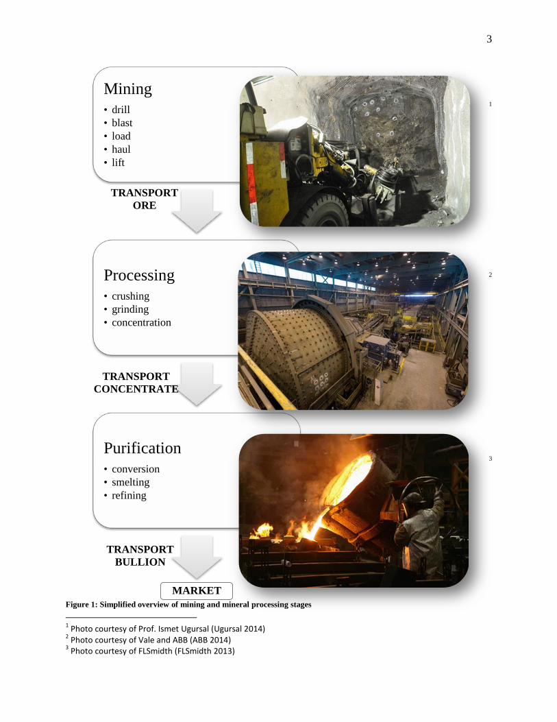
(Hartman, Mutmansky 2002). Figure 1 shows a simplified overview of the mining stages used to

produce bullion from ore. These are the stages in what we refer to as a ‘Mine toBullion’ audit

methodology.

3

Mining • drill • blast • load • haul • lift

Processing • crushing • grinding • concentration

Purification • conversion • smelting • refining

1

2

3

Figure 1: Simplified overview of mining and mineral processing stages 1 Photo courtesy of Prof. Ismet Ugursal (Ugursal 2014) 2 Photo courtesy of Vale and ABB (ABB 2014) 3 Photo courtesy of FLSmidth (FLSmidth 2013)

TRANSPORT ORE

TRANSPORT BULLION

TRANSPORT CONCENTRATE

MARKET

4

In some cases the products of mineral production are basic necessities for human existence

where population growth is a significant factor in the demand for the sector’s commodities.

However advances in technology and a desire for economic growth from developed and

developing countries drive demand further. The basic economic equilibrium between supply and

demand indicates that increases in demand will lead to a higher commodity prices if there is no

corresponding change in supply (Frank, Bernanke et al. 2012b). Eventually, as ore bodies are

mined out, mineral supply will decline and lead to further price increases. Conversely, lower

operating costs associated with technological development may enable mining of ore bodies that

were once considered uneconomical. Energy management is an area for technological

development that may lead to lower operating costs, and thus allowing society to maintain or

enhance current standards of living while keeping costs affordable.

1.2 Energy use in mining

Mining is an energy intensive industry with substantial environmental impacts (Mudd 2010).

Different energy sources are used during the various stages within the mining and mineral

processing stages as illustrated in Figure 2 which was produced with actual data from Vale’s

Sudbury operations.

Six types of energy are used for these specific mining and processing stages; electricity is mainly

used to for support activities in mines (ventilation, hoisting, pumping, compressed air, drilling)

and for breaking ore in the processing stages, natural gas and propane are used as heating fuels

(comfort or process heat), whereas gasoline and diesel are employed for transportation purposes,

and coke is used as a reducing agent.

5

Figure 2: Sankey diagram illustrating the energy consumption of the mining and processing stages

6

The amount of energy used in the various stages of the process is influenced by different support

variables as illustrated in Table 1. In addition to these, which are specific to the orebody, mine

location can also affect energy use; more energy is used to heat buildings and mine ventilation

air in colder climates whereas cooling is required in hot areas.

Table 1: Support variables and their effect on the mining and mineral processing stages

Stage Effect on energy consumption

Mining

drill and blast harder ore needs more energy

load and haul lower grade ore requires more material to be transported

lift deeper ore bodies need more energy to bring ore to surface

Processing

crushing and grinding smaller minerals require more comminution, thus more energy to liberate,

harder ores require more energy to break

lower grade ores requires more material to be processed and transported per unit of mineral

concentration lower grade ores requires more material to be processed and transported per unit of mineral

Purification

conversion, smelting, refining mineralogy affects the amount of energy required to ‘melt’ the material

In 2010, the proportion of total costs spent on energy averaged 15% and 19% for Canadian metal

and non-metal mines respectively. Although energy corresponded to the smallest share of total

7

costs, it was the only category that has shown an increasing trend since 1961 (Natural Resources

Canada 2012a, Statistics Canada 2013). It can be postulated that the proportion of total

expenditure associated with energy in the mining sector is increasing due to a combination of

factors such as rising energy rates or mines consuming more energy as they mine from deeper

levels or process lower grade ores. Figure 3 illustrates the Canadian industrial energy prices from

1990 to 2012 in constant dollars (base year 2002). It shows that with the exception of natural gas,

energy prices have stayed the same or increased. The most prominent increases are for fuel oils

on which the sector depends.

Figure 3: Canadian energy prices 1990-2012 - constant dollars (Natural Resources Canada ca. 2014, Statistics Canada 2015)4

4 Industrial energy price data published by Natural Resources Canada (ca. 2014) were provided using current dollar amounts however when comparing economic figures over time it is more appropriate to utilize constant dollars in order to eliminate the effect of inflation. Using consumer price index (CPI) for energy (Statistics Canada 2015), the current values were converted to constant values with a base year corresponding to 2002.

0

20

40

60

80

100

1990 1995 2000 2005 2010

Cons

tant

Cos

t -Ba

se Ye

ar: 2

002

(CAD

)

Natural Gas (cents/m3) Light Fuel Oil (cents/litre)

Heavy Fuel Oil (cents/litre) Electricity (1,000 kW/400,000 kWh) (cents/kWh)

Electricity (5,000 kW/3,060,000 kWh) (cents/kWh)

8

Figure 4 shows the Canadian mining industry energy consumption for the same period. The trend

is clearly one of increase for the mining sector as a whole but this is mainly due to the petroleum

sub-sector.

Figure 4: Canadian mining industry energy consumption 1990-2012 (Natural Resources Canada ca. 2014)

0

200

400

600

800

1,000

1,200

1990 1992 1994 1996 1998 2000 2002 2004 2006 2008 2010 2012

Ener

gy C

onsu

mpt

ion

(PJ)

Upstream Mining (petroleum) Copper, Nickel, Lead and Zinc Mines Iron MinesGold and Silver Mines Other Metal Mines Salt MinesPotash Mines Other Non-Metal Mines Total mining industry

9

Figure 5: Canadian metal and non-metal mining industry energy consumption 1990-2012 (Natural Resources Canada ca. 2014)

Examination of the energy use from the Canadian metal and non-metal sub-sectors in Figure 5

reveals that energy use from 2000 to 2007 was relatively stable. In 2008 energy use increased,

mostly influenced by the iron industry which may have increased production output as a

response to high iron prices but in 2009 energy use returned to previous levels. An appraisal of

the current energy situation in the mining sector is limited due to the most recent data published

corresponding to 2012, but the trend from 2010 to 2012 suggests that energy use is on the rise

due to increasing consumption from copper, nickel, lead and zinc mines, as well as potash mines.

Figure 6 presents a breakdown of the energy use per tonne of ore milled by energy type for the

Canadian copper, nickel, lead, and zinc mines from 1990 to 2012. The data illustrates that from

2007 to 2012 more energy was consumed per tonne of ore milled.

0

20

40

60

80

100

120

140

160

1990 1992 1994 1996 1998 2000 2002 2004 2006 2008 2010 2012

Ener

gy C

onsu

mpt

ion

(PJ)

Copper, Nickel, Lead and Zinc Mines Gold and Silver Mines Other Metal MinesIron Mines Salt Mines Potash MinesOther Non-Metal Mines

10

Figure 6: Canadian copper, nickel, lead, and zinc mines energy intensity 1990-2012 (Natural Resources Canada nd)

It can be observed from Figure 6 that over the period natural gas and electricity intensity have

reduced slightly, by 11% and 8% respectively, whereas diesel intensity increased by 74% from

1990 to 2012. Since diesel is principally used to transport ore, this shift may indicate that active

mining is occurring at locations farther away from the shaft. Conversely, it is expected that the

trend in electricity intensity would follow that of diesel since ventilation systems consuming

electricity are used to dilute the emissions produced from diesel use, thus an increase in diesel

consumption should result in an increase in electricity consumption. This discrepancy may

reflect the positive effect electricity conservation measures such as ventilation on demand, or

more efficient motors. However, a comprehensive analysis of the energy intensity is not possible

without specific information that would indicate structural shifts and support variables that affect

energy use such as the mine depth, ore grade, hauling distances, and climate.

0

10

20

30

40

50

60

70

80

90

1990 1992 1994 1996 1998 2000 2002 2004 2006 2008 2010 2012

Ener

gy in

tens

ity (k

Wh/

tonn

e or

e m

illed

)

Electricity Natural Gas Diesel Fuel Oil, Light Fuel Oil and Kerosene Heavy Fuel Oil LPG and Gas Plant NGL Coal

11

Regardless of the trends and variability of energy use and intensity in the sector, it is clear that

despite the prominence of energy issues and energy conservation initiatives there has been no

step change improvement with respect to energy consumption in the mining sector in these

census periods.

In a macro-economic context for the Canadian mining industry, at least, it appears that the

mining sector may be on the verge of a ‘perfect storm’ of increasing energy input prices,

increasing depths of production, and lower ore grades, and this is what has motivated the

research conducted and reported in this thesis. In other sectors of industry, the mantra of

prioritization of effort with respect to energy is: use less energy (waste less); use what energy

one has to more efficiently (increase efficiency); and then utilize energy sources that have much

lower marginal costs (renewable).

12

1.3 Objectives

In this work, the opportunities that present in the first two areas are focused upon elimination of

wasted energy and implementation of more efficient technologies, both brought about by

improved energy management systems. The main objective for this research was to identify

whether a robust energy management methodology for mineral production processes (from mine

to bullion) could be developed, and to exemplify parts of such a methodology to highlight

economic benefit and further potential.

It is presumed that critical review and possible modification of existing methodology to:

i) manage energy,

ii) identify priority areas for improvement and,

iii) assess viability of projects

are necessary in order to render them applicable to any mineral operation; whether a mine, a

processing facility or an integrated mining and process operation.

Although a ‘mine to bullion’ energy audit framework was an ambitious undertaking, the scope of

this research aimed to set out such a framework upon which further work could build upon, as in

a continuous improvement process.

There may be obstacles for the mining industry to overcome to realize the full benefits of energy

management, thus this research will examine the evolution of energy management practices

adopted by the Canadian mining industry in the past as well as the barriers and drivers that were

associated with progress in this sector.

13

Although the North American Industry Classification System’s definition of mining comprises

metals, non-metals as well as fuels (Statistics Canada 2012), this thesis focuses on the metals

sub-sector. The Canadian mining sector is specifically examined because it is a major contributor

on a national as well as a global basis. In 2013, the mining sector provided 3.4% of Canada’s

Gross Domestic Product (GDP), and has contributed as much as 4.5% of GDP within the last 20

years. On a global scale, Canada is among the top 5 countries for production of 11 minerals and

metals, which include among others: potash, uranium, cobalt, tungsten, nickel and diamonds

(The Mining Association of Canada ca. 2015).

1.4 Thesis outline

A critical review of energy management initiatives implemented in the mining industry will be

presented in Chapter 2 to determine what progress has been achieved during the past 40 years.

Sub-sections examining the barriers and drivers to energy management practices are also

included in this chapter so that consideration is given to motivation and obstacles during the

development of the energy management framework for the mining sector.

Innovation in any area requires access to reliable data, thus a critical review of mining energy-

related data will be presented in Chapter 3. Energy savings from conservation measures can be

masked as mines extract ore from deeper levels and thus consume more energy. A case study,

presented in Section 3.1.6 develops this key understanding and identifies the need for reporting

additional data. Chapter 3 also develops a benchmarking metric for the framework,

encompassing the most significant variables that affect energy use in a mine including: mine

depth, production, and climate. Mines normalizing against these variables may be able to

legitimately compare own performance through time, or compare performance to others with the

14

use of internal and external benchmarking within the framework. The use of this metric may also

be extended to forecasting energy consumption of a mining development either at the design or

operational phase.

Chapters 2 and 3 comprise sections that have been published in the Journal of Cleaner

Production Special Volume – The sustainability agenda of the minerals and energy supply and

demand network: an integrative analysis of ecological, ethical, economic, and technological

dimensions (Levesque, Millar et al. 2014).

The first step in energy management corresponds to understanding how and when energy is

consumed. As there are different methods for conducting energy audits, there is a need to assess

the applicability of these existing methodologies to the mining sector. In Chapter 4, a review of

existing energy audit methodologies is included to support the development of a framework for

energy management tailored for the mining sector. The work reported in Chapters 2 to 4 formed

the basis for the formulation of the key research questions presented in Chapter 5 that were at the

heart of the investigations reported in the following chapters.

In Chapter 6 best practice examples for energy management will be critically reviewed; some are

specific to the mining sector whereas others are of a general nature. Examples of implemented

energy management initiatives in the mining industry were assembled in a database providing i)

a standardized reporting framework and ii) opportunity for dissemination of best practice energy

conservation measures for the mining sector. The work reported in this chapter was previously

published and presented at the 2013 World Mining Congress (Levesque, Millar 2013, Levesque,

Millar et al. 2014).

15

A review of an energy audit conducted for an underground mine ensues in Chapter 7.

Recommendations for an improved audit methodology for mines are provided in this chapter.

Having gathered energy data via an energy audit from an underground mine, the next step should

comprise of an analysis stage whereby potential energy conservation measures are identified.

Ventilation corresponds to the largest energy consuming end-use in an underground mine thus

Chapter 8 comprises a ventilation study to demonstrate potential energy savings within this sub-

system in an underground mine. Techno-economic assessments of hypothetical scenarios were

made to determine the viability of energy conservation initiatives and to determine how savings

could be enhanced. This chapter also provides recommendations for an improved methodology

for conducting ventilation surveys to determine duct friction factors, an important factor used in

mine design and for decision making.

Conducting energy audits can be challenging in a mining environment due to the large number of

equipment items, especially in mines lacking sub-meters for measurement of energy

consumption from various end-uses. This lack of information may hinder identification and

approval of energy conservation projects by decision makers. In chapter 9 a novel disaggregation

analysis was developed to estimate the electricity consumption by end-uses in an underground

mine from the data obtained from the mine’s main electricity meter. This draws upon expert

knowledge of defining characteristics of the mine’s energy use. A case study is presented in

Chapter 9 to illustrate the use of this disaggregation methodology to estimate the electricity

consumed by a hoist in an underground mine. Further development and adoption of this concept

could lead to a simpler and cheaper energy auditing system, thereby reducing the number of sub-

meters and associated communication infrastructure and data storage requirements.

16

Subsequently, a review of a detailed energy audit conducted at a milling facility is presented in

Chapter 10. This work highlights the benefits of an energy balance approach to reconcile the

bottom-up audit data to establish true understanding of consumption drivers and true

conservation of energy and demand. The work presented in Chapter 10 was included in a

previous publication (Levesque, Millar 2015b).

Chapter 11 is included for completeness of the ‘Mine to Bullion’ energy audit and comprises a

brief summary of an energy audit conducted for a pyrometallurgical process. The work included

in this chapter was previously published as part of a Master’s thesis (Levesque 2011).

The findings from the preceding chapters will be synthesized in an extended discussion

presented in Chapter 12. Strategies for improved energy audits, enhanced communication, and

better data interpretation are discussed within the context of an improved energy management

methodology for the mining sector.

The final chapter will present the conclusions of the work and the contributions to the discipline

of mine energy management that arose during the execution of this research. The thesis closes by

outlining the key actions to further develop this work and to realize even more economic benefit

for the minerals industry.

17

2 A critical review of energy management progress in the mining industry

2.1 Energy management timeline

Over several decades, milestone publications, regulations, committees and guidelines pertaining

to energy management and conservation have emerged. These, among others, are illustrated in

Figure 7 along with the fluctuation in crude oil prices (BP 2012) .

It can be seen from Figure 7 that the increase in crude oil prices in the 1970’s coincided with the

first identified journal publication pertaining to energy management in the mining sector in 1973.

In 1975, the Canadian Industry Program for Energy and Conservation (CIPEC) was formed

(Natural Resources Canada 2011a) and the Battelle Columbus Laboratory, sponsored by the

United States Bureau of Mines, published the following studies, “Energy Use Patterns in

Metallurgical and Nonmetallic Mineral Processing” (Battelle Columbus Laboratories 1975) and

“Evaluation of the Theoretical Potential for Energy conservation in Seven Basic Industries”

(Hall, Hanna et al. 1975). Subsequently, as crude oil prices decreased, the focus on energy

continued with publications describing the energy conservation efforts of various mining

companies (Manian 1974, Tittman 1977, Armstrong 1978, James 1978, Doyle 1979, Cullain

1979, Harris, Armstrong 1979). These papers are not included in Figure 7 because they are not

considered to be ‘milestones’ since they were published after Lambert (1973) but they will be

discussed in the next section.

From 1985 to 1989 the Department of Energy, Mines and Resources Canada published a series

of energy management manuals to assist organizations in identifying energy conservation

measures in areas including: lighting, process furnaces and dryers, energy accounting and

automatic controls (Energy Mines and Resources Canada various).

18

Figure 7: Chronology of crude oil prices and milestones relating to energy management in the mining industry. Source: Figure designed by the authors based on references related to the publications and initiatives cited in text

1973 - Lambert (first identified journal publication)first oil shock1975 - CIPEC, Batelle Columbus Laboratories Report

second oil shock

1989 - Energy Efficient Technologies in the Mining and Metals Industries Seminar

1991- ICME1992 - Energy Efficiency Act1993 - Energy Efficiency R&D Opportunities in the Mining and Metallurgy Sector, CIEEDAC1994 - MAC Whitehorse Mining Initiative, OMA energy task force1995 - Energy Efficiency Regulations 1996 - Kyoto Protocol adopted by Canada1997 - GRI founded

2000 - UN Global Compact, GRI G1, OMA energy committee2001 - ICMM formed from ICME2002 - GRI guidelines G2

2004 - Energy Efficiency Regulations amended, MAC TSM2005 -Canadian mining benchmarking studies UG and Open pit mines2006 - GRI G3, EEO program2007 - US DOE Mining Energy Bandwidth Study

2010 - NIERP 2011 - GRI G3.1, ISO 50001, Canada withdraws from Kyoto Protocol

1985 to 1989 - Energy, Mines and Resources Canada - Energy Management Series for Industry, Commerce and Institutions

1970

1975

1980

1985

1990

1995

2000

2005

2010

0 50 100 150

Crude Oil Prices ($2011)

19

In 1989, a seminar entitled “Energy Efficient Technologies in the Mining and Metals Industry”

was held, highlighting industry as well as research and development projects which were co-

funded by the Ontario Provincial Government through the Ministry of Energy (University of

Toronto, Ontario et al. 1989). The papers published in the proceedings included inter alia: Heat

recovery from mine waste water at LAC Minerals, Development of the Kiruna electric truck at

Kidd Mine and Mine energy usage – a mine superintendent’s perspective from Inco Limited

(now Vale).

Heat recovery from mine waste water at LAC Minerals described an energy conservation project

that was implemented at the Macassa Mine to recover waste heat from mine drainage water and

air compressors. The recovered heat was used to heat the mine ventilation air, thus displacing

natural gas to prevent freezing in the shaft. An estimated 80% reduction in natural gas cost

resulted from the first four months of use of the waste heat recovery system. The study also

compared the budget and actual amounts for the various equipment categories. It was shown that

the actual spending on the heat recovery system was 13% greater than anticipated due to

increased labor costs and additional piping requirements. Conversely, the monitoring and control

systems cost 105% more than estimated due to design considerations implemented after

completion of the budget and a lack of expertise with application of this equipment in the mining

sector. Thus this highlights the importance of the planning stage of an energy conservation

project as well as the value of experience and knowledge within the mining industry.

The paper titled ‘Development of the Kiruna electric truck at Kidd Creek Mine, Falconbridge

Ltd.’ presented a summary of a feasibility study conducted to investigate the financial viability

of using electric trucks as a hauling system for a mine expansion project. Energy savings of 39%

were estimated from use of electric haul trucks as opposed to diesel vehicles. These estimated

20

energy savings were due to the lower power requirements from the electric trucks and thus

reducing the ventilation requirements. Although there were no actual results available to confirm

these savings, it is suspected that the financial viability of this project electric was favorable

since Kiruna trucks were still used at Kidd Creek Mine in 1995 (Paraszczak, Fytas et al. 2014)

The Mine energy usage – a mine superintendent’s perspective paper presented the relative

amounts of electricity used by the different mining and mineral processing stages of Inco’s

Sudbury operations (now Vale), which compared well with the values from Figure 2. A

breakdown of the typical costs incurred by South Mine was also included, which showed that

energy (electricity, natural gas and fuel) accounted for only 7% of total expenditures for this

mine. Thus energy conservation was not a priority at this site but electric scooptrams were

introduced due to the additional benefits from their use. It was stated that “The main reason for

the move to electrics, aside from the environmental benefits, were to improve productivity and

reduce maintenance costs. These criteria are essential to justify equipment change.” It was

shown that the electric vehicles consumed less energy per ton, had higher production measured

in tons per hour, and lower maintenance costs, than their diesel counterparts. It was also stated

that energy costs are largely determined by the mine design thus “the most effective way to affect

efficient energy utilization in a Mine is right at the design stage.” Another finding in this

publication was that energy and maintenance costs were lower, and that production was higher

for larger equipment. It was suggested by the superintendent that larger electrically powered

equipment may be used as an energy management initiative. However, the higher capital and

development costs arising from the use of larger equipment should be balanced against the

benefits to determine the economic viability of this measure.

21

During the 1990’s the attention on energy efficiency progressed with the adoption of the Energy

Efficiency Act in 1992 which developed into the Energy Efficiency Regulations in 1995

(amended in 2004). The goal of these regulations was to provide minimum energy performance

levels for a range of energy-consuming products purchased in Canada, as well as to dictate the

inclusion of labels stating the estimated annual energy consumption of some products on the

market (Canadian Institute for Energy Training 2006). In 1993, Natural Resources Canada

published a study entitled “Energy Efficiency R&D Opportunities in the Mining and Metallurgy

Sector” (Sirois 1993), and the Canadian Industrial Energy End-use Data and Analysis Centre was

created. The formation of the Ontario Mining Association’s (OMA) energy task force in 1994

developed into a standing committee in 2000 (Brownlee 2012). The Mining Association of

Canada (MAC) launched the Whitehorse Mining Initiative in 1994 which ultimately evolved into

the association’s Towards Sustainable Mining initiative in 2004 (Fitzpatrick, Fonseca et al.

2011).

These efforts aimed towards energy efficiency emerged during periods of low oil prices between

1985 and 2000. Thus it is suspected that the guidance was developed as a proactive approach in

anticipation of rising energy prices so that industry would be better positioned to face increased

operating costs.

Since 2000 there has been a surge in sustainability initiatives with the development of reporting

guidelines by several organizations such as the UN Global Compact, the Global Reporting

Initiative (GRI) and the International Council on Mining and Metals (ICMM), with the aim of

increasing corporate transparency with respect to economic, environmental and social impacts.

Natural Resources Canada published two studies in 2005 titled “Benchmarking the energy

consumption of Canadian Underground Bulk Mines” and “Benchmarking the energy

22

consumption of Canadian Open-Pit Mines” (Canadian Industry Program for Energy

Conservation 2005b, Canadian Industry Program for Energy Conservation 2005a).

In 2006, the Australian government launched its Energy Efficiency Opportunities Program that

requires users annually consuming more than 0.5 PJ (~278 GWh) of energy to conduct an audit

to identify measures to improve energy efficiency (Australian Government Department of

Resources, Energy and Tourism 2011b). Additionally, the identified initiatives had to be reported

and were segregated by industry type. The energy conservation measures for the mining industry

are compiled in a database which can be accessed via the internet (Australian Government

Department of Resources, Energy and Tourism 2011a). In 2007 the US Department of Energy

released a publication titled “Mining industry Energy Bandwidth Study” which estimated

potential energy savings of 54% for the U.S mining industry (U.S. Department of Energy 2007).

The Northern Industrial Electricity Rate Program (NIERP), created in 2010 and administered by

the Ontario Government, promotes energy management by offering rebates on electricity rates to

large industrial users in northern Ontario who have prepared an energy management plan

(Ministry of Northern Development, Mines and Forestry 2010).

Clearly the topic of energy management has accrued some importance in the past 4 decades, but

what has actually been achieved? Have the suggestions from the 1970’s been adopted as best

practice? Have any innovative solutions been developed?

2.2 1970’s initiatives

As energy prices were increasing, the industry recognized that energy management was

necessary. A review of publications has revealed that the earliest paper found so far pertaining to

energy management and conservation in the mining sector dates back to 1973.

23

Lambert (1973) promoted energy conservation through utilization of waste heat from electric

motors, compressors and fossil-fueled electricity generators. He stated that “The fact that there is

no energy crisis today does not mean that there will not be such a situation in the years ahead. In

any case, an abundance of energy is still no excuse for not making the best possible use of all

energy forms.”

Manian (1974) presented a paper focusing on energy reductions from process and space heating

in a mine and ore processing mill with the following measures:

• Substitution of air stirring with mechanical means

• Substitution of air with oxidizing compounds

• Covering process tanks to reduce heat losses

• Implementation of heat recovery measures

• Insulating tanks

• Improved building insulation

• Use of a heat pump.

In Tittman (1977) the energy conservation efforts at Erie Mining Co. were published. The

company established a conservation program in 1973 with a group to assess energy use and an

employee training program through which the following measures were identified for energy

management:

• Preventative maintenance on power plant steam traps

• Reducing fuel spills

• Fixing compressed air leaks

24

• Correcting everyday energy waste, such as eliminating vehicle idling

• Education program for employees concerning vehicle idling and turning off lights

• Installation of oxygen analyzers on boilers to control excess air and optimize fuel

combustion

• Shutting down heating plant when not required

• Installation of more efficient lighting.

Financial savings generated by energy management result from lowering energy consumption

and from reducing the peak demand in any given billing period (Armstrong 1978). Armstrong’s

paper focused on demand side energy management efforts in the milling stage of a mining

operation by utilizing a rod mill as an example, which showed that the reduction of peak demand

and energy consumption both result in lower energy costs. Armstrong also illustrated that

operation of the rod mill at rated production capacity resulted in lower specific energy

consumption in kWh/ton, and reduced unit energy cost.

James (1978) highlighted the following benefits associated with energy efficiency: i) reduced

energy consumption will lead to reduced costs, resulting in increased profits and enhanced

competitiveness, ii) lower energy demand will extend life of current energy sources and iii)

lower energy bills will liberate funds which would have been allocated for energy supply.

Furthermore, James identified three levels of opportunities for improvement. The first level

corresponded to ‘housekeeping’ measures which could typically yield improvements of 10-15%

with little or no cost for modifications to operating procedures and equipment maintenance. The

second level of opportunities also led to 10-15% savings, but with time or financial investment

requirements. The final level involved ‘total plant energy flow optimization and equipment and

25

process design’ which could result in improvements beyond the 20-30% savings achieved with

the first two levels. James’ analysis of Canadian non-metal mines showed that energy

consumption as well as unit energy costs in this sector were increasing in the early 1970’s. He

also examined the share of fuel and electricity costs relative to total production costs and found

that this metric was also increasing, as did materials and supplies whereas the percentage

associated with production wages was decreasing. James concluded “Energy savings mean

dollar savings. In the late 1970’s and beyond, no company or industry can afford to treat energy

as a low priority” (p.103).

According to Wenzl (1978), the Inco Metals Company launched an Electric Power Management

Program in 1972 that had the goal of controlling peak power and was successful at improving the

power load factor to over 90% in 1976 from 83% in 1973. Load factor corresponds to the ratio of

the average demand to the maximum demand for a period (Doty, Turner 2009) and lower values

may result in higher billing rates depending on the rate structure of the utility; it can be favorable

to redistribute the load in a billing period to increase the load factor. The program included

monitoring power consumption to establish a load profile at each plant and mine as well as the

installation of power consumption monitors to forecast the demand and assist operators to

manage the total power consumption. Subsequently, the program was expanded with the

formation of committees at each site which identified potential savings by reducing compressed

air and ventilation during periods of low underground activity. The program resulted in

electricity demand reductions of 1,400 MW (1.4 GW) and over 280,000 m3 (10,000 mcf) of

natural gas savings per year for one mine (Wenzl 1978). However, such electricity savings are

questionable, as this represents roughly 10% of current electricity demand in Ontario, but

Wenzl’s electricity savings may actually correspond to 1,400 MWh per year.

26

At Falconbridge Nickel Mines Limited, energy management efforts in 1979 consisted of:

identifying major energy consumers, installation of meters and controls, dedication to lowering

unit energy consumption, promoting conservation through revised accounting practices and

development of an energy management policy at Westfrob Mine in British Columbia (Doyle

1979). The operation realized the importance of load and demand profiles to understand when

and how energy was utilized to identify measures for reducing consumption and/or demand,

which could also result in cost savings. Subsequently, an energy audit was conducted at the

Sudbury operations where energy management initiatives included waste heat recovery from

compressors and mine air, and shutting down equipment such as compressors, pumps, fans and

heaters when not required, which has resulted in annual savings of 0.9 million dollars, or about

2.7 million dollars ($2013)5

A compressed air study was conducted at Inco Metals Company’s Levack Mine Complex and

according to Cullain (1979) it was determined that an excess of 28% air was generated compared

to theoretical requirements and that the excess air consumption occurred during non-production

periods. Subsequently, corrective actions were taken which resulted in a 15% compressed air

consumption reduction and electrical power savings of $80,000 per annum, or about $245,000

($2013), which corresponded to roughly 5% of total mine electricity consumption (Cullain

1979). The measures comprised of fixing leaks, reducing compressor usage during off-shift and

weekends and increasing employee awareness with respect to compressed air waste and efficient

use (Cullain 1979).

. This corresponds to roughly 6% of annual energy expenses, with

minimal capital expenditures (Doyle 1979).

5 Bank of Canada, 2013. Dollar values from the 1970’s were indexed to $2013 but values from 2007-2012 were not adjusted since the rate of inflation during that period was quite low.

27

Harris and Armstrong (1979) published a paper outlining the electrical energy management

efforts at Inco Metals Company’s Shebandowan Mine, which identified that substantial savings

were achieved by “finding and fixing energy leaks”, as well as improving maintenance and

operating practices. It was stated that “One of the most difficult, but lucrative, ways to achieve

conservation of energy is to identify waste energy. A complete energy profile that accurately

describes the individual and total energy input for productive and non-productive functions, for

production and down-time periods, for peak and average activity levels, and for principle energy

utilization equipment is required. Waste energy during production periods is usually limited to

machinery that has high idling energy requirements. Finding waste which is not obvious or

occurs in small increments requires a systematic and critical review of every energy

connection.” The paper showed that reducing skip hoist speed, controlling peak load, shutting

down equipment during low production periods and the installation of outdoor lighting controls

are measures contributed to energy peak and consumption savings of 3% of annual electricity

costs, totaling $25,000 per annum in 1977, or roughly $76,000 ($2013) (Harris, Armstrong

1979). Although it was not specified how the reduction in skip hoist speed from 13.72 to 9.14

m/s achieved savings, it can be speculated that they arose due to: i) reduced acceleration rate or

period, ii) reduced braking power or period, and iii) reduced air drag on the ore skips. When the

hoist is travelling at a constant speed, the force required to keep the unit moving corresponds to

the drag, which according to Streeter and Wylie (1983) is characterized by:

𝑭𝑫 = 𝑪𝑫𝑨𝝆𝑼𝟐

𝟐 (1)

where 𝐶𝐷 is the drag coefficient, 𝐴 is the area, 𝜌 is the density and 𝑈 is velocity. According to

(1), the only factor which affects the drag in this instance is the velocity since all other values are

28

constant. Therefore it is estimated that a reduction in skip hoist speed from 13.72 to 9.14 m/s

would reduce the energy consumption by a factor of at least 2.25. Lowering the acceleration of

the skips from or to rest may have also reduced the peak power demand of a hoist cycle. This

measure would result in a longer hoisting cycle therefore, prior to implementation an assessment

should be conducted to investigate the effect on production.

This section provided examples of energy management efforts of the 1970’s at various mines

that resulted in financial savings ranging from 3 to 6%, through reducing peak demand, lowering

demand charges and through energy consumption savings by eliminating wasted energy. These

savings were achieved because operations management understood where and how energy was

utilized through energy audits and metered consumption. Although some of the mine sites from

these examples are no longer in operation, the companies who owned them still exist and are

operating other sites, however, there is conflicting evidence that the energy management efforts

from this era are still being practised, sustained or have evolved.

2.3 Recent initiatives

40 years have passed since the publication of the earliest article reviewed with respect to energy

management in the mining industry, but what progress has the industry made?

The first observation is that companies have switched from publishing energy conservation

efforts in journals to promoting them in corporate sustainability reports and industry newsletters

and publications, which are not peer reviewed. Second, most of the papers relating to energy

management in the mining industry that have been published in academic journals or conference

proceedings pertain to research and development projects as opposed to implemented measures.

29

A survey of recent energy conservation efforts in the Canadian mining industry dating back to

2007 has revealed several initiatives. These initiatives were compiled from corporate

sustainability reports (DeBeers, Xstrata, Teck and Diavik), Sudbury Mining Solutions Journal, a

study conducted for the Ontario Mining Association, Heads Up CIPEC newsletter, a media

release from Rio Tinto, corporate websites (Diavik and Goldcorp) and proceedings from the

International Conference on Renewable Energies and Power Quality.

Mines located in northern Canada have implemented measures to recover heat from diesel

generators deployed and operated for the production of electricity and are utilizing this heat to

warm buildings. DeBeers’s Snap Lake mine has estimated that annual diesel fuel consumption

has been reduced by 800,000 to 1 million litres, or approximately 3% of total consumption by

increasing the size of their heat exchangers (DeBeers Canada ca. 2011). At Diavik Diamond

Mine, the diesel power plant energy utilization is cited as over 80% (Diavik Diamond Mine n.d.)

which is a substantial improvement compared to the typical diesel generator efficiency of about

33-40% when electricity is produced alone (Deshpande 1966).

At Xstrata Zinc’s Brunswick Mine the heat recovered from the concentrate dryers is used to

warm the flotation slurry and in 2007, resulted in annual savings of $850,000 corresponding to

16% in avoided steam consumption, which was previously required to heat the slurry (Xstrata ca.

2007). Subsequently, the company has implemented measures, such as recirculating water in the

thickeners and heat recovery from cooling compressors to double the amount of recovered waste

heat, from 30 GJ/h (8.3 MW) in 2007 (Xstrata ca. 2007) to 60 GJ/h (16.6 MW) (Natural

Resources Canada 2012b).

30

When considering waste heat recovery, it is important to consider the grade of the available heat

to match the source with an area in the process that can maximize the efficient use of this energy.

This can be achieved using Pinch Analysis, which is a widely used Process Integration method.

According to Natural Resources Canada (2003), “It provides tools that allow us to investigate the

energy flows within a process, and to identify the most economical ways of maximizing heat

recovery and of minimizing the demand for external utilities.” In essence, these are techniques

that match the grade (temperature) of waste heat to parts of a process that require heat of roughly

the same grade. The ‘pinch’ refers to the minimum difference between the temperatures of the

source (waste) heat and the application. Methodology and additional applications of Pinch

Analysis can be found in Linnhoff and Flower (1978), Flower and Linnhoff (1978), Linnhoff and

Hindmarsh (1983) as well as Linnhoff (1993).

A second category of initiatives consists of common sense measures to reduce waste energy.

Both Teck and Rio Tinto have reported shutting down equipment when it is not required as a

means of reducing energy consumption (Teck ca. 2007, Rio Tinto ca. 2010), which at Teck’s

Hemlo operations included ventilation.

Diesel fuel reductions for material hauling equipment during idling periods can also lead to

substantial savings from anti-idling policies and installation of new heating equipment. At

Goldcorp’s Porcupine Gold Mine, heaters were installed to keep the engine and operator cab

warm during the winter when vehicles were stationary (Tollinsky 2011). Such an initiative has

resulted in estimated annual savings of about $300,000 or over 3% of total diesel cost, with a

payback period corresponding to less than one year including the cost of new equipment.

31

Another initiative which is gaining attention is Ventilation On Demand (VOD) where the supply

of fresh air delivered underground is matched with the demand, which reduces ventilation system

use. The simplest implementation of this is by turning auxiliary fans off when they are not

required. Another method is the modulation of auxiliary fans through high-half-off settings,

requiring relatively inexpensive equipment (Allen 2012) and the most complex and most

expensive method is the continuous modulation of auxiliary fans through the use of Variable

Frequency Drives (VFD). For example, Xstrata Nickel reported annual energy savings of 10% at

its Nickel Rim South Mine (Xstrata Nickel ca. 2010), and Xstrata Zinc’s annual savings at

Brunswick mine corresponded to $700,000 (Natural Resources Canada 2012b). At Vale’s

Creighton Mine the potential energy savings were reported at $20,000 per fan per annum by

reducing the fan speed by 10%, corresponding to a 27% energy savings (Vale ca. 2010).

Comparison and analysis of these initiatives was not possible due to the lack of standardized

reporting and incomplete information. For example, total energy use at Brunswick mine was not

reported. Therefore, it was not possible to assess the significance of the financial savings relative

to the total energy cost. Furthermore, VOD may also lead to reduction in heat requirements, but

it was not specified whether the Brunswick mine savings included these or corresponded only to

decreased electricity consumption.

Another energy consumption reduction measure in this category consists of fixing compressed

air leaks. At Xstrata’s Brunswick mine a small team is responsible for monitoring and repairing

such leaks (Natural Resources Canada 2012b), which can represent significant losses, if left

untreated. For example, in a study prepared for the Ontario Mining Association, da Cunha (2007)

conducted a compressed air leak study involving three mines; FNX (now KGHM International)

McCreedy West, CVRD Inco (now Vale) South Mine and Barrick’s Williams Mine. The study

32

indicated that most compressed air leaks in mines occur from the effects of blasting or by mobile

equipment striking pipes. The common locations of leaks include: couplings, cracked or

damaged hoses, tubes and fittings, open condensate traps, pipe disconnects, pipe joints, pressure

regulators, shut-off valves and thread sealants. The report concluded that fixing large compressed

air leaks at two of these mine sites resulted in approximate annual energy savings of $100,000.

Savings identified by da Cunha were less than 1% of the total electricity consumption from one

of the sites, but could represent approximately 50% of the compressed air produced. Although

these savings may not seem significant, the situation would be different for mines using more

compressed air, which may have been the case with Xstrata’s Brunswick mine.

The final initiatives can be grouped into the renewable energy source category, which includes

wind, solar and geothermal. These sources of energy are typically used in the minerals industry,

when economically feasible, to lower fossil fuel consumption, which in turn reduces greenhouse

gas emissions (McLellan, Corder et al. 2012).

Goldcorp’s Musselwhite Mine installed a SolarWall®ventilation air heater on the mechanical

shop building on the basis of a calculated annual energy savings of 413 MWh and a payback

period of less than 4 years (Goldcorp 2010), corresponding to roughly 1% of total propane

consumption. While the economics of this project were favorable for this location, an assessment

should be conducted prior to implementation to assess the available solar resource, as this type of

system may not be financially viable at every site. An assessment of the effectiveness of such an

initiative would also be beneficial for industry by comparing the estimated savings versus the

actual performance of this energy conservation measure, but no details on the operation of this

SolarWall® heater have been published.

33

Construction of a wind farm at Rio Tinto’s Diavik Mine is expected to reduce diesel

consumption at this mine site by 10%. The wind farm was commissioned on the 28th September

2012, and the $33 million investment is expected to be paid back within 5 years (Rio Tinto

2013). The Diavik Mine is located in a remote northern region where there is no available grid

electricity supply. As a result, this operation uses diesel generators on site to produce electricity,

now integrated with wind power. The diesel supply for the mine must be hauled and stored on

site, so any decline in diesel consumption while maintaining production produces a reduction in

the fuel transportation and storage requirements. As the mine moves towards a fully underground

operation, the electricity demand will increase due to underground water pumping, mobile fleet

as well as heating and ventilation requirements (Rio Tinto ca. 2010). When integrating

renewable energy sources with conventional fossil fuel generating systems (i.e. running both

systems together in parallel) in islanded configurations, the efficiency of the conventional system

will be lower when it is running at partial load (Trapani, Millar 2013). The success of such

projects needs to be monitored to establish whether there are benefits for the wider mining

industry in embracing wind-based, electricity generation technology. Also, Teck and Suncor

jointly funded a wind development project in Alberta comprising 55 turbines that will produce

88 MW of peak power, which is enough to supply 35,000 homes in the province (The Globe and

Mail 2010). The electricity generated from this wind farm will not be utilized directly by the

mining operations, but instead used to offset carbon emissions. Other examples of individual

mining operations producing energy from wind include MSPL Ltd in India, Barrick Gold’s

Veladero mine in Chile and El Toqui in Chile (Paraszczak, Fytas 2012).

Solar energy has also emerged as an option for electricity supply in the mining industry.

Specifically, Chevron Mining’s Questa site in New Mexico United States (Latitude:

34

36°42'15"N), has a 1MW concentrating photovoltaic installation built on the tailings area of the

mine, which has now ceased operations. Additional solar projects are planned to supply

electricity to Chilean copper mines (Paraszczak, Fytas 2012) and the use of solar thermal energy

in copper heap leaching processes has been investigated to increase solution temperatures, which

leads to improved metal recovery (Metkemeyer 2012, Piraino, Rimawi et al. 2012). Finally,

geothermal energy is being utilized to displace fuel oil for electricity generation at the Lihir Gold

Mine in Papua New Guinea and produces 75% of the operation’s power (Paraszczak, Fytas

2012).

In summary, the energy management and conservation efforts in the mining industry from the

1970’s focused on effective utilization of energy through waste heat recovery and eliminating

waste energy and some case studies provided energy consumption data, such as electrical

demand profiles and load duration curves. In comparison, recent initiatives report similar energy

conservation measures with the added implementation of renewable energy sources, but none

provided demand profiles or load duration curves. It appears that the rate of uptake from the

1970’s suggestions seems to be low, which could be due to the lower energy prices in the 1980’s

and 1990’s. However, with recent increases in oil price, the industry is now faced with a similar

situation as in the 1970’s, but the more recent fall in oil price may impede energy progress in the

mining industry.

2.4 Barriers to implementing best practice

According to Tittman (1977) at Erie Mining Co., the greatest barrier to implementing energy

conservation practice was “…to get 2800 employees to think in the same way about a subject and

to act in a uniform, organized manner to conserve when, in today’s atmosphere of plenty, they

35

can see little need to practice and perform in the most efficient manner.” This hurdle was

overcome with supervision, education and communication to ensure the success of the energy

management program. However, the situation at the moment is different – awareness of the finite

nature of fossil fuel supply and perception of climate change are greater than before. Therefore,

companies wishing to focus on energy efficiency may not need the same level of effort to

convince employees of the value of such a program.

A study prepared for the Ontario Mining Association’s Energy Committee in 2008, identified the

following barriers to the implementation of energy efficiency measures (Scott 2008):

• Projects require a short payback period – i.e. less than 6 years

• Mining personnel are focused on production as opposed to conservation

• Lack of performance incentives tied to energy conservation key performance indicators

for production personnel

• High financial risk of implementing major technological changes

• Competition for capital – minimum acceptable rate of return (ROI) corresponds to 8.5%

and

• Mines nearing their end of life do not have sufficient time to recuperate investments from

long-term projects.

While some of these barriers are valid, others can be perceived as unfounded; for example, with

such a focus on production without consideration of energy consumption, mining operations may

not realize their full, profit-maximizing potential. While production is important in generating

revenue, why are production costs not always considered? According to cost-benefit principles,

36

profit-maximizing firms should examine production costs, which include energy, to determine

the level of output that would generate the maximum profit (Frank, Bernanke et al. 2012a).

Production costs for the Canadian mining sector, excluding oil and gas extraction industries,

were examined for metal ore mines and non-metallic mineral mining and quarrying from 1961 to

2010, using data compiled from the Principal statistics of the mineral industries. The data is

available in CANSIM tables 152-0002 and 152-0005 (Statistics Canada 2013), which contain

statistics collected by Natural Resources Canada. The Annual Census of Mines (Statistics

Canada var.a) and the Canadian Minerals Yearbook (Natural Resources Canada 2011b) provide

the same data.

The first CANSIM table contained data from 1961 to 1997, and the second one focused on the

period from 1994 to 2008. The 4-year overlap of these tables allowed the data to be combined

and established a consistency between the sources, and clarified the varying nomenclature

adopted between them. Table 2 shows the corresponding categories between these sources.

Table 2: Corresponding nomenclature between CANSIM tables for mining sub-sectors

CANSIM table 152-0002 CANSIM table 152-0005

Total metal mines Metal ore mining

Total industrial minerals (aggregate of Total non-metallic mines, and Total pits and quarries)

Non-metallic mineral mining and quarrying

37

Statistics Canada discontinued publication of this data after 2008, and the statistical tables in

Natural Resources Canada’s Canadian Minerals Yearbook were not available online for years

beyond 2008. However, figures for 2006 to 2010 were obtained from Natural Resources Canada

(2012a) by special request.

The Principal statistics of the mineral industries tables contained annual costs for: i) fuel and

electricity, ii) materials and supplies, and iii) total salaries and wages. These were analyzed to

determine the relative cost of each component for metal ore mining, as well as non-metallic

mineral mining and quarrying. The results are presented in Figure 8 and Figure 9. The dashed

lines correspond to the data from CANSIM table 152-0002, the data points comprise data from

CANSIM table 152-0005 and the solid lines represent data from Natural Resources Canada.

Figure 8: Historical annual costs for Canadian Metal Ore Mining (Natural Resources Canada 2012a, Statistics Canada 2013)

0

10

20

30

40

50

60

70

1961 1965 1969 1973 1977 1981 1985 1989 1993 1997 2001 2005 2009

% o

f Tot

al C

osts

Materials and supplies (CANSIM 152-0002) Materials and supplies (CANSIM 152-0005)Materials and supplies (NRCan) Total salaries and wages (CANSIM 152-0002)Total salaries and wages (CANSIM 152-0005) Total salaries and wages (NRCan)Fuel and electricity (CANSIM 152-0002) Fuel and electricity (CANSIM 152-0005)Fuel and electricity (NRCan)

38

Figure 9: Historical annual costs for Canadian Non-Metallic Mineral Mining and Quarrying (Natural Resources Canada 2012a, Statistics Canada 2013)

For both mining sub-sectors, fuel and electricity costs were the lowest of all (Figure 8 and Figure

9), but this is not the case for all mining operations as energy costs vary depending on the

location and source. For example, Goldcorp’s Porcupine Gold Mine, located in Northern

Ontario, claimed that energy costs ranked second in terms of total operating costs (Goldcorp

2011).

The relatively low fraction that energy costs have historically represented of total production

costs may explain the low uptake of energy efficiency measures. This suggestion was echoed in

the paper titled “Mine energy usage – a mine superintendent’s perspective” published in the

Energy Efficient Technologies in the Mining and Metals Industries Seminar (University of

Toronto, Ontario et al. 1989), which indicated that energy costs corresponded to 7% of total

0

10

20

30

40

50

60

70

1961 1965 1969 1973 1977 1981 1985 1989 1993 1997 2001 2005 2009

% o

f Tot

al C

osts

Total salaries and wages (CANSIM 152-0002) Total salaries and wages (CANSIM 152-0005)Total salaries and wages (NRCan) Materials and supplies (CANSIM 152-0002)Materials and supplies (CANSIM 152-0005) Materials and supplies (NRCan)Fuel and electricity (CANSIM 152-0002) Fuel and electricity (CANSIM 152-0005)Fuel and electricity (NRCan)

39

expenditures, thus a substantial amount of energy savings would result in marginal overall

operating cost savings. Furthermore, it was reported that energy consumption is dictated by the

mine design, thus a minimum amount of energy is required for production. Although this was

perceived as a barrier to energy management, there is no excuse for wasting energy as expressed

in Lambert (1973).

The trends in Figure 8 and Figure 9 indicate structural shifts in production costs. In general the

share of costs for fuel and electricity has been growing. This trend was valid up to 2008, but in

2009, the share of energy costs relative to other operating costs decreased. This decline can be

associated with the economic downturn. For metal mines, spending on fuel and electricity, and

materials and supplies decreased in 2009 whereas costs for wages and salaries continued to

increase. For non-metal mines, all costs declined in 2009, but the reduced spending on wages and

salaries was less severe than the cutbacks on the other costs. This is illustrated by the rising share

of costs in 2009 for salaries and wages in Figure 8 and Figure 9. However, in 2010, all costs for

both mining sub-sectors increased. Figure 8 and Figure 9 show that the proportion that energy

costs comprise total production costs is 15% and 19% for metal and non-metal mines

respectively. Such proportions of total operating costs and trends would certainly be classified as

material to production decision making in financial accounting terms.

Guerin (2006) provided case studies where energy management initiatives were implemented in

the Australian mining industry. In one of these, BHP Billiton utilized waste methane from coal

seams to produce 94 MW of electricity which was sold to the electric grid. The economic

viability of the project, based on estimates of future electricity prices, was an obstacle to the

adoption of this project, however, the additional revenue and reduced greenhouse gas emissions

were sufficient to overcome the barriers in this case.

40

A second case study examined an initiative from Iluka Resources. The company invested in a

waste heat recovery plant to capture the energy from the kiln off-gas to produce electricity,

which is used at the site to displace electricity consumed from the grid. The main risk identified

by the company during this project was the adoption of a new technology that did not correspond

to the company’s core business. However, the company proceeded with the project since the

increased financial return and reduced environmental impact was perceived to outweigh the risk.

Cooremans (2011) echoes the relevance of this factor as a barrier to execution of energy

efficiency by stating that several publications identified that the alignment of energy efficiency

investments with a company’s core business is an important factor when deciding to proceed

with a project.

Although Millar et al (2012) discuss some remedies to these perceived issues, based around the

idea of Energy Service Companies (ESCO) as intermediaries, companies governed by the U.S.

Securities and Exchange Commission are bound by the Sarbanes-Oxley Act of 2002 (SOX)

(U.S. Government Printing Office 2002). The Act addresses decreased investor confidence,

resulting from financial fraud and business failures, through enhanced corporate accountability,

internal controls and reporting requirements (Hall, Liedtka 2007). The regulations mandated that

corporate managers are responsible for overseeing internal controls, but also that this extends to

controls of outsourced services, which includes ESCO provided services. In an outsourcing

scheme, it may be deemed to be difficult to meet the SOX internal control requirements, but this

can be addressed with a Statement on Auditing Standard no. 70 (SAS 70 Audit). Essentially, this

is an auditor-to-auditor report certifying the service company’s internal controls (Nickell, Denyer

2007), thus ensuring fulfillment of the SOX requirements. So although such accounting practices

41

may be perceived to be a barrier to investment in ESCO type initiatives, in practice there are

straightforward mechanisms to surmount them.

Barriers can be classified as financial, behavioral, or organizational, but whatever the challenges

to implementing energy conservation measures are, it is important for an organization to properly

identify them and assess the drivers to determine whether to proceed with an energy efficiency

project.

2.5 Market drivers for energy management

Through less wasteful energy consumption, an industry facing increasing prices of energy can

better control production costs. Furthermore, lower energy consumption would bring about

reduced greenhouse gas (GHG) emissions when fossil fuels are used as a primary energy source.

This could contribute to improving the public’s view of the mining industry, for which,

according to Fitzpatrick et al (2011) and Tuazon et al (2012), there is great pressure to improve

sustainability performance throughout the industry. Such improvements could be achieved with

energy consumption reductions, since energy consumption is one of the indicators measured by

the GRI reporting standard and could be included in the broader guidelines of ICMM and United

Nations Global Compact reporting principles. The Mining Association of Canada’s Towards

Sustainable Mining initiative reports on: the implementation level of energy and GHG

management systems, energy use and GHG emission reporting systems, and energy and GHG

emission intensity performance targets. Promotion of energy conservation and GHG emission

reduction initiatives through sustainability reporting would contribute to improving the public

perception of mining companies.

42

Apart from the obvious financial savings from reduced energy consumption, energy management

can provide further economic benefits via carbon pricing mechanisms. In response to climate

change, several countries have either adopted or proposed carbon trading schemes and according

to Perdan & Azapagic (2011), the carbon market will continue to grow. These schemes provide a

financial incentive to reduce emissions through energy management practices for companies

operating in these jurisdictions. This type of pricing mechanism may be an effective driver for

energy management provided that the cost of carbon exceeds the cost of implementing energy or

emission reduction strategies.

Imposition of a carbon tax can also be viewed as a driver for energy management within the

mining industry since it would increase production costs. A recent report prepared by the ICMM

(2013), assessed the financial impact of carbon pricing on the metals and minerals industry. The

report examined various carbon pricing mechanisms from different countries and highlighted

that the impact on industry was dependant on the following factors: i) the carbon price ii) the

emissions covered, iii) inclusion of indirect emissions from purchased electricity, and iv)

compensation measures. It was observed that the economic impact varied significantly between

regions, but was greater when electricity was included in the carbon pricing mechanism.

Electricity generation sources also affected the impact of a carbon price; in British Columbia and

Quebec, impacts were lower due to the low percentage of fossil fuel use for electricity generation

in these provinces corresponding to 10% and 1% respectively (Farhat, Ugursal 2010). The

financial impact of a carbon pricing scheme may be further reduced by compensation measures

consisting of support offered as free allowances or tax reductions to ensure that companies can

maintain competitiveness. For example, carbon costs as a percentage of total cash costs for

aluminum production were reduced to less than 5% for British Columbia, Quebec, Australia and

43

South Africa after compensation measures were applied. However, in the EU, the effect of

support measures was somewhat lower and the impact from the carbon pricing mechanism

corresponded to roughly 6% of total cash costs.

It seems that generally, a corporation’s investors are sensitive to energy management issues.

According to Jenkins and Yakovleva (2006), “Investors are increasingly more interested in

investigating the social, environmental and ethical dimensions of a company before investing in

it. A process of screening out companies that perform badly in these areas is known as Socially

Responsible Investing. Disclosing social and environmental information is crucial for the mining

industry to shake off a hitherto negative image among such investors.”

According to Wingender and Woodroof (1997), the announcement of an energy management

project correlated with a firms’ stock price rising an average of 21.33% within 150 days of the

declaration. Investors realize the benefits of energy management projects and as such, firms

should use this as further motivation to implement energy management initiatives.

Cooremans (2011) reviewed decision making processes and tools and determined that energy

efficiency field did not conform to classical economics theory because in some instances

financially viable energy efficiency projects were not supported. It was proposed that the

strategic character of investments in addition to the financial factors were used to decide on

investment of energy efficient measures. Cooremans defined a strategic investment as follows

“An investment is strategic if it contributes to create, maintain, or develop a sustainable

competitive advantage.” and suggested that value, cost and risk constitute the dimensions that

influence competitive advantage. Thus adoption of energy efficiency projects depends on the

strategic goals of a company, and where energy reductions can lower costs, improve value, or

44

reduce risk, investment in energy efficiency could contribute to a firm’s competitive advantage.

For example, where a firm’s strategic goal consists of achieving the lowest operating cost within

the sector, investment in financially viable energy efficiency projects may contribute towards the

objective via lower operating costs. For those focusing on increasing value, energy efficiency

projects may enhance value via improved public image. Conversely, energy efficiency may

contribute to reducing risks from rising energy rates, greater energy consumption from

deepening mines, or reduce the risk of energy supply disruptions where grids are nearing

capacity.

Consideration of non-energy benefits arising from energy efficiency projects such as reduced

maintenance costs, improved worker morale, or reduced risk from rising energy prices among

others may provide motivation beyond the economic drivers for investment in energy efficiency

measures and these could lead to enhanced competitive advantage. If the drivers align with

mining companies corporate strategic goals, increased adoption of energy conservation

initiatives in the sector will result, principally to the benefit of those mining companies and their

investors.

45

3 A critical review of mining energy-related data reporting

Mining energy-related data can be found in various sources such as corporate sustainability

reports as well as government publications. This chapter will review these publications and their

reporting guidelines to assess how the information in these sources could be improved for

enhancing energy performance within the mining industry. An example is included to

demonstrate how mining companies can enhance communication and demonstrate improvement

in energy matters.

3.1 Sustainability reporting guidelines

Corporate sustainability reports have been published by companies since the 1990’s (Perez,

Sanchez 2009). According to Jenkins and Yakovleva (2006), sustainable development

encompasses “economic development, environmental protection and social cohesion”. Energy

management initiatives could be communicated in these reports since they relate to

environmental protection through energy conservation, which reduces greenhouse gas emissions.

This section provides an overview of some of the sustainability reporting guidelines that are

available; some are applicable to any industry, while others are specific to the mining sector.

3.1.1 United Nations Global Compact

The United Nations Global Compact is a voluntary initiative comprising ten principles within

four categories; human rights, labour, environment and anti-corruption (United Nations Global

Compact 2011). The goal of the organization is to promote sustainable development through

alignment with these principles by providing companies with an agenda for developing and

communicating sustainability strategies. The principles that companies subscribing to the Global

46

Compact are encouraged to follow can be vague in nature, which allows companies to be

selective regarding which initiatives are reported. For example, energy management initiatives

would integrate under the ‘Environment’ heading with Principles 8 and 9, which respectively

state that businesses should “undertake initiatives to promote greater environmental

responsibility”, and “encourage the development and diffusion of environmentally friendly

technologies.” However, companies wishing to keep energy matters confidential, possibly to

maintain competitiveness, could disclose environmental initiatives concerning water use only

and would be in compliance with these principles. In summary, the Global Compact does not

ensure that companies are reporting initiatives in all material areas of business, even though a

more comprehensive report would be in the mining industry’s best interest and improve public

perceptions.

3.1.2 Global Reporting Initiative

The Global Reporting Initiative (GRI) was established in 1997, backed by two non-profit

organizations; the Coalition for Environmentally Responsible Economies (CERES) and the

Tellus Institute (Global Reporting Initiative ca. 2013). The initiative provides guidelines for

reporting economic, environmental, social, and governance performance indicators. There are

three levels of application ranging from A to C, depending on the amount of information

provided in the report corresponding to the framework, with C being the lowest level (Global

Reporting Initiative 2011). The report level can be self-declared, third-party verified or checked

by the GRI, however, if the report is third-party verified the level is accorded a “+”. A more

comprehensive revision was released as G3.1 in March 2011. The guidelines are currently in

their fourth generation, corresponding to G4, released in May 2013 (Global Reporting Initiative

ca. 2013).

47

As of 2012, the GRI database included 4,813 organizations worldwide, of which 187 were

mining companies and 23 were Canadian-owned mining corporations, but not necessarily

operating mines in Canada (Global Reporting Initiative ca. 2012). According to Perez and

Sanchez (2009), in 2007, over 400 companies published sustainability reports conforming to the

G3 guidelines, of which 23 were mining companies. In 2012, over 600 companies had prepared

reports following the G3 guidelines and nearly 500 companies followed the G3.1 framework

(Global Reporting Initiative ca. 2012). Of these, 44 were mining companies with 29 adopting the

G3 standard and 15 implementing the G3.1 guiding principles. These statistics indicate the

increased adoption of the GRI framework for preparing sustainability reports in the mining

industry.

In 2010, the GRI and UN Global Compact formed a partnership (United Nations Global

Compact 2010). The result of this alliance is that in the future, the more detailed GRI guidelines

will align with the broad principles of the Global Compact. Additionally, the Global Compact

will adopt the GRI framework as the suggested language to communicate advancement in

implementing their principles. This union will allow companies to comply with both standards

without additional effort.

The GRI has a supplemental guidance document, entitled “Mining and Metals Sector

Supplement” (MMSS) tailored to assist the mining companies in reporting sustainability issues

specific to the industry (Perez, Sanchez 2009). A surprising omission of the MMSS document

(Global Reporting Initiative 2010) was that energy was not one of the sector-specific issues

requiring additional commentary or performance indicators. According to the GRI guidelines

energy consumption as well as conservation and efficiency improvements are represented under

the environmental section (Global Reporting Initiative 2011).

48

The detailed structure of this reporting framework ensures that companies are transparent with

respect to these matters, however, the framework does not set out specific parameters regarding

the units used in reporting, which poses comparability issues. The GRI Sustainability Reporting

Guidelines version 3.1 states “Issues and information should be selected, compiled, and reported

consistently. Reported information should be presented in a manner that enables stakeholders to

analyze changes in the organization’s performance over time, and could support analysis relative

to other organizations.”(Global Reporting Initiative 2011). The issue regarding the flexibility of

reporting units is exemplified when energy sources are reported using volumes or weights. For

example, blasting in tonnes, diesel in liters, or natural gas in m3

Furthermore to assess progress or to compare organizations with respect to energy consumption

it is imperative that sustainability reports include information regarding the factors that affect

these indicators, such as mining depth, ore grade, production volumes and mining method, but

this information was omitted from the Mining and Metals Sector Supplement. Furthermore,

according to the guidelines companies should aim to report based on individual sites rather than

for the entire organization. When organization-wide reports are prepared, an assessment may be

difficult if several commodities or various mines are grouped together as averaging energy

intensities may mask low performers. Other issues with this framework, outlined in Fonseca et al

(2014), were: i) unreliable information was presented and ii) the flexibility of reporting issues

allowed companies to be selective with the information they included, so as to enhance their

public image.

requires those interested in

assessing energy performance to estimate energy content parameters for these energy source,

which may vary depending on the region or the supplier. Thus the calculated energy amounts

would not correspond to the actual amounts used.

49

3.1.3 International Council on Mining & Metals

The International Council on Mining & Metals (ICMM) was founded in 2001, from the re-

forming of the International Council on Metals and the Environment (ICME), with the aim of

enhancing performance with respect to sustainable development within the mining industry

(ICMM 2012b). To achieve this goal, the ICMM committed to address the findings from the

Mining, Minerals and Sustainable Development’s (MMSD) report, titled Breaking New Ground

(Walker, Howard 2002). The group developed a framework comprising ten principles

benchmarked against other reporting standards including the Global Reporting Initiative and the

Global Compact, among others (ICMM 2012a). Members of the ICMM are required to adopt

these sustainable development principles as well as measure and report their performance in

these areas. In 2012, the group included 22 mining and metal companies and 34 national and

regional mining associations, which includes the Mining Association of Canada (ICMM 2012c).

The ICMM worked with the GRI group in 2004 to develop the Mining and Metals Sector

Supplement to the GRI guidelines (ICMM 2012d) . In 2008, members of the ICMM agreed to

publish annual sustainability reports meeting the GRI Level A benchmark (ICMM 2012e).

Although there is not a specific indicator targeting energy management in the ICMM system, this

topic could be considered to align with the following three of the ten principles (ICMM 2012a):

“2. Integrate sustainable development considerations within the corporate decision-

making process.

4. Implement risk management strategies based on valid data and sound science.

6. Seek continual improvement of our environmental performance.”

50

However, since the ICMM members agreed to adhere to the GRI guidelines, energy consumption

and conservation should be reported, since these indicators are included in this framework. The

2010 reports from member companies all achieved this target (ICMM 2015). It should be noted

that companies have two years after joining the ICMM to comply with the requirements.

Therefore some of these companies were exempt, however in 2010, of the six companies that

were exempt, four achieved the target level A reporting standard. In 2011 and 2012 two

companies did not achieve this target and in 2013, only 15 of the 21 companies reached the

target reporting level because the remaining 6 followed the new G4 guidelines. Table 3 shows a

summary of member companies’ performance and it can be observed that sustainability reporting

has improved since 2008.

Table 3: ICMM member companies' sustainability reporting performance (ICMM 2015)

Report year Total companies GRI A level Below target Exempt

2008 19 10 6 3

2009 18 15 0 3

2010 21 15 0 6

2011 22 20 2 3

20126 21 18 2 0

20137 21 15 0 2

6 Sum of individual columns does not match total because one member company did not submit a report due to a merger 7 Sum of individual columns does not match total because 6 member companies adopted the G4 reporting guidelines

51

3.1.4 Mining Association of Canada’s Towards Sustainable Mining

Towards Sustainable Mining (TSM) was launched in 2004 by the Mining Association of Canada

(MAC) (2011c, 2011b) to enhance the Canadian mining industry’s performance and reputation

by providing principles and performance indicators in six key areas: crisis management, energy

and GHG emissions management, tailings management, biodiversity conservation management,

safety and health, and aboriginal relations & community outreach. Annual performance

assessment of each of these subjects is mandatory for MAC members. The current rating system

consists of five performance levels ranging from C, where no systems are in place, to AAA

which corresponds to excellence and leadership. Performance with respect to each of the

indicators is self-assessed but members are required to obtain external verification of their

assessment every three years (Mining Association of Canada 2012a).

The association membership includes 34 mining companies and 48 associate members, either

directly or indirectly linked to mining and mineral processing (Mining Association of Canada

2011a).

In 2009, the Mining Association of Canada endorsed the ICMM climate change policy,

recognizing that energy and carbon management are critical to mitigating the anthropogenic

effects of climate change (Mining Association of Canada 2012b). The TSM program recognized

that energy and carbon management were material issues relating to the mining industry and has

identified indicators within these areas, which should be reported on. Specifically, the TSM

protocol requires assessment of the following:

52

1. Energy use and greenhouse gas emissions management systems

2. Energy use and greenhouse gas emissions reporting systems

3. Energy use and greenhouse gas emissions performance targets.

MAC members plan to attain at least Level A performance with respect to energy use and GHG

emissions management indicators (this does not correspond to level A reporting of the GRI).

According to the 2011 TSM Progress Report, which compared the 2006 and 2010 performance

indicators for Tailings Management, Energy use and GHG emissions management, External

outreach as well as Crisis management planning, there was improvement within each category

from 2006 to 2010 (Mining Association of Canada 2011d). The report presented the percentage

of facilities that realized self-assessed Level A performance for both years and the category with

the lowest values corresponded to Energy use and GHG emissions management, indicating a

need for improvement and focus in this area.

Towards Sustainable Mining provides companies with a self-assessment framework for key

sustainability issues that present a snapshot of strengths and weaknesses, allowing companies to

identify areas for improvement where performance levels are low. Another positive aspect of this

program is that it encourages energy use and GHG assessments to be performed at the facility

level, which allows companies to benchmark sites within an organization and recognize those

that perform at a high level, and identify those sites where performance is inferior. However, the

program could improve the transparency of the industry by requiring the reporting of quantitative

results as opposed to simply reporting performance levels, which would assist mining companies

to maintain their social licence to operate.

53

3.1.5 Issues with current reporting guidelines

The review of the sustainability guidelines discussed revealed that there are links between the

various groups’ developing frameworks. Figure 10 illustrates these interactions.

Figure 10: Sustainability framework web

Despite the large number of reporting standards and guidelines for the mining industry the

Federal, Provincial and Territorial Social Licence Task Group (2010) stated, “…there is no

recognized standard reporting mechanism for sustainability indicators in Canada. This absence

has a direct impact on the ability to gather quantifiable data to measure performance

improvements and raises credibility issues for the industry. This is also compounded by the fact

that not all companies participate in these initiatives.” In addition, a director of a mining

company asserted the following: “There are so many frameworks out there governing issues

related to sustainable development in the mining industry. It takes a lot of time to understand

where they overlap, do not overlap, and all that needs to be done to comply with the ones we are

committed to.” (Fitzpatrick, Fonseca et al. 2011).

Alliance

Benchmarking of principles

Endorsement of climate change policy (2009), Member of ICMM

Benchmarking of principles (2003), MMSS (2004), GRI ‘A’ criteria (2008)

UN Global Compact

ICMM

GRI

MAC TSM

54

These statements emphasize the need to adopt one standard for reporting sustainability-related

performance indicators in the mining industry. This would make it easier for companies to

report, and allow assessment from stakeholders to be more straightforward. Since the goal of the

organisations promoting sustainability is to ensure transparency and accountability in the

industry, having one accepted standard covering material issues pertaining to the mining industry

would improve these objectives. The UN Global Compact and the ICMM have provided broad

principles to address for sustainability reporting, and the GRI and Mining Association of

Canada’s TSM have identified specific indicators within these principles. The evolution of a

single framework that combines these principles and indicators would result in less confusion

and increased transparency.

Nobody likes to report waste in corporate sustainability reports after it has been identified, unless

it has been saved. Such issues can lead to delays in the dissemination of best practice. As the

amount of waste is potentially so great, when good practice is implemented at mines, the savings

can be substantial. Ensuring that reporting of energy conservation measures is mandatory may

accelerate adoption of best practice from enhanced transparency. Furthermore, reporting of

performance of energy conservation measures may alleviate some of the risks by reducing the

amount of unknown information associated with energy projects. Although release of this

information may enhance the energy performance of the mining sector, it may reduce individual

companies’ competitive advantage.

In addition to reporting energy savings, it would also be beneficial for both external and internal

stakeholders, if sustainability frameworks mandated companies to report energy targets

specifically. This would facilitate performance assessment by measuring actual accomplishments

55

against goals. Furthermore, this could foster a continuous improvement environment within

companies striving to achieve or surpass their targets.

Corporate sustainability reports have become a valuable resource for researchers focusing on the

mining sector. Mudd (2007, 2010) used these types of reports for energy and carbon emission

figures to construct datasets to assess environmental impacts on an industry-wide basis for both

the nickel and gold mining sectors. Thus standardized reporting guidelines to ensure consistency

between the organizations preparing these reports, and to make sure that useful information, such

as factors of influence are provided would be beneficial. The following section will illustrate

how stakeholders could use energy and support variables to assess an underground mine’s

performance with respect to energy efficiency.

3.1.6 Demonstration of a need for reporting appropriate metrics – Musselwhite

Mine case study

Goldcorp’s Musselwhite Mine, located in northern Ontario, Canada, has been producing gold

since 1997(Goldcorp ca. 2011) . This operation makes for an interesting case study due to the

availability of public domain information with respect to energy, and its factors of influence.

This section provides an analysis of the energy consumption trend over time for this mining

operation.

Energy consumption data provided in the Musselwhite Mine Sustainability Report 2008-2009

(Goldcorp ca. 2010) were converted to coherent units of MWh using energy content parameters

for each primary source to compare the consumption of each source. Using production data from

various sources (Mason, White et al. 2002, Mason, White et al. 2003, Smyk, White et al. 2004,

Smyk, White et al. 2005, Smyk, White et al. 2006, Smyk, White et al. 2007, Smyk, White et al.

56

2008, Smyk, White et al. 2009, Smyk, White 2010) the specific energy consumption in kWh/t

ore and kWh/ oz of gold (Au) was calculated from 2001 to 2009, illustrated in Figure 11.

Figure 11: Specific energy consumption, expressed as kWh/tonne ore and kWh/oz of gold, for Musselwhite Mine

Figure 11 shows that the specific energy consumption at Musselwhite Mine, expressed in units

of kWh/t ore, trends upward from 2001 to 2009. The amounts of energy represented in Figure 11

correspond to the amounts purchased by the operation. Gasoline use is the lowest of all sources

followed by propane, diesel and grid-supplied electricity. The amounts of gasoline and propane

used were relatively stable, but diesel use after 2004 increased. Also, grid-supplied electricity

experienced an upward trend in use, except for 2009. Over the 2001-2009 period, the mine has

0

200

400

600

800

1000

1200

0

20

40

60

80

100

120

140

160

180

200

2000 2002 2004 2006 2008 2010

Spe

cific

ene

rgy

cons

umpt

ion

(kW

h/oz

Au)

Spe

cific

ene

rgy

cons

umpt

ion

(kW

h/t o

re)

Total (kWh/tonne ore)Grid Electricity (kWh/tonne ore)Diesel (kWh/tonne ore)Propane (kWh/tonne ore)Gasoline (kWh/tonne ore)Total (kWh/oz Au)

57

been mining progressively deeper from 275 m to 820 m (Goldcorp ca. 2005, Scales 2007). With

increasing depth, electricity requirements also rise for ventilation, which is required to maintain

safe production (Goldcorp ca. 2010). Around 2008, electricity demand at the mine exceeded the

capacity of their electrical grid connection. As a result, diesel generators had to be installed. This

explains the rise in diesel consumption during the end of the observed period in Figure 11.

For completeness, specific energy consumption expressed as kWh/oz of gold (Au) was included

in Figure 11. It can be observed that the trend is similar to the specific energy consumption in

kWh/tonne of ore. This is due to the relatively stable ore grade at Musselwhite Mine, with the

exception of 2002 and 2009, where the ore grade was slightly higher than the other years. This

information may be valuable in certain situations, but in energy efficiency studies, changes in ore

grade could make changes in energy intensity difficult to identify.

Subsequently, a multi-variable regression analysis was conducted using RETScreen Plus

(Natural Resources Canada ca. 2013b). The dependant variable consisted of total energy and the

independent variables corresponded to tonnes of ore milled, mining depth in metres, and climate

represented as heating degree days (HDD). The reference temperature used for calculating HDD

was 2°C, which was the optimal value determined by the RETScreen Plus software. This

reference temperature varies from the traditional value of 18°C, which is used for comfort heat in

buildings. However, heat in mines is used to prevent the shaft from freezing, so 2°C is a

reasonable value. It was found that 97% of the proportion of variance in total energy consumed

at Musselwhite Mine could be explained with these three variables: tonnes of ore produced,

mining depth, and HDD. The results of this analysis are presented in Figure 12, where the energy

consumed at Musselwhite Mine has been normalized to better assess annual changes in specific

energy consumption.

58

Figure 12: Specific energy consumption, expressed as kWh/(tonne ore•metre•HDD) and kWh/(oz Au•metre•HDD), for Musselwhite Mine

Figure 12 shows that the specific energy consumption, expressed in terms of kWh/(t

ore•metre•HDD), improved from 2001 to 2009, with the exception of 2006. According to the

analysis, Musselwhite mine consumed 10% more energy in 2006 than was predicted by the

model. A cursory examination revealed that electricity and diesel usage contributed to that year’s

rise in specific energy consumption, but further investigation is required to determine the root

cause. The same trend can be observed with energy consumption normalized by the amount of

gold produced, mining depth and climate, expressed as kWh/(oz Au∙metre∙HDD). The

exceptions in 2002 and 2009 correspond to the years where the ore grade was higher.

0

0.0001

0.0002

0.0003

0.0004

0.0005

0.0006

0.0007

0.0E+00

2.0E-05

4.0E-05

6.0E-05

8.0E-05

1.0E-04

1.2E-04

2000 2001 2002 2003 2004 2005 2006 2007 2008 2009 2010

Spe

cific

ene

rgy

cons

umpt

ion

(kW

h/oz

Au·

met

re·H

DD

)

Spe

cific

ene

rgy

cons

umpt

ion

(kW

h/t o

re·m

etre

·HD

D)

kWh/tonne ore·metre·HDDkWh/oz Au·metre·HDD

59

Figure 12 indicates that the mine continually improved its energy efficiency, despite the

installation of diesel generators to meet the mine’s growing electrical needs. Although in

sustainability, energy or cost efficiency terms this is an achievement, the prime motivating factor

could have been to sustain production in the face of finite transmission capacity. However,

increases in electricity and fuel prices prompted energy conservation measures (Goldcorp ca.

2010), which contributed to the decline in specific energy consumption, expressed in kWh/(t

ore•metre•HDD) and kWh/(oz Au•metre•HDD). The initiatives contributing to this reduction

included: installation of automatic fan controls, replacement of lights with more efficient units,

and the establishment of a vehicle anti-idling policy that dictated the allowable time for idling,

based on outdoor temperature (Goldcorp ca. 2010).

This example has shown how the use of appropriate support variables can be applied to better

measure the energy efficiency performance of a mine. Inclusion of these variables in corporate

sustainability reports would help stakeholders assess and compare performance, which is a

criteria set out by the GRI guidelines.

3.2 CIPEC Canadian benchmarking studies

The Canadian Underground Bulk Mines (Canadian Industry Program for Energy Conservation

2005b) study is cited so frequently in journal and conference papers as well as government and

industry reports that it is dealt with in detail. The benchmarking study prepared by CIPEC

comprises a total of five sections which include:

• Introduction

• Methodology

• Energy costs: competing countries

60

• Results: benchmarking participating mines and

• Potential savings: achieving benchmark standards.

The introduction and methodology sections outline the report content as well as the calculations

used to determine the figures found in the following sections.

In the third section, “Energy costs: competing countries”, Canadian mining energy costs were

compared to those of other countries. The figures presented included costs per tonne of ore

hoisted, costs per tonne of ore milled and costs per unit of metal produced. The concluding

segment of this chapter compared the energy costs of mining in Canada to those of the lowest

cost countries included in the study and highlighted that Canadian costs per unit of metal were

reported to be greater than the benchmark country. For example, energy costs in the Canadian

underground gold mining sector surpassed those from the U.S. gold mines by 84%. Underground

copper mining costs in Canada were reported to be 35% greater than those in Chile, and costs for

underground lead and zinc mines in Canada were reported to be 213% higher than in Peru.

Detailed examination of the basis for these statements uncovered a diversity of treatment across

these sectors. For gold, data from the top four producing countries were used, however, for

copper, lead and zinc some of the top producers were not included. For example, the energy

costs of mining copper in Canada were compared only to those of Chile and Australia. Energy

costs for American and Indonesian mines were excluded although these mines respectively

represent 15% and 7% of world copper production (Canadian Industry Program for Energy

Conservation 2005b). Additionally, the analysis of lead and zinc omitted operations in the largest

single producing country of these metals, specifically China, which represents 23% and 17% of

world production of lead and zinc, respectively. The inclusion of these data would have

61

permitted a more complete analysis and the outcome of the international comparison may have

been quite different. The analysis also failed to examine several factors that affect mining energy

costs, such as: i) the quantity of energy consumed, which is influenced by mining depth, geology

of deposit, and mining method, ii) the price of energy, which varies between different countries,

iii) the energy sources used, which may explain the different costs between countries and/or

commodities and iv) whether the energy is purchased or produced on-site.

In the CIPEC study, the benchmarking section provides and compares total energy costs,

consumption and unit energy cost for eleven operations. In addition, disaggregated figures for

separate processes are also available for ten mining operations. The data for these are compared

for underground processes, however, for the surface mineral processing plants, the five gold

producing facilities were examined separately from the five base metal mines. Examination of

the benchmarking data in this section revealed that there is great variability in the values. On

average, the variance between the highest and lowest energy consumption for each production

stage examined was 1,799%, 755% and 1,087% for underground processes, base metal

concentration and gold concentration, respectively. For example, the energy cost of transporting

the ore to the mill varies from $0.01 to $0.64 per tonne of ore hoisted which translates to a

6,400% variation. In addition, the energy consumption for the same process varies from 0.13 to

14.34 kWhe per tonne of ore hoisted, or 11,031%. However the study does not specify the

method of transportation (ramp or shaft) or the distance travelled (vertical, at grade), all of which

would influence these parameters. An important deficiency of this report is that it simply

highlights variability from one site to another without explaining the variance. Only with the

latter is it possible to identify appropriate remedial actions. Furthermore, disaggregation of

62

energy by type may also have been useful to gain a better understanding of energy use in the

mining sector.

Data in the CIPEC study indicate that some processes in a portion of the mines obtain their

energy at a unit cost of 0.0000 $/kWhe. One can only assume that the provided data was either

erroneous, missing for that specific mine, or that the energy was a co-product with a zero

allocated cost. It is possible that the mines concerned are utilizing energy which is produced on

site, possibly from a hydroelectric station, however, there is still a cost associated with this.

Consequently, this data should perhaps be omitted from consideration, or the figures be

recalculated to reflect appropriate circumstances, to avoid misrepresentation of the results.

The final section of the CIPEC report identifies potential savings that could be achieved

assuming that each mine reduces its energy costs to match the mine with the lowest cost in each

respective group. This simplified method of identifying potential savings failed to consider the

major factors that influence the energy consumption in the mining industry. These include:

mining depth, mining method, ore grade and hardness, vehicle fleet, processing route, and the

mine location, which influences the choice of energy and electricity sources.

The CIPEC study surveyed eleven Canadian underground mining operations, of which ten had

surface mineral processing facilities; five were base metal concentrators and the other five were

gold recovery operations. In 2011, there was a total of 64 underground base metal and gold

operations with 30 base metal concentrators and 30 gold concentrators in Canada (Minerals and

Metals Sector of Natural Resources Canada and the National Energy Board 2012). Therefore,

one has to question whether the sample mines chosen for the study were truly representative of

the Canadian industry. However the study did not mention how the sample mines were selected.

63

It became apparent that studies of this type are not common. Sourcing the supporting data can be

challenging, because the information may be commercially sensitive. This could explain why

several other publications are derived from, or reference, this study. While not an exhaustive list,

these include: (U.S. Department of Energy 2007, Scott 2008, LCG Management Group 2009,

Canada Mining Innovation Council (CMIC) 2010, Eckelman 2010, Norgate, Haque 2010,

Sterling 2010, Paraszczak, Fytas 2012).

In summary, the data in the report can be used as a rough estimate of energy consumption in

mining, however, additional information is required to render the data useful for energy

management practices. For example, if an operation wanted to compare its energy costs or

consumption with those in the study to determine its level of performance, it would be

problematic. This is due to the omission of the basic details of support variables that characterise

operations such as the mining method, mining depth, mineral process route and type of energy

source.

While the open-pit study (Canadian Industry Program for Energy Conservation 2005a) has not

been reviewed extensively, it does suffer from similar deficiencies found in the underground

report. The study did not include an international comparison of surface mining, but focused on

different Canadian operations. The sample included two oil sands, four gold and three iron ore

mines, which again raises the question of representativeness. One also has to question whether

these diverse types of mining operations can really be compared. There was also a large

difference between the energy costs and consumption for each of these operations, and yet the

potential energy savings were estimated using the same methodology as the underground study.

In open-pit mines, energy consumption is influenced by the stripping ratio, as was mentioned in

the study, but these values were not provided. Despite the shortcomings of the open-pit study, it

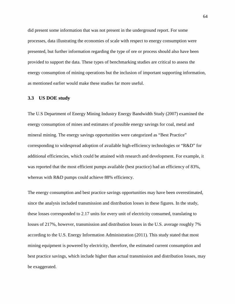
64

did present some information that was not present in the underground report. For some

processes, data illustrating the economies of scale with respect to energy consumption were

presented, but further information regarding the type of ore or process should also have been

provided to support the data. These types of benchmarking studies are critical to assess the

energy consumption of mining operations but the inclusion of important supporting information,

as mentioned earlier would make these studies far more useful.

3.3 US DOE study

The U.S Department of Energy Mining Industry Energy Bandwidth Study (2007) examined the

energy consumption of mines and estimates of possible energy savings for coal, metal and

mineral mining. The energy savings opportunities were categorized as “Best Practice”

corresponding to widespread adoption of available high-efficiency technologies or “R&D” for

additional efficiencies, which could be attained with research and development. For example, it

was reported that the most efficient pumps available (best practice) had an efficiency of 83%,

whereas with R&D pumps could achieve 88% efficiency.

The energy consumption and best practice savings opportunities may have been overestimated,

since the analysis included transmission and distribution losses in these figures. In the study,

these losses corresponded to 2.17 units for every unit of electricity consumed, translating to

losses of 217%, however, transmission and distribution losses in the U.S. average roughly 7%

according to the U.S. Energy Information Administration (2011). This study stated that most

mining equipment is powered by electricity, therefore, the estimated current consumption and

best practice savings, which include higher than actual transmission and distribution losses, may

be exaggerated.

65

The energy consumption data for the U.S. study (2007) were derived from a model using mining

parameters that described the ore body characteristics as inputs, rather than using data from

existing operations. The model then listed the equipment requirements, the number of units of

each piece of equipment, and the estimated daily operating time for each unit of equipment for a

hypothetical mining operation. Using this information with an assumed production rate for the

hypothetical mine, it was possible to calculate the specific energy consumption per short ton of

material handled. This approach was repeated for different mining methods as well as for

different commodities to generate a set of data samples. However, the model did not incorporate

beneficiation and processing, therefore, the projected energy consumption figures for these

production stages were provided by industry experts. Subsequently, the weighted average

specific energy consumption was calculated for all U.S. mines for each commodity group, by

using knowledge of their mining methods and production rates. Finally, the annual energy

consumption for each commodity group was estimated by using the annual production of each

commodity group across the U.S. While this approach provides a useful estimate of energy

consumption in the U.S. mining industry, there is a definite need to validate these figures with

actual data from operating mines, to reduce the uncertainties associated with this analysis. In

addition, benchmarking several operations would be necessary, as multiple factors that

significantly influence energy consumption were omitted, such as mining depth, mining method

and geology.

3.4 Statistics Canada

Canadian energy consumption data is collected by Statistics Canada via various surveys and

censuses which are made available in reports and CANSIM tables. Caution should be exercised

66

when consulting the published reports since data may be revised post-production. Therefore it is

advised to consult the CANSIM tables to obtain the most recent data.

Relevant reports, published on an annual basis from the Canadian mining sector include

(Statistics Canada var.a, Statistics Canada var.c): i) Report on Energy Supply and Demand in

Canada (RESD), and ii) General Review of the Mineral Industries (or Annual Census of Mines).

The corresponding annualized data from these reports is available in the following CANSIM

tables (Statistics Canada 2013): 128-0016 Supply and demand of primary and secondary energy

in terajoules, 153-0032 Energy use by sector in terajoules, and 128-0006 Energy fuel

consumption of manufacturing industries in gigajoules.

CANSIM table 128-0016 gives the total Canadian energy use by source from 1995 to 2011, as

well as by sector and sub-sector. Unfortunately, the level of disaggregation is not sufficient to

conduct an in-depth analysis. For example, energy use for the mining sector is identified by

“Total mining and oil and gas extraction” and no further disaggregation of data is available. This

data may be useful in some instances, but if trends in energy efficiency are to be examined, it

would be difficult to do because of the number of sub-sectors included in this group. It was

indicated that this table replaced CANSIM table 128-0009, which contained data from 2002 to

2009, but a note specified that comparison of these tables should be undertaken with caution.

Furthermore, for mining sector data it was also revealed that some sub-sectors were excluded

from the dataset prior to 2004, therefore a historical analysis would also be difficult to complete.

Annual energy use by sector from 1990 to 2008 is provided in Table 153-0032, where data

pertaining to the mineral industry, disaggregated according to the North American Industry

Classification System (NAICS), is available for i) oil and gas extraction, ii) coal mining, iii)

67

metal ore mining, and iv) non-metallic mineral mining and quarrying, as well as v)

miscellaneous non-metallic mineral product manufacturing, and vi) primary metal

manufacturing. This level of disaggregation is better than that of Table 128-0016, but is only

useful when corresponding data that could be used to explain variation in energy use are

available. This includes: production, ore grade, mining depth and stripping ratio. Disaggregated

data by energy type (i.e. electricity, fuel, gas, etc.) could also be useful.

Mining production data from 1996 to 2006 can be accessed in the Annual Census of Mines

(ACM), published by Statistics Canada, under the direction of Natural Resources Canada

(Statistics Canada var.a). The reports provide provincial mineral production data for metallic and

non-metallic minerals, as well as national energy use by source for mineral industries excluding

fuels. Used together, the energy and production data from this report can be used for an industry-

wide energy analysis to examine energy use per tonne of product, however it may not be possible

to assess efficiency trends because these values would be affected by: i) changes in ore grade

over time, and ii) structural shifts within the industry. An analysis based on the various

commodities or sub-sectors could not be completed, because the energy data was aggregated to

the sector level only. The reports also provided production costs such as wages and salaries,

materials and supplies, as well as fuel and electricity for the minerals industry and selected

manufacturing industries. This information could be used to assess the relative costs of

production within the mining sector.

Disaggregated information pertaining to the smelting and refining sector was collected via

Statistics Canada’s Annual Survey of Manufacturers. Annual data was available in CANSIM

table 128-0006 Energy fuel consumption of manufacturing industries in gigajoules, by NAICS

(Statistics Canada 2013) from 1995 to 2011, and was disaggregated by sub-sector. This level of

68

detail could be useful for comparing and assessing energy consumption from these sub-sectors,

however, an efficiency analysis would require more data, such as production or throughput.

Statistics Canada is a valuable resource for energy use and production data from the mineral

sector. However, for an energy efficiency analysis, significant effort would be required to

construct a useful dataset, with consistent boundary definitions between sub-sectors for each

metric (i.e. energy use, production, etc.). Furthermore, an analysis at the sub-sector level would

be the most granular that could be achieved, since energy data are not published by commodity.

3.5 Natural Resources Canada

3.5.1 Canadian Minerals Yearbook

Natural Resources Canada compiles information, focused on the non-fuel mineral industry, from

surveys and Statistics Canada data in an annual report entitled, Canadian Minerals Yearbook

(CMY) (Natural Resources Canada 2011b). Reports, available online, have been published for

census years from 1944 to 2011 and include production, price, export and import data for various

minerals. Earlier Canadian mineral production data is also available, dating as far back as 1858

for gold (Canada Department of Trade and Commerce 1945, Canada Department of Trade and

Commerce 1939), however, the corresponding energy consumption data is absent, which is

required for a historical energy efficiency analysis.

The content of the Canadian Minerals Yearbook reports has changed over time, therefore, not all

information is available for each year. For example, since 1956 energy consumption data was

included in the reports, which consisted of electricity consumption in kWh and other fuels in

dollar values, disaggregated by sub-sector for metal mining, industrial minerals and fuels. This

69

information only allowed an energy efficiency analysis to be done for electricity, since there was

no way to convert the aggregated other fuels to energy units. In 1957, the reports began listing

disaggregated energy consumption data by source for metals, smelting and refining, industrial

minerals and mineral fuels. However, later on the reports excluded smelting and refining as well

as fuel minerals data. The same data was also included in the Annual Census of Mines. An

energy efficiency analysis using the data from the CMY can provide an industry perspective but

assessment at the commodity level is not possible when only aggregated energy data is available.

3.5.2 Energy Use Data Handbook Tables 1990-2010

Natural Resources Canada’s Office of Energy Efficiency publishes the Energy Use Data

Handbook Tables, which contain data showing annual energy use, greenhouse gas emissions and

energy prices (Natural Resources Canada ca. 2013a). These tables, which can be downloaded in

spreadsheet format, contain: residential, commercial / institutional, industrial, transportation, and

total end-use data as well as information on electricity generation. Mining industry data is found

in the industrial section of the publication and was obtained from Statistics Canada and the

Canadian Industrial Energy End-use data and Analysis Centre (CIEEDAC). These tables provide

the annual energy consumption of the Canadian mining industry, however, without production

data this information cannot provide any insight into energy efficiency. The tables do provide the

annual energy intensity for industries. Unfortunately, since the units are not consistent,

comparing the various mining sub-sectors is not straightforward. For example, there are eight

commodities which are included in the mining sector, of which six report energy intensity in

MJ/tonne, one sector uses MJ/$2002- GO (Gross Output) and the last one uses MJ/ $2002 GDP

(Gross Domestic Product). However, since energy consumption and GDP are provided for each

70

of the commodities, it was possible to calculate all of the mining sub-sector energy intensities in

MJ/ $2002 GDP, which are shown in Figure 13.

Since the GDP incorporates commodity prices, the energy intensities provided (Natural

Resources Canada ca. 2013a) cannot be used to identify energy efficiency trends in the mining

industry. For example, if we consider two years where production and energy consumption

remain stable, a rise in the price of a commodity for one year would increase the GDP, but the

resulting energy intensity would be lower when utilizing MJ/GDP units.

Figure 13: Energy intensity, expressed as MJ/$2002 GDP for selected Canadian mining sectors (Natural Resources Canada ca. 2013a)

However, the tables do include energy intensity per unit of output for six mining sub-sectors,

which are illustrated in Figure 14.

0

10

20

30

40

50

60

70

80

90

100

1990 1995 2000 2005 2010

Ener

gy In

tens

ity (M

J/$2

002

GDP)

Copper, Nickel, Lead and Zinc Mines Iron Mines Gold and Silver Mines

Other Metal Mines Salt Mines Potash Mines

Other Non-Metal Mines Upstream Mining

71

Figure 14: Energy intensity in MJ/tonne ore (metals) and MJ/tonne product (non-metals) for selected Canadian mining sectors (Natural Resources Canada ca. 2013a)

It can be observed from Figure 14 that the energy intensity of potash mining is approximately

one order of magnitude higher than the other types of mining included in the analysis. Further

investigation revealed that the units for the commodities are not consistent. For example, salt and

potash production is based on the amount of final product, whereas the other commodities

include the amount of ore milled. The comparison is biased because the energy intensity of the

metals is calculated using the amount of final product and waste. However, for the non-metals

sector, only the final product amount is used to calculate the energy intensity. It appears that the

potash mines are more energy intensive, but this data does not provide sufficient information to

properly assess the energy efficiency between metal and non-metal production. A proper

10

100

1000

10000

1990 1995 2000 2005 2010

Ener

gy In

tens

ity (M

J/to

nne)

Copper, Nickel, Lead and Zinc Mines (MJ/t ore) Iron Mines (MJ/t ore)Gold and Silver Mines (MJ/t ore) Other Metal Mines (MJ/t ore)Salt Mines (MJ/t product) Potash Mines (MJ/t product)

72

comparison between commodities, normalized by consistent units, would help identify where

energy management efforts should be focused within the mining sector.

3.5.3 Comprehensive Energy Use Database Tables

Natural Resources Canada publishes energy consumption data, disaggregated by type for the

following sub-sectors within the Canadian mining sector (Natural Resources Canada nd):

• copper, nickel, lead and zinc mines

• iron mines

• gold and silver mines

• other metal mines

• salt mines

• potash mines

• other non-metal mines

• upstream mining.

The tables also include energy intensity for these sub-sectors but suffer from the same issue as

the Energy Use Data Handbook Tables; the units used to measure production are not consistent

between commodities. Tonnes of ore milled were provided for the metal mines, tonnes of

product were given for salt and potash whereas GDP was presented for other non-metal mines

and upstream mining.

The value from these tables was the breakdown of energy use by type (electricity, natural gas,

diesel…) which could permit an assessment of historical trends within a sub-sector, or a

73

comparison between different sub-sectors. However, insufficient information is available for a

comprehensive assessment. For example, energy intensity for the copper, nickel, lead and zinc

mines increased by 7% from 1990 to 2012, but electricity use per tonne of ore milled decreased

by 11% whereas an increase of 74% was observed for diesel intensity, as was shown in Figure 6.

This may be explained by structural shifts within the sub-sector such as new mines employing

open-pit mining methods thus using more diesel but not requiring ventilation. Alternatively, this

could also be explained by the use of larger hauling equipment and improvements or energy

conservation efforts adopted in underground ventilation systems. Thus further disaggregation by

mine type (underground vs open-pit) may provide a better understanding of the energy trends

within the sub-sectors.

3.6 Canadian Industrial Energy End-use Data and Analysis Center (CIEEDAC)

CIEEDAC, a research group at Simon Fraser University in British Columbia analyzed and

published reports focussing on Canadian industrial energy use for various sectors (Canadian

Industrial Energy End-use Analysis Center (CIEEDAC) var.). Reports specific to the Canadian

mining industry were prepared and included annual energy use and indicators for metal mines,

non-metal mines as well as the smelting and refining sub-sector, with data gathered from various

Statistics Canada and Natural Resources Canada sources. In addition, the group maintains a

database that contains energy by source and production data, disaggregated by NAICS (Canadian

Industrial Energy End-use Analysis Center (CIEEDAC) 2013).

Composite intensity indicators were used in CIEEDAC reports to aggregate specific energy

consumption values (i.e. energy per tonne milled) for the mining sector. These indicators were

designed to remove the influence of structural shifts within an industry by weighting the energy

74

use of a sub-sector, normalized against its share of the total sector energy consumption. Although

structural shifts within a sector could be misinterpreted as a change in energy efficiency, the use

of the composite indicator failed to include other factors that could influence energy

consumption in the mining sector. For example, mines extracting ore from deeper levels

consume greater amounts of energy, which can mask any improvements achieved by energy

conservation efforts, as demonstrated by Goldcorp’s Musselwhite mine example in Section 3.1.6.

Therefore the inclusion of such factors needs to be considered to quantify energy efficiency

trends. Admittedly, some data, such as mining depth, are typically not available.

3.7 Other sources

Statistics Canada has also published Historical Statistics of Canada, of which mining is a

separate section (Statistics Canada 1999). The data contained in this report includes the same

type of information listed in the CMY and the ACM but dates back to 1923.

Two other reports pertaining to the mining sector were published by Statistics Canada; the Metal

Ore Mining Report covers 1996 to 2005 and the Non-metal Mines Report only covers 1996 and

1997 (Statistics Canada var.b, Statistics Canada var). These publications include the same type of

data as was in the CMY and ACM. The data is more disaggregated in some cases, but contains

several confidential values that were excluded from the tables. Although the data in these reports

is disaggregated, a complete analysis cannot be completed, because of the exclusion of

confidential data. Furthermore, the short publication periods also limit the scope of analysis of

these data and prohibit any analysis of recent trends.

75

3.8 Issues with Canadian mining data

Comparison of the data from CANSIM tables 128-0006 and 153-0032 revealed that the values

were slightly different. For example, energy consumption from Primary metal manufacturing in

2008 corresponded to 503,793,887 GJ in Table 128-0006 and 512,104 TJ in Table 153-0032.

Presumably, the difference may be due to different boundary definitions of the sector or by

varying data collection or conversion methods employed by the respective surveys, but the final

reason for this is unclear.

Over the years, sector and sub-sector definitions have been revised with the introduction of the

NAICS. Even after the NAICS was defined, some reports excluded certain sub-sectors from their

reports and data tables. For example, energy consumption from the mining industry presented in

RESD excluded two sub-sectors and part of another prior to 2004. Although the changes may be

considered marginal, this could introduce a level of uncertainty when conducting a historical

analysis.

Energy consumption by type was available in the Canadian Minerals Yearbook (for metals, non-

metals and total industry) as well as in the Annual Census of Mines (for mineral industries

excluding fuels). Although the data in these publications are comparable, the ACM indicates that

smelting and refining is included whereas the CMY does not provide a clear indication of its

boundary definitions, which introduces uncertainty when using this information in an analysis.

CIEEDAC defines the mining industry by using the NAICS but excludes quarries, sand, gravel,

clay and ceramic minerals as well as oil, gas and coal. This may make the assessment of data

difficult during comparisons with other mining sector publications which may have included all

sub-sectors from the mining industry, as defined by the NAICS. Therefore, it is imperative when

76

comparing or combining information from various sources to fully understand their boundary

definitions.

The references examined seemed to be circular. Data was collected by Statistics Canada and

from Natural Resources Canada surveys, and published in reports and CANSIM tables. Mining

related energy and production data from these sources were then assembled by CIEEDAC into

reports and a database. Subsequently, the CIEEDAC reports were referenced in Natural

Resources Canada’s Energy Handbook Tables, which also sourced information from Statistics

Canada’s RESD. However, the ‘same’ data listed in these sources are not always identical. Table

4 shows examples of these discrepancies.

Table 4: Comparison of reported energy consumption from various sources

Sector Year NRCan

Handbook

tables

CIEEDAC RESD CANSIM

128-0016

Iron mines 1990 39.75 PJ 42,352 TJ N/A N/A

Iron mines 2010 45.41 PJ 41,314 TJ N/A N/A

Total industrial 2008 3,283 PJ 2,565 PJ 2,280,195 TJ 2,392,115 TJ

Although some of the differences between the values in Table 4 could be considered minor, these

differences undermine confidence in either source as being definitive. A cursory investigation

revealed that these discrepancies were caused by the different aggregation methods used to

generate the reports.

77

The construction of a complete dataset for an energy efficiency analysis of the minerals industry

was not possible by only using information from a single source. However, CIEEDAC compiled

and presented the most comprehensive set of statistics, from an energy efficiency analysis

perspective. Furthermore, the data presented by CIEEDAC was disaggregated according to the

NAICS, and included energy consumption by type as well as production. This level of

disaggregation was found to be the most useful, but the data could not be independently verified,

because even though the data are still being collected by Statistics Canada, they are not being

published.

Due to the varying levels of disaggregation, different sector definitions, different date ranges and

discontinued surveys from available resources, conducting an in-depth analysis of energy

efficiency in the mining industry is not as straightforward as it should be. A proposed solution

would be to: i) ensure the use of the NAICS in all reports and tables to clearly define the

boundaries of the presented data, and ii) provide energy by source and production data,

disaggregated to 6-digit NAICS format, as is the case with CIEEDAC. This data is suitable for

an analysis at the sub-sector level, but to assess the performance of individual mines, publication

of additional support variables is needed. This was illustrated with the Musselwhite Mine case

study in Section 3.1.6.

3.9 Proposed solution for improving reported energy- related data from the

mining sector

The review of data relating to energy use in the mining sector has revealed deficiencies. As this

information may be used to inform policy makers and to provide guidance for industry priorities

it is imperative that these shortcomings are addressed. The following recommendations are

78

proposed for moving forward for gaining a better understanding of energy use and trends within

the mining sector.

Adoption of one standard for publication of sustainability reports would reduce confusion and

effort requirements to comply with multiple frameworks. As the UN Global Compact, the ICMM

and TSM are all linked either directly or indirectly to the GRI it appears that the GRI standard

may the one of choice. Furthermore, this framework includes a comprehensive list of indicators

and separate guidance for the mining industry with the Mining and Metals Sector Supplement

(MMSS). However, it is suggested that this guidance document be revised to include reporting of

energy use from individual sites, disaggregated by energy type. The addition of reporting support

variables such as mine depth (for underground mines) and hauling distances (for open-pit mines),

production (amount of material processed), proportion of ore mined from underground and open-

pit mining, as well as heating and cooling requirements (reported as heating degree days and

cooling degree days) would benefit those consulting these documents as well as good performers

within the mining industry. Disaggregation of data on a quarterly basis is recommended to

permit assessment of seasonal variability and inclusion of historical data would permit an

assessment of performance from individual mine sites. It is also suggested that reporting of

energy conservation measures are included in such reports to enhance or accelerate

dissemination of best practice.

Alignment of the reporting criteria for sustainability reports and government publications to limit

any additional effort required by industry is suggested. The data could be aggregated to the sub-

sector level, which could allow comparison between commodities. Inclusion of the same support

variables as those proposed for sustainability reports is suggested however, composite indicators

that use weighting factors as those developed by CIEEDAC would be required for use at the sub-

79

sector level. However, reporting production as total material processed for all sub-sectors is

suggested so that a fair comparison can be made between the various commodities extracted in

Canada. Table 5 summarizes the proposed recommendations for sustainability and government

reporting. It should be noted that the shaded cells correspond to currently reported criteria.

Table 5: Recommendations for improved reporting

Sustainability reports Government reports

Disaggregation level individual sites sub-sector

Energy use by type by type

Support variables mine depth / hauling distance

production

proportion of ore mined underground vs open-pit

HDD, CDD8

mine depth / hauling distance

production

proportion of ore mined underground vs open-pit

HDD, CDD

Presentation of data quarterly quarterly

Historical data 5 years 20 years

Other energy conservation projects

It can be observed from Table 5 that some of the recommendations are currently implemented in

government reports. Although some companies choose to report energy use and/or production in

sustainability reports these indicators are not required for compliance with reporting standards.

8 HDD: heating degree days, CDD: cooling degree days

80

Inclusion of the proposed additional information may clarify energy performance and provide

insight on focus areas for future improvements.

81

4 A review of existing energy audit methodologies and guidelines

Energy audits are an underpinning element in energy management; they provide the information

to understand how, and when energy is used, which is subsequently relied upon to identify

potential savings. This section aims to describe different methodologies employed to conduct

energy audits, as well as their advantages and disadvantages.

The amount of detail and energy conservation measures identified in an energy audit depends on

the audit level; a higher level would include a more detailed analysis. The American Society of

Heating, Refrigeration, and Air-Conditioning Engineers (ASHRAE) define three energy audit

levels:

• Level 1: Also known as a walk-through audit, where energy conservation measures are

recognized with minimal or no measurements. This type of audit can serve to identify

priority focus areas for the next energy audit level.

• Level 2: Consists of an energy survey and analysis stage where metering is carried out to

gather sufficient information to assess the economic viability of any proposed energy

conservation measures.

• Level 3: Large investments are usually included in this type of audit, which can involve

energy modeling for a more in depth analysis (Rosenqvist, Thollander et al. 2012, The

Association of Energy Engineers nd, Thumann, Mehta 2008).

Three additional audit types were defined by the Association of Energy Engineers as follows:

• Benchmarking audit: This type employs an energy use index (EUI) or energy cost index

(ECI) to compare the energy performance of separate facilities. The EPA Energy Star

82

Portfolio Manager was designed to benchmark energy, water, and carbon emissions for

buildings (The Association of Energy Engineers nd, United States Environmental

Protection Agency 2015). This platform has also been adopted by the Canadian

Government to benchmark commercial and institutional buildings (United States

Environmental Protection Agency 2015, Natural Resources Canada 2014).

• Investment grade audit: With this type, a risk weighting is incorporated into the economic

assessments used in Level 2 and Level 3 audits (The Association of Energy Engineers

nd).

• Master audit: This type of audit would be used for construction and future operation of a

system, and would consider codes and standards, maintenance schedules and equipment

inventory (The Association of Energy Engineers nd).

Energy audits can be conducted in three phases, illustrated in Figure 15.

83

Figure 15: Energy audit phases (Capehart, Turner et al. 2012, Doty, Turner 2009)

• define scope • analyze energy bills • revise tariffs • review facility layout • gather production and weather data • obtain equipment inventory and operating schedule • determine focus areas for survey measurements

Preparation

• meet with management and maintenance personel • conduct interviews to gather facility and

operational information • conduct a walk-through tour • acquire detailed data for facility and equipment • develop an energy balance • analyze data to identify energy conservation

opportunities • prepare audit report • develop action plan for implementation of energy

conservation opportunities

Survey and analysis

• form energy action committee and define goals • assess and rank energy conservation opportunities • implement energy conservation opportunities

Implementation of

recommendations

84

The type of measurements that should be conducted during the survey phase of the energy audit

corresponded to: voltage, amperage, power factor, flowrate, temperature, light intensity, leakage,

and combustion efficiency. These measurements can then be used in the analysis stage to

estimate: the energy consumption of equipment, energy waste, and energy associated with

material flows.

Energy audits can be performed using a bottom up, or a top down methodology, or a

combination of these approaches. In a bottom up audit, data for individual items are gathered and

aggregated to determine the total consumption of a facility. Conversely, in the top down energy

audit, data is gathered at the highest echelon within the defined energy audit boundary to identify

priority focus areas then the assessment proceeds to the next level of granularity. Each auditing

methodology will be considered in greater detail in the following sections.

4.1.1 Top down energy audit

Rosenqvist et al (2012) presented an energy audit methodology for industrial facilities

combining a top down technique with an iterative process. The proposed methodology,

developed at Linkoping University, in Sweden has been used to carry out roughly 500 energy

audits that comprised a survey, an analysis, and an energy conservation stage.

The method was referred to a top down process since the audit began with a wide scope that

aimed to highlight focus areas where additional data and analysis may ensue. The iteration step

corresponded to returning to the survey stage of the process with the identification of information

gaps during the analysis phase, which continued until sufficient information was gathered to

identify potential energy conservation initiatives. Figure 16 shows an overview of the top down

energy audit process described in Rosenqvist (2012).

85

Figure 16: Overview of top down energy audit (adapted from (Rosenqvist et al., 2012)

Facility

Activity or Process

Activity or Process

Identify priority areas

Conduct survey

Analyze data

Identify potential savings

Energy (electricity, fuels…)

Information gaps

86

The top down energy audit methodology proposed the use of six steps (Rosenqvist, Thollander et

al. 2012):

1. Gather information by activity or process: this included a review of energy bills, facility

drawings, and production schedules, among others. This stage also led to the

identification of focus areas for the next steps.

2. Conduct the survey by visiting the facility during production periods: this step was used

to collect data via installation of meters and data loggers or other measuring devices.

During this step it was also suggested to discuss with personnel to gain a better

understanding of the facility and the processes.

3. Gather additional survey data by visiting the facility during non-production hours: this

step would permit the identification of potential sources of energy waste, such as idling

equipment.

4. Analyze the data to allocate energy consumption and create a balance: this step

corresponded to using the data gathered from the previous steps to determine the energy

use from different processes which were identified as priority focus areas. The energy

balance ensured that all energy use within the defined boundaries was allocated.

5. Identify potential energy savings and create new energy balance: this step was used to

illustrate the potential impact from the various energy conservation measures identified

during the audit.

6. Meet with industry representatives: the purpose of this step was to communicate the

survey findings and discuss a potential path forward for implementation of energy

conservation measures.

87

Use of the top-down energy audit presents the disadvantage that with focus in specific areas of

the facility or process, detailed energy consumption from all end-uses is not quantified.

However, this may also represent an advantage of this method since the examination of priority

areas may correspond to those with the greatest potential for energy savings.

4.1.2 Bottom up energy audit

In a bottom up audit, extensive metering, modeling or estimation is undertaken to determine the

energy consumption of the individual end-uses within the boundaries of the energy audit.

Although there is no substitute for metered data, metering all of the equipment may not be

financially feasible. An alternative may be to monitor major energy consuming items and energy

consumption for non-metered equipment could be projected from estimates of hours of operation

and equipment loading (Vogt 2003) or modeling. However, this approach would introduce

uncertainty with the audit values and results. The bottom up method requires substantial

investment and commitment for purchasing and installing the meters, or for modeling and

estimating energy use, and for analyzing the collected data.

An alternative method called the energy balance was developed to simulate the bottom up energy

audit (Pawlik, Capehart et al. 2001). An overview of the steps involved in the energy balance

methodology is illustrated in Figure 17.

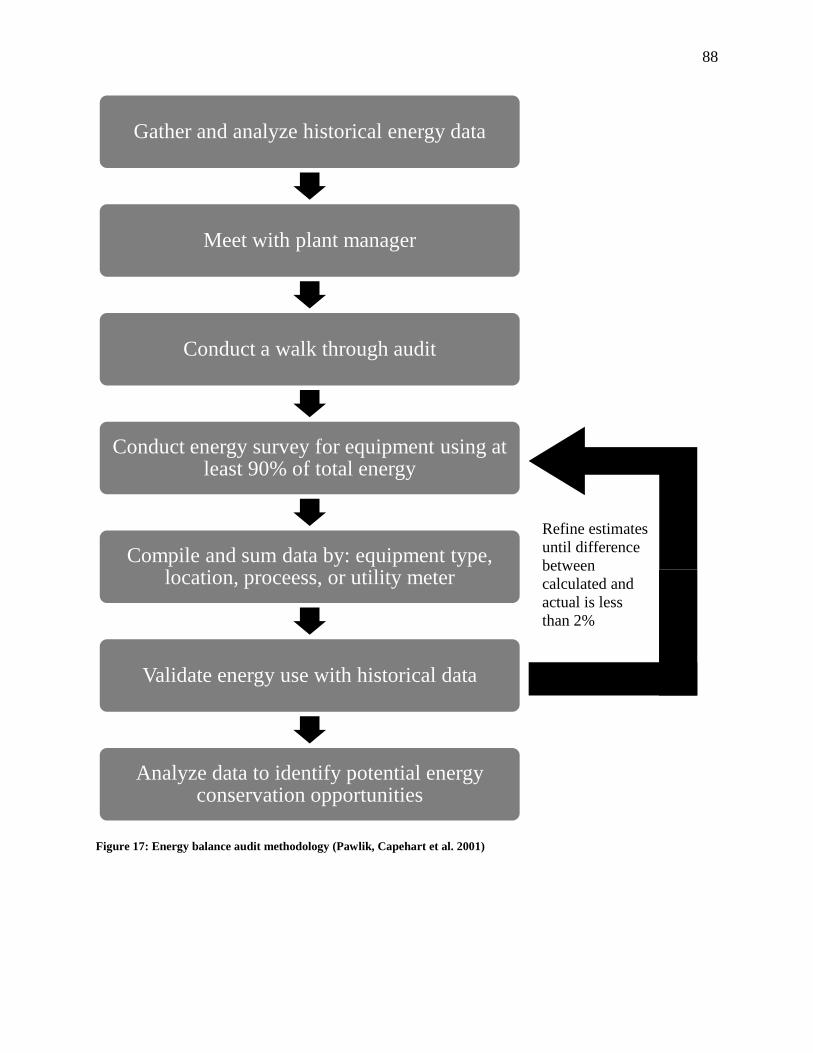
88

Figure 17: Energy balance audit methodology (Pawlik, Capehart et al. 2001)

Gather and analyze historical energy data

Meet with plant manager

Conduct a walk through audit

Conduct energy survey for equipment using at least 90% of total energy

Compile and sum data by: equipment type, location, proceess, or utility meter

Validate energy use with historical data

Analyze data to identify potential energy conservation opportunities

Refine estimates until difference between calculated and actual is less than 2%

89

The principle behind the energy balance is to improve the accuracy of the estimated data during a

bottom up energy audit by ensuring that the sum of the individual end-uses corresponded to the

total consumption at the facility. In the absence of extensive continuous metering, as could be

involved in a bottom up energy audit, the energy balance methodology allows the auditor to

estimate the energy use from individual equipment that would account for a minimum of 90% of

total facility energy use. This includes either data or estimates of the following (Pawlik, Capehart

et al. 2001):

• annual operating hours for the facility

• utilization factor for the equipment (fraction of total annual operating hours for which a

specific piece of equipment was in operation)

• rated power of equipment

• equipment efficiency

• motor load factor (fraction of rated power at which a piece of equipment was operated)

• diversity factor (probability of equipment running during the facility’s peak demand).

Subsequently, the data from the individual equipment is used to calculate the annual energy

consumption, as well as the minimum and maximum demand for the entire facility. These figures

are then compared to historical billing information to validate the assumptions or estimates used

in the audit. If the calculated and actual values differ by more than a few percentage points, it is

suggested to review the equipment inventory to ensure that it was complete. Further actions to

reconcile the data consist of understanding of the equipment and its use, as well as understanding

the utility invoices. It was also recommended to adjust the load factor, the utilization factor, or

90

the diversity factor depending on the situations exemplified in Table 6, to ensure that the

calculated and actual energy and demand values were within 2% of each other.

Table 6: Recommended adjustments for reconciling energy audit data (Pawlik, Capehart et al. 2001)

Demand Energy Adjustments

calculated < actual calculated < actual Increase load factor for some motors

calculated > actual calculated > actual Decrease load factor for some motors

calculated = actual calculated < actual Increase utilization factor for some

equipment

calculated = actual calculated > actual Decrease utilization factor for some

equipment

calculated < actual calculated = actual Increase diversity factor for some

equipment

calculated > actual calculated = actual Decrease diversity factor for some

equipment

calculated > actual calculated < actual Decrease diversity factor and increase

utilization factor for some equipment

calculated < actual calculated > actual Increase diversity factor and decrease

utilization factor for some equipment

The final step in the energy balance methodology consists of data analysis to identify potential

energy conservation measures.

91

4.1.3 Hybrid top down / bottom up energy audit

A hybrid method combining the top down and bottom up methodology was used by Bennett and

Newborough (2001) to conduct a city-wide energy audit. The task began using the top down

approach to separate the city into sectors and sub-sectors, illustrated in Figure 18.

Figure 18: Sector and sub-sector classification from top-down method (Bennett, Newborough 2001)

Subsequently, the energy consumption of the components within each sub-sector was estimated

with the use of metered data, using inventory or census information with energy intensity factors,

or by employing mathematical models. These values were summed to determine the energy use

allocated to each sub-sector, which corresponded to the bottom up portion of the method. The

sub-sector data was then aggregated to estimate the corresponding sector energy use, which was

summed to approximate the city-wide energy consumption. Bennett and Newborough (2001)

suggested the implementation of a checking procedure to minimize discrepancies identified

during the aggregation process by refining assumptions. This checking procedure could entail an

• dwellings • appliances and lighting Domestic

• standard industrial classification sub-sectors

Industrial and commercial

• standard industrial classification sub-sectors Municipal

92

energy balance whereby comparison of sector or sub-sector estimates with actual energy use is

employed.

The level of detail from this hybrid method does not compare with that of the bottom up energy

audit where all end-use consumption is metered but it does provide an indication for priority

focus areas for energy conservation measures. However, it was indicated by the authors that

setting energy conservation targets was not straightforward since some of the values determined

during the audit were estimated from average or typical energy use and the penetration rate of

energy efficiency measures was not known. Thus proposing appliances or equipment

replacement with more efficient units may not yield the anticipated energy savings if most of the

actual components in use were already classified as high efficiency.

The energy audit methods presented in this section were included to illustrate different

approaches that can be undertaken to conduct energy audits. Although there is not a standardized

methodology, there were some common items between the reviewed procedures that could be

considered good practice. For example, all methods included a balancing step to ensure that the

sum of energy use at the bottom level corresponded to the energy from the top level. The

reviewed methodologies also proposed an iterative step to refine the energy balance between the

top and bottom energy use. Furthermore, all proposed a historical energy audit for at least a 12

month period to assess the seasonal variability of energy consumption.

The main benefit of the top down method and the hybrid method is that it permits identification

of areas for conducting a more detailed investigation. This would entail less time and effort, thus

less cost than an exhaustive bottom up audit but there may be some missed opportunities for

energy conservation in areas that were ignored. Conversely, while the bottom up method does

93

provide a detailed understanding of energy use at a granular level, a larger investment is required

regardless if the end-use consumption is metered or estimated. Continuous monitoring of all end-

uses would require purchase, installation and maintenance of meters, as well as data storage

capacity and a system for monitoring and analyzing the data. Although the installation of meters

was not a requirement in any of the methods reviewed in this section, the use of metered data

would reduce the level of uncertainty in an energy audit.

The bottom up method yields a great amount of detail regarding individual end-use energy

consumption but the amount of data may be overwhelming for facilities with a large amount of

equipment, which could consequently hinder the data analysis and identification of energy

conservation measures. Although the energy balance method lacks the accuracy of continuous

metering, it does provide the same level of detail as the bottom up method and may be used to

identify loads that should be monitored. The energy balance methodology presented practical

guidelines that could be used for balancing the calculated energy use with the actual value, which

the other methods suggested as an essential step but did not provide guidance.

Selection of an appropriate method is not straightforward but should be based on the scope and

goals of the audit and could comprise a combination of the reviewed methodologies.

4.2 Industrial energy audit guidelines

The top-down and bottom-up methods illustrate general approaches for conducting energy audits

that could be applicable to different sectors including: residential, commercial or industrial.

Government agencies have developed resources for assisting with energy audits considering

specific applications to industrial facilities. Some examples were chosen and a brief overview of

each is presented in the following.

94

4.2.1 Energy Savings Toolbox

The Energy Savings Toolbox was developed by the Canadian Industry Program for Energy

Conservation (CIPEC) and provides detailed guidelines for conducting an energy audit in

industrial facilities (Natural Resources Canada 2009). Inclusion of checklists and Microsoft

Excel tools facilitate the energy management process.

The guidance adopted a process flow based on the energy audit phases outlined in Figure 15, but

suggested that a condition survey, which corresponded to the walk through step, be undertaken

as the first step in the audit. The purpose of this step was to help guide the definition of the scope

and boundaries by identification of focus areas.

The proposed condition survey employed a checklist that used a rating system to identify and

rank priority focus areas for energy management. Checklist examples were provided for common

utilities and types of areas common to industrial sites (e.g. walls, doors, compressors, boilers,

etc.) but custom checklists would have to be prepared for site specific uses. For example, in an

underground mine, checklists for pumps, hoists, ventilation systems, or mobile equipment would

have to be developed. A checklist was also included to assist with the development of the audit

mandate and scope.

The Energy Savings Toolbox included a guidance section and a spreadsheet aimed to assist with

understanding energy use and billing tariffs. Conversion of all energy sources to common units

was suggested to facilitate comparison. Use of the tool provided may be of limited use for mines

since it failed to include transportation fuel, which could correspond to a significant proportion

of total energy especially for open-pit mines.

95

A comparative analysis was suggested to benchmark and assess energy performance against

internal and external facilities. Regression analysis was used to determine a facility’s baseline

energy consumption from the relationship between energy use and one driver but the tool only

has the capability of including one factor of influence. Furthermore, a cumulative sum of

differences (CUSUM) analysis was included to examine the difference between the baseline and

the actual energy use, which is illustrated in Figure 19 where ‘Variance Energy’ values indicated

in brackets correspond to periods of better than expected energy performance, which are

illustrated by the negative values on the plot.

96

Figure 19: Screenshot of CUSUM analysis tool from Energy Savings Toolbox (Natural Resources Canada 2009)

The spreadsheet also contains a tab that allows the user to define the period of best performance,

which can assist in setting an energy conservation target. Alternatively, a target can also be

defined by the baseline energy use established from all data. For example, a target of 5% overall

energy reduction could be set but the target should not exceed the facility’s best performance

because may this may not be attainable. Figures are automatically produced for visual

interpretation of the data.

97

A section in the guidance document and a spreadsheet were also included in the Toolbox to assist

with the interpretation of demand profiles. A correlation between demand and operating

schedules was suggested to determine the equipment or activities that are contributing to the

facility load. This section also explained how to analyze demand profiles to identify savings

arising from load shifting, load shedding, or shutting down idling equipment during non-

production periods. Figure 20 shows the Demand Profile Analysis tool.

Figure 20: Screenshot of Demand Profile Analysis tool from the Energy Savings Toolbox (Natural Resources Canada 2009)

98

A tool and guidelines were provided to determine the electrical load inventory consisting of a

breakdown of energy and demand from different categories. This was achieved using equipment

rating, operating hours, and a diversity factor. Suggestions for energy conservation opportunities

that may arise from analysis of the load inventory were included. This section of the guidelines

also described how to map thermal energy flows and promoted the use of a Sankey diagram to

illustrate these and to ensure that there is an energy balance between inflows and outflows.

A three step procedure was proposed in the guidelines to identify energy conservation

opportunities as follows:

1. ensure that energy usage was matched to the requirements,

2. maximize energy efficiency, and

3. optimize the energy supply via heat recovery, heat pumps, cogeneration, renewable

energy systems, fuel switching, or purchase optimization.

Evaluation of the economic viability of the proposed energy conservation measures was

suggested using a discounted cash flow model, which was included in the toolbox. The model

provided an estimate of the net present value, internal rate of return, simple payback and GHG

reduction for the proposed energy savings.

The final section of the guidance document provided a template that could be used to prepare an

energy audit report.

The Energy Savings Toolbox comprised comprehensive, systematic guidance and the tools to

conduct an energy audit and perform an analysis to identify energy conservation opportunities.

99

4.2.2 Industrial Energy Audit Guidebook – Guidelines for Conducting and Energy

Audit in Industrial Facilities

The Industrial Energy Audit Guidebook, sponsored by the U.S. Department of Energy, was

developed based on the framework outlined in the CIPEC Energy Savings Toolbox and the

Energy Efficiency Planning and Management Guide publications (Hasanbeigi, Price 2010).

Microsoft Excel spreadsheets were also provided for assessment of demand profiles, and specific

energy use for electricity and four types of fuel that are defined by the user. Inputs were included

to convert energy use of the various types of fuel to megajoules (MJ), allowing determination of

MJ/ton of product for fuel specific energy use. However, specific energy use for electricity was

assessed using kWh/ton, thus the conversion of fuel energy use to kWh rather than MJ would

allow comparison of the specific energy use of electricity and fuel. Furthermore, this would also

allow calculation of total specific energy consumption. The supplied tool also derived an energy

use model using regression analysis but it is not as sophisticated as the CIPEC tool because it

lacked the capability of target setting. Variability of energy and production can be assessed with

a scatter diagram, automatically produced from the input data. A discounted cash model was

provided to assess the economic viability of the proposed energy conservation projects and

guidelines were included for audit report preparation and post-audit activities for implementation

of energy conservation measures.

The guidance document provided suggestions for cross-cutting energy conservation

opportunities for motors, compressed air systems, pumping systems, fan systems, lighting

systems, steam systems, and process heating systems and also provided estimates for potential

savings.

100

Industry-specific resources listed in the guidebook were published by the following: US EPA,

Lawrence Berkeley National Laboratory, European Integrated Pollution Prevention and Control

(IPPC), CIPEC, and U.S. Department of Energy’s Industrial Technologies Program (ITP).

Mining sector-specific resources were included in the CIPEC (Canadian Industry Program for

Energy Conservation 2005a, Canadian Industry Program for Energy Conservation 2005b) and

ITP (U.S. Department of Energy 2007).

Additionally, the manual promoted the use of energy assessment guidebooks prepared by the

American Society of Mechanical Engineers (ASME), available for the following systems:

compressed air, process heating, pumping, and steam (American Society of Mechanical

Engineers (ASME) 2015).

4.2.3 Energy Efficiency Opportunities Energy Mass Balance: Mining

The Australian Government Department of Resources Energy and Tourism produced a guidance

document for development of an energy-mass balance (EMB) for the mining sector, a

requirement for compliance in the Energy Efficiency Opportunities Regulations 2006 (Australian

Government Department of Resources, Energy and Tourism 2010). The regulations stated that

the EMB should comprise at least 80% of a site’s total energy use with an accuracy of ±5%.

An EMB may lead to the identification of potential energy conservation measures via mapping

all mass and energy flows within a site to gain an understanding of these as well as the factors

that influence them. Mapping all energy and mass flows, including energy conversions, permits

identification of energy losses and waste which may not be easily recognized by examination of

energy inputs alone. Although it was stated that energy consumption in the mining sector could

101

be influenced by mine depth and ore grade, among other variables, the EMB guidance document

did not specifically indicate how these influence variables could be used during the process.

The EMB essentially followed an iterative top down energy audit methodology by first mapping

the energy and mass flows at a mine site and listing the factors that would affect these. An

example was provided but explosives were categorized as a mass flow rather than an energy

flow. The proportion of total mass attributed to explosives corresponded to 0.0088% whereas

this item corresponded to 2.13% of total energy flow. Furthermore, it has been shown that

changes in blasting procedures can influence the energy consumption in the milling stage of the

process (Napier-Munn 2015), which was also included as an energy conservation opportunity

recommended in the EMB guidance document. As such, explosives should have been included

with the energy flows. Mapping the whole site energy consumption permitted identification of

the systems or processes that would constitute at least 80% of the total site energy use.

Subsequently, a high level analysis ensues on the selected systems to gather available mass and

energy data as well as identify additional data acquisition requirements. Establishment of key

performance indicators (KPI) was also suggested to benchmark system performance during this

step. The final step consisted of an in-depth analysis of the processes and equipment included in

the selected systems for the EMB. The iterative part of the process occurred between the data

collection and analysis stages to satisfy the accuracy requirements of the regulations.

The document provided key considerations in the development of an energy mass balance, and

identification of potential energy conservation opportunities for the following four mining-

specific systems: i) comminution, ii) resource extraction, excavation and haulage systems, iii)

102

compressed air systems, and iv) ventilation systems. Methods for modeling the energy use from

these systems were also included, which may assist in benchmarking and target development.

The EMB guidance document provided an overview of a methodology that could be used to

assess energy use and identify potential conservation measures applicable to the mining industry.

However, further benefit might have been realized with the inclusion of specific details regarding

the application of influence factors and energy use for mine sites, such as in the Musselwhite

Mine case study presented in section 3.1.6. Furthermore, interpretation of the energy mass

balance may have been enhanced with the use of Sankey diagrams, which were promoted in the

CIPEC Energy Savings Toolbox (Natural Resources Canada 2009).

103

5 Key research questions arising in the context of ‘Mine to Bullion’ energy

management

The information presented in this work has shown that the proportion of total costs spent on

energy within the mining sector is increasing. This may be due to rising energy rates or increased

energy usage.

Energy consumption in the Canadian mining sector has risen, mostly from the contribution of the

petroleum sub-sector. Although energy use and intensity has fluctuated within sub-sectors of the

mining industry, possibly influenced by market drivers such as energy rates and commodity

prices, it is inevitable that as mines extract ore from increasing depths the energy use will also

rise. Further energy increases may also arise from extracting lower grade ore in order to meet

mineral demands.

Although there has been an increased attention on energy and sustainability since 1990 as was

demonstrated by the development of various guidelines and reporting frameworks, progress with

respect to energy management in the sector has been slow. So what has gone wrong?

Is it due to a lack of communication on energy matters? Is there a lack of energy data? Is there a

lack of data interpretation? Is there too much focus on production? Or is it a combination of

these issues?

Although it may not be possible to specifically determine the reason for the current energy

situation in the mining sector, the following chapters will investigate several of these aspects and

provide recommendations for improved communication and interpretation.

104

6 Improved communication of best practice energy management

Improved energy use can be achieved by assessment of internal performance as well as learning

from others. This chapter will provide an overview of an energy management standard that can

be used as a continuous improvement model for energy performance. A critical review of a

database developed to highlight energy conservation projects identified by Australian mining

companies will ensue, then an improved database for enhanced dissemination of best practice

will be proposed.

6.1 Continuous improvement and ISO 50001 compliance

The International Organization for Standardization (ISO) is a global organization responsible for

drafting and approving standards for various disciplines, such as quality management, energy

management and risk management. It also aims to provide consistency in product specification,

services and systems across a global investment market (International Organization for

Standardization 2011a).

ISO 50001 is the standard that addresses energy management. Published in June 2011, the ISO

50001 document includes definitions, responsibilities and roles within an organization for energy

management as well as the measurement, documentation and reporting requirements

(International Organization for Standardization 2011b). ISO 50001 does not impose any firm

thresholds on energy or power consumption. Instead, certification is fundamentally dependent on

a commitment to the continual improvement of energy management. It also advocates the

adoption of a Plan – Do – Check – Act (PDCA) approach to demonstrate ongoing improvement,

which is illustrated in Figure 21.

105

Figure 21: Continuous approach model from ISO 50001 standard (International Organization for Standardization 2011b) Permission to use extracts from ISO 50001:2011 was provided by Standards Council of Canada. No further reproduction is permitted without prior written approval from Standards Council of Canada.

In 2013, the New Afton mine located in British Columbia Canada, became the first North

American mine to obtain ISO 50001 certification (Baldwin 2014). The process involved

conducting an energy review followed by the establishment of energy baselines to which actual

consumption could be compared to. Subsequently, targets and objectives were set and an action

plan was devised to meet these goals. After implementation of the plan it was necessary to verify

the performance to measure the success of the strategy (Clean Energy Ministerial 2014).

106

The company decided to adopt the ISO 50001 standard to integrate an energy management

culture within the organization’s systems and processes. For whatever reason it is motivated,

implementation of an energy management system at a mining operation can achieve reductions

in energy consumption that result in lower operating costs, increased profits and enhanced

competitiveness as well as an improved public image and greater investor confidence. But at

New Afton mine it was stated by the site’s energy specialist that “All of the projects we’ve done

so far have had an operational benefit, environmental benefits and safety benefits. So even

though we’re improving efficiency, we’re actually improving the process at the same time. It’s a

great match: everything you do helps to contribute towards improved performance of the

facility.” (Baldwin 2014), thus, echoing Cooremans (2011) observations that energy conservation

measures can provide competitive advantage by decreasing costs, increasing value, or decreasing

risk.

The energy target for 2014 was to reduce energy by 3% of 2012 consumption. The company

identified projects for reducing energy use in the mine ventilation system, from the compressors

and the flotation equipment in the mill (Baldwin 2014). However, production at this mine only

began in June 2012 and energy use was lower (Clean Energy Ministerial 2014). Although it

appears that the 2014 target may not be ambitious, it is still better than not taking any action to

control energy.

The keys to successful implementation of energy management at New Afton mine were

identified as follows (Clean Energy Ministerial 2014):

• use of an energy management information system to assist with target setting and

performance assessment,

107

• availability of good energy data,

• use of a sound information management infrastructure, and

• an energy planning process that involved senior management and staff.

It was also stated that enlisting the assistance of energy management professionals that have

industrial experience was a valuable contribution to the project. Another lesson that was shared

by the company consisted of consideration specifications for metering equipment; meters

installed at a facility that operates 365 days per year cannot be removed for calibration thus this

needs to be considered at the time of purchase. Sharing of observations that could be useful for

other mines wishing to adopt an energy management system, illustrates how organizations can

collaborate to improve the energy performance of the sector.

6.2 Dissemination of best practice

6.2.1 Overview of existing frameworks

Two energy management databases will be discussed in this section. The first database highlights

measures to improve energy efficiency in various industrial systems, while the second focuses on

initiatives identified in the mining industry.

The Institute for Industrial Productivity, consisting of groups operating in China, India, United

States and Europe, focuses on promoting energy efficiency to energy-intensive industrial sectors.

One of their efforts involved the development of the A2A Toolkit for ammonia companies,

which contains resources for energy management and best practices designed to assist companies

reduce energy consumption (Institute for Industrial Productivity 2012). This toolkit contains a

108

generic library of energy management measures that can be applied to a wide range of industries,

including mining.

The structure of the A2A Generic Library consisted of an index which provides a snapshot of

initiatives in the register. The database entries summarized in the index can be filtered by

implementation level (plant, area, system, end use or other), cost, difficulty, and energy savings

by source (natural gas, electricity, refined petroleum products, coal or other), which facilitates

the task of finding the best energy management initiatives for a specific operator site. Detailed

information for each measure is provided in separate tabs.

Energy conservation measures are provided for equipment used in various industrial systems

which include: steam boilers, dryers, kilns, chillers, pumps, fans, motors, and compressors

among others. Although the database provided good examples of energy conservation measures

that could be applicable to the mining sector, there may be other relevant measures. For example,

mobile equipment consuming diesel is used at mines, thus inclusion of diesel conservation

examples would be useful for the mining sector. Although this database is well structured and

contains good energy conservation examples, there is a need to develop a mining-specific tool to

enhance dissemination of best practice within the industry.

The Australian Government’s Energy Efficiency Opportunities (EEO) program launched in 2006

obliges companies that use more than 0.5 PJ (petajoule) or roughly 139 GWh (gigawatt hour) per

year to conduct an energy assessment in order to identify measures to improve energy efficiency

(Australian Government Department of Resources, Energy and Tourism 2011b). The

opportunities identified by the mining sector were assembled in the Mining Significant

Opportunities Register (Australian Government Department of Resources, Energy and Tourism

109

2011a) that permitted companies not yet embracing and adopting an energy management

program to see what those who are, were doing and how much energy was saved. The objective

of the register is to help disseminate best practice.

A review of the Mining Significant Opportunities Register has revealed several exemplar entries

however the structure of the database could be improved by isolating the included information

into separate fields. Currently, users must manually look through the entries in order to find

relevant information; energy savings, type of energy saved (electricity, diesel…), and description

of the conservation measures are all encompassed into one field. Figure 22 illustrates the

structure of this register; the column located in the center corresponds to “Opportunity

Description” which includes information that would be deemed important and should thus be

easy to identify.

Figure 22: Screenshot of The Energy Efficiency Opportunities Mining Register (Australian Government Department of Resources, Energy and Tourism 2011a)

110

Inclusion of separate fields for these items would render the identification process more efficient

with the use of searchable filters. Having completed a detailed review, an improved best practice

energy management database for the mining industry that overcomes many of the problems of

the EEO system has been developed. This section aims to explain the analysis methodology and

the design of the new opportunities register to encourage its adoption by the minerals industry.

6.2.2 Methodology used to develop improved best practice database

The intent of this research was to enhance transparency and facilitate dissemination of best

practices with respect to energy matters in the mining industry. The methodology followed to

achieve this goal consisted of the following steps. A literature review was conducted to examine

existing frameworks for reporting energy efficiency measures. Peer-reviewed journals, corporate

sustainability reports, industry publications and websites were consulted and it was determined

that there was a need for a standardized reporting mechanism in order to facilitate the assessment

of the reported initiatives. It was decided that a database with filtering capabilities would suit this

purpose.

Next, a review of energy efficiency databases ensued in order to identify a suitable framework to

promote energy efficiency initiatives. The Energy Efficiency Opportunities Mining Register

(Australian Government Department of Resources, Energy and Tourism 2011a) and the Institute

for Industrial Productivity’s (2012) Generic Library which is included in the Assessment to

Action (A2A) Toolkit were reviewed.

A review of over 90 case studies of energy efficiency initiatives in the mining industry followed

to identify what information is typically presented. Subsequently, the Mining Energy Efficiency

Best Practice database was created by starting with the A2A Generic Library structure and

111

adding the relevant fields for mining energy efficiency measures. The reviewed case studies were

entered into the register to test the ease of use and ensure that the appropriate fields were

included.

6.2.3 Critical review of energy efficiency opportunities mining register

The opportunities identified by the Australian mining sector through the Energy Efficiency

Opportunities (EEO) program were compiled in the Mining Significant Opportunities Register

(Australian Government Department of Resources, Energy and Tourism 2011a) that permitted a

mechanism through which best practice could be disseminated. The structure of the database

includes fields for company name, public report year, opportunity description, opportunity

category and equipment type. The Microsoft Excel based register allows users to apply filtering

capabilities to the data where the information can be organized by these fields. A critical review

of the EEO register was conducted to assess the strengths and weaknesses of the structure in

order to improve the next iteration.

The register comprises a total of 259 energy efficiency opportunity entries from 39 companies

dating from 2008 to 2010. The opportunities listed are assigned to one of fourteen categories

where the group with the most entries corresponded to “Improvements in process control” with

32% of total records. Thus it appears that most of the identified energy conservation measures

may lead to an improved process in addition to realizing energy savings.

The database includes a field for identification of equipment to which the energy efficiency

opportunity is applicable. In the register there are a total of 33 types of equipment, of which

“Mining, earth moving and other off-road materials handling equipment” comprised the largest

number of entries corresponding to 30% of the total examples. Since most energy conservation

112

measures pertained to mobile equipment, this indicates that the A2A database did not include a

complete set of initiatives for use in the mining sector.

6.2.3.1 Key fields omitted in register

The creation of a central repository of energy efficiency initiatives is valuable but the existing

database could be improved. For example, fields identifying the energy and carbon emission

savings associated with a given initiative are a surprising omission of this database, as it does not

permit the relative effectiveness of different measures for energy and carbon reduction to be

readily assessed. In order to determine the energy savings from each of the opportunities it is

necessary to read the descriptions provided for each measure. However, Gold Fields Australia

Pty Ltd. recognized the need for identification of these fields and included separate lines in the

description of their opportunities for Energy Saving, Emission Saving and Cost Saving. This

allows users to quickly retrieve key data from the reported measure. Another company felt

compelled to add fields within the opportunity description to provide a higher level of detail;

BHP Billiton Limited specified the status of the project as well as the area where the measure

was applicable. Inclusion of these as separate fields would provide users with improved filtering

capabilities resulting in more efficient identification of relevant information.

Other fields which may be of use to the industry would be the inclusion of; energy source,

payback period, status of a project (identified opportunity or implemented measure), status of

savings (estimated or confirmed) as well as relative cost and difficulty level of implementation.

There may also be measures applicable only to a specific commodity therefore inclusion of such

a field in the database with the aforementioned fields would encourage its increased consultation.

113

6.2.3.2 Lack of standardized reporting

Most of the savings were reported with GJ as the units whereas some were reported as percent

savings, diesel volume, dollars, MWh or kWh while others did not provide any indication of

reduction levels. Adoption of standard reporting units would allow users to easily compare the

energy conservation initiatives included in the register.

6.2.3.3 Entries improperly classified

The inclusion of opportunity category and equipment type fields permits identification of

initiatives applicable to specific circumstances or equipment however these are not always

appropriately allocated. For example, one entry from Big Ben Holdings Pty Limited in 2008

identified the opportunity to reduce energy consumption by 433 GJ per year with the installation

of a wind turbine to displace a diesel generator which was utilized to charge a battery which

powers a communication repeater tower. The opportunity category associated to this entry

corresponded to “Investment in new technologies or new configurations of technologies not used

before” but it is suggested that an opportunity category labeled Renewables would have been a

more appropriate selection. Inclusion of such an option would allow users to quickly identify

renewable energy projects which are applicable to or already implemented in the mining

industry. Another example consisted of the “installation of timers to reduce the operating time of

air conditioners” listed under the “Investment in new technologies or new configurations of

technologies not used before” opportunity category which is erroneous since the use of timers

has been employed in the past. Other measures within this category that do not belong included:

use of variable speed drive to control underground primary ventilation fans, reducing hauling

distances, automatic lighting controls, and a power monitoring project among others. This

114

category description leads users to believe that these companies are implementing revolutionary

technologies when this category heading was likely interpreted as new to the company versus

new to industry.

Examination of the equipment type included in the register revealed that “Heat losses” and

“Transmission losses” were listed, but clearly they do not belong with the other items in this

category which included among others: dryer, electric motors and furnace. Furthermore, “Own

use” is another entry which is listed under the equipment type field but it is unclear what should

be included under this label. Investigation of the opportunity descriptions linked to these 25

entries showed that these were attributed to a variety of items. For example there were measures

pertaining to mills, blasting, energy monitoring systems, buildings, flotation circuit and training

among others. It is suggested that additional fields, better describing these measures be added to

the register for more effective identification.

6.2.3.4 How is energy saved?

Some of the descriptions did not provide any indication of how energy savings would be

realized. The following entry from Idemitsu Australia Resources Pty Ltd. illustrated this

observation “TANDEM DRAGLINE "PULLBACK" OPERATION This method of dragline

operation involves the use of electric draglines to remove a larger portion on the overburden

which covers the coal, prior to Coal Mining. This initiative is expected to have a low cost of

implementation because it involves changes to mining processes and systems rather than capital

investment to replace diesel powered overburden removal with electric dragline overburden

removal.” Replacement of a technology that utilized diesel with an electric one should not have

115

constituted an energy efficiency opportunity since it is assumed without further explanation that

the same amount of energy will be consumed.

6.2.3.5 How significant is a “Significant Opportunity”?

According to the Australian Government Department of Resources, Energy and Tourism

(2011c), a significant opportunity is defined as: “Any potential change or modification to a

system, an activity or equipment that the corporation reasonably considers could result in a

material reduction in a site, fleet or process’s energy use, a material improvement in energy

efficiency of a site, fleet or process, or generate materially significant financial savings for a site

or business, and that was identified as part of an Energy Efficiency Opportunities assessment.”

However it is doubtful that some of the entries in the Significant Opportunities Register were

significant. For example, Newmont Australia Limited reported the following “Thermal Oil

Burner Fuel Switching (Newmont Jundee Operations): LPG is currently used at the process

plant to provide heating to the thermal oil burner, gold smelting furnace and the carbon

regeneration kiln, which are all operated 2-3 times per week. A fuel switching opportunity has

been identified to convert all three items of equipment from LPG to natural gas. Natural gas is a

suitable alternative fuel, is already supplied to the main electricity plant and is a cheaper fuel

with a slightly lower greenhouse gas emission intensity. This opportunity is budgeted to be

implemented in 2010 and will reduce costs and a small amount of carbon dioxide emissions.”

There was no evidence that this initiative would result in reduced energy use. Furthermore, this

initiative was categorized as an improvement in process control, which clearly should have been

labeled as fuel switching if it was indeed considered significant.

116

A second example where significance was questioned corresponded to one example provided by

Kagara Ltd. which is expected to reduce energy use by 1,200 GJ per annum. However, since

participants in the Energy Efficiency Opportunities program consumed at least 0.5 PJ, this

amount corresponded to a maximum of 0.2%. Although this measure could result in energy

savings, it should not have been considered significant according to the Australian Government’s

definition.

6.2.3.6 Multiple initiatives included in single entry

Review of the opportunities also revealed that some companies included more than one initiative

per description. For example, Unimin Asia Pacific Pty Limited could have separated the

replacement of a motor with a high efficiency unit coupled with variable speed drive from the

feed pre-heating using kiln exhaust, which were reported as one measure. Aggregation of

opportunities may prevent users from identifying relevant initiatives when filtering data, thus

guidance may be required to ensure that separate entries are used for each example.

6.2.3.7 Some of the entries have an obfuscating lack of detail or obvious errors

The level of detail provided in some of the descriptions was found to be lacking. For example,

one company claimed that up to 5% savings could be achieved with one opportunity but failed to

specify if these savings represented percent of total site energy or percent of energy use from this

cost center. This type of information can be confusing or misleading to users trying to find

applicable initiatives through the use of the register.

The entries in the register were not thoroughly reviewed for errors as one initiative from Xstrata

Holdings Pty Limited (Copper) reported that switching from diesel to natural gas in the smelter

117

would provide cost savings of $1.5/annum. Clearly, if this is correct it should not have been

considered for inclusion in the significant opportunities register.

6.2.3.8 Some excellent examples of reporting are present with the Australian

database

There were some exemplar entries in the Australian Government’s register. Several opportunity

descriptions included relevant information presented in a clear and concise manner. For example,

Centennial Coal Company Limited presented the following submission: “Clarence Colliery –

relocating pump - The water management system at Clarence Colliery included pumping from

the main dam to a header tank. By relocating the pumping to another dam the head has been

reduced by 40 metres thus decreasing the pump power requirements from 200kW to 75kW , this

load reduction equates to an annual saving of 1,095MWh (3,942GJ) also reducing electricity

costs by $66,000.00 and emissions of 1,079 tonnes of C02e per year. These savings were

achieved at a cost of $70,000 and a payback of less than 13 months.” It can be observed that this

description included the key data; a brief summary of how the energy reduction was achieved,

the energy, financial and carbon emission savings as well as capital investment and payback

period.

Another good example consisted of the opportunity described by Barrick (PD) Australia Ltd by

revisiting a previously identified measure for its Mill Reconfiguration to report the actual

savings, which in this case exceeded the estimated energy reduction; “This opportunity was

reported in the last public report but savings were higher than anticipated. In 2007 there was a

reduction in Mill throughput that resulted in an investigation in to ways that electricity

consumption could be reduced. The investigation lead to reconfiguration of the mill processing

118

plant and the retiring of major plant equipment including the ball mill, secondary crushing

circuit and leach tank agitators. Variable speed drives were installed on the SAG Mill discharge

motors. In the last public report the energy savings were estimated at 119,000 GJ. This

opportunity was implemented in March 2008. The March to December 2008 energy saving was

328,724 GJ.”

6.2.3.9 Data disaggregation would be useful

First Opportunities in Depth: The Mining Industry (Australian Government Department of

Resources, Energy and Tourism, 2010) is a report published with the goal of providing a better

understanding of energy use and saving potential in the Australian mining industry. The data in

this report was aggregated by sub-sector within the mining industry; comprising of coal mining,

oil and gas extraction, metal ore mining and other mining and services. Analysis of energy and

greenhouse gas emission savings as well as financial benefits and payback period for these

mining sectors is presented in this report, which indicates that disaggregated data for these fields

was reported. If this was the case, then why was this data not presented in separate fields in the

Significant Opportunities Register? This would have rendered the database a more useful tool by

providing a more effective data filtering method to obtain relevant information.

Inclusion of separate fields highlighting key data pertaining to energy management initiatives in

the mining industry may be useful for dissemination of best practices. Creation of a database

with the appropriate structure could provide a powerful tool for mining industry energy

managers, allowing them to quickly and easily identify relevant initiatives to improve on energy

matters.

119

6.2.4 Structure of proposed improved mining industry energy management

database

A review of energy management efforts implemented in the mining industry, published in peer

reviewed journals, corporate sustainability reports or industry publications during the last 40

years has revealed many examples of best practice. However, the lack of a standardized reporting

framework in any of these sources has made it difficult to assess the effectiveness and compare

the adopted energy management measures – just as is the case with the Australian register.

In an attempt to address this issue, an improved database structure has been created for energy

management measures from the mining industry which identifies energy and financial savings

arising from energy management initiatives, classifies applications to specific processes or

equipment, and recognizes leaders in the mining industry with respect to energy management.

The structure of the register includes the key data relevant to energy management in mining that

is absent in the Australian version. The framework used to develop this database was based on

the Institute for Industrial Productivity’s (2012) Generic Library which is included in the

Assessment to Action (A2A) Toolkit. The data entry template of the Mining Energy Efficiency

Best Practice database is illustrated in Figure 23 and an online version of this template is also

available for users wishing to submit case studies for inclusion in the register (Levesque 2013).

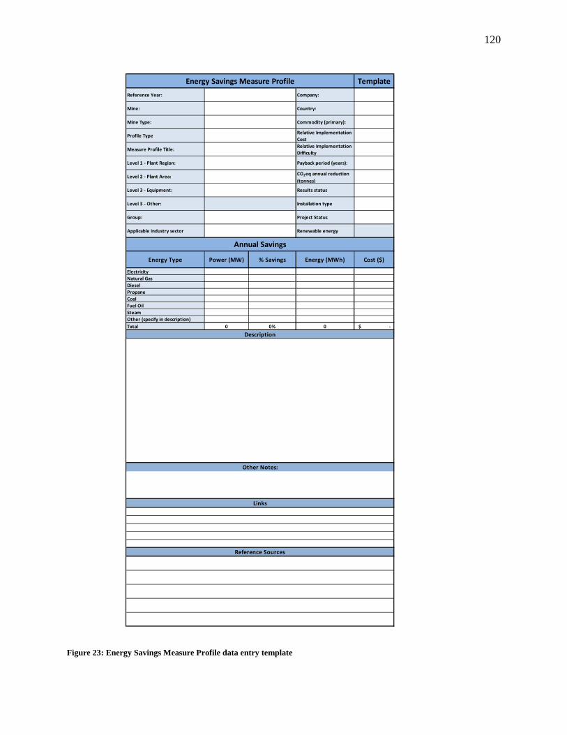
120

Figure 23: Energy Savings Measure Profile data entry template

Template

Reference Year: Company:

Mine: Country:

Mine Type: Commodity (primary):

Profile Type Relative Implementation Cost

Measure Profile Title: Relative Implementation Difficulty

Level 1 - Plant Region: Payback period (years):

Level 2 - Plant Area: CO2eq annual reduction (tonnes)

Level 3 - Equipment: Results status

Level 3 - Other: Installation type

Group: Project Status

Applicable industry sector Renewable energy

Energy Type Power (MW) % Savings Energy (MWh) Cost ($)

ElectricityNatural GasDieselPropaneCoalFuel OilSteamOther (specify in description)Total 0 0% 0 $ -

Description

Energy Savings Measure Profile

Annual Savings

Other Notes:

Links

Reference Sources

121

The information to be compiled in the template can be broken down into 5 sub-sections:

background company information, energy efficiency initiative key data, annual savings,

description, and references.

6.2.4.1 Background company information

The background company information section includes fields for year of project implementation,

company name, mine, country, mine type and commodity. These details provide information

which could be useful for performing an analysis of the data to: i) identify energy efficiency

leaders in the mining industry, ii) construct a timeline of energy efficiency initiatives pertaining

to the mining sector and iii) examine where measures were implemented – underground vs.

surface operations, gold vs. coal mines, etc.

6.2.4.2 Energy efficiency initiative key data

Next, the profile section allows input of key data which will assist users to quickly identify

applicable measures when filtering the information. The data entered in most of these fields is

selected from a drop-down list which allows for the information to be categorized.

The selections for the profile type field include: technology, operating, and maintenance. The

technology type is defined as implementation of new or more efficient equipment, whereas

modifications with respect to operation of equipment or management would be included in the

operating type. The last option, consisting of maintenance concerns change implemented to

maintenance practices.

The fields for Level 1 - Plant Region, Level 2 - Plant Area and Level 3 - Equipment where

included to recognize where the initiatives were implemented at the mine; the various levels

122

allow one to narrow the area down from a high level towards the equipment. This allows

distinguishing between initiatives pertaining to underground versus surface operations as well as

processing, transport or support systems. A measure implemented in comminution, smelting,

refining or leaching for example would be classified as processing whereas the transport heading

would include initiatives relating to mobile equipment and the support category consists of

systems involving heating, cooling, lighting, energy supply, building envelope, compressed air

and steam. An option to select “Other” for the equipment is available if the list does not possess

the specific component but in this case, the user can specify the equipment in question in a

separate field labeled “Level 3 – Other”.

The Group field includes categories which may be assigned to initiatives as follows: Automation,

Conservation, Fuel Switching, Heat Recovery, Improved measurement and monitoring, Internal

policy, Maintenance change, Optimization, Process change, Process control, R&D / new

technology, Renewable energy and Training. Inclusion of this field provides a greater level of

detail with respect to the nature of the energy efficiency initiative.

Relative Implementation Cost and Difficulty were included in the data entry template in order to

provide users with an understanding of the financial commitments and level of expertise required

for implementation of energy efficiency measures. These levels were defined in the Assessment

to Action (A2A) Toolkit’s (Institute for Industrial Productivity 2012) Generic Library. Table 7

provides definitions for each level.

123

Table 7: Relative cost and difficulty level definitions (Institute for Industrial Productivity 2012)

Item Level Definition

Cost

High Implementation cost is very high, and a detailed economic

feasibility analysis (based on a detailed process design) is

required to justify and estimate the cost.

Medium Cost is relatively average, and usually requires a first-order

economic feasibility analysis to justify and estimate the cost.

Low Limited to no cost involved to implement the opportunity.

Generally referred to as "low hanging fruit."

Difficulty

High Replacement of existing, large equipment / process units, or

complex modification to the process, which requires external

expertise to design and implement. Requires a detailed

technical and economic feasibility assessment and detailed

process design prior to implementation.

Medium Replacement of existing, small/medium size equipment /

process units, or relative minor modification to the process,

which can often be design and implemented by in-house

expertise. Retrofit of equipment that require a moderate effort

to implement. Generally requires only a first order technical

and economic feasibility assessment and minor process design

prior to implementation.

Low Process modifications, equipment replacements and retrofits

that are relatively easy to implement. Most often can be

integrated with maintenance activities and include operational

and behavioural changes. A high level economic and technical

feasibility analysis may be required in some instances.

124

Subsequently, fields were included for specification of payback period as well as carbon

emission reductions. The Results status options allows one to distinguish between estimated and

confirmed savings whereas the Installation type explains whether the project consisted of setting

up new equipment, retrofitting existing equipment, replacement of existing equipment or no

installation at all. Whether a project is proposed, in progress or has already been implemented,

may be specified in the Project Status line. The template also allows users to specify which

sector within the mining industry a measure would be applicable to; the options for this field are

the same as those from the Level 1 – Plant Region, which include: underground, open-pit,

process, transport, and support. In instances where renewable energy projects are concerned, the

source can be identified in the Renewable energy field which enables companies to highlight

these types of projects.

6.2.4.3 Annual Savings

The Annual Savings section provides information regarding power (MW), percent, energy

(MWh) and financial savings achieved via the implementation of energy efficiency measures.

The savings are also categorized by the type of energy that is reduced; users can specify

electricity, natural gas, diesel, propane, coal, fuel oil, steam or other source of energy which was

saved by the initiative. In a case where a measure results in lowering multiple energy sources,

savings are entered for each energy type and the sum of these would be shown in the total

savings field.

125

6.2.4.4 Description of energy efficiency initiative

In the next section, an area is provided to supply a description of the energy efficiency measure,

which may include details regarding how energy is saved. A separate field labeled ‘Other Notes’

is included to provide users an opportunity to highlight any other pertinent information which

may have been omitted in the pre-defined fields.

6.2.4.5 References and links for additional information of energy efficiency measure

The last section provides space for users to include hyperlinks to websites as well as reference

sources which could be used to direct other users who wish to obtain additional information to

available resources.

6.2.4.6 Navigation buttons

The buttons on the right-hand side of the template are used navigate between screens as well as

update information in the register. The “Update Database” button’s function is to append the

newly entered information to the existing data and adds the initiative to the index. A user

wishing to enter a new measure would click on the “Enter New Measure” button which opens a

blank template. “Back to Index” and “Back to Menu” buttons allow users to navigate to the

index and menu screens respectively whereas the “Delete Measure” button will permanently

remove a record from the database.

6.2.4.7 Best practice database Index for quick reference

The Mining Energy Efficiency Best Practice database comprises an index which provides a

snapshot of the initiatives included in the register; each row is allocated for individual measures

and the key data is indicated in separate columns.

126

From the index screen, users can filter the data from any of the key fields in order to find

relevant energy efficiency measures. For example, the data can be categorized by company in

order to identify energy efficiency leaders in the mining industry or by payback period to

distinguish initiatives with the quickest return on investment. Alternatively, users may narrow

down the applicable initiatives which may be of relevance to a specific circumstance by

application of a filter to the Equipment or the Applicable industry sector field. In order to gain

perspective with respect to energy and financial savings achieved, figures for each initiative were

included in the index for each energy type. This also provides functionality to isolate projects

which could reduce energy consumption from a specific source. For example, a mine energy

manager wishing to identify measures to reduce diesel consumption could filter the data from the

register to highlight applicable projects to this energy source.

Additional information for any of the initiatives can be obtained from the index by clicking on

the “Tab Number” link in the first column, which will open the Energy Saving Measure Profile

for that specific project. The supplementary data available from this screen includes mine type,

carbon emission savings, renewable energy source, energy efficiency measure description, links

to websites and reference sources.

6.2.4.8 Quality assurance

Dissemination of energy conservation projects can be via journal publications, magazine articles,

corporate sustainability reports, or company websites and newsletters, however these may not all

undergo a peer-review process. Thus, to ensure that the entries in the improved database are

complete and accurate, a checking procedure is used prior to uploading case studies to the

register.

127

The quality checking procedure entails comparing the estimated or reported energy savings

against an estimate of energy use from that demand center to verify that the savings are realistic.

A secondary verification of the energy savings is done by comparison with similar entries.

Currently this procedure is undertaken by an individual that is familiar with energy use in the

mining sector but a future version of the database may include a self-checking procedure. This

may entail that users are required to upload additional information such as the total amount of

energy used annually, but may not necessarily be published due to the sensitive nature of the data

required for checking purposes.

6.2.4.9 Lessons from the database

The goal behind the creation of the Mining Energy Efficiency Best Practice database was to

facilitate dissemination of best practices with respect to energy matters in the mining industry.

To achieve this target, it is essential to populate the register with case studies. The mining

industry energy management database has been made available in the public domain where

mining companies can examine the best practice examples. Mining energy champions may also

contribute to the register by providing case studies; a standardized entry template affords a

quality assurance dimension that is absent in other reporting initiatives.

As the information in the register grows, an analysis may be performed to create a timeline of

energy efficiency initiatives in the mining industry which may reveal trends with respect to focus

areas throughout the years. Alternatively, the Profile Type and Group fields may be utilized to

determine the nature of the implemented measures and assess the mining industry’s behaviour in

energy matters.

128

To date, 107 case studies have been recorded in the Mining Energy Efficiency Best Practice

database, of which annual energy savings for 54 projects have been reported or estimated,

totaling roughly 1.5 million MWh. The entries were from numerous mining companies,

operating in various countries and mining several commodities. The examples dated from 1980

until 2012 and the annual energy savings resulting from initiatives in the mining industry during

these 32 years are illustrated on Figure 24.

Figure 24: Example to illustrate the form of cumulative energy savings curve in mining sector from 1980 to 2012

Although it may appear from Figure 24 that most of the energy savings have been realized

during the most recent years, this may not be accurate since there are gaps in the dataset; the

database contained only one case study from 1980 with the next entries corresponding to 1995

then 2001, but there were entries for every year between 2004 and 2012. Furthermore, the case

studies entered in the database represent a partial account of all energy management initiatives

implemented in the mining industry since the data entry stage is in progress.

0

200,000

400,000

600,000

800,000

1,000,000

1,200,000

1,400,000

1,600,000

1980 1984 1988 1992 1996 2000 2004 2008 2012

Cum

ulat

ive

Savi

ngs (

MW

h/an

num

)

129

Further investigation revealed that, of the 1.5 million MWh energy savings in the mining sector,

most of the savings were realized from technology type initiatives (56%), followed by operating

measures (43%) and very little from maintenance examples (0.2%).

A more detailed analysis of the data was undertaken by examining the annual energy savings

achieved by the various groups of measures. The top 3 groups consisted of heat recovery

examples which provided the most energy savings followed by renewable energy projects then

internal policies. Although renewable energy projects may not result in energy savings, this

category was included in the database since they result in reducing carbon emissions. Figure 25

illustrates the results.

130

Figure 25: Energy savings by group

Additional analysis may ensue as the database matures to examine the energy savings by

commodity, by country, by energy source or by company; depending on the objective of the

investigation any of the fields could be analyzed.

6.2.5 Adopting the improved database

Adoption of the Mining Energy Efficiency Best Practice database with its standardized reporting

mechanism will enhance transparency of the mining industry in energy matters and may help it

maintain its social license to operate.

0

50,000

100,000

150,000

200,000

250,000

300,000

350,000

400,000

450,000An

nual

Sav

ings

(MW

h)

131

Multiple frameworks are currently available to mining companies for promotion of sustainability

initiatives however there seems to be a lack of consistency in these reports which would allow

effective assessment, benchmarking and comparison of energy efficiency measures. The use of a

database to facilitate dissemination of best practices can be effective but the appropriate structure

needs to be implemented so that users can quickly and easily identify applicable measures. The

Australian Government’s Energy Efficiency Significant Opportunities Register comprises

mining industry efforts aimed towards improving energy use. Although this was a good attempt

at improving transparency and dissemination of best practice, an improved database structure

was developed in order to provide a more effective means of identification of relevant

opportunities.

Currently, more than 40 users have downloaded the Mining Energy Efficiency Best Practice

database. Some of these individuals are mining company employees, consultants in the mining

sector, or academics. Increased adoption of the tool may be achieved by targeting its promotion

to these groups. Further enhancements could also be implemented in subsequent versions of the

database to address the needs of various stakeholders which may be achieved through increased

collaboration between users.

132

7 Improved auditing for mines – an example from Garson Mine

An energy audit was conducted at Garson Mine in 2014 as part of a Master’s level project within

the Natural Resources Engineering program at Laurentian University (Mallett 2014). The audit

consisted of gathering data and information that would allow estimating the annual energy

consumption of the various end-uses at the mine.

7.1 Background

Garson Mine is an underground mine located in Sudbury Ontario and is owned and operated by

Vale. Ore is extracted from three orebodies which are accessed either via the Garson Ramp or a

shaft developed to 1,288 meters (Mallett 2014).

A total of 68 pieces of underground equipment including drills, bolters, scissor lifts, and

personnel transportation vehicles, which consume diesel and/or electricity, are used to support

production. Scoop trams and haul trucks transport and dump ore and rock to an ore pass or a rock

pass where the materials are fed to the rail tramming system. These 24 pieces of equipment make

up the underground mobile equipment fleet, all of which consume diesel fuel as an energy

source. The ore is then crushed underground then hoisted to surface via the skip hoist,

consuming electricity for these processes. Personnel and supplies are transported in the cage

hoist from surface to the underground workings, also using electricity. Ventilation fans, powered

by electricity are necessary to supply fresh air to the underground workings. The main

ventilation system at Garson Mine comprises 16 main and booster fans, whereas 54 fans make up

the auxiliary system. The ventilation system also consumes natural gas to heat the mine air

supply during the winter months. Electricity is also consumed by 5 compressors which are used

at the mine to supply compressed air to one of the backfill plants and to pneumatic powered

133

equipment used underground. Process water and inflow water from precipitation is evacuated

from the underground workings with the use of 7 electrically powered pumps located at different

levels underground. The mine also consumes electricity in 2 backfill plants which are used to fill

areas underground where mining activities are complete. Although there are only 10 distinct end-

uses consuming energy at the mine, the number of individual equipment within these categories

can be substantial, thus a detailed energy audit at an underground mine may be challenging.

Furthermore, a mine is a dynamic environment which may pose obstacles to installation of

infrastructure for continuously monitoring the energy use from all equipment.

7.2 Conducting the energy audit

The first step in the energy survey consisted of gathering invoices and metered data to determine

the total annual consumption from each type of energy; these consisted of electricity, natural gas

and diesel. Subsequently, the energy consumption from the various end-uses was measured or

estimated. Table 8 describes the methodology used for estimation of energy consumption for

each end-use.

134

Table 8: Method used to obtain energy consumption from various end-uses at Garson Mine

End-use Data gathering methodology

Ventilation Natural gas consumption was metered. Electricity use was estimated from each individual fan’s rated power and an estimate of the annual operating hours.

Skip hoist Obtained root mean square (RMS) power per cycle from hoist logger and average cycle time to determine the energy use per cycle. Then the number of cycles per month required to hoist the amount of ore produced was calculated and used to estimate the monthly energy consumption.

Cage hoist Obtained root mean square (RMS) power per cycle from hoist logger and average cycle time to determine the energy use per cycle. Then the number of cycles was determined from the cage hoist schedule to estimate the monthly energy use.

Backfill plants Estimated the number of operating hours based on plant capacity and actual fill produced. Then the energy use was estimated with the rated power of the motors in the plants and the estimated operating hours.

Compressors Data obtained from logged meter values

Pumps Data obtained from logged meter values

Surface facilities Estimated 2% of total energy use at the mine

Underground fixed equipment (crusher)

Estimated number of operating hours per year from actual ore production data and tramming capacity. It was assumed that the crusher operating hours corresponded to the tramming time. Annual energy consumed was estimated from the number of operating hours and the crusher’s rated power.

Underground equipment (drills, bolters)

Estimated from the difference between the total electricity use at the mine and the sum of all other end-uses.

Underground mobile equipment

Fuel consumption of each piece of equipment was calculated by the following formula (Hays 1990) as cited by Mallett (2014) :

𝐹𝐶 = 𝐶𝑆𝐹 × 𝑃 × 𝐿𝐹

𝐹𝐷

where 𝐹𝐶 is fuel consumption (L/hr), 𝐶𝑆𝐹 is specific fuel consumption at full power (kg/ kW per hr), 𝑃 is power (kW), 𝐿𝐹 is load factor (%), and 𝐹𝐷 is fuel density (kg/L). The energy consumption for each machine was estimated with the calculated hourly fuel consumption and an estimate of the operating hours.

135

Figure 26 presents a Sankey diagram prepared from the audit data to illustrate the energy

consumption allocated to the various end-uses.

Figure 26: Energy flows at Garson Mine

Figure 26 shows that ventilation, and underground equipment were the main electricity

consuming activities. However, the electricity consumption from the auxiliary mine ventilation

system seemed low whereas the use from drills and bolters appeared high.

136

7.3 Reconciling the data

A review of the equipment inventory, power rating and load factors for these demand centers

revealed that the electricity use from underground equipment may have been overestimated

whereas the auxiliary ventilation consumption was underestimated. For example the weighted

average rated power from all auxiliary fans in the inventory corresponded to roughly 50 kW and

it is assumed that these had a 97.5% load factor, which corresponded to the load factor attributed

to the main fans in the study. Conversely, the average rated power of the hydraulic power pack

for the underground equipment (bolters and drills) was 75 kW but the average load factor for

electricity consuming activities for these units corresponds to roughly 25% (Hauta 2015).

Although the average rated power for the drills and bolters was higher than that of the auxiliary

fans, the load factor and the number of equipment was lower. There were more than 50 auxiliary

fans in the inventory whereas there was a total of 15 drills and bolters. Thus it is anticipated that

the electricity consumption from the auxiliary ventilation fans would be greater than that of the

drills and bolters. As such, the electricity consumption of the drills and bolters was estimated

from the rated power and the average load factor values. It should be noted that the rated power

of the hydraulic power packs for the drills and bolters was obtained from manufacturer’s

technical specification sheets and catalogues (Boart Longyear 2014, Cubex Ltd. 2010a, Cubex

Ltd. 2010b, Cubex Ltd. nd., Sandvik Mining and Construction 2007, Tamrock 1995, Tamrock

2000). In some instances, model numbers were not included in the inventory thus the rated

power value used in the estimate corresponded to the maximum value listed for the equipment

series. Further, the value for the drills and bolters from the original audit was 242% greater than

that from an estimate with a load factor of 100%.

137

A review of the auxiliary fan inventory revealed that 42 of the 54 auxiliary fans were excluded

from the original audit, thus this supported the hypothesis that the consumption from this

demand center may have been underestimated. The other remaining unknown value from the

audit corresponded to the electricity consumption of the surface facilities, which was allocated an

arbitrary value of 2% of total energy consumption in the original audit. As such an attempt was

made to balance the electricity use at the mine. The electricity consumption of the auxiliary mine

ventilation system was estimated using the rated power and a 97.5% load factor for all the units

from the fan inventory, which left 6% of total electricity for the surface facilities. This value

seemed high and since there were some fans from the inventory with unknown locations it was

decided to keep the electricity use from the surface facilities at 2% of total and allocate the

balance to the auxiliary mine ventilation system to account for fans with unknown locations.

Installation of electricity meters to quantify the surface electricity consumption as well as

updating the fan inventory would either confirm these revised values or provide more accurate

estimates. Subsequently a revised Sankey diagram was prepared from the revised energy

consumption values for Garson Mine which is presented in Figure 27.

138

Figure 27: Revised Sankey diagram for energy flows at Garson Mine

It can be seen from Figure 27 that the end-uses consuming the most energy, thus those that future

work should focus on were: ventilation, and underground mobile equipment.

The Garson Mine energy audit illustrated a snapshot of energy use at this site with many

estimated values, but provides a basis for further refinement. Table 8 shows that the natural gas

consumption and the electricity use from the pumps and compressors were the only values

obtained from metered data comprising 23% of energy use thus estimates were used to allocate

139

77% of total energy used at his mine. The preliminary audit permitted the identification of

information gaps as presented in the Top-down energy audit method (Rosenqvist, Thollander et

al. 2012). Thus re-iteration of the Garson Mine energy audit with adoption of an improved

methodology may enhance confidence in the audit values.

7.4 An improved energy audit methodology for Garson Mine

The following recommendations are suggested and it is anticipated that adoption of these

measures could lead to an improved energy management methodology for Garson Mine.

• Install meters on main ventilation fans (16 meters required)

• Install meters to obtain electricity use from skip and cage hoists (2 meters required)

• Install meters at the plant level for backfill plants (2 meters required)

• Install meter to gather electricity use from underground fixed equipment (crusher) (1

meter required)

• Install meters for surface facilities (4 meters required)

• Include blasting as an additional end-use

• Obtain diesel consumption for underground mobile equipment and underground

equipment (drills, bolters…) from engine management systems

• Obtain ventilation survey data and accurate fan inventory from ventilation group to

estimate electricity use from auxiliary ventilation system.

• Gather and analyze data for a 12 month period.

• Collect data for factors that influence energy consumption as presented in Table 9

140

Table 9 also indicates the expected diurnal and seasonal variability as well as potential

demand side management (DSM) measures to reduce energy use for each demand center.

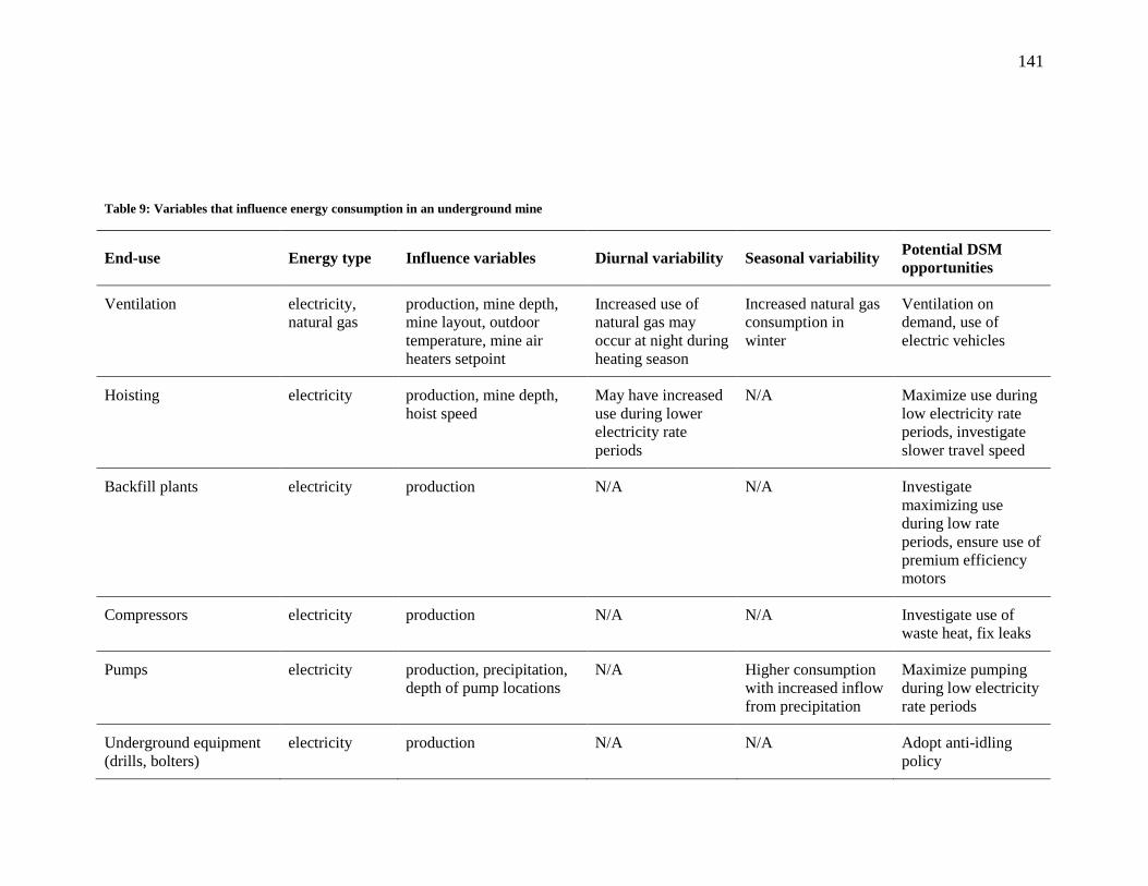
141

Table 9: Variables that influence energy consumption in an underground mine

End-use Energy type Influence variables Diurnal variability Seasonal variability Potential DSM opportunities

Ventilation electricity, natural gas

production, mine depth, mine layout, outdoor temperature, mine air heaters setpoint

Increased use of natural gas may occur at night during heating season

Increased natural gas consumption in winter

Ventilation on demand, use of electric vehicles

Hoisting electricity production, mine depth, hoist speed

May have increased use during lower electricity rate periods

N/A Maximize use during low electricity rate periods, investigate slower travel speed

Backfill plants electricity production N/A N/A Investigate maximizing use during low rate periods, ensure use of premium efficiency motors

Compressors electricity production N/A N/A Investigate use of waste heat, fix leaks

Pumps electricity production, precipitation, depth of pump locations

N/A Higher consumption with increased inflow from precipitation

Maximize pumping during low electricity rate periods

Underground equipment (drills, bolters)

electricity production N/A N/A Adopt anti-idling policy

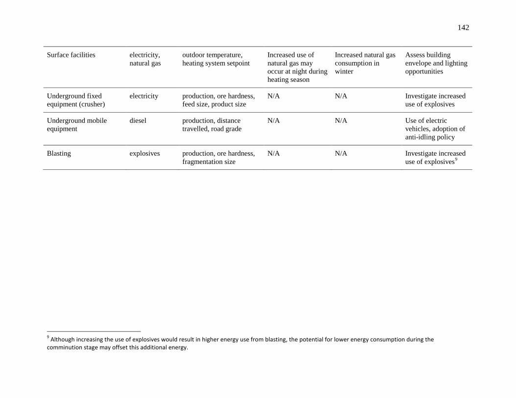
142

Surface facilities electricity, natural gas

outdoor temperature, heating system setpoint

Increased use of natural gas may occur at night during heating season

Increased natural gas consumption in winter

Assess building envelope and lighting opportunities

Underground fixed equipment (crusher)

electricity production, ore hardness, feed size, product size

N/A N/A Investigate increased use of explosives

Underground mobile equipment

diesel production, distance travelled, road grade

N/A N/A Use of electric vehicles, adoption of anti-idling policy

Blasting explosives production, ore hardness, fragmentation size

N/A N/A Investigate increased use of explosives9

9 Although increasing the use of explosives would result in higher energy use from blasting, the potential for lower energy consumption during the comminution stage may offset this additional energy.

143

The installation of 25 additional electricity meters at Garson Mine, to monitor the electricity use

from fixed equipment, would reduce the uncertainty of electricity use within 6 of the studied

end-uses. Thus if all the electricity consumed by fixed equipment is metered and ventilation

survey data is used to estimate the auxiliary ventilation consumption, the remaining balance can

be allocated to the mobile equipment. Furthermore, use of vehicle engine management systems

to determine diesel consumption from the underground mobile equipment and production

support equipment would provide further confidence in the audit values. Thus with these

proposed refinements to the Garson Mine audit, the proportion of metered data would increase

from 23% to 78% of total energy at the mine based on the allocated energy values from the

preliminary audit.

Ideally, all equipment should be metered to assess energy use but in an underground mine this

may not be practical. An underground mine is a dynamic environment with development

occurring in several areas, where installation of meters on auxiliary fans for example would have

to be relocated with the fans as areas are developed. Thus, it was suggested to estimate the

energy consumed from this end-use from ventilation survey data. In Ontario testing is required

on a weekly basis to determine the air volume flowrate where diesel equipment is used as per

Regulation 854 Section 183.2 (Workplace Safety North 2011). Therefore combining knowledge

of the fan model and blade setting with the measured flowrate values can be used to determine

the fan operating pressure from the manufacturer’s fan curves. This information can also be used

to determine the fan efficiency, all of which could be used to calculate the fan electricity

consumption as shown in (2) (McPherson 1993).

144

𝑾 = 𝑷×𝑸𝜼𝒇𝒂𝒏×𝜼𝒎𝒐𝒕𝒐𝒓

(2)

where 𝑊 is the power (kW), 𝑃 is the fan pressure (kPa), 𝑄 is the airflow rate (m3

Implementation of the aforementioned recommendations for improving the Garson Mine audit

would leave only the electricity consumed by the underground equipment (drills, bolters…) as

fully estimated values. In the preliminary audit the energy use from these was allocated based on

the difference between the sum of all other electricity and the total consumed at the mine. A

value of 2% was allocated to the surface facilities and the remaining balance to the underground

equipment. Monitoring the electricity use from equipment within the underground equipment

category was not suggested as an improvement to the audit since it may be challenging because

these are mobile units. Some of the 68 pieces of equipment consume both diesel and electricity;

diesel is used for mobility whereas the electricity is used for powering the equipment’s specific

application. For example, electricity can be used to power the drilling mechanism on a drill. Thus

installation of electricity meters on mobile units may not be practical. All of the 68 pieces of

equipment in the underground equipment category use diesel for mobility regardless if these

/s), 𝜂𝑓𝑎𝑛 is the

fan efficiency, and 𝜂𝑚𝑜𝑡𝑜𝑟 is the motor efficiency. An estimate of the motor efficiency and fan

operating hours would be required to determine the energy use from each fan. Although this

would only provide the energy use corresponding to the period where the ventilation survey was

conducted, it would be better than using the rated power with an assumed fan efficiency.

Furthermore, the location of some of the auxiliary fans listed in the inventory was labeled as

“unknown” during the preliminary audit thus it is possible that the electricity consumption

allocated to the ventilation system may be incorrect. Therefore coordination with the ventilation

team to gather an updated fan inventory list would eliminate some of the uncertainty.

145

consume electricity for additional purposes. Thus diesel consumption may be obtained from

engine management systems, and the electricity use would be the only estimated energy use from

this category.

Gathering data for the variables listed in Table 9 could permit an assessment of diurnal or

seasonal variability in energy use, as well as establishment of benchmarks from the individual

end-uses. This may facilitate the analysis stage of the audit and the identification of potential

energy conservation measures. Subsequently, these variables could be used in a Level 3 energy

audit, whereby potential savings from energy conservation measures may be quantified with the

use of models.

The preliminary Garson Mine energy audit consisted of a bottom-up / energy balance audit

method, and corresponded to a level between Level 1 and Level 2 as defined by ASHRAE

standards. The Garson study was more in-depth than a walk through audit since data was

gathered and energy use was allocated to the various end-uses. However it lacked a thorough

analysis step to identify potential energy conservation measures that would be included in a

Level 2 audit.

Review of the Garson Mine audit provided a starting point for assessing energy use in an

underground mine and provided the basis for development of an improved energy audit

methodology which may be adopted at other mine sites. The proposed method can be

generalized as follows:

Conduct a Level 1 or a walk-through audit consisting of reviewing historical energy billing data

for all energy types to provide an overview of the amount of energy consumed at a site. Then a

146

site visit ensues to identify obvious energy conservation measures. For an underground mine

these could include identification of:

• leaks (for example from compressed air, ventilation, or pumping systems)

• idling equipment (such as conveyors running empty, or idling vehicles)

• sources and sinks for waste heat

• low equipment utilization (such as equipment running but not fully loaded).

Subsequently, conduct a preliminary audit by gathering all available metered data and estimating

energy consumption for the remaining end-uses. The purpose of this audit is to identify

information gaps which may be addressed with future iterations of the audit, providing a basis

for continuous improvement. It is suggested to install meters to monitor energy use from all fixed

equipment and whenever possible on mobile equipment; the greater proportion of energy that is

metered improves the confidence in the audit.

Subsequently, a level 2 energy audit may be conducted with sufficient confidence to identify

potential energy conservation measures. If installation of meters is not feasible due to physical or

budgetary constraints, it is recommended to use the energy balance audit method as described in

Pawlik et al (2002). Inclusion of a utilization factor, equipment efficiency, motor load factor, and

a diversity factor in addition to the equipment rated power and an estimate of the annual

operating hours may result in a more accurate estimate of energy use. Furthermore, this method

provided guidance to adjust estimated values when the sum of individual equipment and the total

consumption at a site did not balance.

Use of the CIPEC Energy Savings Toolbox (Natural Resources Canada 2009) is recommended

for the data analysis step of the audit. The key to identification of potential energy savings

147

measures begins with an understanding of how, when and why energy is used at a facility. The

guidance and tools included could be adapted to suit the mining industry which may provide a

systematic method for data analysis and identification of energy conservation measures, which

was employed by New Afton Mine during implementation of ISO 50001 (Clean Energy

Ministerial 2014).

Where reduced uncertainty in the energy savings from the proposed measures is required, a

Level 3 audit may ensue to model the specific system or equipment. However, these models

should also consider the impact of the proposed measures on downstream processes. For

example, reducing the energy used in blasting may increase the energy used in the comminution

stage of the process, thus an integrated approach is recommended to ensure that the overall

energy use at the site is minimized. Figure 28 illustrates an overview of the proposed energy

management methodology with a continuous improvement approach.

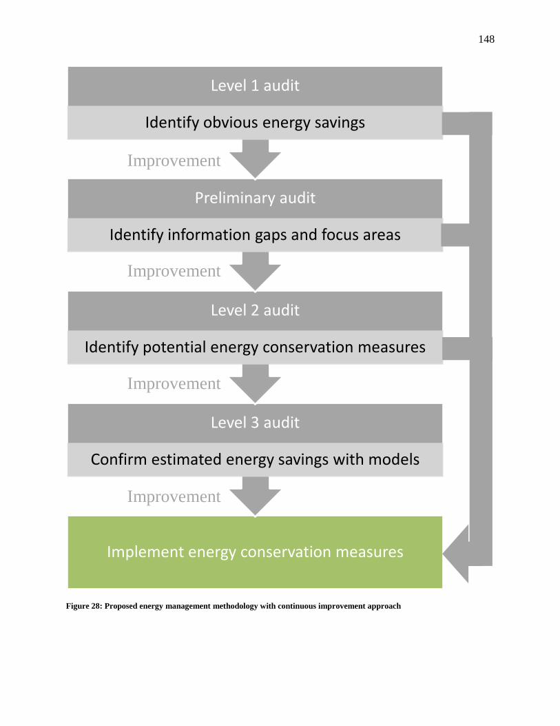
148

Figure 28: Proposed energy management methodology with continuous improvement approach

Implement energy conservation measures

Level 3 audit

Confirm estimated energy savings with models

Level 2 audit

Identify potential energy conservation measures

Preliminary audit

Identify information gaps and focus areas

Level 1 audit

Identify obvious energy savings

Improvement

Improvement

Improvement

Improvement

149

8 Improved interpretation of energy consumption data - Energy

management pertaining to auxiliary mine ventilation systems

8.1 Introduction

As can be appreciated from the previous Chapter, ventilation can account for a significant

portion of the electricity consumption in underground mines. As such, any gains that can be

made to improve energy use for ventilation of the sub-surface can have an impact on the

facility’s overall energy costs.

Research and/or experience has identified that savings could be obtained in ventilation systems

from measures including, but not limited to, ventilation on demand (VOD) (Bartsch, Laine et al.

2010) or fan drive frequency control (Wang, Chen et al. 2010). Potential savings for VOD

implementation estimated by Bartsch et al. corresponded to 52.8% and 36.5% for electricity and

propane respectively. Alternatively, innovative materials with lower friction factors could also

have the potential to provide energy savings, ranging from 56% to 71% depending on the

materials compared, as exemplified in Tardiff et al. (2010) however their overall economic value

needs further assessment and has been examined within this Chapter.

A series of ventilation surveys were conducted at Mining Technologies International Inc.

(MTI)’s underground research and demonstration site, located in Lively, Sudbury, Ontario,

Canada, to: i) quantify the Atkinson friction factor of the polyethylene auxiliary ventilation duct,

and ii) quantify the possible energy savings from use of this material, compared to some of the

more conventional products used in the mining sector, such as steel and layflat ducts.

150

An auxiliary mine ventilation model was developed to assess energy and life cycle costs and

hypothetical case studies were examined to compare the economics of various systems.

8.2 Ventilation survey methodology

The survey was conducted by measuring the static pressure, at various fan speeds, at two duct

stations, separated by a distance of 125 meters. Figure 29 shows the layout of the facility and the

locations where measurements were taken. Q1 corresponds to the surface fan location where air

velocity measurements were taken, whereas P1 and P2 are the static pressure reading locations

for the plastic duct. The inset in the figure shows a schematic of the elevation view between the

pressure measurement stations.

151

Figure 29: MTI Mine layout and ventilation survey measurement locations (inset illustrates a side view of the pressure measurement locations)

152

The use of two barometers and two manometers allowed for simultaneous pressure observations

at both locations. Measurements using the barometers followed the ‘leapfrog’ procedure

(McPherson 1993) except that since there were only two measurement locations the barometers

remained at the same locations.

Static pressure observations were also recorded simultaneously at both locations with the use of

two manometers with the high port connected to a plastic tube inserted in the side of the duct and

the other gauge port open to atmosphere inside the drift. Two trials were conducted for each of

the 5 fan speeds tested, with each trial consisting of an average of 5 pressure values.

The elevation difference between the measurement locations needed to be considered for

determination of the pressure drop when using the barometer values, whereas the elevation

difference was cancelled when using the manometer readings, illustrated by the inset in Figure

29. Points A and B indicated the location of the pressure differential between the duct and the

drift measured by the manometer at station P1 whereas C and D represented the corresponding

measurement points at P2. The elevation difference between points A and C in the duct was the

same as the elevation difference between B and D in the drift, therefore the difference between

the simultaneous manometer readings at P1 and P2 would be equivalent to those taken on a

horizontal level, providing that the drift resistance is negligible compared to the duct resistance

which is often the case according to Duckworth and Lowndes (2003).

For each fan speed, the duct air velocity was measured with the use of a hot wire anemometer.

Measuring positions were determined for an 8 point traverse following the log-linear traverse

method for a circular duct (McPherson 1993). Three measurement values, all within 5% of one

another were recorded and averaged for each measuring position inside the duct. However, the

153

hot wire anemometer could only reach up to the center of the duct thus it was not possible to

obtain values at all of the measuring points. Therefore only half of the duct velocity profile could

be measured and it was assumed that both halves were symmetrical. The four velocity values

were then averaged to determine the air velocity inside the duct at each fan speed. Table 10

shows the measuring positions of the traverse from the side of the 1.2 m diameter duct but only

the first four points were measured.

Table 10: Velocity measurement positions

Point Fraction of diameter

(McPherson 1993)

Distance from side

of duct (m)

1 0.021 0.026

2 0.117 0.143

3 0.184 0.224

4 0.345 0.421

5 0.655 0.798

6 0.816 0.995

7 0.883 1.076

8 0.978 1.192

Subsequently air velocity measurements were taken for a complete 8 point log-linear traverse as

per the locations in Table 10 which revealed that the velocity profile was not symmetric as is

illustrated in Figure 30, thus the original values were discarded and the survey was repeated. It

should be noted that the values recorded during the first survey with only 4 points corresponded

154

to those from ~0.8 to 1.2 m across the duct, thus the average air velocity values from these trials

was overestimated.

Figure 30: Air velocity values for 8 point log-linear traverse at various fan speeds

It was suspected that the silencer located prior to the measurement location was the cause of the

asymmetry in the velocity profile, thus a new air velocity measurement location was chosen.

Furthermore, one of the duct segments at the beginning of the system was damaged between the

time of the original and revised surveys therefore a new location was also selected for the P1

pressure measurement location from Figure 29. This new location, which also corresponded to

the new air velocity measurement station, was chosen to be at least 10 duct diameters past the

0

5

10

15

20

25

30

0 0.2 0.4 0.6 0.8 1 1.2 1.4

Mea

sure

d av

erag

e ai

r vel

ocity

(m/s)

Distance across duct (m)

60 Hz55 Hz50 Hz45 Hz40 Hz35 Hz30 Hz25 Hz20 Hz

155

first bend in the system. A distance of 107 m separated the pressure measurement locations for

this survey.

An 8 point log-linear duct traverse methodology was used in the new survey however, since

measurements were taken from both sides of the duct, both values in the center were recorded

from each side of the duct for verification purposes. The duplicate values were averaged and

treated as one value with the other data to calculate the average air velocity in the duct. Figure 31

illustrates the measurement locations inside the duct with the numbers corresponding to the

sequence of the measurement whereas Figure 32 shows the velocity profile of the new survey.

Figure 31: Measurement location and sequence of 8 point log-linear traverse along the duct

156

Figure 32: 8 point velocity profile for new survey

Use of the duct diameter to calculate the cross-sectional area allowed determination of the

volumetric flowrates from the velocity values. Psychrometric measurements (dry bulb and wet

bulb temperatures) were also taken with a whirling hygrometer to determine the air density in the

drift between the pressure measurement points during the survey.

8.3 Determination of friction factor

8.3.1 Friction factor calculations

The first step consisted of determination of the frictional pressure drop between both pressure

measurement locations (P1 and P2) for each fan speed. This was achieved by determining the

difference between both manometer readings because the use of these eliminated the need to

0

5

10

15

20

25

0.0 0.2 0.4 0.6 0.8 1.0 1.2 1.4

Velo

city

(m/s

)

Distance across duct (m)

60 Hz

50 Hz

40 Hz

30 Hz

20 Hz

157

correct for the difference in elevation between the measurement stations. The difference between

the barometer values with correction for the elevation difference was used to verify the

manometer readings.

Air density is a variable that was used in several formulas for determining the Atkinson friction

factor. Measurements of the atmospheric pressure, the dry bulb and wet bulb temperatures were

used to calculate the value of the air density, using equations 14.6, 14.10, 14.4, 14.32 and 14.14

from McPherson (1993). Then the general gas law was used to calculate the specific volume of

the air/vapor mixture and the reciprocal of this value provided the air/vapor mixture density.

The following step consisted of calculation of the flowrate (𝑄) from velocity measurements (𝑢)

and the dimension of the duct area (𝐴) using:

𝑸 = 𝒖𝑨 (3)

The next step consisted of calculation of the total resistance (𝑅) in the system between the two

measurement locations. This was achieved with (4) , where 𝑃 corresponded to the pressure

difference from the manometer readings between measurement locations and 𝑄 was the flowrate.

𝑹 = 𝑷𝑸𝟐

(4)

The total resistance (𝑅) between P1 and P2 comprised i) frictional resistance in the duct, ii)

frictional resistance in the drift, iii) equivalent Atkinson resistance from shock losses in the duct,

and iv) equivalent Atkinson resistance from shock losses in the drift, all of which are in series:

𝑹 = 𝑹𝒇𝒓.𝒅𝒖𝒄𝒕 + 𝑹𝒇𝒓.𝒅𝒓𝒊𝒇𝒕 + 𝑹𝒔𝒉𝒐𝒄𝒌 𝒅𝒖𝒄𝒕 + 𝑹𝒔𝒉𝒐𝒄𝒌 𝒅𝒓𝒊𝒇𝒕 (5)

Calculation of the shock losses due to the bends in the duct and the drift were carried out as

follows:

158

1. The shock loss factor (𝑋90) for a right angled bend of circular cross section corresponding

to 0.13 was determined from Figure 5.A.1 in McPherson (1993).

2. A correction factor (𝑘) for bends of angles other than 90° corresponding to 0.40 for the

28° bend was determined from Figure 5.A.3 in McPherson (1993).

3. The shock loss factor (𝑋𝜃) for each bend at angle 𝜃 was determined using:

𝑿𝜽 = 𝑿𝟗𝟎 ∗ 𝒌 (6)

4. The equivalent Atkinson resistance (𝑅𝑠ℎ𝑜𝑐𝑘) was determined from (7), where 𝜌 was the

air density and 𝐴 referred to the cross-sectional area of the airway.

𝑹𝒔𝒉𝒐𝒄𝒌 = 𝝆𝑿𝜽𝟐𝑨𝟐

(7)

5. Steps 1-4 were repeated for all bends in the duct as well as the drift. The total equivalent

Atkinson shock resistances for the duct and the drift were determined by summing the

respective values.

The frictional resistance in the drift (𝑅𝑓𝑟.𝑑𝑟𝑖𝑓𝑡) was calculated with the dimensions of the airway,

and the friction factor (k) for an ‘unlined, typical conditions, no major irregularities’ airway

value corresponding to 0.012 kg/m3 (8), determined from McPherson (1993), and applied to ,

where 𝐿 was the length between measurement locations, 𝑝𝑒𝑟 was the perimeter length of the

drift, and 𝐴 was the cross-sectional area of the drift.

𝑹𝒇𝒓.𝒅𝒓𝒊𝒇𝒕 = 𝒌∗𝑳∗𝒑𝒆𝒓𝑨𝟑

(8)

Then, rearranging (5) allowed determination of the frictional resistance in the duct (𝑅𝑓𝑟.𝑑𝑢𝑐𝑡).

Table 11 shows the average resistance values from all of the trials and the proportion of total

resistance from each of the components.

159

Table 11: Resistance of ventilation system components

Resistance (Ns2/m8 % of total

resistance

)

𝑅 0.5435

𝑅𝑓𝑟.𝑑𝑟𝑖𝑓𝑡 0.0012 0.23

𝑅𝑠ℎ𝑜𝑐𝑘 𝑑𝑟𝑖𝑓𝑡 0.00004 0.01

𝑅𝑠ℎ𝑜𝑐𝑘 𝑑𝑢𝑐𝑡 0.0229 4.22

𝑅𝑓𝑟.𝑑𝑢𝑐𝑡 0.5193 95.54

Subsequently, the Atkinson friction factor (𝑘) for the duct could be determined from (9), where 𝐿

was the length between measurement locations, 𝑝𝑒𝑟 was the perimeter of the duct, and 𝐴 was the

cross-sectional area of the duct.

𝒌 = 𝑹𝒇𝒓.𝒅𝒖𝒄𝒕∗𝑨𝟑

𝑳∗𝒑𝒆𝒓 (9)

The friction factor values determined using the experimental data were then corrected to standard

air density using (10), thus allowing comparison to published values, where 𝑘 corresponded to

the experimental friction factor, and 𝜌 corresponded to the air density observed during the trials.

𝒌𝟏.𝟐 = 𝒌 �𝟏.𝟐𝝆� (10)

8.3.2 Error analysis

To assess the uncertainty or error associated with each of the calculated friction factor values, a

Monte Carlo simulation following the methodology outlined in Xiao and Vien (2003) and

Sonnemann et al (2003) was used with the omission of the sensitivity analysis. However, the

160

former study conducted the Monte Carlo simulation with 1,500 trials and the latter reference

indicated that at least 10,000 trials were required to establish sufficient confidence, but this may

not always be the case as the number of simulations is dependent on the number of variables in

the model according to (11) (Harr 1987)

𝑵 = �𝒉𝜶

𝟐�𝟐

𝟒𝜺𝟐�𝒎

(11)

where ℎ𝛼2�corresponded to the confidence coefficient for a normal distribution, 𝜀 corresponded

to the maximum allowable estimate error, and 𝑚 corresponded to the number of variables.

The probability density function was determined for each variable. It was assumed that all

variables followed a normal distribution, but a Beta distribution resembling the normal

distribution was used to limit the range of possible values which prevented the occurence of

unrealistic extreme values in the model.

A Monte Carlo simulation was then run to determine the uncertainty associated with the

calculated friction factor values by varying: both manometer pressure values, the air velocity, the

dry bulb and wet bulb temperatures and the barometric pressure values. The Monte Carlo

simulation was carried out for each of the 10 sets of data, from which the mean friction factor

and standard deviation were calculated within 10% of the value at a 95.45% confidence level.

Table 12 provides a summary of the results.

161

Table 12: Summary of friction factor simulation results

Fan

frequency

(Hz)

Pressure

drop (Pa)

Flowrate

(m3

Friction

factor 𝑘1.2

(kg/m

/s) 3

Standard

deviation

)

Lower

limit

Upper

limit

95.45% confidence

20 56.2 9.86 0.0022 7.6E-5 0.0019 0.0024

20 69.0 9.86 0.0027 8.6E-5 0.0024 0.0030

30 127.5 15.01 0.0021 6.5E-5 0.0019 0.0023

30 121.8 15.01 0.0020 6.3E-5 0.0018 0.0022

40 181.1 20.33 0.0016 5.1E-5 0.0014 0.0018

40 213.7 20.33 0.0019 5.8E-5 0.0017 0.0021

50 318.7 24.91 0.0019 5.7E-5 0.0017 0.0021

50 336.0 24.91 0.0020 5.9E-5 0.0018 0.0022

60 316.9 25.09 0.0019 5.6E-5 0.0017 0.0020

60 332.6 25.09 0.0020 5.8E-5 0.0018 0.0021

Average 0.0020 6.3E-5 0.0018 0.0022

8.3.3 Other quoted friction factor values for low friction ducts

The friction factor value determined during the ventilation survey at MTI’s Test Mine was

subsequently compared to other values reported for plastic ducts presented in Table 13.

162

Table 13: Atknison friction factors reported for plastic ducts

Friction factor (kg/m3 Duct diameter (m) ) Reference

0.0004 1.05 (Tardif, Paquet et al. 2010)

0.0006 N/A (G+ Industrial Plastics Inc. 2014)

0.0009 N/A (G+ Industrial Plastics Inc. nd.)

0.0009 N/A (Mecanicad nd.)

0.0021 1.2 (Ventilation engineer 2015)10

0.0023

1.2 (Ventilation engineer 2015)

0.0028 0.7 (Ventilation engineer 2015)

0.0025 0.5 (Ventilation engineer 2015)

The lowest friction factor value presented in Table 13 was sourced from a publication which was

co-authored by a representative of one of the plastic duct manufacturers. The reported friction

factor value was evaluated from an auxiliary ventilation system installed at the Casa Berardi

Mine, located in Quebec, Canada. The next highest values ranging from 0.0006 to 0.0009 were

from plastic duct manufacturers’ sources whereas the higher values were from ventilation

surveys conducted in actual auxiliary mine ventilation systems. It is interesting to note that these

higher values correspond well with the value obtained from the MTI ventilation survey.

8.3.4 Surface roughness

Subsequently, a sample of the material used to fabricate the plastic ducts tested at MTI’s Test

Mine was obtained from the manufacturer. The purpose of this was to determine the asperity

10 These data were obtained via personal communication with the Principal Engineer – Ventilation at a mine but due to confidentiality reasons the name of this source cannot be disclosed.

163

height, which would provide an alternative method to calculate the material friction factor and

assess the validity of the ventilation survey results as well as the other reported values.

The sample was examined using a reflected light microscope equipped with a QImaging

MicroPublisher™ 5.0 camera. The asperity height was determined by focusing the microscope

on the duct material surface, then focus on the asperity peaks was achieved by adjustment along

the optical axis, whereby the difference between these positions, measured with a micrometer,

corresponded to a height of 5µm ±3µm. The error range was determined by taking several

measurements of the distance between the material surface and the asperity peak planes. Figure

33 and Figure 34 show samples of the images focused on the material surface and the asperity

peaks respectively.

164

Figure 33: Sample image with microscope focus on the material surface plane

Figure 34: Sample image with microscope focus on asperity peaks plane

50µm

50µm

165

It can be observed from Figure 33 and Figure 34 that there were scratches in the duct material

sample as well as a texture, which was assumed to be attributed to a coating applied to the

surface. It was also determined that the major factor contributing to the roughness was the

coating since the sample observed in Figure 33 did not show any roughness on the material

surface.

Determination of the friction factor from the surface roughness, measured as asperity height,

consisted of calculation of the Reynolds number to determine the flow regime from the testing

conducted at the MTI test mine. The values ranged from 7.1E+5 to 1.8E+6 with the average

corresponding to 1.4E+6, therefore it was determined that the flow was turbulent.

Subsequently, the relationship between the Atkinson friction factor and the asperity height for

turbulent flow was examined using the Von Kármán equation (Duckworth, Loomis et al. 2012,

McPherson 1993):

𝒇 = 𝟐𝒌𝝆

= 𝟏

𝟒�𝟐 𝐥𝐨𝐠𝟏𝟎�𝒅𝒆�+𝟏.𝟏𝟒�

𝟐 (12)

where: 𝑓 was the Chezy-Darcy coefficient of friction

𝑘 was the Atkinson friction factor (kg/m3

𝜌 was the air density (kg/m

)

3

𝑑 was the hydraulic mean diameter (mm)

)

𝑒 was the asperity height (mm)

Using the range of asperity height of 5µm ±3µm, determined from the microscopic material

surface observations, the Atkinson friction factor for a 1.2 m diameter duct and an air density of

1.2 kg/m3 Table 14 was calculated. The results are presented in .

166

Table 14: Atkinson friction factor values calculated from asperity height measurements

Asperity height (µm) Atkinson friction factor (kg/m3

2

)

0.0009

5 0.0011

8 0.0011

It can be seen from Table 14 that the Atkinson friction factor values that were calculated from

the asperity height measurements were lower than those obtained during the ventilation survey in

Table 12 as well as those from the ventilation surveys in Table 13, but were close to those

reported from the manufacturer’s sources.

8.3.5 Friction factor of hydraulically smooth pipes

The discrepancies between the reported Atkinson friction factor values for plastic ducts as well

as those obtained from the microscopic analysis prompted an investigation to determine a value

that could be used to characterize a plastic duct. The Atkinson friction factor values for a smooth

tube were determined for various Reynolds numbers. Figure 35 shows a Moody chart where the

dashed lines labeled 1 and 6 correspond to the limits that determine turbulent flow, the dashed

lines labeled 2 and 3 correspond to the range of Reynolds number values from the ventilation

survey at MTI, and the dashed lines labeled 4 and 5 represent the values corresponding to a 4 m/s

air velocity in a 5x5m drift supplied by a 1.2 m and 0.6 m diameter duct respectively. This

corresponds to the recommended maximum air velocity value in a working face as reported in

McPherson (1993). The smooth tube line examined corresponded to that having an 𝜀𝐷

value of

0.000001 on Figure 35.

167

Figure 35: Moody chart (Perry, Green et al. 1997)

1 2 3 4 5 6

168

The Atkinson friction factor values at each Reynolds number (NRe

Figure 35

) were calculated by using the

corresponding friction factors read from , a value of 1.2 kg/m3

for air density, and (12),

the Von Kármán equation (Duckworth, Loomis et al. 2012, McPherson 1993).

Table 15: Friction factors for a smooth pipe at various Reynolds numbers

Defined point on Moody chart N f Re k (kg/m3

Minimum N

)

Re 4.0E+3 for turbulent flow 0.0095 0.0057

Minimum NRe 7.1E+5 from MTI survey 0.003 0.0018

Maximum NRe 1.8E+6 from MTI survey 0.0026 0.0016

NRe 7.2E+6 in a 1.2 m duct supplying a 5x5m drift with maximum velocity of 4 m/s at working face

0.0021 0.0013

NRe 1.4E+7 in a 0.6 m duct supplying a 5x5m drift with maximum velocity of 4 m/s at working face

0.0018 0.0011

Maximum NRe 1.0E+8 on Moody chart 0.0015 0.0009

The values from Table 15 show that the Atkinson friction factor for a smooth pipe ranges from

0.0009 to 0.0057 kg/m3

Table 13

depending on the flow as described by the Reynolds number. Thus the

Atkinson friction factor values presented herein are within the accepted range for a smooth pipe

with the exception of two of the values presented in which indicated that these were

smoother than a smooth pipe and so must be disregarded.

169

8.4 Techno-economic assessment of ventilation systems with various duct friction

factors

The interactions between the variables in an auxiliary mine ventilation system can be complex;

changing one value can alter multiple parameters. An interaction matrix, illustrated in Figure 36,

was established to illustrate the dependencies between the variables in a mine ventilation system.

The shaded boxes represent the variables and the links between them are in the boxes located at

the intersection of the variables. For example, the effect of the fan on the flowrate is located in

the upper right hand corner; changing the fan or the speed leads to a new operating point and

hence a new pressure and flowrate. The effect of flowrate on money can be found in the third

box from the left in the bottom row, which indicates that a change in flowrate leads to a change

in power that is translated to a change in energy cost.

170

Figure 36: Interaction matrix of mine ventilation system variables

Although a lower friction factor could result in lower energy consumption it is equally important

to consider the capital costs for a given system to assess the financial viability of a project. A

model was derived to conduct a techno-economic assessment and examine the effects of

changing different variables in an auxiliary mine ventilation system. Ducts with a range of

Atkinson friction factor values ranging from low (0.0011 kg/m3) to high (0.0037 kg/m3

) were

compared. The methodology employed and the results are presented in the following sub-

sections.

Fan fan pressurizes air in duct (gives air flow

work that is consumed F12)

matching fan to system reduces operating costs

changing fan speed leads to new

operating point and new P&Q

Duct different duct materials have

different capital and operational costs

all other things equal, lower k leads to

higher Q

capital constraint on control and efficiency

capital constraint on effectiveness and

quality Money

sub-optimal installations with capital constraints

Power=RQ3 Flowrate

171

8.4.1 Capital costs of various duct materials

The first step consisted of determining the unit cost per meter for the various ventilation duct

materials. Information with respect to material costs was provided by vendors and was used to

establish the unit costs for the respective duct materials. The material costs included expenses for

purchasing the ventilation ducts as well as all accessories used for joining the individual duct

sections (steel rings, ratchet straps, drawbands) and supporting these in a mine installation

(chains, messenger cables, anchors). For simplicity, the costing analysis assumed a straight

ventilation duct, between 90 and 320 meters with no elbows or bends, then the total costs were

normalized by the respective total lengths quoted to provide an estimate of the cost per meter for

each material. Table 16 shows a summary of these costs.

172

Table 16: Unit costs for various duct materials (1.2 m diameter)

Duct A Duct B Duct C

Total length (m) 320 91 305

Material cost Duct section length (m) 2.67 3.05 7.62

Number of duct sections 120 30 40

Duct ($) 84,974 9,240 5,880

Joining accessories ($) 12,442 2,700 n/a

Supports ($) 6,000 1,500 1,418

Total material cost ($) 103,416 13,440 7,298

Material unit cost ($/m) 323 147 24

For increased accuracy, the costs for transporting the materials to underground and for

installation could have been included however, as these vary from one site to another they were

ignored in this assessment. Furthermore, it was assumed that the capital costs of the ducts were

much larger than the transport to underground and installation costs, thus any effect from

inclusion of the latter costs would be minor.

8.4.2 Development of ventilation system model

To assess and compare various scenarios, a ventilation model was developed which comprised

an advance rate to simulate a drift development where the duct length increased over time; the

duct length was increased by adding duct segments as the drift was extended. This provided a

more accurate estimate of the energy consumption compared to using a fixed duct length for the

project life because this illustrated the change in operating point along the fan curve and the

173

number of fans needed as the system resistance increased with increasing duct length. The duct

length was extended until the maximum length input value from the model was achieved.

Subsequently, it was assumed that the length remained constant but the fan continued to supply

air through the duct until the total time corresponded to the project life.

The model was not limited to the use of a single fan for the duct being considered. Once the

system resistance exceeded the fan capacity, additional fans were installed in series. The

supplementary fans were located at the point in the duct corresponding to the maximum length

for the specified fan, as opposed to installing the fans at the beginning, which would increase any

leakage in the system due to the higher pressure developed by the fans. However, it is important

to note that leakage was not considered in this analysis; it was considered more important to

understand the relative performance of the three types of ducting under common operating

conditions. In reality, each duct type could have a different leakage resistance, a variable number

of leakage locations and specific leakage at any location would be a function of the number of

fans, their pressure development and placement. How leakage could be considered has been

explored by several authors (Gillies, Wu 1999, Vutukuri 1993, Onder, Sarac et al. 2006,

Duckworth, Lowndes 2003) that have led to the development of specific software utilities.

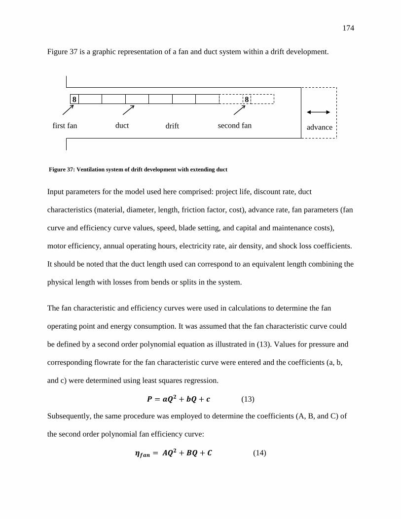
174

Figure 37 is a graphic representation of a fan and duct system within a drift development.

Input parameters for the model used here comprised: project life, discount rate, duct

characteristics (material, diameter, length, friction factor, cost), advance rate, fan parameters (fan

curve and efficiency curve values, speed, blade setting, and capital and maintenance costs),

motor efficiency, annual operating hours, electricity rate, air density, and shock loss coefficients.

It should be noted that the duct length used can correspond to an equivalent length combining the

physical length with losses from bends or splits in the system.

The fan characteristic and efficiency curves were used in calculations to determine the fan

operating point and energy consumption. It was assumed that the fan characteristic curve could

be defined by a second order polynomial equation as illustrated in (13). Values for pressure and

corresponding flowrate for the fan characteristic curve were entered and the coefficients (a, b,

and c) were determined using least squares regression.

𝑷 = 𝒂𝑸𝟐 + 𝒃𝑸 + 𝒄 (13)

Subsequently, the same procedure was employed to determine the coefficients (A, B, and C) of

the second order polynomial fan efficiency curve:

𝜼𝒇𝒂𝒏 = 𝑨𝑸𝟐 + 𝑩𝑸 + 𝑪 (14)

8 8

drift advance first fan second fan duct

Figure 37: Ventilation system of drift development with extending duct

175

The auxiliary ventilation system resistance corresponded to the sum of the duct resistance

(𝑅𝑑𝑢𝑐𝑡), and the equivalent Atkinson resistance from exit and entry shock losses (𝑅𝑠ℎ𝑜𝑐𝑘),

calculated using (15) and (16) respectively. For the purpose of this assessment, the drift

resistance was assumed to be negligible compared to the duct resistance (Duckworth, Lowndes

2003) which was shown by the results from the MTI testing in Table 11, and thus was omitted.

𝑹𝒅𝒖𝒄𝒕 = 𝒌∗𝑳∗𝒑𝒆𝒓𝑨𝟑

(15)

𝑹𝒔𝒉𝒐𝒄𝒌 = 𝑿∗𝝆𝟐𝑨𝟐

(16)

where: 𝑋 was the sum of shock loss coefficients for entry and exit losses

𝜌 was the air density (kg/m3

𝐴 was the duct area (m

) 2

The number of fans required was determined based on the length of the duct, equivalent

Atkinson resistance from exit and entry shock losses, and the maximum length of duct that the

selected fan could handle before entering a stall condition. Equations (16) and (17) were used to

determine the maximum duct length per fan and the number of fans respectively.

).

𝑴𝒂𝒙 𝑳𝒇𝒂𝒏� = (𝑹𝒎𝒂𝒙−𝑹𝒔𝒉𝒐𝒄𝒌)×𝑨𝟑

𝒌×𝑷𝒆𝒓 (17)

𝑵𝒐.𝒇𝒂𝒏𝒔 = 𝑳𝒅𝒖𝒄𝒕𝑴𝒂𝒙 𝑳

𝒇𝒂𝒏� (18)

176

The operating point of a fan was determined by calculating the flowrate corresponding to the

intercept of the fan curve (13) and the system resistance curve (19), in other words the point

where the pressure from both equations was the same.

𝑷 = 𝑹𝑸𝟐 (19)

(𝒂 − 𝑹)𝑸𝟐 + 𝒃𝑸 + 𝒄 = 𝟎 (20)

where: 𝑃 is the pressure (Pa)

𝑅 is the total system resistance (Ns2/m8

𝑄 is the flowrate (m

)

3

𝑎, 𝑏, 𝑐 are the fan characteristic curve coefficients.

/s)

Then solving the quadratic formula in (20) yielded the operating point flowrate. Subsequently,

the operating point pressure could be calculated by substituting this flowrate into (19). Once the

operating point flowrate was calculated it was also possible to calculate the fan efficiency by

substitution of this flowrate into (14).

When multiple fans were installed in series, the flowrate was determined by the intercept of the

system resistance curve and the combined fan curve. This fan curve was constructed by

multiplying the pressure for each flowrate value by the number of fans from the single fan

characteristic curve. Then the pressure and efficiency for the individual fans were determined

from the single composite fan curve. In this treatment it was assumed that the performance of the

additional fans was not affected by its predecessors. Figure 38 shows the system resistance curve

of a duct length exceeding the limit of a single fan by 1 meter. The combined and single fan

curves, and the fan efficiency curve are also plotted.

177

Figure 38: Operation points of single fan and combined fans in series

It can be observed from Figure 38 that for a given system operating at the stall point (X1) the

corresponding pressure, flowrate and efficiency are represented by P1, Q1 and η1 respectively.

However, when the system resistance was increased to 1 meter beyond the limit of the fan, an

additional fan was added to the system. The operating point of this system (X2) was determined

by the intercept of the system resistance curve and the combined fan curve, but the operating

point for the individual fans (X2ʹ) showed that the flowrate (Q2) and the efficiency (η2) were

higher than that of the single fan operating at the stall point, but the pressure (P2ʹ) was lower.

The auxiliary ventilation model was also designed to consider a system equipped with variable

speed fans, thus the required airflow then becomes an input value. Using the fan laws, the fan

10

20

30

40

50

60

70

80

90

0

1,000

2,000

3,000

4,000

5,000

6,000

7,000

0 10 20 30 40 50 60

Fan

effic

ienc

y (%

)

Pres

sure

(Pa)

Flowrate (m3/s)

System resistance (final duct length)

Fan curve

Combined fan curve (fans in series)

Fan efficiency

Q1

X1

X2

X2ʹ

Q2

η1

η2

P1

P2ʹ (each fan)

P2 (total of all fans)

178

speed required to deliver the desired airflow was calculated based on the operating point of the

system at the fan’s maximum speed, illustrated in (21).

𝒏𝟐 = 𝒏𝟏 �𝑸𝟐𝑸𝟏� (21)

where: 𝑛2 is the fan speed required to deliver the requested airflow (rpm)

𝑛1 is the maximum fan speed (rpm)

𝑄2 is the airflow at maximum speed, calculated as the intercept of the system resistance and fan curves (m3

𝑄1 is the desired airflow (m

/s)

3

/s).

Since the input value for the advance rate was in meters per day, the ventilation analysis was

conducted on a daily basis. Capital costs for purchasing the fan and the duct were annuitized to a

daily basis following the equivalent annual cost method from McPherson (1993). Then these

were added to the daily operational cost, which corresponded to the electricity cost incurred for

delivering air through the duct and included the fan and motor efficiencies, also described in

McPherson (1993).

The calculations in this section were repeated on a daily basis until the duct length had reached

the desired value then the total costs were aggregated annually until the project life was expired.

Subsequently, the following output values were computed: annual energy consumption, annual

costs (energy, fan, duct, and total), unit costs ($/m), number of fans required in the system,

minimum, maximum, and average flowrate, average pressure and fan efficiency. The average

flowrate, pressure and efficiency values corresponded to the life cycle weighted average values

179

determined for the duration of the project. Specific cost ($/year)/(m3

8.5 Hypothetical case studies using the ventilation model

/s) was also computed to

compare scenarios and determine the best option for a given situation.

8.5.1 Examination of scenarios with fixed-speed, fixed-custom speed, and variable-

speed fans, for duct lengths up to 1200m

Several case studies were examined with the use of the model presented in the previous section.

The duct materials compared in the assessments were layflat PVC, plastic, and steel, with duct

lengths up to 1200 m. Capital costs for the ventilation systems were computed using the relevant

total duct unit costs ($/m) presented in section 8.4.1, and an estimate of the fan cost obtained

from a supplier. Operational costs included an estimate for fan maintenance, and the calculated

energy costs derived from the model. The layflat PVC and steel friction factors were obtained

from McPherson (1993), whereas the plastic friction factor was the value determined for that of a

smooth pipe with a diameter of 0.6m supplying air to the working face in a 25m2

The first set of case studies was conducted using a fan running at 1800 rpm. This could entail the

use of a fan from an existing inventory, that has been retired from use in an area were mining

was complete. In these scenarios, it was assumed that the ventilation engineer determined that

the airflow supplied by the fan at these settings (blade pitch, and fan speed) would meet or

drift at a

maximum air velocity of 4 m/s. Although this value is lower than that determined with the

ventilation survey results, the purpose of this study was to illustrate the methodology for

assessing ventilation systems with different costs and different duct friction factors. The analysis

was completed for a project life of 1, 3 and 5 years to examine the economics of short-, medium-

, and long-term projects.

180

exceed the ventilation requirements. However, there were no attempts to minimize the excess

airflow and thus surplus energy consumption from this system. Figure 39 illustrates a summary

of the results for a 1 year project using a fixed fan speed of 1800 rpm.

Figure 39: Summary of annual cost versus final duct length for different duct types

Figure 39 was derived from 3 scenarios (one for each duct type), all having the same input

parameters, and each scenario presented the results of individual case studies for duct lengths

ranging from 4 m to 1200 m.

Then another series of scenarios was analyzed, where the minimum flowrate supplied during the

project for all duct types and lengths corresponded to 31 m3

0

1

2

3

4

5

6

0 200 400 600 800 1000 1200 1400

Annu

al co

st ($

/yea

r) x1

00,0

00

Final duct length (m)

Steel total Plastic total Layflat total

Steel energy Plastic energy Layflat energy

/s, the lowest value from the fixed-

181

speed fan scenarios at 1800 rpm. This was achieved by setting the fan speed to a custom value

for each duct type and length. Although the fan speed was adjusted for each case study it should

be noted that it remained constant throughout each project and that at certain points the delivered

amount of air exceeded the minimum requirement. An alternative to adjusting the fan speed

could have been to adjust the fan blade pitch, which would have also shifted the fan

characteristic curve, however to be practical this would require an external method of varying the

pitch which would be more costly. These scenarios were used to mimic a situation where a

ventilation engineer would make use of a fan from an existing inventory, as in the previous

scenarios, but in these cases a one-time adjustment to the fan settings were considered to

minimize energy consumption while meeting airflow requirements.

A third analysis was conducted using a variable-speed fan to maintain a constant flowrate as the

duct was extended. The input parameters were the same as those for the fixed-speed scenarios

however, the fan capital cost was adjusted to include a variable frequency drive (VFD), and the

fan speed input was replaced with a flowrate input. The flowrate selected for this analysis also

corresponded to 31 m3 Table 17/s. shows the input parameters used in the case studies, the values

for duct diameter through to fan maintenance cost were considered common throughout all cases.

182

Table 17: Input parameters for ventilation system analysis

Fixed-speed

(1800 rpm)

Fixed-speed

(custom rpm)

Variable-speed

Duct diameter (m) 1.22

Advance rate (m/day) 4

Layflat PVC friction factor (kg/m3 0.0037 )

Steel friction factor (kg/m3 0.0021 )

Plastic friction factor (kg/m3 0.0011 )

𝑋 (exit and entry shock loss

coefficient)11

1.5

Electricity rate ($/kWh) 0.08

Operating hours (hrs/year) 8760

Motor efficiency (%) 95

Discount rate (%) 10

Average air density (kg/m3 1.22 )

Fan model Alphair 4800-VAX-2700

Fan maintenance cost ($/year) 360

Fan capital cost ($) 30,000 30,000 45,000

Fan speed (rpm) 1800 custom N/A

Flowrate (m3 N/A /s) 31 minimum 31 constant

11 where 𝑋 for exit losses corresponded to 1 and for sharp-edged entry losses was 0.5

(McPherson 1993)

183

Figure 40 summarizes the results for ventilation systems equipped with a fixed-speed, a fixed-

custom speed, or a variable-speed fan, for a project life of 1, 3, and 5 years. The results include

total annual costs (capital and operational) illustrated by the solid lines, and annual energy costs

shown by the dashed lines for all duct types considered in the case studies. It should be noted

that although the analysis was conducted using an advance rate, the results represent the average

annual cost corresponding to projects with various final duct lengths ranging from 4 m to 1200

m. This should not be confused with the life-cycle cost of a duct extended from 4 m to 1200 m.

184

0

1

2

3

4

5

6

0 200 400 600 800 1000 1200

Annu

al co

st ($

/yea

r) x

100,

000


0

1

2

3

4

5

6

0 200 400 600 800 1000 1200

Annu

al co

st ($

/yea

r) x

100,

000


0

1

2

3

4

5

6

0 200 400 600 800 1000 1200

Annu

al co

st ($

/yea

r) x

100,

000


0

1

2

3

4

5

6

0 200 400 600 800 1000 1200

Annu

al co

st ($

/yea

r) x

100,

000


0

1

2

3

4

5

6

0 200 400 600 800 1000 1200

Annu

al co

st ($

/yea

r) x

100,

000


0

1

2

3

4

5

6

0 200 400 600 800 1000 1200

Annu

al co

st ($

/yea

r) x

100,

000


0

1

2

3

4

5

6

0 200 400 600 800 1000 1200

Annu

al co

st ($

/yea

r) x

100,

000


0

1

2

3

4

5

6

0 200 400 600 800 1000 1200

Annu

al co

st ($

/yea

r) x

100,

000


0

1

2

3

4

5

6

0 200 400 600 800 1000 1200

Annu

al co

st ($

/yea

r) x

100,

000


Fixed-speed12

Fixed-custom speed13

Variable-speed14

1

year

pro

ject

3

year

pro

ject

5 ye

ar p

roje

ct

Figure 40: Total and energy costs for ventilation systems of various duct materials and lengths

12 Use of a fan from an existing inventory, such as one that is retired from use in an area where mining is complete, without consideration of the fan settings.

13 Use of the same fan as with the fixed-speed, 1800 rpm scenarios, but fan speed is set such that the minimum air supply meets requirements, but the speed is constant throughout the project.

14 Use of the same fan as other case studies but a variable frequency drive is added to control the fan speed and maintain a constant airflow throughout the project.

Steel total Plastic total Layflat totalSteel energy Plastic energy Layflat energy

a)

b)

c)

d)

e)

f)

g)

h)

i)

185

Throughout Figure 40 it can be seen that the plastic duct system consumed the least amount of

energy for all scenarios, regardless of the project duration or fan settings. The steel duct was the

second lowest energy user and the layflat was the highest energy consumer. This is to be

expected as it is directly related to the friction factor. The relative differences were small on the

shorter duct lengths where the entry and exit losses common to each were more dominant. The

relative spacing between the energy use profiles also varied as a function of length, reflecting the

differences in the number of fans employed. Also, as might be expected, as the project duration

increased, the proportion of total costs attributed to energy costs increased for each duct type at

corresponding duct lengths.

From the simulation results shown in Figure 40a, it can be seen that the most costly option

overall corresponded to the plastic system for all duct lengths, despite its energy cost being the

lowest. However which was cheapest depended on the final duct length. Up to 292 m, the option

with the lowest total cost was the layflat PVC duct, but at a duct length of 292 m through to 515

m where the layflat PVC needed a second fan the steel system became the cheapest. At this

distance the steel system required an additional fan and the layflat PVC again became the lowest

cost option. Despite the addition of fans to both systems at longer lengths, the layflat PVC duct

remained the cheapest to 1200 m.

Throughout panels a to f of Figure 40, it can be seen that whether a certain duct has the lowest

combined operating and capital cost, is the most expensive or is comparable is very dependent on

the step changes, corresponding to the requirement of supplementary fans in the ventilation

system. These figure panels (a to f) also show that the step change becomes less significant for

longer duct lengths as the operating cost (energy) becomes more dominant. The cause of these

notable step changes in panels a to f is two-fold: the obvious increase in capital cost for

186

purchasing the additional fan, and then an increase in operational cost as a result of the system

supplying higher flowrates than required when the fans are combined in series, as exemplified

previously in Figure 38. At the change over point, the increased flowrate increased the power.

Although the pressure was lower and the efficiency was higher than that of the single fan at the

stall point, these differences were not sufficient to overcome the effect of the increased flowrate

when a second or third fan was added, due to the cubic relation between the power and the

flowrate.

Comparing panels a to c of Figure 40 highlights the time factor and that energy becomes more

dominant in the long-term. It can be observed from Figure 40b that all options had similar costs

up to 50 m and that the steel and layflat options were comparable up to 80 m but the lowest cost

option was the layflat PVC duct up to a length of 292 m. At this point where an additional fan

was added to the layflat PVC system, the steel option was the lowest cost up to a duct length of

515 m. Then when an additional fan was added to the steel system, the plastic duct still operating

with one fan became the most economical solution until it needed a second fan. The lowest total

cost system for these scenarios alternated between the steel and plastic ducts with the addition of

supplementary fans in each system. The steel was cheaper where both systems employed the

same number of fans, while the plastic was cheaper as long as it needed less fans.

Figure 40c shows that the economics for a 5 year project with a fixed-speed fan at 1800 rpm

were similar to those of the 3 year project. For short systems employing one fan the difference

between the various types of duct are even less significant. The layflat PVC is the lowest cost

system up to 292 m then the steel option becomes the cheaper system while the layflat PVC

required an additional fan. Beyond 515 m the lowest cost option would be plastic ducting as long

as it required less fans than the other systems.

187

In Figure 40d through f where the fan has been set to a customized fixed duty, it can be observed

that the lowest total cost options for the shorter duct length and project life scenarios alternated

between the layflat PVC and steel ducts depending on the number of fans required in the

systems. However as for the fixed speed fan, steel and plastic would be the preferred choice for

longer length and life systems. The plastic duct increasingly becomes the low cost option with

the longer project life and longer length when it required less fans. As shown in Figure 40f, the

plastic duct was the most economical up to 956 m and beyond 1160 m.

Figure 40g through i show the benefits of systems with a fixed delivery provided by variable

speed fans. Throughout, the step changes incurred on introducing additional fans are less

significant. This indicates that the capital cost of the fan is less of a factor compared to the

additional flow provided in the previous two fixed duty scenarios. These figures also show that

the cost benefit of one type of duct over another can be less distinct with volume control.

Figure 40g shows that the plastic system was the most expensive option at all duct lengths for a 1

year installation life. A similar low cost alternating pattern was observed between the layflat

PVC duct and the steel duct depending on the number of fans in the systems up to 515 m beyond

which the layflat PVC system remained the lowest cost option regardless of when fans were

added to this system. This figure also shows that the energy cost did not rise as abruptly as in the

fixed-speed fan scenarios due to maintaining a constant flowrate, and thus controlling the power.

The energy step function can also be reversed, through Figure 40 g to i, it can be seen that the

addition of an extra fan can reduce the overall annual operating cost (energy) compared to

operating a fan or fans near their stall condition at low efficiency.

188

As the life of the installation lengthens from 1 to 3 and then 5 years, the layflat PVC clearly

becomes the least attractive. For the 3 year case study, the most economical solution alternates

between the steel and plastic options. For the 5 year project, when the energy costs start to

dominate, the plastic system was the lowest cost option for all duct lengths beyond 200 m.

Overall these figures show that the choice of ducting type should be reasonably straightforward

for a long term project where a constant flow is maintained, especially for long installations.

However, where less concern is given to providing the appropriate flow, the optimum selection

becomes more orientated to the system using the lowest number of fans.

8.5.2 Flow variability

The hypothetical case studies with a fixed-speed fan (either at 1800 rpm or at a custom speed

selected to deliver the minimum flowrate) supplied varying flowrates for each duct type at a

specific length because of the different resistances of the materials. This is illustrated in Figure

41 which shows the system resistance curves for a 200 m layflat PVC, steel and plastic duct.

Each resistance curve intersects the fan curve at a different point with a different associated

efficiency.

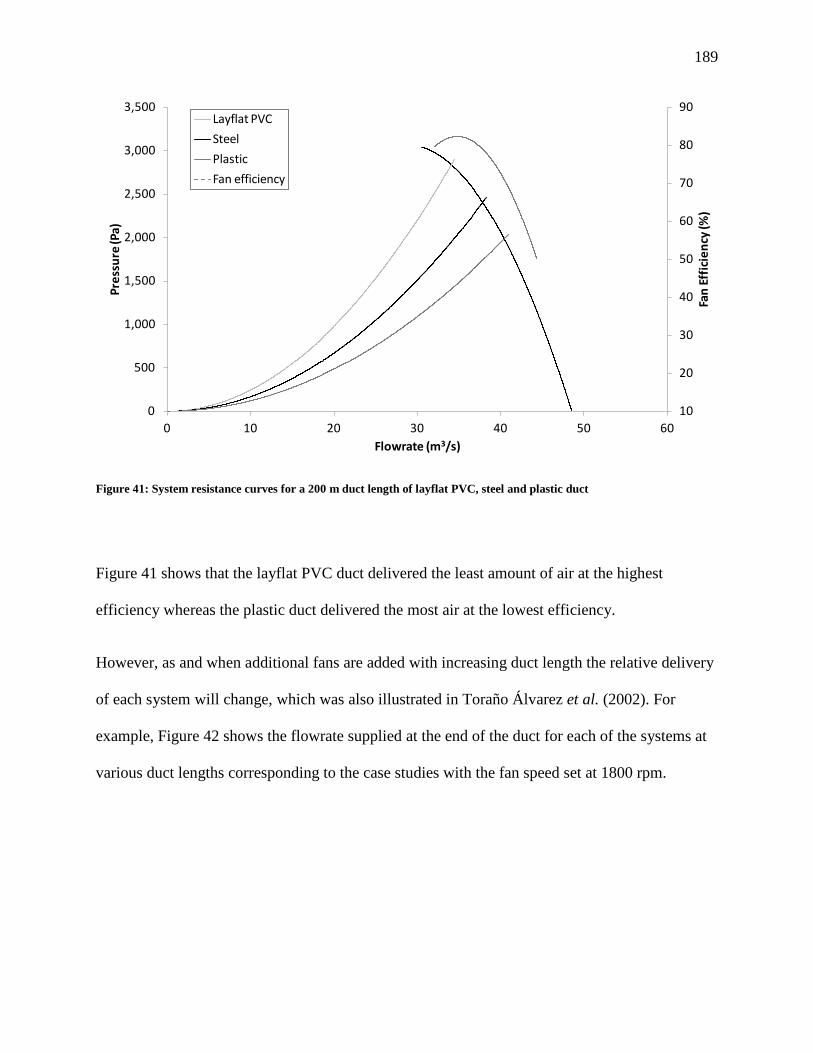
189

Figure 41: System resistance curves for a 200 m duct length of layflat PVC, steel and plastic duct

Figure 41 shows that the layflat PVC duct delivered the least amount of air at the highest

efficiency whereas the plastic duct delivered the most air at the lowest efficiency.

However, as and when additional fans are added with increasing duct length the relative delivery

of each system will change, which was also illustrated in Toraño Álvarez et al. (2002). For

example, Figure 42 shows the flowrate supplied at the end of the duct for each of the systems at

various duct lengths corresponding to the case studies with the fan speed set at 1800 rpm.

10

20

30

40

50

60

70

80

90

0

500

1,000

1,500

2,000

2,500

3,000

3,500

0 10 20 30 40 50 60

Fan

Effic

ienc

y (%

)

Pres

sure

(Pa)

Flowrate (m3/s)

Layflat PVCSteelPlasticFan efficiency

190

Figure 42: Supplied flowrate versus final duct length for fixed speed fan at 1800 rpm

This figure shows that substitution of one type of duct for another for a given fan could lead to

varying degrees of over-supply of air for a given duct length. With consideration given to

specific fan settings, the oversupply of the steel and plastic ducts would be less than that of the

layflat as long as these systems are operating with a single fan. With a variable speed ventilation

system the minimum flow would be maintained throughout.

Consequently, fixed-custom speed and variable speed systems should consume less energy than

the fixed-speed 1800 rpm scenarios at corresponding duct lengths and project durations. This

illustrates the important fact that the selection of the lowest energy consuming duct based on a

lower friction factor despite maximizing energy savings may not give the most cost effective

solution. Thus when a fan is taken from an existing inventory, it is imperative that the fan

0

5

10

15

20

25

30

35

40

45

50

0 200 400 600 800 1000 1200 1400

Flow

rate

(m3 /

s)


Layflat PVC

Steel

Plastic

Minimum flowrate limit

191

characteristics are examined to determine: i) whether the fan is suited for this situation, and ii)

whether the fan settings are optimal to minimize operational costs.

8.5.3 Potential energy savings

Energy savings in auxiliary ventilation systems can be achieved by controlling the air flow or by

substitution of a duct with one having a lower friction factor. Figure 43 and Figure 44 shows the

potential energy savings of the fixed-custom speed fan and the variable-speed case studies

compared to their fixed-speed 1800 rpm counterparts throughout their advance and while at

maximum extension for the duration of the project.

Figure 43: Energy savings for fixed custom speed fan compared to fixed speed stock fan for 1 year project

0

10

20

30

40

50

60

70

0 200 400 600 800 1000 1200

% e

nerg

y sa

ving

s


Layflat PVC Steel Plastic

192

Figure 44: Energy savings for variable speed fan compared to fixed speed stock fan for 1 year project

The lowest energy savings for both the fixed-custom speed and variable-speed fans occurred at

duct lengths where a second fan was added to each of the systems. There were no savings for the

fixed-speed system compared to the one with the fan at 1800 rpm when a second fan was added

because at a certain design length both systems would have fans operating at 1800 rpm and

delivering the same amount of air, thus the operating points of these systems were the same

throughout the duration of the project.

0

10

20

30

40

50

60

70

0 200 400 600 800 1000 1200

% e

nerg

y sa

ving

s


Layflat PVC Steel Plastic

193

The maximum savings occurred at the shortest length, because the largest fan speed reduction

compared to the fixed-speed fan at 1800 rpm occurred at the shortest length, and correspondingly

the larger reduction in airflow between systems.

Figure 43 and Figure 44 also illustrates that proper speed selection for a fixed-speed fan can

deliver similar energy savings than with the use of a variable-speed fan compared to the fixed-

speed stock fan option. At the shortest duct lengths, the energy savings between these systems

were comparable for a given duct type, however the savings between these systems increased

with duct length. For example, the energy savings for a 100 m plastic duct was 62% for both the

fixed-custom speed and variable-speed fan systems compared to the fixed-speed stock fan. For a

500 m plastic duct the energy savings corresponded to 39% with the use of a fixed-custom speed

fan, and 44% with the variable-speed fan, thus the additional savings for the variable-speed

system was 5%. However, the energy savings for a 800 m plastic duct were 16% and 31%, thus

the variable-speed option provided an additional 15% energy savings. The energy savings

increased with duct length for two reasons. First, at a short duct length, the range of fan speed for

a variable-speed fan to maintain a constant airflow was less than for a longer duct, thus the

savings were minimal. Second, although the fixed-custom speed fan systems delivered more air

than that required at the start of the projects, once the final duct length was reached they operated

at the same operating point as the variable-speed systems. For short ducts, this point was reached

quicker therefore the energy consumption was mainly influenced by the final operating point,

which was the same for these systems.

Another option to reduce energy consumption would be through the use of a lower friction duct

while keeping the same fan. Figure 45 illustrates the potential energy savings of substituting the

layflat PVC duct with plastic for a 1 year project.

194

Figure 45: Energy savings from substitution of a layflat duct for a plastic duct for 1 year project

For plastic substitution with a fixed custom speed fan the savings increase when additional fans

are introduced in the layflat system because of the increased flowrate when a fan is added. The

savings were reduced when a second fan was added to the plastic duct system for the same

reason. The maximum savings from substitution of the layflat duct with a plastic one with a

fixed-speed fan corresponded to 58%.

In the custom-speed scenarios, the maximum savings from duct substitution corresponded to

74% and occurred at the duct length where a second fan was added to the layflat system, the

reason again being the increased flowrate. At duct lengths greater than 956 m, both the layflat

0

10

20

30

40

50

60

70

80

0 200 400 600 800 1000 1200

% e

nerg

y sa

ving

s


Fixed speed fan Custom speed fan Variable speed fan

195

and the plastic systems have fans operating at 1800 rpm to supply the design flowrate, thus the

savings for these lengths are the same as for the fixed-speed fan scenarios.

In the variable-speed scenarios the savings increased with duct length, where small reductions in

savings were observed when additional fans were introduced in the layflat system because of the

higher fan efficiency. The maximum energy savings corresponded to 63% and occurred at the

longest duct length examined in the scenarios.

The energy savings in the fixed-speed fan scenarios were greater than those with the variable-

speed fan when more than one fan was used in the layflat system because the excess flowrate,

resulting from introduction of additional fans, was controlled in the variable-speed option.

Although duct substitution and flowrate control provide measures for energy savings, the use of

both strategies would maximize energy conservation in auxiliary mine ventilation systems.

Figure 46 shows the annual operating costs, corresponding to electricity costs for the various

duct types examined in the case study using a fixed speed fan compared to the plastic option

where the flowrate was controlled for a 1 year project.

196

Figure 46: Energy costs from duct substitution and flowrate control for 1 year project

Figure 46 shows that although the plastic duct consumed less energy than the other duct types

with a fixed speed fan, the energy use was lessened when the flow rate was controlled. For short

duct lengths the energy consumption between the fixed custom speed and variable speed options

were similar. As the duct length increased, the energy savings from the variable speed system

increased because the fixed custom speed fan delivers excess air until the final duct length is

reached, which occurs later for longer ducts.

Project duration also influenced the annual operating costs as illustrated in Figure 47 and Figure

48.

0

0.5

1

1.5

2

2.5

3

3.5

0 200 400 600 800 1000 1200

Ope

ratin

g co

st ($

/yea

r) x

100,

000


Layflat PVC (Fixed speed) Steel (Fixed speed)

Plastic (Fixed speed) Plastic (Fixed custom speed)

Plastic (Variable speed)

197



0

0.5

1

1.5

2

2.5

3

3.5

0 200 400 600 800 1000 1200

Ope

ratin

g cos

t ($/

year

) x10

0,00

0





0

0.5

1

1.5

2

2.5

3

3.5

0 200 400 600 800 1000 1200

Ope

ratin

g cos

t ($/

year

) x10

0,00

0





198

It can be observed from Figure 47 and Figure 48 that the lower friction plastic duct with flowrate

control options consumed the least amount of energy. However, the difference between the fixed

custom speed and variable speed fan systems with one fan was reduced because both systems

were at the same operating point for longer durations. The variable speed fan provided energy

savings via flowrate control as the duct was being extended but once the final duct length was

reached both systems operated at the same speed. As the project life lengthened the proportion of

time corresponding to the installation period where the duct length was extended was smaller;

thus the energy savings were reduced. The advantage of the variable speed system occurred in

systems with more than one fan by minimizing the discontinuity introduced by the excess

flowrate when additional fans were added to the fixed custom speed system.

Energy savings can be obtained in auxiliary mine ventilation systems by substitution of the duct

with one with a lower friction factor, or by controlling the excess flowrate in a given system but

energy savings could be maximized with the use of both measures. Figure 49 compares the

potential energy savings of the individual and combined measures.

199

Figure 49: Potential energy savings from duct substitution and flowrate control

In Figure 49, the “Layflat (Fixed speed) vs Plastic (Fixed speed)” series demonstrated that the

potential energy savings from duct substitution varied from 1% to 58% depending on the final

duct length. The “Layflat (Fixed speed) vs Layflat (Variable speed)” series illustrated the

potential energy savings from flowrate control, ranging from 7% to 66%. It can be observed that

the potential for energy savings, ranging from 56% to 74% was greater when both energy

conservation measures were combined, shown by the “Layflat (Fixed speed) vs Plastic (Variable

speed)” series.

8.5.4 Capital cost versus energy savings

Although the steel and plastic installations consumed less energy, the higher capital costs for

these systems in certain scenarios presented an obstacle to ranking these materials as the lowest

0

10

20

30

40

50

60

70

80

0 200 400 600 800 1000 1200

% e

nerg

y sa

ving

s


Layflat (Fixed speed) vs Plastic (Fixed speed)Layflat (Fixed speed) vs Layflat (Variable speed)Layflat (Fixed speed) vs Plastic (Variable speed)

200

cost option. Regardless of the type of system (fixed-speed or variable-speed fan), for short-term

projects, the energy savings were not sufficient to recover the higher capital cost of the plastic

duct. For medium and long-term projects, the economic viability of the lower energy cost

systems was improved, and for some duct lengths the plastic system was the lowest cost option.

The variable-speed ventilation systems investigated within the case studies that had lower energy

costs than their fixed-speed counterparts were due to the flowrate control which lowered the

energy consumption. However, for short duct lengths, the fixed-custom speed scenarios had

lower total costs for all projects for two reasons. First, the capital cost increased because an

additional $15,000 was incurred for the purchase of the VFD, corresponding to a fan capital cost

increase of 50%. Second, the range of flowrate values, between the start of the duct and the final

design length as supplied from fixed-custom speed systems, was small for short ducts. Thus

where the excess flowrate was small, the energy savings directly related to flow were similarly

small.

For fixed-speed systems, the addition of supplementary fans leads to an increased flowrate,

resulting in higher energy cost. In some instances, this increase was sufficient to alter the ranking

of options based on total cost.

Thus when capital costs are included, the lowest energy system may not be the cheapest option;

energy use, capital costs and project duration are variables that influence the economic viability

of the various systems.

201

Figure 50: Annual costs from duct substitution and flowrate control for 1 year project


0

1

2

3

4

5

6

0 200 400 600 800 1000 1200

Ann

ual c

ost (

$/ye

ar) x

100,

000





0

1

2

3

4

5

6

0 200 400 600 800 1000 1200

Ann

ual c

ost (

$/ye

ar) x

100,

000





202


From Figure 50 it can be observed that for a 1 year project, although the energy use was

minimized with use of the plastic duct and flowrate control, these systems were the lowest cost

options for short duct lengths only. However from Figure 40 it was shown that the steel and

layflat PVC systems were cheaper than the plastic option with flowrate control. Thus regardless

of whether the energy savings were maximized via flowrate control, the economics did not favor

the plastic system.

For the 3 year project options illustrated in Figure 51 it can be seen that the cheapest option

corresponded to the plastic system with flowrate control. For systems with one fan, the cost of

the variable speed and fixed custom speed fan options were comparable, but the variable speed

0

1

2

3

4

5

6

0 200 400 600 800 1000 1200

Ann

ual c

ost (

$/ye

ar) x

100,

000





203

fan system was the cheaper option with two fans. However, from Figure 40 it was observed that

for fixed custom speed systems the cost of the steel and plastic systems were comparable when

both options had only one fan. Conversely, the costs of the steel and plastic systems with

variable speed fans were comparable for all duct lengths. Thus the lowest cost system in these

scenarios corresponded to the steel or plastic duct with either a fixed custom speed or a variable

speed fan with one fan installed in the steel system. When a second fan is introduced in the steel

system the fixed custom speed option cost rose above the other system costs and left the plastic

duct with a fixed custom speed fan and the steel and plastic ducts with variable speed fans

competing for the lowest cost. Subsequently, the addition of a second fan in the plastic system

eliminated the fixed custom speed scenario from the lowest cost options, thus only the steel and

plastic systems with a variable speed fan remained for longer duct lengths.

In Figure 52 it can be observed that for a 5 year project the lowest cost options corresponded to

the use of a plastic duct with either a fixed custom or variable speed fan when the system only

required one fan. When a second fan was added, the cost of the plastic system with a variable

speed fan was the lowest. But from Figure 40 it was observed that the costs of the steel duct with

a fixed custom speed or a variable speed fan were comparable to that of the corresponding plastic

systems for short duct lengths. Thus the lowest cost option corresponded to either of these four

systems. For duct lengths greater than 200 meters the cost of the plastic system operating with

only one fixed custom speed fan was lower than its steel counterpart. When a second fixed

custom speed fan was added to the plastic system, the steel option was cheaper however the cost

of the plastic duct with a variable speed fan system was even lower.

As there are a large number of possible scenarios that can exist, it was not possible to examine

every plausible situation; therefore the model used in this study has been made available for

204

individual users to explore custom scenarios and to assist in determining the optimal solution for

a given mine ventilation system, whether the objective is to choose the lowest cost or lowest

energy consumption option (Levesque, Millar 2015a).

8.6 Examination of leakage effects on ventilation survey results

A subsequent model was developed to investigate the effect of leakage in auxiliary mine

ventilation systems. The leakage model retained the feature to model a duct as a drift is extended

from the original leak-free model but to determine the operating point of the fan, an equivalent

system resistance is calculated using a series-parallel methodology based on that presented in

Vutukuri (1983).

8.6.1 Series-parallel theory and resistances

The resistance of the various components in an auxiliary ventilation system can be connected in

series or in parallel. Figure 53 illustrates a ventilation system with the following components: an

inlet bell (blue), a fan (green), and four duct segments (yellow) which are installed in a drift. In

this simple system, the leakage at the joints between the components may be considered to be

connected in parallel between the duct and the drift. The jagged lines in the diagram represent

the resistance of the various components; Rd1 is for the inlet bell, Rd2 is for the fan, Rd3 to Rd5

are for the duct segments, Rsh =R7 is for the exit shock loss, Rb1 to Rb5 is for the drift, and Rj1 to

Rj5 are for the leaks.

205

Figure 53: Schematic of series-parallel theory in an auxiliary ventilation system

The resistance for each drift and duct segment is calculated using (8) and (15) respectively

(McPherson 1993). The exit shock loss is calculated as (16) where X corresponded to a value of

1 and the inlet bell resistance was also calculated by (16) but the value of X was 0.03

(McPherson 1993) . A resistance value for the leakage paths is entered as an input to the model

where the resistance for all leakage paths is assigned this value. However, any of the individual

leakage resistance values can be overwritten to simulate a poor joint or a very good seal at any

location in the system. All resistance values have the units of Ns2/m8

.

206

Calculation of the resistance for a system with components in series corresponds to the

mathematical sum of the individual resistances. However, for parallel resistances, the system

resistance is calculated using (22) from McPherson (1993).

𝟏�𝑹𝒑𝒂𝒓

= ∑ 𝟏√𝑹

(22)

Calculation of the system resistance for the simple ventilation system in Figure 53 which

comprised resistances in series and in parallel proceeded as follows, and is illustrated in Figure

54.

1. Calculations begin by calculation of the last branch, represented by R6

2. The resistances of the last duct segment (R

at the end of the

duct.

d6), the exit shock loss (Rsh=R7), and that of

the drift segment (Rb6

3. Then R

) are summed since these are joined in series.

j6 is added to the calculations but this resistance is in parallel with those from step

2, thus 1�𝑅6

= 1

�𝑅𝑗6+ 1

�𝑅𝑑6+𝑅𝑠ℎ+𝑅𝑏6 where R6

4. R

is considered the equivalent resistance of

the last branch.

6, Rd5 and Rb5 are connected in series and thus are summed, but the sum of these is in

parallel with Rj5

5. The procedure continues until the resistance of all of the branches has been characterized

by one equivalent resistance value represented by R

, thus the equivalent resistance of the last two branches in the system is

calculated using 1�𝑅5

= 1

�𝑅𝑗5+ 1

�𝑅𝑑5+𝑅𝑏5+𝑅6

1 Figure 54 in the bottom frame of .

207

Figure 54: Schematic illustrating the steps to calculate the equivalent resistance of a series-parallel ventilation system

208

The fan operating point can then be determined by the intercept of the fan curve and the system

equivalent resistance curve. Pressure and flowrate values are also calculated for each segment

within the ventilation system.

8.6.2 Case studies of auxiliary ventilation systems with leaky joints

The leakage model was subsequently used to compare different auxiliary ventilation systems

with low, medium, and high friction factor ducting with different degrees of leakage; the leakage

in the case studies was assumed to be uniform throughout the system. Use of the model allowed

simulation of values that would be obtained during a ventilation survey which could be used to

determine a duct friction factor— as was done at MTI’s Test Mine. Table 18 shows the input

parameters used for all the simulated ventilation systems compared using this leakage model.

Table 18: Common input parameters for all simulated ventilation systems with leakage

Variable Parameter

Fan Alphair 4800-VAX-2700

Drift length (m) 210

Duct diameter (m) 1.2

Duct length (m) 200

Distance from the start of the system for first measurement location (m)

26

Distance from the start of the system for second measurement location (m)

170

209

A total of six ventilation systems were simulated with the model with various combinations of

duct friction factors and joint resistance (Rj

The input value used to characterize leakage in auxiliary ventilation models corresponds to the

resistance of leakage paths (𝑅𝐿) (Vutukuri 1984, Mine Ventilation Services 2003). This quantity

can be determined from pressure and flowrate values obtained during ventilation surveys or from

a ‘leakage coefficient’ (𝐿𝑐) value determined from a nomogram for metal ducts (Le Roux 1979)

but this method also requires knowledge of flowrates and pressures in a given ventilation system.

The leakage coefficient according to Vutukuri (1983) corresponds to the amount of air in m

) values.

3

𝑹𝑳 = 𝟏𝟎𝟎𝟎𝑳𝒄𝟐

(23)

/s

that would leak from a 100 m duct under a uniform pressure of 1kPa and the relationship

between 𝐿𝑐 and 𝑅𝐿 is shown in (23).

Conversely, the definition of 𝐿𝑐 presented in LeRoux (1979) was the amount of air in m3

Thus the values chosen for 𝑅𝐿were determined by calibrating the model against expected leakage

amounts from mine ventilation systems as reported by DeSouza (2004); it was stated that

approximately 0.09 m

/s that

would leak from 1000 m of ducting at 100 Pa. Although these definitions of 𝐿𝑐 differ they both

define the leakage at a given pressure for a given length but the amount of air that leaks from a

duct is influenced by the difference in pressure between the inside and outside of the duct among

other factors such as the number of joints (Wu, Gillies 2014). But the number of joints in a given

duct length will vary depending on the duct segment length and since the number of joints in

each of these definitions was unknown it was not considered prudent to use these

characterizations in the model developed herein.

3/s is expected to leak per joint and that leakage should not exceed 10% of

210

the initial air volume but leakage values exceeding 50% of the initial flow have been observed.

Consequently it was decided to use a leakage value of 10% to define a low leakage system and a

value of 50% for a high leakage system in the model.

A value of 300,000 Ns2m8 for Rj which was considered for the low leakage systems, resulted in

an average flow volume loss of 11% of the initial flow at the fan all duct systems examined in

the model, and average leakage of 0.07 m3/s per joint. For the high leakage systems a value of

4000 Ns2m8 for Rj

Table 19

resulted in average leakage of 55% for all duct systems examined in the

model. The results for the low and high leakage systems are presented in and Table 20

respectively. Pressure and flowrate values at the same 2 locations within the system were

obtained from the simulations for all cases examined, illustrated by P1 and P2 in Figure 55.

These were then used to calculate a duct friction factor value simulating the methodology

described in 7.3.1 employed at the MTI Test Mine. Three friction factor values were calculated,

varying in the method and location of flowrate determination as follows:

• k_Q1 used the flowrate measured at the first location (Method A),

• k_Q2 used the value at the second location (Method B), and

• k_Qavg used the average of the flowrate values observed at both measurement locations

(Method C).

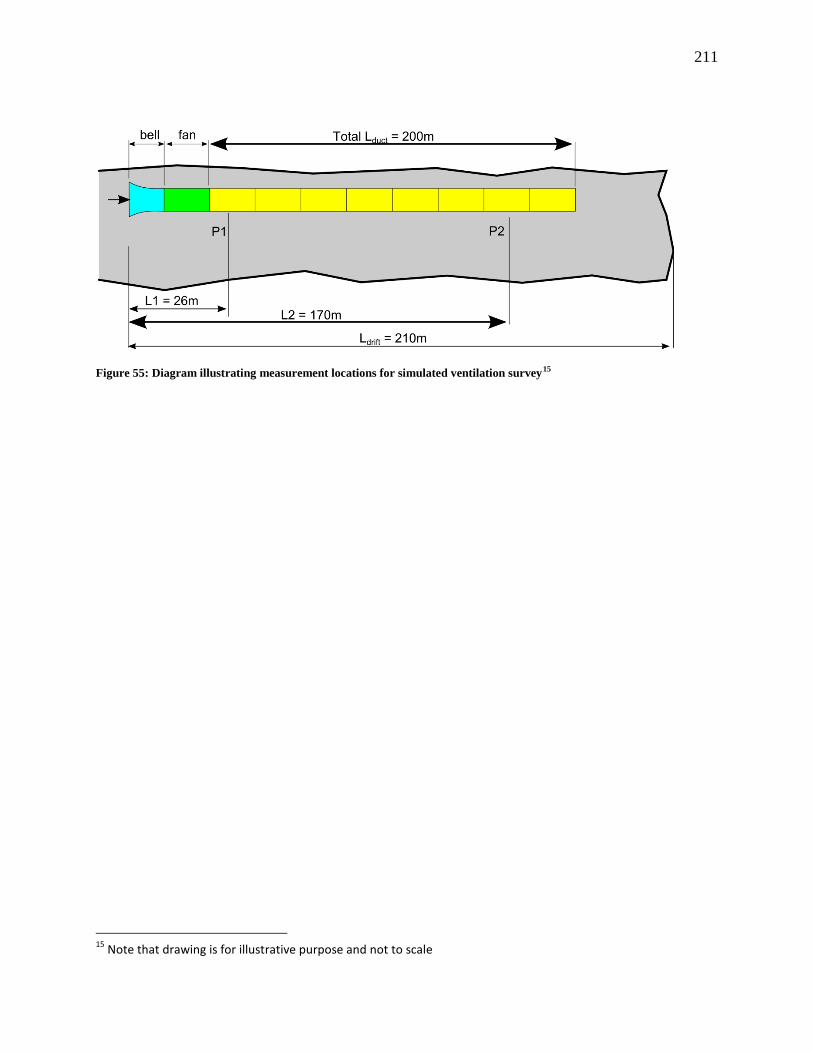
211

Figure 55: Diagram illustrating measurement locations for simulated ventilation survey15

15 Note that drawing is for illustrative purpose and not to scale

212

Table 19: Leakage model results for low leakage systems

Low friction Medium friction High friction

Rj (Ns2/m8 300,000 (low leakage) )

k duct (kg/m3 0.0011 ) - specified 0.0021 0.0037

Req (Ns2/m8 0.9089 ) 1.3412 2.0105

Fan pressure (Pa) 1,639 2,129 2,639

Fan flowrate (m3 42 /s) 40 36

Face flowrate (m3 38 /s) 35 31

Flowrate loss (%) 9.5 10.9 12.7

Airpower (kW) 69 84 95

P1 (Pa) 1,492 1,915 2,351

P2 (Pa) 824 814 786

Q1 (m3 42 /s) 39 35

Q2 (m3 39 /s) 36 32

Back calculated values of k

k_Q1 (kg/m3 0.0010 ) 0.0019 0.0033

k_Q2 (kg/m3 0.0012 ) 0.0023 0.0041

k_avg (kg/m3 0.0011 ) 0.0021 0.0037

Comparison of the known duct friction factor (2nd Table 19 row in ) with those back calculated

using the simulated observations show that use of Method A will result in underestimation of the

duct friction factor, whereas use of Method B leads to overestimates of the duct friction factor.

213

Table 20: Leakage model results for high leakage systems

Low friction Medium friction High friction

Rj (Ns2/m8 4,000 (high leakage) )

k duct (kg/m3 0.0011 ) - specified 0.0021 0.0037

Req (Ns2/m8 0.4293 ) 0.6234 0.8916

Fan pressure (Pa) 1,004 1,340 1,732

Fan flowrate (m3 45 /s) 44 42

Face flowrate (m3 22 /s) 20 17

Flowrate loss (%) 50.1 54.9 60.3

Airpower (kW) 45 58 72

P1 (Pa) 743 987 1,262

P2 (Pa) 290 259 227

Q1 (m3 41 /s) 39 37

Q2 (m3 25 /s) 22 19

Back calculated values of k

k_Q1 (kg/m3 0.0007 ) 0.0012 0.0020

k_Q2 (kg/m3 0.0019 ) 0.0040 0.0079

k_avg (kg/m3 0.0011 ) 0.0021 0.0036

For ventilation systems with high leakage, estimation of the duct friction factor from either

Method A or Method B resulted in a larger error that those from the low leakage systems but the

estimate using the average flowrate (Method C) still provided a good estimate.

Comparison of the equivalent resistance values (Rsys) of the low leakage systems with those from

the corresponding high leakage ducts reveals that increased leakage results in lower system

214

resistance values. The fan operating point is determined by Rsys

Table 13

which comprises resistance of

the drift, the duct, leakage and shock losses, thus it is important to quantify the leakage in a

system when using survey results for more accurate determination of a duct friction factor unless

flowrate determinations are done at both ends. For example, if one measured 2 pressure values

and 1 flowrate in a leaky system but assumed that the installation was leak free, the calculated

duct friction factor may be over or underestimated depending on the location of the flowrate

measurement. Thus these simulations and the different methods used to calculate the duct

friction factor may explain the appreciable variability of reported k factors, which should be an

intrinsic material property, for plastic ducting presented in .

Wu and Gillies (2014) stated that canvas or fabric materials used for fabrication of ventilation

ducts leak due to the porous nature of these materials, thus it was suggested that the use of lower

leakage materials in ventilation systems will lower fan operating costs compared to higher

leakage materials.

The data from the leakage models presented in Table 19 and Table 20 support this notion but it

only applies when considering equal flowrate amounts at the face for each case. For example, if

we consider a low leakage system with a low friction factor it can be seen that the airpower

required corresponded to 69 kW which supplied 42 m3/s through the fan but only 38 m3/s at the

face. Conversely, the high leakage system with a high friction factor required 72 kW to supply

42 m3/s through the fan but only delivered 17 m3/s at the face. Although the amount of air

delivered at the face varied substantially between these systems, the amount supplied by the fan

was the same. Thus in drifts with activities requiring fresh air only at the face it is possible that

the amount of air reaching the working area in the high leakage duct may not be sufficient and

would require more power to increase the air supply. However, in situations where activities

215

requiring fresh air are occurring at various areas along a development drift, it may be acceptable

that the high leakage duct distributes the fresh air where it is required. Both of these systems may

be adequate to meet the demand requirements for fresh air, and would require similar power, but

the meaning of ‘adequacy’ alters between the cases.

8.7 Discussion of auxiliary ventilation systems and friction factors

An Atkinson friction factor for the plastic ventilation duct was calculated using two methods.

The ventilation survey resulted in a value of 0.0020 kg/m3 but although the these values were

repeatable, which provided an indication of the precision, it was unknown whether the values

obtained were accurate. Calculation of the Atkinson friction factor from material roughness

yielded a value of 0.0011 kg/m3

The microscopic images of the duct material samples revealed that the roughness or asperity

height of the plastic material was primarily influenced by the coating applied to the surface.

Therefore, any inconsistencies with the application of this substance could alter the roughness

and thus the friction factor. Alternatively, different application methods could be investigated to

ensure consistent surface coverage, which if smoother than the current application technique

could lead to a lower Atkinson friction factor.

, thus this introduced uncertainty with the values obtained during

the survey.

Although the method employed for the determination of the asperity height in this study may not

have been the most accurate since it was subject to subjective identification of focus points, it did

provide an estimate of the order of magnitude for the roughness. The material samples could

have been examined by scanning electron microscope for a more accurate assessment but it was

not deemed necessary for the purpose of this study. Even if the maximum asperity height value

216

was tripled from 8 µm to 24 µm, the Atkinson friction factor would only increase to 0.0013

kg/m3

Examination of a Moody chart revealed that the roughness of the plastic ventilation duct as

determined by the surface roughness examined with the microscope approached that of a

hydraulically smooth pipe, thus the possibility for ventilation ducts with even lower friction may

be non-existent. It should be noted that although the flow measured during the MTI survey

reached the requirement to be turbulent, according to the Moody chart it was not fully turbulent,

consequently the friction factor can also be dependent on the Reynolds number, which may

provide an explanation for the discrepancy between the values determined with the asperity

height and those from the ventilation survey. It was shown in

, which is still lower than that of other duct materials such as steel or layflat, as well as that

determined from the ventilation survey at MTI.

Table 15 that the Atkinson friction

factor values for a smooth pipe corresponded to 0.0016 to 0.0018 kg/m3 for the range of

Reynolds number values corresponding to those calculated from the ventilation survey data.

Thus the value of 0.0020 kg/m3

It was also shown that the minimum friction factor value for a smooth pipe corresponded to

0.0009 kg/m

also indicates that the friction factor value as determined during

the survey approached that of a smooth pipe.

3, but some values reported for plastic ducting were lower than this minimum. The

examples presented in 7.6 from the leakage model may be used to explain this discrepancy; it

was shown that use of the average flowrate value between 2 measurement locations would

provide a good estimate of the duct friction factor, however use of the flowrate value as

measured at the first location would result in underestimation, which was greater in leaky

systems.

217

The analysis presented demonstrated that although the installation of ducts with lower friction

factors can lead to reduced energy consumption it is also important to consider the fan and duct

as a system to maximize these energy savings, and overall costs. For example, all else being

equal in a given fixed-speed fan ventilation system, the substitution of a lower friction factor

duct can result in an increased flowrate. Although the resulting energy consumption can be

lower, the energy savings would be maximized if the fan speed was reduced to supply the

required amount of air only. This would allow a faster recovery of the higher capital cost for the

plastic duct and render it a financially viable project given sufficient time. Therefore, to

maximize the energy savings from duct material substitutions, either the fan speed, the blade

setting or the fan itself needs to be changed to a lower duty while still ensuring that the minimum

flowrate requirements are met.

For fixed-speed fans, changing their blade setting could adjust the operating point of the

ventilation system, however there is a possibility that the blade setting may not be changed

sufficiently to regulate the airflow to the desired quantity. Therefore some consideration needs to

be given to replacing the fan to maximize energy savings, especially when the proportion of total

cost associated with energy becomes greater than that for capital costs. In these instances, the

energy savings may be sufficient to warrant the purchase of a new fan to match the ventilation

requirements. Alternatively, in a situation where a fan from the existing mine inventory, possibly

repurposed from another area, is intended to be used in another location, it is imperative that the

fan characteristics match the resistance of the new application. This would be similar to

providing an accurate duty specification to ensure proper selection of a new fan as indicated in

De la Harpe et al (2014).

218

Although energy savings from installation of ducts with lower friction factors can be realized in

terms of investment payback, it is also important to consider the life of the duct. As was shown

in the case studies, with various project life values ranging from 1 to 5 years, in some scenarios,

although the plastic duct consumed the least amount of energy, the project life was not sufficient

to recover the investment in this relatively more expensive duct material. Thus the lowest annual

cost option was the steel or layflat PVC duct installations. However, it should be noted that the

resiliency of the duct types and likelihood of needing repair or replacement has not been

reflected in these assessments and these could make a more expensive durable product attractive

earlier.

The friction factor values used in the assessment for the steel and layflat were those reported in

McPherson (1993), however there is evidence in the literature of different types of steel ducting

having different friction factor values, ranging from 0.00252 to 0.00409 kg/m3 (Meyer 1990).

Ambrosio (2012) also conducted testing and determined that the average friction factor of the

Videx Mining Products galvanized steel spiral ventilation ducting corresponded to 0.00305

kg/m3. Therefore the value of 0.0021 kg/m3

Despite the plastic duct being more expensive and not normally justifiable, there may be

situations where its use for a short period may be a financially viable option due to other

limitations. For example, in a case where a mine site has energy supply constraints, it may be

used in this study may not be applicable to all types

of steel ducting and thus this would change the economics of the scenarios examined and render

the plastic duct more attractive when compared to steel ducts with higher friction factors.

Furthermore, it was not indicated whether leakage was considered for determination of the

reported steel friction factor values. If not, it is possible that these values are incorrect.

219

more economical to use the higher cost duct to meet the required airflow than to upgrade the

electrical supply.

The case studies also highlighted that the friction factor and the maximum length of duct for a

given fan were inversely related. Thus for the same fan, the maximum duct length for the steel

system was increased by 76% compared to the layflat PVC, whereas for the plastic duct itwas

increased by 227%, all consuming the same amount of energy and delivering the same amount of

air. Although this appears to provide an advantage to the plastic system, the capital costs of this

duct were such that it was not an economically viable solution for short-term projects where only

one fan is required.

A case study using an alternative polymer ventilation duct in a Quebec mine presented benefits

in addition to lower energy consumption of using this type of system compared to other

traditional materials (Tardif, Paquet et al. 2010). These included reduced installation time, as

well as lower transportation costs on surface and to deliver the ventilation ducts underground. It

should also be noted that in the case study presented, the booster fans were adjusted to reduce the

flowrate, thus by considering the fan settings the energy savings were increased, as was

illustrated by the hypothetical examples of the current study.

The polymer duct friction factor reported in Tardif et al. (2010) corresponded to a value of

0.0009 kg/ m3 which was initially used as an estimate for design however testing after the

product was installed resulted in a revised value of 0.0004 kg/m3. Although it is not possible to

confirm these friction factors with the information provided in the study, it can be hypothesized

that the lower value is erroneous since it infers that the material was smoother than a

hydraulically smooth pipe. Thus it can be postulated that the error may be due to either ignoring

220

leakage in the calculations from survey results, use of a higher flowrate value than the average

flow in the duct, or ignoring the effect of elevation differences when determining the pressure

loss in the duct. This demonstrates the importance of obtaining accurate flowrate and pressure

values during ventilation survey, as well as considering leakage for the purpose of determination

of a duct friction factor. Conversely, an assessment of the quality of installation can be made

from ventilation survey results by calculation of the leakage resistance if the duct friction factor

is definitely known.

It can also be observed from the case studies in Figure 40 that the total annual costs for short

duct lengths were similar for all duct types. For example, in the 1 year project with a fixed-speed

fan and a final duct length of 40 m, the total cost for the steel, plastic and layflat systems

corresponded to $92,811, $93,288 and $93,154 respectively; the difference between the highest

and lowest total cost option for this case study was $477 per annum. Furthermore, at certain duct

length ranges in the variable-speed case studies, there were numerous instances of two duct types

having comparable costs. For example, the steel and layflat options had similar costs in the 1

year project, whereas the steel and plastic systems had comparable costs in the 3 year project,

thus the best option was not obvious. In these instances further analysis would be required to

determine the best system by investigation of other cost affecting factors such as, but not limited

to, installation cost, transportation cost or availability.

The original ventilation model developed during this study was designed for quick and simple

analysis of auxiliary mine ventilation scenarios to aid the selection of duct type and did not

account for every possible situation. The model did not consider system leaks at this time since

accurate leakage values derived under common conditions for all the ducting types are not

known. There were other restrictions, for example, the model was limited to allocation of capital

221

costs for duct and fan purchases at the beginning of the project and cannot be accurately used for

purchases made at other periods during the project. Also, when multiple fans are used in a

branch, it was assumed that these were installed in series and that all the fans in the same branch

were of the same model and had the same operating settings. Furthermore, it was assumed that

the fans were separated by duct sections corresponding to the maximum duct length for the

specified fan and duct type. This arrangement minimized the total pressure in the duct compared

to placement of the fans at the beginning of the duct therefore leading to lower leaks (Workplace

Safety North 2011). Also it was unknown if the duct included in the scenario would be capable

of handling the pressure developed by multiple fans installed close together.

Although other ventilation models have been developed for various purposes (Li, Kocsis et al.

2011, Duckworth, Lowndes 2003, Fytas, Perreault et al. 2000), the advantage of those produced

as part of this study were their capability of modeling a dynamic auxiliary system with the

inclusion of an advance rate, which more closely resembles an actual mine setting. Furthermore,

the leak free model has the means to consider capital and operational costs to help determine the

most economical option for a given scenario, and facilitate comparison of fixed and variable

speed systems.

For simplicity, the ventilation model developed during this study was limited to a single branch

analysis and did not consider the overall effect on the other branches in the ventilation network.

This effect would be negligible if the auxiliary system was a stand-alone system responsible for

taking the air from a specific location to a delivery point and the air being freely allowed to

return to its pick-up point. Where the auxiliary system is responsible for drawing or delivering

air through a bulkhead that has a pressure differential generated by the mine’s overall ventilation

222

system, additional consideration would be required to consider the interaction of the auxiliary

with other primary or secondary fans.

It can be observed that generalized recommendations for duct material selection cannot be made

for mine ventilation systems. Several factors such as project life, drift length, duct material, and

fan settings influenced the total cost of the various systems, and the outcomes may have been

altered with the use of a different fan. Electricity rates and duct costs may also differ for different

mines, thus changing the economics of the various options. For mine sites with higher electricity

rates, such as those in remote locations not connected to the electricity grid, may render the

plastic duct as the lowest cost option for shorter duct lengths or project durations, which would

have to be assessed based on the specific circumstances of the mine.

8.8 Conclusions of ventilation system analysis

The friction factor for the plastic duct material was determined to be 0.0011 kg/m3 via surface

roughness values and 0.0020 kg/m3

Comparison of the friction factor determined from the survey at MTI to friction factors such as

those reported in design tables for other duct types may not be fair because the method used to

derive these other values is unknown. For example, the data provided in the design table from

McPherson (1993) was derived from several ventilation surveys but it was shown herein that

when leakage is not quantified, or that elevation differences between measurement locations are

not considered the resulting duct friction factor value may not be accurate.

from a ventilation survey, with the discrepancy possibly

attributed to the dependency on the Reynolds number. Thus for smooth ducts the use of a single

friction factor value may not be accurate.

223

Thus there is a need for development of a standardized methodology for determination of duct

friction factor values in auxiliary ventilation systems. Such a methodology should include the use

of simultaneous manometer reading to eliminate the effect of different elevation levels between

the measurement stations, but it is imperative that the distance between the manometer and the

duct is equal at both stations. Recording flowrate quantities at both pressure measurement

locations may allow quantifying the amount of leakage in a given system, and by means of

averaging the flowrates, provide a more reliable estimate of the duct friction factor. Furthermore,

the use of asperity height measurements, as well as a Moody chart are suggested to provide

independent checks to assess the friction factor values determined from ventilation survey data.

Development of a standard methodology for friction factor determination, as indicated herein,

will enhance the information used for decision making. For example, anticipated cost savings

may be lost when using artificially low friction factor values that were derived from ventilation

surveys that did not quantify leakage or used an incorrect flowrate value in the calculation.

Low friction factor and low leaks are generally desirable characteristics for auxiliary ventilation

systems, but leaky systems have lower system resistance and may supply the same amount of air

through the fan as a low leakage system. Thus should leakage in a ventilation system be an

accepted method of distributing the fresh air throughout the drift rather than supply it all to the

face, a high leakage system may be acceptable. This would require an assessment to determine

the amount of air necessary to meet the requirements set out by regulations, as well as

examination of locations where fresh air is required and how it is distributed with a deliberately

leaking system.

224

Although a ventilation system using a lower friction factor duct would return lower energy

consumption for the same flowrate, it could equally result in a higher flowrate for a given fixed-

speed fan due to the different intersection of the system resistance and fan characteristic

pressure-quantity curves. Unless this increased airflow was required for production, adjustment

of the fan settings or replacement of the fan control to limit the excess airflow would be required

to maximize the energy savings.

One of the attributes identified from the use of the plastic ventilation duct was that for a given

fan, the lower friction offered by this material allowed a maximum length that was 76% and

227% greater than for the steel and layflat options respectively. This ability for a single fan to

deliver air further with the plastic duct has a major influence on the economics when it allows

fewer fans to be used. However it was also shown that the plastic type of ducting did not provide

an economic advantage for short-term projects.

Examination of the use of specifically adjusted speed/blade setting or variable-speed fan

compared to a fixed setting stock fan showed that they could reduce oversupply and maximize

energy savings. However, even with this refinement to the costlier product in certain situations,

the energy savings from these systems were not sufficient to recover any capital investment i.e.

the VFD control. For short-term projects with short duct lengths it was shown that the economic

viability of the use of a fixed-custom speed fan was better than that of a variable-speed system.

However, in situations where the airflow requirements change frequently, the use of a variable-

speed system to match these requirements could result in a financially viable solution for short-

term, short duct length projects.

225

In the case studies examined, the maximum potential energy savings from substitution of a

layflat PVC duct with a plastic duct corresponded to 58% for fixed-speed (1800 rpm)

installations, 74% for fixed-custom speed systems, and 63% for variable-speed systems. The

corresponding energy savings for plastic ducts compared to steel ducts were 39%, 62%, and

39%. These can represent significant energy savings for a mine since the auxiliary ventilation

system energy consumption can correspond to a large portion of the total mine electricity use,

shown in Chapter 7.3. But even when the energy savings were maximized by controlling the

excess airflow through the plastic ducts, in certain situations the higher capital costs for this duct

type resulted in a higher annuitized ventilation system cost. These costs, which considered

capital and operational expenditures, were strongly influenced by the number of fans required.

Therefore this may limit the use of lower friction, higher cost materials for auxiliary ventilation

ducts and thus prevent the mining sector from lowering this aspect of its energy consumption.

Regardless, this analysis has shown that there are several ways to lower the energy consumption

from auxiliary ventilation systems, these include: the use of a lower friction ducting, adjustment

of stock fans to better match the minimum airflow requirements of each installation so limiting

the degree of excess supply when it occurs, and the use of VFDs to adjust a fan’s speed and

thereby supply an airflow much nearer, or at, minimum requirements. While this work has not

fully met the objective of determining which type of ducting was the most economical, it has

shown that the selection is complex. Depending on the specifics of the installation, layflat PVC,

steel and plastic can be optimal depending on their unique combination of capital and operating

expenses.

226

9 A novel demand-side estimation of consumption

Disaggregation of energy consumption from the various types of activities or equipment in a

facility is an important step in energy management; it provides an understanding of how energy

is used, how much and when, so that energy management activities can identify energy and cost

reduction measures. Analysis of energy use with a finer granularity in examination of end-uses at

the bottom of the energy hierarchy can assist in development of energy and demand management

initiatives.

Metering all end-use energy consumption may not be practical or economical at facilities with a

large amount of equipment. Nonetheless, some facilities such as Clarabelle Mill which will be

the focus of Chapter10 have implemented extensive metering. This would require a large capital

investment for purchase and installation of meters, communication infrastructure, and data

storage. Operational expenses for data analysis as well as calibration and maintenance of these

meters would also be incurred. This chapter presents the development of a novel top down

methodology for disaggregating a single, main meter electricity consumption signal to its various

end-uses, as well as an example illustrating its application to electricity demand data for an entire

underground mine.

9.1 Existing disaggregation methods

A review of existing methods used to disaggregate electricity consumption revealed that

publications in this research field mostly pertained to residential and commercial building

227

applications (Wang, Yan et al. 2012, Akbari, Konopacki 1998, Birt, Newsham et al. 2012, Firth,

Lomas et al. 2008).

Energy quantification methods for buildings were summarized in three categories: calculation,

measurement, and hybrid methods (Wang, Yan et al. 2012). The calculation methods consisted

of modeling the energy use of buildings from input values such as weather, occupant behavior,

and building characteristics. For the measurement methods, energy bills were disaggregated

using either a bottom up or a top down method from estimated or measured end-use consumption

data (Wang, Yan et al. 2012). Although both the calculation and measurement methods may

employ modeling energy of end-uses, the main difference between these was that the calculation

method is used for new buildings where no energy data is available whereas estimates can be

reconciled with top-level meter data or energy bills when the measurement method is used for

existing buildings. The hybrid method comprised the use of bottom-level measurements either of

input variables or energy use to validate the calculated electricity consumption adopting a model

(Wang, Yan et al. 2012).

An end-use disaggregation algorithm using computer simulations and statistical analyses was

developed for use in commercial buildings (Akbari, Konopacki 1998). The statistical analysis

comprised developing a relationship between the hourly whole building electricity load and the

outdoor temperature to distinguish the temperature-dependent load which was used to define the

energy use from air conditioners (Akbari, Konopacki 1998). Then the balance of energy

consumption was allocated to the remaining end-uses (ventilation, cooking, miscellaneous,

refrigeration, exterior lighting, interior lighting, process loads, and street lighting ) with building

simulation models. Hourly electricity data was used as a constraint in the simulations to

reconcile the sum of end-use consumption with the total load. The model was validated using

228

metered data from an office where the average error was less than 5%. However, the model

overestimated the electricity loads from HVAC (heating ventilation and cooling) equipment and

lighting by 12 and 27% respectively, and miscellaneous electricity loads were underestimated by

35% (Akbari 1995). Thus the use of these simulated electricity consumption values may not

provide accurate estimates for energy management decision making.

Others disaggregated residential electricity consumption into various categories using alternative

approaches. Birt et al (2012) studied the relationship between whole-house hourly electricity use

and outdoor temperatures and identified that electricity consumption increased at temperatures

below 10°C and above 18°C which was suspected to correspond to heating and cooling loads

respectively. Subsequently, Birt et al (2012) used electricity data collected at 1 minute intervals

for 13 months from 12 houses which included sub-meters on HVAC equipment to determine the

electricity use from furnaces and air conditioning units, which confirmed the aforementioned

assumption. A model was fitted to the median values, as well as the 10th and 90th percentile data

from the group of households which were plotted against outdoor temperature. These were then

used to determine the baseload and activity based consumption which corresponded to the

minimum value on the 10th percentile line and the 90th

Firth et al (2008) estimated electricity consumption of continuous and standby appliances, cold

appliances (fridges, freezers), and active appliances from whole house 5-minutely metered data

for 72 households. Electricity use from each category was estimated based on time of

consumption and patterns. For example, minimum consumption during the early hours of the day

were allocated to continuous and standby appliances, whereas energy use from cold appliances

was estimated from a cyclic pattern observed, and the active consumption was estimated from

step changes and peaks in electricity consumption.

percentile line respectively.

229

Several publications describe the use of algorithms to disaggregate electricity consumption using

load signatures and pattern recognition (Berges, Goldman et al. 2011, Liang, Ng et al. 2010a,

Kim, Marwah et al. 2011, Marceau, Zmeureanu 2000, Liang, Ng et al. 2010b, Farinaccio,

Zmeureanu 1999, Egarter, Sobe et al. 2013, Zoha, Gluhak et al. 2012, Chang, Yang et al. 2008).

The load signatures in these studies were determined from sub-metering, interrogating an

existing database, or pattern recognition of electrical demand changes over time, then algorithms

identified periods where the various appliances were in use to estimate their electricity

consumption.

It was reported that some loads in industrial facilities have transient features during equipment

start up which differ from their steady state signature; thus the use of both signatures could

improve the use of algorithms for load recognition (Chang, Yang et al. 2008). Wavelet

transforms and a Neural Network were used to detect the operating state of equipment, where the

current and voltage were monitored. Testing was conducted in an experimental setup that

included loads representative of an industrial facility and it was determined that the accuracy of

the signature detection using transient and steady state features was 95%.

Application of the existing techniques may be difficult for underground mines for several

reasons. Use of the bottom up calculation method would require a large amount of input

variables, likely greater than 300 assuming a small mine with 100 pieces of equipment and 3

parameters for each (rated power, operating hours, and efficiency). Thus a significant time

investment would also be required for gathering this data and any other information used to

validate the estimates from the calculation method. Furthermore, it is possible that some of the

required input variables are not measured at the same time interval as the electricity use. For

example, ore production could be used to estimate the energy use of a hoist cycle which occurs

230

over several minutes depending on the loading pocket depth and the hoist speed. But if ore

production data is recorded on an hourly basis this may not match the total electricity

consumption intervals measured in seconds at some mines. Thus estimates or average values of

the inputs, ore production in this example, to match the sampling interval of the electricity data

would be used and this may introduce uncertainty in the analysis. Alternatively, electricity use

could be determined for longer intervals, based on the longest sampling interval of all input

variables, but these periods may not provide sufficient information for application of energy

management initiatives. In this example the hourly average electricity consumption of the hoist

may be estimated but this information would not be sufficient for energy management purposes

in jurisdictions with demand charges based on 15 minute peaks because one would not be able to

identify the time and duration of these peaks.

Some disaggregation methods relied on assumed schedules for electricity allocation whereas

others used load signature pattern recognition. For example, in Firth et al (2008) the electricity

consumption from continuous and standby appliances was allocated to the minimum electricity

used during the nighttime, when it was assumed that the household occupants were sleeping,

whereas the cold appliance (fridges and freezers) electricity use was determined by the cyclic

pattern observed during the night, and consumption from active appliances was determined by

the increased electrical load during the day. The large amount of equipment and associated

diversity of loads operating in a mine could make application of such methods challenging.

Application of the pattern recognition method in an underground mine would require a large

database of load signatures (likely over 100), of which there may be several types of equipment

with similar characteristics, making it difficult to discern consumption between the equipment.

Coincident start up and shut down of different pieces of equipment may hinder detection of

231

energy use from individual equipment items. But a method, combining aspects of the reviewed

disaggregation algorithms could potentially be used. This precipitated the development of a

robust top down disaggregation method for allocating the electricity consumption of an

underground mine to its various end-uses, that is set out in this Chapter.

9.2 Proposed top down electricity disaggregation method using time and frequency

domain information

The existing electricity disaggregation methods reviewed were performed by load signature or

pattern recognition in either the time or frequency domains (Zoha, Gluhak et al. 2012, Marceau,

Zmeureanu 2000, Berges, Goldman et al. 2011, Liang, Ng et al. 2010a, Liang, Ng et al. 2010b,

Kim, Marwah et al. 2011, Chang, Yang et al. 2008, Farinaccio, Zmeureanu 1999) to detect

periods of specific appliance energy use. Others used knowledge of operating schedules (Firth,

Lomas et al. 2008) or modeling techniques (Akbari, Konopacki 1998, Akbari 1995, Birt,

Newsham et al. 2012, Yan, Wang et al. 2012) for estimating electricity use. A novel method that

combines some of these methods, with other signal processing techniques, is proposed in this

chapter to disaggregate the electrical signal of an underground mine. The methodology proposed

herein uses load signature recognition combined with knowledge of the operating schedule to

identify electricity consumption allocated to a specific end-use. Subsequently, the electricity

consumption pattern of a specific end-use is modeled; the model is based on the load signature of

the equipment and includes parameters that allow for variability of individual cycles. Fourier

analysis is used to produce the spectra associated with the load signature of the end-use activity;

this information is used to develop a ‘smart’ filter to separate the electricity use of the specific

end-use from the aggregate electricity signal. The filter is said to be ‘smart’ because it is applied

to an aggregate electricity signal only when the specific end-use is operational.

232

9.2.1 Signal processing background

Time varying information, as in contained within a signal, can be represented in various support

variable domains such as: the time domain and the frequency domain. This flexibility can

provide alternative perspectives, opening up options for adoption of signal processing and

analysis techniques (Ramirez 1985) that otherwise would not be used. In 1822, Fourier showed

that all time domain signals can be considered composed of sinusoids of various frequencies,

amplitudes and phases (Lynn 1989). Signals recorded in the time domain can be transformed to

the frequency domain using Fourier Transform, a mathematical technique derived by Jean

Baptists Fourier. Conversely the inverse Fourier Transform (IFFT) can be used to establish a

time domain signal from the frequency domain. Figure 55 shows an example of a sinusoid with

an amplitude of 1 and a frequency of 10 Hz; the left figure shows the time domain signal and the

right shows the corresponding frequency domain spectrum. It should be noted that both of these

contain the same information but it is presented from a different perspective.

Figure 56: Time and frequency domains

0 0.2 0.4 0.6 0.8 1

-1

-0.8

-0.6

-0.4

-0.2

0

0.2

0.4

0.6

0.8

1

Signal 1: Frequency = 10 , Amplitude = 1

Time (seconds)

Am

plitu

de

0 20 40 60 80 1000

0.2

0.4

0.6

0.8

1

Single-Sided Amplitude Spectrum of Signal 1

Frequency (Hz)

Mag

FFT

IFFT

233

When multiple signals are combined the resulting aggregate signal may be more complex but the

same concepts are applicable. Figure 56 shows an example where two sinusoids (signal 1 with

amplitude of 1 and frequency of 10 Hz, and signal 2 with amplitude of 0.7 and frequency of 2)

are added together to form the combined signal at the bottom left of the figure. The

corresponding frequency spectrum for each signal is shown on the right; the spectrum of the

individual signals show one peak corresponding to the signal’s amplitude and frequency whereas

the combined signal shows the peaks from both sinusoids.

Figure 57: Time signals and frequency spectra of combined signals

Thus decomposition of a time domain signal to identify these parameters may provide additional

information or insights that are not directly apparent in examination of the time domain

electricity consumption. For this reason, in the foregoing, we subject a time series electricity

0 0.2 0.4 0.6 0.8 1-2

0

2Signal 1: Frequency = 10 , Amplitude = 1

Time (seconds)

Am

plitu

de

0 0.2 0.4 0.6 0.8 1-2

0

2Signal 2: Frequency = 2 , Amplitude = 0.7

Time (seconds)

Am

plitu

de

0 0.2 0.4 0.6 0.8 1-2

0

2Combined signal

Time (seconds)

Am

plitu

de

0 20 40 60 80 1000

0.5

1


Frequency (Hz)

Mag

0 20 40 60 80 1000

0.5

1


Frequency (Hz)

Mag

0 20 40 60 80 1000

0.5

1

Single-Sided Amplitude Spectrum of Combined signal

Frequency (Hz)

Mag

234

consumption signal to transformation to the frequency domain which may provide useful

information for disaggregation purpose.

A limitation of the Fourier analysis relates to the sampling theorem, also referred to as the

Shannon or Nyquist sampling theorem as discussed by Smith (1997). The theorem states that the

highest frequency that can be determined corresponds to half the sampling rate, this being termed

the Nyquist frequency. For example, in a signal sampled at 100 Hz, only frequencies lower than

50 Hz can be correctly represented, whereas those higher than 50 Hz would alias lower

frequencies. Thus the Nyquist sampling theorem was an important consideration for the

proposed disaggregation method because it limits the phenomena that can be reconstructed from

the signal.

There are four classes of signals, each with a corresponding Fourier transform algorithm (Smith

1997), outlined in Table 21.

Table 21: Fourier transform categories

Signal Fourier transform category

Aperiodic, continuous Fourier Transform

Periodic, continuous Fourier Series

Aperiodic, discrete Discrete Time Fourier Transform

Periodic, discrete Discrete Fourier Transform

235

Signals representing electricity consumption correspond to discrete signals because they are

sampled at specific intervals; therefore the Discrete Time Fourier Transform and the Discrete

Fourier Transform algorithms could be applied. All of the aforementioned algorithms work with

signals that extend from negative to positive infinity in time but electricity consumption signals

exist over finite, positive periods of time. Thus there are two options open to render electricity

consumption signals compatible with these procedures: the finite signal could be i) padded with

zeros on both sides, or ii) repeated as an infinite periodic signal. For this work the latter option

was determined to be the best because synthesis of the first signal would require an infinite

number of sinusoids (Smith 1997) because of the lines at zero on both sides of the signal and the

sharp discontinuity between the actual signal and the zeros used for padding. The algorithm used

in signal processing corresponds to the Discrete Fourier Transform (DFT), implemented with the

Fast Fourier Transform (FFT) algorithm (Smith 1997). The process used in the FFT entails a

reduced number of calculations therefore it is considered more efficient and is incorporated in

various software programs such as Microsoft Excel and MATLAB.

Filters have been used in various signal processing applications for separation of combined

signals, or restoration of distorted signals (Smith 1997). For example, the quality of an audio

signal recorded in a noisy environment can be improved with the use of filters to remove or

reduce the noise in a recording.

Separating signals can be done in the frequency domain as will be exemplified with the

combined signal containing 2 sinusoids in Figure 57. The first step in this example corresponds

to transforming the combined signal to the frequency domain. Next, a filter is designed to

remove the high frequency signal with an amplitude value of 1 and frequency of 10 Hz. This

provides the spectrum of signal 2, which is then transformed to the time domain. Subsequently

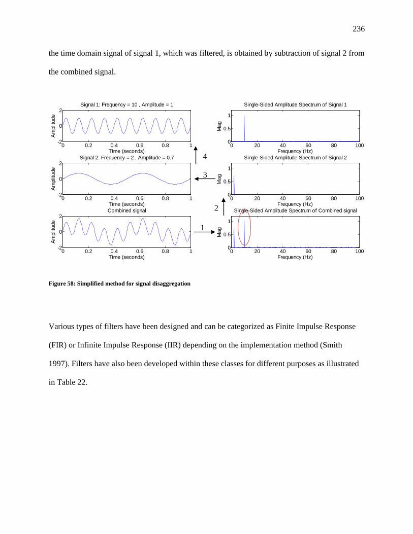
236

the time domain signal of signal 1, which was filtered, is obtained by subtraction of signal 2 from

the combined signal.

Figure 58: Simplified method for signal disaggregation

Various types of filters have been designed and can be categorized as Finite Impulse Response

(FIR) or Infinite Impulse Response (IIR) depending on the implementation method (Smith

1997). Filters have also been developed within these classes for different purposes as illustrated

in Table 22.

0 0.2 0.4 0.6 0.8 1-2

0

2Signal 1: Frequency = 10 , Amplitude = 1

Time (seconds)

Am

plitu

de

0 0.2 0.4 0.6 0.8 1-2

0

2Signal 2: Frequency = 2 , Amplitude = 0.7

Time (seconds)

Am

plitu

de

0 0.2 0.4 0.6 0.8 1-2

0

2Combined signal

Time (seconds)

Am

plitu

de

0 20 40 60 80 1000

0.5

1


Frequency (Hz)

Mag

0 20 40 60 80 1000

0.5

1


Frequency (Hz)

Mag

0 20 40 60 80 1000

0.5

1

Single-Sided Amplitude Spectrum of Combined signal

Frequency (Hz)

Mag 1

2

3

4

237

Table 22: Filter classification by type and purpose (Smith 1997)

Implementation method

FIR

(Convolution)

IIR

(Recursion)

Purpose

Time domain (smoothing, DC removal)

Moving average Single pole

Frequency domain (separating frequencies)

Windowed-sinc Chebyshev

Custom (Deconvolution)

FIR custom Iterative design

Four types of filters with different frequency response characteristics exist. These include: low-

pass, high-pass, band-pass, and band-reject filters (Smith 1997) with their functions implied in

their name. For example, a low-pass filter would remove high frequencies from a signal whereas

a band-reject filter would remove frequencies within a specific range. Filter design comprises

specification of frequency domain parameters to achieve a desired outcome. Design parameters

comprise: frequency response (low-pass, high-pass…), impulse response (IIR or FIR), design

method (Chebyshev, Windowed-sinc…), filter order, passband frequency, stopband frequency,

passband ripple, and stopband attenuation. These types of filter can be used in combination with

one another for specific applications. Figure 58 illustrates an example of a low pass filter and its

frequency response.

238

Figure 59: Example of filter frequency response

The passband corresponds to the range of frequencies that are passed through the filter whereas

the stopband refers to those that are rejected. The range of frequencies between the stopband and

the passband corresponds to the transition band; a ‘quick filter roll-off’ is characterized by a

narrow transition band (Smith 1997).

Chebyshev and Windowed-sinc filters can be used to separate signals in the frequency domain.

There are four types of Chebyshev filters, which are characterized by their ripple. Type 1 filters

allow frequency response ripple in the passband (exemplified in Figure 58), Type 2 filters have

ripple in the stopband, elliptic filters correspond to those with a ripple in both the stopband and

239

the passband, and Butterworth filters are described as maximally flat since the ripple corresponds

to 0% (Smith 1997). A comparison of these filters revealed that the Windowed-sinc had a better

stopband attenuation and increased flexibility but was much slower than the Chebyshev filter

(Smith 1997). The use of a Butterworth IIR filter was investigated because of its lack of ripple

and it was determined that the filtering capabilities were acceptable; thus this was the type

employed in the development of the disaggregation method.

The first step in designing the filter corresponded to determining the frequencies associated with

a specific electricity end-use. In the methodology proposed herein, this was achieved by

modeling the electricity consumption of a piece of equipment, based on its theoretical load

signature. Then an electricity signal corresponding to a particular use for a given duration was

derived by repetition of this cycle. Some loads can have several cycles during one day (i.e.

hoisting), while other end-uses in a mine may operate at a lower frequency (i.e. mine backfill

plants operating in batch mode at each shift). Thus it should be noted that modeled signal should

be sufficiently long to include 2 complete cycles for the activity to determine the periodicity of

electricity consumption from this end-use. Model parameters to account for operational

variability of the equipment were used to alter the individual cycles in the synthesized electricity

signal. Fourier transform algorithms are more efficient with signal lengths that correspond to an

integer power of 2 (Vetterling, Teukolsky et al. 1992) thus the length of the synthesized signal

was chosen to comprise a total of 128 samples.

The modeled consumption was then compared to periods of the actual aggregated time domain

electricity signal where the specific equipment was operational, and the variability parameters

were changed until the synthesized signal and the actual became comparable. Then FFT was

used to transform the synthesized time domain signal to the frequency domain, which allowed

240

the identification of the frequencies associated with this end-use activity. The resulting filter can

be said to be ‘smart’ because the specialist information contained within the model makes the

filter expectation guided.

The identified frequencies were used to design a filter to remove these frequencies from the

aggregated electricity signal, with the use of the designfilt function and the Filter Design &

Analysis Tool in MATLAB® (The MathWorks Inc. 2014). A graphical representation of the

filter frequency response superimposed on the frequency spectrum of the aggregated electricity

consumption permitted visual determination of whether adjustments to the filter design

parameters were necessary to remove / attenuate the frequencies of one specific end-use.

Next, an analysis was conducted to identify the periods in the aggregated time domain signal

where the specific end-use was in operation. This was achieved with the use of the Neural

Network Pattern Recognition procedure available in MATLAB®. A total of 48 periods of same

duration as those from the synthesized signal in the previous step were extracted from the

aggregated time domain signal, where the specific end-use to be filtered was operating in only

half of these periods. These segments were used as the input data to train the Neural Network to

identify the operating state of the specific end-use to be filtered. The output of the Neural

Network was used in a ‘sliding’ frame by frame analysis of the aggregated electricity signal to

classify each sampling interval based on the probability of operation of the specific end-use. The

frame duration in this analysis was the same as that used in the previous steps. For example,

Figure 59 shows a ‘sliding’ frame by frame analysis of a signal comprising a total of 20 samples,

each frame length is 10 samples and advances by one sample until the entire signal is analyzed. It

should be noted that in the actual case study the total number of samples corresponded to 40,320

and each frame comprised 128 samples.

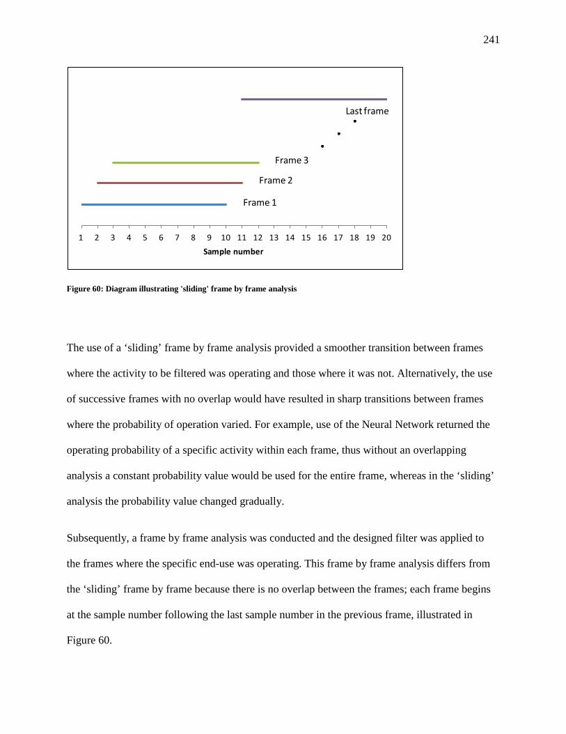
241

Figure 60: Diagram illustrating 'sliding' frame by frame analysis

The use of a ‘sliding’ frame by frame analysis provided a smoother transition between frames

where the activity to be filtered was operating and those where it was not. Alternatively, the use

of successive frames with no overlap would have resulted in sharp transitions between frames

where the probability of operation varied. For example, use of the Neural Network returned the

operating probability of a specific activity within each frame, thus without an overlapping

analysis a constant probability value would be used for the entire frame, whereas in the ‘sliding’

analysis the probability value changed gradually.

Subsequently, a frame by frame analysis was conducted and the designed filter was applied to

the frames where the specific end-use was operating. This frame by frame analysis differs from

the ‘sliding’ frame by frame because there is no overlap between the frames; each frame begins

at the sample number following the last sample number in the previous frame, illustrated in

Figure 60.

1 2 3 4 5 6 7 8 9 10 11 12 13 14 15 16 17 18 19 20Sample number

Frame 1

Frame 2

Frame 3

Last frame

242

Figure 61: Diagram illustrating a frame by frame analysis

It should be noted that the frame duration in this stage corresponded to the same length as those

in the previous steps to ensure that the spectra contained the same frequency bins to facilitate

comparison. In Fourier analysis the frequency resolution (𝛥𝑓 ) is determined as follows (Stanley

2005):

1. Calculate the period 𝑇 or the length of the signal (total sampling time)

𝑇 = 𝑁𝛥𝑡

where 𝑁 is the number of samples in the signal, and 𝛥𝑡 is the time interval between samples.

2. Calculate the frequency resolution 𝛥𝑓 (width of frequency bins)

𝛥𝑓 = 1𝑇

1 2 3 4 5 6 7 8 9 10 11 12 13 14 15 16 17 18 19 20Sample number

Frame 1

Frame 2

243

A signal with 𝑁 samples will have 𝑁/2+1 equally spaced frequency bins from 0 to 0.5*sampling

rate (Smith 1997), where the sampling rate corresponds to 1 𝛥𝑡� .Thus the frequency scale and

resolution of signals of different lengths will be different and the values for the frequency axis

may be different, which would impact spectral comparisons.

Windowing is a commonly used signal processing technique that removes the discontinuities

introduced from repetition of a finite signal by tapering the ends of the signal to zero (Smith

2008). A Hanning window can be used for such a purpose; this multiplies the start of a signal by

zero and the scaling factor gradually increases to 1 at the center of the signal, then decreases

gradually to zero at the end of the signal. This window is applied to frames of a signal where

these frames have a 50% overlap so that the sum of the corresponding samples in each frame

return the original signal (Boll 1979). The use of a window was not used in the methodology

proposed herein because the use of overlapping frames may have resulted in instances with

discrepancies between the overlapping samples in successive frames. This would occur where

the probability of operating state of an activity would transition from values greater than 50% to

lower than 50%, thus one frame would be filtered whereas the next one would not be filtered.

Furthermore, as there is no overlapping section at the start of the first frame and the end of the

last frame, this information would be discarded since it does not correspond to the original

signal. This may not be significant for high frequency activities (i.e. hoisting), but for low

frequency activities (i.e. batch mode backfilling) a larger proportion of information would be

lost.

Caution must be used during the filter application since the phase may be non-linear (Smith

1997), which could thus affect the information contained in the time domain by shifting the

244

signal along the time axis. This is important because information pertaining to the location of

events in a time domain signal is contained in the phase of its corresponding frequency domain

spectra (Smith 1997). In an energy management context, this outcome would not be suitable

because it is imperative to know when energy consumption occurs for implementation of: i)

optimized schedules to minimize electricity use during peak rate periods or ii) demand

management initiatives such as peak shaving or load shifting. This issue was mitigated with the

use of bidirectional filtering using the ‘filtfilt’ function in MATLAB which filters the filter

output in the opposite direction to counteract the filter delay (Widmann, Schroger et al. 2014).

The filtered signal comprised the aggregated electricity use from all remaining end-uses, thus

subtraction of the filtered signal from the original time domain signal provided a time domain

representation of the electricity consumption of the filtered end-use.

Electricity consumption from additional end-uses could be determined by iteration of the

aforementioned steps, where the total aggregated electricity signal would correspond to the

filtered time domain signal from the previous iteration. Figure 61 illustrates the steps from the

proposed top down methodology for disaggregation of an electricity signal.

245

Figure 62: Overview of proposed top down electricity disaggregation method

246

9.3 Isolation of the electricity consumption of a mine hoist from a mine’s total electricity meter data

The proposed top down methodology, described in the previous section, was applied to Garson

Mine, which is an underground mine owned and operated by Vale. This section will describe the

application of the ‘smart’ disaggregation methodology to extract the mine’s hoist electricity

consumption from the mine’s total electricity signal.

9.3.1 Establishing the minimum sampling interval

The first step consisted of determining the minimum sampling interval for the aggregated

electricity signal. The mine’s end-uses were categorized and the corresponding cycle time for

each of these was estimated for a 24 hour period, consisting of two 12 hour shifts per day,

illustrated in Table 23 prepared from data obtained from Mallett (2014). This information was

used to determine the minimum sampling frequency of the electricity signal required to satisfy

the Nyquist sampling theorem.

247

Table 23: Time and frequency of Garson Mine end-uses

End use Time/cycle (hours)

Time/cycle (minutes)

Time/cycle (seconds)

Frequency (Hz)

Main ventilation16

24

1,440 86,400 1.16E-05

Aux. ventilation 24 1,440 86,400 1.16E-05

Skip hoist 0.04 2.37 142 7.04E-03

Cage hoist 0.02 - 0.07 1.18 - 4.00 71 - 245 1.41E-02 - 4.08E-03

Paste plant 12 720 43,200 2.31E-05

Backfill plant 12 720 43,200 2.31E-05

Pumping 1 60 3,600 2.78E-04

Crushing 12 720 43,200 2.31E-05

Compressed air17 24 1,440 86,400 1.16E-05

Mining activities 12 720 43,200 2.31E-05

Surface facilities 12 720 43,200 2.31E-05

Table 23 shows that the end-use with the highest frequency corresponded to the cage hoist with a

cycle time of 71 seconds, which translated to 0.028 Hz. Thus the minimum sampling interval to

detect all end-uses at Garson Mine corresponded to 35 seconds. The sampling intervals for the

installed meters at the mine were 15 seconds and 15 minutes; therefore the use of the 15 second

interval meter data satisfied the Nyquist sampling theorem and was used in the disaggregation

method. 16 Ventilation is shown as a baseload but electricity use from ventilation systems in mines equipped with ventilation on demand would modulate to match the demand for fresh air 17 Compressors at this site are part of the baseload, but in mines where compressor supply exceeds demand and there is sufficient storage capacity electricity use would modulate. Modulation could also be indicative of a leak-free compressed air system.

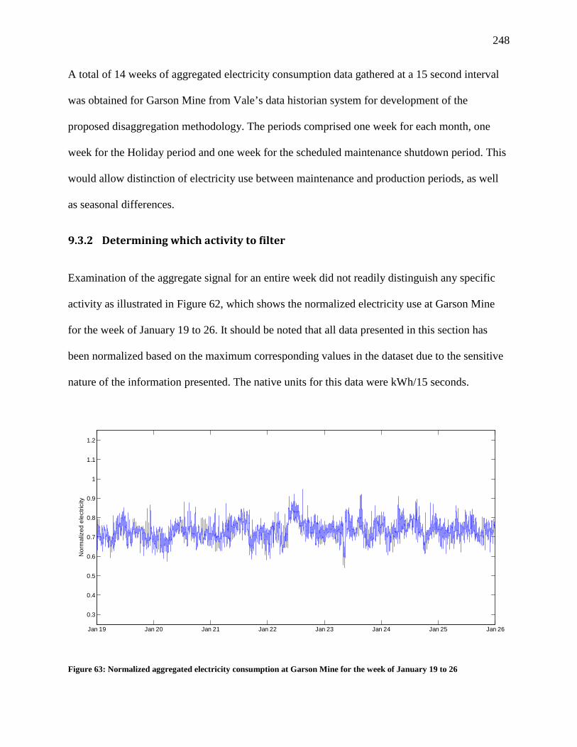
248

A total of 14 weeks of aggregated electricity consumption data gathered at a 15 second interval

was obtained for Garson Mine from Vale’s data historian system for development of the

proposed disaggregation methodology. The periods comprised one week for each month, one

week for the Holiday period and one week for the scheduled maintenance shutdown period. This

would allow distinction of electricity use between maintenance and production periods, as well

as seasonal differences.

9.3.2 Determining which activity to filter

Examination of the aggregate signal for an entire week did not readily distinguish any specific

activity as illustrated in Figure 62, which shows the normalized electricity use at Garson Mine

for the week of January 19 to 26. It should be noted that all data presented in this section has

been normalized based on the maximum corresponding values in the dataset due to the sensitive

nature of the information presented. The native units for this data were kWh/15 seconds.

Figure 63: Normalized aggregated electricity consumption at Garson Mine for the week of January 19 to 26

Jan 19 Jan 20 Jan 21 Jan 22 Jan 23 Jan 24 Jan 25 Jan 26

0.3

0.4

0.5

0.6

0.7

0.8

0.9

1

1.1

1.2

Nor

mal

ized

ele

ctric

ity

249

However, examination of data on a daily basis revealed that some intervals within this period

appeared to have greater variability than others, as exemplified in Figure 63 which shows the

data for January 21 and the coefficient of variance for 3 segments (standard deviation divided by

the mean).

Figure 64: Aggregate electricity consumption at Garson Mine for January 21

Examination of the electricity consumption for a 32 minute segment during these intervals

revealed a distinct pattern that was recognized as that corresponding to a repeating hoist cycle.

Figure 64 shows a 32 minute segment of the aggregate data for the week of January, comprising

128 samples, which corresponded to 10 hoist cycles, whereas Figure 65 shows the power versus

time diagram of one cycle from a cylindrical drum winder from (Walker 1988).

00:00 02:00 04:00 07:00 09:00 12:00 14:00 16:00 19:00 21:00 00:000.5

0.6

0.7

0.8

0.9

1

Nor

mal

ized

ele

ctric

ity (k

Wh)

CV=0.06 CV=0.04 CV=0.08

250

Figure 65: Segment of aggregate electricity use at Garson Mine for a 32 minute interval

Figure 66: Power / time diagram of cylindrical drum winder (Walker 1988)

0 5 10 15 20 25 30 350.5

0.6

0.7

0.8

0.9

1

Time (minutes)

Nor

mal

ized

ele

ctric

ity

251

Variations in the pattern shown in Figure 64 result from operational variability of the hoist due to

different: i) loading time, ii) unloading times, iii) payload weight and, iv) hoist speed. Further

variations may be due to electricity loads from other equipment starting and stopping at different

times within the hoist cycles.

The theoretical load signature curve for the Garson Mine hoist, parameterized from logged data

from the control system (Mallett 2014) was repeated for 10 cycles. During the braking stage of

the cycle, it was shown by the power curve in Walker (1988) and from the control system that

power can be generated; however since this regenerative power was not used at Garson Mine,

adjustments to the section of the curve corresponding to the braking stage were made. Then

interpolated values of the data sampled at 15 second intervals were determined and converted to

energy values. Figure 66 shows the normalized power and energy curves for 10 cycles.

252

The pattern illustrated in Figure 64 resembled that of the lower graph of Figure 66. Thus it was

hypothesized that the variability in the composite electricity consumption signal could be

attributed to the hoist.

This assumption was confirmed with external knowledge of the hoist operating schedule, which

at Garson Mine corresponded to operation between 3:00 PM and 7:00 AM to minimize

electricity use during peak rate periods (Mallett 2014). Figure 63 showed the aggregate

electricity consumption at Garson Mine for a 24 hour period which illustrates a different

consumption pattern during the period when the hoist operation may be curtailed.

Thus the hoist was selected as the first end-use to extract from the aggregate electricity signal at

Garson Mine. This selection was determined with the use of expert knowledge, such as the

generic load pattern of a hoist coupled with basic information on the operating schedule.

0 5 10 15 20 25 30 35-0.5

0

0.5

1

Time (minutes)

Nor

mal

ized

pow

er

0 5 10 15 20 25 30 35-0.5

0

0.5

1

Time (minutes)

Nor

mal

ized

ene

rgy

Figure 67: Hoist power and energy load signature curves for a 32 minute period

253

Removal of the hoist signal may facilitate subsequent identification of other end-uses that may

currently be ‘masked’ by the hoist electricity use.

9.3.3 Determination of probability of hoist operating state

Although the hoist at Garson Mine is scheduled to operate between 3:00PM and 7:00AM, there

may be some deviations to the schedule to meet production schedules. Identification of periods

when the hoist is operating may be readily discerned by examination of the aggregate signal but

this may be time consuming for large datasets. This task may be facilitated by defining criteria so

that a computer can be used. Thus the hoist operating state was determined with the use of the

Neural Pattern Recognition algorithm in MATLAB® (The MathWorks Inc. 2014) to identify the

sampling frames when the filter would be applied. The first step corresponded to the extraction

of four 32 minute segments for every week of data obtained, each comprising 128 points, where

the hoist was known to be operating in two of these segments and know not to be operating in

the other two periods. Then the frequency domain spectra of these segments were determined.

Figure 67 shows the signals and corresponding spectra for the extracted periods from the January

data. The extracted segments for the other periods are included in Appendix A.

254

0 5 10 15 20 25 30 350.5

0.6

0.7

0.8

0.9

Time (minutes)

Nor

mal

ized

ele

ctric

ity

0 0.1 0.2 0.3 0.4 0.5 0.6 0.7 0.8 0.9 10

0.05

0.1

Normalised frequency (π rads/sample)

Nor

mal

ized

mag

nitu

de

0 5 10 15 20 25 30 350.5

0.6

0.7

0.8

0.9

Time (minutes)

Nor

mal

ized

ele

ctric

ity

0 0.1 0.2 0.3 0.4 0.5 0.6 0.7 0.8 0.9 10

0.05

0.1


Nor

mal

ized

mag

nitu

de

0 5 10 15 20 25 30 350.5

0.6

0.7

0.8

0.9

Time (minutes)

Nor

mal

ized

ele

ctric

ity

0 0.1 0.2 0.3 0.4 0.5 0.6 0.7 0.8 0.9 10

0.05

0.1


Nor

mal

ized

mag

nitu

de

0 5 10 15 20 25 30 350.5

0.6

0.7

0.8

0.9

Time (minutes)

Nor

mal

ized

ele

ctric

ity

0 0.1 0.2 0.3 0.4 0.5 0.6 0.7 0.8 0.9 10

0.05

0.1


Nor

mal

ized

mag

nitu

de

Figure 68: Frames extracted from January data to train Neural Network

255

The magnitude values shown in the frequency spectra of the extracted periods were used as the

input values to train the Neural Network to detect whether the hoist was operating at a given

sampling interval. The 48 input samples were randomly divided to include 38 samples for the

Neural Network training stage, 5 samples for the validation, and 5 samples for testing. The

network was trained using scaled conjugate gradient backpropagation and the Network

Architecture comprised a total of three sigmoid hidden layers. Demuth et al (2008) provide more

details on the methodology employed. A so-called ‘confusion matrix’ plot shown in Figure 68

illustrates the types of errors encountered during the training stage (Demuth, Beale et al. 2008). It

can be seen that the Neural Network was 100% capable of determining the operating state of the

hoist from the blue cells in the bottom right corner of each matrix.

256

Figure 69: Neural Network confusion matrix

The output parameters from the trained Neural Network were then used to determine the

probability of the hoist operation for each sample of the signal for an entire week using a sliding

frame by frame analysis. Each frame comprised 128 samples, and the probability of hoist

operation corresponded to that of the sample in the center of the frame. Then the frame was

shifted forward in time by one sample and the probability of the next frame was determined. The

probability of hoist operation for the samples at the start and at the end of the sampling period

were assumed to correspond to those from the first and last points respectively that were

determined with the sliding frame by frame analysis. The results are illustrated in Figure 69. The

1 2

1

2

1950.0%

00.0%

100%0.0%

00.0%

1950.0%

100%0.0%

100%0.0%

100%0.0%

100%0.0%

Target Class

Out

put C

lass

Training Confusion Matrix

1 2

1

2

360.0%

00.0%

100%0.0%

00.0%

240.0%

100%0.0%

100%0.0%

100%0.0%

100%0.0%

Target Class

Out

put C

lass

Validation Confusion Matrix

1 2

1

2

240.0%

00.0%

100%0.0%

00.0%

360.0%

100%0.0%

100%0.0%

100%0.0%

100%0.0%

Target Class

Out

put C

lass

Test Confusion Matrix

1 2

1

2

2450.0%

00.0%

100%0.0%

00.0%

2450.0%

100%0.0%

100%0.0%

100%0.0%

100%0.0%

Target ClassO

utpu

t Cla

ss

All Confusion Matrix

257

blue line at the bottom of the figure corresponds to the aggregate electricity consumption for

Garson Mine for a one week period. The green line at the top of the figure shows the

corresponding probability of hoist operation for which the values are read on the axis on the

right. For example, a value of 1 indicates that the probability that the hoist was operating at that

time was 100% as determined by the trained Neural Network. Conversely, a value of 0 indicates

that the hoist was not operating, and the values between 0 and 1 correspond to probabilities

between 0 and 100% for the hoist operation. Hence a value of 0.5 would indicate a 50%

probability that the hoist was running.

258

Jan 19 Jan 20 Jan 21 Jan 22 Jan 23 Jan 24 Jan 25 Jan 260.25

0.5

0.75

1

Nor

mal

ized

tota

l ele

ctric

ity

Hoist electricity use estimate: 3.9161 % of total electricity


0

0.5

1

Pro

babi

lty o

f hoi

st ru

nnin

g

Figure 70: Aggregated electricity signal and probability of hoist operating for January 19 to 26

259

An estimate of the proportion of total electricity consumption was determined by counting the

number of 15 second sampling intervals where the probability of the hoist operating was greater

than 50%. Then this value was multiplied by the average electricity consumption per 15 second

interval determined from the synthesized hoist electricity load signature, which was presented in

Figure 66. The values obtained for the electricity consumption of the hoist from this estimate

were compared to those subsequently obtained with the use of a filter.

9.3.4 Designing the filter

Examination of the spectra derived from the frame samples of the synthesized hoist signal

indicated which frequencies were associated with the hoist electricity consumption. These were

compared to the corresponding spectra of segments of the aggregate electricity demand signal

illustrated in Figure 70. As there was variability in the patterns of the actual hoist cycles, three

segments of the aggregate data were randomly selected to ensure that the spectra of these signals

were comparable to that of the synthesized signal. It should be noted that the baseline of the

aggregate electricity signal was adjusted by subtracting a constant value from electricity data for

the entire period so that the minimum value in each frame would be zero. This was done to allow

superimposition of the synthesized hoist and actual electricity consumption signals to facilitate

comparison. Examination of the distinctions between the periods where the hoist was known to

be operating and those when the hoist was not operating used in the Neural Network training

provided further confirmation of the frequencies associated with the hoist. The top two spectra

on the right in Figure 67 and Appendix A show that peaks at frequencies corresponding to 0.16,

0.32, 0.48, 0.63, 0.79, and 0.95 π rad/sec were present when the hoist was operating.

260

Figure 71: Comparison of synthesized hoist and actual hoist signals

0 5 10 15 20 25 30 35-0.5

0

0.5

1

1.5

Time (minutes)

Nor

mal

ized

ene

rgy

0 0.1 0.2 0.3 0.4 0.5 0.6 0.7 0.8 0.9 10

0.5

1

1.5


Nor

mal

ized

mag

nitu

de

0 5 10 15 20 25 30 35-0.5

0

0.5

1

1.5

Time (minutes)

Nor

mal

ized

ene

rgy

0 0.1 0.2 0.3 0.4 0.5 0.6 0.7 0.8 0.9 10

0.5

1

1.5


Nor

mal

ized

mag

nitu

de

0 5 10 15 20 25 30 35-0.5

0

0.5

1

1.5

Time (minutes)

Nor

mal

ized

ene

rgy

0 0.1 0.2 0.3 0.4 0.5 0.6 0.7 0.8 0.9 10

0.5

1

1.5


Nor

mal

ized

mag

nitu

de

actual signalsynthesized signal



261

Examination of the spectra corresponding to the periods used to train the Neural Network where

the hoist was known not to be operating also revealed that there did not appear to be many

sizeable peaks at frequencies greater than 0.2 π rads/sec. It was decided that a lowpass filter

could be used to extract the hoist electricity consumption from the aggregated electricity signal

since those corresponding to the hoist were at the higher frequencies. The parameters used to

design the filter to remove the hoist frequencies from the aggregated signal are presented in

Table 24 and the filter frequency response is illustrated in Figure 71.

Table 24: Lowpass filter design parameters for extraction of hoist electricity consumption

Parameter Value

Response type Lowpass IIR

Method Butterworth

Passband frequency 0.1 π rads/sec

Stopband frequency 0.2 π rads/sec

Passband ripple 1 dB

Stopband attenuation 60 dB

Band to match exactly Stopband

262

0 0.1 0.2 0.3 0.4 0.5 0.6 0.7 0.8 0.9 1

0

0.2

0.4

0.6

0.8

1


Nor

mal

ized

mag

nitu

de

spectrumlowpassiir

Figure 72: Butterworth filter frequency response for Garson Mine hoist electricity extraction

263

It can be seen from Figure 71 that the magnitude values corresponding to the peak between 0.1

and 0.2 π rads/sample would not be completely removed by the filter designed with these

parameters. This was intentional since examination of the spectra in Figure 67 and Appendix A

showed that the magnitude values at these frequencies for the periods where the hoist was not

operating were not always zero. Thus an attempt was made to develop a filter that would

attenuate this peak but not completely eliminate it.

9.3.5 Applying the filter

The filter designed in the previous step was then applied to the aggregate electricity signal for

periods where the hoist was operating. First the signal was separated into frames each

comprising 128 samples. Then the probability of hoist operation was used to determine to which

frames the filter should be applied. A threshold value of 0.5 was applied in the frame by frame

analysis, whereby the filter was only applied to the frames where the combined probability of the

hoist operating for each point within that specific 32 minute period was greater than 50%. A

threshold value of 50% was chosen because this would provide a balance between application of

the filter to frames where the hoist was operational during a portion of the time. Use of a higher

value would have reduced the number of frames where the filter was applied, leaving more of the

hoist signal in the filtered signal. Conversely a lower threshold would have applied the filter to

more frames with partial hoist operation, thus attenuating some of the high frequencies that are

not associated to the hoist. Figure 72 illustrates the resulting filtered electricity signal from

Garson Mine after the filter was applied to frames where the probability of hoist operation was

greater than 50% to remove the hoist consumption from the aggregate signal. The original

aggregate signal is also included with both series were treated with the same normalization.

264


0.3

0.4

0.5

0.6

0.7

0.8

0.9

1

1.1

1.2

Nor

mal

ized

ele

ctric

ity (k

Wh)

original signalfiltered signal

Figure 73: Garson Mine electricity signal after hoist filter application overlaid on original aggregate electricity signal

265

It can be seen from Figure 72 that the variability associated with the hoist electricity

consumption was reduced after application of the filter. A comparison of sections of the signal in

Figure 72 where the filter was applied with other frames that remained unfiltered shows that

there does not appear to be much difference between the filtered and unfiltered sections of the

signal. The difference between the filtered and unfiltered frames could be quantified by

comparison of their spectra. However, examination of one daily segment of the filtered signal

revealed that the filtered frames appear to have less noise, which corresponded to the removal of

the high frequencies during the filtering stage of the methodology. Figure 73 shows the filtered

signal for January 22nd

, where the first part of the signal was filtered and the center was not

filtered for the hoist extraction.

266

Figure 74: Electricity signal at Garson Mine after hoist filter application for January 22

Jan 22 Jan 230.5

0.55

0.6

0.65

0.7

0.75

0.8

0.85

0.9

0.95

1N

orm

aliz

ed e

lect

ricity

(kW

h)

Filtered frames

Unfiltered frames

267

It can be seen by comparison of the filtered frame with unfiltered frame from Figure 73 that the

use of a lowpass filter may have removed too much of the high frequency components from the

aggregate signal. This may be rectified by:

i) means of adjustments to the filter design parameters such as with the use of a custom

bandstop filter to attenuate specific frequency components,

ii) or use of a different signal processing technique such as spectral subtraction which is

employed to remove noise from audio signals.

Use of a more selective method to filter the hoist from the aggregate signal may improve the

disaggregation method.

9.3.6 Determination of hoist electricity consumption

The hoist electricity consumption signal was then derived by subtraction of the filtered signal

from the original aggregate signal. The resulting hoist electricity consumption signal is

illustrated in Figure 74 along with the probability of the hoist operating state. Figure 75 shows a

32 minute segment of the hoist electricity consumption signal extracted from the aggregate

signal. It can be seen from the load signature shown in Figure 75 that the applied filter has

appeared to have successfully extracted the hoist electricity consumption from the aggregate

signal because the load signature resembled that of the synthesized hoist signal in Figure 66. This

could be quantified by comparison of the spectra for the extracted period with that of the

synthesized hoist.

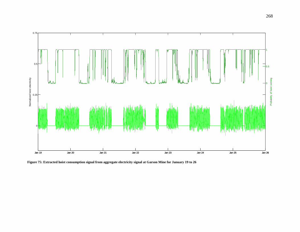
268

Figure 75: Extracted hoist consumption signal from aggregate electricity signal at Garson Mine for January 19 to 26


0

0.25

0.5

0.75N

orm

aliz

ed h

oist

ele

ctric

ity


0

0.5

1

Pro

babi

lty o

f hoi

st ru

nnin

g

269

Figure 76: Extracted hoist signal from aggregate electricity signal at Garson Mine (32 minute segment)

0 5 10 15 20 25 30 35-0.05

0

0.05

0.1

0.15

0.2N

orm

aliz

ed h

oist

ele

ctric

ity

Time (minutes)

270

The total electricity use from the hoist for the week of January 19 to 26 was then calculated by

summing the electricity use from the hoist for each 15 second interval within this period, which

allowed determination of the proportion of total electricity use attributable the hoist.

While the methodological development was exercised using January data, the disaggregation

methodology was applied to all other periods of aggregated electricity consumption data that was

provided for this study. A summary of the results is presented in Table 25, and Appendix B

presents an overview of the analysis for each period.

271

Table 25: Proportion of total electricity used by the hoist at Garson Mine for various periods

Period Hoist electricity consumption estimate (% of total)

From average consumption18 From filtered signal

January 3.92 4.13

February 3.54 3.55

March 3.75 3.86

April 3.91 3.98

May 2.15 2.20

June 3.88 3.96

July 2.68 2.80

August 2.44 2.43

September 3.00 3.04

October 3.40 3.47

November 3.42 3.46

December 2.66 2.73

Holidays 2.14 2.22

Shutdown 0.18 0.10

Average of 12 months19 3.23 3.30

The results presented in Table 25 show that both methods used for estimation of the proportion

of total electricity from the hoist provided similar values but those derived from counting the

number of 15 second intervals where the probability of the hoist operation was greater than 50%

yielded slightly lower results for the weeks excluding Holidays and Shutdown periods.

An energy audit conducted at Garson Mine established that the proportion of electricity

consumed by the hoist corresponded to 3.41 % of total electricity (Mallett 2014), thus this

18 The values in this column were estimated by multiplication of the number of 15 second intervals where the probability of hoist operation was greater than 50% with the average hoist electricity consumption from the synthesized hoist signal. 19 Excluded Holidays and Shutdown periods

272

provides confidence in the values determined by the disaggregation method developed as part of

this work.

9.3.7 Issues with the proposed disaggregation methodology and suggested future

refinements

It was assumed that the discrepancies between both methods used to estimate the electricity use

from the hoist could be due to the use of the average hoist cycle electricity consumption value

derived from the synthesized load curve for 10 cycles. The energy use from the hoist would vary

based on the amount of material being lifted, thus a refined average electricity consumption

value that considered the mass of material could provide results between both methods that

would be more similar. Alternatively, it is possible that the filter removed data from frequencies

that did not belong to the hoist, and thus overestimated the electricity consumption from this end-

use. This may be due to the application of a lowpass filter or due to the filtering of frames with

partial or intermittent hoist operation.

Examination of the extracted hoist signal from all the assessed periods showed that although

regenerated power was not used at Garson Mine, there were some negative electricity

consumption values. This was because for some intervals the values from the filtered signal were

greater than those from the original aggregate signal. It is estimated that this was because

application of the filter did not remove the average consumption of the hoist from the aggregated

signal when producing the filtered signal, thus the average consumption derived from the

synthesized hoist signal was subtracted from the filtered signal. This can be explained with the

use of the diagram in Figure 76 which shows that the DC component (first peak in the spectra

which corresponds to the average value of the time domain signal) remained unchanged in the

273

filtered signal because it was multiplied by 1. Since the filter was designed to remove the

electricity consumption of the hoist from the aggregate signal, the average hoist cycle

consumption derived from the synthesized hoist signal was subtracted from each of the frames

where the filter was applied to obtain the filtered signal.

Figure 77: Butterworth frequency response for Garson Mine hoist electricity extraction

The cage hoist at Garson Mine is used to transport workers and supplies underground to and

from four levels of different depths. The total time required for one cycle to the shallowest level

corresponded to 71 seconds whereas the time to the deepest level was 245 seconds. Examination

of the daily cage hoist schedule revealed that 93% of the 29 trips were to the deeper levels, and

that the time interval between trips was not constant. Thus the load signature of the individual

cycles would be different and the daily pattern for the cage hoist electricity consumption would

not be periodic. Knowledge of the cage hoist schedule and the various load signatures would be

0 0.1 0.2 0.3 0.4 0.5 0.6 0.7 0.8 0.9 10

0.2

0.4

0.6

0.8

1


Nor

mal

ized

mag

nitu

de

spectrumlowpassiir

DC peak (represents average of signal)

Filter frequency response (DC remains unchanged in filtered signal)

274

required in the disaggregation method, however it may be difficult to discern between the cage

and the skip hoist due to their similar load signatures.

Comparison of the filtered signal for all the periods assessed during this study revealed that there

were similar patterns that repeated in the different weeks. All of the periods began on a Saturday

and ended on a Friday, therefore some activities seemed to occur at the same time every week.

Thus discussions with mining personnel may provide clues to assist in the identification of these

activities for subsequent iterations of the disaggregation methodology. Examination of periods

with lower electricity use such as the scheduled maintenance shutdown period may be useful to

identify the load signature of some equipment because of the reduced number of operating

equipment.

The use of regenerated power during the braking stage of the hoist cycle was investigated and it

was estimated that the potential electricity savings would correspond to roughly 6.7% of the

electricity consumed by the hoist. However, since this activity only accounted for about 3% of

total electricity use at the mine, this would only translate to total electricity savings of 0.2%.

Thus the savings potential from this measure may be considered negligible. Furthermore,

periodic regeneration of electricity for short durations may cause issues in the electrical system at

the mine, which may be overcome by storing the regenerated electricity but this would increase

the investment for this potential energy conservation measure.

The analysis presented in this chapter indicated that an electricity signal from a mine could be

disaggregated to extract the electricity use from the hoist. This was achieved with the use of

information from both the time and frequency domains, combined with expert knowledge of

electricity load signature and operating schedule for the hoist.

275

Recursive application of the methodology developed during this study could be used to estimate

the electricity consumption of other end-uses, where the aggregate signal would correspond to

the filtered signal of the previous iteration. It is anticipated, with knowledge of the operating

schedule of the remaining end-uses from Table 23, that the next end-use extracted for Garson

Mine may correspond to pumping. The disaggregation methodology for this activity would have

to consider the storage capacity, flowrates from groundwater, precipitation, and control measures

used to activate the pumps to derive the load signature. Thus the next iteration may be more

challenging than the hoist extraction.

Although some issues have been identified with the methodology developed during this study,

refinements with additional work could address these shortcomings. Future research should

investigate enhancement of the filter design parameters or the use of spectral subtraction to

reduce or eliminate the misallocation of frequencies to various end-uses. Nonetheless, a

disaggregation methodology was developed during this work that could be applied to estimate

the electricity use of a hoist in an underground mine and subsequent reiterations could estimate

other end-use electricity consumption.

276

10 Improved energy audit and data interpretation and their impact on

production patterns and profitability

10.1 Introduction

With milling costs representing 43 to 45% of total costs for a mining operation (Curry, Ismay et

al. 2014), mills present an excellent opportunity for managing expenditures within the mining

sector. It was also reported that in a mineral processing plant, comminution energy consumption

may correspond to as much as 60% of total energy (Sayadi, Khalesi et al. 2014), which provides

incentive to improve efficiencies in these plants. As efficiencies for comminution processes

correspond to 1-2% and grinding at 2-3% (Sadrai, Meech et al. 2011), there appears to be

significant room for improvement. Methods for improving efficiencies in milling have been

investigated and a summary illustrating the various research areas was presented in Curry et al

(2014). These included: pre-concentration, more efficient grinding technologies, and coarse

particle separation.

In 2008, an energy audit was conducted at Vale’s Clarabelle Mill by Byron Landry & Associates

in order to identify potential energy savings (Landry 2009), precipitated by rising energy costs

and market conditions. A review of this work was undertaken to gain a better understanding of

energy use in mineral processing facilities and to determine whether additional energy and cost

savings existed at Clarabelle Mill. Furthermore, an analysis was conducted for the 2012 census

year to determine potential cost savings that could arise due to a revised Ontario billing rate

structure, implemented in 2011. The analysis was also extended to other metal ore milling

facilities operating in Ontario to determine the possible savings that could be achieved across the

industry.

277

10.2 Clarabelle Mill flowsheet and process description

Clarabelle Mill has been in operation since 1971 (Pickett, Hall et al. 1978) and processes ore

from various Vale and QuadraFNX mines (now KGHM International) (Barrette, Taylor et al.

2012). Flowsheet design and modifications have been described in various books, journal and

conference publications (Pickett, Hall et al. 1978, Tenbergen, Throssell 1989, Damjanovic,

Goode et al. 2000, Xu, Wilson 2000, Kerr, Bouchard et al. 2003, Doucet, Price et al. 2010,

Barrette, Taylor et al. 2012). The process flowsheet in place at the time of the 2008 energy audit

consisted of a comminution stage followed by a flotation circuit.

A simplified illustration of the comminution circuit, produced from the aforementioned sources,

is presented in Figure 77 whereas the flotation circuit is illustrated in Figure 78.

278

Figure 78: Comminution circuit flowsheet in 2008

Magnetic Separation

Ball Mills (5 x 1492 kW)

Rod Mills (2 x 1492 kW)

Shorthead Crushers (4 x 223 kW)

Standard Crushers (4 x 223 kW) SAG Mill

(8206 kW)

Crushed Ore

279

Figure 79: Flotation circuit flowsheet in 2008 (Lawson, Xu 2011)

The comminution stage comprised two routes: a SAG mill circuit, and a crushing and grinding

circuit, controlled by an Expert Grinding Control System. Throughput was maximized through

the SAG circuit, which can process half of the ore based on total mill design capacity. When

throughput exceeded the SAG capacity, ore was processed via the alternate crushing and

grinding circuit. The crushing and grinding is performed by four lines of standard and shorthead

crushers followed by two rod mills (Damjanovic, Goode et al. 2000, Kerr, Bouchard et al. 2003).

Subsequently, the ore from both circuits is fed to five ball mills, which are equipped with

cyclones, where the cyclone overflow is pumped to the magnetic separation stage of the mill.

Cu Clnr

Sulphide Tails

Bulk concentrate

Non-sulphide tails

A Rougher B Rougher Scavenger

MAG-RCLNR

B Cleaner

Cu Rougher Cu Scavenger

Cu concentrate

Scav Cleaner

Ball Mill (750 kW)

Ball Mill (1500 kW)

Non-magnetic Magnetic

Magnetic Separation

Ball Mills (2 x 1500 kW)

MAG-CLNR

280

Once the magnetic and non-magnetic fractions are divided, various flotation circuits further

separate the minerals from the waste. The result is the production of a copper concentrate which

is sold to market and a bulk nickel concentrate which is fed to a smelter for further refining

(Lawson, Xu 2011).

Lawson (2011) stated that after 2008, the ball mills were removed from the non-magnetic

flotation stages; the 1500 kW ball mill was moved to the comminution circuit whereas the 750

kW ball mill was damaged and thus retired from operation. Although the flowsheets between

2008 and 2012 differed, the equipment used at the facility was the same with the exception of the

750 kW ball mill in the latter year. It is estimated that the impact of this difference is negligible

for the purpose of the energy analysis because the retired ball mill demand corresponded to less

than 5% of the plant total demand.

10.3 Electricity audit

10.3.1 Review of past audit

In 2008, a significant amount of effort was applied from Landry and Vale personnel to collect

the data for the Clarabelle Mill audit. The dataset consisted of historical values retrieved from the

company’s PI system, which allowed calculation of electricity use for each piece of equipment,

on an hourly basis for the entire year. The data was organized into 12 equipment categories

which included: SAG mill, Ball mills, Rod mills, Crushers, Agitators, Pumps, Blowers,

Compressors, Fans, Conveyors, Heat trace, and Misc. process. The collated values consisted of:

energy (kWh), current (Amps) or run time (hours). Subsequently, the non-energy data was

converted to energy units and the hourly values were summed to obtain annual consumption for

each piece of equipment.

281

Detailed data analysis ensued, as part of the energy audit process, to examine areas for potential

savings. The following ten opportunities for reducing electricity consumption at the plant by 5%

were identified, with payback periods ranging from zero to nine years (Landry 2009):

• Optimize blower operating sequence to maximize use of more efficient units

• Minimize idling of conveyors

• Utilize process control measures on main sumps

• Refine SAG mill process control system

• Reduce compressed air leaks

• Implement motor rewind and replacement strategy

• Optimize amount of water use in the crushing section of the plant

• Replace existing light fixtures with more efficient units

• Exploit energy in tailings pond discharge with installation of micro-hydro turbine

• Replace fluid coupling pump drives with more efficient variable frequency drives

All of the aforementioned measures were considered as good candidates from an energy

management standpoint, where implementation could deliver electricity savings. Subsequently, a

review of the audit was conducted to gain a better understanding of how electricity is consumed

in a mineral processing facility and to possibly identify additional energy savings.

10.3.2 Converting collected data into energy values

Some of the data gathered during the electricity audit of the plant consisted of hourly electricity

consumption that could be summed to obtain the annual consumption. Specifically, 72% of the

electricity consumption data was allocated in this manner. This indicates that there is minimal

282

uncertainty for most of the data in the audit since no assumptions or calculations were required

for this portion of the data.

Conversely, for other pieces of equipment, the hourly kWh consumption data was not available

therefore conversions were employed to calculate the annual electricity consumption for the

equipment in question.

For some equipment, current (Amps) values were recorded on an hourly basis which were

converted to hourly energy (kWh) values using voltage, power factor and operating hours

following the equations from Capehart et al (2012 p.268-269) for single-phase and three-phase

motors. The proportion of electricity use that was calculated from the conversion of current to

energy corresponded to 18.4% of total electricity data.

Power factor values vary depending on the rated capacity and load of a motor and can either be

leading or lagging. It should be noted that facility power factor values are not the same as those

of the individual equipment and that the individual power factor values should be used when

available. Synchronous motors provide power factor correction to the facility (Thumann, Mehta

2008) and since large motors of this type were in use at Clarabelle Mill, a conservative value of

0.85 for the facility was used in this audit due to the lack of individual values.

Where run time data was gathered, voltage, current and power factor estimates were used to

calculate the annual energy consumption for single-phase and three-phase motors as per

Capehart et al (2012 p.268-269). The proportion of total electricity that was calculated from run

time data corresponded to 6%.

283

For some equipment no hourly data was collected; this included 43 pumps where an annual use

factor of 75% was estimated, which corresponded well with the average annual use of other

pumps. Calculation of the electricity consumption for these pumps (corresponding to 17% of

total electricity consumed by all pumps, or 3.6% of total electricity consumption) was achieved

by using the rated capacity and an estimate for the voltage were used to calculate a value for the

current. Then using these estimates and the power factor value, corresponding to that assumed

for the other equipment, in the equations from Capehart et al (2012 p.268-269) permitted to

estimate the electricity consumption from these pumps.

10.3.3 Applying a top-down / bottom-up approach

Up to this point the analysis consisted of a bottom-up approach, where energy consumption from

individual components was summed to estimate the total annual electricity consumption at

Clarabelle Mill. Comparison of this amount to the actual total electricity supplied to the facility

(top-down component) indicated that 8.8% of total electricity was unallocated, which left

uncertainty. This variance was deemed significant and so precipitated a more detailed review in

order to allocate this portion of electricity within the milling operation to gain full understanding

of how electricity is consumed at the plant. An energy balance ensures that allocated energy

consumption is not over or underestimated and allows validation of assumptions made within the

bottom-up approach. The use of a top-down / bottom-up methodology provides an opportunity

for reconciliation and increases confidence in the values and the results obtained during an

energy audit.

Table 26 presents solutions to issues identified with the bottom-up audit during the data

reconciliation process. For example, during the original audit some of the equipment at the mill

284

was omitted, which is listed in Table 27. Table 28 shows the corrected and final electricity

allocation to each equipment category, including allocation to excluded equipment in the original

audit.

285

Table 26: Data reconciliation issues and solutions

Issue Solution

Missing or

corrupt data for

certain periods

It was determined whether the equipment was running during these periods by

examining the throughput data. If the equipment was in use, a use factor

(number of missing values/number of collected values) was used to prorate the

annual electricity consumption for a complete year.

Assumed

current and

voltage values

The available equipment rating (kW) from the inventory list was examined for

agitators, pumps, blowers, compressors, fans, conveyors, heat trace, and misc.

process equipment to confirm that the estimated current, voltage and power

factor values used in the assessment were acceptable. In some instances the

calculated demand values (kWh/h) exceeded the rated capacity (kW) therefore

the assumed current (Amps) values were replaced with values calculated from

the equipment power rating using the equations from Thumann and Mehta

(2008 p.62). For one of the pumps where hourly current data was provided and

thus was not altered, the average annual load (kWh/h) exceeded the rated

capacity (kW) of the pump therefore the assumed voltage value was reduced to

the next highest voltage supplied to the facility. The result of the modified

current and voltage values was that the average load was less than the rated

capacity. This represents a potential source of error or uncertainty therefore it

was recommended that these parameters should be measured.

Use of facility

power factor

The power factor for a facility varies when inductive and capacity loads are

turned on or off, thus using a constant facility power factor for individual

equipment represents a source of uncertainty where it is used to calculate

electricity consumption. Measurement of the power factor for each piece of

equipment would provide a more accurate representation of the bottom-up

electricity consumption values calculated during the audit. Use of the average

facility power factor value may over- or under-estimate the electricity

consumption of the individual pieces of equipment. During this audit, 26% of

the electricity use at the facility was calculated using the average plant power

factor value.

286

Omission of

equipment

categories

It was observed that lighting was not included in the allocated electricity

consumption. Therefore the lighting consumption was allocated based on a

cursory survey presented in section 3.9 of Landry (2009). The lighting audit

was conducted in areas of the plant that were easily accessible therefore not all

lights were included, thus this represents a possible source of error.

Omission of

individual

equipment

The final stage in the reconciliation step consisted of a comparison of the

equipment inventory and the equipment for which electricity was allocated. It

revealed a total of 80 items of various types, representing a total rating of

5,706 kW, that were not included in the original audit. Table 27shows a

summary of the excluded equipment. The remaining unallocated electricity

consumption, after corrections were applied as described in this section, was

distributed to the various equipment categories based on the % of total kW

excluded values from Table 27. For example, 71% of the total unallocated

electricity consumption was allocated to the pumps category.

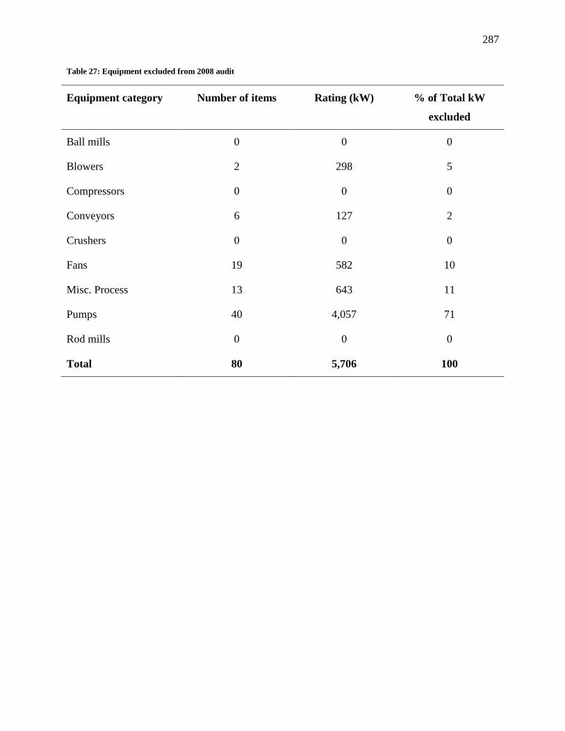
287

Table 27: Equipment excluded from 2008 audit

Equipment category Number of items Rating (kW) % of Total kW

excluded

Ball mills 0 0 0

Blowers 2 298 5

Compressors 0 0 0

Conveyors 6 127 2

Crushers 0 0 0

Fans 19 582 10

Misc. Process 13 643 11

Pumps 40 4,057 71

Rod mills 0 0 0

Total 80 5,706 100

288

Table 28: Electricity allocation and reconciliation summary20

Electricity

consumption

(Landry 2009)

Corrected

electricity

consumption

Unallocated

consumption

Final electricity

consumption

Equipment

Category

% Accounted

SAG 21.4 24.0 24.0

Rod Mills 6.6 7.0 7.0

Ball Mills 32.4 34.7 34.7

Crushers 1.7 0.8 0.8

Agitators 0.8 0.9 0.9

Pumps 20.4 19.8 3.2 22.9

Blowers 1.5 1.6 0.2 1.8

Compressors 1.1 1.1 1.1

Fans 0.7 0.6 0.5 1.0

Conveyors 3.8 4.2 0.1 4.3

Heat trace 0.1 0.1 0.1

Misc. Process 0.6 0.7 0.5 1.2

Sub-total 91.2 95.2 4.4 99.7

Lighting 0.3 0.3

Sub-total 95.6 100.0

Unallocated 8.8 4.4 0.0

Total 100.0 100.0 100.0

20 Total may not match the sum of individual values due to rounding

289

It can be observed from Table 28 that the corrections made to the calculations to allocate the

electricity consumption to the various equipment categories did not produce significant changes

to the percent allocation of each equipment category however the sum of these minor changes

resulted in reducing the unallocated electricity from 8.8% to 4.4%. An investigation of excluded

equipment from the audit allowed distribution of the unallocated electricity to its respective

categories, which resulted in complete allocation of all electricity supplied to the mill.

Although the material covered in this section may seem pedestrian or of routine detail, it is

important to understand the practice of energy management in addition to the theory; this is the

level of scrutiny and attention to detail that is required for a thorough and reliable energy

assessment. Using only the top-down approach does not provide a full understanding of energy

use at a facility. Conversely, the bottom-up method used on its own does not instill confidence in

the energy audit values because of the lack of reconciliation; assumed values could be incorrect,

and / or data may be missing. The use of both methods together provides more accurate audit

values which in turn increases confidence in estimated savings from proposed energy

conservation measures. The top-down / bottom-up methodology may be used as part of a

continuous improvement process such as that found in the ISO 50001 energy management

standard (International Organization for Standardization 2011b).

10.3.4 Energy analysis

An understanding of energy use is important to identify areas where efforts should be focused for

savings. Sankey diagrams are useful to show how energy is used in a process plant since the

widths of the bands are proportional to the amounts of energy they represent. A Sankey diagram

290

was created to illustrate the energy flows at Clarabelle Mill using the audited 2008 annual

electricity data, and is shown in Figure 79.

Figure 80: Clarabelle Mill Sankey diagram for 2008

It can be observed that the processes consuming the most energy comprise the SAG mill, ball

mills and pumps which correspond to areas which may provide opportunities to reduce energy

consumption with further investigation.

10.3.5 Part-load efficiency curve

An understanding of the variables that affect demand and energy consumption is essential in

energy management to benchmark and improve efficiency. In advance of the audit, it was known

that operation of equipment at part-load conditions can have a negative effect on energy

efficiency (Doty, Turner 2009) which in mineral processing operations can be the result of

291

changes in throughput. An investigation of the influence of throughput on demand and energy

consumption ensued to investigate the correlation. The throughput was examined in terms of %

design capacity, which corresponded to the percentage of tonnes of ore processed on an hourly

basis with respect to the plant’s hourly design capacity.

A model relating the average hourly demand (MWh/h) and hourly throughput (% design

capacity) for 2008 is presented in Figure 80. The upper and lower 95% confidence intervals were

calculated following the procedure outlined in Brown (2001). It should be noted that throughput

below 5% of design capacity was excluded from the analysis; these instances mostly

corresponded to the scheduled maintenance shutdown period. Furthermore, the hourly demand

values were normalized against the maximum value due to the sensitivity of the information

presented.

Figure 81: Normalized average hourly electricity demand versus throughput expressed as % design capacity

R² = 0.73

0

0

0

1

1

1

1

1

0.0

0.2

0.4

0.6

0.8

1.0

1.2

1.4

0 10 20 30 40 50 60 70 80 90 100 110 120 130

Nor

mal

ized

Ave

rage

hou

rly e

lect

ricity

dem

and

Throughput (% design capacity)

2008 hourly Upper Limit (95% confidence) Lower Limit (95% confidence)Average Combined circuits SAG circuit

292

It can be observed from Figure 80 that electricity demand increases with throughput and that the

relation between these variables is not linear. There is also greater variability in demand at lower

throughput, illustrated by the error bars for the average of each % design capacity interval. It can

also be observed that there are two distinct clusters of the hourly data, disjoint at around 50%

design capacity. It is presumed that the data at the lower range represented the use of the SAG

mill circuit alone, whereas the data at throughput values greater than 50% design capacity

corresponded to the parallel operation of both the SAG, and crushing and grinding circuits. For

the purpose of this study, the composite curve represented by all data was used.

A model for specific energy consumption was produced using the modeled MWh/h and hourly

throughput expressed as % design capacity and is presented in Figure 81.The specific energy

consumption data was normalized against the model value at 100% design capacity due to the

sensitive nature of the information. The inset in Figure 81 shows the monthly and annually

aggregated data from 2008 and 2012 with the part-load model and confidence limits derived

from hourly data. The correlation between the hourly model and the monthly and annual data

illustrate that a part-load analysis can be undertaken at facilities where hourly data is not

available.

293

Figure 82: Normalized specific energy consumption versus throughput expressed as % design capacity (hourly, monthly and annual data)

It can be observed from Figure 81 that at low throughput, the specific energy consumption

increased rapidly which is consistent with prior understanding of part-load electricity

consumption. Furthermore, operation of the mill at design capacity is the most efficient in terms

of electricity consumption per tonne of ore milled.

10.4 Potential energy conservation at Clarabelle Mill

Energy savings opportunities were investigated using the models and information from Figure 80

and Figure 81. The investigation focused on the potential savings which could arise by

modifying the existing schedule so that the facility operated at 100% of design capacity, while

maintaining the original monthly and annual production. Practically, this corresponds to altering

shift operating patterns and was motivated by noting that this rate of production corresponded to

the lowest energy consumption per tonne of ore. Although specific energy consumption was

0.0

0.1

0.2

0.3

0.4

0.5

0.6

0.7

0.8

0.9

1.0

0 10 20 30 40 50 60 70 80 90 100 110 120 130

Nor

mal

ized

Spec

ific e

nerg

y


2008 hourly Upper Limit (95% confidence) Lower Limit (95% confidence) Modeled kWh/tonne

0.0

0.1

0.2

0.3

0.4

0.5

0.6

0.7

0.8

0.9

1.0

0 10 20 30 40 50 60 70 80 90 100 110 120 130

Nor

mal

ized

Spec

ific

ener

gy


Upper Limit (95% confidence)Lower Limit (95% confidence)2008 Monthly2012 Monthly2008 Annual2012 AnnualModeled kWh/tonne (from hourly data)

294

lower at throughputs greater than 100%, these points were not selected as the target as it was

unknown if these production rates could be sustained. To take advantage of time-of-use rates

(TOU), operating time was maximized during off-peak electricity periods, which occurred on

weekends as well as weekdays from 7PM to 7AM. Although these circumstances are specific to

Clarabelle Mill, such considerations feature in many jurisdictions and so there is no great loss of

generality. The remaining hours necessary to meet actual production were scheduled during on-

peak hours. The analysis was conducted on a monthly basis to provide schedule flexibility,

which was also useful since 2012 monthly electricity data was available and thus allowed a

comparison of the 2008 and 2012 results. Implementation of a daily intermittent schedule may

not be practical or technically feasible but would offer the most electricity cost savings by taking

advantage of TOU rates. Alternatively, a weekly intermittent schedule would also deliver savings

with respect to electricity consumption per tonne of ore milled.

It should also be noted that during consideration of these revisions to the operating schedule, a

base load of 10% of total electricity consumption was included during periods of no production

to account for equipment that must operate regardless of production. These could include

ventilation systems, agitators and heat trace, among others. Investigation of the electricity data

from the energy balance in Figure 79 revealed that consumption of all mills and crushers

corresponded to 67% of total electricity at Clarabelle Mill. The remaining 33% of electricity was

consumed by pumps, fans, blowers and agitators among other types of equipment. Assuming that

all agitators, blowers, fans, heat trace, misc. process and lights remain in operation during

periods of no production this would only correspond to 5% of total electricity but a base load

estimate of 10% was applied during the analysis. This reflects the fact that some of the pumps

295

and conveyors of the plant could be running during periods of no production. A summary of the

2008 annual results are presented in Table 29.

Table 29: Potential savings from optimized TOU schedule and throughput - 2008 analysis

Actual Optimal Point

Upper Limit

(95%

confidence)

Lower Limit

(95%

confidence)

Average throughput

(% design capacity)

74 100 100 100

Savings vs actual

(kWh/tonne)

-- 14% 1% 26%

It can be observed from Table 29 that 1%, 14% and 26% savings could be achieved for operation

at minimum specific energy consumption at the upper limit, optimal and lower limit respectively.

Subsequently the analysis was repeated with 2012 monthly data. It should be noted that February

and September of 2012 had low production due to operating challenges and maintenance

shutdown respectively, therefore these months were excluded from the analysis. Table 30 shows

the results from the optimized schedule and lower specific energy consumption.

296

Table 30: Potential savings from optimized TOU schedule and throughput – 2012 monthly analysis

Actual Optimal Point

Upper Limit

(95%

confidence)

Lower Limit

(95%

confidence)

Average throughput

(% design capacity)

47 100 100 100

Savings vs actual

(kWh/tonne)

-- 36% 27% 45%

Table 30 shows that in 2012 if Clarabelle Mill had been operated at 100% of design capacity at

all times when operating, the recorded annual production could have been achieved by operating

an average of 11 hours per day which could all be scheduled during off-peak electricity rate

hours. The potential savings resulting from this scenario ranged from 36-45%; undoubtedly

investigation of the feasibility of implementing this option would be valuable. Although the

reasons for which throughput at the mill during these years was lower than design capacity are

unknown, market conditions, operational challenges, unplanned maintenance and reduced ore

supply from mines could be possible explanations.

10.5 Demand charges in Ontario via 5CP billing

Electricity prices in Ontario vary based on supply and demand; the Independent Electricity

Supply Operator (IESO) manages bids from generators to supply electricity as well as offers

from consumers to reduce consumption in order to meet the forecast demand at the lowest

available price (IESO 2013d). Subsequently, as demand increases so does the price of electricity

(IESO 2013c).

297

Electricity rates in Ontario comprise various components including the Hourly Ontario Energy

Price (HOEP) and Global Adjustment (GA) charges (IESO 2013b). The wholesale price or

Market Clearing Price (MCP) in Ontario is determined every five minutes by the IESO and is

established by offers from dispatchable facilities as well as supply and demand from non-

dispatchable facilities (IESO 2013c). The Hourly Ontario Energy Price (HOEP) corresponds to

the hourly average of the five minute MCP, and is used as the wholesale electricity price. The

GA is calculated on a monthly basis and corresponds to the difference between the market price

and payments made to regulated and contracted generators as well as demand management

initiatives (IESO 2013b).

Demand response can be used by facilities to manage electricity costs by reducing or shifting

electricity use during peak demand periods. Motivation for demand response participation in

Ontario may be through programs which offer financial incentives for lowering demand or via

billing rate structures where customers are invoiced based on their allocation of peak demand,

such as the coincident peak (CP) pricing scheme in Ontario (IESO 2013a).

As of January 2011, customers with an average peak demand exceeding five MW were

considered ‘Class A’ customers. The threshold for classification as a Class A customer was

lowered on May 1, 2014 to three MW for certain industry sectors defined within the North

American Industry Classification System (NAICS), of which the mining industry was included

(Government of Ontario 2014). Class A customers are those for whom the portion of the GA

they are required to pay corresponds to the percentage of their peak demand for the five peak

hours, each on a different day of a twelve month base period, thus termed the 5CP. The base

period corresponds to May 1 (Year X) to April 30, (Year X+1). The adjustment or billing period,

where the peak demand factor is applied to calculate the monthly demand charges corresponds to

298

July 1 (Year X+1) to June 30, (Year X+2) (IESO 2014b). For example, the peak factor

determined during the May 1, 2012 to April 30, 2013 base period would be applied to the

monthly GA amounts from July 1, 2013 to June 30, 2014.

10.6 Potential demand savings in Ontario

Scheduling production during off-peak hours would result in GA savings by minimizing

consumption during the 5CP hours, which normally occur during the on-peak period. An

analysis of the potential savings arising from operating at a base load of 10% of total electricity

during on-peak periods was conducted. The 5CP hours for 2012 were used however the

corresponding adjustment billing period occurring from July 1, 2013 to June 30, 2014 has not yet

taken place therefore the global adjustment amounts were not available. Hence, the global

adjustment amounts for July 1, 2012 to June 30, 2013 were used in the analysis. It should be

noted that 5CP savings were not calculated for 2008 since this billing structure was not in place

during that year. Table 31shows the monthly GA amounts from 2011 to 2013 whereas Table 32

shows the coincident peak hours in the 2012-13 base period.

Table 31: Monthly GA amounts from 2011 to 2013 (IESO 2014a)

Jan Feb Mar Apr May Jun Jul Aug Sept Oct Nov Dec Total21

(million CAD$)

2011 469 394 428 440 498 423 392 426 391 457 451 541 5,310

2012 512 550 667 595 578 585 422 485 479 546 575 463 6,456

2013 609 528 555 615 657 725 610 700 657 634 847 592 7,727

21 Total may not match the sum of individual values due to rounding.

299

Table 32: Coincident peaks for base period May 1, 2012 to April 30, 2013 (IESO 2014b)

Rank Date Hour

Ending

Total

(MW)

1 17/7/2012 16 24,465.231

2 4/7/2012 17 23,799.628

3 20/6/2012 16 23,869.930

4 23/7/2012 14 23,813.176

5 6/7/2012 16 23,471.131

Average 23,883.819

From Table 31 it can be observed that the total GA amount for the adjustment period

corresponding to July 1, 2012 to June 30, 2013 totaled 6,656.8 million$. Using the hourly

average peak demand from Table 32 it was estimated that demand charges based on the 5CP

billing structure corresponded to 278,716 $/MW. Table 33 illustrates the potential savings which

could be achieved by a 90% demand reduction during the 5 peak hours for various sized

facilities.

300

Table 33: Potential 2012 demand response savings for various sized facilities in Ontario

Average Mill

Demand (MW)

Demand Response

Baseload (MW)

Demand Response

Reduction (MW)

Annual savings

(million CAD$)

3 0.3 2.7 0.8

5 0.5 4.5 1.3

7.5 0.8 6.8 1.9

10 1.0 9.0 2.5

12.5 1.3 11.3 3.1

15 1.5 13.5 3.8

17.5 1.8 15.8 4.4

20 2.0 18.0 5.0

22.5 2.3 20.3 5.6

25 2.5 22.5 6.3

It can be observed from Table 33 that substantial financial benefit could result from

modifications to the schedule to maximize production during off-peak hours to reduce electricity

consumption during periods affecting the global adjustment charges. It should be noted that these

results included only the global adjustment demand savings.

Some companies have implemented protocols to minimize electricity demand and corresponding

GA charges involving campaigns of 100 anticipated peak hours per year or more.

Implementation of an intermittent schedule to minimize specific energy consumption

(kWh/tonne of ore milled) would not affect these protocols because even a facility operating at

301

90% design capacity could have a total of 876 hours per year to respond to projected peaks

without affecting production.

10.7 Extension of analysis to other milling facilities in Ontario

10.7.1 Development of part-load curve

A model of specific energy consumption (kWh/tonne milled) versus throughput (% design

capacity) was developed for a base metal milling facility, from hourly electricity and throughput

data for one census year; the purpose was to examine how electricity consumption varied with

throughput. The analysis boundaries included all processes from crushing to concentrate

production.

A list of metal (gold, base metal and platinum) mines operating in Ontario during 2012 was

established from the Ontario Mining and Exploration Directory (Ontario Prospectors Association

2012) and the Mining Association of Canada’s Facts & Figures (Mining Association of Canada

2013). Subsequently, data were collected comprising the following for each milling operation:

commodity, flowsheet, design capacity, and annual throughput; the throughput expressed as %

design capacity was calculated from the last two by considering plant utilization. For example

some facilities reported having a two week scheduled maintenance shutdown period. Therefore

the annual design capacity was calculated by multiplying the design tonnes per day by 352 days

per year (366-14). Table 34 shows a summary of the Ontario milling facilities examined for this

study. It should be noted that Liberty Mines Inc. Redstone Mill was not included in the survey

due to intermittent operation in 2012.

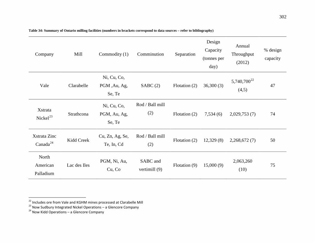
302

Table 34: Summary of Ontario milling facilities (numbers in brackets correspond to data sources – refer to bibliography)

Company Mill Commodity (1) Comminution Separation

Design

Capacity

(tonnes per

day)

Annual

Throughput

(2012)

% design

capacity

Vale Clarabelle

Ni, Cu, Co,

PGM ,Au, Ag,

Se, Te

SABC (2) Flotation (2) 36,300 (3) 5,740,70022

47

(4,5)

Xstrata

Nickel23 Strathcona

Ni, Cu, Co,

PGM, Au, Ag,

Se, Te

Rod / Ball mill

(2)

Flotation (2) 7,534 (6) 2,029,753 (7) 74

Xstrata Zinc

Canada24 Kidd Creek

Cu, Zn, Ag, Se,

Te, In, Cd

Rod / Ball mill

(2) Flotation (2) 12,329 (8) 2,268,672 (7) 50

North

American

Palladium

Lac des Iles PGM, Ni, Au,

Cu, Co

SABC and

vertimill (9) Flotation (9) 15,000 (9)

2,063,260

(10) 75

22 Includes ore from Vale and KGHM mines processed at Clarabelle Mill 23 Now Sudbury Integrated Nickel Operations – a Glencore Company 24 Now Kidd Operations – a Glencore Company

303

St Andrew

Goldfields

Ltd.

Holt Au, Ag SABC (11) CIL-EW (11) 3,000 (11) 897,508 (12) 82

Kirkland

Lake Gold

Inc.

Macassa Au, Ag Ball mill (13) CIP (14) 1,315 (14) 275,840 (15) 59

Brigus Gold

Corp. Black Fox Au Ball mill (16)

CIC, CIL,

CIP (16) 2,200 (17) 735,573 (18) 91

Lake Shore

Gold Corp. Bell Creek Au Ball mill (19)

CIL, CIP

(19) 2,000 (19) 719,298 (20) 98

Goldcorp Inc. Dome Au Rod / Ball mill

(21) CIP (21)

11,000

(21)

4,162,438

(22) 103

Richmont

Mines Inc. Island Gold Au Ball mill (23) CIP (24) 850 (24) 246,743 (25) 81

Wesdome

Gold Mines

Ltd.

Eagle River Au Ball mill (26) Merril-

Crowe (27) 1,000 (27) 219,935 (28) 120

304

Barrick Gold

Corp. Hemlo Au SABC (2) CIP (2)

10,000

(29)

3,080,799

(30) 84

Goldcorp Inc. Musselwhite Au, Ag

Rod / Ball mill

(2)

CIP (2) 4,500 (31) 1,299,600

(22) 79

Goldcorp Inc.

Red Lake

Au, Ag

Ball / vertimill

(32) CIP (32)

3,100 (33) 858,100 (22) 76

Campbell Rod/ball mill (32)

Flotation,

CIP, CIL

(32)

Total 110,129 24,571,519 61

305

Electricity data was then requested from each of these operations, however not all facilities

responded to the request, whereas others were unable to fulfill the request due to insufficient sub-

metering between the mine and the mill.

In the absence of electricity data for each of the milling facilities, the part-load curve from

Clarabelle Mill was used in conjunction with cost estimate models (Western Mine 2006) to

assess the potential savings from other milling facilities in Ontario with similar flowsheets.

These included Strathcona and Kidd Creek mills, both operating a comminution circuit, followed

by flotation. It was assumed that part-load operation of these facilities would be similar to that of

Clarabelle Mill. However, the cost estimate models (Western Mine 2006)were used to estimate

the scale effect due to these facilities having different design capacities.

Electricity consumption in kWh/day for a flotation mill with two products was obtained from the

Mining Cost Service Manual (Western Mine 2006) for mills with design capacities ranging from

100 to 80,000 tonnes per day. These values were then converted to specific energy requirements

in kWh/tonne for each throughput value. Subsequently, a model was developed to estimate how

specific energy consumption (kWh/tonne) varied with design capacity (tonnes/day). Then using a

method adapted from Pascoe (1992) and Remer et al (2008), specific electricity consumption at

design capacity was estimated for Strathcona and Kidd Creek mills, scaled down from the

Clarabelle Mill model, as illustrated in (24).

𝒌𝑾𝒉/𝒕𝒐𝒏𝒏𝒆𝑩 = 𝒌𝑾𝒉/𝒕𝒐𝒏𝒏𝒆𝑨 � 𝑪𝑩𝑪𝑨�𝒙 (24)

where 𝑘𝑊ℎ/𝑡𝑜𝑛𝑛𝑒𝐵and 𝐶𝐵corresponded to the specific energy and design capacity of the

unknown plant, 𝑘𝑊ℎ/𝑡𝑜𝑛𝑛𝑒𝐴 and 𝐶𝐴 corresponded to the respective Clarabelle Mill values and

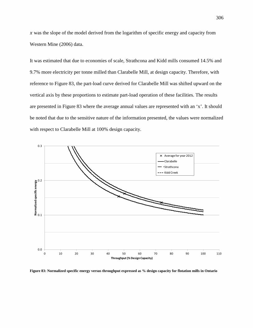
306

𝑥 was the slope of the model derived from the logarithm of specific energy and capacity from

Western Mine (2006) data.

It was estimated that due to economies of scale, Strathcona and Kidd mills consumed 14.5% and

9.7% more electricity per tonne milled than Clarabelle Mill, at design capacity. Therefore, with

reference to Figure 83, the part-load curve derived for Clarabelle Mill was shifted upward on the

vertical axis by these proportions to estimate part-load operation of these facilities. The results

are presented in Figure 83 where the average annual values are represented with an ‘x’. It should

be noted that due to the sensitive nature of the information presented, the values were normalized

with respect to Clarabelle Mill at 100% design capacity.

Figure 83: Normalized specific energy versus throughput expressed as % design capacity for flotation mills in Ontario

0.0

0.1

0.2

0.3

0 10 20 30 40 50 60 70 80 90 100 110

Nor

mal

ized

spec

ific e

nerg

y

Throughput (% Design Capacity)

Average for year 2012

Clarabelle

Strathcona

Kidd Creek

307

Observation of Figure 82 revealed that part-load operation of a mill can lead to a loss of

economies of scale; according to the models, Strathcona Mill which corresponds to the smallest

facility examined had the lowest specific electricity consumption, which is the opposite of what

would be expected. It was also realized that consideration of throughput is important for

benchmarking purposes. For example, comparison of unit electricity consumption before and

after implementation of an energy efficiency measure is only fair when both periods examined

were operated at the same throughput, otherwise it may be difficult to assess the impact of an

initiative on the energy use.

10.7.2 Savings estimate for flotation mills

Using the respective models from Figure 82 and the % design capacity values from Table 34,

potential reductions in energy consumed for census year 2012 were estimated for Strathcona and

Kidd Creek mills. Specific energy consumption savings were estimated by operating each mill at

design capacity to achieve actual reported annual throughput. The results are presented in Table

35. The results for Clarabelle Mill are also presented for comparative purposes. The reductions in

energy consumed translate into reduced energy costs, but not proportionally due to time-of-use

pricing schemes. The savings would be greater if mill operation was maximized during off-peak

rate hours.

308

Table 35: Potential savings from full-load operation for flotation mills in Ontario

Mill % design

capacity

% savings

Clarabelle 47 36

Strathcona 74 16

Kidd Creek 50 32

Additional electricity cost savings arising from load shifting could be obtained by these facilities,

by conserving demand within the 5CP billing rate structure in Ontario. Assuming that a 10%

base load was consumed during periods of no production, it was estimated that the total demand

savings in 2012 from these 3 facilities would total 39 MW, corresponding to over $10 million, in

addition to the electricity savings from Table 35.

It was not possible to derive a part-load operation model for gold milling facilities due to a lack

of information. However, it is estimated that the savings from these facilities would be lower

than those from the flotation mills because most gold mills were operating closer to design

capacity in 2012. However, this estimate is dependent on the slope of the part-load curve.

Although gold mill throughput in terms of % design capacity was higher than base metal mills in

2012, a steeper curve could result in greater savings for the gold processing facilities.

Conversely, a flat curve would yield a lower difference between part-load and full-load specific

energy consumption, thus the savings would also be less. An assessment of the electricity

demand reduction during ‘shut down’ periods could not be undertaken due to the lack of detailed

electricity data from gold milling facilities, thus the demand charge reductions from the 5CP

billing rate could not be estimated.

309

10.8 Discussion of case study findings

An energy audit should not be undertaken simply as a data collection exercise; there needs to be

some checks and balances to provide confidence in the values. This is readily achieved with a

top-down / bottom-up approach. Although the first iteration of the audit may include

assumptions to account for a lack of data, which represent a source of uncertainty, this highlights

data gaps that need additional metering. Then the data can be refined, leading to increased

confidence in the bottom-up audit values. As the uncertainty in the audit values is reduced

confidence grows in understanding energy usage.

During the provincial analysis in this study, several assumptions were made, which may have an

effect on the results. For example, it was assumed that all flotation mills had the same form of

part-load operating curve and that this shifted on the vertical axis only depending on the design

capacity of the facility. Furthermore, mill operation was assumed to be 24 hours per day for 366

days for 2012, unless stated otherwise in the sources reviewed. The reasons for reduced

throughput could include: change in ore mineralogy or properties, lower availability from the

mine, market conditions, or due to maintenance shutdown (scheduled or emergency). It was

assumed in the calculation of % design capacity of the various mills in Table 34 that throughput

was less than design capacity due to low availability. In instances where this may not be the case,

the potential cost and electricity savings estimated in this study may be lower.

Another model (United States Bureau of Mines, Camm 1991) was also examined for estimating

the electricity consumption of operations having different design capacities. Electricity cost

estimates in this model were presented in terms of 1989 $US/short ton but the electricity rate

used to derive the model was not provided. This presented a level of uncertainty when estimating

310

present costs or electricity consumption because either an average index or average electricity

rate was required. Although this was intended to be a cost model, it may be more valuable to

present electricity consumption in energy units (kWh) because these are constant regardless of

time, whereas costs vary with time due to changing tariffs and inflation. In addition, rates vary

depending on location therefore presenting energy units in cost models may be more suitable,

whether it is for electricity or fuel. For this reason, it was decided to use the Western Mine Cost

Service (Western Mine 2006) model in the analysis. Furthermore, the range in throughput values

from the Western Mine cost model was larger than that of the United States Bureau of Mines

(1991).

The efficiency of comminution processes is low; Sadrai et al (2011) reported efficiencies of 1-

2% for grinding and 2-3% for crushing, therefore operation of a mill at less than optimal

conditions, such as lower throughput than design capacity, may result in even lower efficiencies.

The effect of part-load operation of milling facilities was examined during this study and it was

identified that electricity consumption could be improved by ensuring that facilities operated at

design capacity.

The underlying factors that produce the relationship observed in this study between specific

energy consumption and throughput were not investigated. However, it can be hypothesized that

the following measures influence the shape of the part-load curve:

• Most of the equipment used in a milling facility is powered by motors, which operation at

reduced load leads to lower efficiency (Doty, Turner 2009).

• It is estimated that the mass of ore is small compared to the total mass including the ore,

the grinding mill and grinding media. Therefore most of the electricity consumed would

311

be used to rotate the vessel. So an increase in the amount of ore in the mill would not

increase the electricity consumption by the same amount.

• Particle size reduction (grinding) in SAG mills relies on impact and abrasion from steel

balls and ore (Wills, Napier-Munn et al. 2006). Thus unless the amount of steel balls is

increased when there is less ore in the vessel, the chances of particle collision may be

reduced, leading to greater retention time in the mill and thus an increase in the amount

of energy required to achieve a specific target grind.

These three mechanisms (and possibly others) manifest as specific energy consumption versus

throughput expressed in terms of % design capacity.

North American Palladium’s Lac des Iles (LDI) operation has realized that lower throughput

resulted in increased specific energy consumption and thus unit costs, therefore they have

implemented an operating pattern where the ore beneficiation plant operates for 14 days then

shuts down for 14 days and has done so since 2010 (North American Palladium 2013b). This

leads one to ponder whether the plant was designed at the right capacity. Although the flowsheet

for this facility is similar to that of Clarabelle Mill the potential savings were not included in the

analysis of section 7 because of differences in ore mineralogy that may affect electricity

consumption. For example, the target grind for the ore at LDI ranged from 80% passing 38 to

74µm depending on the source (North American Palladium 2013a, McCracken, Kanhai et al.

2013) whereas Clarabelle Mill has a target of 80% passing 150 µm (Lawson, Xu 2011).

Furthermore, in terms of the Bond ball mill work index, the ore at LDI is harder than that treated

at Clarabelle: 17.9 kWh/tonne (McCracken, Kanhai et al. 2013) compared to 12.7 kWh/tonne

(Damjanovic, Goode et al. 2000). For these reasons, it is unknown whether the part-load

operation curve of this facility would be of the same form as that of Clarabelle Mill. But if so, it

312

is estimated that the operating schedule at LDI realized an energy saving of 33%, a figure that

could be compared with those of Table 35.

Others have also investigated inefficiencies arising from part-load operation of individual

processes within a mill. Armstrong (1978) examined the possible energy and cost savings

associated with maximizing the throughput of a rod mill. During a 26 day examination period,

the average specific energy consumption of the rod mill was 3.56 kWh/tonne, whereas the lowest

consumption of 3.00 kWh/tonne was consumed when the mill was operated at rated capacity.

The study demonstrated 16% reduction in specific energy consumption with the mill operating at

maximum throughput, rather than at 61%.

Using the same approach, Armstrong (1980) showed that unit energy consumption increased as

throughput decreased in a uranium mine. The difference between the minimum unit energy

consumption (kWh/tonne) at rated throughput and that at lower production was defined as

“waste energy”. Armstrong showed that elimination of this waste energy by operating at rated

throughput rather than at 72% could lessen the specific energy consumption (kWh/tonne) by

10%. This translated to total electricity cost reduction of 14%, with 8% from peak load control

and 6% from energy savings.

An analysis during an energy audit at Wesfrob Mines Ltd. (now closed) showed that the

relationship between specific electricity consumption (kWh/tonne) and throughput for the total

operation as well as for the separate crushing and grinding stages was inversely related (Doyle

1979); energy savings at the mill could be achieved either by increasing the amount of ore

extracted from the mines or by reducing the plant operating hours.

313

In 1979, a survey of energy consumption in 67 Canadian mills was conducted, including six

nickel and copper ore mills which reported electricity consumption values ranging from 21 to 42

kWh/tonne of ore milled (Joe 1979). These values were compared to those predicted by the

model developed from the Western Mine Cost Service (Western Mine 2006) and it was

determined that only two of the values reported by Joe (1979) agreed with predicted values at

design capacity; the variance between predicted and reported values for these ranged from 1 to

4%. The four values that did not agree with the predictions were appreciably higher than the

model, specifically between 12 and 47%. However, as design capacity was not reported in the

survey, it was not possible to determine whether these facilities were operating at part-load,

which may explain the reason for higher than expected electricity consumption in these cases.

Matthews and Craig (2013) illustrated the benefits of load shifting in a simulated run-of-mine

(ROM) ore milling circuit, operating at 93% capacity. The potential electricity costs savings

estimated in this case ranged from $2.05 to $9.90 per kg of unrefined platinum, for the low and

high tariff periods respectively. These corresponded to savings of 1 to 4 %, however savings for

mills operating at even lower throughputs would be greater. The savings reported by Matthews

and Craig (2013) were consistent with the model developed in this study; at 93% design capacity

it is estimated that electricity consumption was 4% greater than operation at design capacity.

An understanding of electricity billing is important to maximize financial savings from energy

management efforts. For tariffs in Ontario, as illustrated in Table 31 significant cost savings can

result from accurate prediction of peak demand hours, and scheduling of shutdown periods

corresponding to these. Demand response from Class A customers to the 5CP billing structure in

Ontario was examined and presented in the appendix of the Ontario Energy Board Market

Surveillance Panel Monitoring Report (Ontario Energy Board - Market Surveillance Panel 2013).

314

It was estimated, by comparison of pre and post-policy consumption, that a reduction of 200

MW was attributed to the 5CP policy, of which the mining sector contributed 30 MW.

Furthermore, demand reduction from the mining sector during the top 1% demand hours was

estimated at 52 MW, which indicated that these facilities were responding when there was a

chance that a peak demand event would correspond to a coincident peak. Considering that the

average hourly demand from the Ontario mining sector corresponds to about 500 MW (Choi,

Sen et al. 2011) and that the average throughput from milling facilities was 61% of design

capacity in 2012, there appears to still be room for greater response from the mining industry.

However, it is hypothesized that demand reductions during peak demand hours may not be

maximized from the mining sector for the following reasons:

• Changes in operating schedule could lead to issues with labour relations.

• Intermittent schedule may pose operational challenges. For example it may be difficult to

achieve a steady state (temperature, pH…) in certain areas of the process, or shutting

down the mill may have a negative impact on downstream stages.

• Costs of shutting down and restarting operations may exceed financial benefits from the

demand response pricing scheme.

• Contractual obligations may limit the periods for reduced production.

• Organizations may have difficulty in predicting peaks.

• Smaller facilities that do not qualify as Class A are not incentivized to reduce demand to

the same level. Therefore if only a small share of mining companies are classified as

Class A customers, this may hinder demand reductions from the sector but this may

change as a result of lowering the qualification threshold for Class A customers from 5

MW to 3 MW in 2014.

315

Response to coincident peak pricing in Texas was investigated by Zarnikau and Thal (2013) who

illustrated that large electricity consumers had difficulty with predicting and responding to

coincident peaks. The typical response periods corresponded to 2 or 3 hours for a 15 minute peak

interval. In the early years of the coincident pricing rate structure, demand reduction during

peaks varied more than in the later periods. Furthermore, demand increases were observed for

one of the peak periods during the first two years of the program. However, it appeared that

consumers implemented strategies for predicting and responding to coincident peaks, which can

be explained by the increased demand reduction in the latter period of the 5 years examined.

Coincident peak pricing in Ontario was introduced in 2011. This policy is relatively new, thus

customers billed under this structure may still be refining their strategies for maximizing

response during peak hours. Over time, demand response from Class A customers may be

greater.

A review of the Global Adjustment pricing scheme examined alternative methods of recovering

these costs, which included expansion of the current demand response structure to other

consumers in Ontario (Navigant Consulting Ltd. 2014). Although it was suggested by Zarnikau

and Thal (2013) to expand the coincident pricing rate to smaller users, this may make peak

prediction even more difficult. With more users, response may be greater and an anticipated peak

may actually shift to a different period. Changes to the billing structure may also not be effective

at achieving policy goals. As evidenced by Grubler (2012), short-lived policies were not

effective for long- term transitions. This was found by examination of the common

characteristics of successful policies from a total of 20 energy technology innovation case

studies. Similarly, Noailly and Batrakova (2010) stated that policy uncertainty and frequent

changes hindered innovation and investment in building energy efficiency. Consequently, it must

316

be entertained that changes to the current Ontario electricity pricing scheme could reduce the

effectiveness of demand response from firms.

Demand response to coincident peak pricing was also investigated by Liu et al (2013) who

developed an algorithm to assist data centers in minimizing electricity costs. The proposed

strategies to lower peak demand comprised workload shifting and local electricity generation

(behind the ‘meter’). For mining companies operating at full or high capacity, workload shifting

may not be possible. However local electricity generation may present an alternative opportunity

for these organizations to lower electricity costs during coincident peaks.

The analysis in this study was conducted with respect to an energy management perspective with

a basic knowledge of milling practices. Therefore, prior to implementing the strategies from this

study, it would be advisable to consult with plant operators and metallurgists to determine the

optimal conditions to balance energy cost savings against operational limits while maintaining

acceptable metal recovery. The proposed schedule at Clarabelle Mill, operating 11 hours per day,

may not be feasible to implement from an operational or maintenance perspective, but this was

the option that would provide maximum energy savings. Alternatively, a schedule such as that

implemented at LDI, corresponding to a 7 days on, 7 days off, could be investigated. Although

the savings would be lower due to operation during peak hours there still would be savings

compared to operation at part-load, especially if the off days coincide with 5CP hours.

As was demonstrated in Choi et al (2011), from 2005 to 2008 industrial customers in Ontario

implemented load-shifting to reduce consumption during peak rate periods. The amount that

milling facilities specifically have responded to the 5CP billing is unknown thus it is possible

317

that the demand savings estimated in this study have already been realized, but additional

opportunities for energy savings still remain.

10.9 Concluding remarks for case study

Energy penalties are incurred when mills are operated at part-load because more electricity per

tonne of ore milled is consumed, resulting in higher unit operating costs. The first step in

managing energy at a milling facility should correspond to operation at design capacity, ensuring

the most efficient use of electricity. For facilities where throughput may be constrained by the

mining rate, market conditions, operational challenges, etc., this could entail intermittent

operation at 100% design capacity, possibly through alteration of shift patterns. Alternatively, a

modular design including parallel lines could offer throughput flexibility without sacrificing

electricity use per tonne of ore milled.

Although the most efficient use of electricity occurs when a plant is operated at design capacity,

investigation of milling facilities in Ontario revealed that they are not always operated in this

manner. The base metal mills were operated between 47 and 74% of design capacity, whereas

the gold mills ranged from 59 to 120%.

Potential electricity savings from optimizing the schedule to ensure that the base metal flotation

mills in Ontario were always operated at 100% of design capacity could range between 14 and

36%.

An understanding of the billing structure was essential to maximize the financial benefits. These

mills could potentially have also reduced their demand charges by 90% in addition to the

318

electricity savings, by strategically scheduling operation of the mill during non-peak hours, thus

lessening demand during coincident peak hours.

Economies of scale can be lost from low throughput at the larger facilities.

For benchmarking, whether assessing the performance of several facilities, or quantifying

improvements within a single operation as a result of modifications to the equipment or

flowsheet design, only operation at equivalent load values (% design capacity) provides a fair

measure for comparison. In the work reported in this Chapter, a third party undertook an energy

audit which identified ten opportunities for improvement, amounting to 5% of electricity savings.

The work done herein was an audit review which identified further savings of 14% arising from

re-profiling the production schedule. If the current arrangement for demand billing is considered,

additional cost savings of the same scale were identified. The magnitude of these savings will be

important to plant design engineers and plant operators alike.

As part of a continuous improvement process, progressive refinement of energy balances with

the use of a top-down / bottom-up analysis approach lead to increased confidence in the audit

and a stronger basis for future actions. To complete an accurate energy assessment it was

essential to understand the energy data requirements, including the principal controlling factors

governing energy consumption, and how this data can be converted into useful information. In

theory, energy management methodology seems straightforward, but this work has shown that in

practice, a significant amount of effort and analysis was required for a comprehensive and

reliable assessment.

319

11 Using mass and energy balances with pinch analysis principles to identify

energy savings from waste heat recycling: a case study from a

pyrometallurgical mineral processing operation

Although this Chapter is brief, it is included to complete the examination of energy management

in the ‘Mine to Bullion’ process. The work presents a summary of an improved energy audit and

analysis for a pyrometallurgical process and is described in full in Levesque (2011).

In 2008 an energy audit was conducted at Vale’s PTI nickel laterite operation in Indonesia.

However, this audit concluded at the data gathering stage and omitted the analysis stage; thus the

analysis was undertaken as part of a Master’s research project. It was hypothesized that a

substantial amount of energy was wasted from the pyrometallurgical process employed at this

site and that a significant portion of this wasted energy could be captured and used in other

stages of the process (Levesque 2011).

Investigation of this hypothesis began with the conversion of energy data gathered by Vale

personnel into a Sankey diagram to illustrate the energy flows to the various stages in the

process. Subsequently with the use of mass and energy balances, the energy attributed in the

various input and output streams of the process, comprising off-gases and slag, was quantified

and qualified. Complete details of the audit and analysis stages of the study are presented in

Levesque (2011). These energy flows were then added to the Sankey diagram, which illustrated

all energy flows at the site, shown in Figure 83.

320

Figure 84: Sankey diagram from a nickel laterite processing operation (Levesque 2011)25

It can be seen in Figure 83 that most of the energy in the various stages of the process was

released to the atmosphere either via off-gas or slag. With the use of Pinch Analysis principles,

sinks where these sources of waste heat could be used to displace primary energy consumption

were identified. Figure 84 illustrates the proposed scheme for energy reductions via waste heat

recycling.

25 HSFO: High Sulphur Fuel Oil, HSD: High Speed Diesel, BWSTG: Steam turbine, DGB: Diesel generators

321

Figure 85: Sankey diagram from a nickel laterite processing operation with waste heat recycling (Levesque 2011)

Waste heat from the diesel generators as well as from the slag and off-gas from the furnaces was

used to supply the kilns, and the waste heat from the kilns supplied the dryers, thus displacing

HSFO. It can be seen by comparison of Figure 83 and Figure 84 that substantial amounts of

primary energy consumption , specifically HSFO could be reduced with the capture and reuse of

the various waste heat streams within this nickel laterite process. While it should be noted that

technology for waste heat recovery from slag may not yet be commercially available, this

analysis illustrated the potential for savings, thus possibly providing incentive for research in this

area. Table 36 shows the energy conservation potential of the different energy sources from the

proposed waste heat recycling scheme.

322

Table 36: Energy savings from proposed waste heat recycling scheme

Energy source % savings

Coal 0

HSFO 92

HSD 0

Hydro 0

Total26 50

Overall, this analysis shows that substantial savings could be achieved with the reduction of

waste energy by capturing and reusing this energy in other stages of the process. These energy

savings translated to roughly $140 million dollars (2008 US$) in annual cost reductions for this

site (Levesque 2011).

This study also demonstrated the need to follow through on all stages of an energy audit, and it

also showed the importance of assessing the energy associated with mass flows in

pyrometallurgical processes. Gathering primary energy use data without the analysis stage and

identification of other energy sources will not result in the identification of energy conservation

measures. Although this study corresponded to an energy audit for a specific processing route, it

can be applicable to other thermal processes within the mining sector such as smelting.

26 It should be noted that the “Total” corresponds to the % total energy savings at the site. The sum of the % savings from the individual energy sources does not equal the “Total” due to the relative proportion of total energy that these correspond to.

323

12 Discussion

A critical review of energy management progress in the mining sector was conducted by

comparing the conservation measures implemented in the 1970’s with current initiatives. It was

concluded that mining companies were still reporting adoption and implementation of energy

conservation innovations of the 1970’s. Progress in the energy management sector of mining is

thus deemed to be lacklustre.

The main objective for this research was to exemplify parts of a robust energy management

methodology for application within the mining sector as a possible solution to address the slow

evolution. Various energy management components such as communication, auditing and

interpretation were examined, and examples were presented to demonstrate the benefits of the

improved energy management methodology.

12.1 Improved energy audit and analysis guidelines

12.1.1 Recommendations for improved energy audits in the mining sector

Existing energy audit methodologies and guidelines available for energy management were

reviewed and assessed for their applicability to the mining sector. Some of the energy audit

methodologies were of a general nature and could be applied to many different sectors such as

residential, commercial or industrial, whereas other methods were specific to the industrial

sector, but all could be applicable to the mining industry.

Although any of the reviewed audit methods could be used in the mining sector, the choice

would be dependent on the desired level of detail and accuracy, as well as the available

information and resources. For example, conducting a complete bottom-up energy audit in a

324

mine or mining facility may not be easily achieved in the absence of metered values since a

substantial amount of data would be required to estimate the energy consumption from various

end-uses. The use of values derived from estimates for appraisal of potential energy conservation

measures would then introduce uncertainty in the assessment and possibly increase the risk of

implementing the proposed energy conservation initiatives. The energy audit conducted at

Garson Mine from Chapter 7 exemplifies this issue. Energy consumption estimates were used in

areas lacking meters, thus use of the original estimates may have identified “Underground

equipment (drills, bolters…)” electricity use as a priority focus area for potential energy

conservation opportunities. But these savings may not be fully realized when the energy use is

overestimated. The Garson Mine study also highlighted the importance of a data reconciliation

stage in an audit to check estimates which may enhance confidence in the audit values.

Conversely, the use of a top-down method would not produce the same level of detail as the

bottom-up audit unless an iterative process was used, whereby the top-down process was

repeated until energy consumption from all end-uses within each segment was established.

In the Clarabelle Mill case study of Chapter 10, an energy audit was conducted by a consultant

using a bottom-up method, which identified a total of 10 energy conservation measures in

various areas of the plant, with a potential for energy savings totaling 5%. However, most of

these measures corresponded to areas where energy use was not significant, thus having a

minimal impact on total energy use. Alternatively, the top-down energy audit method could have

been used to highlight priority focus areas such as the grinding stage, which may have resulted in

a different outcome with greater savings. Ultimately, the use of a top-down / bottom-up method

to reconcile the data represented a more complete understanding of energy demand at the facility

which was used to augment the potential energy savings by 36%.

325

The reviewed methods in Chapter 4 each presented advantages and disadvantages. Thus the use

of a hybrid method combining the strengths of each type of method may be better suited for the

mining sector. For instance, the use of an iterative methodology combining the top-down and

energy balance methods with the guidelines and tools from the Energy Savings Toolbox and the

Energy Efficiency Opportunities Energy-Mass Balance: Mining documents may be beneficial for

the mining sector. The top-down method would highlight areas where additional focus would be

required, and the energy balance method could be used to allocate energy to various end-uses

within these focus areas in the absence of metered data. The energy balance method would also

ensure that the sum of the amounts from the individual components match the total energy

consumption. The tools and guidelines provided in the Energy Savings Toolbox could be used to

assess energy use and identify potential conservation opportunities, especially if combined with

the mining-specific guidance included in the EEO Energy-Mass Balance: Mining. For example,

the EEO guidance document promoted the use of support variables, which could be incorporated

in the Performance Benchmarks presented in the Energy Savings Toolbox. The Musselwhite

Mine case study presented in Chapter 3.1.6 illustrated how support variables could be used with

energy consumption in an internal benchmarking exercise to assess energy performance within a

mine site. This example demonstrated that the use of energy-influencing variables was necessary

to establish and measure continuous improvement, thus measurement of these variables in

addition to energy use data is necessary.

Another benefit of incorporating the EEO method corresponded to mapping mass flows, which

in the mining sector could present potential energy conservation opportunities. In Chapter 11, an

example using mass and energy balances in a pyrometallurgical mining operation demonstrated

that substantial amounts of energy can be associated with material flows. Quantification of these

326

energy amounts along with qualification of the heat grade allowed use of pinch analysis

principles to link heat sources with heat sinks, thus displacing up to 50% of primary energy

sources at a nickel laterite processing operation.

The iterative part of the proposed hybrid method would comprise repeating the process from the

energy balance step with the next most important focus area; thus this step may satisfy the

continuous improvement aspect of ISO 50001.

12.1.2 A novel energy audit method

A large amount of equipment is used in an underground mine, thus it may not be practical or

economical to install meters on all of these. However, in most mines the total electricity use from

all equipment is metered and a method of extracting information from this data was developed.

Chapter 9 of this work presented a novel disaggregation method that could be used to estimate

the electricity consumption from end-uses in the absence of sub-meter data. This information

could then be used by decision makers and address the lack of information barrier previously

identified.

The novelty of this disaggregation method was the ability to construct the time domain signal

representing the electricity use from a mine hoist as a model. Other existing disaggregation

methods have been used to estimate the total electricity consumption of an end-use or appliance

for a given period by identification of the time when the consumption began and ended, but the

energy use at an exact moment was not determined. Knowledge of an equipment’s load profile

may provide information required for energy management decisions. For example, where a

facility is charged for demand, based on peak demand during a fixed period, an understanding of

327

the disaggregated load profile may be useful for peak shaving or load shifting to lower energy

costs.

The method developed and presented in Chapter 9 was exemplified by estimation of the hoist

electricity consumption, which contributes to the variability of the total energy demand at the

mine. It is presumed that the methodology could be recursively applied to obtain estimates of

other variable loads, such as pumps, compressors, or underground equipment. Thus the method

may be used to discern the variable loads from the baseload or constant energy demands at a

mine.

Although some issues with the developed disaggregation method were identified, it does present

a basis whereby further research could improve the method. Successful development and

adoption of this methodology would reduce the amount of metered data required for energy

audits, thus reducing capital and maintenance costs of sub-metering, as well as costs of data

transmission and storage. An energy audit conducted from data gathered from a single meter

would result in a simpler and lower cost energy management system.

12.2 Improved communication of best practice energy conservation initiatives

The Australian Government’s Energy Efficiency Opportunities (EEO) Act 2006 was a good

initiative to enhance industrial energy efficiency for large consumers. However, in 2014, the bill

was repealed (The Parliament of the Commonwealth of Australia 2014). It was stated that the

program had successfully promoted adoption of energy management as standard practice within

industry, thus mandatory regulation was no longer required. Further incentive for energy

conservation was also driven by rising energy prices. An underpinning element to the

development of the EEO program was to address barriers to identification and adoption of

328

energy efficiency measures, which corresponded to organizational barriers and the lack of

information for decision making. It was stated that for the mining sector “…when energy prices

are low and resource prices are high, energy costs are not considered, because the profits from

greater export volumes far exceed the increased energy costs. When energy prices are high and

the resource price is low the focus changes to minimizing all operating costs, including energy

costs” (The Parliament of the Commonwealth of Australia 2014). Thus it is unknown whether

the abolition of the regulation will sustain the potential for embedded energy management within

the mining sector in Australia.

One of the outcomes of the EEO program was the development of the Mining Significant

Opportunities Register (Australian Government Department of Resources, Energy and Tourism

2011a), which included several examples of energy conservation measures applicable to the

mining sector. A critical review of this register revealed some shortcomings, which were

addressed with the development of the Mining Energy Efficiency Best Practice Database

(Levesque 2013). The improvements comprised i) a standardized reporting mechanism to

facilitate and enhance the identification of relevant information, and ii) a data checking stage

prior to inclusion of case studies in the register to ensure that complete and reliable data was

included.

Dissemination of best practice may be a good mechanism for enhancing energy performance by

addressing the information barrier. However, there are differences between the various mines

and processes within the industry, so the savings reported by one site may not be completely

indicative of those at another facility. Thus the inclusion of additional support variables such as

mine depth, or production amounts would enhance the ability to better estimate the applicability

of measures and the potential savings from one site to another. To date, over 40 users have

329

downloaded a copy of the Mining Energy Efficiency Best Practice Database, and although there

is an option to upload case studies, none have been provided. The reason for this is unknown but

it can be speculated that it may be due to companies already using numerous other reporting

mechanisms such as corporate sustainability reports or corporate websites, or possibly companies

don’t want to disclose all implemented energy conservation measures to maintain

competitiveness.

12.3 Improved interpretation for enhanced energy savings and better

communication

Several sources of data were reviewed, which included the CIPEC Canadian Benchmarking

studies (Canadian Industry Program for Energy Conservation 2005a, Canadian Industry Program

for Energy Conservation 2005b), the US DOE Mining Industry Bandwidth study (U.S.

Department of Energy 2007), resources from Statistics Canada and Natural Resources Canada, as

well as the Canadian Industrial Energy End-use Data and Analysis Center (CIEEDAC) Energy

Use and Related Data reports pertaining to the mining sector (Canadian Industrial Energy End-

use Analysis Center (CIEEDAC) var.). The energy data from these sources pertained to the

mining sector or sub-sectors thereof but the lack of support variable information hindered the

usefulness of the figures. For example, the data presented in Figure 2 seems inconsistent with an

understanding of energy use in the mining sector; the data showed that although diesel

consumption was increasing, electricity use was declining. One would expect that the

consumption from these types of energy would be directly proportional since increased diesel

would require additional ventilation to support safe working conditions. From an energy

management perspective these data may indicate that mining companies have focused efforts at

reducing electricity consumption but that these savings have been eroded or ‘spent’ through

330

increased diesel use and higher ventilation load. However, the lack of support variables in the

available collated data hinders a sufficiently thorough understanding of energy use in the sector,

to support policy development.

Furthermore, use of alternative metrics in the Canadian Underground Benchmarking study suited

to the industry, such as that illustrated in the Musselwhite case study in Chapter 3.1.6 of this

work which include mine depth, production and heating degree days, could have been useful for

setting energy conservation targets for underground mines. It is assumed that the lack of this type

of information or an alternative, universally agreed, metric may be a limiting factor in adoption

of energy management initiatives in the mining sector since there is no target in sight.

Although establishment of a metric for benchmarking energy use for the sector as a whole may

be of limited use, measures on a sub-sectorial basis, by commodity, may enlighten mining

companies with respect to their energy performance and may motivate low performers to

implement changes or adopt energy management protocols. Conversely, internal benchmarks

comparing energy use from a facility for different periods could be useful for monitoring

performance and measuring improvements (Natural Resources Canada 2009) but support

variables that influence energy use should be included.

The development of baselines or benchmarks would also be useful for demonstrating continuous

improvement, as is required in the adoption of the ISO 50001 energy management standard.

Regardless of adoption of this standard, establishment of baselines is an underpinning element

for participation in rate reduction programs such as the Northern Industrial Electricity Rate

Program (NIERP) (Ministry of Northern Development, Mines and Forestry 2010). Thus the use

of benchmarks could be applicable in multiple programs and protocols.

331

The need for appropriate metrics and benchmarking methodologies for comminution processes

was identified as a priority during a workshop hosted by the Coalition for Eco-Efficient

Comminution (CEEC) (Natural Resources Canada 2015). Possible variables that could be

considered for benchmarking comminution processes may include ore hardness, size reduction

ratio, and amount of ore processed. Thus, eliminating the influence from these variables on

energy use may allow companies to compare and assess the energy performance of various

facilities and processing routes. These benchmarks could be used to motivate energy

management activities or to help inform which processing method should be adopted at the

design stage of the mining cycle.

Although tools such as Portfolio Manager are available for benchmarking energy consumption,

water use and greenhouse gas emissions for buildings (United States Environmental Protection

Agency 2015, Natural Resources Canada 2014), there are no comparable options for mines. The

US Environmental Protection Agency developed Energy Star Energy Performance Indicator for

plants to enable benchmarking of industrial facilities, which may assist with establishment of

energy conservation targets (US Environmental Protection Agency n.d.). Models which

considered variables that influence energy use were developed using production and energy use

from census data, against which facilities can compare their energy performance. Scores ranging

from 1 to 100 are assigned to participating facilities, where a low score indicated margin for

improvement and high scoring facilities were considered energy efficient. Indicators were

available for various industrial facilities but mining was not included in the list. Thus, it could be

argued that the time has come for development of such tools for this sector.

The use of internal benchmarking (kWh/tonne vs throughput) at Clarabelle Mill during the

review of the original energy audit, presented in Chapter 10, identified that lower throughput

332

periods consumed a greater amount of electricity per tonne of ore processed. It was shown that

potential electricity savings corresponding to 36% could be achieved via modification of the

operating schedule of the facility while maintaining the same annual throughput. This would

ensure that mill operation occurred at design capacity, and thus at the most energy efficient

operating point.

In the Clarabelle Mill case study presented in Chapter 10, it was also demonstrated that the

financial savings could be enhanced firstly by understanding electricity tariffs and subsequently

by using this knowledge in development of revised operating schedules. Substantial cost savings

were identified by avoiding electricity demand from milling facilities during peak hours in

Ontario.

Sometimes the proposed measures seem simple but their implementation may be challenging. It

is possible that facilities are not equipped for these solutions or that they need time to adapt to

policies such as the 5CP billing scheme in Ontario. For example, since this tariff structure has

been implemented in 2011, the peak hours have occurred during the summer months, but in the

2014-2015 base period, 3 of the 5 peak hours took place during the winter. Therefore it is

possible that some facilities may not be prepared for intermittent operation during these months

without implementation of mitigation strategies. For example, it may be possible that some

pipelines could freeze if pumps were stopped but the use of a heat trace could enable facilities to

respond to the 5CP billing structure.

As ventilation corresponded to the mine system that consumed the most amount of energy in an

underground mine, this was identified as a priority focus area using the top-down energy audit

method. The ventilation case study in Chapter 8 of this work was used to examine potential

333

energy conservation in auxiliary mine ventilation systems via the use of lower friction plastic

ducting.

Implementation of the principles outlined in the Energy Savings Toolbox maximized the energy

savings in the ventilation system by matching the usage to the requirements, and maximizing the

system efficiency. Matching the use to the need was achieved when consideration was given to

the ventilation system as a whole, including the fan and the duct, which delivered energy savings

via flowrate control. It was shown that regardless of the type of duct used in a given system, use

of a custom fixed-speed fan or a variable speed fan resulted in energy savings compared to the

fixed speed counterpart fan, the typical practice. The energy savings from flowrate control

ranged from 1% to 58% depending on the final duct length. Duct substitution was used to

improve system efficiency with the use of lower friction factor ducting to deliver the same

amount or more air to the work area while consuming less energy. It was shown that energy

savings from use of the plastic duct ranged from 7% to 66% compared to the use of Layflat

ducting. Furthermore, combination of both these energy conservation strategies resulted in

additive energy savings, amounting to 56% to 74%, depending on the final duct length.

The case studies presented in Chapter 9 also demonstrated the value of variable speed fans in

auxiliary systems with multiple fans by reducing the discontinuity in operating costs introduced

by the increased airflow when more than one fan was used in a system. Although the plastic duct

always consumed less energy than the other duct types, the cheapest option when considering

capital and operational costs depended on the number of fans in the system and the project

installation. It was also determined that generalized recommendations for selection of duct types

was not possible for underground mines, thus the model developed during this study was made

available for users to determine the optimal solution for custom situations.

334

The work included in Chapter 9 also demonstrated the importance of accurate flowrate

measurements and consideration of leakage during ventilation surveys that are used to determine

duct friction factors. It was shown that flowrate measurements at proper locations are critical to

quantify the actual amount of air flowing through the duct between the pressure measurement

locations. Use of a flowrate value recorded at a single location may result in over or

underestimation of the flow which will lead to an under or overestimation of the duct friction

factor. Furthermore, an assessment method was proposed for validation of the calculated friction

factor with the use of asperity height measurements and a Moody diagram, thus providing

confidence in the values used for decision making.

12.4 Some final thoughts

The work throughout this doctoral study set out to investigate whether existing resources for

energy management were applicable to the mining sector. Review and use of these tools and

guidelines has demonstrated that existing energy management protocols can be used to

understand energy use and identify potential energy conservation initiatives in the mining sector.

However, these established guidelines were not always used and thus the identified energy

savings are not being maximized.

Another topic of investigation for this research was to determine how energy management

progress could be measured. It was determined that this could be achieved with the use of

support variables, which for an underground mine consisted of throughput, mine depth and

heating degree days. But why has no one else presented this before? No organization wants to

think that they are wasting energy or that their performance is poor so it is suspected that the lack

of benchmarking activities may be part of the cause for slow progress in energy management in

335

the mining sector. However without proper benchmarks to highlight the potential for energy

savings and establish targets, there may be no motivation to change behavior with respect to

energy management within this sector.

Energy management in the mining sector may be a cyclical activity corresponding to periods of

low commodity prices and high energy rates, which imply a short-term view. It is suspected that

behavior changes are required in addition to improved guidelines so that short-, medium-, and

long-term perspectives are included in energy management decisions so that continuous

improvement and energy conservation benefits can be sustained.

336

13 Conclusions

13.1 Conclusions

The Garson Mine audit in Chapter 7 resulted in recommendations for an improved energy audit

methodology for mines, developed from a combination of existing methods and guidelines. This

method was derived by considering the challenges in the mining sector with respect to energy

such as little sub-metering and the large amount of equipment used in the industry. Further

refinements to the methodology may arise from conducting energy audits at other mines which

may lead to the identification of additional improvements.

The improved mine audit from Chapter 7 also highlighted the importance of checking estimates

to enhance the accuracy of the audit data. This was illustrated in the data reconciliation step

which showed that some of the original audit values were either over or underestimated, and thus

may have led to focusing future efforts in the wrong areas. It is recommended that future work

may entail development of methods for data reconciliation for specific demand centers within a

mine.

Experience has revealed that extensive sub-metering is lacking in older mines, and thus

precipitated the development of a method for extracting energy consumption of end-uses from a

main mine’s electricity meter. It was shown that it is possible to isolate the electricity

consumption of a mine hoist from the aggregated signal. Furthermore, construction of the time

domain signal of the extracted end-use can be achieved with this novel method, an important

piece of information for energy management. Although the method was illustrated using an

example to estimate the electricity use of a hoist from an underground mine, future work could

entail: i) development of the method for use with other equipment, and ii) an investigation of use

337

of custom filters. Although it is presumed that the method would be limited to the isolation of

electricity use from activities that have a variable load, this information would still be useful to

categorize activities that contribute to the electricity baseload and those that vary..

The Musselwhite Mine example illustrated how mines can demonstrate energy management

improvement with the use of additional support variables. The work showed that although total

annual energy use at this mine increased, energy conservation efforts were effective. However an

in-depth statistical analysis using daily, weekly, or monthly data rather than annual figures may

be used in the future to refine this example or identify additional support variables. Furthermore,

analysis of the support variables that affect energy use of the separate demand centers may also

be beneficial to improve understanding of energy use in mines. Improved understanding leads to

higher energy savings and enhanced profitability.

The ventilation study in Chapter 8 illustrated a methodology for appraisal of potential energy

conservation measures for auxiliary mine ventilation systems. This was achieved with the

development of a novel model to assess the techno-economic viability of various fan and duct

combinations. The ventilation study illustrated the importance of matching the usage to the need

(with a variable speed fan) as well as adoption of energy efficiency measures (lower friction

factor duct) to maximize energy savings. Although this case study focused on an auxiliary mine

ventilation system, the guidelines would be applicable to other systems in a mine. The model

could be further improved with the addition of a fan database whereby the optimal combination

could be identified.

338

Analysis using the auxiliary ventilation model also demonstrated that the use of variable

frequency drives in auxiliary mine ventilation systems is useful for systems with more than one

fan by reducing the discontinuity in energy use introduced when additional fans are added.

Recommendations for development of a standardized ventilation survey method were proposed

for determination of duct friction factors. This method arose from the simulation of a ventilation

system which included leakage at the joints between the segments of the system, which

highlighted the importance of proper characterization of the flowrate in the duct in deriving a

more accurate estimate of the duct friction factor. As there is no data for comparison of leaks

from different types of ducts with different joint geometries from a standard method, there is thus

a need for testing to determine leakage values that can be used for design purposes as well as an

assessment of the quality of installation for existing ventilation systems.

A method for verification of duct friction factor results obtained from ventilation surveys was

suggested. It was recommended that this be achieved with the use of asperity height

measurements and a Moody diagram. As energy use from ventilation systems in underground

mines is substantial so can the energy savings be substantial but there is a need for accurate data

so that the best decisions can be made. Additional ventilation surveys for various auxiliary

ventilation systems (duct and fan), conducted using a standard methodology would be useful to

assess whether the verification method can be extended to other materials.

The Clarabelle Mill study demonstrated that energy savings can be enhanced with improved

interpretation. This was shown by examination of the influence of throughput on energy use per

tonne of ore milled. An improved understanding of energy-influencing factors and use of an

339

internal performance benchmark lead to the identification of a potential for 36% electricity

savings by adoption of a modified schedule to ensure that operation was at design capacity.

Future work could focus on the examination of barriers or challenges at existing milling facilities

to adoption of batch mode operation, such as the effect on downstream processes, or the impact

on mineral recovery. The identification of potential barriers could lead to further research to

identify solutions to mitigate these issues. Additionally, adoption of design principles that

include parallel production lines of lower capacity may eliminate the need for batch-mode

operation for new facilities.

The milling study also showed that part-load operation is a factor that needs to be considered

when benchmarking facilities. A fair comparison (either internal or external) can only be made

when the % design capacity at which a facility was operated is considered. However, this is not

the only factor to consider for benchmarking purposes; ore hardness, feed size, and product size

are some other variables that could influence energy use in milling plants. Thus it is suggested

that a study be conducted to identify and quantify the effect of support variables that could be

used to benchmark mills.

The energy audit at Clarabelle Mill was improved with the demonstration of a methodology to

reconcile bottom-up and top-down data for improved understanding of energy use. However the

accuracy of the metered data is unknown, thus future work could include the development of

guidelines for accurate data gathering and a review of metering technology applicable to the

mining sector.

This work signposted in Chapter 11 showed the importance of measuring mass flows and their

corresponding temperatures to quantify all energy flows within thermal processes found in the

340

minerals industry. Substantial volumes are present and thus substantial savings can be identified.

However the analysis was conducted only for a nickel laterite pyrometallurgical process, and

thus should be repeated to quantify the amounts of waste heat contained in the various output

streams of other smelters and refineries. Further work could also include a review of

commercially available technologies that could be applicable for waste heat recovery in these

facilities. Research and development for new technologies for waste heat recovery from slag,

should definitely be pursued.

Although there have been several milestone improvements in energy management in the mining

sector, it appears that there has not yet been widespread adoption of best practice measures, since

these are still being put into practice. There seems to be a need for better dissemination of good

practice. Presently, energy conservation measures are mainly communicated via sustainability

reports however the task of reviewing all of these is difficult due to the diversity of practice and

incomplete reporting. Adoption of the Mining Energy Efficiency Best Practice database with its

standardized reporting mechanism will enhance transparency of the mining industry in energy

matters and help it maintain its social license to operate. Development of the Best Practice

Database has resulted in an improved communication tool for enhanced dissemination of energy

conservation opportunities within the mining sector. However adoption of the database to date

has been one-sided as no case studies have been uploaded by practitioners or operators for

inclusion. Thus to ensure the success of this tool, enhanced promotion of the register with mine

energy managers or consultants is recommended. Alternatively, a survey could be conducted to

examine the reason for reluctance from mining companies to share best practices whereby

possible solutions could be identified to overcome the barriers to sharing best practices.

341

The review of existing mining energy-related data has revealed that improved reporting with the

inclusion of support variables is required for better communication and better interpretation of

energy use within the sector. Although the data published for the mining sector and sub-sectors

by government and other sources is useful, it does lack in reporting of support variables which

are essential for understanding of trends. For example, the data in Figure 2 may be interpreted

several ways; industry focus was on electricity savings but these translated to increased use of

diesel equipment, or there are more open pit mines in the latter years which contributed to the

rise in diesel use. Thus inclusion of support variables as well as timely reporting of data is

essential to i) examine, and ii) gain a better understanding of recent trends.

The Canadian government has published statistics relating to the mining industry for many years.

Although there is plenty of data, not all the information required for a complete energy efficiency

analysis is available. Although CIEEDAC has published energy consumption by source as well

as production for sub-sectors within the mining industry, other factors of influence are still

needed for a complete energy efficiency assessment.

Innovative solutions will be required for mining companies that are committed to continuous

improvement, motivating investment in research and development in energy management.

However there are few reliable complete data sets available to researchers on energy use in the

mining industry that include factors which influence energy consumption. Consistent

benchmarking and reporting is critical for the industry to progress. Otherwise, the advancement

of new energy management innovations will be hindered, as resources will be misdirected. A

synthesis or audit, not for individual operations or companies, but across the entire mining

industry is required to confirm whether best practices are increasing. It appears that innovation in

terms of energy management in the mining sector has been slow since companies are still

342

reporting energy conservation initiatives that were identified during the 1970’s. Thus maybe

there is a need for an improved curriculum that would highlight energy matters to future mining

engineers, which could then be considered during the design stage of a mining project.

Although the data presented herein indicates a lack of progress in energy management in the

mining sector as a whole, it is known that some companies have implemented highly

sophisticated energy management measures. However these systems still require enhanced

interpretation to direct resources to realize their full potential for energy savings.

Will the mining sector be proactive and voluntarily adopt these changes in corporate policy or

will it be required to do so through increased regulation? Based on the lack of progress identified

from past experiences in the mining sector it is presumed that these changes will likely occur as a

result of regulations or from market conditions such as energy rate increases or lower commodity

prices.

13.2 Contributions

The main objective of this research was to develop an improved energy management

methodology for the mining processing stages from ‘Mine to Bullion’. Several contributions

have emerged through the steps taken to reach this goal and are presented in the following.

13.2.1 Mine

1. The Garson Mine audit resulted in recommendations for an improved energy audit

methodology for mines, developed from a combination of existing methods and

guidelines.

343

2. The improved mine audit also highlighted the importance of checking estimates to

enhance the accuracy of the audit data.

3. A methodology was developed to disaggregate the electricity use within a mine for use in

the absence of sub-metered data.

4. The Musselwhite Mine example illustrated how mines can demonstrate energy

management improvement with the use of additional support variables.

5. The ventilation study illustrated a methodology for appraisal of potential energy

conservation measures for auxiliary mine ventilation systems.

6. Recommendations for development of a standardized method for determination of duct

friction factors.

7. A method for verification of duct friction factor results obtained from ventilation surveys

was suggested.

8. Analysis using the ventilation model demonstrated that the use of variable frequency

drives in auxiliary mine ventilation systems is useful for systems with more than one fan

by reducing the discontinuity in energy use introduced when additional fans are added.

13.2.2 Processing

9. The Clarabelle Mill study demonstrated that energy savings can be enhanced with an

improved interpretation method.

344

10. This study also showed that part-load operation is a factor that needs to be considered

when benchmarking facilities.

11. The energy audit method was improved with the demonstration of a methodology to

reconcile bottom-up and top-down data for improved understanding of energy use.

13.2.3 Purification

12. The work in Chapter 11 showed the importance of measuring mass flows and their

corresponding temperatures to quantify all energy flows within a thermal process, which

could represent substantial amounts and thus substantial savings.

13.2.4 All stages from ‘Mine to Bullion’

13. Development of the Best Practice Database has resulted in an improved communication

tool for enhanced dissemination of energy conservation opportunities within the mining

sector.

14. The review of existing mining energy-related data has revealed that improved reporting

with the inclusion of support variables is required for better communication and better

interpretation of energy use within the sector.

13.3 Future work

The research undertaken during this work has identified that substantial energy savings could be

achieved with the adoption of improved energy management guidelines. Although the work

proposed an improved framework, additional work to further improve the method. Suggestions

from the various chapters and discussion sections are consolidated in the following.

345

13.3.1 Mine

• Further refinements to the energy audit methodology for mines may arise from

conducting audits at other mines which may lead to the identification of additional

improvements.

• It is recommended that future work may entail development of methods for data

reconciliation for specific demand centers within a mine.

• Although the novel energy audit method illustrated an example to estimate the electricity

use of a hoist from an underground mine, future work could entail: i) development of the

method for use with other equipment, and ii) an investigation of use of custom filters.

• Benchmarking for underground mines could benefit from an in-depth statistical analysis

using daily, weekly, or monthly data rather than annual figures. Additional support

variables need to be indentified for underground mines and these could include: mine

depth, production, heating degree days, cooling degree days, and geothermal gradient.

Investigation of the stripping ratio, haulage distances, production, and climate condition

could be used to establish benchmarks for open-pit mines. Furthermore, analysis of the

support variables that affect energy use of the separate demand centers may also be

beneficial to improve understanding of energy use in mines.

• The auxiliary ventilation model developed during this study could be further improved

with the addition of a fan database whereby the optimal combination could be identified.

• As there is no data for comparison of leaks from different types of ducts with different

joint geometries from a standard method, there is thus a need for testing to determine

leakage values that can be used for design purposes as well as an assessment of the

quality of installation for existing ventilation systems.

346

• Since energy use from ventilation systems in underground mines is substantial, so can the

energy savings but there is a need for accurate data so that the best decisions can be

made. Additional ventilation surveys for various duct types, conducted using a standard

methodology would be useful to assess whether the verification method proposed herein

can be extended to other materials.

• Future work for energy audits could also include the development of guidelines for

accurate data gathering and a review of metering technology applicable infrastructure to

the mining sector.

13.3.2 Processing

• Future work could focus on the examination of barriers or challenges at existing milling

facilities to adoption of batch mode operation, such as the effect on downstream

processes, or the impact on mineral recovery. The identification of potential barriers

could lead to further research to identify solutions to mitigate these issues. Additionally,

adoption of design principles that include parallel lines may eliminate the need for batch-

mode operation for new facilities.

• As was demonstrated during this study, benchmarks are a valuable indicator of

performance and can be useful to drive energy management by illustrating the potential

for savings. Thus it is suggested that a study be conducted to identify and quantify the

effect of support variables that could be used to benchmark mills. For milling facilities

the variables could include: ore hardness, production, and size reduction ratio.

347

13.3.3 Purification

• Further work could also include a review of commercially available technologies that

could be applicable for waste heat recovery in pyrometallurgical facilities, as well as

research and development for new technologies for waste heat recovery from slag, not yet

commercially available.

13.3.4 All stages from ‘Mine to Bullion’

• To ensure the success of the Best Practice database enhanced promotion of the register

with mine energy managers or consultants is recommended. Alternatively, a survey could

be conducted to examine the reason for reluctance from mining companies to share best

practices whereby possible solutions could be identified to overcome these barriers.

• Inclusion of support variables as well as timely reporting of data is essential to i)

examine, and ii) gain a better understanding of recent trends. Although CIEEDAC has

published energy consumption by source as well as production for sub-sectors within the

mining industry, other factors of influence are still needed for a complete energy

efficiency assessment.

• Additionally, it may be beneficial to understand why energy management in the mining

sector is of a cyclical nature; occurring when commodity prices are low. Energy savings

exist regardless of metal values thus the industry may not be realizing maximized profits.

348

References

ABB, 2014-last update, ABB commissions Clarabelle mill upgrade for Vale in Canada. Available: http://www.abb.com/cawp/seitp202/c2baacc29b1dfc9b85257c77004ee178.aspx [4/30/2015, 2015].

AKBARI, H., 1995. Validation of an algorithm to disaggregate whole-building hourly electrical load into end uses. Energy, 20(12), pp. 1291-1301.

AKBARI, H. and KONOPACKI, S.J., 1998. Application of an End-Use Disaggregation Algorithm for Obtaining Building Energy-Use Data. Journal of Solar Energy Engineering, 120(3), pp. 205-210.

ALLEN, C., 2012. Applying automation technology to underground ventilation systems. lecture edn. September 2, Sudbury, Dynamic Earth: CIM Distinguished Lecturers Program.

AMBROSIO, S., 2012. Steel spiral ducting friction factor determination. Journal of the Mine Ventilation Society of South Africa, 65(2), pp. 12-19.

AMERICAN SOCIETY OF MECHANICAL ENGINEERS (ASME), 2015-last update, Standards. Available: https://www.asme.org/shop/standards#itemName=Energy%20Efficiency,tax=f07c3937-7eb2-4822-8753-17505c152ee2 [02/14/2015, 2015].

ARMSTRONG, T.B., 1980. Two steps to energy management. CIM Bulletin, (March), pp. 154-159.

ARMSTRONG, T.B., 1978. Energy consumption in mining-milling. Canadian Mining Journal, 99(3),.

AUSTRALIAN GOVERNMENT DEPARTMENT OF RESOURCES, ENERGY AND TOURISM, 2011a-last update, Energy Efficiency Opportunities - Mining. Available: http://www.ret.gov.au/energy/efficiency/eeo/industry-sector/mining/Pages/Mining%20Sector.aspx [03/30/2012] .

AUSTRALIAN GOVERNMENT DEPARTMENT OF RESOURCES, ENERGY AND TOURISM, 2011b-last update, Energy Efficiency Opportunities Program - About the Program. Available: http://www.ret.gov.au/energy/efficiency/eeo/about/Pages/default.aspx [03/30/2012] .

AUSTRALIAN GOVERNMENT DEPARTMENT OF RESOURCES, ENERGY AND TOURISM, 2010-last update, Energy-Mass Balance: Mining. Available: http://www.ret.gov.au/energy/efficiency/eeo/resmaterial/Pages/default.aspx [1/22/2013, 2013].

BALDWIN, C., 2014. Certifiable gains in efficiency. CIM Magazine, 9(6), pp 46.

http://www.abb.com/cawp/seitp202/c2baacc29b1dfc9b85257c77004ee178.aspx�

https://www.asme.org/shop/standards#itemName=Energy%20Efficiency,tax=f07c3937-7eb2-4822-8753-17505c152ee2�

https://www.asme.org/shop/standards#itemName=Energy%20Efficiency,tax=f07c3937-7eb2-4822-8753-17505c152ee2�

http://www.ret.gov.au/energy/efficiency/eeo/industry-sector/mining/Pages/Mining%20Sector.aspx�

http://www.ret.gov.au/energy/efficiency/eeo/industry-sector/mining/Pages/Mining%20Sector.aspx�

http://www.ret.gov.au/energy/efficiency/eeo/about/Pages/default.aspx�

http://www.ret.gov.au/energy/efficiency/eeo/resmaterial/Pages/default.aspx�

349

BARRETTE, R., TAYLOR, A., DOUCET, J., SHELEGEY, J., SULLIVAN, H. and LAWSON, V., 2012. Applying a customer-based approach at Vale's Clarabelle Mill, 44th Annual Canadian Mineral Processors Operators Conference, 17-19 January, 2012 2012, CIM, pp. 39.

BARTSCH, E., LAINE, M. and ANDERSEN, M., 2010. The Application and Implementation of Optimized Mine Ventilation on Demand (OMVOD) at the Xstrata Nickel Rim South Mine, Sudbury, Ontario, HARDCASTLE & MCKINNON, ed. In: 13th United States / North American Mine Ventilation Symposium, June 13-17 2010 2010.

BATTELLE COLUMBUS LABORATORIES, 1975. Energy use patterns in metallurgical and nonmetallic mineral processing (phase 4 - energy data and flowsheets, high-priority commodities). Washington: Bureau of Mines U.S. Department of the Interior.

BENNETT, M. and NEWBOROUGH, M., 2001. Auditing energy use in cities. Energy Policy, 29(2), pp. 125-134.

BERGES, M., GOLDMAN, E., MATTHEWS, H., SOIBELMAN, L. and ANDERSON, K., 2011. User-Centered Nonintrusive Electricity Load Monitoring for Residential Buildings. Journal of Computing in Civil Engineering, 25(6), pp. 471-480.

BIRT, B.J., NEWSHAM, G.R., BEAUSOLEIL-MORRISON, I., ARMSTRONG, M.M., SALDANHA, N. and ROWLANDS, I.H., 2012. Disaggregating categories of electrical energy end-use from whole-house hourly data. Energy and Buildings, 50(0), pp. 93-102.

BOART LONGYEAR, 2014-last update, 2014 Drilling Equipment Product Line. Available: http://app.boartlongyear.com/brochures/Rig_Catalog_English_Feb_28_2014.pdf [6/5/2015, 2015].

BOLL, S.F., 1979. Suppression of acoustic noise in speech using spectral subtraction. IEEE Transactions on Acoustics, Speech, and Signal Processing, ASSP-27(2), pp. 113-120.

BP, 2012-last update, Historical Data. Available: http://www.bp.com/liveassets/bp_internet/globalbp/globalbp_uk_english/reports_and_publications/statistical_energy_review_2011/STAGING/local_assets/spreadsheets/statistical_review_of_world_energy_full_report_2012.xlsx [10/12/2012].

BROWN, A.M., 2001. A step-by-step guide to non-linear regression analysis of experimental data using a Microsoft Excel spreadsheet. Computer methods and programs in biomedicine, 65(3), pp. 191-200.

BROWNLEE, C., 2012. OMA Energy Committee. email edn.

CANADA DEPARTMENT OF TRADE AND COMMERCE, 1945. Chronological Record of Canadian Mining Events from 1604 to 1943 and Historical Tables of the Mineral Production of Canada. Ottawa: Edmond Cloutier.

http://app.boartlongyear.com/brochures/Rig_Catalog_English_Feb_28_2014.pdf�

http://www.bp.com/liveassets/bp_internet/globalbp/globalbp_uk_english/reports_and_publications/statistical_energy_review_2011/STAGING/local_assets/spreadsheets/statistical_review_of_world_energy_full_report_2012.xlsx�



350

CANADA DEPARTMENT OF TRADE AND COMMERCE, 1939. Historical Tables of the Mineral Production of Canada. Ottawa: J.O. Patenaude.

CANADA MINING INNOVATION COUNCIL (CMIC), 2010. Report on the opportunities for demand management in Canadian mining and metalurgical facilities. 18 pages edn.

CANADIAN INDUSTRIAL ENERGY END-USE ANALYSIS CENTER (CIEEDAC), var.-last update, Energy use and related data: Canadian Mining and Metal Smelting and Refining Industires, 1990-various. Available: http://www2.cieedac.sfu.ca/publications [04/25/2013].

CANADIAN INDUSTRIAL ENERGY END-USE ANALYSIS CENTER (CIEEDAC), 2013-last update, CIEEDAC Database on Energy, Production and Intensity Indicators for Canadian Industry. Available: http://www3.cieedac.sfu.ca/CIEEDACweb/mod.php?mod=NAICSPublic&menu=1602 [04/25/2012].

CANADIAN INDUSTRY PROGRAM FOR ENERGY CONSERVATION, 2005a. Benchmarking the Energy Consumption of Canadian Open-Pit Mines. Ottawa: Natural Resources Canada.

CANADIAN INDUSTRY PROGRAM FOR ENERGY CONSERVATION, 2005b. Benchmarking the Energy Consumption of Canadian Underground Bulk Mines. Ottawa: Natural Resources Canada.

CANADIAN INSTITUTE FOR ENERGY TRAINING, 2006. Energy Codes and Standards. Certified Energy Manager Training edn. The Association of Energy Engineers.

CAPEHART, B.L., TURNER, W.C. and KENNEDY, W.J., 2012. Guide to energy management. 7th edn. Lilburn, GA: Fairmont Press.

CHANG, H., YANG, H. and LIN, C., 2008. Load identification in neural networks for a non-intrusive monitoring of industrial electrical loads. In: W. SHEN, J. YONG, Y. YANG, J.P. BARTHES and J. LUO, eds, Computer Supported Cooperative Work in Design IV, 11th International Conference, CSCWD 2007, Melbourne, Australia, April 26-28, 2007. Revised Selected Papers. Springer, pp. 664-674.

CHOI, W., SEN, A. and WHITE, A., 2011. Response of industrial customers to hourly pricing in Ontario's deregulated electricity market. Journal of Regulatory Economics, 40(3), pp. 303-323.

CLEAN ENERGY MINISTERIAL, 2014-last update, Global energy managemetnt system implementation: Case study New Gold New Afto Mine. Available: http://www.cleanenergyministerial.org/Portals/2/pdfs/GSEP_EMWG_New-Gold_case-study.pdf [December 15, 2014].

COOREMANS, C., 2011. Make it strategic! Financial investment logic is not enough. Energy Efficiency, 4(4), pp. 473-492.

http://www2.cieedac.sfu.ca/publications�

http://www3.cieedac.sfu.ca/CIEEDACweb/mod.php?mod=NAICSPublic&menu=1602�

http://www.cleanenergyministerial.org/Portals/2/pdfs/GSEP_EMWG_New-Gold_case-study.pdf�

351

CUBEX LTD., nd.-last update, Orion specification sheet. Available: http://www.cubex.net/cubex/wp-content/uploads/403-10-r13-orion-spec-sheet.pdf [6/4/2015, 2015].

CUBEX LTD., 2010a-last update, Aries Technical Specification. Available: http://www.cubex.net/cubex/wp-content/uploads/Cubex-Aries-Specification-March-22-2010.pdf [6/4/2015, 2015].

CUBEX LTD., 2010b-last update, Cubex Underground Drills R110 Booster Specifications. Available: http://www.cubex.net/cubex/wp-content/uploads/R110-Specifications-Completed-03-22-2010.pdf [6/5/2015, 2015].

CULLAIN, J.G., 1979. Energy conservation at Inco metals company: compressed air in underground mining. CIM Bulletin, 72(811), pp. 70-73.

CURRY, J.A., ISMAY, M.J.L. and JAMESON, G.J., 2014. Mine operating costs and the potential impacts of energy and grinding. Minerals Engineering, 56, pp. 70-80.

DA CUNHA, I.F., 2007-last update, Implementing a sustainable compressed air leak program - Lessons learned and best practices. Available: http://www.oma.on.ca/en/publications/resources/Compressed_Air_Final_070919.pdf [03/12/2012].

DAMJANOVIC, B., GOODE, J.R. and CANADIAN INSTITUTE OF MINING, METALLURGY AND PETROLEUM, 2000. Canadian Milling Practice CIM Special Volume 49. Montreal: Canadian Institute of Mining, Metallurgy and Petroleum.

DE LA HARPE, J.H., CHESSOR, E. and DU PLESSIS, J.J.L., 2014. Chapter 7 Basic Fan Engineering. In: J.J.L. DU PLESSIS, ed, Ventilation and Occupational Environmental Engineering in Mines. 3rd edn. Johannesburg: Mine Ventilation Society of South Africa, pp. 109.

DEBEERS CANADA, ca. 2011-last update, 2010 Report to Society Canada. Available: http://www.debeerscanada.com/files_3/publications.php [03/14/2012].

DEMUTH, H., BEALE, M. and HAGAN, M., 2008. Neural network toolbox™ 6 User’s guide. Natick, MA: The MathWorks, Inc.

DESHPANDE, M.V., 1966. Elements of Electrical Power Station Design. Great Britain: Pitman.

DESOUZA, E., 2004. Auxiliary ventilation operation practices, R. GANGULI and S. BANDOPADHYAY, eds. In: Mine Ventilation: Proceedings of teh 10th US/North American Mine Ventiation Symposium, 16-19 May 2004, A.A. Balkema Publishers, Taylor & Francis Routledge, pp. 341-349.

http://www.cubex.net/cubex/wp-content/uploads/403-10-r13-orion-spec-sheet.pdf�

http://www.cubex.net/cubex/wp-content/uploads/Cubex-Aries-Specification-March-22-2010.pdf�

http://www.cubex.net/cubex/wp-content/uploads/R110-Specifications-Completed-03-22-2010.pdf�

http://www.cubex.net/cubex/wp-content/uploads/R110-Specifications-Completed-03-22-2010.pdf�

http://www.oma.on.ca/en/publications/resources/Compressed_Air_Final_070919.pdf�

http://www.debeerscanada.com/files_3/publications.php�

352

DIAVIK DIAMOND MINE, n.d.-last update, Infrastructure. Available: http://www.diavik.ca/ENG/ouroperations/565_infrastructure.asp [03/12/2012].

DOTY, S. and TURNER, W.C., 2009. Energy Management Handbook. 7th edn. Lilburn, GA: The Fairmont Press.

DOUCET, J., PRICE, C., BARRETTE, R. and LAWSON, V., 2010. Evaluating the effect of operational changes at the vale canada clarabelle mill, 2010, Metallurgical Society of CIM, pp. 373-380.

DOYLE, D.M., 1979. Approach to energy management at Falconbridge nickel mines Limited CIM Bulletin, 72(810), pp. 82-91.

DUCKWORTH, I.J., LOOMIS, I. and PROSSER, B., 2012. Fifteen years of resistance data collected at Freeport Indonesia, F. CALIZAYA and M. NELSON, eds. In: 14th U. S. /North American Mine Ventilation Symposium, 30 June 2012, University of Utah.

DUCKWORTH, I.J. and LOWNDES, I.S., 2003. Modelling of auxilliary ventilation systems. Transactions of the Institutions of Mining and Metallurgy, Section A: Mining Technology, 112(2), pp. A105-A113.

ECKELMAN, M.J., 2010. Facility-level energy and greenhouse gas life-cycle assessment of the global nickel industry. Resources, Conservation & Recycling, 54(4), pp. 256-266.

EGARTER, D., SOBE, A. and ELMENREICH, W., 2013. Evolving non-intrusive load monitoring. In: A.E.A. ESPARCIA-ALCAZAR, ed, Applications of Evolutionary Computation, 16th European Conference, EvoApplications 2013, Vienna, Austria, April 3-5, 2013. Proceedings. Springer, pp. 182-191.

ENERGY MINES AND RESOURCES CANADA, various-last update, Energy Management Series [Homepage of Office of Energy Efficiency], [Online]. Available: http://oee.nrcan.gc.ca/commercial/energy-management-series/6030 [6/3/2012].

FARHAT, A.A. and UGURSAL, V.I., 2010. Greenhouse gas emission intensity factors for marginal electricity generation in Canada. International Journal of Energy Research, 34(15), pp. 1309-1327.

FARINACCIO, L. and ZMEUREANU, R., 1999. Using a pattern recognition approach to disaggregate the total electricity consumption in a house into the major end-uses. Energy and Buildings, 30(3), pp. 245-259.

FEDERAL, PROVINCIAL AND TERRITORIAL SOCIAL LICENCE TASK GROUP, 2010-last update, Mining Sector Performance Report 1998-2008. Available: http://www.nrcan.gc.ca/sites/www.nrcan.gc.ca.minerals-metals/files/pdf/mms-smm/pubr-pubr/pdf/EMMC_english.pdf [03/08/2012].

http://www.diavik.ca/ENG/ouroperations/565_infrastructure.asp�

http://oee.nrcan.gc.ca/commercial/energy-management-series/6030�

http://www.nrcan.gc.ca/sites/www.nrcan.gc.ca.minerals-metals/files/pdf/mms-smm/pubr-pubr/pdf/EMMC_english.pdf�

http://www.nrcan.gc.ca/sites/www.nrcan.gc.ca.minerals-metals/files/pdf/mms-smm/pubr-pubr/pdf/EMMC_english.pdf�

353

FIRTH, S., LOMAS, K., WRIGHT, A. and WALL, R., 2008. Identifying trends in the use of domestic appliances from household electricity consumption measurements. Energy and Buildings, 40(5), pp. 926-936.

FITZPATRICK, P., FONSECA, A. and MCALLISTER, M.L., 2011. From the Whitehorse Mining Initiative Towards Sustainable Mining: lessons learned. Journal of Cleaner Production, 19(4), pp. 376-384.

FLOWER, J.R. and LINNHOFF, B., 1978. Synthesis of heat exchanger networks - 2. Evolutionary generation of networks with various criteria of optimality. AICHE Journal, 24(4), pp. 642-654.

FLSMIDTH, 2013-last update, FLSmidth Smelting equipment. Available: http://www.flsmidth.com/en-US/Industries/Categories/Products/Pyroprocessing/Smelting+equipment/Smelting+equipment [4/30/2015, 2015].

FONSECA, A., MCALLISTER, M.L. and FITZPATRICK, P., 2014. Sustainability reporting among mining corporations: a constructive critique of the GRI approach. Journal of Cleaner Production; Special Volume: The sustainability agenda of the minerals and energy supply and demand network: an integrative analysis of ecological, ethical, economic, and technological dimensions, 84, pp. 70-83.

FRANK, R., BERNANKE, B., OSBERG, L., CROSS, M. and MACLEAN, B., 2012a. Principles of Macroeconomics. 4th Cdn ed. edn. Toronto, Canada: McGraw-Hill Ryerson.

FRANK, R., BERNANKE, B., OSBERG, L., CROSS, M. and MACLEAN, B., 2012b. Principles of Microeconomics. 4th Cdn ed. edn. Toronto, Canada: McGraw-Hill Ryerson.

FYTAS, K., PERREAULT, S. and DAIGLE, B., 2000. EOLAVAL, a mine ventilation planning tool, G.N. PANAGIOTOU and T.N. MICHALAKOPOULO, eds. In: Mine Planning and Equipment Selection 2000 (MPES) - Proceedings of the Ninth International Symposium<br />, 6-9 November 2000 2000, A.A. Balkema Publisher, pp. 51.

G+ INDUSTRIAL PLASTICS INC., nd. G+ Speed Air Duct. Promotional poster edn.

G+ INDUSTRIAL PLASTICS INC., 2014-last update, Ventilation. Available: http://www.plastiquesgplus.com/en/ventilation [March 28, 2014].

GILLIES, A.D. and WU, H.W., 1999. A comparison of air leakage prediction techniques for auxiliary ventilation ducting systems, JERRY CHEN-JEN TIEN, ed. In: Proceedings 8th US mine ventilation symposium, June 11- 17 1999, University of Missouri-Rolla Press, pp. 681.

GLOBAL REPORTING INITIATIVE, ca. 2013-last update, What is GRI?. Available: https://www.globalreporting.org/information/about-gri/what-is-GRI/Pages/default.aspx [02/07/2015, 2015].

http://www.flsmidth.com/en-US/Industries/Categories/Products/Pyroprocessing/Smelting+equipment/Smelting+equipment�

http://www.flsmidth.com/en-US/Industries/Categories/Products/Pyroprocessing/Smelting+equipment/Smelting+equipment�

http://www.plastiquesgplus.com/en/ventilation�

https://www.globalreporting.org/information/about-gri/what-is-GRI/Pages/default.aspx�

354

GLOBAL REPORTING INITIATIVE, ca. 2012-last update, Sustainability Disclosure Database - Search. Available: http://database.globalreporting.org/search [10/31/2012, 2012].

GLOBAL REPORTING INITIATIVE, 2011-last update, Sustainability Reporting Guidelines Version 3.1. Available: https://www.globalreporting.org/resourcelibrary/G3.1-Sustainability-Reporting-Guidelines.pdf [07/04/2012].

GLOBAL REPORTING INITIATIVE, 2010-last update, Mining and Metals Sector Supplement. Available: https://www.globalreporting.org/reporting/sector-guidance/mining-and-metals/Pages/default.aspx [11/1/2012].

GOLDCORP, ca. 2011-last update, Musselwhite - Overview & Operating Highlights. Available: http://www.goldcorp.com/Unrivalled-Assets/Mines-and-Projects/Canada-and-US/Operations/Musselwhite/Overview-and-Operating-Highlights/default.aspx [3/16/2012].

GOLDCORP, ca. 2010-last update, Musselwhite Mine Sustainability Report 2008-2009. Available: http://csr.goldcorp.com/2010/docs/2009_musselwhite.pdf [03/09/2012].

GOLDCORP, ca. 2005-last update, Musselwhite Mining. Available: http://209.89.176.189/operations/musselwhite/mining/ [3/16/2012, 2012].

GOLDCORP, 2011-last update, Rockbreaking News. Available: http://www.porcupinegoldmines.ca/en/latestnewsletter.asp [10/16/2012].

GOLDCORP, 2010-last update, Energy Initiatives at Musselwhite. Available: http://csr.goldcorp.com/2010/6_energy.php#3 [3/22/2012].

GOVERNMENT OF ONTARIO, 2014-last update, Ontario Regulation 126/14 [Homepage of Ontario], [Online]. Available: http://www.e-laws.gov.on.ca/html/source/regs/english/2014/elaws_src_regs_r14126_e.htm [May 8, 2014].

GRUBLER, A., 2012. Energy transitions research: Insights and cautionary tales. Energy Policy, 50(0), pp. 8-16.

GUERIN, T., 2006. A survey of sustainable development initiatives in the Australian mining and minerals industry. Minerals and Energy - Raw Materials Report, 20(3-4), pp. 11-44.

HALL, J.A. and LIEDTKA, S.L., 2007. the Sabanes-Oxley Act: Implications for Large-Scale IT Outsourcing. Communications of the ACM, 50(3), pp. 95-100.

HALL, E.H., HANNA, W.T., REED, L.D., VARGA JR., J., WILLIAMS, D.N., WILKES, K.E., JOHNSON, B.E., MUELLER, W.J., BRADBURY, E.J. and FREDERICK, W.J., 1975. Evaluation of the theoretical potential for energy conservation in seven basic industries. Columbus: Battelle Columbus Laboratories;.

http://database.globalreporting.org/search�

https://www.globalreporting.org/resourcelibrary/G3.1-Sustainability-Reporting-Guidelines.pdf�

https://www.globalreporting.org/resourcelibrary/G3.1-Sustainability-Reporting-Guidelines.pdf�

https://www.globalreporting.org/reporting/sector-guidance/mining-and-metals/Pages/default.aspx�

https://www.globalreporting.org/reporting/sector-guidance/mining-and-metals/Pages/default.aspx�

http://www.goldcorp.com/Unrivalled-Assets/Mines-and-Projects/Canada-and-US/Operations/Musselwhite/Overview-and-Operating-Highlights/default.aspx�

http://www.goldcorp.com/Unrivalled-Assets/Mines-and-Projects/Canada-and-US/Operations/Musselwhite/Overview-and-Operating-Highlights/default.aspx�

http://csr.goldcorp.com/2010/docs/2009_musselwhite.pdf�

http://209.89.176.189/operations/musselwhite/mining/�

http://www.porcupinegoldmines.ca/en/latestnewsletter.asp�

http://csr.goldcorp.com/2010/6_energy.php#3�

http://www.e-laws.gov.on.ca/html/source/regs/english/2014/elaws_src_regs_r14126_e.htm�

http://www.e-laws.gov.on.ca/html/source/regs/english/2014/elaws_src_regs_r14126_e.htm�

355

HARR, M.E., 1987. Reliablitiy-based design in civil engineering. United States of America: McGraw Hill.

HARRIS, J.H. and ARMSTRONG, T.B., 1979. Electrical energy management Inco metals company Shebandowan Mine. CIM Bulletin, 72(812), pp. 66-72.

HARTMAN, H.L. and MUTMANSKY, J.M., 2002. Introductory mining engineering. Second edition edn. New Jersey, U.S.A.: John Wiley & Sons.

HASANBEIGI, A. and PRICE, L., 2010-last update, Industrial Energy Audit Guidebook: Guidelies for Conducting an Energy Audit in Industrial Facilities [Homepage of Ernest Orlando Lawrence Berkeley National Laboratory], [Online]. Available: http://minotaur.lbl.gov/china.lbl.gov/sites/china.lbl.gov/files/LBNL-3991E.Industrial%20Energy%20Audit%20Guidebook_0.pdf [04/01, 2013].

HAUTA, R., 2015. MacLean drilling time. email edn.

HAYS, R.M., 1990. Trucks. In: B.A. KENNEDY, ed, Surface Mining. 2nd edition edn. Littleton, CO, USA: Society of Mining, Metallurgy, and Exploration, pp. 672-691.

ICMM, 2015-last update, Member performance. Available: http://www.icmm.com/members/member-performance [5/25/2015, 2015].

ICMM, 2013-last update, The cost of carbon pricing: competitiveness implications for the mining and metals industry. Available: http://www.icmm.com/publications [26 September, 2013].

ICMM, 2012a-last update, 10 principles. Available: http://www.icmm.com/our-work/sustainable-development-framework/10-principles [10/31/2012].

ICMM, 2012b-last update, About ICMM. Available: http://www.icmm.com/ [07/03/2012].

ICMM, 2012c-last update, Member companies. Available: http://www.icmm.com/members [10/31/2012].

ICMM, 2012d-last update, Our History. Available: http://www.icmm.com/about-us/icmm-history [10/31/2012].

ICMM, 2012e-last update, Public reporting. Available: http://www.icmm.com/our-work/sustainable-development-framework/public-reporting [11/2/2012].

IESO, 2014a-last update, Global Adjustment. Available: http://www.ieso.ca/imoweb/b100/b100_GA.asp [February 19, 2014].

http://minotaur.lbl.gov/china.lbl.gov/sites/china.lbl.gov/files/LBNL-3991E.Industrial%20Energy%20Audit%20Guidebook_0.pdf�

http://minotaur.lbl.gov/china.lbl.gov/sites/china.lbl.gov/files/LBNL-3991E.Industrial%20Energy%20Audit%20Guidebook_0.pdf�

http://www.icmm.com/members/member-performance�

http://www.icmm.com/publications�

http://www.icmm.com/our-work/sustainable-development-framework/10-principles�

http://www.icmm.com/our-work/sustainable-development-framework/10-principles�

http://www.icmm.com/�

http://www.icmm.com/members�

http://www.icmm.com/about-us/icmm-history�

http://www.icmm.com/about-us/icmm-history�

http://www.icmm.com/our-work/sustainable-development-framework/public-reporting�

http://www.icmm.com/our-work/sustainable-development-framework/public-reporting�

http://www.ieso.ca/imoweb/b100/b100_GA.asp�

356

IESO, 2014b-last update, Global Adjustment for Class A. Available: http://www.ieso.ca/Pages/Participate/Settlements/Global-Adjustment-for-Class-A.aspx [February 19, 2014].

IESO, 2013a-last update, Demand Response. Available: http://www.ieso.ca/imoweb/siteShared/managing_demand.asp?sid=bi [8/1/2013, 2013].

IESO, 2013b-last update, Electricity Charges Explained. Available: http://www.ieso.ca/imoweb/role/wholesaleCharges.asp [8/1/2013, 2013].

IESO, 2013c-last update, Energy Market Overview. Available: http://www.ieso.ca/imoweb/mktOverview/mktOverview.asp [8/1/2013, 2013].

IESO, 2013d-last update, Why Wholesale Prices Fluctuate. Available: http://www.ieso.ca/imoweb/businessIndustry/bi_wholesale_price2.asp [8/1/2013, 2013].

INSTITUTE FOR INDUSTRIAL PRODUCTIVITY, 2012-last update, Tools. Available: http://www.iipnetwork.org/tools [6/15/2012].

INTERNATIONAL ORGANIZATION FOR STANDARDIZATION, 2011a-last update, Discover ISO. Available: http://www.iso.org/iso/about/discover-iso_isos-name.htm [09/07/2011].

INTERNATIONAL ORGANIZATION FOR STANDARDIZATION, 2011b-last update, Energy management systems - Requirements with guidance for use. Available: http://www.iso.org/iso/iso_catalogue/catalogue_tc/catalogue_detail.htm?csnumber=51297 [July 22, 2011].

JAMES, B., 1978. Energy efficiency - high of low priority for management in the industrial minerals industry? CIM Bulletin, 71(800), pp. 97-103.

JENKINS, H. and YAKOVLEVA, N., 2006. Corporate social responsibility in the mining industry: Exploring trends in social and environmental disclosure. Journal of Cleaner Production, 14(3–4), pp. 271-284.

JOE, E.G., 1979. Energy consumption in Canadian mills. CIM Bulletin, 72(806), pp. 147-151.

KERR, A., BOUCHARD, A.P., TRUSKOSKI, J., BARRETT, J. and LABONTE, G., 2003. The "Mill Redesign Project" at Inco's Clarabelle mill. CIM Bulletin, 96(1075), pp. 58-66.

KIM, H., MARWAH, M., ARLITT, M., LYON, G. and HAN, J., 2011. Unsupervised Disaggregation of Low Frequency Power Measurements. Society for Industrial and Applied Mathematics, pp. 747-758.

LAMBERT, E.H., 1973. Energy conservation for the mining industry. CIM Bulletin, 66(738), pp. 69-74.

http://www.ieso.ca/Pages/Participate/Settlements/Global-Adjustment-for-Class-A.aspx�

http://www.ieso.ca/imoweb/siteShared/managing_demand.asp?sid=bi�

http://www.ieso.ca/imoweb/role/wholesaleCharges.asp�

http://www.ieso.ca/imoweb/mktOverview/mktOverview.asp�

http://www.ieso.ca/imoweb/businessIndustry/bi_wholesale_price2.asp�

http://www.iipnetwork.org/tools�

http://www.iso.org/iso/about/discover-iso_isos-name.htm�

http://www.iso.org/iso/iso_catalogue/catalogue_tc/catalogue_detail.htm?csnumber=51297�

357

LANDRY, B.J., 2009. Energy Survey Report Calarabelle Mill Vale Inco Ltd. Draft Report edn. Byron J. Landry & Associates.

LAWSON, V. and XU, M., 2011. Float it, clean it, depress it - Consolidating the separation stages at Clarabelle Mill, Metallurgical Plant Design and Operating Strategies, METPLANT 2011, August 8, 2011 - August 9, 2011 2011, Australasian Institute of Mining and Metallurgy, pp. 589-601.

LCG MANAGEMENT GROUP, 2009-last update, Investigation of Current Research Related to the Reduction of Energy Usage in Mines Trhough Recycling, Reuse, and Other Means. Available: http://www.miningexcellence.ca/doc/b0410238-4883-44e7-858f-a97f3d924501 [09/26/2011].

LE ROUX, W., 1979. Mine ventilation notes for beginners. Third ediction edn. South Africa: Mine Ventilation Society of South Africa.

LEVESQUE, M., 2013-last update, Mining Energy Efficiency Best Practice Database. Available: http://www.mirarco.org/scripts/Mining_EE_Best_Practice/index.php [08/09/2013, 2013].

LEVESQUE, M.Y. and MILLAR, D.L., 2015a-last update, Auxiliary mine ventilation cost assessment model [Homepage of Laurentian University], [Online]. Available: http://dx.doi.org/10.14285/10219/2301 [02/10, 2015].

LEVESQUE, M. and MILLAR, D.L., 2013. A best practice database for energy management in the minerals industry, World Mining Congress, 11-15 August 2013, Canadian Institute of Mining, Metallurgy and Petroleum.

LEVESQUE, M., 2011. Understanding Mine Heat - Sankey Diagrams for Nickel Production from Laterite Ore, Laurentian University.

LEVESQUE, M.Y. and MILLAR, D.L., 2015b. The link between operational practices and specific energy consumption in metal ore milling plants – Ontario experiences. Minerals Engineering, 71(0), pp. 146-158.

LEVESQUE, M., MILLAR, D. and PARASZCZAK, J., 2014. Energy and mining – the home truths. Journal of Cleaner Production, 84(0), pp. 233-255.

LI, G., KOCSIS, C. and HARDCASTLE, S., 2011. Sensitivity analysis on parameter changes in underground mine ventilation systems. Journal of Coal Science and Engineering, 17(3), pp. 251-255.

LIANG, J., NG, S.K.K., KENDALL, G. and CHENG, J.W.M., 2010a. Load signature studypart I: Basic concept, structure, and methodology. IEEE Transactions on Power Delivery, 25(2), pp. 551-560.

http://www.miningexcellence.ca/doc/b0410238-4883-44e7-858f-a97f3d924501�

http://www.mirarco.org/scripts/Mining_EE_Best_Practice/index.php�

http://dx.doi.org/10.14285/10219/2301�

358

LIANG, J., NG, S.K.K., KENDALL, G. and CHENG, J.W.M., 2010b. Load signature studypart II: Disaggregation framework, simulation, and applications. IEEE Transactions on Power Delivery, 25(2), pp. 561-569.

LINNHOFF, B., 1993. Pinch analysis - a state-of-the-art overview. Chemical Engineering Research and Design, 71, pp. 503-522.

LINNHOFF, B. and HINDMARSH, E., 1983. Pinch design method for heat exchanger networks. Chemical Engineering Science, 38(5), pp. 745-763.

LINNHOFF, B. and FLOWER, J.R., 1978. Synthesis of heat exchanger networks - 1. systematic generation of energy optimal networks. AICHE Journal, 24(4), pp. 633-642.

LIU, Z., WIERMAN, A., CHEN, Y., RAZON, B. and CHEN, N., 2013. Data center demand response: Avoiding the coincident peak via workload shifting and local generation. Performance Evaluation, 70(10), pp. 770-791.

LYNN, P.A., 1989. An introduction to the analysis and processing of signals. 3rd edition edn. Houndmills, Basingstoke, Hampshire, London: Macmillan Education Ltd.

MALLETT, R., 2014. Garson Mine Energy Audit. Masters (M.Eng.) project in Natural Resources Engineeringq edn. Sudbury, Canada: Laurentian University.

MANIAN, V.S., 1974. Energy efficiency brings economies. Canadian Mining Journal, 95(9), pp. 37, 58-37, 58.

MARCEAU, M.L. and ZMEUREANU, R., 2000. Nonintrusive load disaggregation computer program to estimate the energy consumption of major end uses in residential buildings. Energy Conversion and Management, 41(13), pp. 1389-1403.

MASON, J.K., WHITE, G.D., O'BRIEN, M.S. and KOMAR, C., 2003. Report of Activities 2002. Resident Geologist Program, Thunder Bay North Regional Resident Geologist Report edn. Thunder Bay North District; Ontario Geological Survey, Open File Report 6111.

MASON, J.K., WHITE, G.D., SCOTT, J.F., O'BRIEN, M.S. and KOMAR, C., 2002. Report of Activities 2001. Resident Geologist Program, Thunder Bay North Regional Resident Geologist Report edn. Thunder Bay North District; Ontario Geological Survey, Open File Report 6080.

MATTHEWS, B. and CRAIG, I.K., 2013. Demand side management of a run-of-mine ore milling circuit. Control Engineering Practice, 21(6), pp. 759-768.

MCCRACKEN, T., KANHAI, T., BRIDSON, P., MCBRIDE, W.R., SMALL, K. and PENNA, D.N., January 31, 2013-last update, Technical Report Lac des Iles Mine, Ontario, Incorporating Prefeasibility Study Offset Zone Phase I [Homepage of Tetra Tech], [Online]. Available: http://www.nap.com/investors/investor-briefcase/default.aspx [November 28, 2013].

http://www.nap.com/investors/investor-briefcase/default.aspx�

359

MCLELLAN, B.C., CORDER, G.D., GIURCO, D.P. and ISHIHARA, K.N., 2012. Renewable energy in the minerals industry: a review of global potential. Journal of Cleaner Production, 32(0), pp. 32-44.

MCPHERSON, M.J., 1993. Subsurface ventilation and environmental engineering. 1 edn. London: Chapman and Hall.

MECANICAD, nd.-last update, Ventilation. Available: http://mecanicad.ca/en/content/ventilation [6/7/2015, 2015].

METKEMEYER, L., 2012. Inproving copper recovery in heap leaching cycles in hydrometallurgical plants by solar heating, WIERTZ, J. & FILIPPO, G., ed. In: Enermin2012: 2nd International Seminar on Energy Management in the Mining Industry, 10-12 September 2012 2012, Gecamin.

MEYER, C.F., 1990. Determining the friction losses of underground ventilation ducting. Journal of the Mine Ventilation Society of South Africa, 43(10), pp. 191-195.

MILLAR, D.L., LEVESQUE, M., LYLE, G. and BULLOCK, K., 2012. Enabling progressive energy managemnet practice for minerals operations. CIM Journal, 3(3), pp. 178-184.

MINE VENTILATION SERVICES, 2003. DuctSIM User's Manual. Version 1.0b edn.

MINERALS AND METALS SECTOR OF NATURAL RESOURCES CANADA AND THE NATIONAL ENERGY BOARD, 2012. Principal Mineral Areas of Canada, Sixty-first Edition, 2011. Geological Survey of Canada, Map 900A, scale 1: 6 000 000.

MINING ASSOCIATION OF CANADA, 2013-last update, F&F 2012 Facts & Figures of the Canadian Mining Industry. Available: http://www.mining.ca/site/index.php/en/ [1/31/2013].

MINING ASSOCIATION OF CANADA, 2012a-last update, Energy and GHG Emissions Management Guidance Document. Available: http://www.mining.ca/site/index.php/en/towards-sustainable-mining/performance-measures-a-protocols.html [11/1/2012].

MINING ASSOCIATION OF CANADA, 2012b-last update, Energy and GHG Emissions Management Protocol. Available: http://www.mining.ca/site/index.php/en/towards-sustainable-mining/performance-measures-a-protocols.html [11/1/2012].

MINING ASSOCIATION OF CANADA, 2011a-last update, Members. Available: http://www.mining.ca/site/index.php/en/about-us/members.html [11/1/2012].

MINING ASSOCIATION OF CANADA, 2011b-last update, Performance Measures and Protocols. Available: http://www.mining.ca/site/index.php/en/towards-sustainable-mining/performance-measures-a-protocols.html [07/03/2012].

http://mecanicad.ca/en/content/ventilation�

http://www.mining.ca/site/index.php/en/�

http://www.mining.ca/site/index.php/en/towards-sustainable-mining/performance-measures-a-protocols.html�




http://www.mining.ca/site/index.php/en/about-us/members.html�



360

MINING ASSOCIATION OF CANADA, 2011c-last update, Towards Sustainable Mining. Available: http://www.mining.ca/site/index.php/en/towards-sustainable-mining.html [07/03/2012].

MINING ASSOCIATION OF CANADA, 2011d-last update, TSM Progress Report. Available: http://www.mining.ca/site/index.php/en/towards-sustainable-mining/progress-reports.html [11/1/2012].

MINISTRY OF NORTHERN DEVELOPMENT, MINES AND FORESTRY, 2010-last update, Northern Industrial Electricity Rate Porgram (NIER Program) Program Rules. Available: http://www.mndmf.gov.on.ca/northern_development/business_support/northern_industrial_electricity_rate_program_e.asp [09/15/2011].

MUDD, G.M., 2010. Global trends and environmental issues in nickel mining: Sulfides versus laterites. Ore Geology Reviews, 38(1-2), pp. 9-26.

MUDD, G.M., 2007. Global trends in gold mining: Towards quantifying environmental and resource sustainability. Resources Policy, 32(1-2), pp. 42-56.

NAPIER-MUNN, T., 2015. Is progress in energy-efficient comminution doomed? Minerals Engineering; Special issue: Comminution, 73, pp. 1-6.

NATURAL RESOURCES CANADA, nd-last update, Comprehensive Energy Use Database Industrial Sector Disaggregated Industries Canada (2012) [Homepage of Office of Energy Efficiency], [Online]. Available: http://oee.nrcan.gc.ca/corporate/statistics/neud/dpa/menus/trends/comprehensive/trends_id_ca.cfm [5/22/2015, 2015].

NATURAL RESOURCES CANADA, ca. 2014-last update, Energy Use Data Handbook Tables. Available: http://oee.nrcan.gc.ca/corporate/statistics/neud/dpa/menus/trends/handbook/handbook_aaa_ca.cfm [4/29/2015, 2015].

NATURAL RESOURCES CANADA, ca. 2013a-last update, Energy Use Data Handbook Tables [Homepage of Natural Resources Canada], [Online]. Available: http://oee.nrcan.gc.ca/corporate/statistics/neud/dpa/handbook_totalsectors_ca.cfm?attr=0 [06/02/2013, 2013].

NATURAL RESOURCES CANADA, ca. 2013b. RETScreen Plus.

NATURAL RESOURCES CANADA, 2015-last update, Heads Up CIPEC – Volume 19, Issue 1. Available: http://www.nrcan.gc.ca/energy/efficiency/industry/technical-info/library/newsletter/14406#s7 [2/19/2015, 2015].

http://www.mining.ca/site/index.php/en/towards-sustainable-mining.html�

http://www.mining.ca/site/index.php/en/towards-sustainable-mining/progress-reports.html�

http://www.mndmf.gov.on.ca/northern_development/business_support/northern_industrial_electricity_rate_program_e.asp�

http://www.mndmf.gov.on.ca/northern_development/business_support/northern_industrial_electricity_rate_program_e.asp�

http://oee.nrcan.gc.ca/corporate/statistics/neud/dpa/menus/trends/comprehensive/trends_id_ca.cfm�

http://oee.nrcan.gc.ca/corporate/statistics/neud/dpa/menus/trends/comprehensive/trends_id_ca.cfm�

http://oee.nrcan.gc.ca/corporate/statistics/neud/dpa/menus/trends/handbook/handbook_aaa_ca.cfm�

http://oee.nrcan.gc.ca/corporate/statistics/neud/dpa/menus/trends/handbook/handbook_aaa_ca.cfm�

http://oee.nrcan.gc.ca/corporate/statistics/neud/dpa/handbook_totalsectors_ca.cfm?attr=0�

http://www.nrcan.gc.ca/energy/efficiency/industry/technical-info/library/newsletter/14406#s7�

http://www.nrcan.gc.ca/energy/efficiency/industry/technical-info/library/newsletter/14406#s7�

361

NATURAL RESOURCES CANADA, 2014-last update, Why ENERGY STAR Portfolio Manager?. Available: http://www.nrcan.gc.ca/energy/efficiency/buildings/energy-benchmarking/whypm/3729 [2/12/2015, 2015].

NATURAL RESOURCES CANADA, 2012a. General Review of the Mineral Industries. Catalogue no. 26-201-X. 2010 Edition edn.

NATURAL RESOURCES CANADA, 2012b. Heads Up CIPEC Newsletter. newsletter edn. June 1, 2012 ed. Vol. XVI, No. 11.

NATURAL RESOURCES CANADA, 2011a-last update, Canadian Industry Program for Energy Conservation (CIPEC). Available: http://oee.nrcan.gc.ca/industrial/cipec/13673 [3/7/2012].

NATURAL RESOURCES CANADA, 2011b-last update, Canadian Minerals Yearbook (CMY) | Minerals and Metals Sector. Available: http://www.nrcan.gc.ca/minerals-metals/business-market/canadian-minerals-yearbook/4070 [9/16/2013].

NATURAL RESOURCES CANADA, 2009-last update, Energy Savings Toolbox - An Energy Audit Manual and Tool. Available: http://www.nrcan.gc.ca/energy/efficiency/industry/cipec/5161 [04/23/2013, 2013].

NATURAL RESOURCES CANADA, 2003-last update, Pinch Analysis: For the efficient use of energy, water & hydrogen. Available: http://canmetenergy.nrcan.gc.ca/industrial-processes/industrial-systems-optimization/publications/206 [06/07/2012].

NAVIGANT CONSULTING LTD., January 23, 2014-last update, Global Adjustment Review. Available: http://www.ieso.ca/imoweb/pubs/consult/se106/se106-20140128-Global_Adjustment_Review_Report.pdf [January 31, 2014].

NICKELL, C., G. and DENYER, C., 2007. An Introduction to SAS 70 Audits. Benefits Law Journal, 20(1), pp. 58-68.

NOAILLY, J. and BATRAKOVA, S., 2010. Stimulating energy-efficient innovations in the Dutch building sector: Empirical evidence from patent counts and policy lessons. Energy Policy, 38(12), pp. 7803-7817.

NORGATE, T. and HAQUE, N., 2010. Energy and greenhouse gas impacts of mining and mineral processing operations. Journal of Cleaner Production, 18(3), pp. 266-274.

NORTH AMERICAN PALLADIUM, 2013a-last update, 2009 Annual Report. Available: http://www.nap.com/investors/Financial-Reports/default.aspx [11/14, 2013].

NORTH AMERICAN PALLADIUM, 2013b-last update, 2012 Annual Report. Available: http://www.nap.com/investors/Financial-Reports/default.aspx [11/14, 2013].

http://www.nrcan.gc.ca/energy/efficiency/buildings/energy-benchmarking/whypm/3729�

http://www.nrcan.gc.ca/energy/efficiency/buildings/energy-benchmarking/whypm/3729�

http://oee.nrcan.gc.ca/industrial/cipec/13673�

http://www.nrcan.gc.ca/minerals-metals/business-market/canadian-minerals-yearbook/4070�

http://www.nrcan.gc.ca/minerals-metals/business-market/canadian-minerals-yearbook/4070�

http://www.nrcan.gc.ca/energy/efficiency/industry/cipec/5161�

http://canmetenergy.nrcan.gc.ca/industrial-processes/industrial-systems-optimization/publications/206�

http://canmetenergy.nrcan.gc.ca/industrial-processes/industrial-systems-optimization/publications/206�

http://www.ieso.ca/imoweb/pubs/consult/se106/se106-20140128-Global_Adjustment_Review_Report.pdf�

http://www.ieso.ca/imoweb/pubs/consult/se106/se106-20140128-Global_Adjustment_Review_Report.pdf�

http://www.nap.com/investors/Financial-Reports/default.aspx�

http://www.nap.com/investors/Financial-Reports/default.aspx�

362

ONDER, M., SARAC, S. and CEVIK, E., 2006. The influence of ventilation variables on the volume rate of airflow delivered to the face of long drivages. Tunnelling and Underground Space Technology, 21(5), pp. 568-574.

ONTARIO ENERGY BOARD - MARKET SURVEILLANCE PANEL, June, 2013-last update, Monitoring Report on the IESO-Administered Electricity Markets for the period from May 2012 - October 2012, Appendix. Available: http://www.ontarioenergyboard.ca/OEB/Industry/About the OEB/Electricity Market Surveillance/Market Surveillance Panel Reports [7/18/2013, 2013].

ONTARIO PROSPECTORS ASSOCIATION, 2012-last update, Ontario Mining and Exploration Directory 2012. Available: http://www.mndm.gov.on.ca/en/news/mines-and-minerals/ontario-mining-exploration-directory-2012 [November 14, 2013].

PARASZCZAK, J., FYTAS, K. and LAFLAMME, M., 2014. Feasibility of Using Electric Trucks in Deep Metal Mines. Mine Planning and Equipment Selection. Springer, pp. 1265-1275.

PARASZCZAK, J. and FYTAS, K., 2012. Renewable energy sources - a promising opportunity for remote mine sites? International Conference on Renewable Energies and Power Quality (ICREPQ'12), March 28-30 2012 2012.

PASCOE, R.D., 1992. Capital and operating costs of minerals engineering plants - a review of simple estimation techniques. Minerals Engineering, 5(8), pp. 883-893.

PAWLIK, K.E., CAPEHART, L.C. and CAPEHART, B.L., 2002. “Energy Balancing”: How to Use the Energy Balance Data You Have Collected TO MAKE FINANCIAL DECISIONS. Strategic Planning for Energy and the Environment, 21(3), pp. 58-80.

PAWLIK, K.E., CAPEHART, L.C. and CAPEHART, B.L., 2001. Analyzing Facility Energy Use: A Balancing Act. Strategic Planning for Energy and the Environment, 21(2), pp. 8-33.

PERDAN, S. and AZAPAGIC, A., 2011. Carbon trading: Current schemes and future developments. Energy Policy, 39(10), pp. 6040-6054.

PEREZ, F. and SANCHEZ, L.E., 2009. Assessing the Evolution of Sustainablity Reporting in the Mining Sector. Environmental Management, 43(6), pp. 949.

PERRY, R.H., GREEN, D.W. and MALONEY, J.O., 1997. Perry's chemical engineers' handbook. 7th edn. New York: McGraw-Hill.

PICKETT, D.E., HALL, W.S. and SMITH, G.W., 1978. Milling practice in Canada. Montréal, Qué.: Canadian Institute of Mining and Metallurgy.

PIRAINO, G., RIMAWI, E. and CERNY, A., 2012. 25+MWth solar heating commercially viable for solvent extraction electrowinning (SX-EW) and heap leaching, WIERTZ, J. & FILIPPO, G., ed. In: Enermin2012: 2nd International Seminar on Energy Management in the Mining Industry, 10-12 September 2012 2012, Gecamin.

http://www.ontarioenergyboard.ca/OEB/Industry/About�

http://www.mndm.gov.on.ca/en/news/mines-and-minerals/ontario-mining-exploration-directory-2012�

http://www.mndm.gov.on.ca/en/news/mines-and-minerals/ontario-mining-exploration-directory-2012�

363

RAMIREZ, R.W., 1985. The FFT, fundamentals and concepts. Englewood Cliffs, NJ: Prentice-Hall.

REMER, D.S., LIN, S., YU, N. and HSIN, K., 2008. An update on cost and scale-up factors, international inflation indexes and location factors. International Journal of Production Economics, 114(1), pp. 333-346.

RIO TINTO, ca. 2010-last update, Diavik Diamond Mine 2010 Sustainable Development Report. Available: http://www.diavik.ca/ENG/resources/661.asp [03/13/2012].

RIO TINTO, 2013-last update, Wind farm. Available: http://www.diavik.ca/ENG/ouroperations/565_wind_farm.asp [03/07, 2013].

ROSENQVIST, J., THOLLANDER, P., ROHDIN, P. and SODERSTROM, M., 2012. Industrial Energy Auditing for Increased Sustainability: Methodology and Measurements. In: A. GEBREMEDHIN, ed, Sustainable Energy - Recent Studies. InTech, pp. Chapter 5.

SADRAI, S., MEECH, J.A., TROMANS, D. and SASSANI, F., 2011. Energy efficient comminution under high velocity impact fragmentation. Minerals Engineering, 24(10), pp. 1053-1061.

SANDVIK MINING AND CONSTRUCTION, 2007-last update, DL410-10 Technical Specification. Available: http://www.mc.sandvik.com/SANDVIK/1281/Internet/MANorway/SE03605.NSF/Alldocs/Products*5CDrill*rigs*and*rock*drills*5CUnderground*drill*rigs*5CProduction*drill*rigs*2ADL410*2D10/$FILE/7-6100-F (DL410-10).pdf [6/5/2015, 2015].

SAYADI, A.R., KHALESI, M.R. and KHOSFARMAN, M., 2014. A parametric cost model for mineral grinding mills. Minerals Engineering, 55(0), pp. 96-102.

SCALES, M., 2007. Musselwhite mine & mill. Canadian Mining Journal, (June ed.), 128(5), pp. 21-22.

SCOTT, G.D., 2008. Energy Conservation Opportunities in Ontario's Mining Industry. report edn. July 7 2008: Ontario Mining Association's Energy Committee.

SIROIS, L., 1993. Energy Efficiency R&D Opportunities in the Mining and Metallurgy Sector, Phase 1 - Scoping Study. CANMET Contract No. EA9710-2-1. 2012. Ottawa, Ontario: Efficiency and Alternative Energy Technology Branch, CANMET, Natural Resources Canada, NRCan.

SMITH, H., 2008. Modelling for resource and environmental impact assessments of wave farms, University of Exeter.

SMITH, S.W., 1997. The scientist & engineer's guide to digital signal processing. 1 edn. San Diego, Calif: California Technical Pub.

http://www.diavik.ca/ENG/resources/661.asp�

http://www.diavik.ca/ENG/ouroperations/565_wind_farm.asp�

http://www.mc.sandvik.com/SANDVIK/1281/Internet/MANorway/SE03605.NSF/Alldocs/Products*5CDrill*rigs*and*rock*drills*5CUnderground*drill*rigs*5CProduction*drill*rigs*2ADL410*2D10/$FILE/7-6100-F�



364

SMYK, M.C., WHITE, G.D., HINZ, P. and KOMAR, C., 2009. Report of Activities 2008. Resident Geologist Program, Thunder Bay North Regional Resident Geologist Report: Thunder Bay North District edn. Ontario Geological Survey Open File Report 6233.

SMYK, M.C., WHITE, G.D., MAGEE, M.A. and KOMAR, C., 2006. Report of Activities 2005. Resident Geologist Program, Thunder Bay North Regional Resident Geologist Report: Thunder Bay North District edn. Ontario Geological Survey Open File Report 6181.



SMYK, M.C., WHITE, G.D., PUUMALA, M.A., HINZ, P. and KOMAR, C., 2008. Report of Activities 2007. Resident Geologist Program, Thunder Bay North Regional Resident Geologist Report: Thunder Bay North District edn. Ontario Geological Survey Open File Report 6217.

SMYK, M.C., WHITE, G.D., PUUMALA, M.A., MAGEE, M.A. and KOMAR, C., 2007. Report of Activities 2006. Resident Geologist Program, Thunder Bay North Regional Resident Geologist Report: Thunder Bay North District edn. Ontario Geological Survey Open File Report 6201.

SMYK, M.C. and WHITE, L., H.C., 2010. Report of Activities 2009. Resident Geologist Program, Thunder Bay North Regional Resident Geologist Report: Thunder Bay North District edn. Ontario Geological Survey Open File Report 6245.

SONNEMANN, G.W., SCHUHMACHER, M. and CASTELLS, F., 2003. Uncertainty assessment by a Monte Carlo simulation in a life cycle inventory of electricity produced by a waste incinerator. Journal of Cleaner Production, 11(3), pp. 279-292.

STANLEY, W.D., 2005. Technical analysis and applications with MATLAB. Clifton Park, NY: Thomson Delmar Learning.

STATISTICS CANADA, var.a-last update, General Review of the Mineral Industries, Mines, Quarries and Sand Pits. Catalogue no. 26-201-X [Homepage of Ottawa], [Online]. Available: http://www5.statcan.gc.ca/bsolc/olc-cel/olc-cel?catno=26-201-X&chropg=1&lang=eng [9/12/2013].

STATISTICS CANADA, var.b-last update, Non-metal Mines, Catalogue no. 26-224-XIB. Available: http://www5.statcan.gc.ca/bsolc/olc-cel/olc-cel?catno=26-224-XIB&lang=eng [9/12/2013].

http://www5.statcan.gc.ca/bsolc/olc-cel/olc-cel?catno=26-201-X&chropg=1&lang=eng�

http://www5.statcan.gc.ca/bsolc/olc-cel/olc-cel?catno=26-224-XIB&lang=eng�

365

STATISTICS CANADA, var.c-last update, Report on Energy Supply Demand in Canada. Catalogue no. 57-003-X [Homepage of Ottawa], [Online]. Available: http://www5.statcan.gc.ca/bsolc/olc-cel/olc-cel?catno=57-003-X&chropg=1&lang=eng [9/12/2013].

STATISTICS CANADA, var-last update, Metal Ore Mining, Catalogue no. 26-223-X. Available: http://www5.statcan.gc.ca/bsolc/olc-cel/olc-cel?lang=eng&catno=26-223-X [9/12/2013].

STATISTICS CANADA, 2015/01/22, 2015-last update, CANSIM - 326-0021 - Consumer Price Index. Available: http://www5.statcan.gc.ca/cansim/a26?lang=eng&retrLang=eng&id=3260021&paSer=&pattern=&stByVal=1&p1=1&p2=37&tabMode=dataTable&csid= [4/29/2015, 2015].

STATISTICS CANADA, 2013-last update, CANSIM - Canadian socioeconomic database from Statistics Canada. Available: http://www5.statcan.gc.ca/cansim/a01?lang=eng [4/25/2013, 2013].

STATISTICS CANADA, 2012. North American Industry Classification System (NAICS) Canada Catalogue no. 12-501-X. Ottawa, Canada: Minister of Industry.

STATISTICS CANADA, 1999-last update, Historical Statistics of Canada : Chronological index. Available: http://www5.statcan.gc.ca/bsolc/olc-cel/olc-cel?catno=11-516-X&chropg=1&lang=eng#issue1983001 [9/13/2013].

STERLING, D., 2010. Identifying Opportunities to reduce the consumption of energy across Mining and Processing Plants, World Energy Congress 2010, September 12-16 2010 2010.

STREETER, V.L. and WYLIE, E.B., 1983. Fluid mechanics. International Student Edition edn. Tokyo, Japan: McGraw-Hill.

TAMROCK, 2000. TamrockProduct Catalogue- Robolt series technical data sheet.

TAMROCK, 1995. TamrockProduct Catalogue- Drills - Solo series.

TARDIF, D., PAQUET, A. and MILLER, F., 2010. Exploration drift ventilation project at Mine Casa Berardi - A new and more economical solution, HARDCASTLE & MCKINNON, ed. In: 13th U.S./North American Mine Ventilation Symposium, June 13-16 2010 2010, MIRARCO, pp. 243.

TECK, ca. 2007-last update, Sustainability Summary Hemlo Operations. Available: http://www.teck.com/Generic.aspx?PAGE=Teck+Site%2fResponsibility+Pages%2fSustainability+Pages%2fReport+Archive&portalName=tc [03/22/2012].

TENBERGEN, R.A. and THROSSELL, M.A., 1989. Semi autogenous-ball mill-crushing circuit selection for Inco's mills rationalization, A.L. MULAR and G.E. AGAR, eds. In: Advances in

http://www5.statcan.gc.ca/bsolc/olc-cel/olc-cel?catno=57-003-X&chropg=1&lang=eng�

http://www5.statcan.gc.ca/bsolc/olc-cel/olc-cel?lang=eng&catno=26-223-X�

http://www5.statcan.gc.ca/cansim/a26?lang=eng&retrLang=eng&id=3260021&paSer=&pattern=&stByVal=1&p1=1&p2=37&tabMode=dataTable&csid=�

http://www5.statcan.gc.ca/cansim/a26?lang=eng&retrLang=eng&id=3260021&paSer=&pattern=&stByVal=1&p1=1&p2=37&tabMode=dataTable&csid=�

http://www5.statcan.gc.ca/cansim/a01?lang=eng�

http://www5.statcan.gc.ca/bsolc/olc-cel/olc-cel?catno=11-516-X&chropg=1&lang=eng#issue1983001�

http://www5.statcan.gc.ca/bsolc/olc-cel/olc-cel?catno=11-516-X&chropg=1&lang=eng#issue1983001�

http://www.teck.com/Generic.aspx?PAGE=Teck+Site%2fResponsibility+Pages%2fSustainability+Pages%2fReport+Archive&portalName=tc�

http://www.teck.com/Generic.aspx?PAGE=Teck+Site%2fResponsibility+Pages%2fSustainability+Pages%2fReport+Archive&portalName=tc�

366

autogenous and semiautogenous grinding technology, 25-27 September 1989, Dept. of Mining and Mineral Process Engineering, University of British Columbia, pp. 253.

THE ASSOCIATION OF ENERGY ENGINEERS, nd. Comprehensive five day training program for Certified Energy Managers course manual. Atlanta, Georgia, USA: The Association of Energy Engineers.

THE GLOBE AND MAIL, 2010-last update, Teck, Suncor partner on wind power project. Available: http://www.theglobeandmail.com/report-on-business/industry-news/energy-and-resources/teck-suncor-partner-on-wind-power-project/article1718742/ [05/31/2012].

THE MATHWORKS INC., 2014. MATLAB Release 2014a. R2014a edn. Natick, Massachusetts, United States: The MathWorks Inc.

THE MINING ASSOCIATION OF CANADA, ca. 2015-last update, Facts and Figures 2014. Available: http://mining.ca/sites/default/files/documents/Facts_and_Figures_2014.pdf [6/11/2015, 2015].

THE PARLIAMENT OF THE COMMONWEALTH OF AUSTRALIA, 2014-last update, Energy Efficiency Opportunities (Repeal) Bill 2014 Explanatory Memorandum. Available: http://www.aph.gov.au/Parliamentary_Business/Bills_Legislation/Bills_Search_Results/Result?bId=r5232 [3/10/2015, 2015].

THUMANN, A. and MEHTA, D.P., 2008. Handbook of energy engineering. 6th edn. Lilburn, GA: Fairmont Press ;Boca Raton, FL.

TITTMAN, D.W., 1977. ENERGY CONSERVATION AT ERIE MINING CO. Mining Congress Journal, 63(12), pp. 37-41.

TOLLINSKY, N., 2011-last update, Idling alternative cuts diesel consumption [Homepage of Sudbury Mining Solutions Journal, December Issue], [Online]. Available: http://www.sudburyminingsolutions.com/idling-alternative-cuts-diesel-consumption.html [06/28/2012].

TORAÑO ÁLVAREZ, J., RODRÍGUEZ DÍEZ, R., CUESTA GUTIÉRREZ, A. and DIEGO ÁLVAREZ, I., 2002. A computer program for calculating ventilation in tunnelling works based on an explicit method. Tunnelling and Underground Space Technology, 17(3), pp. 227-236.

TRAPANI, K. and MILLAR, D.L., 2013. Proposing offshore photovoltaic (PV) technology to the energy mix of the Maltese islands. Energy Conversion and Management, 67, pp. 18-26.

TUAZON, D., CORDER, G., POWELL, M. and ZIEMSKI, M., 2012. A practical and rigorous approach for the integration of sustainability principles into the decision-making processes at minerals processing operations. Minerals Engineering, 29, pp. 65-71.

http://www.theglobeandmail.com/report-on-business/industry-news/energy-and-resources/teck-suncor-partner-on-wind-power-project/article1718742/�

http://www.theglobeandmail.com/report-on-business/industry-news/energy-and-resources/teck-suncor-partner-on-wind-power-project/article1718742/�

http://mining.ca/sites/default/files/documents/Facts_and_Figures_2014.pdf�

http://www.aph.gov.au/Parliamentary_Business/Bills_Legislation/Bills_Search_Results/Result?bId=r5232�

http://www.aph.gov.au/Parliamentary_Business/Bills_Legislation/Bills_Search_Results/Result?bId=r5232�

http://www.sudburyminingsolutions.com/idling-alternative-cuts-diesel-consumption.html�

367

U.S. DEPARTMENT OF ENERGY, 2007-last update, Mining Industry Energy Bandwidth Study. Available: http://www1.eere.energy.gov/manufacturing/industries_technologies/mining/pdfs/mining_bandwidth.pdf [05/28/2012].

U.S. ENERGY INFORMATION ADMINISTRATION, 2011-last update, Frequently Asked Questions - How much electricity is lost in transmission and distribution in the United States?. Available: http://205.254.135.7/tools/faqs/faq.cfm?id=105&t=3 [07/03/2012].

U.S. GOVERNMENT PRINTING OFFICE, 2002-last update, Public Law 107 - 204 - Sarbanes-Oxley Act of 2002. Available: http://www.gpo.gov/fdsys/pkg/PLAW-107publ204/content-detail.html [4/16/2012].

UGURSAL, I., 2014. Underground mining equipment. Photograph taken during site visit edn. Sudbury, Canada.

UNITED NATIONS GLOBAL COMPACT, 2011-last update, UN Global Compact Brochure - Corporate Sustainability in The Wold Economy. Available: http://www.unglobalcompact.org/AboutTheGC/index.html [07/3/2012].

UNITED NATIONS GLOBAL COMPACT, 2010-last update, GRI and UN Global Compact Forge New Alliance. Available: http://www.unglobalcompact.org/news/50-06-24-2010 [11/31/2012].

UNITED STATES BUREAU OF MINES and CAMM, T.W., 1991. Simplified cost models for prefeasibility mineral evaluations. Washington, DC: U.S. Dept. of the Interior, Bureau of Mines.

UNITED STATES ENVIRONMENTAL PROTECTION AGENCY, 2015-last update, Use Portfolio Manager. Available: http://www.energystar.gov/buildings/facility-owners-and-managers/existing-buildings/use-portfolio-manager [2/12/2015, 2015].

UNIVERSITY OF TORONTO, ONTARIO, LAURENTIAN UNIVERSITY and CANADIAN COMMITTEE ON ELECTROTECHNOLOGIES, 1989. Energy efficient technologies in the mining and metals industry. Toronto, Ont.: Ministry of Energy.

US ENVIRONMENTAL PROTECTION AGENCY, n.d.-last update, ENERGY STAR Energy Performance Indicators for plants. Available: http://www.energystar.gov/buildings/facility-owners-and-managers/industrial-plants/measure-track-and-benchmark/energy-star-energy?s=mega [3/10/2015, 2015].

VALE, ca. 2010-last update, 2010 Sustainability Report. Available: http://nickel.vale.com/sustainability/reports/default.aspx [04/12/2012].

VENTILATION ENGINEER, 2015. k Factor Comparison Generic. email edn.

http://www1.eere.energy.gov/manufacturing/industries_technologies/mining/pdfs/mining_bandwidth.pdf�

http://www1.eere.energy.gov/manufacturing/industries_technologies/mining/pdfs/mining_bandwidth.pdf�

http://205.254.135.7/tools/faqs/faq.cfm?id=105&t=3�

http://www.gpo.gov/fdsys/pkg/PLAW-107publ204/content-detail.html�

http://www.gpo.gov/fdsys/pkg/PLAW-107publ204/content-detail.html�

http://www.unglobalcompact.org/AboutTheGC/index.html�

http://www.unglobalcompact.org/news/50-06-24-2010�

http://www.energystar.gov/buildings/facility-owners-and-managers/existing-buildings/use-portfolio-manager�

http://www.energystar.gov/buildings/facility-owners-and-managers/existing-buildings/use-portfolio-manager�

http://www.energystar.gov/buildings/facility-owners-and-managers/industrial-plants/measure-track-and-benchmark/energy-star-energy?s=mega�



http://nickel.vale.com/sustainability/reports/default.aspx�

368

VETTERLING, W.T., TEUKOLSKY, S.A. and PRESS, W.H., 1992. Numerical recipes in C. Second Edition edn. Cambridge: Press Syndicate of the University of Cambridge.

VOGT, Y., 2003. Top–down Energy Modeling. Strategic Planning for Energy and the Environment, 22(4), pp. 64-79.

VUTUKURI, V., 1984. Design of auxiliary ventilation systems for long drivages, Fifth Australian Tunneling Conference, 22-24 October 1984, Institution of Engineers, Australia, pp. 73.

VUTUKURI, V., 1983. Air leakage in ventilation ducting and the design of auxiliary ventilation systems. Mining Engineer, 143, pp. 37-43.

VUTUKURI, V.S., 1993. Appraisal of accuracy of various formulas for the design of a simple auxiliary ventilation system, Proceedings of the 6th US Mine Ventilation Symposium, June 21, 1993 - June 23, 1993 1993, Publ by SME, pp. 145-150.

WALKER, J. and HOWARD, S., 2002. Finding the way forward. Nottingham, UK: Russell Press Ltd.

WALKER, S.C., 1988. Mine winding and transport. Advances in Mining Science and Technology. Amsterdam: Elsevier Pub. Co, pp.307.

WANG, H.Q., CHEN, S.Q. and CHEN, T., 2010. Study of energy saving of long distance tunnelling fan with frequency control in coal mines. Transactions of the Institutions of Mining and Metallurgy, Section A: Mining Technology, 119(1), pp. 42-45.

WANG, S., YAN, C. and XIAO, F., 2012. Quantitative energy performance assessment methods for existing buildings. Energy and Buildings, 55(0), pp. 873-888.

WENZL, K.H.B., 1978. Inco metals company, Ontario division, energy management program. Canadian Mining Journal, 99(3), pp.11.

WESTERN MINE, 2006. Mining Cost Service. Vol. 1 edn. Washington, USA: Schumacher, Otto.

WIDMANN, A., SCHROGER, E. and MAESS, B., 2014. Digital filter design for electrophysiological data - a practical approach. Journal of neuroscience methods, (In Press),.

WILLS, B.A., NAPIER-MUNN, T., WILLS, B.A. and JULIUS KRUTTSCHNITT MINERAL RESEARCH CENTRE, 2006. Wills' mineral processing technology :an introduction to the practical aspects of ore treatment and mineral recovery. 7th edn. Amsterdam: Elsevier/Butterworth-Heinemann.

369

WINGENDER, J.R. and WOODROOF, E.A., 1997. When firms publicize energy management projects their stock prices go up. Strategic Planning for Energy and the Environment, 17(1), pp. 38-51.

WORKPLACE SAFETY NORTH, 2011. Auxiliary Mine Ventilation Manual. v 1.3 edn. Ontario.

WU, H.W. and GILLIES, A.D., 2014. A comparison of predicted performance of auxiliary ventilation ducting systems, F. VON GLEHN and M. BIFFI, eds. In: Proceedings of the tenth international mine ventilation congress, 2-8 August 2014, The Mine Ventilation Society of South Africa, pp. 533.

XIAO, Z. and VIEN, A., 2003. Limitations of variance analysis using propagation of variance. Minerals Engineering, 16(5), pp. 455-462.

XSTRATA, ca. 2007-last update, Sustainability Report 2007. Available: http://www.xstrata.com/content/assets/pdf/x_sustainability_2007.pdf [03/26/2012].

XSTRATA NICKEL, ca. 2010-last update, Xstrata Nickel Sustainability Report 2010 Sudbury Operations. Available: http://www.xstratanickel.com/EN/Publications/Sustainable%20Development/Xstrata%20Nickel%20Sustainability%20Report%202010_Sudbury.pdf [10/09/2012].

XU, M. and WILSON, S., 2000. Investigation of seasonal metallurgical shift at Inco's clarabelle mill. Minerals Engineering, 13(12), pp. 1207-1218.

YAN, C., WANG, S. and XIAO, F., 2012. A simplified energy performance assessment method for existing buildings based on energy bill disaggregation. Energy and Buildings, 55(0), pp. 563-574.

ZARNIKAU, J. and THAL, D., 2013. The response of large industrial energy consumers to four coincident peak (4CP) transmission charges in the Texas (ERCOT) market. Utilities Policy, 26(0), pp. 1-6.

ZOHA, A., GLUHAK, A., IMRAN, M.A. and RAJASEGARAR, S., 2012. Non-Intrusive Load Monitoring Approaches for Disaggregated Energy Sensing: A Survey. Sensors, 12(12), pp. 16838-16866.

http://www.xstrata.com/content/assets/pdf/x_sustainability_2007.pdf�

http://www.xstratanickel.com/EN/Publications/Sustainable%20Development/Xstrata%20Nickel%20Sustainability%20Report%202010_Sudbury.pdf�

http://www.xstratanickel.com/EN/Publications/Sustainable%20Development/Xstrata%20Nickel%20Sustainability%20Report%202010_Sudbury.pdf�

370

Appendix A – Frames extracted from different months of the aggregated

signal to train Neural Network for identification of hoist operating

probability

371

January

0 5 10 15 20 25 30 350.5

0.6

0.7

0.8

0.9

Time (minutes)

Nor

mal

ized

ele

ctric

ity

0 0.1 0.2 0.3 0.4 0.5 0.6 0.7 0.8 0.9 10

0.05

0.1


Nor

mal

ized

mag

nitu

de

0 5 10 15 20 25 30 350.5

0.6

0.7

0.8

0.9

Time (minutes)

Nor

mal

ized

ele

ctric

ity

0 0.1 0.2 0.3 0.4 0.5 0.6 0.7 0.8 0.9 10

0.05

0.1


Nor

mal

ized

mag

nitu

de

0 5 10 15 20 25 30 350.5

0.6

0.7

0.8

0.9

Time (minutes)

Nor

mal

ized

ele

ctric

ity

0 0.1 0.2 0.3 0.4 0.5 0.6 0.7 0.8 0.9 10

0.05

0.1


Nor

mal

ized

mag

nitu

de

0 5 10 15 20 25 30 350.5

0.6

0.7

0.8

0.9

Time (minutes)

Nor

mal

ized

ele

ctric

ity

0 0.1 0.2 0.3 0.4 0.5 0.6 0.7 0.8 0.9 10

0.05

0.1


Nor

mal

ized

mag

nitu

de

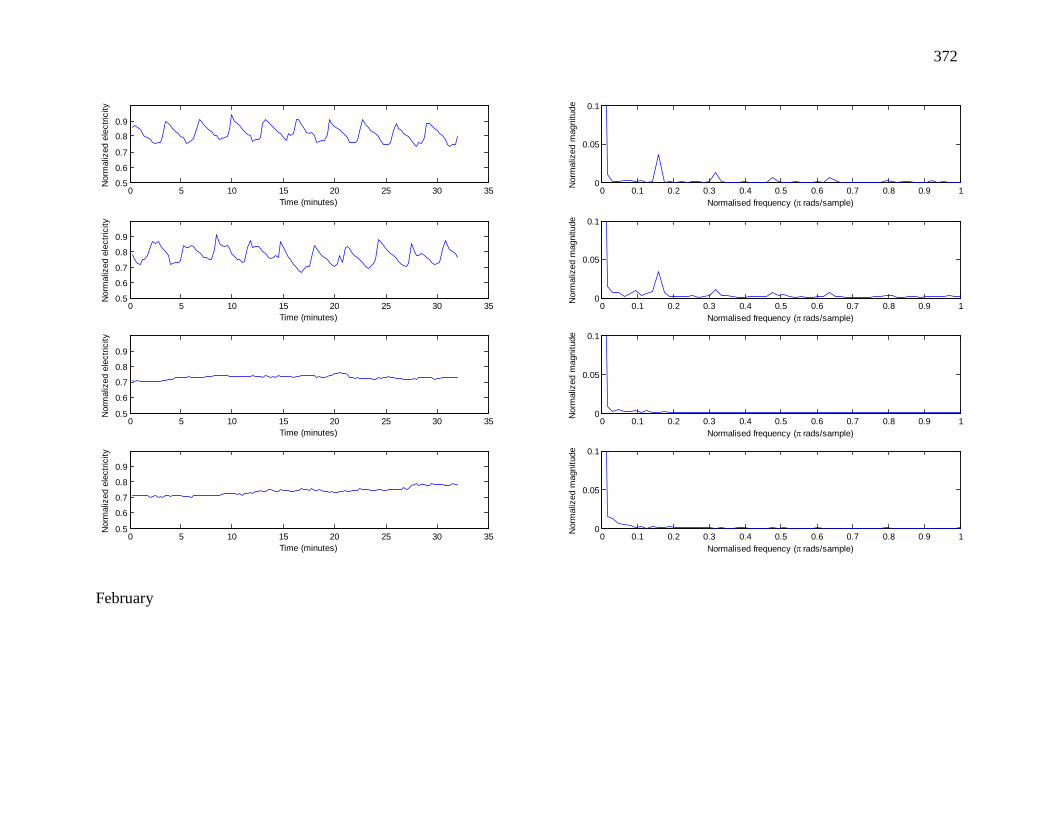
372

February

0 5 10 15 20 25 30 350.5

0.6

0.7

0.8

0.9

Time (minutes)

Nor

mal

ized

ele

ctric

ity

0 0.1 0.2 0.3 0.4 0.5 0.6 0.7 0.8 0.9 10

0.05

0.1


Nor

mal

ized

mag

nitu

de

0 5 10 15 20 25 30 350.5

0.6

0.7

0.8

0.9

Time (minutes)

Nor

mal

ized

ele

ctric

ity

0 0.1 0.2 0.3 0.4 0.5 0.6 0.7 0.8 0.9 10

0.05

0.1


Nor

mal

ized

mag

nitu

de

0 5 10 15 20 25 30 350.5

0.6

0.7

0.8

0.9

Time (minutes)

Nor

mal

ized

ele

ctric

ity

0 0.1 0.2 0.3 0.4 0.5 0.6 0.7 0.8 0.9 10

0.05

0.1


Nor

mal

ized

mag

nitu

de

0 5 10 15 20 25 30 350.5

0.6

0.7

0.8

0.9

Time (minutes)

Nor

mal

ized

ele

ctric

ity

0 0.1 0.2 0.3 0.4 0.5 0.6 0.7 0.8 0.9 10

0.05

0.1


Nor

mal

ized

mag

nitu

de

373

March

0 5 10 15 20 25 30 350.5

0.6

0.7

0.8

0.9

Time (minutes)

Nor

mal

ized

ele

ctric

ity

0 0.1 0.2 0.3 0.4 0.5 0.6 0.7 0.8 0.9 10

0.05

0.1


Nor

mal

ized

mag

nitu

de

0 5 10 15 20 25 30 350.5

0.6

0.7

0.8

0.9

Time (minutes)

Nor

mal

ized

ele

ctric

ity

0 0.1 0.2 0.3 0.4 0.5 0.6 0.7 0.8 0.9 10

0.05

0.1


Nor

mal

ized

mag

nitu

de

0 5 10 15 20 25 30 350.5

0.6

0.7

0.8

0.9

Time (minutes)

Nor

mal

ized

ele

ctric

ity

0 0.1 0.2 0.3 0.4 0.5 0.6 0.7 0.8 0.9 10

0.05

0.1


Nor

mal

ized

mag

nitu

de

0 5 10 15 20 25 30 350.5

0.6

0.7

0.8

0.9

Time (minutes)

Nor

mal

ized

ele

ctric

ity

0 0.1 0.2 0.3 0.4 0.5 0.6 0.7 0.8 0.9 10

0.05

0.1


Nor

mal

ized

mag

nitu

de

374

April

0 5 10 15 20 25 30 350.5

0.6

0.7

0.8

0.9

Time (minutes)

Nor

mal

ized

ele

ctric

ity

0 0.1 0.2 0.3 0.4 0.5 0.6 0.7 0.8 0.9 10

0.05

0.1


Nor

mal

ized

mag

nitu

de

0 5 10 15 20 25 30 350.5

0.6

0.7

0.8

0.9

Time (minutes)

Nor

mal

ized

ele

ctric

ity

0 0.1 0.2 0.3 0.4 0.5 0.6 0.7 0.8 0.9 10

0.05

0.1


Nor

mal

ized

mag

nitu

de

0 5 10 15 20 25 30 350.5

0.6

0.7

0.8

0.9

Time (minutes)

Nor

mal

ized

ele

ctric

ity

0 0.1 0.2 0.3 0.4 0.5 0.6 0.7 0.8 0.9 10

0.05

0.1


Nor

mal

ized

mag

nitu

de

0 5 10 15 20 25 30 350.5

0.6

0.7

0.8

0.9

Time (minutes)

Nor

mal

ized

ele

ctric

ity

0 0.1 0.2 0.3 0.4 0.5 0.6 0.7 0.8 0.9 10

0.05

0.1


Nor

mal

ized

mag

nitu

de

375

May

0 5 10 15 20 25 30 350.5

0.6

0.7

0.8

0.9

Time (minutes)

Nor

mal

ized

ele

ctric

ity

0 0.1 0.2 0.3 0.4 0.5 0.6 0.7 0.8 0.9 10

0.05

0.1


Nor

mal

ized

mag

nitu

de

0 5 10 15 20 25 30 350.5

0.6

0.7

0.8

0.9

Time (minutes)

Nor

mal

ized

ele

ctric

ity

0 0.1 0.2 0.3 0.4 0.5 0.6 0.7 0.8 0.9 10

0.05

0.1


Nor

mal

ized

mag

nitu

de

0 5 10 15 20 25 30 350.5

0.6

0.7

0.8

0.9

Time (minutes)

Nor

mal

ized

ele

ctric

ity

0 0.1 0.2 0.3 0.4 0.5 0.6 0.7 0.8 0.9 10

0.05

0.1


Nor

mal

ized

mag

nitu

de

0 5 10 15 20 25 30 350.5

0.6

0.7

0.8

0.9

Time (minutes)

Nor

mal

ized

ele

ctric

ity

0 0.1 0.2 0.3 0.4 0.5 0.6 0.7 0.8 0.9 10

0.05

0.1


Nor

mal

ized

mag

nitu

de

376

June

0 5 10 15 20 25 30 350.5

0.6

0.7

0.8

0.9

Time (minutes)

Nor

mal

ized

ele

ctric

ity

0 0.1 0.2 0.3 0.4 0.5 0.6 0.7 0.8 0.9 10

0.05

0.1


Nor

mal

ized

mag

nitu

de

0 5 10 15 20 25 30 350.5

0.6

0.7

0.8

0.9

Time (minutes)

Nor

mal

ized

ele

ctric

ity

0 0.1 0.2 0.3 0.4 0.5 0.6 0.7 0.8 0.9 10

0.05

0.1


Nor

mal

ized

mag

nitu

de

0 5 10 15 20 25 30 350.5

0.6

0.7

0.8

0.9

Time (minutes)

Nor

mal

ized

ele

ctric

ity

0 0.1 0.2 0.3 0.4 0.5 0.6 0.7 0.8 0.9 10

0.05

0.1


Nor

mal

ized

mag

nitu

de

0 5 10 15 20 25 30 350.5

0.6

0.7

0.8

0.9

Time (minutes)

Nor

mal

ized

ele

ctric

ity

0 0.1 0.2 0.3 0.4 0.5 0.6 0.7 0.8 0.9 10

0.05

0.1


Nor

mal

ized

mag

nitu

de

377

July

0 5 10 15 20 25 30 350.5

0.6

0.7

0.8

0.9

Time (minutes)

Nor

mal

ized

ele

ctric

ity

0 0.1 0.2 0.3 0.4 0.5 0.6 0.7 0.8 0.9 10

0.05

0.1


Nor

mal

ized

mag

nitu

de

0 5 10 15 20 25 30 350.5

0.6

0.7

0.8

0.9

Time (minutes)

Nor

mal

ized

ele

ctric

ity

0 0.1 0.2 0.3 0.4 0.5 0.6 0.7 0.8 0.9 10

0.05

0.1


Nor

mal

ized

mag

nitu

de

0 5 10 15 20 25 30 350.5

0.6

0.7

0.8

0.9

Time (minutes)

Nor

mal

ized

ele

ctric

ity

0 0.1 0.2 0.3 0.4 0.5 0.6 0.7 0.8 0.9 10

0.05

0.1


Nor

mal

ized

mag

nitu

de

0 5 10 15 20 25 30 350.5

0.6

0.7

0.8

0.9

Time (minutes)

Nor

mal

ized

ele

ctric

ity

0 0.1 0.2 0.3 0.4 0.5 0.6 0.7 0.8 0.9 10

0.05

0.1


Nor

mal

ized

mag

nitu

de

378

August

0 5 10 15 20 25 30 350.5

0.6

0.7

0.8

0.9

Time (minutes)

Nor

mal

ized

ele

ctric

ity

0 0.1 0.2 0.3 0.4 0.5 0.6 0.7 0.8 0.9 10

0.05

0.1


Nor

mal

ized

mag

nitu

de

0 5 10 15 20 25 30 350.5

0.6

0.7

0.8

0.9

Time (minutes)

Nor

mal

ized

ele

ctric

ity

0 0.1 0.2 0.3 0.4 0.5 0.6 0.7 0.8 0.9 10

0.05

0.1


Nor

mal

ized

mag

nitu

de

0 5 10 15 20 25 30 350.5

0.6

0.7

0.8

0.9

Time (minutes)

Nor

mal

ized

ele

ctric

ity

0 0.1 0.2 0.3 0.4 0.5 0.6 0.7 0.8 0.9 10

0.05

0.1


Nor

mal

ized

mag

nitu

de

0 5 10 15 20 25 30 350.5

0.6

0.7

0.8

0.9

Time (minutes)

Nor

mal

ized

ele

ctric

ity

0 0.1 0.2 0.3 0.4 0.5 0.6 0.7 0.8 0.9 10

0.05

0.1


Nor

mal

ized

mag

nitu

de

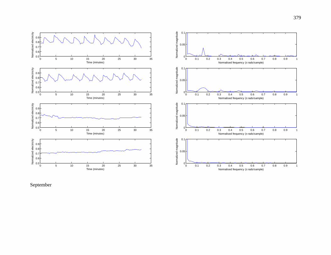
379

September

0 5 10 15 20 25 30 350.5

0.6

0.7

0.8

0.9

Time (minutes)

Nor

mal

ized

ele

ctric

ity

0 0.1 0.2 0.3 0.4 0.5 0.6 0.7 0.8 0.9 10

0.05

0.1


Nor

mal

ized

mag

nitu

de

0 5 10 15 20 25 30 350.5

0.6

0.7

0.8

0.9

Time (minutes)

Nor

mal

ized

ele

ctric

ity

0 0.1 0.2 0.3 0.4 0.5 0.6 0.7 0.8 0.9 10

0.05

0.1


Nor

mal

ized

mag

nitu

de

0 5 10 15 20 25 30 350.5

0.6

0.7

0.8

0.9

Time (minutes)

Nor

mal

ized

ele

ctric

ity

0 0.1 0.2 0.3 0.4 0.5 0.6 0.7 0.8 0.9 10

0.05

0.1


Nor

mal

ized

mag

nitu

de

0 5 10 15 20 25 30 350.5

0.6

0.7

0.8

0.9

Time (minutes)

Nor

mal

ized

ele

ctric

ity

0 0.1 0.2 0.3 0.4 0.5 0.6 0.7 0.8 0.9 10

0.05

0.1


Nor

mal

ized

mag

nitu

de

380

October

0 5 10 15 20 25 30 350.5

0.6

0.7

0.8

0.9

Time (minutes)

Nor

mal

ized

ele

ctric

ity

0 0.1 0.2 0.3 0.4 0.5 0.6 0.7 0.8 0.9 10

0.05

0.1


Nor

mal

ized

mag

nitu

de

0 5 10 15 20 25 30 350.5

0.6

0.7

0.8

0.9

Time (minutes)

Nor

mal

ized

ele

ctric

ity

0 0.1 0.2 0.3 0.4 0.5 0.6 0.7 0.8 0.9 10

0.05

0.1


Nor

mal

ized

mag

nitu

de

0 5 10 15 20 25 30 350.5

0.6

0.7

0.8

0.9

Time (minutes)

Nor

mal

ized

ele

ctric

ity

0 0.1 0.2 0.3 0.4 0.5 0.6 0.7 0.8 0.9 10

0.05

0.1


Nor

mal

ized

mag

nitu

de

0 5 10 15 20 25 30 350.5

0.6

0.7

0.8

0.9

Time (minutes)

Nor

mal

ized

ele

ctric

ity

0 0.1 0.2 0.3 0.4 0.5 0.6 0.7 0.8 0.9 10

0.05

0.1


Nor

mal

ized

mag

nitu

de

381

November

0 5 10 15 20 25 30 350.5

0.6

0.7

0.8

0.9

Time (minutes)

Nor

mal

ized

ele

ctric

ity

0 0.1 0.2 0.3 0.4 0.5 0.6 0.7 0.8 0.9 10

0.05

0.1


Nor

mal

ized

mag

nitu

de

0 5 10 15 20 25 30 350.5

0.6

0.7

0.8

0.9

Time (minutes)

Nor

mal

ized

ele

ctric

ity

0 0.1 0.2 0.3 0.4 0.5 0.6 0.7 0.8 0.9 10

0.05

0.1


Nor

mal

ized

mag

nitu

de

0 5 10 15 20 25 30 350.5

0.6

0.7

0.8

0.9

Time (minutes)

Nor

mal

ized

ele

ctric

ity

0 0.1 0.2 0.3 0.4 0.5 0.6 0.7 0.8 0.9 10

0.05

0.1


Nor

mal

ized

mag

nitu

de

0 5 10 15 20 25 30 350.5

0.6

0.7

0.8

0.9

Time (minutes)

Nor

mal

ized

ele

ctric

ity

0 0.1 0.2 0.3 0.4 0.5 0.6 0.7 0.8 0.9 10

0.05

0.1


Nor

mal

ized

mag

nitu

de

382

December

0 5 10 15 20 25 30 350.5

0.6

0.7

0.8

0.9

Time (minutes)

Nor

mal

ized

ele

ctric

ity

0 0.1 0.2 0.3 0.4 0.5 0.6 0.7 0.8 0.9 10

0.05

0.1


Nor

mal

ized

mag

nitu

de

0 5 10 15 20 25 30 350.5

0.6

0.7

0.8

0.9

Time (minutes)

Nor

mal

ized

ele

ctric

ity

0 0.1 0.2 0.3 0.4 0.5 0.6 0.7 0.8 0.9 10

0.05

0.1


Nor

mal

ized

mag

nitu

de

0 5 10 15 20 25 30 350.5

0.6

0.7

0.8

0.9

Time (minutes)

Nor

mal

ized

ele

ctric

ity

0 0.1 0.2 0.3 0.4 0.5 0.6 0.7 0.8 0.9 10

0.05

0.1


Nor

mal

ized

mag

nitu

de

0 5 10 15 20 25 30 350.5

0.6

0.7

0.8

0.9

Time (minutes)

Nor

mal

ized

ele

ctric

ity

0 0.1 0.2 0.3 0.4 0.5 0.6 0.7 0.8 0.9 10

0.05

0.1


Nor

mal

ized

mag

nitu

de

383

Appendix B – Summary of results from weekly data analyzed from all

months (aggregated electricity signal, probability of hoist operation,

filtered signal after extracting hoist electricity use, and hoist electricity

consumption)

384

January


0.5

1

Nor

mal

ized

ele

ctric

ity (k

Wh)



-1

0

1

Pro

babi

lty o

f hoi

st ru

nnin

g


0.5

1

Filtered signal electricity use: 95.8723 % of total electricity

Nor

mal

ized

ele

ctric

ity (k

Wh)

Jan 19 Jan 20 Jan 21 Jan 22 Jan 23 Jan 24 Jan 25 Jan 26-0.2

0

0.2

0.4

0.6

0.8Hoist electricity use: 4.1277 % of total electricity

Nor

mal

ized

ele

ctric

ity (k

Wh)

385

February

Feb 16 Feb 17 Feb 18 Feb 19 Feb 20 Feb 21 Feb 22 Feb 23

0.4

0.6

0.8

1

Nor

mal

ized

ele

ctric

ity (k

Wh)



-0.500.51

Pro

babi

lty o

f hoi

st ru

nnin

g


0.5

1


Nor

mal

ized

ele

ctric

ity (k

Wh)

Feb 16 Feb 17 Feb 18 Feb 19 Feb 20 Feb 21 Feb 22 Feb 23-0.2

0

0.2

0.4

0.6


Nor

mal

ized

ele

ctric

ity (k

Wh)

386

March

Mar 23 Mar 24 Mar 25 Mar 26 Mar 27 Mar 28 Mar 29 Mar 30

0.4

0.6

0.8

1

Nor

mal

ized

ele

ctric

ity (k

Wh)



-0.500.51

Pro

babi

lty o

f hoi

st ru

nnin

g


0.5

1


Nor

mal

ized

ele

ctric

ity (k

Wh)

Mar 23 Mar 24 Mar 25 Mar 26 Mar 27 Mar 28 Mar 29 Mar 30-0.2

0

0.2

0.4

0.6


Nor

mal

ized

ele

ctric

ity (k

Wh)

387

April

May 18 May 19 May 20 May 21 May 22 May 23 May 24 May 25

0.4

0.6

0.8

1

Nor

mal

ized

ele

ctric

ity (k

Wh)



-0.500.51

Pro

babi

lty o

f hoi

st ru

nnin

g


0.5

1


Nor

mal

ized

ele

ctric

ity (k

Wh)

May 18 May 19 May 20 May 21 May 22 May 23 May 24 May 25-0.2

0

0.2

0.4

0.6


Nor

mal

ized

ele

ctric

ity (k

Wh)

388

May


0.4

0.6

0.8

1

Nor

mal

ized

ele

ctric

ity (k

Wh)



-0.500.51

Pro

babi

lty o

f hoi

st ru

nnin

g


0.5

1


Nor

mal

ized

ele

ctric

ity (k

Wh)

May 18 May 19 May 20 May 21 May 22 May 23 May 24 May 25-0.2

0

0.2

0.4

0.6


Nor

mal

ized

ele

ctric

ity (k

Wh)

389

June

Jun 15 Jun 16 Jun 17 Jun 18 Jun 19 Jun 20 Jun 21 Jun 22

0.4

0.6

0.8

1

Nor

mal

ized

ele

ctric

ity (k

Wh)



-0.500.51

Pro

babi

lty o

f hoi

st ru

nnin

g


0.5

1


Nor

mal

ized

ele

ctric

ity (k

Wh)

Jun 15 Jun 16 Jun 17 Jun 18 Jun 19 Jun 20 Jun 21 Jun 22-0.2

0

0.2

0.4

0.6


Nor

mal

ized

ele

ctric

ity (k

Wh)

390

July

Jul 06 Jul 07 Jul 08 Jul 09 Jul 10 Jul 11 Jul 12 Jul 13

0.5

1

Nor

mal

ized

ele

ctric

ity (k

Wh)



-1

0

1

Pro

babi

lty o

f hoi

st ru

nnin

g


0.5

1


Nor

mal

ized

ele

ctric

ity (k

Wh)

Jul 06 Jul 07 Jul 08 Jul 09 Jul 10 Jul 11 Jul 12 Jul 13-0.2

0

0.2

0.4

0.6


Nor

mal

ized

ele

ctric

ity (k

Wh)

391

August

Aug 10 Aug 11 Aug 12 Aug 13 Aug 14 Aug 15 Aug 16 Aug 17

0.4

0.6

0.8

1

Nor

mal

ized

ele

ctric

ity (k

Wh)



-0.500.51

Pro

babi

lty o

f hoi

st ru

nnin

g


0.5

1


Nor

mal

ized

ele

ctric

ity (k

Wh)

Aug 10 Aug 11 Aug 12 Aug 13 Aug 14 Aug 15 Aug 16 Aug 17-0.2

0

0.2

0.4

0.6


Nor

mal

ized

ele

ctric

ity (k

Wh)

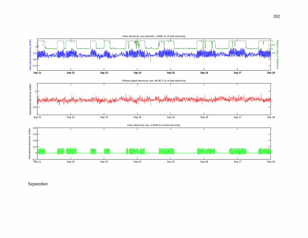
392

September

Sep 21 Sep 22 Sep 23 Sep 24 Sep 25 Sep 26 Sep 27 Sep 28

0.4

0.6

0.8

1

Nor

mal

ized

ele

ctric

ity (k

Wh)



-0.500.51

Pro

babi

lty o

f hoi

st ru

nnin

g


0.5

1


Nor

mal

ized

ele

ctric

ity (k

Wh)

Sep 21 Sep 22 Sep 23 Sep 24 Sep 25 Sep 26 Sep 27 Sep 28-0.2

0

0.2

0.4

0.6


Nor

mal

ized

ele

ctric

ity (k

Wh)

393

October

Oct 19 Oct 20 Oct 21 Oct 22 Oct 23 Oct 24 Oct 25 Oct 26

0.4

0.6

0.8

1

Nor

mal

ized

ele

ctric

ity (k

Wh)



-0.500.51

Pro

babi

lty o

f hoi

st ru

nnin

g


0.5

1


Nor

mal

ized

ele

ctric

ity (k

Wh)

Oct 19 Oct 20 Oct 21 Oct 22 Oct 23 Oct 24 Oct 25 Oct 26-0.2

0

0.2

0.4

0.6


Nor

mal

ized

ele

ctric

ity (k

Wh)

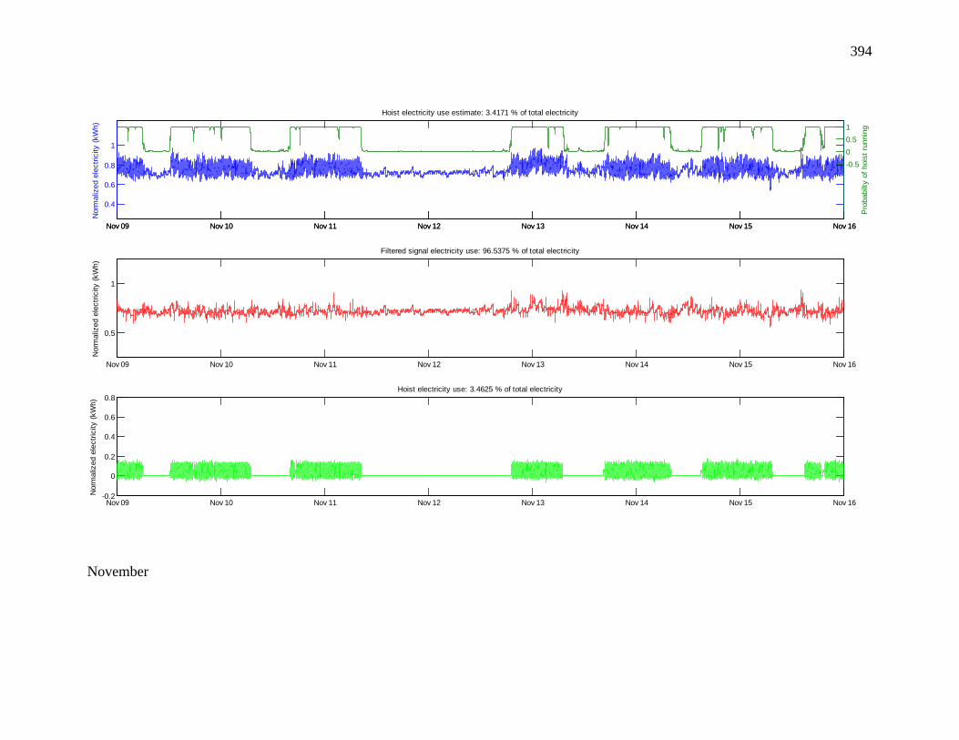
394

November

Nov 09 Nov 10 Nov 11 Nov 12 Nov 13 Nov 14 Nov 15 Nov 16

0.4

0.6

0.8

1

Nor

mal

ized

ele

ctric

ity (k

Wh)



-0.500.51

Pro

babi

lty o

f hoi

st ru

nnin

g


0.5

1


Nor

mal

ized

ele

ctric

ity (k

Wh)

Nov 09 Nov 10 Nov 11 Nov 12 Nov 13 Nov 14 Nov 15 Nov 16-0.2

0

0.2

0.4

0.6


Nor

mal

ized

ele

ctric

ity (k

Wh)

395

December

Dec 14 Dec 15 Dec 16 Dec 17 Dec 18 Dec 19 Dec 20 Dec 21

0.4

0.6

0.8

1

Nor

mal

ized

ele

ctric

ity (k

Wh)



-0.500.51

Pro

babi

lty o

f hoi

st ru

nnin

g


0.5

1


Nor

mal

ized

ele

ctric

ity (k

Wh)

Dec 14 Dec 15 Dec 16 Dec 17 Dec 18 Dec 19 Dec 20 Dec 21-0.2

0

0.2

0.4

0.6


Nor

mal

ized

ele

ctric

ity (k

Wh)

396

Holidays


0.60.650.70.750.8

0.850.90.951

Nor

mal

ized

ele

ctric

ity (k

Wh)



-0.6-0.4-0.200.20.40.60.81

Pro

babi

lty o

f hoi

st ru

nnin

g


0.5

1


Nor

mal

ized

ele

ctric

ity (k

Wh)

Dec 21 Dec 22 Dec 23 Dec 24 Dec 25 Dec 26 Dec 27 Dec 28-0.2

0

0.2

0.4

0.6


Nor

mal

ized

ele

ctric

ity (k

Wh)

397

Shutdown


0.4

0.6

0.8

1

Nor

mal

ized

ele

ctric

ity (k

Wh)



00.20.40.60.81

Pro

babi

lty o

f hoi

st ru

nnin

g


0.5

1


Nor

mal

ized

ele

ctric

ity (k

Wh)

Jul 15 Jul 16 Jul 17 Jul 18 Jul 19 Jul 20 Jul 21 Jul 22-0.2

0

0.2

0.4

0.6


Nor

mal

ized

ele

ctric

ity (k

Wh)

An improved energy management methodology for the mining ...

Documents

Transcript of An improved energy management methodology for the mining ...