An implicit and explicit solver for contact problems

An implicit and explicit solver for contact problems

J.H. Schutte, J.F. Dannenberg, Y.H. Wijnant and A. de BoerUniversity of Twente, Institute of Mechanics, Processes, and Control- Twente,Structural Dynamics and Acoustics group,P.O. Box 217, 7500 AE Enschede, The Netherlandse-mail: [email protected]

AbstractThe interaction of rolling tyres with road surfaces is one of the major contributions to road traffic noise. Thegeneration mechanisms of tyre/road noise are usually separated in structure borne and airborne noise. Inboth mechanisms the contact zone is important. In order to reduce tyre/road noise at the source, accurate(numerical) prediction models are needed. For accurate results, the tyre has to be modelled by a three-dimensional finite element model, accounting for complex rubber material behaviour, tread profiles and adetailed tyre construction. A dynamic analysis of a tyre in contact can then becarried out in the time domain.The Structural Dynamics and Acoustics group of the University of Twentehas developed an alternativecontact solver. The solver, in which the contact condition is always satisfied, is successfully applied to animplicit and explicit three-dimensional finite element model. As a consequence there is no need for contactelements or contact parameters. The finite element model is valid for large translations and rotations, inwhich different material models and friction models can be added. This paper explains the solver for animplicit and explicit scheme and presents some examples. In one of the examplesa deformable rubber ringis modelled, which is rolling on a rigid surface at a slip angle. The results are compared to the finite elementpackage Abaqus. The examples show the robustness and potential of thealgorithm.

1 Introduction

In modern society, traffic noise has become an important issue for mental health. A significant contributor tothis noise pollution is tyre/road noise, which is caused by the interaction between tyre and road surface. Thenoise generating mechanisms have been identified, although there is discussion on the relative importanceof these mechanisms. From experiments, it is known that spectra of tyre/road noise display a broad peaksomewhere in the range of 500–2000 Hz [13].

The calculation of tyre/road noise is usually performed by means of two separate steps. First thetyre vibra-tionsare calculated which serve then as an input for thesound radiationmodel. The numerical tyre vibrationmodels range from analytical models, where the tyre vibrations are modelled by means of a ring, shell orplate [8], to numerical models based on finite elements [12]. The sound radiation can be based on analyticalmultipole models [9] and numerical models based on finite elements or boundary elements. An alternativegroup of tyre/road noise models are the statistical and hybrid models [10]. Since these models are empiri-cally based, the accuracy is limited by the quality of the input data, and in a sense, is not predictive. Thispaper will focus on thenumericaltyre vibration models only.

Examples of tyre vibration models can be found in literature. Kropp,et al. [11, 21, 1] modelled the vibrationsof a multilayered plate using a three-dimensional nonlinear contact model. Nackenhorst, Brinkmeier,et al.[12, 3] used the Arbitrary Lagrangian Eulerian (ALE) method and complexeigenfrequencies to model thetyre vibrations. A recent overview on the use of finite elements of rolling tyres is given by Ghoreishy [6].

To quantitatively study the influence of the tyre on tyre/road noise, detailed finite element models are needed.

4081

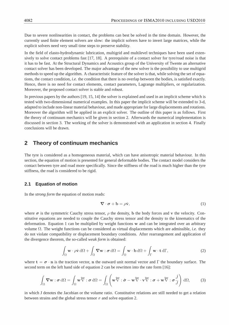
Due to severe nonlinearities in contact, the problems can best be solved in thetime domain. However, thecurrently used finite element solvers are slow: the implicit solvers have to invert large matrices, while theexplicit solvers need very small time steps to preserve stability.

In the field of elasto-hydrodynamic lubrication, multigrid and multilevel techniques have been used exten-sively to solve contact problems fast [17, 18]. A prerequisite of a contact solver for tyre/road noise is thatit has to be fast. At the Structural Dynamics and Acoustics group of the University of Twente an alternativecontact solver has been developed. The major advantage of the new solver is the possibility to use multigridmethods to speed up the algorithm. A characteristic feature of the solver is that,while solving the set of equa-tions, the contact condition,i.e. the condition that there is no overlap between the bodies, is satisfied exactly.Hence, there is no need for contact elements, contact parameters, Lagrange multipliers, or regularization.Moreover, the proposed contact solver is stable and robust.

In previous papers by the authors [19, 15, 14] the solver is explained and used in an implicit scheme which istested with two-dimensional numerical examples. In this paper the implicit scheme will be extended to 3-d,adapted to include non-linear material behaviour, and made appropriate for large displacements and rotations.Moreover the algorithm will be applied in an explicit solver. The outline of this paper is as follows. Firstthe theory of continuum mechanics will be given in section 2. Afterwards thenumerical implementation isdiscussed in section 3. The working of the solver is demonstrated with an application in section 4. Finallyconclusions will be drawn.

2 Theory of continuum mechanics

The tyre is considered as a homogeneous material, which can have anisotropic material behaviour. In thissection, the equation of motion is presented for general deformable bodies. The contact model considers thecontact between tyre and road more specifically. Since the stiffness of theroad is much higher than the tyrestiffness, the road is considered to be rigid.

2.1 Equation of motion

In thestrong formthe equation of motion reads:

∇ · σ + b = ρv, (1)

whereσ is the symmetric Cauchy stress tensor,ρ the density,b the body forces andv the velocity. Con-stitutive equations are needed to couple the Cauchy stress tensor and the density to the kinematics of thedeformation. Equation 1 can be multiplied by weight functionsw and can be integrated over an arbitraryvolumeΩ. The weight functions can be considered as virtual displacements which are admissible,i.e. theydo not violate compatibility or displacement boundary conditions. After rearrangement and application ofthe divergence theorem, the so-calledweak formis obtained:∫

Ωw · ρv dΩ +

∫Ω

∇w : σ dΩ =∫

Ωw · b dΩ +

∫Γw · t dΓ, (2)

wheret = σ · n is the traction vector,n the outward unit normal vector andΓ the boundary surface. Thesecond term on the left hand side of equation 2 can be rewritten into the rate form [16]:∫

Ω∇w : σ dΩ =

∫Ω

w←−∇ : σ dΩ =

∫Ω

(w←−∇ : σ −w

←−∇ · v←−∇ : σ + w←−∇ : σ

J

J

)dΩ, (3)

in which J denotes the Jacobian or the volume ratio. Constitutive relations are still needed to get a relationbetween strains and the global stress tensorσ and solve equation 2.

4082 PROCEEDINGS OF ISMA2010 INCLUDING USD2010

Γ

Ω

n

tN

t

tT

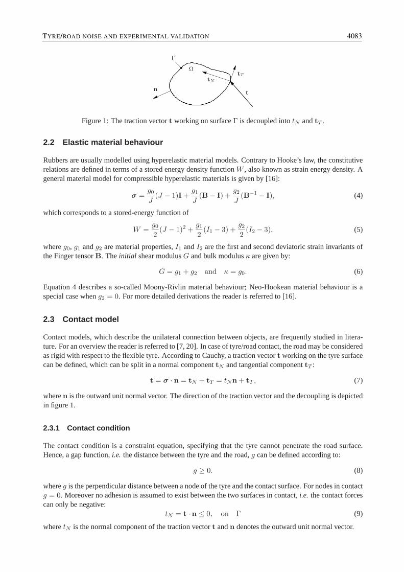
Figure 1: The traction vectort working on surfaceΓ is decoupled intotN andtT .

2.2 Elastic material behaviour

Rubbers are usually modelled using hyperelastic material models. Contrary toHooke’s law, the constitutiverelations are defined in terms of a stored energy density functionW , also known as strain energy density. Ageneral material model for compressible hyperelastic materials is given by [16]:

σ =g0

J(J − 1)I +

g1

J(B− I) +

g2

J(B−1 − I), (4)

which corresponds to a stored-energy function of

W =g0

2(J − 1)2 +

g1

2(I1 − 3) +

g2

2(I2 − 3), (5)

whereg0, g1 andg2 are material properties,I1 andI2 are the first and second deviatoric strain invariants ofthe Finger tensorB. Theinitial shear modulusG and bulk modulusκ are given by:

G = g1 + g2 and κ = g0. (6)

Equation 4 describes a so-called Moony-Rivlin material behaviour; Neo-Hookean material behaviour is aspecial case wheng2 = 0. For more detailed derivations the reader is referred to [16].

2.3 Contact model

Contact models, which describe the unilateral connection between objects,are frequently studied in litera-ture. For an overview the reader is referred to [7, 20]. In case of tyre/road contact, the road may be consideredas rigid with respect to the flexible tyre. According to Cauchy, a traction vector t working on the tyre surfacecan be defined, which can be split in a normal componenttN and tangential componenttT :

t = σ · n = tN + tT = tNn + tT , (7)

wheren is the outward unit normal vector. The direction of the traction vector and thedecoupling is depictedin figure 1.

2.3.1 Contact condition

The contact condition is a constraint equation, specifying that the tyre cannot penetrate the road surface.Hence, a gap function,i.e. the distance between the tyre and the road,g can be defined according to:

g ≥ 0. (8)

whereg is the perpendicular distance between a node of the tyre and the contact surface. For nodes in contactg = 0. Moreover no adhesion is assumed to exist between the two surfaces in contact,i.e. the contact forcescan only be negative:

tN = t · n ≤ 0, on Γ (9)

wheretN is the normal component of the traction vectort andn denotes the outward unit normal vector.

TYRE/ROAD NOISE AND EXPERIMENTAL VALIDATION 4083

2.3.2 Friction model

When the tyre is in contact with the road, the friction model determines whether the tyre sticks or slips.Coulomb’s friction law states that the tangential traction is limited by the coefficientof friction times thenormal traction:

|tT | ≤ µ|tN |, on Γ (10)

whereµ is the friction coefficient and| · | the length of the vector. Points onΓ that fulfill equation (10),stick to the surface and point that do not, slip along the surface with|tT | = µ|tN |. For frictionless contact,µ = 0. Coulomb’s friction model is used in the contact algorithm because of its simplicityand the existenceof analytical solutions, but the contact algorithm is not restricted to this friction model. The static frictionmodels, like viscous friction and Stribeck friction, or more advanced dynamicmodels can be applied as well.

3 Numerical implementation

In section 2 the equation of motion has been formulated as a partial differential equation. In this section thedifferential equation will be discretized. Additionally constitutive relations and boundary conditions, givenby the contact model, are applied. The contact algorithm is used in an implicit and explicit scheme. Bothschemes will be discussed and the required integration methods will be given.

The interaction between tyre and road surface is inherently non-linear, and has to be solved in the time do-main. The equation of motion will be solved using the contact model. The finite element method, integrationmethods and algorithms are discussed in literature extensively, seee.g. [2, 4, 22].

3.1 Finite element method

In order to solve the problem numerically, the continuous domain is discretizedby dividing it in a numberof elements. Following the approach by Galerkin, the weight functionsw are chosen equal to the shapefunctionsN. For solving contact problems it is preferable to use linear shape functions. Substituting theshape functions into equation 2 leads to a discrete problem:

Mu + fint(u) = fext, (11)

where

M =∫

ΩNTρN dΩ, (12)

fint(u) =∫

ΩBTσ dΩ, (13)

fext =∫

ΩNTb dΩ +

∫ΓNTt dΓ, (14)

in which M is mass matrix,fint(u) the internal force vector (also referred to as stress divergence),fext

the external force vector,u the nodal displacement vector,N the shape functions, andB the derivative ofthe shape functions. For continuum elements the mass of each element remainsconstant by virtue of theconservation of mass. In subsequent sections, the contact forcesfcont are part of the external forces workingon the body.

3.2 Implicit scheme

In the implicit scheme, equation 11 is solved iteratively under appropriate initialconditions, where the dis-cretized contact model serves as a boundary condition. The solver comprises three main steps:


• The Newmark method is used for single-step time integration.

• The nonlinear equations are linearized using the Newton-Raphson method.

• Gauss-Seidel relaxation is used to fulfill the contact condition and friction model.

The characteristic of the solver is that the contact condition is satisfied during solving without the use ofLagrange multipliers or penalty functions. An overview of the steps of the implicit solver is given in fig-ure 2. Before discussing the flowchart, the appliedincremental strategywill be introduced briefly. The totalincrement in the displacement vector can be written as:

un+1 = un + ∆u, (15)

and the iterative increment by:∆uk+1 = ∆uk + δuk, (16)

where the subscriptn refers to the time step and the superscriptk the iteration number.

As shown in figure 2 we start with sufficient initial conditions and boundaryconditions. In the first stepthe algorithm calculates the internal and external forces,fint and fext respectively, according to the initialconfiguration.

The Newmark method is used to calculate an update when the time is increased by atime step∆t. Newmarkintegration methods are a family of one-step integration methods, using the current state and the state to becalculated [2, 22]. An update for the velocityu and accelerationu can be calculated by:

un+1 =1

β∆t2(un+1 − un −∆t un)−

(12β− 1)

un, (17)

un+1 =γ

β∆t(un+1 − un)−

(γ

β− 1)

un −∆t

(γ

2β− 1)

un, (18)

in which usuallyγ = 12 andβ = 1

4 . In case of severe nonlinearitiesmodifiedaverage constant accelerationcan be used to introduce numerical damping to the high frequency modes andpreserve stability.

In the predictor step the Newton-Raphson method is used to evaluate a linear equivalent of the nonlinearequation of motion. Equation 3 can be used to get a first order approximationof the internal forces whichuses a tangent stiffness matrixK:

fint n+1 = fint n + Kn∆u. (19)

Substitution of equations 17 and 18 into equation 11 leads to:(1

β∆t2M + Kn

)∆u = fext n+1 − fint n + M

(1

β∆tun +

[12β− 1]un

). (20)

The nonlinear equation of motion (equation 20) can be solved to get the iterative displacementδuk. Accord-ing to the Newton-Raphson process the increment is calculated by:

K∗δuk = −rk, (21)

where

K∗ =1

β∆t2M + K, (22)

andrk denotes the residual force vector. The iterations are stopped when the norm ofr is less than the normof fint: ‖r‖

‖fint‖ < εNR, (23)


where‖ · ‖ is the Euclidean orL2 norm andεNR is user-defined stop criterion of the Newton-Raphsoniteration. Solving equation 21 is rather straightforward for unconstrainedproblems where contact is omitted.Note that in constrained problemsr is a function of the external force in the current time stepfext n+1.

In the most inner loop, relaxation is used so solve equation 21, where the boundary conditions are taken intoaccount. For all nodes, it is evaluated if they are in contact or not. The displacement of a nodei, which isout of contact, is updated using:

δuk+1i = (1− ω)δuk

i +ω

K∗ii

−ri −i−1∑j=1

K∗ijδu

k+1j −

N∑j=i+1

K∗ijδu

kj

, (24)

whereN denotes the number of nodes and the parameterω can be used to improve stability. Whenω = 1 thescheme is equal to Gauss-Seidel relaxation. Ifω < 1, the so-called underrelaxation can improve the stabilityand, ifω > 1, overrelaxation can be used to speed up on the other hand. The contactcondition is evaluatedfor the updated displacementun+1. If g < 0, nodei is apparently penetrating the surface. The node is putback on the surface (g = 0) and the external forces are updated. If nodei is not in contact (g ≥ 0), the updatemay be applied and the process continues for nodei + 1.

For nodesin contactthe contact force (fcont = fN + fT ) is calculated and evaluated. If a normal contactforce fN < 0 is found, which would imply that the node is attracted by the surface, the nodeis releasedfrom contact and the contact force is put to zero (fcont = 0). For the nodes which remain in contact thetangential forces are evaluated according to Coulomb’s friction model (|fT | ≤ µ|fN |). If necessary, slip canbe applied and the displacement, velocity and acceleration can be updated. The described process continuesuntil convergence is reached for all nodes. The Euclidean norm of theresidualr∗ = r + K∗δu can be usedas stop criterion:

‖r∗‖ < εGS, (25)

whereεGS is the stop criterion for the Gauss-Seidel relaxation. For every new time step, the same strategy isfollowed until the last time step has been reached (n = nmax). More information about the implicit schemeand some applications can be found in [5].

3.3 Explicit scheme

In the explicit scheme the contact algorithm is applied in an explicit Newmark scheme (β = 0, γ = 12 ). The

scheme shows similarities with the general contact algorithm, which is implemented in the finite elementpackage Abaqus/Explicit. Equation 11 can be written as:

u = M−1 (fext − fint(u)) = M−1f . (26)

Applying the time integration formulas, the velocity and displacement can be calculated using constant timeincrements∆t:

un+ 12

= un− 12

+ ∆t un (27)

un+1 = un + ∆t un+ 12, (28)

where the velocity is lagging by half a time step. The explicit Newmark scheme caneasily be recognized asa central difference scheme. A big advantage is the use of a diagonal mass matrix, by which the calculationof u is trivial. Sincefint(u) andfext are dependent on the displacement, the scheme is not fully explicit. Theexplicit central difference scheme is conditionally stable. Hence the time increment∆t must be chosen lessthan a critical time step∆tcrit:

∆tcrit =2

ωmax, (29)

whereωmax denotes the maximum eigenfrequency of the linear system.


in contact? calculate

fN < 0

corrector

fcont = 0update

g < 0

for all nodes

g = 0 |fT ||fT |

initial conditions

results

=

correct

no

no

no

no

no

no

non = nmax

not in contact in contact

predictor

‖r∗‖ < εGS

‖r‖‖fint‖ < εNR

fcont

tn + ∆t

u, u, u

u, u, u

>yesyes

yes

yes

yes

yes

yes

µ|fN | µ|fN |

Figure 2: Flowchart of the solver with an implicit scheme.


An overview of the explicit scheme is given in figure 3. For the first time step,the internal and externalforces and the accelerations are determined. From this information updatedvalues for the displacement andacceleration can be calculated. The algorithm evaluates which nodes are incontact. For the nodes in contact,contact forces are applied and displacements, velocities and accelerations are be updated. For all nodes, thecorrector calculates the new internal forces. The contact condition andslip criterion are evaluated and theaccelerations of the new step can be applied. In the energy balance instabilities can be found, which mayoccur even when the critical time step requirement is fulfilled [2].

4 Application

In the previous section the numerical implementation of the algorithm in an implicit andexplicit schemehave been discussed. In this section an application is given to show the performance of the solver. In theexamples a rubber ring will be considered. The results are compared to thefinite element package Abaqusand evaluated at the end.

4.1 Introduction to LAT-100

The Laboratory Abrasion and skid Tester 100 (LAT-100) is an apparatus which is able to measure the skid,traction, and wear resistance of (tread) rubber compounds with a disk which represents a road surface. Arubber sample is tested in the form of a small solid tyre which is rolling on the rotating disk, where the speed,slip angle, load and surface of the disk can be changed.

The small LAT-100 tyre can be used to validate the contact algorithm, since thegeometry is simple and thematerial uniform. An overview of the dimensions and directions are depicted infigure 4. The outer and innerradius areRout = 39 mm andRin = 17 mm, respectively and the width isw = 17.5 mm. The tyre is madeout of tread rubber with densityρ = 1100 kg/m3. It is modelled as a Neo-Hookean hyperelastic materialwith shear modulusG = 2.64 MPa and bulk modulusκ = 65.1 MPa. The inside of the tyre is supported bya rigid rim, which can be controlled by a forceF , a rotational velocity around they-axis θ, or a translationalvelocity u under slip angleα with respect to the positivex-axis. The finite element mesh consists of 880linear eight node hex elements. The rotating disk, on which the tyre is rolling, ismodelled as a flat rigidsurface.

The results are compared with the finite element package Abaqus. Where possible, the settings are keptthe same. In Abaqus/Standard the interaction between LAT-100 tyre and therigid surface is modelled as ahard contact using the (default) penalty method applied to surface-to-surface contact pairs. A basic Coulombfriction model is used in the tangential direction. In Abaqus/Explicit the general contact algorithm is used tomodel the normal contact behaviour.

4.2 Static loading

In the static simulation a compressive forceF = 300 N is working on the rim of the LAT-100 tyre. As aresult the rim axle translates 2.2 mm in negativez-direction. For the frictionless case the differences betweenthe implicit scheme and Abaqus are marginal, and are therefore not given.In figure 5 the contact forces areshown as calculated with the implicit scheme and Abaqus/Standard, depicted above and below, respectively.Differences can be found in the shear forces at the edges of the contact zone, in normal direction thesedifferences however are less pronounced.

4.3 Dynamic rolling

To perform the dynamic rolling simulations the explicit contact algorithm is used,and the results are com-pared to Abaqus/Explicit.


in contact?

un+1 = M−1fn+1

fN < 0

corrector fint

fcont = 0

energy balance

calculatefcont

|fT ||fT |

initial conditions

results

=

no

no

no

non = nmax

not in contact in contact

set first time step

updateu, u, u

>

tn+1 = tn + ∆t

yes

yes

yes

yes

un+ 12

= un− 12

+ ∆t un

µ|fN | µ|fN |

un+1 = un + ∆t un+ 12

Figure 3: Flowchart of the solver with an explicit scheme.


α

α

F

F

Rin

Rin

Rout

Rout

θ

θ

u

u

x

x

x

y

yz

z

Figure 4: Dimensions and directions for the LAT-100 test tyre.

0

5

10

15

20

25

(a) Normal force in N

0

2

4

6

8

(b) Shear force in N

Figure 5: Contact forces on the tyre after static compression on a rigid surface (µ = 1.0) for the implicitsolver (above) and Abaqus/Standard (below).


0

5

10

15

20

25

(a) Normal force in N

0

5

10

15

(b) Shear force in N

Figure 6: Contact forces on the tyre during rolling on a rigid surface (µ = 1.0) for the explicit solver (above)and Abaqus/Explicit (below). The tyre is rolling in clockwise direction to the right.

4.3.1 Rolling in a straight line

At the start the LAT-100 test tyre is in a deformed shape, as obtained fromthe implicit scheme.1 In thedynamic simulation the rim axle is forced to translate with velocityu = 2.59 m/s at heightz = −2.2 mm,and forced to rotate withθ = 70 rad/s. A friction coefficientµ = 1.0 is assumed between the tyre and thesurface. After 0.1 s the contact forces are compared in figure 6. The tyre, which is in a deformed shape, isrolling in clockwise direction to the right. The main differences can be found inthe shear force distribution.Because the tyre is not rolling free,i.e. there is a nett moment around the rim axle, the shear forces increaseand depend significantly on the followed path. A small change in the boundary conditions results in largedifferences in shear forces.

4.3.2 Rolling under a large slip angle

In the second dynamic simulation the rim axle is forced to translate with velocityu = 2.687 m/s at a slipangleα = 45 deg and heightz = −2.2 mm, and forced to rotate withθ = 70 rad/s. A friction coefficientµ = 0.5 is applied. As a result the tyre deforms extremely while it slips along the surface. The contact zoneshifts towards the side, which is in contact first, as can be seen in figure 7.The results for rolling under alarge slip angle match very well with Abaqus, for both normal and shear forces. Instead of the normal forces,a view from behind of the deformed tyre is given in figure 7a.

4.4 Evaluation

The contact solver is successfully applied in an implicit and explicit scheme which is able to perform staticand dynamic simulations with rubber material and large deformations and rotations. In normal directionthe results are in good agreement with Abaqus. The main differences between the solver and Abaqus can befound in the tangential direction. These differences are more pronounced because of the relative coarse mesh.Since the correct modelling of shear forces is hard, both simulations can best be compared to experimentalresults. A main disadvantage of the scheme is the calculation time, which is more thanan order higherthan Abaqus. At this moment the simulation of large finite element models is still a challenging task. Theimplementation of multigrid techniques can speed up the solver. In the explicit scheme the corrector step,

1In Abaqus/Explicit the LAT-100 test tyre is put in contact during the explicitcalculation using a smooth step.


(a) Deformed shape viewed from be-hind for explicit solver (right) andAbaqus/Explicit (left).

0

5

10

15

20

25

30

(b) Shear force in N for explicit solver (above) andAbaqus/Explicit (left)

Figure 7: Deformed shape of the tyre during rolling under a 45 degree slipangle (µ = 0.5). The tyre isrolling in clockwise direction.

which calculates the internal forces and currently takes most of the work,can be accelerated. Nevertheless,the solver behaves very robust and can easily adapted by the user. Therefore the algorithm has great potential.

5 Conclusions

A new contact solver has been developed and is successfully applied in an implicit and explicit three-dimensional finite element scheme. In the solver the contact condition is always satisfied, so there is noneed for contact elements or contact parameters. The finite element model isvalid for large translationsand rotations, in which different material models and friction models can be added. A small rubber tyre ismodelled statically and dynamically, and the results are compared with the finite element package Abaqus.Globally the solver predicts the same deformations as Abaqus. In normal direction the forces agree well,while there are some differences in the calculated shear forces. At the time of writing the calculation timeof the solvers is still more than an order of magnitude larger than the Abaqus simulations. The exampleshowever show the working, the robustness and the potential of the algorithm.

Future research can aim at an experimental study on the contact zone witha special focus on the shearforces. In the LAT-100 experimental test setup the forces can be measured and compared to the simulations.The simulations on the other hand can be improved by using finer meshes. Thesolver, which is currentlyprogrammed in MATLAB, can be rewritten in C or Fortran. Moreover multigrid techniques can be used tospeed up the implicit scheme. In the explicit scheme the calculation of the internalforces, which takes upmost of the calculation time, can be accelerated.

Acknowledgements

The support of TNO and Apollo Vredestein within this CCAR project is gratefully acknowledged by theauthors.


References

[1] P.B.U. Andersson, W. Kropp,Time domain contact model for tyre/road interaction including nonlinearcontact stiffness due to small-scale roughness, Journal of Sound and Vibration, Vol. 318 (2008), pp.296–312.

[2] T. Belytschko, W.K. Liu, B. Moran,Nonlinear Finite Elements for Continua and Structures, first edi-tion, John Wiley & Sons (2000).

[3] M. Brinkmeier, U. Nackenhorst, S. Petersen, O. von Estorff,A finite element approach for the simula-tion of tire rolling noise, Journal of Sound and Vibration, Vol. 309 (2008), pp. 20–39.

[4] R.D. Cook, D.S. Malkus, M.E. Plesha, R.J. Witt,Concepts and Applications of Finite Element Analysis,fourth edition, John Wiley & Sons (2002), ISBN 0470088214.

[5] J.F. Dannenberg,An implicit and explicit finite element solver for tyre/road contact, Master’s thesis,University of Twente, Enschede, The Netherlands (2009).

[6] M.H.Z. Ghoreishy,A state of the art review of the finite element modelling of rolling tyres, IranianPolymer Journal, Vol. 17, No. 8 (2008), pp. 571–597.

[7] G. Kloosterman,Contact Methods in Finite Element Simulations, Ph.D. thesis, University of Twente,Enschede, The Netherlands (2002).

[8] W. Kropp, Ein Modell zur Beschreibung des Rollgerausches eines unprofilierten Gurtelreifens aufrauher Strassenoberflache, Ph.D. thesis, Institut fur Technische Akustik, Berlin, Germany (1992).

[9] W. Kropp, F.-X. Becot, S. Barrelet,On the sound radiation from tyres, Acustica, Vol. 86, No. 5 (2000),pp. 769–779.

[10] A.H.W.M. Kuijpers,Further analysis of the Sperenberg data, Towards a better understanding of pro-cesses influencing tyre/road noise, Technical Report M+P.MVM.99.3.1, M+P Raadgevende ingenieursbv, ’s-Hertogenbosch, The Netherlands (2001).

[11] K. Larsson,Modelling of Dynamic Contact – Exemplified on the Tyre/Road Interaction, Ph.D. thesis,Chalmers University of Technology, Goteborg, Sweden (2002).

[12] U. Nackenhorst,The ALE-formulation of bodies in rolling contact – theoretical foundations and finiteelement approach, Computer Methods in Applied Mechanics and Engineering, Vol. 193 (2004), pp.4299–4322.

[13] U. Sandberg, J.A. Ejsmont,Tyre/Road Noise Reference Book, INFORMEX, Harg, SE-59040 Kisa,Sweden (2002).

[14] J.H. Schutte, Y.H. Wijnant, A. de Boer,A contact solver suitable for finite elements, in Proceedings ofISMA2008, Leuven, Belgium (2008).

[15] J.H. Schutte, Y.H. Wijnant, A. de Boer,A contact solver suitable for tyre/road noise analysis, in Pro-ceedings of Acoustics’08, Paris, France (2008).

[16] R.H.W. ten Thije,Finite Element Simulations of Laminated Composite Forming Processes, Ph.D. thesis,University of Twente, Enschede, The Netherlands (2007).

[17] C.H. Venner,Multilevel solvers for the EHL line and point contact problems, Ph.D. thesis, Universityof Twente, Enschede, The Netherlands (1991).


[18] Y.H. Wijnant,Contact Dynamics in the field of Elastohydrodynamic Lubrication, Ph.D. thesis, Univer-sity of Twente, Enschede, The Netherlands (1998).

[19] Y.H. Wijnant, A. de Boer,A new approach to model tyre/road contact, in Proceedings of ISMA2006,Leuven, Belgium (2006).

[20] P. Wriggers,Computational Contact Mechanics, John Wiley & Sons (2002).

[21] F. Wullens, W. Kropp,Wave content of the vibration field of a rolling tyre, Acta Acustica united withAcustica, Vol. 93 (2007), pp. 48–56.

[22] O.C. Zienkiewic, R.L. Taylor,The Finite Element Method, Volume 2: Solid mechanics, fifth edition,Butterworth-Heinemann (2000).


An implicit and explicit solver for contact problems

Documents

Transcript of An implicit and explicit solver for contact problems