An Implementation of the Equipment and Techniques used by

The Beatles at Abbey Road during the 1960s

by

Jacob Miller

Thesis Advisor: Cosette Collier

A thesis presented to the Honors College of Middle Tennessee State University in partial

fulfillment of the requirements for graduation from the University Honors College

Spring 2018

An Implementation of the Equipment and Techniques used by

The Beatles at Abbey Road during the 1960s

Jacob Miller

APPROVED:

______________________________ Professor Cosette Collier Recording Industry

______________________________ Beverly Keel Recording Industry

______________________________ Alton Dellinger

Recording Industry

______________________________ Dean John Vile University Honors College Dean

!ii

!iii

Abstract

This project consisted of three distinct, but interrelated components: (1) research into the

REDD series of equipment, particularly the passive equalizer design, used at Abbey

Road, (2) documentation of Beatles’ recording sessions, including layout, equipment

used, and how the equipment was implemented, and (3) production of new sound

recordings on analog tape. The over-arching goal was to mimic conditions of the Abbey

Road as closely as possible, including microphone positions, instruments used, duration

of sessions, and other variables to produce recordings in the style of The Beatles. To

better capture this distinctive style, I also used several effects frequently used by the

Beatles, including varispeed, half speed overdubbing, and repeat echo. Thus, I generated

an extended play album consisting of three analog songs: “Neon Sunrise,” “Words,” and

“How the Tune Goes."

!iv

Table of Contents

Title Page .……………………………………………………………………………… i

Signature Page …….………………………………………………………………….. ii

Abstract .…….…………………………………………………………………….……. iv

List of Tables……………………………………………………………………….…... vi

List of Figures…….….………………..……………………………………………….. vii

Introduction ..…..…….………………………………………………………………… 1

Approach and Methods………………………………………………………………… 4

REDD Design and Signal Flow ………..……………………………………………… 6 Designing a Balanced Bridged “T” Pad ………………………………………………… 7 Designing a Variable Balanced Bridged “T” Attenuator ………………..………………. 8 Three Way Selector …………………………………………………………………….. 17 REDD.47 Preamp ……………………………………………………………….……… 23 Designing the REDD Tone Controls …………………………………………………… 24 The Stereophonic System ………………………………………………………………. 46 Designing a Power Supply Suitable for the REDD.47 Preamps ……………………….. 47

Product: Sound Recordings ………………………………………………………….. 49 Effects ………………………………………………………………………………….. 49 How The Tune Goes …………………………………………………………………… 53 Neon Sunrise …………………………………………………………………………… 56 Words ………………………………………………………………………………….. 58 Post Production ………………………………………………………………………… 60

References …………………………………………………………………………….. 64

!v

List of Tables

Table 1. K Values for Variable Bridged “T” Attenuator …………………………… 12

Table 2. Frequency of Half Pad Loss ………………………………………………… 21

Table 3. Equations for Figures 13, 14, & 15 ………………………………………… 26

Table 4. Design Elements for “Pop” Filter High Boost …………………………….. 32

Table 5. Design Elements for “Pop” Filter Low Boost …………………………..…. 37

Table 6. Design Elements for “Pop" Filter High Cut ……………………………… 41

Table 7. Design Elements for “Pop” Filter Low Cut ……………………………….. 44

Table 8. “How The Tune Goes” Tracks ……………………………………………… 53

Table 9. “Neon Sunrise” Tracks ……………………………………………………… 56

Table 10. “Words” Tracks ……………………………………………………………. 60

!vi

List of Figures

Figure 1. Bridged “T” Pad ……………………………………………………………. 8

Figure 2. 20dB Bridged “T” Pad ……………………………………………………… 9

Figure 3. Balanced Bridged “T” Pad ……………………………………………….. 10

Figure 4. 20dB Balanced Bridged “T” Pad …………………………………………. 10

Figure 5. 30dB Variable Bridged “T” Pad …………………………………………... 15

Figure 6. 30dB Variable Balanced Bridged “T” Pad ……………………………….. 16

Figure 7. 10db Bridged “T” Pad …………………………………………………….. 18

Figure 8. 10db Balanced Bridged “T” Pad …………………………………………. 19

Figure 9. Graph of Bass Lift Frequency Response.……………………………….. 20

Figure 10. High Frequency Shelf Filter …………………………………………….. 21

Figure 11. 10dB Bass Lift Pad ……………………………………………………….. 22

Figure 12. 10dB Balanced Bass Lift Pad …………………………………………… 23

Figure 13. High Frequency Shelving Filter Graph ………………………………… 25

Figure 14. Peaking Filter Graph ……………………………………………………. 25

Figure 15. Low Frequency Shelving Filter Graph ………………………………….. 25

Figure 16. REDD.51 "Pop" Top Boost Curves ……………………………………… 27

Figure 17. Bridged “T” Peaking Filter ………………………………………………. 37

Figure 18. Peaking Filter Designed Curves …………………………………………. 32

Figure 19. REDD.51 "Pop" Low Boost Curves …………………..………………… 33

Figure 20. Bridged “T” High Shelf Filter ………………………………………….. 34

Figure 21. Low Shelf Boost Designed Curves ……………………………………….. 38

!vii

List of Figures (Continued)

Figure 22. REDD.51 "Pop" Top Cut ………………………………………………… 39

Figure 23. Bridged “T” Series Impedance Low Shelf Filter ……………………….. 49

Figure 24. High Shelf Cut Designed Curves ………………………………………… 42

Figure 25. REDD.51 "Pop" Low Cut ……………………………………………….. 42

Figure 26. Bridged “T” Series Impedance High Shelf Filter ……………………… 43

Figure 27. Low Shelf Cut Designed Curves …………………………………………. 45

Figure 28. REDD Tone Controls Schematic “Pop” …………………………………. 46

Figure 29. REDD Desk Record Path ………………………………………………… 47

Figure 30. REDD.47 Power Supply Schematic ……………………………………… 48

!viii

Introduction

The Beatles are considered to be one of the most prolific and successful music

groups of all time (Cox, Felton, & Chung, 1995). Besides having a significant impact on

pop culture (Hecl, 2006), they have also had a huge impact on the recording industry

(Kehew & Ryan, 2007). As with many aspiring musicians, the recordings of The Beatles

influenced me while I was developing my musical interests and they affected my career

aspirations. Furthermore, the technology used to create their recordings has become a

fascination for me. Many techniques pioneered or popularized by The Beatles at EMI

Studios, which has been referred to as Abbey Road Studios since the 1970s, have

changed the way albums are made, and the equipment they used has become idolized by

musicians worldwide (Kehew & Ryan, 2007). Unfortunately, much of the equipment

used by The Beatles, and other groups, at EMI Studios during the 1960s was destroyed

with the evolution of the transistor and, more recently, digital recording technologies

(Kehew & Ryan, 2007). As new technologies and equipment were brought into the

studio, older, perhaps considered antiquated, equipment was removed. Not only was this

equipment lost, but many of the unique ideas were lost along with the equipment, such as

EMI's Stereophonic System Based on Blumlein's work on stereo recording (Brice, 2013).

Consequently, modern studios use equipment based on completely different designs than

those available to The Beatles. The passive constant impedance desks, such as the

Record Engineering Development Department (REDD) desks, have given way to active

desks, such as the API Vision and SSL Console (Brice, 2013), both of which are used at

!1

Middle Tennessee State University (MTSU). Thus, the analog sounds of the 1960s EMI

Studios are difficult to re-create.

For my thesis, I proposed to record an all analog album. Although I was not able

to recreate the “sounds” from EMI Studios, I attempted to recreate the signal flow that

was present at EMI Studios to determine if I could re-create the “flavor” of their analog

music as well as their pioneering special effects. In a sense, I attempted to produce this

sound with digital equipment previously. While a senior in high school, a friend and I

formed a band (The Busks). We have written and co-written several dozen songs

together and produced and released three albums (Spare Change, Nycthemeron, and The

Menagerie). I attempted to recreate the Abbey Road sound on many of the songs on

these albums, but I have not been completely satisfied with the result. My hypothesis

was that by recreating the electronic circuitry used by EMI Studios during the 1960s, I

would be better able to produce “retro” sounds that resemble those of The Beatles.

The equipment used to record The Beatles at EMI Studios has received

considerable attention, with one well-respected book, Recording the Beatles by Brian

Kehew and Ryan Kevin (2007), written solely about the equipment and techniques they

used. Because some of the equipment at EMI was built in-house, rather than being

commercially manufactured, few pieces of each were constructed and fewer still are

currently accessible to engineers (Kehew & Ryan, 2007). Much of this equipment was

designed or modified by the REDD department, EMI engineering staff, or staff at EMI

Hayes, which was their design center (Kehew & Ryan, 2007). The equipment that was

purchased from commercial sources had to be modified to match standards the EMI

!2

engineers used in their studios, and various other tweaks to the equipment were made by

EMI staff before installing equipment in the studio (Kehew & Ryan, 2007). Thus, the

signal chain used by The Beatles is difficult to accurately reproduce. Also, the signal

chain was different during production of different albums.

While producing my analog album, I focused primarily on how the equipment

available at EMI Studios placed limitations on the recording process during a session.

Many of these limitations no longer exist because of nearly limitless tracks in Digital

Audio Workstations (DAWs) and mixing in the box (mixing within the DAW).

Furthermore, I considered how the old equipment might have required recording

engineers and musicians to produce creative work-arounds, and how these work-arounds

might have influenced the recordings. An example of this type of inherent limitation is

evident on the stereo panning of many of The Beatles’ tracks (Kehew & Ryan, 2007). I

believe replicating the limitations inherent with the EMI equipment, such as 4 and 8 track

limitations, helped me gain experience as an engineer mixing to tape, in contrast to

recording a path straight to a DAW. While producing my album, I did not attempt to

mimic the sound of Beatles, such as the songs, voices, and performances; rather, I

attempted to recreate the unique sonic quality associated with their music, such as the

distinctive overdrive of the guitars on the song "Revolution" through the REDD preamp

(Kehew & Ryan, 2007). I hope that the final result is interesting to anyone inspired by

the sounds of The Beatles and wishes to obtain similar results. For this reason, I

documented details of my research and recordings below.

!3

Approach and Methods

In addition to producing an album of analog recordings, I studied the recording

equipment and techniques used by Producer George Martin and his team of engineers,

specifically Norman Smith, Ken Scott, and Geoff Emerick, to generate the well-regarded

sound of The Beatles’ recordings at EMI Studios (Kehew & Ryan, 2007). The equipment

associated with these recordings of included consoles (REDD Desks), compressors and

limiters, equalizers, microphones, and tape machines. I examined the association of the

engineers who designed this equipment, the influences of pre-existing equipment on the

design, the topology history of the electronic circuits of the equipment, and how the

equipment was implemented in the studio. I was able to draft an approximate replica of a

few schematics and layouts for equipment where originals were not available so that

others may recreate the gear. I had hoped to reconstruct each piece of equipment, but

time and financial restraints prevented me from completing this task. I was, however,

able to construct and use a few of pieces of the signal chain at EMI Studios. These

include replicas of a Neumann U47, Neumann U67, and AKG C12, a Fender 6G6B

Blonde Bassman, and a Vox AC30. I also constructed a power supply suitable for

powering four individual REDD.47 preamp modules. As of this writing I am still waiting

for parts ordered from London to arrive so that I can build the preamps. Although I was

not able to create a REDD desk in its entirety, I did generate designs for some of the

equipment I was not able to construct.

!4

Equipment researched. During the 1960s, EMI Studios was equipped with several

different forms of REDD Desks (consoles) (Kehew & Ryan, 2007). I had proposed to

assemble imitations of the microphone or record path on the REDD.37 and REDD.51

“Stereosonic” Four-Track Mixer Desks. This entailed study into the history of the REDD

desk, system architecture, design philosophy, and other circuits and circuit operations. To

understand the electronics of the system, I studied valve amplification and power supply

(Brice, 2013), constant impedance filter and attenuation circuits (notably bridged-T;

Brice, 2013), and spreader and shuffler circuits (REDD, 1959). Although a schematic

was available for the REDD.47 amplifier, only system architecture and scant details

about circuit operation were available for other components of the desk. Because

schematics for much of the equipment were unavailable, I designed certain sections

following known specifications of the original gear, such as equalizer curves. These

sections included the REDD equalizers, which entailed the design of balanced constant

impedance filters, which took me several months to complete. Also, I researched the

circuitry of the RS114 Limiter, RS127 and RS136 equalizers, RS124 compressor (a

VariMu Compressor modified from an Altec 436c), RS144 (premix box), Fairchild 660

compressor, RS158 (compressor), RS56 (equalizer), several microphones (Neumann

KM53, U47, U67, AKG D19C, D20, C12, ATC 4038- Coles), and two tape machines (the

J37 and the BTR3). I used the knowledge I gained to help me choose suitable

replacements because originals were either not available or cost prohibitive.

By understanding the architecture and circuitry of the REDD Desks and various

outboard equipment, I was able to understand how the signal was routed; consequently, I

!5

replicated some of the recording techniques and styles of engineers recording The Beatles

without owning or recreating the original equipment. This was possible by knowing

where in the signal chain the architecture of the studio forced each piece of equipment to

be placed and the way each piece of equipment altered the signal. Furthermore, I

researched the physical space (dimensions and wall materials) of Studio Two where most

of the songs were recorded at EMI Studios (Kehew & Ryan, 2007). I also researched

particular recording sessions to determine baffle and instrument placement. Lastly, I

researched the following special effects and how they were originally implemented by the

engineers of The Beatles: ADT (Artificial Double Tracking), STEED (Single Tape Echo

and Echo Delay), Flanging, Reverse Tape, and Varispeed.

Recording—Because of accessibility, I used Studio A and Studio B in the John

Bragg Mass Communication Building at Middle Tennessee State University (MTSU) as

the sound space for all tracking. These studios were used as facsimiles for EMI studios.

I chose microphones that mimicked those used at EMI Studios, and was limited by

available monies and resources.

REDD Design and Signal Flow

The following section consists of an overview of the information I uncovered

about the architecture and function of the REDD desk. The primary sources for the

information about the REDD desks stem from EMI documentation and the book

Recording the Beatles (Kehew & Ryan, 2007). The circuitry for these desks was

!6

designed in the 1950s and there has been significant change in console and amplifier

design during the last 60 years. Consequently, much of my information on how to design

replicas of these circuits stem from published works, some difficult to obtain, from the

first half of the 20th century.

Designing a Balanced Bridged “T” Pad

The record path of REDD desks begins with an input source switch. I assumed

that these switches were simple single pole, 2 deck, two or three way rotary switches

fitted with chicken head knobs. An option of one of two microphone (mic) level sources

(A or B) was available for channels one through eight. The connectors for these mic

inputs were located on the rear of the desk. Only one source could be used at a time on

most channels; however, the two sources could be combined on channels four and five.

An additional option of a tape level input, or line level, was available on channels one

through two and seven through eight. This third option was included on only four

channels because of limitations associated with two track and four track tape machines

used at the time.

The tape input included a 20db pad to lower the line level signal. This was

probably a balanced bridged “T” pad or attenuator (Tremaine, 1959, p. 97), which I

describe in the following section (Fig. 1). The term pad is frequently used when referring

to attenuators that have fixed levels of reduction; whereas, attenuators are commonly

both fixed and variable. A bridged “T” pad contains four resistive elements, two of

which, R1A and R1B, are equal to the line impedance (Tremaine, 1959, p. 105). This

attenuator configuration is designed to work between impedances of equal value only.

!7

! Figure 1. Basic topology of a bridged “T” pad. The values of bridging resistor, R5, and

shunt resistor, R6, determine the level of reduction. R1A and R1B are equal to the line

impedance.

To understand the circuitry, I first calculated the component values for an

unbalanced line and then converted this circuit to a balanced topology and, based on this

information, I “drew” schematics of the circuits (Figs. 1–4). The formulae for calculating

component values are as follows.

R1

R5

R6

Where z = the line impedance

R5 is the bridging resistor

R6 is the shunt resistor

K = voltage ratio for given loss in dB (K=Vi/Vo=10^dB/20)

R5

R1BR1A

R6

Bridged"T"Pad

= Z

= (K − 1)Z

= (1

K − 1)Z

!8

R1 = 200Ω

R5 = (10-1)200

R5 = 1800Ω

R6 = (1/10-1)200

R6 = 22.22Ω

!

Figure 2. Schematic of a bridged “T” pad with an insertion loss, or reduction, of 20dB

for a line impedance of 200Ω.

To convert to a balanced line, the resistor elements are divided in half and placed on each

side of the line. Ground is connected to the middle of the shunt resistor.

R5

1.8KΩR1B

200Ω

R1A

200Ω

R622.22Ω

20dBBridged"T"Pad

!9

!

!

Figures 3 (upper) & 4 (lower). Schematics of a balanced bridge “T” pad and Balanced

Bridged “T” Pad with insertion loss of 20dB.

R5A

R1BR1A

R6A

R6B

R1C R1D

R5B

BalancedBridged"T"

Pad

R5A

900ΩR1B

100Ω

R1A

100Ω

R6A11.11Ω

R6B11.11Ω

R1C

100Ω

R1D

100Ω

R5B

900Ω

20dBBalancedBridged

"T"Pad

!10

Designing a variable balanced Bridged “T” Attenuator.

In the signal flow of the REDD desks, a microphone attenuation knob was placed

in the path immediately after the input source switch. Attenuation refers to the reduction

of either a sound wave or energy in an electrical circuit (Tremaine, 1959, p. 97). The

attenuator adjusted the levels of the mic signals. According to Kehew & Ryan (2007), the

microphone attenuation knob on channels one through eight of the REDD desks provided

30dB of attenuation in 6db increments Kehew & Ryan, 2007, p. 86). Based on the

passive topology of the desk and what is known about the circuit design of the tone

controls, I assume that a balanced bridged “T” type attenuator was used. I used the

preceding information to design an attenuator network. Initially I calculated component

values for an unbalanced line (Fig. 5) and then I converted this to a balanced topology

(Fig. 6). First, I calculated K values for each of the dB losses, or the ratio of change

(Table 1). I then calculated the values of the bridging resistors starting with the lowest

loss and working up as the individual resistances will add together. This means the value

for each dB increment as calculated previously had to be subtracted from the lower

increment to obtain the resistance value for the actual resistor, not just the total resistance

necessary to create the desired loss.

!11

Table 1. K values for variable bridged “T” attenuator.

R5a = (1.9953-1)200Ω

R5a = 199.06Ω

R5b = [(3.9811-1)200Ω] - R5a

R5b = 596.22 - 199.06

R5b = 397.16Ω

R5c = [(7.9433-1)200Ω] - (R5a + R5b)

R5c = 1388.66 - 596.22

R5c = 792.44Ω

R5d = (15.8489-1)200Ω - (R5a + R5b + R5c)

R5d = 2969.78 - 1388.66

R5d = 1581.12Ω

K Value

6dB 1.9953

12dB 3.9811

18dB 7.9433

24dB 15.8489

30dB 31.6228

!12

R5e = (31.6228-1)200Ω - (R5a + R5b + R5c + R5d)

R5e = 6124.56 - 2969.78

R5e = 3154.78

I used a similar process to calculate the values of the shunt resistors, but this time

began with the highest decided reduction and worked down. The resistances from each

step were again subtracted from one another to create the required resistance at lower

reduction levels.

R6e!

R6e = 6.5311Ω

R6d! - R6e

R6d = 13.4690 - 6.5311

R6d = 6.9379Ω

R6c! - (R6e + R6d)

R6c = 28.8947 - 15.4257

R6c = 13.4690Ω

= (1

31.6228 − 1)200

= (1

15.8489 − 1)200

= (1

7.9433 − 1)200

!13

R6b! - (R6e + R6d + R6c)

R6b = 67.0893 - 28.8947

R6b = 38.1946Ω

R6a! - (R6e + R6d + R6c + R6b)

R6a = 200.9444 - 67.0893

R6a = 133.8551Ω

= (1

3.9811 − 1)200

= (1

1.9953 − 1)200

!14

!

Figure 5. Schematic of a Variable Bridged “T” Pad in 6dB increments with insertion loss

of 30dB for a line impedance of 200Ω. Depicted in 18db loss position.

As stated earlier, a bridged “T” attenuator contains four resistive elements, two of

which, R1, are equal to the line impedance (Tremaine, 1959, p. 105). To vary the

R6e

6.5311Ω

R6d

6.9379Ω

R6c

13.4690Ω

R6b

38.1947Ω

R6a

133.8551Ω

R1a

200Ω

R1b

200Ω

0dB

6dB

12dB

18dB

24dB

30dB

R5e

3154.78Ω

R5d

1581.12Ω

R5c

792.44Ω

R5b

397.16Ω

R5a

199.06Ω

0dB6dB12dB18dB24dB30dB

VR1B

VR1A

30dBVariableBridged

"T"Pad

!15

attenuation, R5 and R6 must be mechanically linked and varied inversely. To convert to a

balanced configuration, I again divided in half the resistance values and split them across

the line (Fig. 6).

!

Figure 6. Schematic of a Variable Balanced Bridged “T” Pad in 6dB increments with

insertion loss of 30dB for a line impedance of 200Ω. Depicted in 18db loss position.

Values do not represent practical real world components

R6Ae

3.2656Ω

R6Ad

3.4690Ω

R6Ac

6.7345Ω

R6Ab

19.0974Ω

R6Aa

66.9276Ω

R1A

100Ω

R1B

100Ω

0dB

6dB

12dB

18dB

24dB

30dB

R5e

1577.39Ω

R5d

790.56Ω

R5c

396.22Ω

R5b

198.58Ω

R5a

99.53Ω

0dB6dB12dB18dB24dB30dB

VR1B

VR1A

30dBVariableBalanced

Bridged"T"Pad

R6Ba

66.9276Ω

R6Bb

19.0974Ω

R6Bc

6.7345Ω

R6Bd

3.4790Ω

R6Be

3.2656Ω

30dB

24dB

18dB

12dB

6dB

0dBR1C

100Ω

R1D

100Ω

VR1D

R5e

1577.39Ω

R5d

790.56Ω

R5c

396.22Ω

R5b

198.58Ω

R5a

99.53Ω

0dB6dB12dB18dB24dB30dB

VR1C

!16

Three Way Selector

The next section of the record path featured a three-way switch. This selector

switch offered the options of bass lift (designed for figure eight condenser mics), pass

through, and a 10dB pad (Kehew & Ryan, 2007, p. 86). This switching function would

have been fulfilled by a single pole, 2 deck, three-way switch. The 10dB Pad can be

designed the same way as the tape pad utilizing a balanced Bridged “T” topology (Fig.

7), with substitution for the different K factor.

!

R5!

R5!

R6!

R6! 1

K = 3.1623

= (3.1623 − 1)200

= 432.46

= (1

3.1623 − 1)200

= 92.494

!17

!

Figure 7. Schematic of a bridged “T” pad with insertion loss of 10db for a line

impedance of 200Ω.

The design is then similarly converted to a balanced configuration by dividing the

elements across the line. The shunt resistor can remain ungrounded because the circuit

will be terminated by a grounded balanced circuit. Figure 8 shows the final design for

the 10dB Balanced “T” Pad.

R5

432ΩR1B

200Ω

R1A

200Ω

R692Ω

10dBBridged

"T"Pad

!18

!

Figure 8. Schematic of balanced bridged “T” pad with insertion loss of 10db for a line

impedance of 200Ω.

The pass through will carry the signal unaltered to the next stage. The bass lift

option provides the first opportunity to alter the equalization, rather than simply

attenuating, the incoming signal.

R5A

216ΩR1B

100Ω

R1A

100Ω

R6A92Ω

R1C

100Ω

R1D

100Ω

R5B

216Ω

10dBBalancedBridged

"T"Pad

!19

!

Figure 9. Graph of Bass Lift Frequency Response. (Kehew & Ryan, 2007).

The Waves, REDD.51 Abbey Road user guide claims this is a 9dB low shelf filter

(WAVES, n.d.). Based on this information and the frequency response graph found in

Recording The Beatles (Kehew & Ryan, 2007), this bass lift option probably had an

insertion loss of 10dB. The frequency response graph of the bass lift feature depicted in

the Kehew and Ryan (2007) Recording The Beatles allows for reasonable approximation

of the half pad loss frequency at around 80Hz (Fig. 9). With this information, I devised a

high frequency shelving filter. The resistance values are equal to those found in the 10dB

Balanced “T” Pad because the insertion loss will be equal to 10dB. To create the high

frequency shelving response, the introduction of reactive elements, an inductor and

capacitor, are introduced to the Bridged “T” design (Fig. 10).

!20

�

Figure 10. Schematic layout of high frequency shelf filter.

To simplify the process of determining values for these two components, I used

the information provided by Tremaine (1959; Table 2).

Table 2. Frequency of 1/2 pad loss

�

The values for one half pad loss at 80Hz were 1.44H and 4.00uF. The component

values supplied in Table 2 are based on of a 600ohm line impedance and must be

converted to a 200 ohm impedance by the following formula

!

R5

R1A R1B

R6

C2

L2

HighFrequencyShelf

Filter

K =Z

600

!21

!

!

where K is the ratio of the new impedance to the known impedance (Tremaine, 1959, p.

143). The inductance is multiplied by this K factor and the capacitance is divided for the

high frequency shelf (Fig. 11).

!

!

!

!

!

Figure 11. Schematic of a 10db low shelf filter with half pad loss at 80Hz.

K =200600

K = . 3333

L = 1.44 × . 3333

L = . 48

C =4

. 3333

C = 12.0012

432Ω

R5

R1A

200Ω

R1B

200Ω

92Ω R6

C212µF

.48H

L2

10dBBassLift

!22

This filter then had to be converted to a balanced one by the same method as

previously described (dividing components across the line). Figure 12 shows the final

design for the bass lift with a 10dB insertion loss and a half pad loss at 80Hz.

! Figure 12. Schematic of balanced 10dB Bass Lift.

REDD.47 Preamp

The next step in the record path was a REDD.47 microphone preamp for which

much information is widely available, as well as a schematic, and is commonly

216Ω

R5A

100Ω

R1A

100Ω

R1B

92Ω R6

C212µF

.24H

L2A

100Ω

R1C

100Ω

R1D

216Ω

R5B

.24H

L2B

Balanced10dBBass

Lift

!23

reconstructed. As a result I have chosen not to discuss this in depth but to mention that I

designed a cassette plugin chassis like the original in order to facilitate the original layout

of components. The preamp was followed by an insert function which allowed signal to

be taken out and back into the record path. The next step in the record path of the desk

was the equalizer portion of the desk known as the REDD Tone Controls (Kehew &

Ryan, 2007).

Designing the REDD Tone Controls

The equalizer functions of the REDD desks consisted of plugin modules each

containing the circuitry for two channels. A total of four plugin units were used at a time,

and they came in two varieties, pop and classic. The classic module provided shelving

boost and cut of 10dB in 2dB increments at 100Hz and 10KHz (Kehew & Ryan, 2007, p.

89). The boost and cut response of the bass frequencies, and the cut response of the

treble of the pop module was the same as in the classic module; however, instead of

providing a shelving filter boost for the treble, the pop module contained a peaking filter

centered around 5Khz similarly adjustable by 10dB in 2dB increments. The REDD Tone

Controls were passive filters and to achieve these boosts the tone controls had an

insertion loss of 10dB. This 10dB insertion loss gives a starting parameter to begin to

design a similar filter circuit to that used in these equalizer modules. Based on

documentation I could find, this filter was based on balanced Bridged "T" topology.

Based on this information and the frequency response graphs provided in Recording The

Beatles, a similar circuit can be designed (see below) (Kehew & Ryan, 2007, p. 89).

Additional resistive elements R5A and R6A are added to maintain constant insertion loss

!24

while varying the amount of boost or cut of desired frequency. A simple peaking filter

employing this design is displayed in Figure 17 and is also known as a constant “B”

equalizer (Miller & Kimball, 1944). Unfortunately, these graphs provided in Recording

The Beatles (Kehew & Ryan, 2007) do not provide detailed figures; consequently, to

obtain more precise data points, I measured the frequency response of the Waves REDD.

51 equalizer for all configurations. The frequency response for each equalizer function

was measured separately then combined together to create graphs. I focused on the

“Pop” module response as it was the one primarily used by The Beatles (Kehew & Ryan,

2007).

Three types of insertion lost characteristics or three different types of filters were

used. These were a low frequency shelving cut and boost, a high frequency shelving cut,

and a high frequency peaking filter (Figs. 13–15).

! ! !

Figures 13–15. Equalizer frequency response, with the greater insertion loss the higher

up the y-axis. From left to right a high frequency shelf, a peaking filter, and a low

frequency shelf (Miller & Kimball, 1938).

!25

To begin, I discuss the design for the top boost for the “Pop” Eq box (the high

frequency shelving filter). Because the transmission line is equal to 200ohm, the boost is

centered around 5Khz, and the equalizer has an insertion loss of 10dB. The top boost is a

peak type equalizer (Fig. 17). To calculate more precise figures, I used the curves I

measured from the Waves REDD desk plugin for the pop top boost filter as shown in

Table 3 and subsequent filters. This shows a center frequency of 4Khz.

Table 3. Equations from Miller & Kimball (1938)

EQs. for Figures 13 & 15 EQs. for Figure 14

For Figures 13,14, & 15

!L1 = L BK − 1

K

!L2 = L BK

K − 1

!C1 = CBK

K − 1

!C 2 = CBK − 1

K

!CB =1

2π f bR1

!L1 = LB(K − 1

K)(

1b2 − 2

)

!L2 = LB(K

K − 1)(

b2 − 1b2

)

!C1 = CB(K

K − 1)(

b2 − 1b2

)

!C2 = CB(K − 1

K)(

1b2 − 1

)

!LB =R1

2π f b !R3 = 2[R1(K − 1)]

!26

!

Figure 16. Response curves of thee Waves REDD.51 Plugin for Pop filter Top boosts +2,

+4, +6, +8, & +10. It should be noted at this time that all the WAVES curves display a

rounding off of the high end, because some other portion of the signal chain the plugin is

emulating not from the equalizer section itself.

!

Figure 17. Schematic of a Bridged “T” Peaking filter capable of creating the curves

depicted in Figures 14 and 16 (Miller & Kimball, 1938).

100 1k 10k-80

-70

-60

-50

Frequency (Hz)

Mag

nitu

de (d

B)

Frequency Response

R1A R1B

R5B

R6B

C1L1R5A

R6AC2 L2

Bridged"T"Peaking

Filter

!27

To design the high boost section of the pop filter the following criteria have been

established: line impedance of 200Ω, center frequency at 4Khz and half loss frequency at

1.3Khz as measured from Figure 16, and maximum and minimum loss in dB in varying

steps as indicated in Table 4 and measured from Figure 16. Referring to Figure 14 and

Table 3, the following terms are needed to calculate component values.

! !

! !

! .0245H = 24.5mH ! .6161mF

The component values can then be calculated by simply if plugging these values into the

equations from Table 3. The equations for Figure 14 will be used as this is a peaking

filter.

! mH

! mH

! uF

! .08456uF

The resistance values for each step of dB reduction are then calculated as follows based

on information for Constant B equalizers taken from Miller and Kimball (1944) constant

B equalizers. By introducing two additional restive elements, the amount of attenuation

K − 1

K=

3.0196 − 11.7377

= 1.1622K

K − 1=

1.73773.0196 − 1

= .8604

b2 − 1b2

= .89441

b2 − 1= .1181

L B =200

2π × 1300= CB =

1,000,0002π × 1,300 × 200

=

L1 = 24.5 × 1.1622 × .1181 = 3.3638

L2 = 24.5 × .8604 × .8944 = 18.8538

C1 = .6161 × .8604 × .8944 = .4741

C 2 = .6161 × 1.1622 × .1181 =

!28

can be varied without altering the reactive elements (the inductors and capacitors) for

each step.

Minimum Loss = 20 ! dB

.4dB = 20! dB

.02 = !

1.047 = !

.047 = !

9.42Ω = !

Where is the parallel resistance of R51 and R52.

Minimum Loss is equal to insertion loss minus desired equalization, i.e. 10db - 9.6dB for

Pos 5.

! 1^2

1

9.42 = 1

9.42 1 = 1 + 432 1

9.42 1 - 432 1 = R5a 1

.1062 - .0023 = R5a 1

.1039 = R5a 1

log[1 +RpR1

]

log[1 +RpR1

]

log[1 +RpR1

]

[1 +RpR1

]

Rp200

Rp

Rp

R5R6 = R

Rp = (1

R5a+

1R5b

)−

(1

R5a+

1432

)−

− R5a− −

− − −

−

−

!29

9.6299Ω = R5a

9.6299(R6a) = 200^2

9.6299(R6a) = 40000

R6a = 4153.7296Ω

This process is repeated for the next steps. The number of steps have been condensed to

save space. The results from these equations are recorded in Table 4.

Pos 4

Minimum Loss = 20 ! dB 1.7dB !

! Ω

! ! ! Ω

! ! Ω

Pos 3

Minimum Loss = 20 ! dB 3.5dB !

! Ω

log[1 +RpR1

] = 20log[1 +Rp200

]dB

Rp = 43.24

Rp =1

1R5a

+ 1R5b

43.24 =1

1R5a

+ 1432

R5a = 48.0494

(48.0494)(R6a) = 2002 R6a = 832.4766

log[1 +RpR1

] = 20log[1 +Rp200

]dB

Rp = 99.2471

!30

! ! ! Ω

! !

Pos 2

Minimum Loss = 20 ! dB 5.5dB !

! Ω

! ! ! Ω

! ! Ω

Pos 1

Minimum Loss = 20 ! dB 7.7dB !

! Ω

! ! ! Ω

! ! Ω

Rp =1

1R5a

+ 1R5b

99.2471 =1

1R5a

+ 1432

R5a = 128.8486

(128.8486)(R6a) = 2002 R6a = 310.4417

log[1 +RpR1

] = 20log[1 +Rp200

]dB

Rp = 176.7298

Rp =1

1R5a

+ 1R5b

176.7298 =1

1R5a

+ 1432

R5a = 299.0842

(299.0842)(R6a) = 2002 R6a = 133.7416

log[1 +RpR1

] = 20log[1 +Rp200

]dB

Rp = 285.3220

Rp =1

1R5a

+ 1R5b

285.3220 =1

1R5a

+ 1432

R5a = 840.3380

(840.3380)(R6a) = 2002 R6a = 47.5999

!31

Table 4. Design Elements for “Pop” Filter High boost.

dB boos

tRp Fb R5a R5b R6a R6b

L1 in

mH

L2 in

mH

C1 in uF

C2 in uF

Pos 1 2.3dB 285.322Ω

1.3Khz

840.338Ω

432Ω 47.5999Ω

92Ω 3.363818.85380.47410.08456

Pos 2 4.5dB 176.7298Ω

1.3Khz

299.0842Ω

432Ω 133.7416Ω

92Ω 3.363818.85380.47410.08456

Pos 3 6.5dB 99.2471Ω

1.3Khz

128.8486Ω

432Ω 310.4417Ω

92Ω 3.363818.85380.47410.08456

Pos 4 8.3dB 43.24Ω

1.3Khz

48.0494Ω

432Ω 832.4766Ω

92Ω 3.363818.85380.47410.08456

Pos 5 9.6dB 9.42Ω1.3Kh

z9.6299Ω 432Ω

4153.7296Ω

92Ω 3.363818.85380.47410.08456

!32

"Figure 18. Curves created using schematic from Figure 17 and values from Table 4.

Next I evaluated replicating the shelving curves as obtained from the Waves

REDD.51 Plugin (Fig. 19). The following will remain unchanged: 200Ω line impedance,

and -0dB insertion loss.

!33

!

Figure 19. Response curves of the Waves REDD.51 Plugin for “Pop” filter low boosts

+2, +4, +6, +8, & +10.

!

Figure 20. Schematic of a Bridged “T” Shelving filter capable of creating the curves

depicted in Figures 13 and 19 (Miller & Kimball, 1938).

100 1k 10k-80

-70

-60

-50

Frequency (Hz)

Mag

nitu

de (d

B)

Frequency Response

R1A R1B

R5B

R6B

L1R5A

R6AC2

Bridged"T"HighShelf

Filter

!34

To design the high boost section of the pop filter the following criteria have been

established: line impedance of 200Ω, half loss frequency at 500Hz as measured from

Figure 19, and maximum and minimum loss in dB in varying steps as indicated in Table

5.

Referring to Figure 13 and Table 3, the following terms are needed to calculate

component values.

! !

! .06366H = 63.66mH ! 1.5915mF

The component values can then be found by simply if plugging the values above into the

equations for Figure 13 from Table 3.

! mH

! uF

Resistance values are then calculated the same as for the peaking filter.

Pos 5

Minimum Loss = 20 ! dB .1dB ! !

Ω

! ! ! Ω

K − 1

K=

3.1623 − 11.7783

= 1.2159K

K − 1=

1.77833.1623 − 1

= .8224

L B =200

2π × 500= CB =

1,000,0002π × 500 × 200

=

L1 = 63.66 × 1.2159 = 77.4042

C 2 = 1.5915 × 1.2159 = 1.9351

log[1 +RpR1

] = 20log[1 +Rp200

]dB Rp = 2.3159

Rp =1

1R5a

+ 1R5b

2.3159 =1

1R5a

+ 1432

R5a = 2.3284

!35

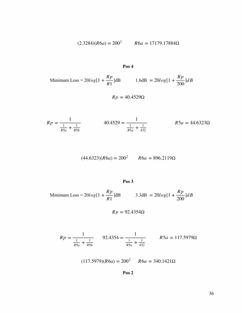
! ! Ω

Pos 4

Minimum Loss = 20 ! dB 1.6dB !

! Ω

! ! ! Ω

! ! Ω

Pos 3

Minimum Loss = 20 ! dB 3.3dB !

! Ω

! ! ! Ω

! ! Ω

Pos 2

(2.3284)(R6a) = 2002 R6a = 17179.17884

log[1 +RpR1

] = 20log[1 +Rp200

]dB

Rp = 40.4529

Rp =1

1R5a

+ 1R5b

40.4529 =1

1R5a

+ 1432

R5a = 44.6323

(44.6323)(R6a) = 2002 R6a = 896.2119

log[1 +RpR1

] = 20log[1 +Rp200

]dB

Rp = 92.4354

Rp =1

1R5a

+ 1R5b

92.4354 =1

1R5a

+ 1432

R5a = 117.5979

(117.5979)(R6a) = 2002 R6a = 340.1421

!36

Minimum Loss = 20 ! dB 5.2dB !

! Ω

! ! ! Ω

! ! Ω

Pos 1

Minimum Loss = 20 ! dB 7.4dB !

! Ω

! ! ! Ω

! ! Ω

log[1 +RpR1

] = 20log[1 +Rp200

]dB

Rp = 163.9402

Rp =1

1R5a

+ 1R5b

163.9402 =1

1R5a

+ 1432

R5a = 264.2029

(264.2029)(R6a) = 2002 R6a = 151.3990

log[1 +RpR1

] = 20log[1 +Rp200

]dB

Rp = 268.8458

Rp =1

1R5a

+ 1R5b

268.8458 =1

1R5a

+ 1432

R5a = 711.8504

(711.8504)(R6a) = 2002 R6a = 56.1916

!37

!

Figure 21. Curves created using schematic from Figure 19 and values from Table 5.

Table 5. Design Elements for “Pop” Filter Low Boost.

dB boost Rp Fb R5a R5b R6a R6b L1 in

mHC2 in

uF

Pos 1 2.3dB 268.8458Ω

500Hz 711.8504Ω

432Ω 56.1916Ω

92Ω 77.4042 1.9351

Pos 2 4.5dB 163.9402Ω

500Hz 264.2029Ω

432Ω 151.3990Ω

92Ω 77.4042 1.9351

Pos 3 6.5dB 92.4354Ω

500Hz 117.5979Ω

432Ω 340.1421Ω

92Ω 77.4042 1.9351

Pos 4 8.3dB 40.4529Ω

500Hz 44.6323Ω

432Ω 896.2119Ω

92Ω 77.4042 1.9351

Pos 5 9.6dB 2.3159Ω

500Hz 2.3284Ω

432Ω 17179Ω

92Ω 77.4042 1.9351

!38

To create the next two pieces of the equalizer the following criteria remain the

same: line impedance of 200Ω and an insertion loss of 10dB. To create the additional up

to ~10dB of reduction past the insertion loss, I have chosen to use type series impedance

filters before the bridged “T” attenuator for simplicity.

!

Figure 22. Response curves of the Waves REDD.51 Plugin for “Pop” filter high cuts -2,

-4, -6, -8, & -10.

100 1k 10k-80

-70

-60

-50

Frequency (Hz)

Mag

nitu

de (d

B)

Frequency Response

!39

"

Figure 23. Schematic of a Bridged “T” Series Impedance Shelving filter capable of

creating the curves depicted in Figures 13 and 22.

Referring to Figure 13 and Table 3, the following terms are needed to calculate

component values:

! !

! .0138H = 13.8mH ! 1.5915mF

The component values can then be calculated by simply if plugging the values into the

equations based on Figure 13 and Table 3. L1 and C1 are calculated slightly differently

here based on the original charts from Miller and Kimball (1938).

2! mH = 33.5588mH

R1A R1B

R5B

R6B

Bridged"T"Series

ImpedanceLowShelf

Filter

L1

R3

K − 1

K=

3.1623 − 11.7783

= 1.2159K

K − 1=

1.77833.1623 − 1

= .8224

L B =200

2π × 2300= CB =

1,000,0002π × 500 × 200

=

L1 = 13.8 × 1.2159 = 2(16.7794)

!40

! .6544uF

K values calculated from Figure 22 where the curves cross 10Khz.

Pos 5

R3= 2[R1(K-1)]

R3 = 2[200(3.2734-1)]

R3 = 909.36Ω

Pos 4

R3= 2[R1(K-1)]

R3 = 2[200(2.7542-1)]

R3 = 701.68Ω

Pos 3

R3= 2[R1(K-1)]

R3 = 2[200(2.2387-1)]

R3 = 495.48

Pos 2

R3= 2[R1(K-1)]

R3 = 2[200(1.7783-1)]

R3 = 311.32Ω

Pos 1

R3= 2[R1(K-1)]

R3 = 2[200(1.3964-1)]

C12

= 1.5915 × .8224 =1.3088

2=

!41

R3 = 158.56Ω

!

Figure 24. Curves created using schematic from Figure 23 and values from Table 6.

Table 6. Design Elements for “Pop" Filter High Cut.

dB Cut R3 Fb R5 R6 L1 in mH

Pos 1 2.9dB 158.56Ω 2300Hz 432Ω 92Ω 33.5588

Pos 2 5dB 311.32Ω 2300Hz 432Ω 92Ω 33.5588

Pos 3 6.9dB 495.48Ω 2300Hz 432Ω 92Ω 33.5588

Pos 4 7.8dB 701.68Ω 2300Hz 432Ω 92Ω 33.5588

Pos 5 9.6dB 909.36Ω 2300Hz 432Ω 92Ω 33.5588

!42

!

Figure 25. Response curves of the Waves REDD.51 Plugin for “Pop” filter low cuts -2,

-4, -6, -8, & -10.

!

Figure 26. Schematic of a Bridged “T” Series Impedance Shelving filter capable of

creating the curves depicted in Figures 15 and 25.

Next is the low cut section of the “pop” filter. K values calculated from Figure 25 where

the curves cross 40Hz.

100 1k 10k-80

-70

-60

-50

Frequency (Hz)

Mag

nitu

de (d

B)

Frequency Response

R1A R1B

R5B

R6B

Bridged"T"Series

ImpedanceLowShelf

Filter

R3

C1

!43

Pos 5

R4 = 2[R1(K-1)]

R4 = 2[200(3.02-1)]

R4 = 800Ω

Pos 4

R4 = 2[R1(K-1)]

R4 = 2[200(2.4547-1)]

R4 = 581.88Ω

Pos 3

R4 = 2[R1(K-1)]

R4 = 2[200(1.9498-1)]

R4 = 379.92Ω

Pos 2

R4 = 2[R1(K-1)]

R4 = 2[200(1.5488-1)]

R4 = 219.52Ω

Pos 1

R4 = 2[R1(K-1)]

R4 = 2[200(1.2162-1)]

R4 = 86.48Ω

!44

!

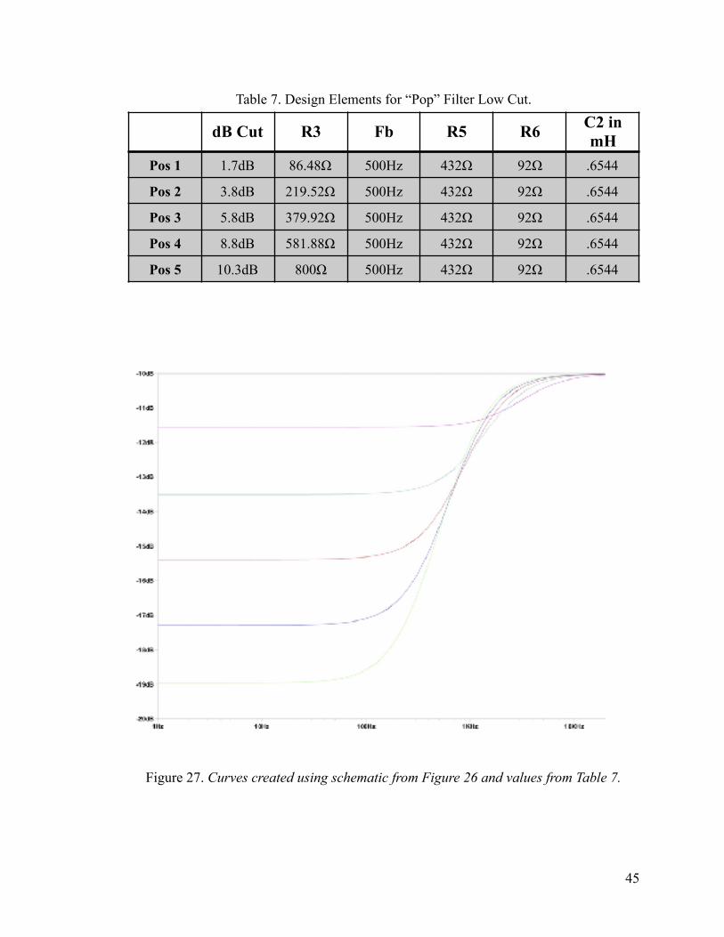
Figure 27. Curves created using schematic from Figure 26 and values from Table 7.

Table 7. Design Elements for “Pop” Filter Low Cut.

dB Cut R3 Fb R5 R6 C2 in mH

Pos 1 1.7dB 86.48Ω 500Hz 432Ω 92Ω .6544

Pos 2 3.8dB 219.52Ω 500Hz 432Ω 92Ω .6544

Pos 3 5.8dB 379.92Ω 500Hz 432Ω 92Ω .6544

Pos 4 8.8dB 581.88Ω 500Hz 432Ω 92Ω .6544

Pos 5 10.3dB 800Ω 500Hz 432Ω 92Ω .6544

!45

These four elements are then combined together to create a replica of the REDD

“Pop” Tone controls (Fig. 28).

! Figure 28. Schematic of REDD Tone controls for the “Pop” Plugin Module. Component

values listed do not represent practical real world components.

I determined the individual resistor values which are again calculated described

previously, by subtracting down the chain.

The Stereophonic System

The last part of the signal chain was E.M.I’s stereophonic system, which is

beyond my knowledge and skills to attempt to recreate; however, I documented the

R1A

200

R1B

200

R5B

432

R6B

92

.47µF

C1

3.36mH

L1

9.63Ω38.42Ω80.79Ω

R8

170.24Ω

R9R10

541.25Ω

L2

77.4mH

LowBoost

C3

1.3µF

R21

47.6Ω

R22

556.1Ω

R23

188.74Ω

R20

16282.79Ω

R24

95.21Ω

R25

56.19Ω

C4

.65µFR5

160.4Ω

R26

201.96Ω

R27

218.12Ω

R28

133.04Ω

R29

86.48Ω

0dB

R16

86.14Ω

R17

176.7Ω

R18

522Ω

R19

3321Ω

.085µF

C2

L3

18.85mH

+2dB +4dB +6dB +8dB +10dB

+10dB +8dB +4dB+6dB +2dB HighBoost

HighBoost+2dB +4dB +6dB +8dB +10dB

R12

2.33Ω

R13

42.3Ω

R14

72.96Ω

R15

146.61Ω

R30

447.65Ω

LowBoost

+2dB +4dB +6dB +8dB +10dB

-2dBLowCut

R31

184.16Ω

R32

152.76Ω

R33

158.56Ω

R34

206.2Ω

R35

207.68ΩHighCut

-2dB

L433.5588mH

-10dB

-10dB

REDDToneControlsSchematic-10dBinsertionloss

Constantimpedance-200ohm+-10dBLow&High

!46

individual sections of this system in the diagram for signal flow of the record path of the

desks (Fig. 29).

! Figure 29. Signal diagram of REDD desk record path.

Designing a Suitable Power Supply for the REDD.47 Preamps

I could not find much information on the power supplies for the REDD.47

preamps, other than a designation of REDD.43/D23/2. This unit was suitable for

powering preamps with the alternate circuit as shown in the schematic above (Fig. 29).

Because I could not find any usable information, I chose to design a tube power supply

capable of powering four REDD.47 units concurrently. The REDD.47 schematic tells us

then that this supply must be capable of supplying 120mA at 380V and 2A at 6.3V. With

this information, I could design a suitable supply. I have included my design and a few

!47

necessary calculations below, but have decided not explain this part in full because it is

not fully based on design information gathered about the REDD.51 Desk power supply.

!

Figure 30. REDD.47 Power Supply Capable of powering four REDD.47 units.

T1

120v

450v

450vV1 6CA4

BleederResistor

ToHeaters

L110H

REDD.4730mA

REDD.4730mA

REDD.4730mA

REDD.4730mA

380V FUSE

6.3v

REDD.47PowerSupply4x

CalculationsVL(VoltageLoad)=380vdcIL(CurrentLoad)=120mAVpeak-PI=VL+√2(VL)=917.32vIpeak=Ipavg(4)=240mA6CA4Uainvp=1,300vIp=500mAukf=500vLmin=1Hutreff=2x450vIdc=150mAL=10HUd.c.=378v

!48

Product: Sound Recordings

The major goal for my project was to replicate various techniques and effects used

at Abbey Road by The Beatles; consequently, the success of this goal could best be

determined by a practical implementation of my research. I produced three sound

recordings, each on two-inch analog tape. I used four tracks for one of the recordings,

which represented the number of tracks usually available to The Beatles while they were

recording at Abbey Road. I used eight tracks for the other two recordings. The Beatles

had an option to use eight tracks during recording sessions for their album entitled Abbey

Road, and for some of their recording sessions for their album that became known as The

White Album (Kehew & Ryan, 2007). I used four tracks to record the song “How The

Tune Goes” during an eight hour session (Table 8). I chose to record in a short session to

mimic the time constraint often imposed on The Beatles during their early years (1962–

1965), and also because of studio availability. In contrast, I used eight tracks during two

other sessions: an initial twelve-hour session and a subsequent eight-hour session. For

the eight track recordings, I used several effects heralded by The Beatles during their later

years (1966–1970). I relied heavily on Kehew and Ryan (2007) Recording The Beatles to

determine microphone choice and placement, effects used, and instrument placement

during the recording sessions. The following sections detail how I implemented the

above information during my recording sessions.

Effects

Because of innovative techniques that led to significant modification and

advancements of popular music during the 1960s, The Beatles and engineers at EMI are

!49

considered pioneers in popular music (Hecl, 2006). These innovative techniques include

implementation of effects, which were not necessarily invented at EMI, but were used on

popular sound recordings. A few examples, given in chronological order, include

backwards vocal or retrograde and varispeed on the song “Rain”, tape loops on

“Tomorrow Never Knows”, STEED on “Paperback Writer", and ADT on the Revolver

album (Kehew & Ryan, 2007, p. 265–311). What follows is an overview of the effects I

successfully implemented during my recording sessions.

Plate Reverb—This effect was only occasionally used while The Beatles were

recording at EMI. More often, an echo chamber was commonly used for spatial effects

on Beatles’ records. Nevertheless, I used plate reverb on my recordings because of the

availability of a plate and lack of availability of an echo chamber. EMI had four plates

available during the Beatle’s tenure, two with valve amplifiers and two with solid state

amplifiers (Kehew & Ryan, 2007, p. 282). The Beatles did use plates on recording

sessions for their album, Sgt. Pepper’s Lonely Hearts Club Band (Sgt. Pepper), and they

continued to use them during sessions for subsequent albums (Kehew & Ryan, 2007, p.

282).

Tape Echo/Repeat Echo—Although The Beatles were not the only artists to use

slap back echo, as they were with ADT, it was a commonly used effect that is simple to

recreate. Unfortunately, I was not able to incorporate either STEED or ADT in my

recordings. I successfully implemented ADT into songs recorded at the studios at MTSU

previously, but I could not at this time because one of the Studer tape machines in Studio

B was inoperable. Echo Chambers with pre delay were common practices at many

!50

studios during the 1960s, and involved sending a signal to a tape machine and taking the

delay created and sending that to an echo chamber to create a pre-delay. This was

specifically referred to as STEED at EMI studios when additional repeat echoes were

added. ADT is an effect that was invented by an EMI engineer, Ken Townsend, and

involves taking a vocal take and recording it to a separate tape machine, then varying the

speed of the second tape machine up and down to create a pseudo double track as the

vocal would vary in front of and behind the original (Kehew & Ryan, 2007). Tape echo

is created by sending the sound to be delayed to the record head of a tape machine, then

mixing the signal from the play head back with the original sound. Multiple delays can

be created by creating a feedback loop between the play and the record head. This was

referred to as repeat echo by EMI engineers (Kehew & Ryan, 2007, p. 285).

Half-Speed Overdubbing.—Perhaps the most notable example of use of half speed

overdubbing by The Beatles is the piano solo by George Martin on the song “In My

Life.” The overdubbing effect is created by recording a part at half the intended playback

tape speed and an octave lower than intended to be heard (Kehew & Ryan, 2007, p. 289).

The part recorded will be an octave higher than when recorded when played at the

intended speed.

Frequency Control (Varispeed).—Varispeed is similar to half speed overdubbing,

but instead of running the tape at half the playback speed, the speed is variably adjustable

up and down. The first Beatles first used this effect on the song “Rain.” The backing

track was recorded at a faster speed than final playback, and the vocals were recorded at a

slower speed than the final play back (Kehew & Ryan, 2007, p. 293). The Beatles

!51

apparently appreciated the sound created by varispeed as this was one of their most often

used effects, which was used on dozens of their songs.

My Recordings.—All recording sessions for my album took place in Studio A and

B in the John Bragg Building at MTSU. Studio A is the largest open-space recording

studio; consequently, I used Studio A to approximate Studio Two at Abbey Road, which

consisted of a single open recording space. Studio B is a smaller recording studio that is

subdivided into several small, separate recording spaces; consequently, I used it as a

substitute for Studio Three at Abbey Road, which consisted of small, subdivided rooms.

I used eight different types of microphones. I used five microphones from the MTSU

collection, including a Coles 4038 and an AKG d20. I chose these microphones because

they are good approximations of two microphones used by The Beatles, the STC ribbon

and AKG D12, respectively. I built three microphones, which were replicas of the

Neumann U67, Neumann U47, and the AKG C12.

Before I began to work in the studio, a friend (Dylan Miller, no relation) and I

wrote several songs, and we recorded acoustic and vocal demos of each of these songs. I

recruited members from The Busks (Dylan Miller, Wesley Sadler, and me) as musicians

for the recordings. Wesley played drums on “Neon Sunrise”; whereas, Dylan and I

provided vocals, drums, and played several instruments on all recordings. I did not make

a decision on which songs to record until we were in the studio and ready to record.

Also, I chose microphones during the pre-production stage, primarily based on what was

available at MTSU and in my own collection.

!52

Although I decided on which microphones to use during pre-production, I chose

all outboard gear, and pre-amps when we started to record. Unfortunately, I was not able

to construct any REDD.47 preamps as originally planned. The use of gear, instruments,

microphone placement, and effect implementation is covered in a synopsis of the

recording process for each sound recording below.

How The Tune Goes

Recording Synopsis—“How The Tune Goes” was the last song I recorded and consisted

of an eight hour tracking session, with about two hours allocated for mixing on a different

session. The session began at 12am. At this time, I discussed song options with my

recording partner and decided on this particular song while we setup to track the drums

and an acoustic twelve string guitar in an isolation booth. I was acting as musician and as

a recording engineer during this session as well as all others; consequently, it took me

Table 8. “How The Tune Goes” Tracks

Take I Track I Track II Track III Track IV

Drums, 12 String Acoustic

Vocal Vocal

Tracks III & IV bounced to I

Vocals Drums, 12 String Acoustic

Electric Guitar, Piano

Bass, Tambourine

!53

longer than anticipated to set appropriate levels between the two instruments. When the

levels were finally set to my satisfaction, I decided to keep the first take, or first attempt

at recording the song. I then overdubbed two vocal tracks, each in a single take. One

vocal track was recorded in the isolation booth and one in the open room. These tracks

were originally intended to serve as guide vocals for overdubs, but I kept them in the

interest of time and track availability. I then bounced the two vocal tracks to a single

track, to which I added piano and electric guitar with their own shared track. This took

about an hour as the two of us worked out our parts and a harmonized instrumental break.

At approximately 5am, I overdubbed a bass guitar with tambourine to the final open

track, and put together a rough mono mix. The three of us left the studio at

approximately 7am, with the entire song recorded, but not mixed. Although there were

imperfections in the ending and in the vocal tracks, I did not think that the imperfections

were serious enough to warrant scrapping the recording. My goal was to use four tracks

to create a mono record, which I had accomplished. For the final mix, I let the tracks dry,

in homage the relatively dry soundscape of the Revolver album. The recording was

influenced primarily by the albums Help! and Revolver.

Instrument & Amp Usage Synopsis.—I chose the instruments and amps used on

this recording to reflect as closely as possible the instruments used by The Beatles in their

1965–1966 era, which is when the albums Help!, Rubber Soul, and Revolver were

recorded. I used a 12 string acoustic guitar to pay tribute to John Lennon, who played a

12 string guitar on the song “Help!” (Kehew & Ryan, 2007). Furthermore, I used an

electric Epiphone casino with flat wounds, Hofner bass with flat wounds, and a replica

!54

VOX AC30 amplifier, which were similar makes and models as those used by the Beatles

(Kehew & Ryan, 2007). Also, I used the Kawai grand piano available in Studio A, a

Mapex drum kit, and a tambourine during tracking of this recording.

Microphone Usage Synopsis.—I used only four different microphones during this

recording, each of which was chosen to reflect common microphone practices used by

The Beatles during their recording sessions. As an overhead for the drums, I placed a

Coles ribbon microphone directly above the snare, near head-level of the drummer. I

rounded out the drum kit microphones with an AKG d20 on kick and a Neumann KM84

underneath the snare, and I flipped the polarity of this signal. I modeled this entire setup

after the 1966 microphone setup for drums by Geoff Emerick, as shown in Recording the

Beatles (Kehew & Ryan, 2007, p. 411). I also used the Coles 4038 microphone for the

piano. I used a replica U47 on the acoustic and electric guitars, and on the vocals. I used

close miking techniques for most microphone placements. The drum overhead was a few

feet from the top of the snare, all other microphones were within a foot of the sound

source intended to be captured.

Effects Usage Synopsis.—I recorded the base track for this song a half step down

and sped up to E at 15ips. Instead of implementing a multitude of effects, I used this

recording to focus on the use of internal bouncing to free up track space. This is a simple

example of track reduction, with just the use of one generation. As illustrated in Table 8,

the vocal tracks were recorded to tracks III and IV and then internally bounced to track I

to free up space for additional overdubs.

!55

Outboard Gear Usage Synopsis—The only outboard gear used in Studio A was a

VariMu Compressor, an 1176 compressor, and the API equalizer modules. The

compressors were used between the input of the tape machine and the output of the

console as this is where a compressor was always in the chain recording The Beatles

(Kehew & Ryan, 2007).

Neon Sunrise

Recording Synopsis—I initially intended to use Neon Sunrise only as a practice

session and demo for thesis material, but I eventually chose to include this song because

it illustrates several techniques used by The Beatles and follows a similar technical

restriction process. Instead of using four tracks, I used eight tracks (Table 9), which were

available to The Beatles during their later White Album sessions and for the entirety of the

Abbey Road sessions (Kehew & Ryan, 2007, p. 511). I used Studio B for all tracking

sessions. I tracked together live recordings of drums, an electric guitar, and an acoustic

guitar to one track and in one take; however, several takes of rehearsals were recorded as

I set levels. This was a fairly quick process, which was completed in less than two hours

Table 9. Neon Sunrise Tracks

Take 3 Track I Track II Track III Track IV Track V Track VI Track VII

Track VIII

Drums, Electric Guitar, Acoustic Guitar

Electric Guitar

Piano BKD Vocal

Vocal Vocal Bass

!56

from load in. I then developed an electric guitar part that mimicked the rhythm guitar

part on track one. It was recorded through an AC30 amplifier with tremolo on the next

track, followed by a piano part inspired by the cartoon Rugrats’ theme song on track III.

I then recorded two vocals to tracks IV and V, background harmonies to track VI, and

finally, bass was recorded, direct injection, to track VII. I then bounced a quick stereo

mix for this song. Unfortunately, this would be the only bounce before the vocals were

accidentally erased. The whole process took approximately five hours.

Instrument and Amp Usage Synopsis.—The Epiphone Casino was again used for

all electric guitar parts and the Hofner for bass parts. The electric guitars were run

through a replica VOX AC30. A custom Dark Horse drum kit was used for drums, and a

miniature martin acoustic for acoustic guitar. I also used the Kurzweil piano in studio B.

Microphone Usage Synopsis.—The microphone choices made on this recording

are similar to those used on “How the Tune Goes.” The microphone choices for drums

were an expansion of the three described earlier, and were inspired by a later microphone

setup for drums used by Geoff Emerick during 1967 as pictured in Recording The Beatles

(Kehew & Ryan, 2007, p. 436). I added two Yamaha MZ-204 microphones to the toms

and a Sennhieser MD421 to the hi-hat. I used a replica U67 microphone for both electric

guitars and for all vocals. I recorded the acoustic guitar with a replica U47, and the piano

with a replica C12. The bass was run direct injection. Close miking techniques were

similarly employed as on “How The Tune Goes”.

Effect Usage Synopsis.—This recording features extensive use of the varispeed

recording technique and of half-speed overdubbing. I recorded the base track containing

!57

drums, acoustic guitar, and electric guitar, a half step down in Bb at 14.16ips and played

back at 15ips in B. The piano track was recorded as two different sections. One section

was recorded at half speed, the other at normal speed. The first verse was the portion

recorded at half-speed, and tape echo and echo repeat were applied throughout both

sections. I also recorded the overdubbed guitar a half step down, similar to the base

track. I recorded both vocal tracks with varispeed applied; one track slightly above 15ips

and the other slightly below 15ips, and both within a semitone. I double tracked the

harmony vocals, which were both recorded slower than 15ips, with one a whole step

slower, and the other a few more steps slower than this. These speeds were randomly

chosen. When played back at full speed, it created a fast vibrato effect due to the sped-up

natural vibrato of the voices. I used the tape echo and repeat echo effects frequently on

this recording. For example, the overdubbed guitar, the double tracked vocal, and the

piano all feature this effect.

Words

Recording Synopsis.—“Words” was the second song I recorded for this project,

and the second I recorded in studio B. This song was tracked and completed during two

separate sessions. The original tracking session was performed as a tag-on at the end of

the “Neon Sunrise” session. This track was notably influenced by several songs by The

Beatles, including “A Day in the Life”, “Hello, Goodbye”, and “Lucy in the Sky with

Diamonds.” The base track consists of piano and guitar on the same track I, with a live

vocal performance recorded simultaneously to track II (Table 10). This vocal was

subsequently overwritten with another vocal during the following overdub session.

!58

During the next session, two vocals takes were completed and recorded to tracks two and

three, overwriting the original vocal take. A Hammond B3 was recorded onto track VI,

an electric guitar on track VII, followed by drums on track VIII. A bass was the final

overdub completed on track IV. Background harmony vocals were originally planned for

track V, but this never came to fruition. I used several different effects on this song,

including as Leslie’d electric guitar, plate reverb, varispeed, tape echo/repeat.

Furthermore, this is also the only recording for the project to use a bass amp instead of

direct injection to record the bass.

Microphone Usage Synopsis.—This recording uses the same mic setup for drums

as “Neon Sunrise”, again modeled after the drum setup of Geoff Emmerick during 1967.

I used a replica AKG C12 microphone to capture the piano. I used a different

microphone to capture the vocals on this recording compared to the other recordings. I

used a Coles 4038 ribbon to combat a particularly strident voice and to give the recording

an overall darker tone. I took great care to prevent plosives of air from damaging the

ribbon element. For example, I included a pop filter and positioned the microphone at an

angle tilted away from the singer’s voice to prevent direct breathe from blowing on the

thin aluminum. I used the replica U47 microphone and Leslie cabinet for both the guitar

and organ. I attempted to mimic the setup of the bass to that used by Paul McCartney

during The Beatles’ later years (1967-1969). I was a bit disappointed by my results,

which I thought inferior to that of McCartney. I attributed my poorer recording to the

absence of a few key elements, including Paul McCartney, a Rickenbacker bass, and the

RS127 compressor. The bass was recorded on a Hofner into a Fender Blonde Bassman

!59

located in the center of Studio B, and was mic’d by a replica AKG C12 approximately

twelve feet away.

Effect Usage Synopsis.—“Words” was an effect laden recording. I used several

Beatles’ effects in an attempt to create a particular sound. These effects included

extensive plate reverb, repeat echo, and varispeed.

Post Production

Although I completed the stereo mix for “Neon Sunrise” at the end of the initial tracking

session, I did not complete the mono mix at this time. Unfortunately, I inadvertently

erased the two vocal tracks; therefore, the mono mix is noticeable different from the

stereo mix (it lacks melody vocal). Differing mono and stereo mixes is actually a

common occurrence among mixes of songs of The Beatles; however, there are none that

completely lack a vocal. For example, the mono and stereo mixes of “Lucy in the Sky

with Diamonds” from the (Sgt. Pepper) album are very different from each other with the

mono mix having much more phasing applied to the vocal (Kehew & Ryan, 2007). I

completed all of my other mixes on separate session from their tracking session.

Table 10. “Words” Tracks

Take 3 Track I Track II Track III Track IV

Track V Track VI

Track VII

Track VIII

Drums, Piano

Vocal Vocal Bass Hammond B3

Leslie Guitar

Drums

!60

Because of difficulties associated with studio availability, time constraints, and

cost, I printed my masters to a digital format. Having a digital master, rather than a

master tape, facilitates presentation (I do not need to transport a 1/2in tape machine for

presentation) and reduces cost on the purchase of magnetic tape.

“How The Tune Goes” Mono Mix.—I applied additional compression and

equalization to the mono mix for this song, but not for the other recordings. This is

perhaps because unlike the others, I completed the mono mix before the stereo mix, and I

was concerned about losing elements because of masking primarily associated with

dryness of the track as there was no space between elements. Furthermore, this song was

more hastily recorded and needed additional brightening and taming of the vocal. I had

to dynamically adjust the bounced vocal with the fader throughout the print, primarily

between sections, and the intro/exit, because of noise floor created by improper levels

when recording.

“How The Tune Goes” Stereo Mix.—With the stereo mix for this song, I chose to

leave the non-vocal tracks as they were and only use panning to ensure clarity in the

stereo spread. I followed a fairly conventional early Beatles’ stereo mix of panning both

vocals collapsed towards center, but with enough spread to balance the stereo field, the

drums and bass slightly to the left (as these were usually on the track in the 1962-1965

days), and the overdubbed guitar/piano track hard right (Kehew & Ryan, 2007). The

vocals received additional equalization and compression. The ending for the stereo mix

differs from that of the mono mix. In the mono mix, the song fades out on an acoustic

!61

guitar strum; whereas, in the stereo mix, the song fades out the electric guitar and piano

sounding.

“Neon Sunrise” Mono Mix.—I gave very little thought or time to this mix

because there were no vocals, and not enough time available to redo them. With this

mind, I worried very little about elements competing with one other and fairly quickly set

suitable levels and printed the mix. Mono mix notably does not fade out like the stereo

mix.

"Neon Sunrise” Stereo mix.—The stereo mix for this song was intended to be

kept within the options available to The Beatles during their later years (Abbey Road

sessions) on the TGI desk. It was completed immediately following the tracking session.

Only levels and panning were adjusted, as no additional time based effects, equalization,

or compression were needed. Many of these effects had already been printed to the

recorded tracks, such as the repeat echo on the vocal. This is similar to how the slapjack

on John Lennon’s voice on “A Day in the Life” was recorded to tape concurrent with his

vocal take and was piped to his headphones (Kehew & Ryan, 2007).

“Words” Mono Mix—This mix notably differs from the stereo mix because of the

exclusion of the drums until the second verse. The vocals are more present in the mono

mix as well as the Leslie guitar.

“Words” Stereo Mix.—The stereo mix is very simple with no additional effects added.

The piano/acoustic track panned slightly left of center and the drums fairly hard right.

The vocals are split one down the center the other slightly to the right, this was

commonly how The Beatles’ engineers would pan vocals when applying ADT to stereo

!62

mixes, although the ADT signal was often hard panned (Kehew & Ryan, 2007). The

bass, organ, and Leslie guitar are kept near the center.

I believe that ultimately each artist sound comes from the artist itself, and I think

this project further enhances this notion. While albums recorded in a completely digital

format sound may sound completely different from my results, this likely has more to do

with the artist than the format, and even more to do with intent. I chose to record these

songs in an analog format influenced by The Beatles. I hope ultimately listeners can tell

this with playback. Although I may not have been able to complete all that I set out to

do, I know that I have laid a solid foundation for me in this thesis to continue my research

for many more years.

!63

References

Brice, R. (2013). Music electronics. Hampshire: Transform Media.

Cox, R. A., Felton, J. M., & Chung, K. H. (1995). The concentration of commercial

success in popular music: An analysis of the distribution of gold records. Journal

of Cultural Economics, 19(4), 333-340. doi:10.1007/bf01073995

Hecl, R. (2006). The Beatles and Their Influence on Culture (Unpublished bachelor's the-

sis). Masaryk University. Retrieved from https://is.muni.cz/th/108918/ff_b/

The_Beatles_and_Their_Influence_on_Culture.pdf

Kehew, B., & Ryan, K. (2007). Recording the Beatles: The studio equipment and tech-

niques used to create their classic albums. S.l.: Curvebender Publishing.

Miller, W. C., & Kimball, H. R. (1938). Motion Picture Sound Engineering: A series of

lectures presented to the classes enrolled in the courses in sound engineering giv-

en by the Research Council of the Academy of Motion Picture Arts and Sciences,

Hollywood. New York: Van Nostrand.

Miller, W. C., & Kimball, H. R. (1944). A Rerecording Console, Associated Circuits, and

Constant B Equalizers. Journal of the Society of Motion Picture Engineers, 43(3),

187-205. doi:10.5594/j08003.

REDD, (1959) The EMI Stereosonic Recording Circuits: Sum & Difference, Spreader

and Shuffler. EMI REDD department REF. RSL.51

Tremaine, H. M. (1959). Audio cyclopedia (1st ed.). Indianopolis, Ind.: Sams.

WAVES, (n.d.) Waves REDD.37-51 User Guide.

!64