An image construction method for visualizing managerial...

Ž .Decision Support Systems 23 1998 371–387

An image construction method for visualizing managerial data

Ping Zhang )

School of Information Studies, Syracuse UniÕersity, Syracuse, NY 13244, USA

Abstract

High volume data with complicated relationships can render human decision-making a frustrating task. Computer-gener-ated visualization is an approach that can assist decision-makers in gaining insight into the data so that eventually superiorsolutions can be developed. Current research in visualization has addressed how to deal with high volume data that have

Ž .some inherent structures such as hierarchy, network, or geographical relationships . Many management domains, however,have data that lack obvious structures to provide a base for computer-generated visualization. This paper reports a speciallydesigned technique for visualizing such management data. Data objects involved in the decision-making tasks are assigned

Ž .with geometry called visual abstract in Euclidean space. Then a set of image construction rules are applied to connectmultiple visual abstracts into images that can be displayed on a computer screen. We use two business domains,manufacturing production planning and resource constrained project scheduling, to illustrate this visualization technique.q 1998 Elsevier Science B.V. All rights reserved.

Keywords: Information visualization; Decision making support; Manufacturing production planning; Project scheduling with resourceconstraints and cash flow

1. Introduction

Human decision making is a vital but frustratingtask in many management domains. High volumes ofcomplicated data, complex relationships among thedata, negotiability of constraints, changing environ-ment, and time pressure are typical challenges thatdecision-makers must face. Human information pro-

w xcessing capacity 3,34,42 limits our ability to di-rectly handle situations that are too complicated and

) Tel.: q1-315-443-5617; fax: q1-315-443-5806; e-mail:[email protected]

involve a high volume of data. Most existing Deci-Ž .sion Support Systems DSSs are either large-scale

systems built to facilitate well-defined and repetitivedecision tasks, or else they are small PC-based sys-tems offering quick and economic routines to sup-

w xport one-time decision making 22 . These DSSsprovide algorithm-based solutions that have built-infunctionality with limited flexibility to reflect chang-ing environments and possibilities for negotiation.Thus they often fail to provide complete solutionsfor complicated managerial decision problems.

Computer-generated visualization offers an alter-native approach. Long before computers were used,people had already noticed the importance of com-municating information, especially complicated in-

wformation, using graphical representations 7,9,46,

0167-9236r98r$ - see front matter q 1998 Elsevier Science B.V. All rights reserved.Ž .PII: S0167-9236 98 00050-5

( )P. ZhangrDecision Support Systems 23 1998 371–387372

x47,50 . For example, statisticians use graphs to un-derstand complicated relationships between multiplevariables and to discover important information hid-

w xden in the data 12,45 . Representations play animportant role in solving problems in the field ofArtificial Intelligent, where visual representations areseen as data structures for expressing knowledgew x31,41 . Appropriate representations can facilitateproblem-solving and discovery by providing an effi-cient structure for expressing highly abstract data.This is because cognitive efficiency results whenperceptual inferences replace arduous cognitive com-

w xparisons and computations 32 . Therefore, effectivevisualization can shift some of the user’s cognitiveload to the human visual-perception system: lettingpeople see—perceptually—what they need to ‘see’—cognitively—so that they do not have to puzzle

w xthings out on a strictly cognitive basis 52 .Scientific visualization is a field that has enabled

the visualization of large volumes of scientific dataw x16,33,38,40 that are either gathered from the worldand then analyzed by a computer, or produced

w xthrough computer simulations 56 . Large volumedata means a large number of data objects that have

Ž .extensive data elements entity instances in eachdata object. Typical uses of scientific visualizationtechnology involve the visualization of data that arerepresented as two- or three-dimensional objects.Computer-generated representations of these datamimic the real-world objects or scenes these data areabout. Abstractions may apply in the representations,as long as human eyes can detect the same patternsas those that exist in the corresponding real-worldobjects or scenes, and when other details are notnecessary for the point of interest. Examples can befound in many applications, such as visualizing bio-logical molecules, medical imaging, or tracking andimaging elementary particles.

Recently, efforts have been made to visualizelarge volume data that do not necessarily have inher-ent geometry in the data objects to lead tocomputer-generated representations. This type of vi-sualization is known as information visualizationw x24 . Special challenges for information visualizationinclude creating concrete visual representations thatutilize human visual perceptual capability and en-hance human information comprehension. For exam-

w xple, TreeMaps 2,43 is designed to visualize huge

amounts of hierarchical and categorical informationsuch as file directories, budgets, sales data, andorganizational structure data. More than a thousanddata elements can be visualized in TreeMaps. Asecond example is the work at AT&T that hasfocused on visualizing network-related and geo-

w xgraphically related data 4,20 . Other examples in-clude SemNet for visualizing knowledge base infor-

w xmation using a hierarchical context 21 , and ConeTrees for visualizing huge information hierarchiesw x10,39 . Yet another example is the Geographic In-

Ž .formation Systems GIS type of visualization sys-tems, which uses the geographical structures amongdata objects. In summary, these information visual-ization studies, and the visualization systems thatemerged from them, address the high volume of datathat is typical in managerial decision-making do-mains.

Data representations and their impact ondecision-making performance have been a subject of

wInformation Systems research for some time 6,17–x19,26,48 . The graphical representations in most

studies in this area are primarily limited to popularstatistical charts, such as pie, line, and bar, amongothers. The limitations of statistical graphs, however,are twofold. First, most data variables to be graphedmust have a limited number of data elements. Sec-ond, the number of data variables in a graph islimited. There are some techniques for dealing withmultiple data variables. Yet for most of such tech-niques, a trade-off between number of variables and

Ž .the cardinal number the number of data elements ofw xeach variable has to be considered 11,12 . Neverthe-

less, the commonly used statistical graphs or chartsare not necessarily designed to support any specificdecision tasks or processes. Thus the focus of Infor-mation Systems studies has been limited to simpledecision tasks with small data volume and simpledata relationships.

Other research results in management data visual-w xization include those by Jones 28,29 and visual

Ž . w xinteractive simulation VIS for modeling 5,25 .Jones used attributed graphs and graph-grammars forrepresenting management science models such asdecision trees, linear programming, and critical pathsthat involve network-related relationships. Here thedata volumes are not high and the relationshipsamong the data objects are hierarchy or network

( )P. ZhangrDecision Support Systems 23 1998 371–387 373

based. Visual interactive simulation for modeling‘uses a simulation model where the user can suspendexecution of the model, modify one or more parame-ters, including the model structure, and resume model

w xexecution’ 5 . VIS focuses on visual representationsŽand animation of a simulation model can be ab-

.stract and on illustration of the execution of themodel. VIS techniques capture the dynamic aspectsof a simulation model with a limited number of dataobjects.

However, most management domains have multi-ple data objects that do not have a hierarchy ornetwork based relationship among them. The rela-tionships among the data objects can be very compli-cated with no obvious structure at all. The challengefor creating a visual form for the data is thus two-fold:to create a visual form for each of the data objectsinvolved, and to create a visual form to represent therelationships among the data objects. To date, thistype of information visualization is nearly non-ex-istent. Current visualization tools, such as IBM DataExplorer, AVS, and IRIS Explorer, are designed forscientific visualization purposes and are very diffi-cult to use for visualizing managerial data. Specialvisualization techniques have to be developed toaddress the special nature of the managerial data.

Visualization can mean different things and tech-Žniques to different researchers in different fields see

a summary of visualization research for Operationsw x.Research in Ref. 30 . In this study, we define

information visualization as a process for transform-ing data into visual forms in order to allow users tocomprehend and interact with information more ef-fectively.

This paper reports part of the current results ofour long-term research effort to discover laws foreffective human-information interaction and to de-velop management information visualization tech-niques for supporting managers solving decision

w xproblems 53 . In the current research, we explorethe feasibility of developing visualization systems tosupport decision-makers in making difficult deci-sions in a dynamic environment. We focus on thetechnique of building information visualizations ofseemingly non-visual data that are massive in bothvolume and dimension; these visualizations help de-cision-makers to achieve data comprehension andeventually improve their problem-solving perfor-

mance. This paper reports a visualization techniquewe have developed. We test the technique by apply-ing it to two management domains: manufacturingproduction planning, and project scheduling withresource constraints and cash flows.

The remainder of the paper is organized as fol-lows. Section 2 describes the characteristics of man-agement domains and their data that our research hasfocused on, with two business domains as examples.Section 3 introduces the image construction tech-nique. In Section 4, we apply the visualization tech-nique to the two business domains. Section 5 drawsconclusions from the current research and points outfuture directions.

2. Management data for decision-making

Our research focuses on management domainsthat have the following characteristics:1. There are high-volume data that domain users

have to deal with in order to solve decisionproblems.

2. The relationships among the data are complicatedand often have no obvious structure.

3. Computers are vital in managing and providinginformation; however, the final decisions or solu-tions are made or developed by human beings.

4. The decision-making environment is dynamic,which requires decision-makers to understand asmuch as possible about problem situations and thepotential for solutions.

5. Time pressure requires decision-makers to re-spond quickly to impending events.In this section, we briefly describe two manage-

ment domains that have the above characteristics:manufacturing production planning and projectscheduling with resource constraints and cash flow.In doing so, we point out the technical challenges ofvisualizing this type of data and provide a contextfor discussing the design of visual abstracts andimage construction rules, to be discussed in Section3. Later, in Section 4, we revisit these two domainsand examine the application of the technique tothem. Our ultimate goal is to develop effective visu-alization methods that can be used in more than onebusiness domain to develop high conceptual level


images that enhance decision-makers’ data compre-hension.

2.1. Manufacturing production planning

Ž .In a collaborative effort with IBM Austin, TX ,we studied the production-planning problem at IBM

Ž .PC Electronic Card Assembly and Test plant ECAT .This problem was ideal for this study because of thevast quantities and multiple dimensions of data andconstraints, the typical dynamic environment for de-cision making, the need for rapid data comprehen-sion under time pressure, and the heavy humaninteractions with information during decision-makingprocesses. In order to make our results applicable toother manufacturing production-planning domains,we compared planning process in ECAT to the stan-

w xdard MRP II process 13,49 and decided to use theMRP II process as a generic planning process with asimplified structure for the bills of material. In ourstudy, products use components; components use noother components.

In manufacturing production planning, a planner’sgoal is to maximize overall revenue from the produc-tion, subject to resource constraints such as tools andcomponent availability. A typical manufacturer canhave hundreds of different products and thousands ofdifferent components. Some of the components areused by several different products and thus are named‘common components.’ Different production assem-

Ž .bly lines also called Production Pull Lines, or PPLsshare tool capacity and components during produc-tion. A production plan can span several weeks. Thedecision-making environment is dynamic. For in-stance, there often is a severe component shortageproblem. Among all short components, however,only a very few components are ‘critical’ or bottle-neck components. During the planning period, plan-ners can take many possible actions in order to solvesome of the problems or sub-problems. For instance,they can change the quantity of products to be made

Ž .in each week this is called demand , can movedemand to different assembly lines to change pro-duction loads, or can move demand to different timeperiods within the same assembly line. They canadjust an assembly line’s capacity by adding orremoving tools. They can change the quantity of

Žcomponents to be received that is, scheduled re-

.ceipts , and change the distribution of componentsŽ .over products named production mix . In such a

dynamic environment, the planner’s understanding ofthe planning problem situation is crucial.

Owing to the complicated relationships amongdata and the dynamic decision-making environment,existing production planning systems, such as vari-

Žous MRP II systems some of them are available at.ECAT and some simulation systems, cannot provide

complete solutions for production plans that reflectthe changing constraints and environment. Some ofthese systems have friendly user interfaces and pro-

Žvide simple one- or two-dimensional graphs line.charts, bar charts, pie charts, etc. of certain data.

However, most data these systems can provide are intabular format: they are either limited to the size thata computer screen can handle, or printed as a reportthat may be several hundred pages long. Data dis-played in these ways do not give planners a clearvision of what is going on. In other words, theyshow ‘trees’ but not the ‘forest’ of the planningproblems. Before trying any possible actions, theplanners need to use their cognitive powers to figureout the ‘stories’ behind the data, such as identifyingthe global patterns of the shortage or the criticalcomponents from all shortfall components.

2.2. Project scheduling with resource constraintsand cash flow

Another domain used in the study is projectscheduling with resource constraints and cash flow.In general, a large project can be broken down intomany smaller activities. Each activity has an esti-mated duration, resource requirements, and possiblyassociated cash flows. The resource constrained pro-ject-scheduling problem with cash flows addressesthe scheduling of a number of activities subject toconstraints on precedence requirements and resourcelimitations. A series of cash flows occurs over theduration of the project in the form of cash outflowsfor project expenditures and cash inflows as pay-ments for completed activities.

Fig. 1 depicts an example project network. This isan activity-on-node representation. Each node repre-sents an activity and the directed arcs represent theprecedence relationships among activities. Each ac-

Ž .tivity i is1, . . . , m has a fixed duration d ,i


Fig. 1. Example project network.

Ž . Žresource requirements r , . . . , r of k types ini1 i k.this example ks3 , and cash flows F and Fo i

representing expenses and payments. The label asso-ciated with activity C, for example, has three com-

Ž .ponents: cash flows outflow 16, inflow 41 , re-Ž .source requirements 6,1,4 and duration 2. Analo-

gous labels are associated with other activities. Thefirst cash flow associated with an activity is non-positive, represents the cost of the activity, and isincurred at the activity’s start time; the second cashflow is non-negative, represents the payment forcompleting the activity, and is obtained at the activ-ity’s completion time. In this study, we assume thatresources are renewable. Duration, expense, and pay-ment associated with each activity are known. Theexpense occurs at the beginning of the activity, whilepayment is made at the completion of the activity.

Resource-Constrained Project Scheduling Prob-lems are widely encountered in practice, in situationsranging from architectural construction to softwareproject management and research and development.The problem is generally concerned with thescheduling of a project consisting of a number ofactivities that are linked together by precedence rela-tions and multiple resource restrictions. When cashflows exist in the form of expenses for initiatingactivities and payments for completed work, thedevelopment of project schedules that maximize the

Ž .net present value NPV of the project is of consider-w xable practical importance 8 . This is a difficult

combinatorial optimization problem that precludesw xthe development of optimal schedules 23 . In partic-

ular, as the size of a project increases, or as parame-ters such as duration and resource requirements ofthe project change, it is even harder to generate goodschedules in a reasonable time. Many heuristics havebeen proposed in the literature to solve the resource-constrained project scheduling problem with cash

w xflows 15,58 , with the primary focus on proposingefficient solution procedures in a predictive schedul-ing environment.

The current studies are mostly limited to thedeterministic nature of the problem. In reality, how-ever, those parameters such as activity duration,resources, and cash flows may change in response toexternal unexpected occurrences or constraints. Un-

Žder certain circumstances, resources including rawmaterials, machines, and human resources as well as

.capital budgeting originally promised may not bereadily available. These may influence the duration,the time to complete certain activities. The capitalbudgeting constraints may also have a direct impacton the cash flows. In the event that such uncertain-ties occur, the initial solution obtained from algo-rithms or heuristics may not be good or even feasi-ble. Project managers have to be able to react to such


uncertainties in a timely fashion by making properadjustments to the current schedule. The massivenessof data and relationships typically overwhelm man-agers. Given suggested solutions from differentheuristic algorithms, managers have to understandthe relationships among all the variables involved,such as precedence relationships, resource limita-tions, cash flow patterns, etc. Based on their under-standing of the scheduling situation, managers maytake some actions toward adjusting schedules inorder to achieve better results. Without an intelligenttool to assist in such a complex decision-makingprocess, project managers will easily be at a loss andeven fail in managing such risks. This is a criticalproblem, and it presents a good opportunity forinformation visualization techniques to play an im-portant role.

3. A method for management information visual-ization

Owing to the non-visual nature of the data to bevisualized, at this time information visualization canbe more art than science or engineering, as pointed

w xout by Tufte 47 : ‘‘the use of abstract, non-represen-tational pictures to show numbers is a surprisinglyrecent invention.’’ However, a set of principles ‘leadsto changes and improvements in design, suggestswhy some graphics might be better than others, and

w xgenerates new types of graphics’ 47 .In our approach to visualizing the non-visual, we

design ‘visual abstracts’ for each data object in-volved in the problem-solving and decision-makingprocesses. Then we link the visual abstracts as‘images,’ using a set of image construction rules wehave developed.

To be represented in a 2-D Euclidean space, eachof the data objects must have a basic geometric

Ž .structure called ‘visual abstract’ . The visual ab-stract of a data object should be used consistently asa building block of more complicated visual repre-sentations by the visualization system for a businessdomain. Some data objects may be easier to repre-sent with geometry than others may. For example,we can use a line segment as the visual abstract forthe concept of time. A line segment can also be usedfor locations, such as product assembly lines at

ECAT. For many other data objects, however, wehave to create a visual abstract based on severalrationales discussed below.

People are accustomed to using different graphi-cal representations in their jobs and in daily life.They have similar ways of interpreting visual images

w xand classifying them 32 . This should provide afoundation for designing specific visual representa-tions of certain types of information. While graphdesigners have the freedom to design different graphsfor the same data and readers can prefer one designto the other, the problem of constructing visual

w xrepresentations is efficiency 7 . Bertin applied thenotion of ‘mental cost’ to visual perception. Hestated that ‘‘if in order to obtain a correct andcomplete answer to a given question, all other thingsare equal, one construction requires a shorter obser-vation time than another construction, we say that it

Žw x .is more efficient for this question’’ 7 , p. 9 .Efficiency is linked to the degree of facility char-

Žw xacterizing each stage in the reading of a graphic 7 ,.p. 139 . To read a graphic is to proceed more or less

rapidly in three successive operations, asking: Whatdata objects are involved? By what visual means arethe data objects expressed? What is the value deter-

Ž .mined by several data objects? According to Bertin,four human visual perceptions correspond to threelevels of information organization. The qualitativelevel of information organization includes all theconcepts of simple differentiation. It involves twohuman visual perceptions or perceptual approaches:

Žassociation this is similar to that, so they can be.combined into a single group and differentiation

Žthis is different from that and belongs to another.group . The next level is the ordered level that

involves all the concepts that permit a ranking of theelements in a universally acknowledged manner. This

Žlevel corresponds to ordered perception this is more.than that and less than that . The third level is the

quantitative level, where one makes use of a count-able unit. It relates to the quantitative perceptionŽ .this is double, half, or four times that .

In our study, we extended the traditional bar chartand used bars as visual abstracts for most of the data

Žobjects. Bars in a broader sense such as areas or.lines represent the values of a data object. Bars can

support all of the four perception approaches men-tioned above: association, differentiation, ordered


perception, and quantitative perception. Bars havebeen shown to function efficiently for comparisonw x14 . And Bertin’s visual perceptions can be consid-ered as three types of comparisons: compare toassociate or differentiate, compare for more than orless than, and compare quantitatively. Bars also sup-port another consideration we have for visualization:the final visual representations should not be toocomplicated for users to understand and use. Theyshould draw upon what the decision-makers are al-ready familiar with. Bars are well understood bypeople, including decision-makers.

The geometric structures indicating relationshipsamong data objects need to be designed so that theyare meaningful and efficient to the decision-makers,and can be displayed on a computer screen. An

Žimage is composed of elemental symbols visual.abstracts in our study and their relationships. The

layout of multiple data objects in one image isdetermined by the dependency relationships amongthe data objects. We say data object A is dependent

Ž .on B, or B determines A fully or partially , if A isŽ .a function of B: AsF B . In this case we say there

is a dependency relationship between A and B. In avirtual multi-dimensional space, each data object hasits own axis, just as in an ordinary one-dimensionalspace. The following rules apply to data objects tomake them geometrically connected. Fig. 2 partiallydepicts these rules.

Ž .Rule 1. Dependency dimensions If A is deter-mined or partially determined by B, then A and B

Fig. 2. Image construction rules.

can construct a 2-D plane by sharing the same origin.We name A and B as ‘dependency dimensions.’ For

Ž .example, at ECAT, demand satisfaction A is par-Ž .tially determined by component availability B . In

project scheduling, cash inflow is dependent on timeŽ .a specific duration .

Ž .Rule 2. Time–space dimensions If A is a time-related data object and B is about one-dimensionallocation data, and they both determine other dataobjects at the same time, then A and B can constructa 2-D plane by sharing the same origin. In thisconstruction rule, we say A and B construct ‘time–space dimensions.’ For example, it is meaningful to

Ž . Ž .refer to the capacity shortfall C for PPL 2 B atŽ .week 3 A .

Ž .Rule 3. Parallel dimensions If A and B have nodependency relationship, but they both partially de-termine C, then A and B could be in a parallelposition sharing the same origin. We name A and B‘parallel dimensions.’ There can be more than twoparallel dimensions, as long as the involved variablesare independent of each other and they partiallydetermine other data objects. For instance, compo-

Ž . Ž .nent availability A and capacity availability Bhave no dependency relationship between them, but

Ž .they both determine the demand satisfaction C .Ž .The three resources actually their utilization do not

depend on each other, but they all determine theinflows and outflows.

Ž .Rule 4. Overlap dimensions If A and B have adependency relationship and they are both deter-mined by either time–space dimensions or anotherdata object C, then A and B can share the same axisŽ .dimension by overlapping each other. In this way,we say that A and B are ‘overlap dimensions.’ Thisis a special case of dependency dimensions. Forexample, the satisfaction of all the products in onePPL determines the demand satisfaction of that PPL.These two data objects are both determined by the

Ž .time–space dimensions planning week and PPL .Rule 5. All elementary graphing techniques and

rules, when not conflicting with the above rules,apply to up to three data objects.

Rule 6. Combinations of the above rules may beused to connect geometrically all the data objectsinvolved in one image.

Next, we will discuss how the visualizationmethod applies to the two management domains we


described in Section 2. Based on the human prob-w xlem-solving process model 35 , we have constructed

a prototype system named VIZ_planner for the man-ufacturing production planning domain, and another

Žprototype system named SWAV Scheduling With A.Vision for resource constrained project scheduling

problems. Both systems aim to capture the compli-cated nature of the problems in easy-to-understandvisual representations, and both are intended to im-prove the performance of decision-makers. The sys-tems allow decision-makers to understand the currentstatus of the production plans or project schedulesand to explore various alternatives by asking what-ifquestions. In such a way, the systems support deci-sion-makers as they deal with constantly changingbusiness environments and enable them to makedecisions in situations that arise unexpectedly. InSection 4, we focus only on the problem identifica-

w xtion stage of the problem-solving model 35 wherevisualization plays the most important roles in theentire problem-solving process. Interested readers canfind more details on other images provided by

w x w xVIZ_planner 52,55 and SWAV 57 in supportingother stages of the problem-solving process.

4. Information visualization for managerial deci-sion-making support

Both prototypes, VIZ_planner and SWAV, areimplemented under the X-windows environment onUNIX SPARC station platform.

4.1. Production planning using VIZ_planner

4.1.1. A production planning problemFigs. 3 and 4 depict part of the data involved in a

decision-making problem that considers 110 prod-ucts, 1961 total components with 145 common com-

Žponents, 12 planning weeks, six assembly lines or.PPLs , and two production constraints: tool capacity

and components.Fig. 3 shows some of the typical raw data a

planner has to consider. The PPL List shows theproducts each production pull line can produce andthe actual distribution of products over the PPLsduring the planning period. When a planner is think-

ing of moving the demand of a product from onePPL to another, sherhe needs to refer to this list tofind out whether the other PPL can produce theproduct. For example, product P_35 will be pro-duced by PPL_6, although PPLs 1, 2, and 4 can alsoproduce it. If necessary, P_35 can be moved fromPPL_6 to PPL_1 because PPL_1 has the ability toproduce it. The PPL’s Capacity lists the capacity inhours of machine usage for each planning week.These data can be quite dynamic and flexible: the

Ž .hours can increase when adding a machine orŽdecrease when one machine breaks down or is

.moved to another PPL . The Demand indicates thequantity of each product that is required for eachplanning week. For example, product P_35 shouldbe produced in the quantity of 50 for week 1, 50 forweek 2, etc. The Unique Components List displaysthe name or identification of each of the 1816 unique

Žcomponents product P_1 uses C1_1, C1_2, . . ..C1_n , cost, safety stock, and average day use. For

the common components, the Common ComponentsŽList displays additional information e.g., the number

of products that use the common components and alist of these products with initial allocation distribu-

.tion . For example, among 100 available commoncomponent C0_4s, 20 will be used by P_81 and 80by P_7. A planner in search of a superior plan canchange this allocation during the planning process.Other raw data that are not shown include InÕentory,Scheduled Receipts, and BOM. The InÕentory fileshows the available number of components beforeplanning. Scheduled Receipts indicates the promisedquantity from the suppliers for each planning week.

Ž .BOM Bill Of Materials is a standard productiondocument and indicates how many components eachproduct needs during production. Some of the rawdata, such as Demand, Capacity, Scheduled Receipts,allocation of products over PPLs, and allocation ofcommon components over products, can be changedduring the planning period.

Fig. 4 lists some of the planning result data intabular format. The Plan ID and ReÕenue shows theplan ID and the overall and detailed revenue figuresof a particular plan. In this example, we consider theoverall revenue to be the planning objective: thehigher the revenue, the better the plan. Time Phase isa typical result of the MRP II type of planningprocess. Time phase is detailed to each individual


Fig. 3. Planning raw data.

component in terms of the potential requirement,availability, and ordering plans. Time Phase data aredifficult to use, owing to the critical components.That is, not all shortfall components should be or-

Ž .dered as suggested by Time Phase data see below .Products Supported by Components shows the can-

Ž .be-produced that is, supporting quantity of eachproduct by each of its components. Because thecomponents have to be in sets in order to produce aproduct, the minimum number of all the supportingquantity will be the actual number of the product thatcan be produced. The component with the minimumsupporting number is thus regarded as a criticalcomponent. For example, for product P_35 in week1, only 36 P_35s can be produced, owing to the

Ž .availability of C35_15 can only support 36 P_35sregardless of how many other components are avail-able. C35_15 thus is a critical component for P_35.If a planner cannot solve this component’s problem,then it is useless to solve other shortfall components

for this product. Because there are so many productsand so many components, it is very difficult toidentify the critical components just by examiningthis huge data table. The Commit file shows thequantity of each product that can be produced foreach planning week, dependent upon the availablecomponents and capacity. This quantity is alwaysless than or equal to that in the Demand file, whichshows the required quantity. Other result data notshown include Capacity Utilization, which showsthe proportion of required hours to available hours.

4.1.2. Viz_planner as a DSSAt a global level, a planner is concerned with how

much demand can be satisfied according to compo-nent and capacity constraints. This concern can beaddressed by two images that complement each other:Global Satisfaction and Potential, which shows thesatisfactory side of the planning problem, and GlobalShortfall, which indicates the shortfall side. Both


Fig. 4. Planning result data.

images focus on the relationship among demand,capacity, and component. These three data objectsmust be placed in a certain PPL and for a certainplanning week. Thus there are five data objects ineach of these two images. Fig. 5 is the GlobalShortfall view that shows demand shortfalls basedon capacity and component shortfalls for each PPLduring each planning week. The longer the bar, thehigher the value, which is standardized to ensure thatall data values can be represented by the image, andto allow planners to make relative comparisons. No-tice the consistent capacity shortfall for PPLs 3 and4. This implies several possible global solutions:either re-assign production loads among PPLs, orre-allocate production capacity to reduce capacityshortfall for these two PPLs. Because Time andPPLs determine the other three data objects, theyconstruct time–space dimensions according to Rule2. For each PPL at each week, demand shortfallŽ .green bars has to do with component shortfall

Ž . Ž .orange bars and capacity shortfall blue bars . Thissatisfies Rule 1. Meanwhile, Capacity Shortfall andComponent Shortfall do not depend on each other,but they both partially determine Demand ShortfallŽ . ŽRule 3 . Global Satisfaction and Potential not

.shown has the same data objects and layout as thosein Fig. 5 but shows the satisfactory side of the samefact.

Once a planner has some idea about the globalstatus of a plan, sherhe may want to find out thesatisfaction status for products, because demand sat-isfaction is determined by product satisfaction. Fig.6, Global Product Satisfaction, lists all the products

Ž .in terms of their production satisfaction line bars inŽ .the context of demand satisfaction area bars . De-

mand Satisfaction is dependent on Product Satisfac-tion for each PPL in each planning week. This is thesituation of Rule 4 where ‘Overlap Dimensions’ canbe applied. This image allows micrormacro readingsw x Ž .46 of products line bars and corresponding de-

()

P.Z

hangr

Decision

SupportSystems

231998

371–

387381

Fig. 5. Global shortfall view.

Fig. 6. Global product satisfaction.

Figure 5. Global shortfall view

Figure 6. Global product satisfaction

()

P.Z

hangr

Decision

SupportSystems

231998

371–

387382

Fig. 7. Products satisfaction by PPL.

Fig. 8. Product supported by components.

Figure 7. Products satisfaction by PPL

Figure 8. Product supported by components


Ž .mand satisfaction area bars . For PPL 6 at week 3,for example, a correspondence can be found betweenthe group bars of products’ satisfaction in this PPL

Žand the bar for demand satisfaction about halfway.satisfied . A planner’s focus can be on demand

Ž . Ž .macro or products micro . The bars along theproduct dimension but with a different color from

Ž .that for product or component as in Fig. 8 meanthat there is no demand for those products in thoseweeks. Thus the value for satisfaction is always

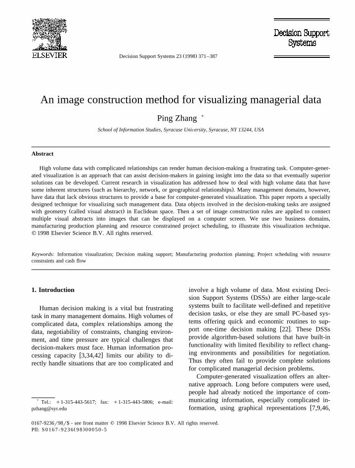
Ž .100% or 0 for shortfall value .Next, the planner may want to focus on a specific

PPL to learn more about satisfaction status for prod-ucts in that PPL. In Fig. 7, Products Satisfaction byPPLs, a detailed image of Product Satisfaction for aspecific PPL is zoomed in from Fig. 6. Each productis identified by its identification number and can beexamined individually. In this figure, we used thesame layout for time as in Figs. 5 and 6 and thenapplied standard graphing technique to lay out prod-uct ID and product satisfaction data objects. Forexample, the image shows that product P_35 has

Ž .problems the bars are not as high as 100% for allthe weeks except the last three, where there is nodemand on production of this product. A detailedanalysis may be necessary to find out why P_35 hasproblems.

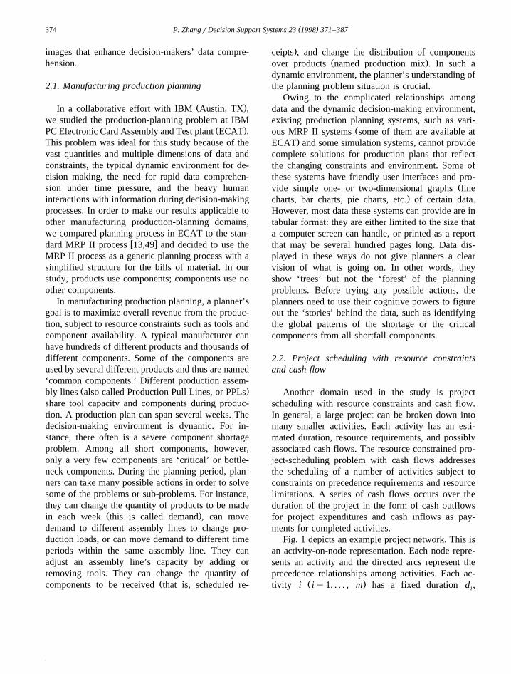
If a particular product is of great interest to theplanner, sherhe will want to know more about whatcauses problems for the production of this product.In production, all the required components have tobe in sets in order to produce one product. Fig. 8,Products Supported by Components, can provide adetailed view of which component of this product ismost lacking and thus affects the production of thisproduct. The underlined components at the right ofthe image are common components and are used bymultiple products. This image indicates to the plan-ner that sherhe should resolve the components withthe shortest bars before sherhe puts any effort onany other shortfall components. For example, theimage confirms that at week 1, C35_15 is the short-est component. It also shows that at week 2, al-though all the components are short for P_35, com-

Ž .ponents 1, 8 and 9 the shortest bars are among thecritical components and should be resolved first.Similar to those in Fig. 7, the different color barsmean there is no demand for Product 35 in weeks 10,

11, and 12. The technique for constructing the threedata objects is the same as that for Fig. 7.

4.2. Scheduling with SWAV

ŽWhen a project network is small, each node ac-.tivity is visible and thus the project is somehow

manageable. When the network becomes large, withhundreds or even thousands of nodes, the situation iscomplex, and it is almost impossible for the humanscheduler to trace each node, a subset of the net-work, or the entire network. The challenge is how torepresent an overall view of the entire network sothat without looking at the details at each node,schedulers are still able to see the potential bottle-necks or conflicts. After a bottleneck is identified, ascheduler may use his or her domain knowledge todevelop alternatives and take certain actions to re-duce or solve the problem. Among the many possibledirections for taking actions, which one to chooseremains a question. Meanwhile, there might be somedirectionsractions that the scheduler could not seedue to the complexity of the relationships and largevolume of data.

Fig. 9 depicts the status of critical factors in aŽ .schedule generated by a heuristic algorithm of a

Ž .project represented by Fig. 1 . These factors arecash inflows, outflows, and utilization of three re-

Žsources during the entire project life cycle 28 dura-.tion units . A human scheduler usually needs to

consider all these types of information in order toevaluate or refine a schedule. These factors arerepresented using standardized values; thus compar-isons are possible. Basically, the scheduler can useFig. 9, together with a diagram such as Fig. 1, toidentify some global patterns that are hidden in thedata or Fig. 1. For example, how do cash flowschange over time? What about resource utilizationchange overtime? What are the patterns of interac-tion among multiple data objects? Some patterns canbe used to guide the scheduler to take some actionsthat influence the entire project, not just neighbor-hood or segment of it. These global patterns providedirections for improving the schedule at a high level.This means that the scheduler does not need to lookat each activity in order to have the big picture of thecurrent schedule in terms of the critical factors.

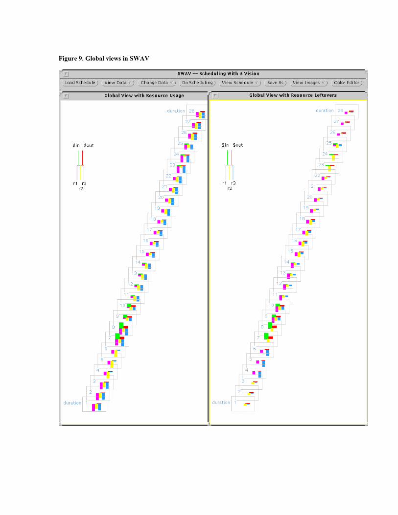
Figure 9. Global views in SWAV


Fig. 9. Global views in SWAV.

Fig. 9 has two mirror images indicating globalŽviews from both resource usage and leftover 100%-

.usage perspectives. By comparing these two images,

one may discover several patterns. For example,Ž .resource r blue bars is the best utilized among the3

three resources for most of the time. Resource r1


Ž . Ž .purple bars and r yellow bars are not fully2Žutilized in general except r for some periods such2

.as 1–3 and 23–24, and r for duration 4–6 . Inflows3Ž . Žgreen bars only happen during two periods dura-

. Ž .tion 7–14, and 23–25 , while outflows red bars arespread out evenly over the entire project life cycle.In this particular example, no special pattern orrelationship between changes of cash flows andchanges of resource utilization can be identified. Aconclusion to the current schedule is that it is notadjustable and is already the optimal schedule fromthe resource utilization perspective. Fig. 1 shows thatexcept node B, every node needs about half or moreof resource r . Fig. 9 leftover view shows that no3

Ž .duration except 4–6 for node B has more than halfof r left. Resource r is thus the bottleneck for this3 3

project.Ž .The visual abstract for the time concept duration

can be a little different if the number of durationbecomes extensive. Instead of using a continuousline segment, we could use groups of line segments

w xas the visual abstract for duration 57 . This is aspecial situation where each of the elements of a dataobject with an extensive number of elements has tobe identified. A similar approach can be found in

w xother research reports such as Refs. 1,51 .The construction of the images in Fig. 9 is based

Žon Rule 1 both inflows and outflows are dependent.on the utilization of the three resources and Rule 3

Žthe three resources are independent to each other,the inflows and outflows are independent to each

.other .

4.3. Systems eÕaluation

Even though this paper focuses on the develop-ment of visualization technique, a brief discussion ofsystem evaluation is appropriate. Studies of systemeffectiveness or usefulness can be conducted either

Žduring the system development process that is, for-. Žmative or after the system is finished that is, sum-. w xmative 36 . Evaluation methods include heuristics,

cognitive walkthrough, controlled experiment, sur-w xveys, interviews and focus groups 27,36,37,44 , to

name just a few.For Viz_planner, we used formative methods in-

cluding heuristics, cognitive walkthrough, and focusgroups of domain experts from two different manu-

facturing plants. These formative evaluations helpedus to refine the construction rules in order to con-struct effective images that are acceptable by thedomain users. When the prototype Viz_planner wasfinished, we conducted a controlled lab experimentusing 13 motivated subjects with production plan-ning background. The results show that visualization:Ž .1 helped generate more alternatives for solutions,Ž .2 helped make more efficient changes in the raw

Ž .data to achieve high-quality plans, and 3 madew xsubjects more satisfied with the outcomes 52,54 .

Although not every system requires a summativeevaluation, we plan to have an extended empiricalstudy in a real world setting in the future because itwill definitely provide a fuller understanding of thereal impact of VIZ_planner on manufacturing pro-duction-planning support.

SWAV has also gone through heuristic evalua-tion, cognitive walkthrough, and domain experts’evaluation of the current visual representations, whichare applications of the image construction methodintroduced in this paper. At present, SWAV focuseson general project scheduling problems with cashflows. We plan to apply SWAV to a specific busi-ness area for project scheduling and managementand to evaluate its usefulness using focus groups.

5. Conclusions

The current prototypes VIZ_planner and SWAVsupport static display of images, that is, changes todata need to be processed before changes show onthe images. Dynamic display or direct manipulationon images for changing raw data is under develop-ment. In both systems, the images are resizable inboth horizontal and vertical directions, and the anglefor the entire image changes correspondingly to en-sure clear readings. Users can also adjust colors to be

Žused in images either in a pre-run-time way inVIZ_planner, one needs to recompile the system in

.order to show the change of colors or run-timeŽ .fashion for SWAV . For example, in SWAV, a user

can change the color for any factors and see thechange immediately by using the color editor tool.

Information visualization is a powerful techniquewith tremendous potential for supporting complexdecision-making and problem-solving processes.


However, information visualization is still in its in-fancy and requires research exploration on specialtechniques, as well as more applications and evalua-tions. This is especially true for management infor-mation visualization. The current research adds valueto the information visualization area by testing thefeasibility of visualizing high volumes of seeminglynon-visual managerial data for decision-making sup-port. We intend to develop specific visualizationmethods based on the nature of managerial data, thedecision-making tasks, and human perceptional char-acteristics. In doing so, we hope that the process ofvisualizing managerial data for decision-making sup-port can become more science than art. We haveused two specific business domains for the presentstudy. We believe that what we have achieved con-tributes to our ultimate goals of developing visualiza-tion methods that can be applied to many manage-ment domains.

Acknowledgements

I thank Dr. Andrew B. Whinston and Dr. Peng SiOw for their contributions to the early stage of thisresearch. I thank my colleagues Drs. Kevin Crow-ston, Robert Heckman, and Steve Sawyer for theirhelpful remarks during the preparation of this paper.I thank the anonymous reviewers for their commentsand suggestions for finalizing this paper.

References

w x1 V. Anupam, S. Dar, T. Leibfried, E. Petajan, DataSpace: 3-Dvisualizations of large databases, in: Proceedings of IEEEInformation Visualization, 1995.

w x2 T. Asahi, D. Turo, B. Shneiderman, Using treemaps tovisualize the analytic hierarchy process, Information Systems

Ž . Ž .Research 6 4 1995 .w x3 R. Baecher, Grudin, Buxton, and Greenberg, Readings in

Human–Computer Interaction: Toward the Year 2000, 2ndedn., Morgan Kaufmann Publishers, 1995.

w x4 R.A. Becker, S.G. Eick, A.R. Wilks, Visualizing networkdata, IEEE Transactions on Visualization and Computer

Ž . Ž .Graphics 1 1 1995 .w x5 P.C. Bell, R.M. O’Keefe, An experimental investigation into

the efficacy of visual interactive simulation, ManagementŽ .Science 41 1995 .

w x6 I. Benbasat, A. Dexter, P. Todd, An experimental programinvestigating color-enhanced and graphics information pre-

Ž .sentation: an integration of the findings, CACM 29 11Ž .1986 .

w x7 J. Bertin, Semiology of Graphics, Translated by William J.Berg, The University of Wisconsin Press, 1983.

w x8 R. Bey, R.H. Doersch, J.H. Patterson, The net present valuecriterion: its impact on project scheduling, Project Manage-

Ž . Ž .ment Quarterly 12 2 1981 .w x9 W.C. Brinton, L.P. Ayres, N.A. Carle, R.E. Chaddock, Joint

committee on standards for graphic presentation, AmericanŽ .Statistical Association, New Series 112 1915 .

w x10 J. Carriere, R. Kazman, Interacting with huge hierarchies:beyond cone trees, in: Proceedings of the First IEEE Sympo-sium on Information Visualization, 1995.

w x11 H. Chernoff, The use of faces to represent points in k-dimen-sional space graphically, Journal of American Statistical

Ž .Association 68 1973 .w x12 W.S. Cleveland, Visualizing Data, Hobart Press, 1993.w x13 T.M. Cook, R.A. Russell, Contemporary Operations Manage-

ment, Prentice-Hall, 1980.w x14 F.E. Croxton, H. Stein, Graphic comparisons by bars, squares,

Ž .circles, and cubes, American Statistical Association 17 177Ž .1932 .

w x15 E. Davis, J.H. Patterson, A comparison of heuristic andoptimal solutions in resource-constrained project scheduling,

Ž . Ž .Management Science 21 8 1975 .w x16 T.A. DeFanti, M.D. Brown, B.H. McCormick, Visualization

—expending scientific and engineering research opportuni-ties, Computer, August 1989.

w x17 G. DeSanctis, Computer graphics as decision aids: directionsŽ .for research, Decision Sciences 15 1984 .

w x18 G. DeSanctis, S.L. Jarvenpaa, Graphical Presentation of Ac-counting Data for Financial Forecasting: An ExperimentalInvestigation, Accounting, Organizations, and Society 14Ž . Ž .5r6 1989 .

w x19 G. Dickson, G. DeSanctis, D.J. McBride, Understanding theeffectiveness of computer graphics for decision support: a

Ž . Ž .cumulative experimental approach, CACM 29 1 1986 .w x20 S.G. Eick, G.J. Wills, High interaction graphics, European

Ž .Journal of Operational Research 81 1995 .w x21 K.M. Fairchild, S.E. Poltrock, G.W. Furnas, SemNet: Three-

dimensional graphic representations of large knowledgeŽ .bases, in: R. Guindon Ed. , Cognitive Science and its Appli-

cations for Human–Computer Interaction, Lawrence ErlbaumAssociates, 1988.

w x22 L.R. Foulds, Layout manager: a microcomputer-based deci-sion support system for facilities layout, Decision Support

Ž .Systems 20 1997 .w x23 M.R. Garey, D.S. Johnson, Computers and Intractability: A

Guide to the Theory of NP-Completeness, Freeman, NewYork, 1979.

w x24 N. Gershon, S. Eick, Visualization’s New Tack: MakingSense of Information, IEEE Spectrum, November 1995.

w x25 R.D. Hurrion, Visual interactive modeling, European JournalŽ .of Operational Research 23 1986 .

w x26 S.L. Jarvenpaa, The effect of task demands and graphicalformat on information processing strategies, Management

Ž . Ž .Science 35 3 1989 .


w x27 R. Jeffries, J.R. Miller, C. Wharton, K.M. Uyeda, UserInterface evaluation in the real world: a comparison of fourtechniques, CHI’91 Proceedings, pp. 189–202.

w x28 C. Jones, An introduction to graph-based modeling systems:Ž . Ž .Part I. Overview, ORSA Journal on Computing 2 2 1990 .

w x29 C. Jones, An introduction to graph-based modeling systems:Part II. Graph-grammars and the implementation, ORSA

Ž . Ž .Journal on Computing 3 3 1991 .w x30 C. Jones, Visualization and optimization, ORSA Journal on

Ž . Ž .Computing 6 3 1994 .w x Ž .31 J.H. Larkin, H.A. Simon, Why a diagram is sometimes

Ž .worth ten thousand words, Cognitive Science 11 1987 .w x32 G.L. Lohse, K. Biolsi, N. Walker, H.H. Rueler, A classifica-

Ž . Ž .tion of visual representations, CACM 37 12 1994 .w x Ž .33 B.H. McCormick, et al. Eds. , Visualization in scientific

Ž . Ž .computing, Computer Graphics 22 6 1987 .w x34 G.A. Miller, The magical number seven, plus or minus two:

some limits on our capacity for processing information,Ž . Ž .Psychological Review 63 2 1956 .

w x35 A. Newell, H.A. Simon, Human Problem Solving, Prentice-Hall, 1972.

w x36 J. Nielsen, Usability Engineering, AP Professional, NewYork, 1993.

w x Ž .37 J. Nielsen, R. Mack Eds. , Usability Inspection Methods,Wiley, 1994.

w x38 H. Reuter, Human perception and visualization, in: Proceed-ings of the First IEEE Conference on Visualization, Visual-ization’90, 1990.

w x39 G. Robertson, S. Card, J. Mackinlay, Cone trees: animated3D visualizations of hierarchical information, in: Proceedingsof CHI’91, 1991.

w x40 L.J. Rosenblum, B. Brown, Visualization, IEEE ComputerGraphics and Applications, July 1992.

w x41 D.E. Rumelhart, D.A. Norman, Representations in memory,Ž .in: R.C. Atkinson, et al. Eds. , Stevens’ Handbook of Exper-

imental Psychology, 2nd edn., Vol. 2, Wiley, New York,1988.

w x42 R.M. Shiffrin, Capacity limitations in information process-Ž .ing, attention, and memory, in: W.K. Estes Ed. , Handbook

of Learning and Cognitive Processes, Vol. 4: Attention andMemory, Lawrance Erlbaum Associates, 1976.

w x43 B. Shneiderman, Tree visualization with tree-maps: a 2-Dspace-filling approach, ACM Transactions on Graphics 11Ž . Ž .1 1992 .

w x44 B. Shneiderman, Designing the User Interface: Strategies forEffective Human–Computer Interaction, 3rd edn., Addison-Wesley, 1997.

w x45 J.W. Tukey, Exploratory Data Analysis, Addison-Wesley,Reading, MA, 1977.

w x46 E.R. Tufte, Envisioning Information, Graphics Press,Cheshire, CT, 1990.

w x47 E.R. Tufte, The Visual Display of Quantitative Information,Graphics Press, Cheshire, CT, 1983.

w x48 I. Vessey, Cognitive fit: a theory-based analysis of the graphŽ .versus tables literature, Decision Sciences 22 1991 .

w x49 T.E. Vollmann, W.L. Berry, D. Clay Whybark, Manufactur-ing Planning and Control Systems, 2nd edn., Dow Jones-Irwin, Homewood, IL, 1988.

w x50 J.N. Washburne, An experimental study of various graphics,tabular, and textual methods of presenting quantitative mate-

Ž .rials, Journal of Educational Psychology 18 1927 .w x51 P. Wong, A. Crabb, R. Bergeron, Dual multiresolution hy-

perslice for multivariate data visualization, in: Proceedings ofIEEE Information Visualization, 1996.

w x52 P. Zhang, Visualization for decision-making support, PhDDissertation, The University of Texas at Austin, 1995.

w x53 P. Zhang, A.B. Whinston, Business information visualizationfor decision-making support: a research strategy, in: Proceed-ings of the First Americas Conference on Information Sys-tems, 1995.

w x54 P. Zhang, A comparative study of how information visualiza-tion affects human problem-solving performance in a com-plex business domain, in: Proceedings of Asia-Pacific DSIConference, 1996.

w x55 P. Zhang, Visualizing production planning data, IEEE Com-Ž . Ž .puter Graphics and Applications 16 5 1996 .

w x56 P. Zhang, J. Pick, Generating large data sets for simulation ofŽ . Ž .electronics manufacturing, Simulation 70 4 1998 .

w x57 P. Zhang, D. Zhu, Information visualization in project man-agement and scheduling, in: Proceedings of The 4th Confer-ence of the International Society for Decision Support Sys-

Ž .tems ISDSS97 , Switzerland, 1997.w x58 D. Zhu, R. Padman, Connectionist Approaches for Solver

Selection in Constrained Project Scheduling, the Annals ofOperations Research, 1997.

Ping Zhang is Assistant Professor atSchool of Information Studies, SyracuseUniversity. She has published papers inthe areas of information visualization,user interface studies, computer simula-tion, and technology-assisted education.She has received a teaching award fromUT Austin and a best paper award fromthe International Academy for Informa-tion Management. Dr. Zhang has a PhDin Information Systems from the Uni-versity of Texas at Austin, and MSc and

BSc in Computer Science from Peking University, Beijing, China.Dr. Zhang is a member of the ACM SIGCHI, IEEE ComputerSociety, INFORMS, AIS, and IAIM.

An image construction method for visualizing managerial...

Documents

Transcript of An image construction method for visualizing managerial...