An Identity Crisis for the Casimir Operator

Thomas R. LoveDepartment of Mathematics

andDepartment of Physics

California State University, Dominguez HillsCarson, CA, 90747tlove@csudh.edu

April 16, 2006

Abstract

The Casimir operator of a Lie algebra L is C2 =∑

gijXiXj andthe action of the Casimir operator is usually taken to be C2Y =∑

gijXiXjY , with ordinary matrix multiplication. With this defini-tion, the eigenvalues of the Casimir operator depend upon the repre-sentation showing that the action of the Casimir operator is not welldefined. We prove that the action of the Casimir operator shouldbe interpreted as C2Y =

∑gij [Xi, [Xj ,Y ]]. This intrinsic definition

does not depend upon the representation. Similar results hold for thehigher order Casimir operators. We construct higher order Casimiroperators which do not exist in the standard theory including a newtype of Casimir operator which defines a complex structure and thirdorder intrinsic Casimir operators for so(3) and so(3, 1). These opera-tors are not multiples of the identity. The standard theory of Casimiroperators predicts neither the correct operators nor the correct num-ber of invariant operators. The quantum theory of angular momentumand spin, Wigner’s classification of elementary particles as represen-tations of the Poincare Group and quark theory are based on faultymathematics. The “no-go theorems” are shown to be invalid.

PACS 02.20S

1

1 Introduction

Lie groups and Lie algebras play a fundamental role in classical mechan-ics, electrodynamics, quantum mechanics, relativity, and elementary particlephysics. Many hope that the Lie group/algebra setting will provide an ap-propriate framework for the unification of quantum theory, general relativ-ity and particle physics. Within the unification via group theory program,the so-called Casimir operators or invariant operators play a pivotal role.In quantum mechanics, the quadratic Casimir operator of so(3) is eitherL2, the total angular momentum or J2, the total spin. In the program ofdynamical groups or spectrum generating algebras, the eigenvalues of theCasimir operators can be interpreted as mass, energy, momentum, or otherdynamical quantities. H. Schwartz [28] emphasized the role of the Casimiroperator in Relativity, while W. Greiner and B. Muller [7] emphasized therole of the Casimir operator in quantum mechanics. Thus it seems likelythat the Casimir operators of some Lie algebra will play a major role in theunification of the two theories. The author [17] suggested that u(3, 2) is theunique Lie algebra capable of such a unification. A Theory of Matter basedon the geometry of u(3, 2) was developed in Love [18, 19, 20]. In this pro-gram, the field equations arise as eigenvalue equations involving the Casimiroperators of u(3, 2), with the conserved quantities as the eigenvalues. Thusidentification of the proper operators is essential to progress in the TheoryOf Matter.

A Casimir operator, C, of a Lie Algebra L is an operator constructed asa polynomial in the elements of L which commutes with every element of L.With an abuse of notation, this is written as

[C, X] = 0 ∀X ∈ L.

This is an abuse of notation because the bracket is use to denote the operationdefined on the Lie algebra so writing [A, B] = 0 implies that both A and Bare in the Lie algebra. The Casimir operator is not in the Lie algebra itself,rather the Casimir operator is in the Enveloping algebra of the Lie algebra.So

[C, X] = 0

really means that CXY = XCY , but this equation makes no sense in a Liealgebra since the product XY is not defined, only the bracket is defined.Putting brackets in, we have: [CX, Y ] = [X, CY ], or should it be C[X, Y ] =[X, CY ]? We need to examine this issue.

2

We begin with Schur’s lemma as phrased in Proposition 2 of Chevalley[3]:

Let P be an irreducible representation of a group G in analgebraically closed field K. The only matrices which commutesimultaneously with all matrices P (σ), σ ∈ G are the scalar mul-tiples of the unit matrix. (page 183)

In many treatments of the Casimir operator, an appeal is made to Schur’sLemma to show that the Casimir operator (and every generalized Casimiroperator) is a multiple of the identity matrix. As we will show, this statementas it stands is not true. In the context of representation by differentialoperators, the phrase doesn’t even make sense. We will show that Schur’sLemma is not true for differential operator representations of Lie algebras.

Suppose that each element of a Lie algebra is an eigenvector of the Casimiroperator C of the Lie algebra L, thus:

CX = αX ∀X ∈ L (1)

Now let ρ be an isomorphism of the Lie Algebra L and apply ρ to bothsides of (1) to obtain:

ρ(CX) = ρ(αX) (2)

Commutivity of the diagram:

L C−→ L

ρ ↓ ρ ↓ρ(L) ρ(C)

−→ ρ(L)

requires that:ρ(CX) = ρ(C)ρ(X)

In the representation space we have:

ρ(C)ρ(X) = αρ(X).

In order to be a scalar, α must be the same in all representations (that is thedefinition of scalar). In the standard approach, with

C =∑

gijXiXj

3

andCY =

∑gijXiXjY

for Y ∈ L for consistency we must have:

ρ(C2)ρ(Y ) =∑

gijρ(Xi)ρ(Xj)ρ(Y )

But this is not the case, as the examples considered by Schiff [26] show. Schiffasserts (p. 199): “Direct substitution from the matrices (27.11) shows that

S2 = S2x + S2

y + S2z

is equal to 2h2 times the unit matrix”. This is indeed true, if we just multiplythe matrices (recall that physicists put in a factor of i to make the matrixhermitean):

Sx = ih

0 0 00 0 −10 1 0

Sy = ih

0 0 10 0 0−1 0 0

Sz = ih

0 1 0−1 0 00 0 0

Then we have:

S2A = S2xA + S2

yA + S2zA = 2hA

A ∈ so(3)

This calculation also ‘proves’ that S2A = 2hA for any three by threematrix, and in particular for A ∈ su(3). Consequently, if this proof werevalid, S2 would be a Casimir operator for su(3), sl(3) and any other Liealgebra of 3 by 3 matrices which contains so(3). It is not. Thus, the ‘proof’is not valid.

Switching representations, Schiff contends on page 203 that

Jx =h

2

(0 11 0

)

4

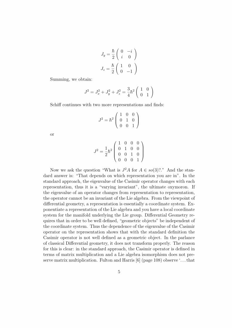
Jy =h

2

(0 −ii 0

)

Jz =h

2

(1 00 −1

)Summing, we obtain:

J2 = J2x + J2

y + J2z =

3

4h2

(1 00 1

)

Schiff continues with two more representations and finds:

J2 = h2

1 0 00 1 00 0 1

or

J2 =1

2h2

1 0 0 00 1 0 00 0 1 00 0 0 1

Now we ask the question “What is J2A for A ∈ so(3)?.” And the stan-

dard answer is: “That depends on which representation you are in”. In thestandard approach, the eigenvalue of the Casimir operator changes with eachrepresentation, thus it is a “varying invariant”, the ultimate oxymoron. Ifthe eigenvalue of an operator changes from representation to representation,the operator cannot be an invariant of the Lie algebra. From the viewpoint ofdifferential geometry, a representation is essentially a coordinate system. Ex-ponentiate a representation of the Lie algebra and you have a local coordinatesystem for the manifold underlying the Lie group. Differential Geometry re-quires that in order to be well defined, “geometric objects” be independent ofthe coordinate system. Thus the dependence of the eigenvalue of the Casimiroperator on the representation shows that with the standard definition theCasimir operator is not well defined as a geometric object. In the parlanceof classical Differential geometry, it does not transform properly. The reasonfor this is clear: in the standard approach, the Casimir operator is defined interms of matrix multiplication and a Lie algebra isomorphism does not pre-serve matrix multiplication. Fulton and Harris [6] (page 108) observe ‘. . . that

5

the “composition” X Y of elements of a Lie algebra is not well defined.’In order to be well defined within the category of Lie algebras, the action ofthe Casimir operator cannot be defined in terms of matrix multiplication, itmust be defined in terms of the Lie bracket.

Consequently, although the standard results about the Casimir operatorfollow from direct calculation, those calculations are meaningless from a ge-ometric (or a categorical) viewpoint. Our immediate goal must be to finda way of defining the Casimir operator in a way which is geometrically andcategorically satisfactory.

We begin by looking at the geometric origin of the Lie bracket. LetF (t) be the flow of the vector field X and F ∗ the pullback map under thediffeomorphism induced by that flow, then the Lie derivative of a tensor fieldK with respect to the vector field X is defined by

LXK(p) = limt→0

(K(p)− F ∗(t)K(p))/t

It is a standard exercise in differential geometry to prove that the Liederivative of a vector field Y with respect to another vector field X is givenby:

LXY = [X, Y ] = XY − Y X

(Kobayashi and Nomizu [14],p.29).Within differential geometry, the commutator is then a secondary tool

used to compute the Lie brackets. Any computations using a matrix repre-sentation of a Lie algebra which comes from a Lie group must be consistantwith the geometric origin of the Lie derivative, matrix multiplication is not.The reader interested in more detail should read the entire discussion of thematter in Fulton and Harris [6].

In the standard approach, the Casimir operator for a Lie algebra L , is

C2 =∑

gijXiXj (3)

and the action of the Casimir operator is

C2Y =∑

gijXiXjY (4)

with ordinary matrix multiplication. However, matrix multiplication is notdefined in a Lie algebra, only the Lie bracket, addition and scalar multi-plication are defined. Since a Lie Algebra with the bracket operation isnonassociative, this expression is meaningless. Since the action (4) is not

6

well defined, we look for other ways to interpret the symbols. In anotherstandard treatment, the Casimir operator is taken to be an element of theEnveloping Algebra in which case

C2Y =∑

gijXi ⊗Xj⊗Y

with the tensor product as the multiplication. We will look at this treatmentafter discussing yet another way to interpret the symbols.

Since the Casimir operator is defined in terms of the generators of theLie algebra and the generators are defined in terms of the Lie derivative, itseems appropriate to have the Casimir operators defined in terms of the Liederivative.

Kobayashi and Nomizu [15](p.128) prove that a vector field X is an in-finitesimal automorphism of an almost complex structure J iff

J [X, Y ] = [X, JY ]

Phrased another way, this condition insures the almost complex structureJ is invariant under the flow generated by the vector field X. This theorem isrelevant since we will construct a Casimir operator which defines a complexstructure. We can use their proof verbatim, replacing J by C to prove:

Theorem:Given a Lie Algebra L , if C :→ L is a linear operator, then C is invariant

under the flow generated by the vector field X, iff

C[X, Y ] = [X, CY ] = [CX, Y ] (5)

for all X,Y ∈ L .Proof:Consider the Lie algebra as the tangent space of M , the manifold under-

lying the Lie group. Then the Casimir operator is a mapping

C : TM → TM.

Let X and Y be any vector fields on M . Then

[X, CY ] = LX(CY ) = (LXC)Y + CLX(Y ) = (LXC)Y + C[X, Y ]

Hence, LXC = 0 iff[X, CY ] = C[X, Y ].

7

The condition that the Lie derivative of C with respect to X is zero, LXC = 0is the definition of invariant.

Then we also have

C[X, Y ] = −C[Y, X] = −[Y,CX] = [CX, Y ]

The standard approach requires that CX = XC, or putting in anotherelement Y for these operators to act on, the standard approach requires thatC commutes with X under the operation of matrix multiplication:

CXY = XCY (6)

In the approach taken here, we require that C interacts with X under theoperation of the Lie algebra, the Lie bracket and thus:

C[X, Y ] = [X,CY ] (7)

Again, the standard approach cannot be correct simply because matrixmultiplication is not defined in a Lie Algebra. This is a different interpre-tation of the phrase “commutes with X” than the standard theory and isjustified because it is local invariance under the action of the Lie algebrawhich leads to global invariance under the action of the Lie Group.

TheoremIn any representation, the action of the Casimir operator C is given by

CY =∑

gij[Xi, [Xj, Y ]] (8)

Proof:In the standard treatment of the Casimir operator, C ,

CXk =∑ij

gijXiXjXk

In the adjoint representation, we have the Casimir operator acting on anelement of the Lie algebra:

CA =∑ij

gijad(Xi)ad(Xj)A

then, by definition of the adjoint representation,

(adC)(adA) =∑ij

gij[adXi, [adXj, adA]]

8

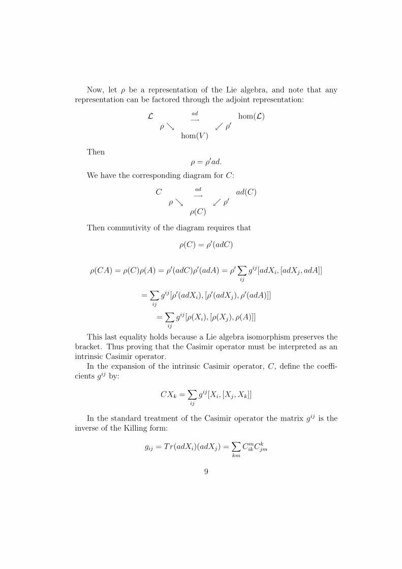
Now, let ρ be a representation of the Lie algebra, and note that anyrepresentation can be factored through the adjoint representation:

L ad−→ hom(L)

ρ ρ′

hom(V )

Thenρ = ρ′ad.

We have the corresponding diagram for C:

C ad−→ ad(C)

ρ ρ′

ρ(C)

Then commutivity of the diagram requires that

ρ(C) = ρ′(adC)

ρ(CA) = ρ(C)ρ(A) = ρ′(adC)ρ′(adA) = ρ′∑ij

gij[adXi, [adXj, adA]]

=∑ij

gij[ρ′(adXi), [ρ′(adXj), ρ

′(adA)]]

=∑ij

gij[ρ(Xi), [ρ(Xj), ρ(A)]]

This last equality holds because a Lie algebra isomorphism preserves thebracket. Thus proving that the Casimir operator must be interpreted as anintrinsic Casimir operator.

In the expansion of the intrinsic Casimir operator, C, define the coeffi-cients gij by:

CXk =∑ij

gij[Xi, [Xj, Xk]]

In the standard treatment of the Casimir operator the matrix gij is theinverse of the Killing form:

gij = Tr(adXi)(adXj) =∑km

CmikCk

jm

9

However, with the reinterpretation of the Casimir operator, this relation-ship is not valid. As a direct calculation with the normalized intrinsic Casimiroperator shows:

CXk =∑ij

gij[Xi, [Xj, Xk]]

=∑ij

gij[Xi,∑

l

C ljkXl]

=∑ijl

gij[Xi, CljkXl]

=∑ijl

gijC ljk[Xi, Xl]

=∑ijlm

gijC ljkC

mil Xm

Denote the inverse of gij by hjk then the relation between a matrix andits inverse is given by

gijhjk = δik

and is summed over the index j only. Since the expression

∑ijlm

gijC ljkC

mil Xm (9)

is summed over both i and j, the relation between gij and C ljkC

mil is not that

between a matrix and its inverse.O’Raifeartaigh [24] claimed that the Casimir operator could be written

as

CXk =∑ij

Tr(adXi)(adXj)[Xi, [Xj, Xk]].

However, this expression cannot be correct since Tr(adXi)(adXj) is theKilling form and according to the standard formula, it is the inverse of theKilling form which defines the coefficients of the Casimir operator. But (9)shows that this doesn’t work. Instead of taking the inverse of the matrix, weneed to take the inverse of each term individually and define:

10

CXk =∑ij

( Tr(adXi)(adXj) )−1 [Xi, [Xj, Xk]]. (10)

(The sum is over nonzero traces)O’Raifeartaigh’s calculations work out because he only considers cases

where Tr(adXi)(adXj) is 1 or -1.Note that (adXi)(adXj) = [Xi, [Xj, ; so we could write:

CXk =∑ij

(Tr[Xi, [Xj, )−1[Xi, [Xj, Xk]] (11)

(The sum is over nonzero traces)We will call the operator defined in (10) the normalized intrinsic Casimir

operator. With a slight change of notation, this agrees with the definitionof the Casimir operator given by Knapp [13]. This operator is scale invari-ant, that is, if each Xi is multiplied by a scalar ai, the normalized intrinsicCasimir operator is unchanged (in the standard picture, this is only true foran orthogonal basis). Such rescalings will be necessary to properly scale fieldstrengths [31].

The intrinsic Casimir operator is one of the invariants of the Lie algebra.When we speak of invariants in differential geometry, we mean a differentialoperator which is invariant under the action of the Lie Group. This imme-diately leads to the criteria that in the representation of the Lie algebra asdifferential operators the invariant operator commutes with elements of theLie algebra as in Theorem 5. But here arises the main point of confusionwhen we work with a matrix representation. If we want an operator whichcommutes with every element of the Lie algebra, does that mean that the op-erator commutes with the matrices in some representation under the actionof ordinary matrix multiplication or that the operator commutes with the ac-tion of that matrix as an element of the Lie algebra? The standard approachtakes the first route and requires that the operator commutes with everymatrix in the representation. Then, supposedly Schur’s lemma requires thatthese “invariant operators” are just multiples of the unit matrix. But thenthe “invariants” are a different multiple of the identity for each representa-tion and can hardly be called “invariant”. Noting that matrix multiplicationis not defined in a Lie algebra, we take the second tack and require thatthe operator commute with the action of the matrices as elements of the Liealgebra, as required by Theorem 5. The eigenvalue of these operators does

11

not change with the representation and they are truly invariant. We willalso show that the invocation of Schur’s lemma is not justified since theseoperators are not representable by matrix operators.

Since this approach is such a break with tradition, perhaps further dis-cussion is warranted. If A is an element of the Lie algebra of a Lie group,then A is the infinitesimal generator of a one parameter subgroup with thegroup action on B ∈ L given by: exp(tA)Bexp(−tA)

In order to prove the invariance of an operator C we need to show that:

Cexp(tA)Bexp(−tA) = exp(tA)(CB)exp(−tA)

Using the Baker-Campbell-Hausdorff identity, we can expand the groupaction in terms of the Lie algebra action:

exp(tA)Bexp(−tA) = (B + t[A, B] +t2

2![A, [A, B]] +

t3

3![A, [A, [A, B]]] + . . .

Then

exp(tA)(CB)exp(−tA) = (CB+t[A, CB]+t2

2![A, [A, CB]]+

t3

3![A, [A, [A, CB]]]+. . .

= (CB + Ct[A, B] + Ct2

2![A, [A, B]] + C

t3

3![A, [A, [A, B]]] + . . .

= C(B + t[A, B] +t2

2![A, [A, B]] +

t3

3![A, [A, [A, B]]] + . . .)

= Cexp(tA)Bexp(−tA)

An invariant operator is one whose action commutes with that of theLie Group. The above calculation shows that in order for an operator tocommute with the action of the Lie group, it must commute with the actionof the Lie algebra in the sense of 5.

2 The Lie Algebra of Vectors and The Intrin-

sic Casimir Operator of so(3)

Consider the Lie Algebra of vector fields on R3 with bracket defined by crossproduct:

~i×~i = ~0 ~j ×~i = −~k ~k ×~i = ~j~i×~j = ~k ~j ×~j = ~0 ~k ×~j = −~i

~i× ~k = −~j ~j × ~k =~i ~k × ~k = ~0

12

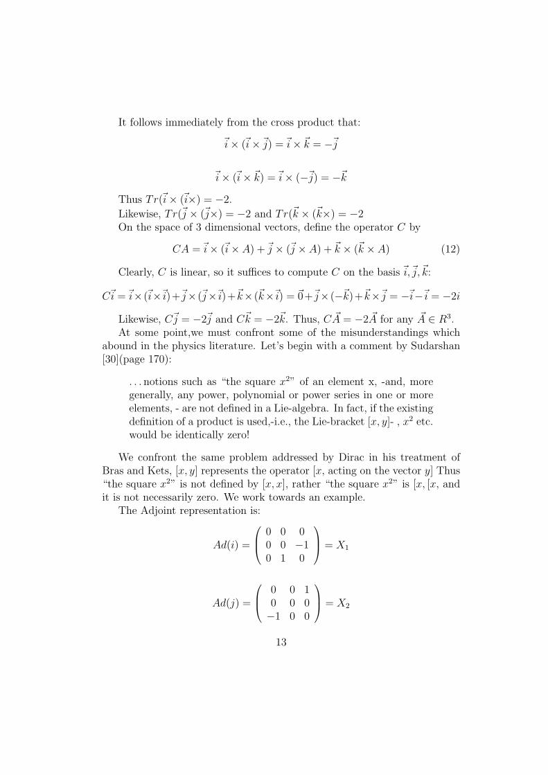
It follows immediately from the cross product that:

~i× (~i×~j) =~i× ~k = −~j

~i× (~i× ~k) =~i× (−~j) = −~k

Thus Tr(~i× (~i×) = −2.

Likewise, Tr(~j × (~j×) = −2 and Tr(~k × (~k×) = −2On the space of 3 dimensional vectors, define the operator C by

CA =~i× (~i× A) +~j × (~j × A) + ~k × (~k × A) (12)

Clearly, C is linear, so it suffices to compute C on the basis ~i,~j,~k:

C~i =~i× (~i×~i)+~j× (~j×~i)+~k× (~k×~i) = ~0+~j× (−~k)+~k×~j = −~i−~i = −2i

Likewise, C~j = −2~j and C~k = −2~k. Thus, C ~A = −2 ~A for any ~A ∈ R3.At some point,we must confront some of the misunderstandings which

abound in the physics literature. Let’s begin with a comment by Sudarshan[30](page 170):

. . . notions such as “the square x2” of an element x, -and, moregenerally, any power, polynomial or power series in one or moreelements, - are not defined in a Lie-algebra. In fact, if the existingdefinition of a product is used,-i.e., the Lie-bracket [x, y]- , x2 etc.would be identically zero!

We confront the same problem addressed by Dirac in his treatment ofBras and Kets, [x, y] represents the operator [x, acting on the vector y] Thus“the square x2” is not defined by [x, x], rather “the square x2” is [x, [x, andit is not necessarily zero. We work towards an example.

The Adjoint representation is:

Ad(i) =

0 0 00 0 −10 1 0

= X1

Ad(j) =

0 0 10 0 0−1 0 0

= X2

13

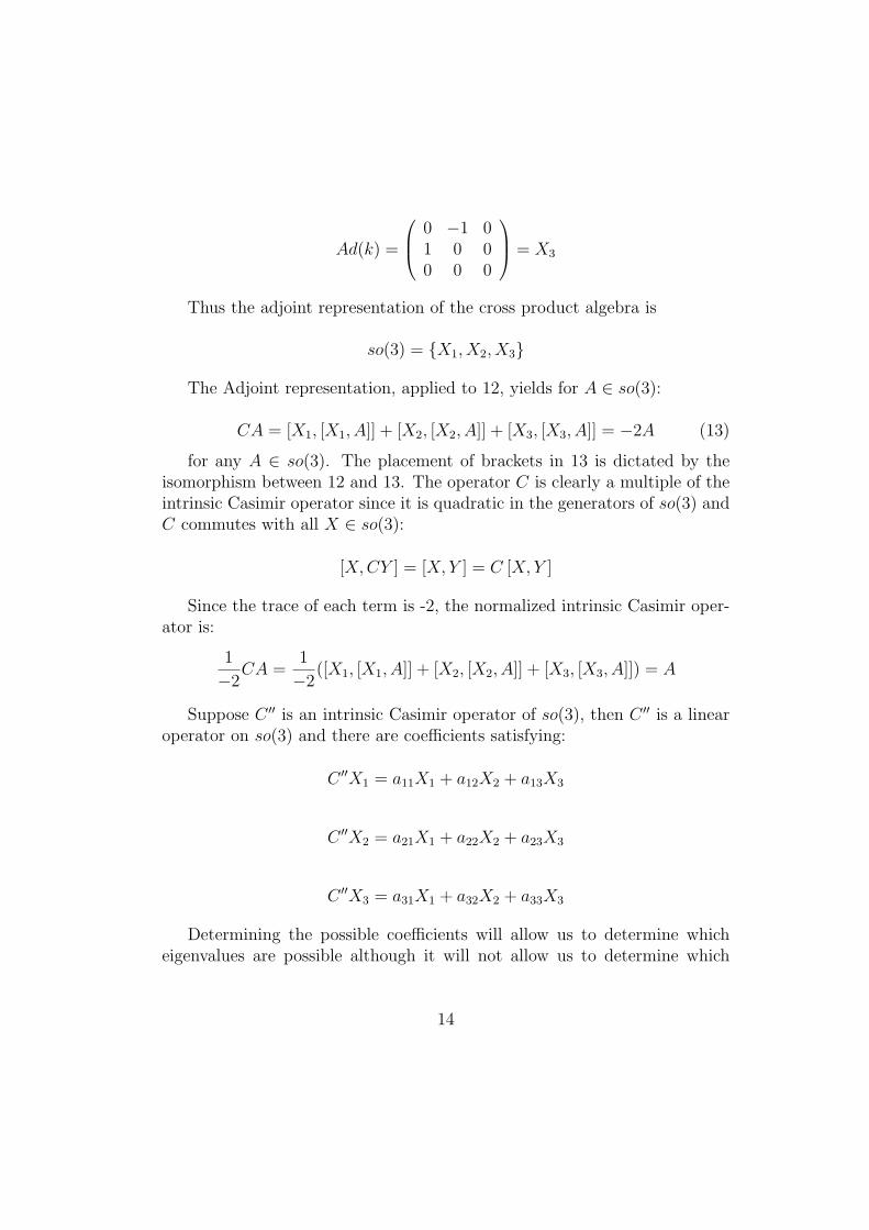
Ad(k) =

0 −1 01 0 00 0 0

= X3

Thus the adjoint representation of the cross product algebra is

so(3) = X1, X2, X3

The Adjoint representation, applied to 12, yields for A ∈ so(3):

CA = [X1, [X1, A]] + [X2, [X2, A]] + [X3, [X3, A]] = −2A (13)

for any A ∈ so(3). The placement of brackets in 13 is dictated by theisomorphism between 12 and 13. The operator C is clearly a multiple of theintrinsic Casimir operator since it is quadratic in the generators of so(3) andC commutes with all X ∈ so(3):

[X, CY ] = [X,Y ] = C [X, Y ]

Since the trace of each term is -2, the normalized intrinsic Casimir oper-ator is:

1

−2CA =

1

−2([X1, [X1, A]] + [X2, [X2, A]] + [X3, [X3, A]]) = A

Suppose C ′′ is an intrinsic Casimir operator of so(3), then C ′′ is a linearoperator on so(3) and there are coefficients satisfying:

C ′′X1 = a11X1 + a12X2 + a13X3

C ′′X2 = a21X1 + a22X2 + a23X3

C ′′X3 = a31X1 + a32X2 + a33X3

Determining the possible coefficients will allow us to determine whicheigenvalues are possible although it will not allow us to determine which

14

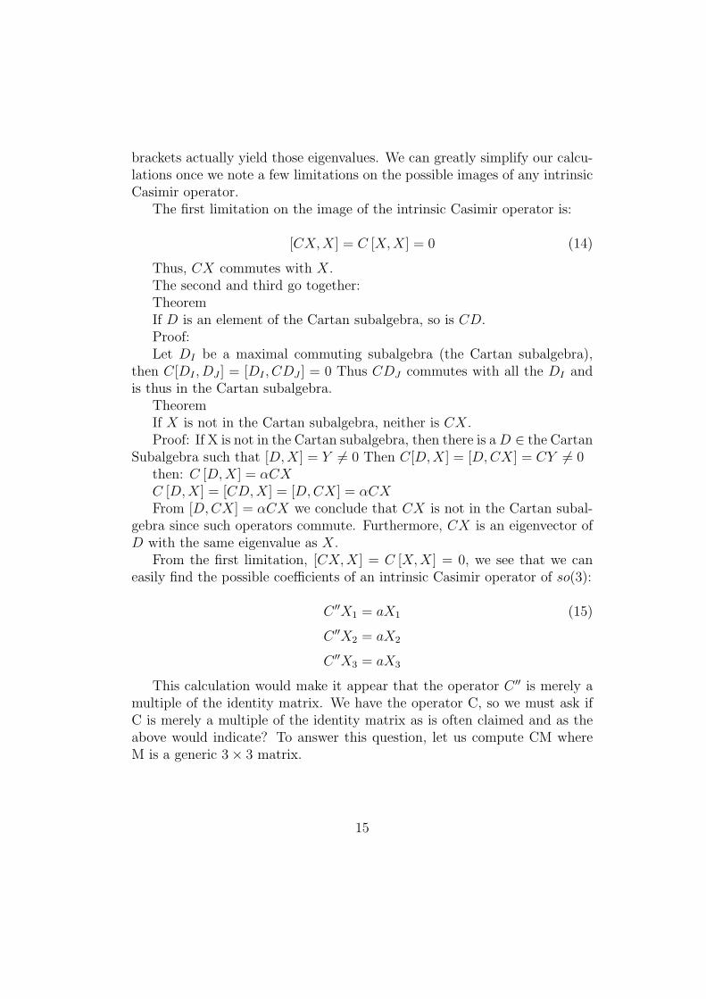
brackets actually yield those eigenvalues. We can greatly simplify our calcu-lations once we note a few limitations on the possible images of any intrinsicCasimir operator.

The first limitation on the image of the intrinsic Casimir operator is:

[CX, X] = C [X, X] = 0 (14)

Thus, CX commutes with X.The second and third go together:TheoremIf D is an element of the Cartan subalgebra, so is CD.Proof:Let DI be a maximal commuting subalgebra (the Cartan subalgebra),

then C[DI , DJ ] = [DI , CDJ ] = 0 Thus CDJ commutes with all the DI andis thus in the Cartan subalgebra.

TheoremIf X is not in the Cartan subalgebra, neither is CX.Proof: If X is not in the Cartan subalgebra, then there is a D ∈ the Cartan

Subalgebra such that [D, X] = Y 6= 0 Then C[D, X] = [D, CX] = CY 6= 0then: C [D, X] = αCXC [D, X] = [CD,X] = [D, CX] = αCXFrom [D, CX] = αCX we conclude that CX is not in the Cartan subal-

gebra since such operators commute. Furthermore, CX is an eigenvector ofD with the same eigenvalue as X.

From the first limitation, [CX, X] = C [X, X] = 0, we see that we caneasily find the possible coefficients of an intrinsic Casimir operator of so(3):

C ′′X1 = aX1 (15)

C ′′X2 = aX2

C ′′X3 = aX3

This calculation would make it appear that the operator C ′′ is merely amultiple of the identity matrix. We have the operator C, so we must ask ifC is merely a multiple of the identity matrix as is often claimed and as theabove would indicate? To answer this question, let us compute CM whereM is a generic 3× 3 matrix.

15

[X1, M ] =

0 0 0

0 0 −10 1 0

,

m11 m12 m13

m21 m22 m23

m31 m32 m33

0 0 0−m31 −m32 −m33

m21 m22 m23

− 0 m13 −m12

0 m23 −m22

0 m33 −m32

= 0 −m13 m12

−m31 −m23 −m32 m22 −m33

m21 m22 −m33 m23 + m32

Then

[X1, [X1, M ]] =

0 0 0

0 0 −10 1 0

,

0 −m13 m12

−m31 −m23 −m32 m22 −m33

m21 m22 −m33 m23 + m32

=

0 −m12 −m13

−m21 −2m22 + 2m33 −2m23 − 2m32

−m31 −2m23 − 2m32 2m22 − 2m33

Likewise:

[X2, [X2, M ]] =

2m33 − 2m11 −m12 −2m13 − 2m31

−m21 0 −m23

−2m31 − 2m13 −m32 −2m33 + 2m11

[X3, [X3, M ]] =

−2m11 + 2m22 −2m12 − 2m21 −m13

−2m12 − 2m21 2m11 − 2m22 −m23

−m31 −m32 0

Summing, we obtain:

CM =

−4m11 + 2m22 + 2m33 −4m12 − 2m21 −4m13 − 2m31

−4m12 − 2m12 2m11 − 4m22 + 2m33 −4m23 − 2m32

−4m31 − 2m13 −2m23 − 4m32 2m11 + 2m22 − 4m33

16

Thus C is not a multiple of the identity matrix, but the operator C has aneigenvalue of -2 which we need to investigate. Requiring that CM = −2M ,we have for the off diagonal terms:

2m12 + m21 = m12

Therefore,m12 = −m21

2m13 + m31 = m13

Therefore,m13 = −m31

2m23 + m32 = m23

It follows thatm23 = −m32

For the diagonal terms:

2m11 −m22 −m33 = m11

−m11 + 2m22 −m33 = m22

−m11 −m22 + 2m33 = m33

This system has only the solution m11 = m22 = m33 = 0Thus CM = −2M iff M is skew-symmetric, i.e. iff M ∈ so(3)! Hence, in

the defining representation, the intrinsic Casimir operator of so(3) charac-terizes the Lie algebra. This also happens to be the adjoint representation,so it is not clear which is important.

WritingC = ([X1)

2 + ([X2)2 + ([X3)

2

Then it is clear that

C = ([X1)2n + ([X2)

2n + ([X3)2n

is also a Casimir operator for any n. Similiar remarks hold for every Casimiroperator we will construct.

17

3 Third Order Intrinsic Casimir Operators

for so(3)

In this section we construct third order intrinsic Casimir operators for so(3),contrary to the standard wisdom in which so(3) has no third order Casimiroperators. Once again, we begin with the Lie Algebra of vectors on R3 withthe cross product as bracket.

~i× (~j × (~k ×~i)) = 0 (16)

~k × (~i× (~j ×~i))

= ~k × (~i× (−~k))

= ~k ×~j = −~i

~j × (~k × (~i×~i)) = 0

~i× (~j × (~k ×~j)) (17)

=~i× (~j × (−~i))

=~i× ~k = −~j

~k × (~i× (~j ×~j)) = 0

~j × (~k × (~i×~j)) = 0

~i× (~j × (~k × ~k)) = 0 (18)

~k × (~i× (~j × ~k)) = 0

~j × (~k × (~i× ~k)) = ~j × (~k × (−~j))

= ~j ×~i = −~k

Define for ~A ∈ R3,

C3−

~A =~i× (~j × (~k × ~A)) + ~k × (~i× (~j × ~A)) +~j × (~k × (~i× ~A))

It follows immediately that

C3−

~A = − ~A.

18

Now reverse the order of ~i,~j, and ~k:

~k × (~j × (~i×~i)) = 0 (19)

~i× (~k × (~j ×~i)) = 0

~j × (~i× (~k ×~i)) = ~j × (~i×~j)

= ~j × ~k =~i

~k × (~j × (~i×~j)) = ~k × (~j × ~k) (20)

= ~k ×~i = ~j

~i× (~k × (~j ×~j)) = 0

~j × (~i× (~k ×~j)) = 0

~k × (~j × (~i× ~k)) = 0 (21)

~i× (~k × (~j × ~k)) =~i× (~k ×~i)

=~i×~j = ~k

~j × (~i× (~k × ~k)) = 0

Define for ~A ∈ R3

C3+

~A = ~k × (~j × (~i× ~A)) +~i× (~k × (~j × ~A)) +~j × (~i× (~k × ~A)) (22)

It follows immediately that C3+

~A = ~A. Furthermore, note that the samecalculations show that the three terms of this operator are the projectionoperators, if ~A = A1

~i + A2~j + A3

~k then

~j × (~i× (~k × ~A)) = A1~i

~k × (~j × (~i× ~A)) = A2~j

~i× (~k × (~j × ~A)) = A3~k

19

Passing to the adjoint representation, we have for A ∈ so(3)

C3−A = [X1, [X2, [X3, A]]] + [X3, [X1, [X2, A]]] + [X2, [X3, [X1, A]]] = −A

and

C3+A = [X3, [X2, [X1, A]]] + [X1, [X3, [X2, A]]] + [X2, [X1, [X3, A]]] = A

Thus C3− and C3

+ are third order intrinsic Casimir operators of eigenvaluetype for so(3). But according to the standard treatment of higher orderCasimir elements, so(3) should not have any third order Casimir operatorswhich are not multiples of the second order operator. Thus the standardtreatment of higher order Casimir operators is fundamentally flawed.

The discovery of these third order operators was accomplished by whatappears to be a systematic way to construct candidate third order invariantsfor any Lie algebra, beginning with the second order invariant:

L2Y = [X1, [X1, Y ]] + [X2, [X2, Y ]] + [X3, [X3, Y ]]

In the term [X1, [X1, Y ]], for the first X1, use the substitution: X1 =[X2, X3]

Thus[X1, [X1, Y ]] = [[X2, X3], [X1, Y ]]

Now when we ask how this term could have arisen from the Jacobi identityin a third order operation we are led to consider the operator:

[X2, [X3, [X1, Y ]]]

In the term [X2, [X2, Y ]], for the first[X2, use the substitution:

X2 = [X3, X1]

Thus[X2, [X2, Y ]] = [[X3, X1], [X2, Y ]]

This term could have arisen from the Jacobi identity in a third orderoperation:

[X3, [X1, [X2, Y ]]] = [[X3, X1], [X2, Y ]] + [X1, [X3, [X2, Y ]]]

20

= [X2, [X2, Y ]] + [X1, [X3, [X2, Y ]]]

In the term [X3, [X3, Y ]], for the first [X3, use the substitution:

X3 = [X1, X2]

Thus[X3, [X3, Y ]] = [[X1, X2], [X3, Y ]]

This term could have arisen from the Jacobi identity from an expansionof the operator:

[X1, [X2, [X3, Y ]]] = [[X1, X2], [X3, Y ]] + [X2, [X1, [X3, Y ]]]

= [X3, [X3, Y ]] + [X2, [X1, [X3, Y ]]]

Now we sum the three operators:

[X1, [X2, [X3, Y ]]] + [X2, [X3, [X1, Y ]]] + [X3, [X1, [X2, Y ]]]

Which we recognize as the operator:

C3−Y = [X1, [X2, [X3, Y ]]] + [X3, [X1, [X2, Y ]]] + [X2, [X3, [X1, Y ]]]

which we have already shown is an invariant. We could also use this methodto arrive at:

C3+Y = [X3, [X2, [X1, Y ]]] + [X2, [X1, [X3, Y ]]] + [X1, [X3, [X2, Y ]]]

We compute the action on a generic three by three matrix:

C3+M = [X3, [X2, [X1, M ]]] + [X2, [X1, [X3, M ]]] + [X1, [X3, [X2, M ]]]

by calculating each term separately.For the first term, we first calculate

[X2, [X1, M ]]

=

0 0 1

0 0 0−1 0 0

,

0 −m13 m12

−m31 −m23 −m32 m22 −m33

m21 m22 −m33 m23 + m32

=

21

m21 + m12 m22 −m33 m23 + m32

m22 −m33 0 m31

m23 + m32 m13 −m21 −m12

Then

[X3, [X2, [X1, M ]]]

=

0 −1 0

1 0 00 0 0

,

m21 + m21 m22 −m33 m23 + m32

m22 −m33 0 m31

m23 + m32 m13 −m21 −m12

=

−2m22 + 2m33 m21 + m12 −m13

m21 + m12 2m22 − 2m33 m23 + m32

−m13 m23 + m32 0

The second and third terms are calculated in the same manner:

[X1, [X3, [X2, M ]]]

=

0 −m21 m13 + m31

−m12 2m11 − 2m33 m23 + m32

m13 + m31 m23 + m32 −2m11 + 2m33

[X2, [X1, [X3, M ]]]

=

2m11 − 2m22 m21 + m12 m13 + m31

m21 + m12 0 −m32

m13 + m31 −m23 −2m11 + 2m22

Summing the three terms we obtain:

C3+M =

2m11 − 4m22 + 2m33 2m12 + m21 2m13 + m31

2m21 + m12 2m11 + 2m22 − 4m33 2m23 + m32

m13 + 2m31 m23 + 2m32 −4m11 + 2m22 + 2m33

First we note that although C3

+A = A,∀A ∈ so(3), C3+ is not just a

multiple of the identity matrix.

22

If it were, we would have C3+M = M as an identity. Also, note that C3

+Mis not a multiple of CM as calculated in section II. To solve the eigenvalueequation C3

+M = M we have 9 equations.For the diagonal terms:

2m11 − 4m22 + 2m33 = m11

2m11 + 2m22 − 4m33 = m22

−4m11 + 2m22 + 2m33 = m33

which has the unique solution m11 = m22 = m33 = 0.For the off diagonal terms, the equations are the same as C(M) from

above. Thus C3+M = M iff M ∈ so(3) .

By the Jacobi identity:

[X1, [X2, [X3, Y ]]] = [[X1, X2], [X3, Y ]] + [X2, [X1, [X3, Y ]]]

= [X3, [X3, Y ]] + [X2, [X1, [X3, Y ]]]

Likewise,

[X2, [X3, [X1, Y ]]] = [[X2, X3], [X1, Y ]] + [X3, [X2, [X1, Y ]]]

= [X1, [X1, Y ]] + [X3, [X2, [X1, Y ]]]

and[X3, [X1, [X2]]] = [X2, [X2, Y ]] + [X1, [X3, [X2, Y ]]]

Summing the three terms we obtain:

C3−Y = C2Y + C3

+ (23)

The calculations above show that C3+ and C3

− are each intrinsic Casimiroperators, contrary to the standard claim (e.g. Wybourne [34]) that anyCasimir operator is a multiple of C2.

The general eigenvalue equation C3−M = −M again holds iff M ∈ so(3) .

Wybourne (p. 141) calculates the third order Casimir element of so(3) andclaims that C3 is proportional to C2. The expression Wybourne calculatesis our C3

+ + C3−. While it is true that, when operating on elements of the

Lie algebra, the eigenvalues of the operators are multiples of each other,when we apply these results to differential geometry, we will be dealing with

23

representations by differential operators where C3+ and C3

− will be third orderdifferential operators and C2 will be a second order differential operator.

Now (C3+ + C3

−)A = 0 for all A ∈ so(3), while for an arbitrary matrix M :

(C3+ + C3

−)M = −6m22 + 6m33 0 00 6m11 − 6m33 00 0 −6m11 + 6m22

The equation (C3

+ + C3−)M = 0 has the solution m11 = m22 = m33 =

arbitrary constant, while the other entries of M are arbitrary. Thus C3+ and

C3− each independently characterize the Lie algebra so(3) but the standard

Casimir operator C3+ + C3

− does not.

4 Higher Powers and the Theory of Angular

Momentum

Revisiting the cross product algebra, we will look at higher powers of theoperators. Let’s start with one multiplication:

~k ×~i = ~j

Now, let’s remultiply by ~k×:

~k × (~k ×~i) = ~k ×~j = −~i

~k × (~k × (~k ×~i)) = ~k × (~k ×~j) = ~k × (−~i) = ~j

~k × (~k × (~k × (~k ×~i))) = ~k × (~k × (~k ×~j)) = ~k × (~k × (−~i)) = ~k × (−~j) =~i

We need a short hand:(~k×)2(~i) = −~i

(~k×)3(~i) = ~j

(~k×)4(~i) =~i

Then we see that multiplication by ~k× satisfies an algebraic equation.

(~k×)4(~i) + (~k×)2(~i) = 0

24

(~k×)4(~j) + (~k×)2(~j) = 0

(~k×)4(~k) + (~k×)2(~k) = 0

This defines a second Casimir operator, with eigenvalue zero. Althougha third order equation exists, we go to the fourth power. The motivation forgoing to the fourth power will be obvious momentarily.

The passage from Lie Algebra to Lie Group requires the exponential func-tion. Having calculated the powers of ~k×, we can exponentiate it:

exp(γ~k×)~i =∞∑

n=0

(γ~k×)n

n!~j

=~i+ γ(~j)+γ2

2!(−~i)+

γ3

3!(−~j)+

γ4

4!(~i)+

γ5

5!(~j)+

γ6

6!(−~i)+

γ7

7!(−~j)+

γ8

8!(~i) . . .

=~i(1− γ2

2!+

γ4

4!− γ6

6!+

γ8

8!. . .) +~j(γ − γ3

3!+

γ5

5!− γ7

7!. . .)

= cos(γ)~i + sin(γ)~j

Thus, exponentiating ~k yields a circle in the same way that exponentiatingthe square root of -1 via de Moivre’s formula:

exp(iθ) = cos θ + i sin θ

Thus, the group action can be calculated without a matrix representation.Now, define x as the coefficient of ~i and y as the coefficient of ~j:

x = cos γ

y = sin γ

By the chain rule, we obtain:

∂

∂γ=

∂x

∂γ

∂

∂x+

∂y

∂γ

∂

∂y

= − sin γ∂

∂x+ cos γ

∂

∂y= −y

∂

∂x+ x

∂

∂y

We can repeat the calculation for ~i×

25

~i×~j = ~k~i× (~i×~j) =~i× ~k = −~j

(~i×)3~j =~i× (−~j) = −~k

(~i×)4~j =~i× (−~k) = ~j

(~i×)5~j =~i×~j = ~k

(~i×)6~j =~i× ~k = −~j

(~i×)7~j =~i× (−~j) = −~k

(~i×)8~j =~i× (−~k) = ~j

Then we see that multiplication by ~i× satisfies an algebraic equation.

(~i×)4(~i) + (~i×)2(~i) = 0

(~i×)4(~j) + (~i×)2(~j) = 0

(~i×)4(~k) + (~i×)2(~k) = 0

This defines a third Casimir operator, with eigenvalue zero.Exponentiating ~i×:

exp(α~i×)~j =∞∑

n=0

(α~i×)n

n!~j

= ~j+α(~k)+α2

2!(−~j)+

α3

3!(−~k)+

α4

4!(~j)+

α5

5!(~k)+

α6

6!(−~j)+

γ7

7!(−~k)+

γ8

8!(~j) . . .

= ~j(1− α2

2!+

α4

4!− α6

6!+

α8

8!. . .) + ~k(α− α3

3!+

α5

5!− α7

7!. . .)

= cos(α)~j + sin(α)~k

Let y = cos(α), the coefficient of ~j and z = sin(α). By the chain rule, weobtain:

∂

∂α=

∂x

∂α

∂

∂x+

∂y

∂α

∂

∂y

= − sin α∂

∂y+ cos α

∂

∂z= −z

∂

∂y+ y

∂

∂z

Finally, we repeat the calculation for ~j×

26

~j × ~k =~i~j × (~j × ~k) = ~j ×~i = −~k

(~j×)3~k = ~j × (−~k) = −~i

(~j×)4~k = ~j × (−~i) = ~k

(~j×)5~k = ~j × ~k =~i

(~j×)6~k = ~j ×~i = −~k

(~j×)7~k = ~j × (−~k) = −~i

(~j×)8~k = ~j × (−~i) = ~k

Then we see that multiplication by ~j satisfies the same algebraic equation.

(~j×)4(~i) + (~j×)2(~i) = 0

(~j×)4(~j) + (~j×)2(~j) = 0

(~j×)4(~k) + (~j×)2(~k) = 0

This defines a fourth Casimir operator, with eigenvalue zero.Now to exponentiate ~j×:

exp(β~j×)~k =∞∑

n=0

(β~j×)n

n!~k

= ~k+β(~i)+β2

2!(−~k)+

β3

3!(−~i)+

β4

4!(~k)+

β5

5!(~i)+

β6

6!(−~k)+

γ7

7!(−~i)+

γ8

8!(~j) . . .

= ~k(1− β2

2!+

β4

4!− β6

6!+

β8

8!. . .) +~i(β − β3

3!+

β5

5!− β7

7!. . .)

= cos(β)~k + sin(β)~i

Let z = cos(β), the coefficient of ~k and x = sin(β). Again using the chainrule, we obtain:

∂

∂β=

∂z

∂β

∂

∂z+

∂x

∂β

∂

∂x

= − sin β∂

∂z+ cos β

∂

∂x

= −x∂

∂z+ z

∂

∂x

27

We can write the quadratic Casimir as:

(~i×)2 ~A + (~j×)2 ~A + (~k×)2 ~A = −2 ~A

It is easy to prove that:

(~i×)2n ~A + (~j×)2n ~A + (~k×)2n ~A = (−1)n2 ~A

Beginning with the cross product, we wound up with three partial deriva-tives:

∂α = −z∂y + y∂z

∂β = −x∂z + z∂x

∂γ = −y∂x + x∂y

These operators generate rotations in three dimensions.The Lie bracket for these operators is

[∂α, ∂β]f = (∂α∂β − ∂β∂α)f = ∂α∂βf − ∂β∂αf

= (−z∂y + y∂z)(−x∂z + z∂x)f − (−x∂z + z∂x)(−z∂y + y∂z)f

= (−z∂y + y∂z)(−x∂zf + z∂xf)− (−x∂z + z∂x)(−z∂yf + y∂zf)

= −z∂y(−x∂zf) + y∂z(−x∂zf)− z∂y(z∂xf) + y∂z(z∂xf)

+x∂z(−z∂yf)− z∂x(−z∂yf) + x∂z(y∂zf)− z∂x(y∂zf)

= xz∂y∂zf − xy∂2zf − z2∂y∂xf + y∂xf + yz∂z∂xf

−x∂yf − xz∂z∂yf − z2∂x∂yf + xy∂2zf)− yz∂x∂zf

= −x∂yf + y∂xf = −∂γ

In the differential operator formalism, the quadratic Casimir operatorbecomes a second order differential operator:

j2 = ∂2α + ∂2

β + ∂2γ

The eigenvalue of this differential operator acting on either elements ofthe Lie algebra or on functions is a conserved quantity.

Likewise, the equations for ~i,~j and ~k become differential operators:

∂4α + ∂2

α

∂4β + ∂2

β

28

∂4γ + ∂2

γ

These are Casimir operators of so(3). The eigenvalue of each of these dif-ferential operators acting on either elements of the Lie algebra or on functionsis a conserved quantity.

In the standard theory of angular momentum [35] one goes on to

. . . construct states |jm > that are simultaneously eigenfunctionsof j2 and any one component of j, say, jz. . .

This procedure is not acceptable considering the arbitrariness of pickingone component when classically all three components of angular momentumare conserved. The new formalism introduced here allows for a new theory ofangular momentum. The three operators ∂2

α, ∂2β and ∂2

γ mutually commute.Thus a theory of angular momentum based on these operators would allowfor the conservation of angular momentum in three directions.

The fourth order differential operators are constructed from these secondorder mutually commuting operators. They are also invariant operators anda theory of angular momentum built on three invariant operators would haveto be better than the current theory of angular momentum which is built onone invariant operator plus a noninvariant operator. Obviously putting inthe details of such a theory is a long term project and is not attempted here.

5 The Intrinsic Casimir Operators of so(2, 1)

All of the constructions for so(3) can also be done for so(2, 1). A basis forso(2, 1) is:

Y1 =

0 1 0−1 0 00 0 0

Y2 =

0 0 10 0 01 0 0

Y3 =

0 0 00 0 10 1 0

29

The commutation relations for so(2, 1) are:

[Y1, Y2] = −Y3

[Y1, Y3] = Y2

[Y2, Y3] = Y1

Computing the traces:

[Y1, [Y1, Y2]] = [Y1,−Y3] = −Y2

[Y1, [Y1, Y3]] = [Y1, Y2] = −Y3

Thus, tr([Y1, [Y1, ) = −2

[Y2, [Y2, Y1]] = [Y2, Y3] = Y1

[Y2, [Y2, Y3]] = [Y2, Y1] = Y3

Thus, tr([Y2, [Y2, ) = 2

[Y3, [Y3, Y1]] = [Y3,−Y2] = Y1

[Y3, [Y3, Y2]] = [Y3,−Y1] = Y2

Thus, tr([Y3, [Y3, ) = 2The normalized intrinsic Casimir operator for so(2, 1) is then:

2C2A = −[Y1, [Y1, A]] + [Y2, [Y2, A]] + [Y3, [Y3, A]]

We will work with 2C2 instead of C2 because the lack of fractions makesthe calculations easier to follow:

2C2Y1 = ([Y2, [Y2, Y1] + [Y3, [Y3, Y1]])

= ([Y2, Y3] + [Y3,−Y2])

= (Y1 + Y1) = 2Y1

2C2Y2 = (−[Y1, [Y1, Y2] + [Y3, [Y3, Y2]])

= (−[Y1,−Y3] + [Y3,−Y1]) = 2Y2

30

2C2Y3 = (−[Y1, [Y1, Y3]] + [Y2, [Y2, Y3]])

= (−[Y1,−Y2] + [Y2, Y1]) = 2Y3

Thus, the eigenvalue of C2 is 1.Acting on the generic 3× 3 matrix, M we leave it to the reader to verify

that2C2M = 4m11 − 2m22 − 2m33 4m12 + 2m21 4m13 − 2m31

4m21 + 2m12 −2m11 + 4m22 − 2m33 4m23 − 2m32

4m13 − 2m31 −2m23 + 4m32 −2m11 − 2m22 + 4m33

There are three things to note about this calculation. Acting on generic

matrices, the intrinsic Casimir operators of so(3) and so(2, 1) give differentresults. The actions of C and C2 on matrices are not representable by matrixmultiplication as 3 × 3 matrices. Also, if 2C2M = 2M , we can solve theresulting equations just as we did for so(3) .

The equations for the diagonal terms of 2C2M = 2M are identical tothose for CM = −2M , thus the diagonal terms are zero. The off diagonalequations lead to

m12 + m21 = 0

m13 −m31 = 0

m23 −m32 = 0

Thus C2(M) = M iff M ∈ so(2, 1).Hence, as was the case for so(3), in the defining representation, the in-

trinsic Casimir operator of so(2, 1) characterizes the Lie algebra. Again, thisalso happens to be the adjoint representation, so it is not clear which isimportant.

Our next goal is to generalize the construction of the third order intrinsicCasimir operators for so(3) to so(2, 1). We would like for an identity like 23to hold. Again, we calculate using the Jacobi identity:

[Y1, [Y2, [Y3, A]]] = [[Y1, Y2], [Y3, A]] + [Y2, [Y1, [Y3, A]]]

= −[Y3, [Y3, A]] + [Y2, [Y1, [Y3, A]]]

31

Likewise

[Y2, [Y3, [Y1, A]]] = [[Y2, Y3], [Y1, A]] + [Y3, [Y2, [Y1, A]]]

= [Y1, [Y1, A]] + [Y3, [Y2, [Y1, A]]]

and

[Y3, [Y1, [Y2, A]]] = [[Y3, Y1], [Y2, A]] + [Y1, [Y3, [Y2, A]]]

= −[Y2, [Y2, A]] + [Y1, [Y3, [Y2, A]]]

Recall that

2C2A = −[Y1, [Y1, A]] + [Y2, [Y2, A]] + [Y3, [Y3, A]]

If we define for A ∈ so(2, 1):

C3′

−A = [Y1, [Y2, [Y3, A]]] + [Y3, [Y1, [Y2, A]]] + [Y2, [Y3, [Y1, A]]]

and

C3′

+A = [Y3, [Y2, [Y1, A]]] + [Y1, [Y3, [Y2, A]]] + [Y2, [Y1, [Y3, A]]]

Then adding the three above terms we have

C3′

−A = −2C2A + C3′

+A

And we calculate:

C3′

−Y1 = [Y1, [Y2, [Y3, Y1]]] + [Y3, [Y1, [Y2, Y1]]] + [Y2, [Y3, [Y1, Y1]]]

= 0 + [Y3, [Y1, Y3]] + 0

= [Y3, Y2] = −Y1

C3′

−Y2 = [Y1, [Y2, [Y3, Y2]]] + [Y3, [Y1, [Y2, Y2]]] + [Y2, [Y3, [Y1, Y2]]]

= +[Y1, [Y2,−Y1]] + 0 + 0

= −[Y1, Y3] = −Y2

C3′

−Y3 = [Y1, [Y2, [Y3, Y3]]] + [Y3, [Y1, [Y2, Y3]]] + [Y2, [Y3, [Y1, Y3]]]

32

= +0 + 0 + [Y2, [Y3, Y2]]

= [Y2,−Y1] = −Y3

We have C3′−A = −A for all A ∈ so(2, 1).

C3′

+Y1 = [Y3, [Y2, [Y1, Y1]]] + [Y1, [Y3, [Y2, Y1]]] + [Y2, [Y1, [Y3, Y1]]]

= [Y2, [Y1,−Y2]]

= [Y2, Y3] = Y1

C3′

+Y2 = [Y3, [Y2, [Y1, Y2]]] + [Y1, [Y3, [Y2, Y2]]] + [Y2, [Y1, [Y3, Y2]]]

= [Y3, [Y2,−Y3]] = [Y3,−Y1]] = Y2

C3′

+Y3 = [Y3, [Y2, [Y1, Y3]]] + [Y1, [Y3, [Y2, Y3]]] + [Y2, [Y1, [Y3, Y3]]]

= [Y1, [Y3, Y1]] = [Y1,−Y2] = Y3

We have C3′+A = A for all A ∈ so(2, 1).

Thus C3′−A = A and C3′

+ are verified as third order intrinsic Casimiroperators of eigenvalue type for so(2, 1). But according to the standardtreatment of higher order Casimir elements, so(2, 1) should not have anythird order Casimir operators which are not a multiple of the second orderCasimir operator. Thus, again, the standard treatment of Casimir operatorsis fundamentally flawed. The construction of higher order intrinsic operatorsfollows the pattern of so(3) and is left to the reader.

6 The Intrinsic Casimir Operators of sl(2, R)

A basis for the Lie Algebra sl(2, R) consists of the matrices:

H =

(1 00 −1

)

X+ =

(0 10 0

)

33

X− =

(0 01 0

)

The commutation relations are then

[H, X+] = 2X+

[H, X−] = −2X−

[X+, X−] = H

Lang [16] (p. 194) defines the Casimir operator for sl(2, R) as

Ω = H2 + 2(X+X− + X−X+)

Which we interpret as:

ΩA = [H, [H, A]] + 2[X+, [X−, A]] + 2[X−, [X+, A]]

Calculating via our method we have

ΩX+ = [H, [H, X+]] + 2[X+, [X−, X+]]

= [H, 2X+] + 2[X+,−H] = 4X+ + 4X+ = 8X+

ΩX− = [H, [H, X−]] + 2[X−, [X+, X−]]

= 4X− + 4X− = 8X−

ΩH = 2[X+, [X−, H]] + 2[X−, [X+, H]]

= 2[X+, 2X−] + 2[X−,−2X+] = 8H

Thus the eigenvalue of this Intrinsic Casimir operator is 8.Humphreys [10](pp. 27-28) defines the Casimir operator of sl(2, R) as

φ =Ω

2

34

and claims that:

φ =

(32

00 3

2

)which is clearly not correct since our calculation shows that the eigenvalueof φ is 4, not 3

2. Also, the intrinsic Casimir operator is not merely a multiple

of the identity matrix.Actually, none of the above calculations gives the intrinsic Casimir oper-

ator, i.e. the normalized intrinsic Casimir operator. From the commutationrelations, we obtain:

[H, [H, X+]] = [H, 2X+] = 4X+

[H, [H, X−]] = [H,−2X−] = 4X−

Trace([H, [H, ) = 8

[X+, [X−, H]] = [X+, 2X−] = 2H

[X+, [X−, X+]] = [X+,−H]

= 2X+

Thus Trace([X+, [X−, ) = 4

[X−, [X+, X−]] = [X−, H]

= 2X−[X−, [X+, H]]

= [X−,−2X+] = 2H

And so, Trace([X−, [X+, ) = 4Thus the normalized intrinsic Casimir operator of sl(2, R) is:

CW =1

8[H, [H, W ]] +

1

4[X+, [X−, W ]] +

1

4[X−, [X+, W ]] = W

and the normalized intrinsic Casimir operator of sl(2, R) acting on an elementof sl(2, R) is the identity operator.

After another calculation, the reader can show that acting on an arbitrary2 by 2 matrix

M =

(m11 m12

m21 m22

)

35

ΩM =

(4m11 − 4m22 8m12

8m21 4m22 − 4m11

)

Setting ΩM = 8M , we obtain

4m11 − 4m22 = 8m11

8m12 = 8m12

8m21 = 8m21

4m22 − 4m11 = 8m22

These equations require that m12 and m21 be arbitrary while m22 = −m11.Thus ΩM = 8M implies M ∈ sl(2, R) . And again, at least in this

representation, the intrinsic Casimir operator characterizes the Lie Algebra.Within the standard representation, sl(2, R) is the eigenspace of the intrinsicCasimir operator.

Now we will investigate the existence of a third order intrinsic CasimirOperator for sl(2, R). We make the same type of substitution into the secondorder intrinsic Casimir operator of sl(2, R) as we did for so(3).

ΩA = [H, [H, A]] + 2[X+, [X−, A]] + 2[X−, [X+, A]]

= [[X+, X−], [H, A]] + [[H, X+], [X−, A]] + [[X−, H], [X+, A]]

Then we note that these terms appear in the expansion of

C3A = [X+, [X−, [H, A]]] + [[H, [X+, [X−, A]]] + [X−, [H, [X+, A]]]

And we check to see if we have indeed constructed an intrinsic Casimiroperator:

C3H = [X+, [X−, [H, H]]] + [[H, [X+, [X−, H]]] + [X−, [H, [X+, H]]]

= [H, [X+, 2X−]] + [X−, [H,− 2X+]]

= 2[H, H] +−2[X−, 2X+] = 4H

C3X− = [X+, [X−, [H, X−]]] + [[H, [X+, [X−, X−]]] + [X−, [H, [X+, X−]]]

36

= [X+, [X−,−2X−]] + [X−, [H, H]] = 0

C3X+ = [X+, [X−, [H, X+]]] + [[H, [X+, [X−, X+]]] + [X−, [H, [X+, X+]]]

= [X+, [X−, 2X+]] + [[H, [X+,−H]]

= 2[X+,−H] + [H, 2X+] = 4X+

Since C3 is not an intrinsic Casimir operator for sl(2, R), the procedureis not universally applicable. Suppose we experiment with a new basis:

J = X+ + X−

K = X+ −X−

We obtain the new Lie brackets from the old:

[H, J ] = 2K

[H, K] = 2J

[J, K] = [X+ + X−, X+ −X−]

= [X−, X+]− [X+X−] = −2H

The construction of the intrinsic Casimir operator requires the trace ofeach quadratic term:

[H, [H, J ] = [H, 2K] = 4J

[H, [H, K] = [H, 2J ] = 4K

tr([H, [H, ) = 8.

[J, [J, H] = [J,−2K] = 4H

[J, [J, K]] = [J,−2H] = 4K

tr([J, [J, ) = 8.

[K, [K, H]] = [K,−2J ] = −4H

[K, [K, J ]] = [K, 2H] = −4J

tr([K, [K, ) = −8.

37

Since the absolute value of the traces is the same, we will not includeit, but we need to have a negative sign with the [K,[K, term. The intrinsicCasimir operator in the new basis is:

CA = [H, [H, A]] + [J, [J, A]]− [K, [K, A]]

And we calculate:

[J, [J, H] = [J,−2K] = 4H

−[K, [K, H]] = −[K,−2J ] = 4H

CH = 8H

[H, [H, J ]] = [H, 2K] = 4J

−[K, [K, J ]] = −[K, 2H] = 4J

CJ = 8J

[H, [H, K]] = [H, 2J ] = 4K

[J, [J, K]] = [J,−2H] = 4K

CK = 8K

Thus, we do have an intrinsic Casimir operator. Note that after dividingby 8, the normalized intrinsic Casimir operator has eigenvalue 1.

In order to avoid fractions, we will apply the transition to third ordertrick to a multiple of the intrinsic Casimir operator:

2CA = [2H, [H, A]] + [2J, [J, A]]− [2K, [K, A]]

Substituting 2H = [K, J ], 2J = [H, K] and −2K = [J, K], we obtain

2CA = [2H, [H, A]] + [2J, [J, A]]− [2K, [K, A]]

= [[K, J ], [H, A]] + [[H, K], [J, A]] + [[J, H], [K, A]]

This arises in the expansion of:

C3+A = [K, [J, [H, A]]] + [H, [K, [J, A]]] + [J, [H, [K, A]]]

The candidate third order intrinsic Casimir operator checks out:

C3+H = [K, [J, [H, H]]] + [H, [K, [J, H]]] + [J, [H, [K, H]]]

38

= 0 + [H, [K,−2K]] + [J, [H,−2J ]]

= −2[J, 2K] = 8H

C3+J = [K, [J, [H, J ]]] + [H, [K, [J, J ]]] + [J, [H, [K, J ]]]

= [K, [J, 2K]] + 0 + [J, [H, 2H]]]

= 2[K,−2H] = 8J

C3+K = [K, [J, [H, K]]] + [H, [K, [J, K]]] + [J, [H, [K, K]]]

= [K, [J, 2J ]] + [H, [K,−2H]]

= −2[H,−2J ] = 8K

As with the third order intrinsic Casimir operator of so(3) we try reversingthe order of the operators and define:

C3−A = [H, [J, [K, A]]] + [J, [K, [H, A]]] + [K, [H, [J, A]]]

C3−H = [H, [J, [K,H]]] + [J, [K, [H, H]]] + [K, [H, [J, H]]]

= [H, [J,−2J ]] + 0 + [K, [H,−2K]]

= −2[K, 2J ] = −8H

C3−J = [H, [J, [K, J ]]] + [J, [K, [H, J ]]] + [K, [H, [J, J ]]]

= [H, [J, 2H]] + [J, [K, 2K]]] + 0

= 2[H,−2K] = −8J

C3−K = [H, [J, [K, K]]] + [J, [K, [H, K]]] + [K, [H, [J, K]]]

= [J, [K, 2J ]] + [K, [H,−2H]]

= 2[J, 2H] = −8K

This shows that C3− is another third order intrinsic Casimir operator.

39

7 The Intrinsic Casimir Operators for so(3, 1)

The standard theory of Casimir operators predicts that the Lorentz Lie al-gebra, so(3, 1) possesses two, both of order 2. In this section, we constructseveral intrinsic Casimir operators of order 2, providing even more evidencethat the standard theory is fatally flawed. A standard basis for so(3, 1) con-sists of the six matrices

X1 =

0 0 0 00 0 −1 00 1 0 00 0 0 0

X2 =

0 0 1 00 0 0 0−1 0 0 00 0 0 0

X3 =

0 −1 0 01 0 0 00 0 0 00 0 0 0

N1 =

0 0 0 10 0 0 00 0 0 01 0 0 0

N2 =

0 0 0 00 0 0 10 0 0 00 1 0 0

N3 =

0 0 0 00 0 0 00 0 0 10 0 1 0

The Xi generate so(3) and are compact, while the Ni are the noncompact

generators. The brackets of so(3, 1) are given in Table I.

40

TABLE I The commutators for so(3, 1)

[X1, X2] = X3 [X2, X3] = X1 [X3, X1] = X2

[X1, N1] = 0 [X2, N1] = −N3 [X3, N1] = N2

[X1, N2] = N3 [X2, N2] = 0 [X3, N2] = −N1

[X1, N3] = −N2 [X2, N3] = N1 [X3, N3] = 0[N1, N2] = −X3 [N3, N1] = −X2 [N2, N3] = −X1

The standard Casimir operators of so(3, 1) are (a scalar multiple of):

C2 = X21 + X2

2 + X23 −N2

1 −N22 −N2

3

andC ′ = X1N1 + X2N2 + X3N3

To construct the normalized intrinsic Casimir operator, we first need to cal-culate the traces:

[X1, [X1, X2]] = [X1, X3] = −X2

[X1, [X1, X3]] = [X1,−X2] = −X3

[X1, [X1, N2]] = [X1, N3] = −N2

[X1, [X1, N3]] = [X1,−N2] = −N3

Tr([X1, [X1, ) = −4

Likewise:

Tr([X2, [X2, ) = −4

Tr([X3, [X3, ) = −4

[N1, [N1, X2]] = [N1, N3] = X2

[N1, [N1, X3]] = [N1,−N2] = X3

[N1, [N1, N2]] = [N1,−X3] = N2

[N1, [N1, N3]] = [N1, X2] = N3

Tr([N1, [N1, ) = 4

Likewise:

41

Tr([N2, [N2, ) = 4

Tr([N3, [N3, ) = 4

Thus the normalized intrinsic Casimir operator is:

C2nY = −1

4[X1, [X1, Y ]]− 1

4[X2, [X2, Y ]]− 1

4[X3, [X3, Y ]] +

1

4[N1, [N1, Y ]]

+1

4[N2, [N2, Y ]] +

1

4[N3, [N3, Y ]]

However, for typographical reasons we will work with

C2Y = [X1, [X1, Y ]] + [X2, [X2, Y ]] + [X3, [X3, Y ]]

−[N1, [N1, Y ]]− [N2, [N2, Y ]]− [N3, [N3, Y ]]

We will see, by direct computation, that C2 is actually the sum of twosimpler intrinsic Casimir operators while C ′ is a different type of Casimiroperator than those encountered so far.

Just as we did for so(3), we look for the possible coefficients of an intrinsicCasimir operator on so(3, 1):

CX1 = a11X1 + a12X2 + a13X3 + a14N1 + a15N2 + a16N3

CX2 = a21X1 + a22X2 + a23X3 + a24N1 + a25N2 + a26N3

CX3 = a31X1 + a32X2 + a33X3 + a34N1 + a35N2 + a36N3

CN1 = a41X1 + a42X2 + a43X3 + a44N1 + a45N2 + a46N3

CN2 = a51X1 + a52X2 + a53X3 + a54N1 + a55N2 + a56N3

CN3 = a61X1 + a62X2 + a63X3 + a64N1 + a65N2 + a66N3

The intrinsic Casimir operator must satisfy the first limitation on intrinsicCasimir operators:

CX1 = a11X1 + a14N1

CX2 = a22X2 + a25N2

CX3 = a33X3 + a36N3

42

CN1 = a41X1 + a44N1

CN2 = a52X2 + a55N2

CN3 = a63X3 + a66N3

Starting with the first relation:

CX1 = a11X1 + a14N1

We bracket each term on the right with X2:

C[X1, X2] = a11[X1, X2] + a14[N1, X2]

obtaining:

CX3 = a11X3 + a14N3

thus we conclude that: a33 = a11 and a14 = a36

Again, we bracket the first relationship on the left with X3:

C[X3, X1] = a11[X3, X1] + a14[X3, N1]

obtaining:

CX2 = a11X2 + a14N2

Thus we have shown that a22 = a11 and a14 = a26.Beginning again with the first relation, we bracket each termwith N2:

C[X1, N2] = a11[X1, N2] + a14[N1, N2]

CN3 = a11X3 + a14N3

From which we conclude thata63 = a11 and a14 = a66.Applying the same technique again, we bracket the first relationship with

N3:

C[X1, N3] = a11[X1, N3] + a14[N1, N3]

obtaining:

43

CN2 = a11N2 + a14X2

This final relationship we bracket with X3:

C[N2, X3] = a11[N2, X3] + a14[X2, X3]

obtaining:

CN1 = a11N1 + a14X1

The rest of the coefficients are zero.Let

a = a11 = a22 = a33 = a44 = a55 = a66

andb = a14 = a25 = a36 = −a63 = −a52 = −a41

We are left with:

CX1 = aX1 + bN1 (24)

CX2 = aX2 + bN2

CX3 = aX3 + bN3

CN1 = −bX1 + aN1

CN2 = −bX2 + aN2

CN3 = −bX3 + aN3

There are then two independent possibilities for the image of C:

C1X1 = aX1 (25)

C1X2 = aX2

C1X3 = aX3

C1N1 = aN1

C1N2 = aN2

44

C1N3 = aN3

and:

C2X1 = bN1 (26)

C2X2 = bN2

C2X3 = bN3

C2N1 = −bX1

C2N2 = −bX2

C2N3 = −bX3

The limitations on intrinsic Casimir operators are necessary, but not suf-ficient. We have not yet constructed an operator like C2, but assuming thatone exists we now show that C2 satisfies the conditions of 5.

C2[X1, X2] = [X1, C2X2] = [C2X1, X2]

C2X3 = [X1, bN2] = [bN1, X2]

bN3 = bN3 = bN3

A similar calculation may be done for each entry in Table I.Thus, we have proven that C2 commutes with the action of the Lie alge-

bra. This new type of intrinsic Casimir operator, C2, is not “a multiple ofthe identity”, but we still need to construct operators from the generators ofso(3,1) with this type of action.

Define:

L2Y = [X1, [X1, Y ]] + [X2, [X2, Y ]] + [X3, [X3, Y ]]

If XI is an element of the so(3) subalgebra of so(3, 1) , it follows fromprevious work that

L2XI = −2XI

Let us compute the action of L2 on the non-compact generators:

L2N1 = [X1, [X1, N1]] + [X2, [X2, N1]] + [X3, [X3, N1]]

45

= [X2,−N3] + [X3, N2] = −N1 −N1 = −2N1

L2N2 = [X1, [X1, N2]] + [X2, [X2, N2]] + [X3, [X3, N2]]

= [X1, N3] + [X3,−N1] = −N2 −N2 = −2N2

L2N3 = [X1, [X1, N3]] + [X2, [X2, N3]] + [X3, [X3, N3]]

= [X1,−N2] + [X2, N1] = −N3 −N3 = −2N3

Thus L2Y = −2Y ∀Y ∈ so(3, 1). Hence, surprisingly, L2 is anintrinsic Casimir operator for so(3, 1). This was unexpected because theoperator L2 is only half of the standard Casimir operator of so(3, 1). Thisresult is physically interesting because it shows that angular momentum isconserved even under the action of so(3, 1). What can we say about the otherhalf of the standard Casimir operator? To this end, we define:

N2Y = [N1, [N1, Y ]] + [N2, [N2, Y ]] + [N3, [N3, Y ]]

We calculate:

N2X1 = [N1, [N1, X1]] + [N2, [N2, X1]] + [N3, [N3, X1]]

= [N2,−N3] + [N3, +N2] = 2X1

N2X2 = [N1, [N1, X2]] + [N2, [N2, X2]] + [N3, [N3, X2]]

= [N1, N3] + [N3,−N1] = 2X2

N2X3 = [N1, [N1, X3]] + [N2, [N2, X3]] + [N3, [N3, X3]]

= [N1,−N2] + [N2, N1] = 2X3

N2N1 = [N1, [N1, N1]] + [N2, [N2, N1]] + [N3, [N3, N1]]

= [N2, X3] + [N3,−X2] = 2N1

N2N2 = [N1, [N1, N2]] + [N2, [N2, N2]] + [N3, [N3, N2]]

= [N1,−X3] + [N3, X1] = 2N2

N2N3 = [N1, [N1, N3]] + [N2, [N2, N3]] + [N3, [N3, N3]]

= [N1, X2] + [N2,−X1] = 2N3

Thus N2Y = 2Y for all Y ∈ so(3, 1) Hence, N2 is an intrinsic Casimiroperator for so(3, 1). We have seen that L2 and N2 are both intrinsic Casimiroperators for so(3, 1) while the standard approach admits only L2 −N2 .

46

Neither L2 nor N2, considered as in the standard approach, is a multipleof the identity. Hence having a polynomial of matrices which sum to theidentity is not necessary to construct an intrinsic Casimir operator.

Acting on an arbitrary 4 by 4 matrix M , neither L2 nor N2 is the identityoperator. Requiring

L2M = −2M

does not M to be in so(3, 1). Requiring

N2M = 2M

does not force M to be in so(3, 1). However, requiring both

L2M = −2M

andN2M = 2M

does force M ∈ so(3, 1). Or, alternatively, requiring that

(L2 −N2)M = −4M

forces M ∈ so(3, 1). These calculations are so similar to those done for otheralgebras that we leave the details to the interested reader.

Define

C2n = ([X1)2n + ([X2)

2n + ([X3)2n − ([N1)

2n − ([N2)2n − ([N3)

2n

Another routine calculation shows that we have an infinite number of intrinsicCasimir operators for so(3, 1).

The second Casimir operator of so(3, 1) in the standard approach trans-lates to

C ′Y = [X1, [N1, Y ]] + [X2, [N2, Y ]] + [X3, [N3, Y ]]

We calculate:

C ′X1 = [X1, [N1, X1]] + [X2, [N2, X1]] + [X3, [N3, X1]]

= [X2,−N3] + [X3, N2] = −N1 −N1 = −2N1

Likewise,C ′X2 = −2N2

47

C ′X3 = −2N3

C ′N1 = 2X1

C ′N2 = 2X2

C ′N3 = 2X3

In short, C’ satisfies:C ′XI = −2NI

C ′NI = 2XI

And C ′ is the second sort of intrinsic Casimir operator, i.e. in 26, we haveb = -2. Thus, C ′ satisfies the conditions of 5 for each entry in Table I.

Note that:C ′(XI + iNI) = 2i(XI + iNI)

C ′(XI − iNI) = −2i(XI − iNI)

showing that we can put C ′ in eigenvalue form, if we leave the Lie algebrafor its complexification. However, there are then two different eigenvalues.Thus, although C ′ commutes with the action of the Lie algebra, it is not inany sense “a multiple of the identity.”

Since XI and NI are not eigenvectors of C ′ , C ′ is not a Casimir operatorof the form we are used to seeing. If CY = αY for all Y in a Lie algebra, wewill call C an intrinsic Casimir operator of eigenvalue type. The standard ap-proach does recognize a difference and calls C ′ a “pseudoscalar.” The abovecalculations show there are other types of intrinsic Casimir operators. Wewill call C ′ an intrinsic Casimir operator of complex structure type becauseif we define J = 1

2C ′ then:

JXI = −NI

JNI = XI

so

J2XI = −XI

J2NI = −NI

Thus J is a complex structure, and we have:

48

J(XI + iNI) = i(XI + iNI)

J(XI − iNI) = −i(XI − iNI)

This construction works simply because so(3, 1) is isomorphic to the com-plexification of so(3): so(3) + iso(3). Clearly, analogous complex structurescan be constructed on the complexification of any simple real Lie algebra.

Using this observation about the complexification allows us to constructthree more new Casimir operators for so(3, 1). We will show that (no sum):

[XI , [XI , Y ]] + [NI , [NI , Y ]] = 0

for I = 1, 2, 3 for all Y ∈ so(3, 1).The proof is by direct calculation:

[X1, [X1, X1]] + [N1, [N1, X1]] = 0

[X1, [X1, X2]] + [N1, [N1, X2]]

= [X1, X3] + [N1, N3] = −X2 + X2 = 0

[X1, [X1, X3]] + [N1, [N1, X3]]

= [X1,−X2] + [N1, N2] = X3 −X3 = 0

[X1, [X1, N1]] + [N1, [N1, N1]] = 0

[X1, [X1, N2]] + [N1, [N1, N2]]

= [X1, N3] + [N1,−X3] = −N2 + N2 = 0

[X1, [X1, N3]] + [N1, [N1, N3]]

= [X1, N2] + [N1, X2] = N3 −N3 = 0

[X2, [X2, X1]] + [N2, [N2, X1]]

= [X2,−X3] + [N2,−N3] = −X1 + X1 = 0

[X2, [X2, X2]] + [N2, [N2, X2]] = 0

[X2, [X2, X3]] + [N2, [N2, X3]]

= [X2, X1] + [N2, N1] = −X3 + X3 = 0

49

[X2, [X2, N1]] + [N2, [N2, N1]]

= [X2,−N3] + [N2, X3] = −N1 + N1 = 0

[X2, [X2, N2]] + [N2, [N2, N2]] = 0

[X2, [X2, N3]] + [N2, [N2, N3]]

= [X2, N1] + [N2,−X1] = −N3 + N3 = 0

[X3, [X3, X1]] + [N3, [N3, X1]]

= [X3, X2] + [N3, N2] = −X1 + X1 = 0

[X3, [X3, X2]] + [N3, [N3, X2]]

= [X3,−X1] + [N3,−N1] = −X2 + X2 = 0

[X3, [X3, X3]] + [N3, [N3, X3]] = 0

[X3, [X3, N1]] + [N3, [N3, N1]]

= [X3, N2] + [N3,−X2] = −N1 + N1 = 0

[X3, [X3, N2]] + [N3, [N3, N2]]

= [X3,−N1] + [N3, X1] = −N2 + N2 = 0

[X3, [X3, N3]] + [N3, [N3, N3]] = 0

This yields three intrinsic Casimir operators of degree two for so(3, 1) whichdo not exist in the standard approach:

[X1, [X1, +[N1, [N1,

[X2, [X2, +[N2, [N2,

[X3, [X3, +[N3, [N3,

To these add the previously confirmed intrinsic Casimir operators of degreetwo:

L2 = [X1, [X1, +[X2, [X2, +[X3, [X3,

= ([X1, )2n + ([X2, )

2n + ([X3, )2n

N2 = [N1, [N1, +[N2, [N2, +[N3, [N3,

= ([N1, )2n + ([N2, )

2n + ([N3, )2n

C ′ = [X1, [N1, +[X2, [N2, +[X3, [N3,

50

The standard theory predicts that the Lorentz Lie algebra, so(3, 1) has onlytwo Casimir operators, both of order 2. In this section, we constructed sixintrinsic Casimir operators for so(3, 1) of order 2.

Now things explode, we use the above second order operators to constructfamilies of intrinsic Casimir operators:

([X1, [X1, )n + ([N1, [N1, )

n

([X2, [X2, )n + ([N2, [N2, )

n

([X3, [X3, )n + ([N3, [N3, )

n

L2n = ([X1, )2n + ([X2, )

2n + ([X3, )2n

N2n = ([N1, )2n + ([N2, )

2n + ([N3, )2n

C ′n = ([X1, [N1, )

n + ([X2, [N2, )n + ([X3, [N3, )

n

We will do one representative calculation for n = 2:

C ′2 = ([X1, [N1, )

2 + ([X2, [N2, )2 + ([X3, [N3, )

2

C ′2Y = [X1, [N1, [X1, [N1, Y ]]]]+[X2, [N2, [X2, [N2, Y ]]]]+[X3, [N3, [X3, [N3, Y ]]]]

We calculate

C ′2X1 = [X1, [N1, [X1, [N1, X1]]]]+[X2, [N2, [X2, [N2, X1]]]]+[X3, [N3, [X3, [N3, X1]]]]

= [X2, [N2,−N1]] + [X3, [N3,−N1]]

= −X1 −X1 = −2X1

C ′2X2 = [X1, [N1, [X1, [N1, X2]]]]+[X2, [N2, [X2, [N2, X2]]]]+[X3, [N3, [X3, [N3, X2]]]]

= [X1, [N1,−N2]] + [X3, [N3,−N2]]

= [X1, X3] + [X3,−X1]

= −X2 −X2 = −2X2

C ′2X3 = [X1, [N1, [X1, [N1, X3]]]]+[X2, [N2, [X2, [N2, X3]]]]+[X3, [N3, [X3, [N3, X3]]]]

= [X1, [N1,−N3]] + [X2, [N2,−N3]]

= [X1,−X2] + [X2, X1]

= −2X3

51

C ′2N1 = [X1, [N1, [X1, [N1, N1]]]]+[X2, [N2, [X2, [N2, N1]]]]+[X3, [N3, [X3, [N3, N1]]]]

= [X2, [N2, X1]] + [X3, [N3, X1]]

= −N1 −N1 = −2N1

C ′2N2 = [X1, [N1, [X1, [N1, N2]]]]+[X2, [N2, [X2, [N2, N2]]]]+[X3, [N3, [X3, [N3, N2]]]]

= [X1, [N1, X2]] + [X3, [N3, X2]]

= −N2 −N2 = −2N2

C ′2N3 = [X1, [N1, [X1, [N1, N3]]]]+[X2, [N2, [X2, [N2, N3]]]]+[X3, [N3, [X3, [N3, N3]]]]

= [X1, [N1, X3]] + [X2[N2, X3]]

= −2N3

These calculations show that C ′2Y = −2Y ∀ Y ∈ so(3, 1). Thus C ′

2 isconfirmed as a Casimir Operator of so(3, 1) of eigenvalue type. The Jacobiidentity is of no use in reducing this operator, so it is not clear if it is inde-pendent of the others.

8 Third Order intrinsic Casimir Operators

for so(3, 1)

In this section, we construct several intrinsic Casimir operators of order 3,providing even more confirmation that the standard theory is defective.

One third order intrinsic Casimir Operator for so(3) is:

C3−Y = [X1, [X2, [X3, Y ]]] + [X3, [X1, [X2, Y ]]] + [X2, [X3, [X1, Y ]]]

Thus, as we calculated before:

C3−X1 = −X1

C3−X2 = −X2

C3−X3 = −X3

52

And we now calculate the action of C3− on the noncompact generators of

so(3, 1):

C3−N1 = [X1, [X2, [X3, N1]]] + [X3, [X1, [X2, N1]]] + [X2, [X3, [X1, N1]]]

= [X1, [X2, N2]] + [X3, [X1,−N3]]

= [X3, N2] = −N1

C3−N2 = [X1, [X2, [X3, N2]]] + [X3, [X1, [X2, N2]]] + [X2, [X3, [X1, N2]]]

= [X1, [X2,−N1]] = [X1, N3] = −N2

C3−N3 = [X1, [X2, [X3, N3]]] + [X3, [X1, [X2, N3]]] + [X2, [X3, [X1, N3]]]

= [X2, [X3,−N2]] = [X2, N1] = −N3

Thus C3−Y = −Y for all Y ∈ so(3, 1) and C3

− is confirmed as an intrinsicCasimir operator of so(3, 1) of eigenvalue type. Again, it is surprising thatan intrinsic Casimir operator of a subalgebra is an intrinsic Casimir operatorof the entire algebra. This does not happen in the standard approach. Sincewe will need to discuss this situation in more detail, we need a term forthe situation. If the Casimir operator of a subalgebra is also a Casimiroperator for the entire Lie algebra, we will say that the subalgebra is areplete subalgebra. Thus, so(3) is a replete subalgebra of so(3, 1). Clearly,any real Lie algebra is a replete subalgebra of its complexification.

Now we begin a search for other intrinsic Casimir operators of so(3, 1). Ifan operator is to be an intrinsic Casimir operator of the eigenvalue type forso(3, 1), there must be an even number of NI as factors. If in C3

−, we replace 2of the XI by the corresponding NI , we might obtain another intrinsic Casimiroperator for so(3, 1). To this end we define A3 by:

A3Y = [N1, [X2, [N3, Y ]]] + [N3, [X1, [N2, Y ]]] + [N2, [X3, [N1, Y ]]]

We calculate:

A3X2 = [N1, [X2, [N3, X2]]]

= [N1, [X2,−N1]] = [N1, N3] = X2

A3X1 = [N3, [X1, [N2, X1]]] = [N3, [X1,−N3]] = [N3, N2] = X1

A3X3 = [N2, [X3, [N1, X3]]] = [N2, [X3,−N2]] = [N2, N1] = X3

53

A3N1 = [N3, [X1, [N2, N1]]] = [N3, [X1, X3]] = [N3,−X2] = N1

A3N2 = [N1, [X2, [N3, N2]]] = [N1, [X2, X1]] = [N1,−X3] = N2

A3N3 = [N2, [X3, [N1, N3]]] = [N2, [X3, X2]] = [N2,−X1] = N3

Thus A3Y = Y for all Y ∈ so(3, 1) and A3 is confirmed as yet anotherintrinsic Casimir operator of so(3, 1) of eigenvalue type. When we haveseveral operators, we have to look for relations between them. Again applyingthe Jacobi identity:

A3Y = [N1, [X2, [N3, Y ]]] + [N3, [X1, [N2, Y ]]] + [N2, [X3, [N1, Y ]]]

= [[N1, X2], [N3, Y ]]+[X2, [N1, [N3, Y ]]]+[[N3, X1], [N2, Y ]]+[X1, [N3, [N2, Y ]]]

+[[N2, X3], [N1, Y ]]] + [X3, [N2, [N1, Y ]]]

= [N3, [N3, Y ]] + [X2, [N1, [N3, Y ]]] + [N2, [N2, Y ]] + [X1, [N3, [N2, Y ]]]

+[N1, [N1, Y ]]] + [X3, [N2, [N1, Y ]]]

= C ′Y + [X2, [N1, [N3, Y ]]] + [X1, [N3, [N2, Y ]]] + [X3, [N2, [N1, Y ]]]

If in A3, we replace each of the XI by the corresponding NI , we mightobtain another intrinsic Casimir operator for so(3, 1) .To this end we defineF3 by:

F 3Y = [N1, [N2, [N3, Y ]]] + [N3, [N1, [N2, Y ]]] + [N2, [N3, [N1, Y ]]]

We calculate:

F 3N1 = [N3, [N1, [N2, N1]]] = [N3, [N1, X3]] = [N3,−N2] = −X1

F 3N2 = [N1, [N2, [N3, N2]]] = [N1, [N2, X1]] = [N1,−N3] = −X2

F 3N3 = [N2, [N3, [N1, N3]]] = [N2, [N3, X2]] = [N2,−N1] = −X3

F 3X1 = [N3, [N1, [N2, X1]]] = [N3, [N1,−N3]] = [N3,−X2] = N1

F 3X2 = [N1, [N2, [N3, X2]]] = [N1, [N2,−N1]] = [N1,−X3] = N2

F 3X3 = [N2, [N3, [N1, X3]]] = [N2, [N3,−N2]] = [N2,−X1] = N3

ThusF 3XI = NI

F 3NI = −XI

54

and:F 3(XI + iNI) = −i(XI + iNI)

F 3(XI − iNI) = i(XI − iNI)

So,F 3 is confirmed as another intrinsic Casimir operator of complex struc-ture type of so(3, 1). For F 3, in 26, we take b = -1 and thus F 3 satisfies theconditions of Theorem 5.

Now we have two operators whose action on a basis is the same, are weto conclude that these two intrinsic Casimir operators are identical? Actingon elements of the Lie algebra, the two operators are the same, but in arepresentation by differential operators, their actions on functions will bedifferent, so we conclude that they are not identical operators. Physically,we hope they will lead to different conserved quantities.

If we expand

F 3Y = [N1, [N2, [N3, Y ]]] + [N3, [N1, [N2, Y ]]] + [N2, [N3, [N1, Y ]]]

using the Jacobi identity, term by term:

[N1, [N2, [N3, Y ]]] = [N1, [[N2, N3], Y ]]] + [N1, [N3, [N2, Y ]]]

= [N1, [−X1, Y ]] + [N1, [N3, [N2, Y ]]]

= −[N1, [X1, Y ]] + [N1, [N3, [N2, Y ]]] + [N2, [N3, [N1, Y ]]]

= [N2, [[N3, N1], Y ]]] + [N2, [N1, [N3, Y ]]]

= [N2, [−X2, Y ]] + [N2, [N1, [N3, Y ]]]

= −[N2, [X2, Y ]] + [N2, [N1, [N3, Y ]]] + [N3, [N1, [N2, Y ]]]

= [N3, [[N1, N2], Y ]]] + [N3, [N2, [N1, Y ]]]

= [N3, [−X3, Y ]] + [N3, [N2, [N1, Y ]]]

= −[N3, [X3, Y ]] + [N3, [N2, [N1, Y ]]]

Summing, we obtain the identity

F 3Y = −[N1, [X1, Y ]] + [N1, [N3, [N2, Y ]]]− [N2, [X2, Y ]]

+[N2, [N1, [N3, Y ]]]− [N3, [X3, Y ]] + [N3, [N2, [N1, Y ]]]

= −C ′Y + [N1, [N3, [N2, Y ]]] + [N2, [N1, [N3, Y ]]] + [N3, [N2, [N1, Y ]]]

55

9 Replete Subalgebras of so(3, 1)

As we showed in section II, the second order intrinsic Casimir Operator forso(3) is:

L2Y = [X1, [X1, Y ]] + [X2, [X2, Y ]] + [X3, [X3, Y ]] = −2Y

In section III, we showed that the third order intrinsic Casimir Operators forso(3) are:

C3−Y = [X1, [X2, [X3, Y ]]] + [X3, [X1, [X2, Y ]]] + [X2, [X3, [X1, Y ]]] = −Y

C3+Y = [X3, [X2, [X1, Y ]]] + [X1, [X3, [X2, Y ]]] + [X2, [X1, [X3, Y ]]] = Y

The three intrinsic Casimir operators are related by:

C3−Y = L2Y + C3

+Y

These relations clearly hold for all Y ∈ so(3). Somewhat surprisingly,we showed that these relations also hold for all Y ∈ so(3, 1). Hence theseintrinsic Casimir operators for the subalgebra so(3) are also intrinsic Casimiroperators for the entire algebra so(3, 1), in this situation, we called so(3) areplete subalgebra of so(3, 1).

It was unanticipated that the intrinsic Casimir operator for a subalgebrawould be an intrinsic Casimir operator for the entire algebra. In this sectionwe will investigate other subalgebras to see if their intrinsic Casimir operatorsare also intrinsic Casimir operators for the entire algebra. Are there otherreplete subalgebras of so(3, 1) or was so(3) a fluke?

The first subalgebra we investigated was that generated by

X1, X2, X3,

which is isomorphic to so(3).The next subalgebra to be investigated will be denoted subalgebra 2 and

is generated by: X1, N2, N3. We demonstrate closure:

[X1, N2] = N3

[X1, N3] = −N2

56

[N2, N3] = −X1

Subalgebra 2 is isomorphic to so(2, 1) and its second order intrinsic Casimiroperator is:

L22Y = [X1, [X1, Y ]]− [N2, [N2, Y ]]− [N3, [N3, Y ]]

We demonstrate that this is an intrinsic Casimir operator of the entire so(3,1):

L22X1 = [X1, [X1, X1]]− [N2, [N2, X1]]− [N3, [N3, X1]]

= [N2, N3]− [N3, N2] = −2X1

Likewise, as similar calculations show, L22Y = −2Y for all Y ∈ so(3, 1).

One of the third order intrinsic Casimir operators of this so(2, 1) subal-gebra is:

C32+Y = [X1, [N2, [N3, Y ]]] + [N3, [X1, [N2, Y ]]] + [N2, [N3, [X1, Y ]]]

For all Y ∈ so(3, 1), C32+Y = Y and so C3

2+ is an intrinsic Casimir operatorof the entire so(3,1). We will do just one representative calculation:

C32+N1 = [X1, [N2, [N3, N1]]] + [N3, [X1, [N2, N1]]] + [N2, [N3, [X1, N1]]]

= [N3, [X1, X3]] = [N3,−X2]] = N1

Expanding via the Jacobi identity we obtain:

C32+Y = [X1, [N2, [N3, Y ]]] + [N3, [X1, [N2, Y ]]] + [N2, [N3, [X1, Y ]]]

= [[X1, N2], [N3, Y ]]] + [[N3, X1], [N2, Y ]]] + [[N2, N3], [X1, Y ]]]

+[N2, [X1, [N3, Y ]]] + [X1, [N3, [N2, Y ]]] + [N3, [N2, [X1, Y ]]]

= −[X1, [X1, Y ]] + [N2, [N2, Y ]] + [N3, [N3, Y ]] + [N2, [X1, [N3, Y ]]]

+[X1, [N3, [N2, Y ]] + [N3, [N2, [X1, Y ]]]

= −L22Y + C3

2−Y

From the complement of subalgebra 2, we can construct a third orderoperator which is the difference between the third order intrinsic Casimiroperator of the subalgebra and that of the whole Lie algebra.

57

H32+Y = [N1, [X2, [X3, Y ]]] + [X3, [N1, [X2, Y ]]] + [X2, [X3, [N1, Y ]]]

We calculate its action:

H32+X1 = [N1, [X2, [X3, X1]]] + [X3, [N1, [X2, X1]]] + [X2, [X3, [N1, X1]]]

= [X3, [N1,−X3]] = [X3, N2] = −N1

H32+X2 = [N1, [X2, [X3, X2]]] + [X3, [N1, [X2, X2]]] + [X2, [X3, [N1, X2]]]

= [N1, [X2,−X1]] = [N1, X3] = −N2

H32+X3 = [N1, [X2, [X3, X3]]] + [X3, [N1, [X2, X3]]] + [X2, [X3, [N1, X3]]]

= [X2, [X3,−N2] = [X2, N1] = −N3

H32+N1 = [N1, [X2, [X3, N1]]] + [X3, [N1, [X2, N1]]] + [X2, [X3, [N1, N1]]]

= [X3, [N1,−N3]] = [X3,−X2] = X1

H32+N2 = [N1, [X2, [X3, N2]]] + [X3, [N1, [X2, N2]]] + [X2, [X3, [N1, N2]]]

= [N1, [X2,−N1]] = [N1, N3] = X2

H32+N3 = [N1, [X2, [X3, N3]]] + [X3, [N1, [X2, N3]]] + [X2, [X3, [N1, N3]]]

= [X2, [X3, X2] = [X2,−X1] = X3

For H32+ take b = −1 in 26, thus H3

2+ satisfies the conditions of Theorem 5and is an intrinsic Casimir operator of complex structure type.

Since the subalgebra is the tangent space of the corresponding homoge-neous space, we have constructed an invariant operator on the homogeneousspace so(3, 1)/so(2, 1).

Subalgebra 3 of so(3, 1) is generated by N1, X2, N3. We demonstrateclosure:

[X2, N1] = −N3

58

[X2, N3] = N1

[N3, N1] = −X2

Again, this subalgebra is isomorphic to so(2, 1) and its second order in-trinsic Casimir operator is:

L23Y = [X2, [X2, Y ]]− [N1, [N1, Y ]]− [N3, [N3, Y ]]]

which is easily confirmed as an intrinsic Casimir operator for the entireso(3, 1):

L23X1 = [X2, [X2, X1]]− [N1, [N1, X1]]− [N3, [N3, X1]]]

= [X2,−X3]− [N3, N2] = −2X1

The other calculations are left to the interested reader.One of the third order intrinsic Casimir operators of subalgebra 3 is:

C33+Y = [N1, [X2, [N3, Y ]]] + [N3, [N1, [X2, Y ]]] + [X2, [N3, [N1, Y ]]]

which we confirm is an intrinsic Casimir operator of the entire algebra:

C33+X1 = [N1, [X2, [N3, X1]]] + [N3, [N1, [X2, X1]]] + [X2, [N3, [N1, X1]]]

= [N3, [N1,−X3]] = [N3, N2] = X1

The other five calculations are again left to the reader.Expanding, using the Jacobi identity, we obtain:

C33+Y = [N1, [X2, [N3, Y ]]] + [N3, [N1, [X2, Y ]]] + [X2, [N3, [N1, Y ]]]

= [[N1, X2], [N3, Y ]] + [[N3, N1], [X2, Y ]]] + [[X2, N3], [N1, Y ]]]

+[X2, [N1, [N3, Y ]]] + [N1, [N3, [X2, Y ]]] + [N3, [X2, [N1, Y ]]]

= [N3, [N3, Y ]]− [X2, [X2, Y ]] + [N1, [N1, Y ]] + [X2, [N1, [N3, Y ]]]

+[N1, [N3, [X2, Y ]]] + [N3, [X2, [N1, Y ]]]

= −L23Y + [X2, [N1, [N3, Y ]]] + [N1, [N3, [X2, Y ]]] + [N3, [X2, [N1, Y ]]]

From the complement of Subalgebra 3, we construct:

H33+Y = [X1, [N2, [X3, Y ]]] + [X3, [X1, [N2, Y ]]] + [N2, [X3, [X1, Y ]]]

59

Which we confirm is an intrinsic Casimir operator for the entire subalge-bra:

H33+X1 = [X1, [N2, [X3, X1]]] + [X3, [X1, [N2, X1]]] + [N2, [X3, [X1, X1]]]

= [X3, [X1,−N3]] = [X3, N2] = −N1

H33+N1 = [X1, [N2, [X3, N1]]] + [X3, [X1, [N2, N1]]] + [N2, [X3, [X1, N1]]]

= [X3, [X1, X3]] = [X3,−X2] = X1

Just like H32+, H3

3+ is then an intrinsic Casimir operator of Complex structuretype. We expand using the Jacobi identity:

H33+Y = [X1, [N2, [X3, Y ]]] + [X3, [X1, [N2, Y ]]] + [N2, [X3, [X1, Y ]]]

= [[X1, N2], [X3, Y ]]+[[X3, X1], [N2, Y ]]+[[N2, X3], [X1, Y ]]+[N2, [X1, [X3, Y ]]]

+[X1, [X3, [N2, Y ]]] + [X3, [N2, [X1, Y ]]]

= [N3, [X3, Y ]] + [X2, [N2, Y ]] + [N1, [X1, Y ]] + [N2, [X1, [X3, Y ]]]

+[X1, [X3, [N2, Y ]]] + [X3, [N2, [X1, Y ]]]

= C ′′Y + [N2, [X1, [X3, Y ]]] + [X1, [X3, [N2, Y ]]] + [X3, [N2, [X1, Y ]]]

Subalgebra 4 of so(3, 1) is generated by N1, N2, and X3. We demonstrateclosure:

[X3, N1] = N2

[N1, N2] = −X3

[X3, N2] = −N1

Again, this subalgebra is isomorphic to so(2, 1) and its second order in-trinsic Casimir operator is:

L24Y = [X3, [X3, Y ]]− [N1, [N1, Y ]]− [N2, [N2, Y ]]]

which is easily confirmed as an intrinsic Casimir operator for the entireso(3,1):

L24X1 = [X3, [X3, X1]]− [N1, [N1, X1]]− [N2, [N2, X1]]

60

= [X3, X2]− [N2,−N3] = −2X1

The others are left to the reader.One of the third order intrinsic Casimir operators of the subalgebra is:

C34+Y = [N1, [N2, [X3, Y ]]] + [X3, [N1, [N2, Y ]]] + [N2, [X3, [N1, Y ]]]

We confirm that C34+ is an intrinsic Casimir operator for the entire Lie

algebra:

C34+X1 = [N1, [N2, [X3, X1]]] + [X3, [N1, [N2, X1]]] + [N2, [X3, [N1, X1]]]

= [X3, [N1,−N3]] = [X3,−X2] = X1

Thus C34+ is confirmed as another intrinsic Casimir operator of eigenvalue

type. We expand:

C34+Y = [N1, [N2, [X3, Y ]]] + [X3, [N1, [N2, Y ]]] + [N2, [X3, [N1, Y ]]]

= [[N1, N2], [X3, Y ]] + [[X3, N1], [N2, Y ]]] + [[N2, X3], [N1, Y ]]]

+[N2, [N1, [X3, Y ]]] + [N1, [X3, [N2, Y ]]] + [X3, [N2, [N1, Y ]]]

= −[[X3, [X3, Y ]] + [[N2, [N2, Y ]] + [[N1, [N1, Y ]] + [N2, [N1, [X3, Y ]]]

+[N1, [X3, [N2, Y ]]] + [X3, [N2, [N1, Y ]]]

= −L24Y + [N2, [N1, [X3, Y ]]] + [N1, [X3, [N2, Y ]]] + [X3, [N2, [N1, Y ]]]

The complement of Subalgebra 4 is X1, X2, and N3, from which we con-struct the third order operator:

H34+Y = [X1, [X2, [N3, Y ]]] + [N3, [X1, [X2, Y ]]] + [X2, [N3, [X1, Y ]]]

We confirm that H34+ is an intrinsic Casimir operator for the entire alge-

bra.

H34+X1 = [X1, [X2, [N3, X1]]] + [N3, [X1, [X2, X1]]] + [X2, [N3, [X1, X1]]]

= [N3, [X1,−X3]] = [N3, X2] = −N1

H34+N1 = [X1, [X2, [N3, N1]]] + [N3, [X1, [X2, N1]]] + [X2, [N3, [X1, N1]]]

= [N3, [X1,−N3]] = [N3, N2] = X1

61

This, together with the similar calculations left for the reader show thatH3

4+ is an intrinsic Casimir operator of complex structure type.Expanding using the Jacobi identity, as in previous cases:

H34+Y = C ′Y + [X2, [X1, [N3, Y ]]] + [X1, [N3, [X2, Y ]]] + [N3, [X2, [X1, Y ]]]

For each replete subalgebra of so(3, 1), higher order intrinsic Casimiroperators can be constructed in the same manner as so(3). These are allintrinsic Casimir operators of so(3, 1).

10 The Intrinsic Quadratic Casimir Operator

of so(n)

Let eIJ denote the n by n matrix with 1 in the IJ position and zero elsewhere.A basis for so(n) consists of the matrices XIJ = eIJ − eJI , I < J, with theLie bracket:

[XIJ , XKL] = XIJXKL −XKLXIJ

We will calculate the trace of [X12, [X12 in so(5), so(4) and so(3). For so(5):

[X12, [X12, X12] = 0

[X12, [X12, X13] = [X12,−X23] = −X13

[X12, [X12, X14] = [X12,−X24] = −X14

[X12, [X12, X15] = [X12,−X25] = −X15

[X12, [X12, X23] = [X12, X13] = −X23

[X12, [X12, X24] = [X12, X14] = −X24

[X12, [X12, X25] = [X12, X15] = −X25

[X12, [X12, X34] = 0

[X12, [X12, X35] = 0

[X12, [X12, X45] = 0

Thus Trace([X12, [X12, ) = −6 in so(5)Simultaneously, we will compute the eigenvalue of the unnormalized in-

trinsic Casimir operators. In each case, we will only do one representative

62

calculation. The intent is to show that in each case, the eigenvalue is equalto the trace. The unnormalized intrinsic Casimir operator of so(5):

[X12, [X12, X45]] = 0

[X13, [X13, X45]] = 0

[X14, [X14, X45]] = [X14, X15] = −X45

[X15, [X15, X45]] = [X15,−X14] = −X45

[X23, [X23, X45]] = 0

[X24, [X24, X45]] = [X24, X25] = −X45

[X25, [X25, X45]] = [X25,−X24] = −X45

[X34, [X34, X45]] = [X34, X35] = −X45

[X35, [X35, X45]] = [X35,−X34] = −X45

[X45, [X45, X45]] = 0

Summing the above, we obtain −6X45. Thus the eigenvalue of the un-normalized Intrinsic Casimir operator in so(5) is -6.

For so(4):[X12, [X12, X12]] = 0

[X12, [X12, X13]] = [X12,−X23] = −X13

[X12, [X12, X14]] = [X12,−X24] = −X14

[X12, [X12, X23]] = [X12, X13] = −X23

[X12, [X12, X24]] = [X12, X14] = −X24

[X12, [X12, X34]] = 0

Trace[X12, [X12, = −4 in so(4)

[X12, [X12, X34]] = 0

[X13, [X13, X34]] = [X13, X14] = −X34

[X14, [X14, X34]] = [X14,−X13] = −X34

[X23, [X23, X34]] = [X23, X24] = −X34

[X24, [X24, X34]] = [X24,−X23] = −X34

63

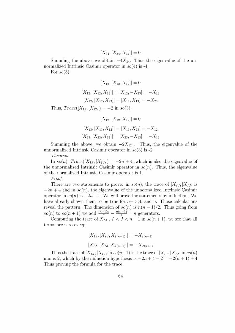
[X34, [X34, X34]] = 0

Summing the above, we obtain −4X34. Thus the eigenvalue of the un-normalized Intrinsic Casimir operator in so(4) is -4.

For so(3):

[X12, [X12, X12]] = 0

[X12, [X12, X13]] = [X12,−X23] = −X13

[X12, [X12, X23]] = [X12, X13] = −X23

Thus, Trace([X12, [X12, ) = −2 in so(3).

[X12, [X12, X12]] = 0

[X13, [X13, X12]] = [X13, X23] = −X12

[X23, [X23, X12]] = [X23,−X13] = −X12

Summing the above, we obtain −2X12 . Thus, the eigenvalue of theunnormalized Intrinsic Casimir operator in so(3) is -2.

TheoremIn so(n), Trace([XIJ , [XIJ , ) = −2n + 4 ,which is also the eigenvalue of

the unnormalized Intrinsic Casimir operator in so(n). Thus, the eigenvalueof the normalized Intrinsic Casimir operator is 1.

Proof:There are two statements to prove: in so(n), the trace of [XIJ , [XIJ , is

−2n + 4 and in so(n), the eigenvalue of the unnormalized Intrinsic Casimiroperator in so(n) is −2n+4. We will prove the statements by induction. Wehave already shown them to be true for n= 3,4, and 5. Those calculationsreveal the pattern. The dimension of so(n) is n(n − 1)/2. Thus going from

so(n) to so(n + 1) we add (n+1)n2

− n(n−1)2

= n generators.Computing the trace of XIJ , I < J < n + 1 in so(n + 1), we see that all

terms are zero except

[XIJ , [XIJ , XI(n+1)]] = −XI(n+1)

[XIJ , [XIJ , XJ(n+1)]] = −XJ(n+1)

Thus the trace of [XIJ , [XIJ , in so(n+1) is the trace of [XIJ , [XIJ , in so(n)minus 2, which by the induction hypothesis is −2n + 4− 2 = −2(n + 1) + 4Thus proving the formula for the trace.

64

In the intrinsic Casimir operator, going from so(n) to so(n+1), there aren new terms and when acting on XIJ , they are all zero except:

[XI(n+1), [XI(n+1), XIJ ]] = −XIJ

[XJ(n+1), [XJ(n+1), XIJ ]] = −XIJ

Thus, the eigenvalue of the intrinsic Casimir operator is also decreased by2 and the same calculation shows the validity of the formula for the eigenvalueof the intrinsic Casimir operator.

Thus the normalized Intrinsic Casimir Operator of so(n), when acting onso(n), is not just a multiple of the identity, it is the identity operator.

The higher order intrinsic Casimir operators of so(n) follow the patternof so(3).

11 The intrinsic Casimir Operators of su(2)

and su(3)

The “so(3) basis” for su(2) is:

α1 =

(0 −i/2

−i/2 0

)

α2 =

(0 −1/2

1/2 0

)

α3 =

(−i/2 0

0 i/2

)and the commutation relations are:

[α1, α2] = α3

[α2, α3] = α1

[α3, α1] = α2

In this basis, the commutation relations are identical with those of so(3) andhence the intrinsic Casimir operators are the same:

C2A = [α1, [α1, A]] + [α2, [α2, A]] + [α3, [α3, A]] = −2A

65

Since su(2) is isomorphic to so(3), it also possesses third order intrinsicCasimir operators. The third order intrinsic Casimir operators of su(2) are:

C3−A = [α1, [α2, [α3, A]]] + [α3, [α1, [α2, A]]]

+[α2, [α3, [α1, A]]] = −A

C3+A = [α3, [α2, [α1, A]]] + [α1, [α3, [α2, A]]]

+[α2, [α1, [α3, A]]] = A

And we have the identity in su(2):

C3−A = C2A + C3

+A

The standard basis for su(2) is:

β1 =

(0 −i−i 0

)

β2 =

(0 −11 0

)

β3 =

(−i 00 i

)and the commutation relations are:[β1, β2] = 2β3, [β2, β3] = 2β1, [β3, β1] = 2β2

Since βi = 2αi, in this basis, the intrinsic Casimir operator is:

CA = [β1, [β1, A]] + [β2, [β2, A]] + [β3, [β3, A]] = −8A

The Lie Algebra u(3) consists of the matrices:

X1 =

0 0 00 0 −10 1 0

X2 =

0 0 10 0 0−1 0 0

66

X3 =

0 −1 01 0 00 0 0

Y1 =

0 0 00 0 i0 i 0

Y2 =

0 0 i0 0 0i 0 0

Y3 =

0 i 0i 0 00 0 0

D1 =

i 0 00 0 00 0 0

D2 =

0 0 00 i 00 0 0

D3 =

0 0 00 0 00 0 i

The intrinsic Casimir operator is a linear combination of the basis el-

ements applied twice. The diagonal elements acting on diagonal elementsmust yield zero. Thus the non-diagonal elements determine the eigenvalueof the intrinsic Casimir operator acting on diagonal elements. Thus, in orderto determine the eigenvalue of the intrinsic Casimir Operator for u(3), allwe need to do is to calculate the action of the non-diagonal elements on thediagonal elements. The action of the diagonal elements is given by:

[D1, X1] = 0

[D2, X1] = −Y1

67

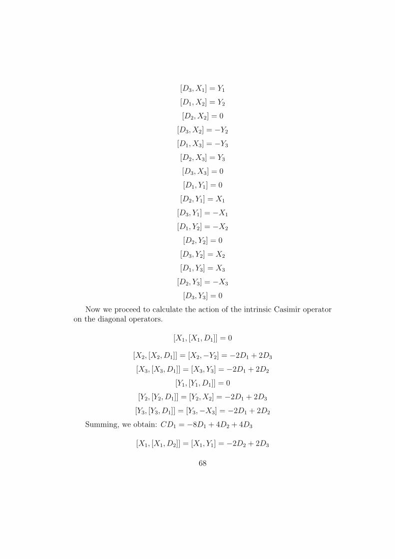
[D3, X1] = Y1

[D1, X2] = Y2

[D2, X2] = 0

[D3, X2] = −Y2

[D1, X3] = −Y3

[D2, X3] = Y3

[D3, X3] = 0

[D1, Y1] = 0

[D2, Y1] = X1

[D3, Y1] = −X1

[D1, Y2] = −X2

[D2, Y2] = 0

[D3, Y2] = X2

[D1, Y3] = X3

[D2, Y3] = −X3

[D3, Y3] = 0

Now we proceed to calculate the action of the intrinsic Casimir operatoron the diagonal operators.

[X1, [X1, D1]] = 0

[X2, [X2, D1]] = [X2,−Y2] = −2D1 + 2D3

[X3, [X3, D1]] = [X3, Y3] = −2D1 + 2D2

[Y1, [Y1, D1]] = 0

[Y2, [Y2, D1]] = [Y2, X2] = −2D1 + 2D3

[Y3, [Y3, D1]] = [Y3,−X3] = −2D1 + 2D2

Summing, we obtain: CD1 = −8D1 + 4D2 + 4D3

[X1, [X1, D2]] = [X1, Y1] = −2D2 + 2D3

68

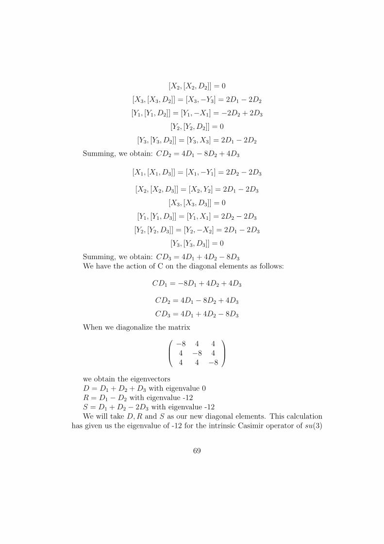
[X2, [X2, D2]] = 0

[X3, [X3, D2]] = [X3,−Y3] = 2D1 − 2D2

[Y1, [Y1, D2]] = [Y1,−X1] = −2D2 + 2D3

[Y2, [Y2, D2]] = 0

[Y3, [Y3, D2]] = [Y3, X3] = 2D1 − 2D2

Summing, we obtain: CD2 = 4D1 − 8D2 + 4D3

[X1, [X1, D3]] = [X1,−Y1] = 2D2 − 2D3

[X2, [X2, D3]] = [X2, Y2] = 2D1 − 2D3

[X3, [X3, D3]] = 0

[Y1, [Y1, D3]] = [Y1, X1] = 2D2 − 2D3

[Y2, [Y2, D3]] = [Y2,−X2] = 2D1 − 2D3

[Y3, [Y3, D3]] = 0

Summing, we obtain: CD3 = 4D1 + 4D2 − 8D3

We have the action of C on the diagonal elements as follows:

CD1 = −8D1 + 4D2 + 4D3

CD2 = 4D1 − 8D2 + 4D3

CD3 = 4D1 + 4D2 − 8D3

When we diagonalize the matrix −8 4 44 −8 44 4 −8

we obtain the eigenvectorsD = D1 + D2 + D3 with eigenvalue 0R = D1 −D2 with eigenvalue -12S = D1 + D2 − 2D3 with eigenvalue -12We will take D, R and S as our new diagonal elements. This calculation

has given us the eigenvalue of -12 for the intrinsic Casimir operator of su(3)

69

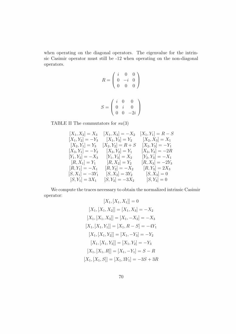
when operating on the diagonal operators. The eigenvalue for the intrin-sic Casimir operator must still be -12 when operating on the non-diagonaloperators.

R =

i 0 00 −i 00 0 0

S =

i 0 00 i 00 0 −2i

TABLE II The commutators for su(3)

[X1, X2] = X3 [X1, X3] = −X2 [X1, Y1] = R− S[X1, Y2] = −Y3 [X1, Y3] = Y2 [X2, X3] = X1

[X2, Y1] = Y3 [X2, Y2] = R + S [X2, Y3] = −Y1

[X3, Y1] = −Y2 [X3, Y2] = Y1 [X3, Y3] = −2R[Y1, Y2] = −X3 [Y1, Y3] = X2 [Y2, Y3] = −X1

[R,X1] = Y1 [R,X2] = Y2 [R,X3] = −2Y3

[R, Y1] = −X1 [R, Y2] = −X2 [R, Y3] = 2X3

[S, X1] = −3Y1 [S, X2] = 3Y2 [S, X3] = 0[S, Y1] = 3X1 [S, Y2] = −3X2 [S, Y3] = 0

We compute the traces necessary to obtain the normalized intrinsic Casimiroperator:

[X1, [X1, X1]] = 0

[X1, [X1, X2]] = [X1, X3] = −X2

[X1, [X1, X3]] = [X1,−X2] = −X3

[X1, [X1, Y1]] = [X1, R− S] = −4Y1

[X1, [X1, Y2]] = [X1,−Y3] = −Y2

[X1, [X1, Y3]] = [X1, Y2] = −Y3

[X1, [X1, R]] = [X1,−Y1] = S −R

[X1, [X1, S]] = [X1, 3Y1] = −3S + 3R

70

Then the trace of [X1, [X1, is -12. In the same manner, the trace of[X2, [X2, and [X3, [X3, are shown to be -12.

[Y1, [Y1, X1]] = [Y1, S −R] = −4X1

[Y1, [Y1, X2]] = [Y1,−Y3] = −X2

[Y1, [Y1, X3]] = [Y1, Y2] = −X3

[Y1, [Y1, Y1]] = 0

[Y1, [Y1, Y2]] = [Y1,−X3] = −Y2

[Y1, [Y1, Y3]] = [Y1, X2] = −Y3

[Y1, [Y1, R]] = [Y1, X1] = S −R

[Y1, [Y1, S]] = [Y1,−3X1] = −3S + 3R

Thus, the trace of [Y1, [Y1, is -12.In the same manner, the traces of [Y2, [Y2, and [Y3, [Y3, are shown to be

-12.

[R, [R,X1]] = [R, Y1] = −X1

[R, [R,X2]] = [R, Y2] = −X2

[R, [R,X3]] = [R,−2Y3] = −4X3

[R, [R, Y1]] = [R,−X1] = −Y1

[R, [R, Y2]] = [R,−X2] = −Y2

[R, [R, Y3]] = [R, 2X3] = −4Y3

[R, [R,R]] = 0

[R, [R,S]] = 0

Thus, the trace of [R, [R, is -12.

[S, [S, X1]] = [S,−3Y1] = −9X1

[S, [S, X2]] = [S, 3Y2] = −9X2

[S, [S, X3]] = 0

[S, [S, Y1]] = [S, 3X1] = −9Y1

71

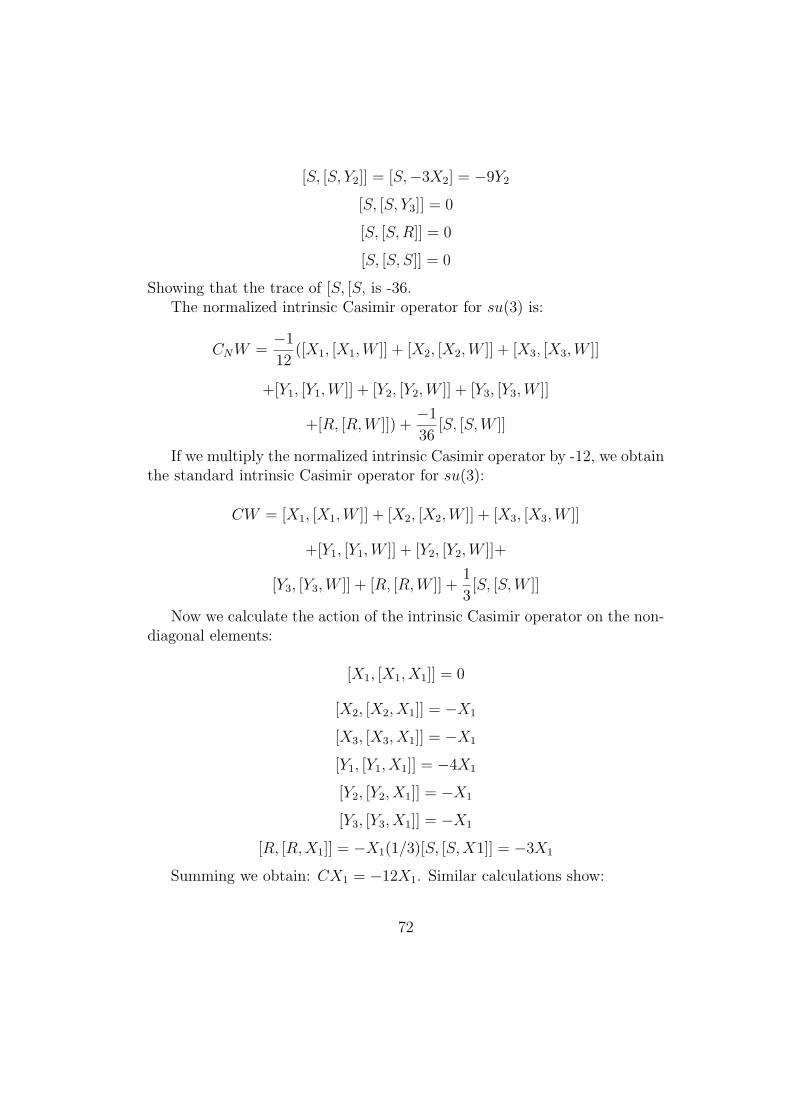
[S, [S, Y2]] = [S,−3X2] = −9Y2

[S, [S, Y3]] = 0

[S, [S, R]] = 0

[S, [S, S]] = 0

Showing that the trace of [S, [S, is -36.The normalized intrinsic Casimir operator for su(3) is:

CNW =−1

12([X1, [X1, W ]] + [X2, [X2, W ]] + [X3, [X3, W ]]

+[Y1, [Y1, W ]] + [Y2, [Y2, W ]] + [Y3, [Y3, W ]]

+[R, [R,W ]]) +−1

36[S, [S, W ]]

If we multiply the normalized intrinsic Casimir operator by -12, we obtainthe standard intrinsic Casimir operator for su(3):

CW = [X1, [X1, W ]] + [X2, [X2, W ]] + [X3, [X3, W ]]

+[Y1, [Y1, W ]] + [Y2, [Y2, W ]]+

[Y3, [Y3, W ]] + [R, [R,W ]] +1

3[S, [S, W ]]

Now we calculate the action of the intrinsic Casimir operator on the non-diagonal elements:

[X1, [X1, X1]] = 0

[X2, [X2, X1]] = −X1

[X3, [X3, X1]] = −X1

[Y1, [Y1, X1]] = −4X1

[Y2, [Y2, X1]] = −X1

[Y3, [Y3, X1]] = −X1

[R, [R,X1]] = −X1(1/3)[S, [S, X1]] = −3X1

Summing we obtain: CX1 = −12X1. Similar calculations show:

72

CX2 = −12X2

CX3 = −12X3

CY1 = −12Y1

CY2 = −12Y2

CY3 = −12Y3

CR = −12R

CS = −12S

Thus the eigenvalue of the standard intrinsic Casimir operator of su(3)is -12 and the eigenvalue of the normalized intrinsic Casimir operator is 1.

12 The Casimir Operator of su(n)

As with so(n), let eIJ denote the n by n matrix with 1 in the IJ positionand zero elsewhere. A basis for u(n) consists of the matrices

XIJ = eIJ − eJI

YIJ = i(eIJ + eJI)

DI = ieII

I < J, with the Lie brackets:

[XIJ , XKL] = δJKXIL + δJLXKI + δIKXLJ + δILXJK

[XIJ , YKL] = δJKYIL + δJLYKI − δIKYLJ − δILYJK

[YIJ , YKL] = −δJKXIL − δJLXKI − δIKXLJ − δILXJK

[XIJ , YIJ ] = DI −DJ

[DI , XIJ ] = YIJ

[DJ , XIJ ] = −YIJ

[DI , YIJ ] = −XIJ

[DJ , YIJ ] = XIJ

73

We first need to compute the trace of the elements of the Lie algebra. Westart with the trace of X12 in su(5) as a representative calculation:

[X12, [X12, X12]] = 0

[X12, [X12, X13]] = [X12,−X23] = −X13

[X12, [X12, X14]] = [X12,−X24] = −X14

[X12, [X12, X15]] = [X12,−X25] = −X15

[X12, [X12, X23]] = [X12, X13] = −X23

[X12, [X12, X24]] = [X12, X14] = −X24

[X12, [X12, X25]] = [X12, X15] = −X25

[X12, [X12, X34]] = 0

[X12, [X12, X35]] = 0

[X12, [X12, X45]] = 0

[X12, [X12, Y12]] = −4Y12

[X12, [X12, Y13]] = [X12,−Y23] = −Y13

[X12, [X12, Y14]] = [X12,−Y24] = −Y14

[X12, [X12, Y15]] = [X12,−Y25] = −Y15

[X12, [X12, Y23]] = [X12, Y13] = −Y23

[X12, [X12, Y24]] = [X12, Y14] = −Y24

[X12, [X12, Y25]] = [X12, Y15] = −Y25

[X12, [X12, Y34]] = 0

[X12, [X12, Y35]] = 0

[X12, [X12, Y45]] = 0

Trace of [X12, [X12, = −20 in su(5).We proceed with the terms of the Casimir operator of su(5):

[X12, [X12, X45]] = 0

74

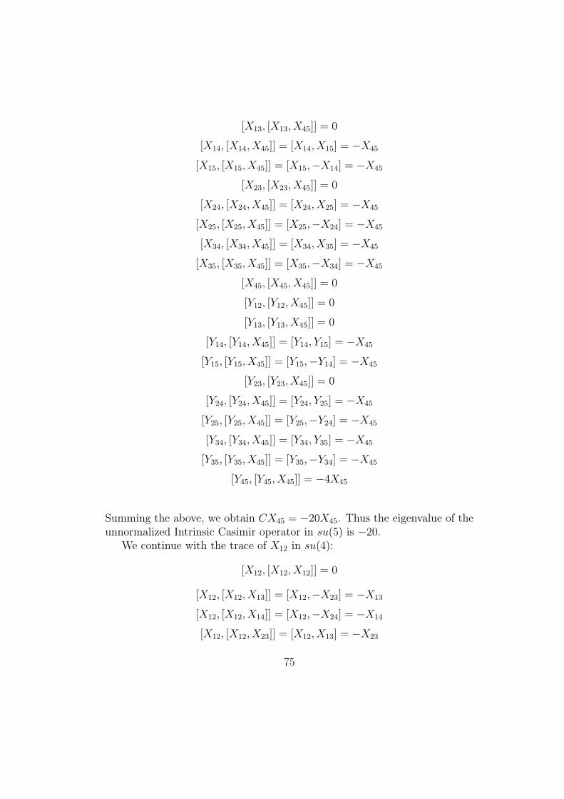
[X13, [X13, X45]] = 0

[X14, [X14, X45]] = [X14, X15] = −X45

[X15, [X15, X45]] = [X15,−X14] = −X45

[X23, [X23, X45]] = 0

[X24, [X24, X45]] = [X24, X25] = −X45

[X25, [X25, X45]] = [X25,−X24] = −X45

[X34, [X34, X45]] = [X34, X35] = −X45

[X35, [X35, X45]] = [X35,−X34] = −X45

[X45, [X45, X45]] = 0

[Y12, [Y12, X45]] = 0

[Y13, [Y13, X45]] = 0

[Y14, [Y14, X45]] = [Y14, Y15] = −X45

[Y15, [Y15, X45]] = [Y15,−Y14] = −X45

[Y23, [Y23, X45]] = 0

[Y24, [Y24, X45]] = [Y24, Y25] = −X45

[Y25, [Y25, X45]] = [Y25,−Y24] = −X45

[Y34, [Y34, X45]] = [Y34, Y35] = −X45

[Y35, [Y35, X45]] = [Y35,−Y34] = −X45

[Y45, [Y45, X45]] = −4X45

Summing the above, we obtain CX45 = −20X45. Thus the eigenvalue of theunnormalized Intrinsic Casimir operator in su(5) is −20.

We continue with the trace of X12 in su(4):

[X12, [X12, X12]] = 0

[X12, [X12, X13]] = [X12,−X23] = −X13

[X12, [X12, X14]] = [X12,−X24] = −X14

[X12, [X12, X23]] = [X12, X13] = −X23

75

[X12, [X12, X24]] = [X12, X14] = −X24

[X12, [X12, X34]] = 0

[X12, [X12, Y12]] = −4Y12

[X12, [X12, Y13]] = [X12,−Y23] = −Y13

[X12, [X12, Y14]] = [X12,−Y24] = −Y14

[X12, [X12, Y23]] = [X12, Y13] = −Y23

[X12, [X12, Y24]] = [X12, Y14] = −Y24

[X12, [X12, Y34]] = 0

Trace of [X12, [X12, = −16 in su(4).We proceed with the terms of the Casimir operator of su(4):

[X12, [X12, X34]] = 0

[X13, [X13, X34]] = [X13, X14] = −X34

[X14, [X14, X34]] = [X14,−X13] = −X34

[X23, [X23, X34]] = [X23, X24] = −X34

[X24, [X24, X34]] = [X24,−X23] = −X34

[X34, [X34, X34]] = 0

[Y12, [Y12, X34]] = 0

[Y13, [Y13, X34]] = [Y13, X14] = −X34

[Y14, [Y14, X34]] = [Y14,−X13] = −X34

[Y23, [Y23, X34]] = [Y23, X24] = −X34

[Y24, [Y24, X34]] = [Y24,−X23] = −X34

[Y34, [Y34, X34]] = −4X34

Summing the above, we obtain CX34 = −16X34. Thus the eigenvalue of theunnormalized Intrinsic Casimir operator in su(4) is −16.

We continue with the trace of X12 in su(3):

[X12, [X12, X12]] = 0

76

[X12, [X12, X13]] = [X12,−X23] = −X13

[X12, [X12, X23]] = [X12, X13] = −X23

[X12, [X12, Y12]] = −4Y12

[X12, [X12, Y13]] = [X12,−X23] = −X13

[X12, [X12, Y23]] = [X12, Y13] = −X23

Trace of [X12, [X12, = −12 in su(3).We proceed with the terms of the Casimir operator of su(3):

[X12, [X12, X12]] = 0

[X13, [X13, X12]] = [X13, X23] = −X12

[X23, [X23, X12]] = [X23,−X13] = −X12

[Y12, [Y12, X12]] = 0

[Y13, [Y13, X12]] = [Y13, Y23] = −X12

[Y23, [Y23, X12]] = [Y23,−Y13] = −X12

Summing the above, we obtain CX34 = −12X34. Thus, the eigenvalue ofthe unnormalized Intrinsic Casimir operator in su(3) is −12.

Theorem In su(n), the trace of [XIJ , [XIJ , is −4n which is also the eigen-value of the unnormalized Intrinsic Casimir operator in su(n). Thus, theeigenvalue of the normalized Intrinsic Casimir operator is 1.

Proof There are two statements to prove: in su(n), the trace of [XIJ , [XIJ ,is −4n and in su(n), the eigenvalue of the unnormalized Intrinsic Casimiroperator in su(n) is −4n. We will prove the statements by induction. Wehave already shown them to be true for n = 3, 4, and 5. Those calculationsreveal the patterns. The dimension of su(n) is n2−1. Thus going from su(n)to su(n + 1) we add (n + 1)2− 1− (n2− 1) = 2n + 1 generators. Computingthe trace of XIJ , I < J < n + 1. we see that all terms are zero except

[XIJ , [XIJ , XI(n+1)]] = −XI(n+1)

[XIJ , [XIJ , XJ(n+1)]] = −XJ(n+1)

[XIJ , [XIJ , YI(n+1)]] = −YI(n+1)

[XIJ , [XIJ , YJ(n+1)]] = −YJ(n+1)

77

Thus the trace of [XIJ , [XIJ , in su(n + 1) = the trace of [XIJ , [XIJ , insu(n) minus 4, which by the induction hypothesis is −4n − 4 = −4(n + 1)Thus proving the formula for the trace.

In the intrinsic Casimir operator, there are n new terms and when actingon XIJ , they are all zero except:

[XI(n+1), [XI(n+1), XIJ ]] = −XIJ

[XJ(n+1), [XJ(n+1), XIJ ]] = −XIJ

[YI(n+1), [YI(n+1), XIJ ]] = −XIJ

[YJ(n+1), [YJ(n+1), XIJ ]] = −XIJ

Thus, the eigenvalue of the intrinsic Casimir operator is also decreased by4 and the same calculation show the validity of the formula for the eigenvalueof the intrinsic Casimir operator. Thus the normalized Intrinsic intrinsicCasimir Operator of su(n) is not just a multiple of the identity, it is theidentity operator, but only when acting on elements of su(n)!

13 An Attempt at Reconciliation

Perhaps we can reconcile the two different ways of looking at the Casimiroperator if we expand the action of the intrinsic Casimir operator of so(3) interms of matrix multiplication:

CA = [X1, [X1, A]] + [X2, [X2, A]] + [X3, [X3, A]] (27)

= [X1, X1A− AX1] + [X2, X2A− AX2]] + [X3, X3A−X3]

= X1X1A−X1AX1 + X2X2A−X2AX2 + X3X3A−X3AX3

−(X1AX1 − AX1X1 + X2AX2 − AX2X2 + X3AX3 − AX3X3)

= X1X1A + X2X2A + X3X3A− 2X1AX1 − 2X2AX2 − 2X3AX3

+AX1X1 + AX2X2 + AX3X3

= (X1X1 + X2X2 + X3X3)A− 2X1AX1 − 2X2AX2 − 2X3AX3

+A(X1X1 + X2X2 + X3X3)

78

= (X1X1 + X2X2 + X3X3)A (28)

(a)−2(X1AX1 + X2AX2 + X3AX3)

(b)+A(X1X1 + X2X2 + X3X3)

(c)The terms in (28) have been labeled in order to facilitate discussion. The

expressions in parentheses in (28) (a and c), i.e. the sum of the squares

(X1X1 + X2X2 + X3X3)

is the standard way of interpreting the intrinsic Casimir operator. Thus,the sum of the squares of the matrices is a multiple of the identity matrix,but this is not an invariant operator since the eigenvalue varies with therepresentation. The invariant operator is obtained as the sum of the matrixterms and its eigenvalue does not depend on the representation.

There is another point of confusion in Quantum Mechanics: the dual roleof the Casimir operator as a matrix operator and as an invariant differentialoperator. Acting on elements of the Lie algebra the intrinsic Casimir operatorhas only one eigenvalue. Acting on functions, the intrinsic Casimir opera-tor has an infinite range of eigenvalues. Schiff [26](p. 82) has the Casimiroperator (as differential operator) acting on the spherical harmonics:

L2Ylm(θ, φ) = l(l + 1)Ylm(θ, φ)

This action of L2 is as a differential operator acting on functions definedon the manifold SO(3). Because Schiff follows the physics tradition andmultiplies each generator by a factor of i in our notation we would haveinstead:

CYlm(θ, φ) = −l(l + 1)Ylm(θ, φ)

The standard approach to quantum theory of angular momentum at-tempts to force the matrix representations do the job the eigenfunctionsshould be doing.

In order to obtain a spectrum from the Casimir operator using matrices,the standard approach requires an new representation. In order to obtain a

79

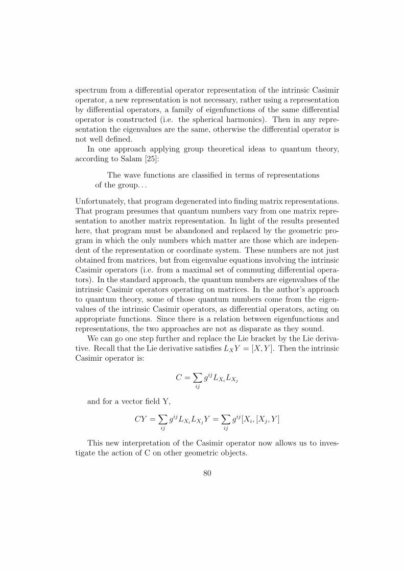
spectrum from a differential operator representation of the intrinsic Casimiroperator, a new representation is not necessary, rather using a representationby differential operators, a family of eigenfunctions of the same differentialoperator is constructed (i.e. the spherical harmonics). Then in any repre-sentation the eigenvalues are the same, otherwise the differential operator isnot well defined.

In one approach applying group theoretical ideas to quantum theory,according to Salam [25]:

The wave functions are classified in terms of representationsof the group. . .

Unfortunately, that program degenerated into finding matrix representations.That program presumes that quantum numbers vary from one matrix repre-sentation to another matrix representation. In light of the results presentedhere, that program must be abandoned and replaced by the geometric pro-gram in which the only numbers which matter are those which are indepen-dent of the representation or coordinate system. These numbers are not justobtained from matrices, but from eigenvalue equations involving the intrinsicCasimir operators (i.e. from a maximal set of commuting differential opera-tors). In the standard approach, the quantum numbers are eigenvalues of theintrinsic Casimir operators operating on matrices. In the author’s approachto quantum theory, some of those quantum numbers come from the eigen-values of the intrinsic Casimir operators, as differential operators, acting onappropriate functions. Since there is a relation between eigenfunctions andrepresentations, the two approaches are not as disparate as they sound.

We can go one step further and replace the Lie bracket by the Lie deriva-tive. Recall that the Lie derivative satisfies LXY = [X, Y ]. Then the intrinsicCasimir operator is:

C =∑ij

gijLXiLXj

and for a vector field Y,

CY =∑ij

gijLXiLXj

Y =∑ij

gij[Xi, [Xj, Y ]

This new interpretation of the Casimir operator now allows us to inves-tigate the action of C on other geometric objects.

80

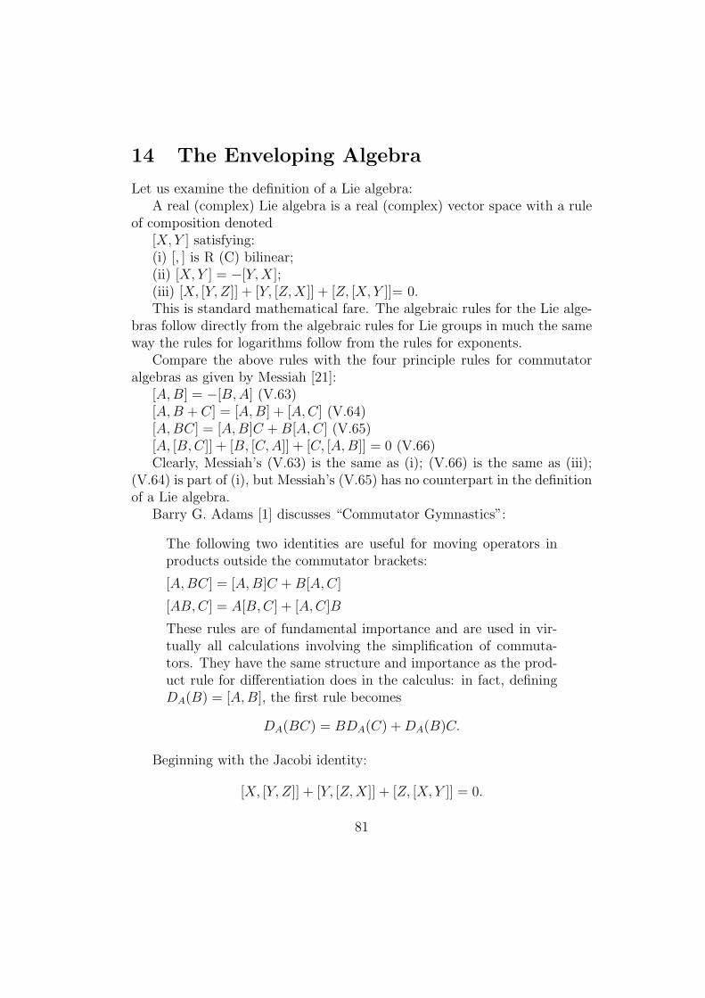
14 The Enveloping Algebra

Let us examine the definition of a Lie algebra:A real (complex) Lie algebra is a real (complex) vector space with a rule

of composition denoted[X, Y ] satisfying:(i) [, ] is R (C) bilinear;(ii) [X, Y ] = −[Y,X];(iii) [X, [Y, Z]] + [Y, [Z,X]] + [Z, [X, Y ]]= 0.This is standard mathematical fare. The algebraic rules for the Lie alge-

bras follow directly from the algebraic rules for Lie groups in much the sameway the rules for logarithms follow from the rules for exponents.

Compare the above rules with the four principle rules for commutatoralgebras as given by Messiah [21]:

[A, B] = −[B, A] (V.63)[A, B + C] = [A, B] + [A, C] (V.64)[A, BC] = [A, B]C + B[A, C] (V.65)[A, [B, C]] + [B, [C, A]] + [C, [A, B]] = 0 (V.66)Clearly, Messiah’s (V.63) is the same as (i); (V.66) is the same as (iii);

(V.64) is part of (i), but Messiah’s (V.65) has no counterpart in the definitionof a Lie algebra.

Barry G. Adams [1] discusses “Commutator Gymnastics”:

The following two identities are useful for moving operators inproducts outside the commutator brackets:

[A, BC] = [A, B]C + B[A, C]

[AB, C] = A[B, C] + [A, C]B

These rules are of fundamental importance and are used in vir-tually all calculations involving the simplification of commuta-tors. They have the same structure and importance as the prod-uct rule for differentiation does in the calculus: in fact, definingDA(B) = [A, B], the first rule becomes

DA(BC) = BDA(C) + DA(B)C.

Beginning with the Jacobi identity:

[X, [Y, Z]] + [Y, [Z,X]] + [Z, [X, Y ]] = 0.

81

Take two terms to the right hand side of the equation:

[X, [Y, Z]] = −[Y, [Z,X]]− [Z, [X, Y ]]

Apply the anti-symmetry property to the two terms on the right handside:

(iv) [X, [Y, Z]] = [Y, [X, Z]] + [[X,Y ], Z]Comparing (iv) to the second of Adams’ relations and Messiah’s (v.65)

we see a structural similarity. And, indeed, if we define DX(Y ) = [X, Y ]then we have the identity:

DX([Y, Z]) = [Y,DX(Z)] + [DX(Y ), Z].

This derivative is well known and is called the Lie derivative.Thus it seems that the derivative defined by Adams is a cheap parody, a

grotesque caricature of the Lie derivative.The rules of “commutator gymnastics” are not the rules for Lie algebras

and chaos follows if the two are confused.Revisit the definition: a Lie algebra is a vector space equipped with an

operation denoted by [A, B]. There is no mention of the Lie algebra beingequipped with a product AB. Indeed, it is not part of the definition. Oncetwo matrices are multiplied together, the product is outside the structure ofLie Algebras.

Let us digress and discuss a more elementary example. The allowedoperations on a logarithm are:

log(xy) = logx + logy

log(x/y) = logx− logy

logyr = rlogy

Now, logx and logy are real numbers and real numbers can be multipliedtogether: (logx)(logy). But the product has no significance as a logarithm,unless you are changing bases.

The transition from Lie Algebra to Lie Group is via the exponential map.Thus the map from Lie Group to Lie Algebra is the logarithm. In this case,we are dealing with matrices, and matrices (even those which represent Liealgebras) can be multiplied together, but once you have multiplied them to-gether, they have ceased to have significance as logarithms, they have ceased

82

to represent the Lie algebra. Multiplication of matrices is meaningless in thecontext of Lie algebras (except as a tool for computing the Lie bracket withina given representation).

For a Lie algebra L , the universal enveloping algebra of L , U(L) isthe “free algebra” with the elements of L as generators modulo the relationXY − Y X − [X, Y ] = 0 [9] (pp. 72-73).

Alternately, [5] the universal enveloping algebra of L can be defined interms of the tensor algebra of L which is a vector space over the field k. Ifwe define

Tn = L ⊗ L⊗ L . . .⊗ L

(n factors of L ), with T0 = kDefine

T = T0 ⊗ T1 ⊗ T2 ⊗ . . . Tn ⊗ . . .

The product in T is just tensor multiplication.Let J be the two-sided ideal of T generated by all objects

X ⊗ Y − Y ⊗X − [X,Y ]

for all X,Y in L . In this setting, U(L) = T/J . The two definitions areequivalent but the second is more elegant.

In the enveloping algebra approach, the Casimir operators are the ele-ments of the center of U(L), which is denoted Z(L). If we are to keep thisrelationship with our reinterpretation of the Casimir operator, we must alsoreinterpret the universal enveloping algebra formalism.

The relation X ⊗ Y − Y ⊗X − [X, Y ] = 0 holds in U(L) and is supposedto mimic the relation XY −Y X = [X,Y ], which as Hermann [9] points out isan attempt to force a meaning to the symbol XY. If this is the case, exactlywhat meaning does the theory of the enveloping algebra force upon XY? Thesymbol XY can be given a meaning without such elaborate underpinnings.As we did with the intrinsic Casimir operator, we can interpret XY as anoperator: XY Z becomes [X, [Y, Z]]. To emphasize this interpretation, wewill write [X,[Y instead of just XY.

From the Jacobi identity, for X, Y, Z ∈ L,

[X, [Y, Z]]− [Y, [X, Z]] = [[X, Y ], Z]

Dropping the Z], we obtain an operator equation:

83

[X, [Y,−[Y, [X, = [[X, Y ],

With this interpretation, the relation X ⊗ Y − Y ⊗ X − [X, Y ] in thedefinition of U(L) is shown to be the Jacobi identity, not the commutator (orperhaps we should say that the commutator and the Jacobi identity are thesame). Geometrically, we are replacing the element X of the Lie algebra bythe Lie derivative with respect to X. The Lie derivative satisfies:

LXLY − LYLX = L[X,Y ]

Indeed, since LXZ = [X, Z], the rearranged Jacobi identity:

[X, [Y, Z]]− [Y, [X, Z]] = [[X, Y ], Z]

is a Lie derivative equation:

LXLY (Z)− LYLX(Z) = L[X,Y ]Z

So it seems that we are led to interpret the universal enveloping algebraof L , U(L) as the “free algebra” with generators the Lie derivatives withrespect to the elements of L . The equivalence relation “modulo the relationXY − Y X − [X, Y ]” is not necessary since it is built into the Lie derivative.

To avoid confusion, we need a name for the new formalism and I suggestit be called the “geometric enveloping algebra.”

In the Enveloping algebra approach to the Casimir operator, the Casimiroperator is taken to be an element of the Enveloping Algebra in which caseC2Y =

∑ij gijXi ⊗Xj ⊗ Y , with the tensor product as the multiplication.

In the geometric enveloping algebra, this translates as:

CY =∑ij

gij[Xi, [Xj, [Y (29)

This provides an alternative way of interpreting the symbols, but it isnot a definition of the Casimir operator C, instead, (29) is a definition of theoperator CY . Still, some expressions in the standard theory of envelopingalgebras must be interpreted in terms of (29) instead of (8). The differencebetween (29) and (8) comes down to the difference in roles of X and Y in theexpression [X, Y ] interpreted as the operator, [X, acting on the element of

84

the vector space, Y ]. This is the same problem in mathematical semanticsaddressed by Dirac in his treatment of Bras and Kets. If Y is being actedupon (a ket), then (8) holds and is viewed as

C2(Y ]) =∑ij

gij[Xi, [Xj, Y ]] (30)

If instead, Y is viewed as an operator (a bra), then (29) holds and isviewed as:

C([Y ) =∑ij

gij[Xi, [Xj, [Y, (31)

The geometric enveloping algebra is associative because left bracketingis a function from L to L and composition of functions is associative. Theenveloping algebra has only bras, no kets. Thus, we could say that the LieBracket is “left associative” and becomes non-associative only when left andright brackets are mixed. A free algebra of only kets would also be associative.The Lie bracket is also right associative. It is only when bras and kets aremixed that the algebra becomes nonassociative.

15 Intrinsic Casimir operators with eigenvalue

Zero

Examining the commutators for so(3, 1), we observe that there are preciselytwo ways to obtain each XI :

[X2, X3] = X1

[N2, N3] = −X1

[X3, X1] = X2

[N3, N1] = −X2

[X1, X2] = X3

[N1, N2] = −X3

Thus we can write the Zero operator as:

0 = X1 −X1 + X2 −X2 + X3 −X3

85

= [X2, X3] + [N2, N3] + [X3, X1] + [N3, N1] + [X1, X2] + [N1, N2]

Which arises in the expansion of

σ2Y = [X1, [X2, Y ]] + [X2, [X3, Y ]] + [X3, [X1, Y ]]

+[N1, [N2, Y ]] + [N2, [N3, Y ]] + [N3, [N1, Y ]]

and we check the eigenvalues:

σ2X1 = [X1, [X2, X1]] + [X2, [X3, X1]] + [X3, [X1, X1]]

+[N1, [N2, X1]] + [N2, [N3, X1]] + [N3, [N1, X1]]

= [X1,−X3] + [N1,−N3] = X2 −X2 = 0

σ2X2 = [X1, [X2, X2]] + [X2, [X3, X2]] + [X3, [X1, X2]]

+[N1, [N2, X2]] + [N2, [N3, X2]] + [N3, [N1, X2]]

= [X2,−X1] + [N2,−N1] = X3 −X3 = 0

σ2X3 = [X1, [X2, X3]] + [X2, [X3, X3]] + [X3, [X1, X3]]

+[N1, [N2, X3]] + [N2, [N3, X3]] + [N3, [N1, X3]]

= [X3,−X2] + [N3,−N2] = X1 −X1 = 0

σ2N1 = [X1, [X2, N1]] + [X2, [X3, N1]] + [X3, [X1, N1]]

+[N1, [N2, N1]] + [N2, [N3, N1]] + [N3, [N1, N1]]

= [X1,−N3] + [N1, X3] = N2 −N2 = 0

σ2N2 = [X1, [X2, N2]] + [X2, [X3, N2]] + [X3, [X1, N2]]

+[N1, [N2, N2]] + [N2, [N3, N2]] + [N3, [N1, N2]]

= [X2,−N1] + [N2, X1] = N3 −N3 = 0

σ2N3 = [X1, [X2, N3]] + [X2, [X3, N3]] + [X3, [X1, N3]]

+[N1, [N2, N3]] + [N2, [N3, N3]] + [N3, [N1, N3]]

86

= [X3,−N2] + [N3, X2] = −N1 + N1 = 0

Thus σ2 is a Casimir operator with eigenvalue zero.We can repeat the process by noting that there are two ways to obtain

each NI .Starting with the relations:

[X2, N3] = N1

−[N2, X3] = −N1

[X3, N1] = N2

−[N3, X1] = −N2

[X1, N2] = N3

−[N1, X2] = −N3

we add to obtain:

[X2, N3]− [N2, X3] + [X3, N1]− [N3, X1] + [X1, N2]− [N1, X2] = 0

Which arises in the expansion of:

κY = [X2, [N3, Y ]]− [N2, [X3, Y ]] + [X3, [N1, Y ]]

−[N3, [X1, Y ]] + [X1, [N2, Y ]]− [N1, [X2, Y ]]

Computing the action of κ, we obtain:

κX1 = [X2, [N3, X1]]− [N2, [X3, X1]] + [X3, [N1, X1]]

−[N3, [X1, X1]] + [X1, [N2, X1]]− [N1, [X2, X1]]

= [X1,−N3]− [N1, X3] = N2 −N2 = 0

κX2 = [X2, [N3, X2]]− [N2, [X3, X2]] + [X3, [N1, X2]]

−[N3, [X1, X2]] + [X1, [N2, X2]]− [N1, [X2, X2]]

= [X2,−N1]− [N2,−X1] = N3 −N3 = 0

κX3 = [X2, [N3, X3]]− [N2, [X3, X3]] + [X3, [N1, X3]]

87

−[N3, [X1, X3]] + [X1, [N2, X3]]− [N1, [X2, X3]]

= [X3,−N2]− [N3,−X2] = N1 −N1 = 0

κN1 = [X2, [N3, N1]]− [N2, [X3, N1]] + [X3, [N1, N1]]

−[N3, [X1, N1]] + [X1, [N2, N1]]− [N1, [X2, N1]]

= [X1, X3]− [N1,−N3] = −X2 + X2 = 0

κN2 = [X2, [N3, N2]]− [N2, [X3, N2]] + [X3, [N1, N2]]

−[N3, [X1, N2]] + [X1, [N2, N2]]− [N1, [X2, N2]]

= [X2, X1]− [N2,−N1] = −X3 + X3 = 0

κN3 = [X2, [N3, N3]]− [N2, [X3, N3]] + [X3, [N1, N3]]

−[N3, [X1, N3]] + [X1, [N2, N3]]− [N1, [X2, N3]]

= [X3, X2]− [N3,−N2] = −X1 + X1 = 0

Thus we have another unexpected Casimir operator of eigenvalue type.The Casimir operator

σ2Y = [X1, [X2, Y ]] + [X2, [X3, Y ]] + [X3, [X1, Y ]]

+[N1, [N2, Y ]] + [N2, [N3, Y ]] + [N3, [N1, Y ]]

may be viewed as being associated with the decomposition of so(3, 1) intothe so(3) subalgebra generated by the XI , and its complement, consistingof the NI . The corresponding operator with respect to the subalgebra 2decomposition is:

σ22Y = [X1, [N2, Y ]] + [N2, [N3, Y ]] + [N3, [X1, Y ]]

−[N1, [X2, Y ]] + [X2, [X3, Y ]]− [X3, [N1, Y ]]

We calculate:

σ22X1 = [X1, [N2, X1]] + [N2, [N3, X1]] + [N3, [X1, X1]]

−[N1, [X2, X1]] + [X2, [X3, X1]]− [X3, [N1, X1]]

88

= [X1,−N3]− [N1,−X3] = N2 −N2 = 0

σ22X2 = [X1, [N2, X2]] + [N2, [N3, X2]] + [N3, [X1, X2]]

−[N1, [X2, X2]] + [X2, [X3, X2]]− [X3, [N1, X2]]

= [N2,−N1] + [X2,−X1] = −X3 + X3 = 0

σ22X3 = [X1, [N2, X3]] + [N2, [N3, X3]] + [N3, [X1, X3]]

−[N1, [X2, X3]] + [X2, [X3, X3]]− [X3, [N1, X3]]

= [N3,−X2]− [X3,−N2] = N1 −N1 = 0

σ22N1 = [X1, [N2, N1]] + [N2, [N3, N1]] + [N3, [X1, N1]]

−[N1, [X2, N1]] + [X2, [X3, N1]]− [X3, [N1, N1]]

= [X1, X3]− [N1,−N3] = −X2 + X2 = 0

σ22N2 = [X1, [N2, N2]] + [N2, [N3, N2]] + [N3, [X1, N2]]

−[N1, [X2, N2]] + [X2, [X3, N2]]− [X3, [N1, N2]]

= [N2, X1] + [X2,−N1] = −N3 + N3 = 0

σ22N3 = [X1, [N2, N3]] + [N2, [N3, N3]] + [N3, [X1, N3]]

−[N1, [X2, N3]] + [X2, [X3, N3]]− [X3, [N1, N3]]

= [N3,−N2]− [X3, X2] = −X1 + X1 = 0

Thus σ22 is a Casimir operator with eigenvalue 0.

The operator constructed from subalgebra 3, corresponding to σ2 is:

σ23Y = [N1, [X2, Y ]] + [X2, [N3, Y ]] + [N3, [N1, Y ]]

−[X1, [N2, Y ]]− [N2, [X3, Y ]] + [X3, [X1, Y ]]

We calculate the action on a basis:

σ23X1 = [N1, [X2, X1]] + [X2, [N3, X1]] + [N3, [N1, X1]]

−[X1, [N2, X1]]− [N2, [X3, X1]] + [X3, [X1, X1]]

89

= [N1,−X3]− [X1,−N3] = N2 −N2 = 0

σ23X2 = [N1, [X2, X2]] + [X2, [N3, X2]] + [N3, [N1, X2]]

−[X1, [N2, X2]]− [N2, [X3, X2]] + [X3, [X1, X2]]

= [X2,−N1] + [N2,−X1] = N3 −N3 = 0

σ23X3 = [N1, [X2, X3]] + [X2, [N3, X3]] + [N3, [N1, X3]]

−[X1, [N2, X3]]− [N2, [X3, X3]] + [X3, [X1, X3]]

= [N3,−N2] + [X3,−X2]] = −X1 + X1 = 0

σ23N1 = [N1, [X2, N1]] + [X2, [N3, N1]] + [N3, [N1, N1]]

−[X1, [N2, N1]]− [N2, [X3, N1]] + [X3, [X1, N1]]

= [N1,−N3]− [X1, X3] = −X2 + X2 = 0

σ23N2 = [N1, [X2, N2]] + [X2, [N3, N2]] + [N3, [N1, N2]]

−[X1, [N2, N2]]− [N2, [X3, N2]] + [X3, [X1, N2]]

= [X2, X1]− [N2,−N1] = −X3 + X3 = 0

σ23N3 = [N1, [X2, N3]] + [X2, [N3, N3]] + [N3, [N1, N3]]

−[X1, [N2, N3]]− [N2, [X3, N3]] + [X3, [X1, N3]]

= [N3, X2] + [X3,−N2]] = −N1 + N1 = 0

This confirms that σ23 is a Casimir operator with eigenvalue 0.

The σ-like operator constructed for subalgebra 4 is:

σ24Y = [N1, [N2, Y ]] + [N2, [X3, Y ]] + [X3, [N1, Y ]]

+[X1, [X2, Y ]]− [X2, [N3, Y ]]− [N3, [X1, Y ]]

The calculations proceed as above:

σ24X1 = [N1, [N2, X1]] + [N2, [X3, X1]] + [X3, [N1, X1]]

+[X1, [X2, X1]]− [X2, [N3, X1]]− [N3, [X1, X1]]

90

= [N1,−N3] + [X1,−X3] = −X2 + X2 = 0

σ24X2 = [N1, [N2, X2]] + [N2, [X3, X2]] + [X3, [N1, X2]]

+[X1, [X2, X2]]− [X2, [N3, X2]]− [N3, [X1, X2]]

= [N2,−X1]− [X2,−N1] = N3 −N3 = 0

σ24X3 = [N1, [N2, X3]] + [N2, [X3, X3]] + [X3, [N1, X3]]

+[X1, [X2, X3]]− [X2, [N3, X3]]− [N3, [X1, X3]]

= [X3,−N2]− [N3,−X2] = N1 −N1 = 0

σ24N1 = [N1, [N2, N1]] + [N2, [X3, N1]] + [X3, [N1, N1]]

+[X1, [X2, N1]]− [X2, [N3, N1]]− [N3, [X1, N1]]

= [N1, X3] + [X1,−N3] = −N2 + N2 = 0

σ24N2 = [N1, [N2, N2]] + [N2, [X3, N2]] + [X3, [N1, N2]]

+[X1, [X2, N2]]− [X2, [N3, N2]]− [N3, [X1, N2]]

= [N2,−N1]− [X2, X1] = −X3 + X3 = 0

σ24N3 = [N1, [N2, N3]] + [N2, [X3, N3]] + [X3, [N1, N3]]

+[X1, [X2, N3]]− [X2, [N3, N3]]− [N3, [X1, N3]]

= [X3, X2]− [N3,−N2] = −X1 + X1 = 0

Thus σ24 is a Casimir operator with eigenvalue 0.

91

16 Solo Casimir Operators

Surprisingly, there is yet another type of intrinsic Casimir operator.The characteristic equation of the adjoint representation of X1 ∈ so(3) is

the determinant of

det

−λ 0 00 −λ −10 1 −λ

= −λ3 − λ

Since a matrix satisfies its own characteristic equation, we have:

−(adX1)3 − adX1 = 0

We use the property of the adjoint representation to write the operatorequation:

SX1 = [X1, [X1, [X1 + [X1 = 0

and we compute, for verification:

SX1X2 = [X1, [X1, [X1, X2]]] + [X1, X2]

= [X1, [X1, X3]] + X3 = [X1,−X2] + X3

= −X3 + X3 = 0

SX1X3 = [X1, [X1, [X1, X3]]] + [X1, X3] = 0

= [X1, [X1,−X2]]−X2

= [X1,−X3]−X2 = X2 −X2 = 0

Likewise, from the adjoint representation of X2 we obtain:

SX2 = [X2, [X2, [X2 + [X2 = 0

From the adjoint representation of X3 we obtain:

SX3 = [X3, [X3, [X3 + [X3 = 0

Thus, we have three more third order Casimir operators for so(3). Sincethe definition of SXi

involves only Xi, these are a novel sort of Casimiroperator which we will call solo-Casimir operators. We state the obvious:

92

Theorem on Solo-Casimir OperatorsEvery element of a simple Lie algebra L generates a solo Casimir operator.Proof: Let P (λ) be the characteristic equation of the matrix adX. Since

a matrix satisfies its own characteristic equation, we have: P (adX) = 0Thus, we have the operator equation P ([X) = 0 which defines a solo-Casimiroperator.

Observe that although the characteristic equation of adX has degree equalto the dimension of the Lie Algebra, there may be a polynomial of lowerdegree which adX may satisfy. The lowest degree polynomial which adXsatisfies will be called the degree of X.

We leave it to the interested reader to confirm that for a generic matrixM ,

SX1M = [X1, [X1, [X1, M ]]]+[X1, M ] =

0 0 00 3m23 + 3m32 −3m22 + 3m33

0 −3m22 + 3m33 −3m23 − 3m32

And furthermore, if a three by three matrix M is an eigenvector of all

three solo operators:

SX1M = [X1, [X1, [X1, M ]]] + [X1, M ] = 0

SX2M = [X2, [X2, [X2, M ]]] + [X2, M ] = 0

SX3M = [X3, [X3, [X3, M ]]] + [X3, M ] = 0

then M ∈ so(3).The su(2) solo operators follow the pattern for so(3):

S1 = [α1, [α1, [α1 + [α1

S2 = [α2, [α2, [α2 + [α2

S3 = [α3, [α3, [α3 + [α3

This construction of the third order solo-Casimir operators and the cal-culations done for so(3) needs to be done for so(2, 1). The characteristicequation for the matrix of Y1 in the adjoint representation is λ3 + λ = 0which leads us to consider the operator:

SY1 = [Y1, [Y1, [Y1 + [Y1

93

and we compute, for verification:

SY1Y2 = [Y1, [Y1, [Y1, Y2]]] + [Y1, Y2]

= [Y1, [Y1,−Y3]]− Y3

= [Y1,−Y2]− Y3 = Y3 − Y3 = 0

The other computations are left to the reader.Likewise, from the matrix of Y2 in the adjoint representation, we obtain

the characteristic equation λ3 − λ = 0 and hence, the operator:

SY2 = [Y2, [Y2, [Y2 − [Y2 = 0

and we compute, for verification:

SY2Y1 = [Y2, [Y2, [Y2, Y1]]]− [Y2, Y1]

= [Y2, [Y2, Y3]] + Y3

= [Y2, Y1]− Y3 = Y3 − Y3 = 0

Again, from the adjoint representation of Y3 we obtain:

SY3 = [Y3, [Y3, [Y3 − [Y3 = 0

We compute the action of the solo Casimir operator of so(3), SX1 , on theremaining elements of so(3, 1):

SX1N1 = [X1, [X1, [X1, N1]]] + [X1, N1] = 0

SX1N2 = [X1, [X1, [X1, N2]]] + [X1, N2]

= [X1, [X1, N3]] + N3

= [X1,−N2] + N3 = −N3 + N3 = 0

SX1N3 = [X1, [X1, [X1, N3]]] + [X1, N3]

= [X1, [X1,−N2]]−N2 = [X1,−N3]−N2 = N2 −N2 = 0

Likewise, for the action of SX2 we obtain:

94

SX2N1 = [X2, [X2, [X2, N1]]] + [X2, N1]

= [X2, [X2,−N3]]−N3

= [X2,−N1]−N3 = N3 −N3 = 0

SX2N2 = [X2, [X2, [X2, N2]]] + [X2, N2] = 0

SX2N3 = [X2, [X2, [X2, N3]]] + [X2, N3]

= [X2, [X2, N1]] + N1 = [X2,−N3] + N1 = −N1 + N1 = 0

In the same way, for the action of SX3 we obtain:

SX3N1 = [X3, [X3, [X3, N1]]] + [X3, N1] = 0

= [X3, [X3, N2]] + N2

= [X3,−N1] + N2 = −N2 + N2 = 0

SX3N2 = [X3, [X3, [X3, N2]]] + [X3, N2]

= [X3, [X3,−N1]]−N1 = [X3,−N2]−N1 = N1 −N1 = 0

SX3N3 = [X3, [X3, [X3, N3]]] + [X3, N3] = 0

Thus, three more third order Casimir operators of so(3) prove also to beCasimir operators for so(3, 1). These are solo-Casimir operators of degreethree while the Theorem on solo-Casimir operators would only guaranteedegree six.

We imitate the action of SXIby replacing the XI with the correspond-

ing NI and defining SNI(we also replace the + by -, since the N are non-

compact):

SNI= [NI , [NI , [NI − [NI

and we compute the action of the SNIon so(3,1):

SN1X1 = [N1, [N1, [N1, X1]]]− [N1, X1] = 0

95

SN1X2 = [N1, [N1, [N1, X2]]]− [N1, X2]

= [N1, [N1, N3]]−N3 = [N1, X2]−N3 = N3 −N3 = 0

SN1X3 = [N1, [N1, [N1, X3]]]− [N1, X3]

= [N1, [N1,−N2]] + N2 = [N1,−X3] + N2 = −N2 + N2 = 0

SN1N1 = [N1, [N1, [N1, N1]]]− [N1, N1] = 0

SN1N2 = [N1, [N1, [N1, N2]]]− [N1, N2]

= [N1, [N1,−X3]] + X3 = [N1, N2] + X3 = −X3 + X3 = 0

SN1N3 = [N1, [N1, [N1, N3]]]− [N1, N3]

= [N1, [N1, X2]]−X2 = [N1, N3]−X2 = X2 −X2 = 0

Likewise, for the action of SN2 we obtain:

SN2X1 = [N2, [N2, [N2, X1]]]− [N2, X1]

= [N2, [N2,−N3]] + N3 = [N2, X1] + N3 = −N3 + N3 = 0

SN2X2 = [N2, [N2, [N2, X2]]]− [N2, X2] = 0

SN2X3 = [N2, [N2, [N2, X3]]]− [N2, X3]

= [N2, [N2, N1]]−N1 = [N2, X3]−N1 = N1 −N1 = 0

SN2N1 = [N2, [N2, [N2, N1]]]− [N2, N1]

= [N2, [N2, X3]]−X3 = [N2, N1]−X3 = X3 −X3 = 0

SN2N2 = [N2, [N2, [N2, N2]]]− [N2, N2] = 0

96

SN2N3 = [N2, [N2, [N2, N3]]]− [N2, N3] = [N2, [N2,−X1]] + X1

= [N2, N3] + X1 = −X1 + X1 = 0

For the action of SN3 we obtain:

SN3N1 = [N3, [N3, [N3, N1]]]− [N3, N1] = [N3, [N3,−X2]] + X2

= [N3, N1] + X2 = −X2 + X2 = 0

SN3N2 = [N3, [N3, [N3, N2]]]− [N3, N2] = [N3, [N3, X1]]−X1

= [N3, N2]−X1 = X1 −X1 = 0

SN3N3 = [N3, [N3, [N3, N3]]]− [N3, N3] = 0

SN3N1 = [N3, [N3, [N3, N1]]]− [N3, N1] = [N3, [N3,−X2]] + X2

= [N3, N1] + X2 = −X2 + X2 = 0

SN3N2 = [N3, [N3, [N3, N2]]]− [N3, N2]

= [N3, [N3, X1]]−X1

= [N3, N2]−X1 = X1 −X1 = 0

SN3N3 = [N3, [N3, [N3, N3]]]− [N3, N3] = 0

So now we have three more third order Casimir operators for so(3, 1) fora total of six solo-Casimir operators all of degree three.

The construction of solo-Casimir operators remains to be done for su(3).We begin by checking to see if:

SX1 = [X1, [X1, [X1 + [X1 = 0

acting on su(3).From our calculations for so(3) we have:

97

SX1X1 = 0

SX1X2 = 0

SX1X3 = 0

and we compute the remaining actions:

SX1Y1 = [X1, [X1, [X1, Y1]]] + [X1, Y1] = 0

= [X1, [X1, R− S]] + R− S

= [X1,−4Y1] + R− S = −3R + 3S

At this point we could stop with the observation that it fails. However,we will continue to see exactly by how much it fails.

SX1Y2 = [X1, [X1, [X1, Y2]]] + [X1, Y2]

= [X1, [X1,−Y3]]− Y3

= [X1,−Y2]− Y3 = Y3 − Y3 = 0

SX1Y3 = [X1, [X1, [X1, Y3]]] + [X1, Y3]

= [X1, [X1,−Y2]]− Y2

= [X1,−Y3]− Y2 = Y2 − Y2 = 0

SX1R = [X1, [X1, [X1, R]]] + [X1, R] = 0

SX1S = [X1, [X1, [X1, S]]] + [X1, S] = 0

Thus SX1 fails as a solo-Casimir operator for su(3) only in its action onY1. To find out why it fails we look at the eigenvalues of [X1, [X1,

[X1, [X1, X1]] = 0

[X1, [X1, X2]] = −X2

98

[X1, [X1, X3]] = −X3

[X1, [X1, Y1]] = −4Y1

[X1, [X1, Y2]] = −Y2

[X1, [X1, Y3]] = −Y 3

[X1, [X1, R]] = [X1,−Y1] = S −R

[X1, [X1, S]] = [X1, 3Y1] = 3R− 3S

We can find an eigen-basis: 3R + S with eigenvalue 0 and S − R witheigenvalue -4.

For each eigenvalue there is a factor in the minimal equation. The eigen-value 0 leads to the factor [X1,, while the eigenvalue -1 leads to the factor[X1, [X1, +1 and the eigenvalue -4 leads to the factor [X1, [X1, +4. Note thatthe eigenvalue -4 is associated only with the eigenvector Y1].

We multiply to obtain the minimal polynomial:

([X1, )([X1, [X1, +1)([X1, [X1, +4) = ([X1, )5 + 5([X1, )

3 + 4[X1,

This is degree five, less than the degree eight guaranteed by the theoremon solo Casimir operators.

The eigenvalues of [X2, [X2, lead to the identical conclusion:

[X2, [X2, X1]] = −X1

[X2, [X2, X2]] = 0

[X2, [X2, X3]] = −X3

[X2, [X2, Y1]] = −Y1

[X2, [X2, Y2]] = −4Y2

[X2, [X2, Y3]] = −Y3

[X2, [X2, R]] = [X2,−Y2] = −S −R

[X2, [X2, S]] = [X2,−3Y2] = −3R− 3S

Again we can diagonalize these last two to obtain an eigen-basis: 3R−Swith eigenvalue 0 and R + S with eigenvalue -4.

99

The eigenvalues again lead to factors of the minimal equation: the eigen-value 0 implies the factor ([X2, [X2,; the eigenvalue −1 implies the factor([X2, [X2, +1 while the eigenvalue −4 implies the factor ([X2, [X2, +4)

Again, we multiply to obtain the minimal polynomial:

([X2, )([X2, [X2, +1)([X2, [X2, +4) = ([X2)5 + 5([X2)

3 + 4[X2

In like manner, we observe that the corresponding eigenvalues all of theother generators of su(3) are 0, -1 and -4 and hence all share the same mini-mal equation and each one generates the same sort of solo-Casimir operatorexcept the generator S. The eigenvalues of [S, [S, are -9 and 0, hence theminimal equation of S is

[S, [S, [S, +9[S = 0.

Each of the elements of u(3) has an associated solo-Casimir operator whichleads to a linear differential operator and hence to eigenvalue equations forfunctions. In the author’s geometric model of elementary particles, eachgenerator of u(3, 1) corresponds to a family of elementary particles. Theseelementary particles are modeled as fX, where X is an element of u(3, 1)and f is a function satisfying certain differential equations, which depend onX. These solo-operators them seem to offer the possibility of fulfilling thatprogram.

17 Conclusion

According to the standard wisdom on Casimir operators, the number ofCasimir Operators is equal to the rank of the Lie algebra. The rank of so(3, 1)is two, but we have constructed an infinite number of intrinsic Casimir oper-ators with no indication that this exhausts the list (but it has exhausted theauthor). The existence of these new intrinsic Casimir operators for so(3, 1)shows that the standard approach to Casimir operators is fatally flawed, butfor now, we have no program to replace it.

Perhaps the most surprising result presented here is the existence of in-trinsic Casimir operators of complex structure type. Their existence is noteven hinted at in the standard approach which recognizes only Casimir op-erators of eigenvalue type (Multiples of the identity). Clearly, one task forfuture study is to characterize those Lie algebras which possess each type ofintrinsic Casimir operator and to look for other types.

100

Wigner [33] classified elementary particles on the basis of the two invari-ants (eigenvalues of the Casimir operators) of the inhomogeneous LorentzGroup (the Poincare Group). His classification was based on the assump-tion that these eigenvalues change value with the representation. The workpresented here shows clearly that this program is in error since the eigenval-ues of the Casimir operators are true invariants and do not change with therepresentation. The modern theory based on this assumption (the theory ofquarks) is likewise based on the same faulty mathematics.

Weyl [32] stated the program for the application of group theory to quan-tum mechanics as it was understood in 1930:

All quantum numbers, with the exception of the so-called princi-pal quantum number, are indices characterizing representationsof groups.

This program operated under the assumption that the eigenvalues of theCasimir operators vary from representation to representation. That assump-tion has been shown to be false and hence the program as stated by Weyl ismathematically unsound. Indeed, according to Borel [2], Casimir’s work wasa generalization of Weyl’s work on so(3). The Casimir operator is a gener-alization to an arbitrary Lie algebra of the “square of the magnitude of themoment of momentum” which Weyl [32] introduced in his book The Theoryof Groups and Quantum Mechanics. Weyl’s operator is defined in terms ofmatrix multiplication, which is not defined in a Lie algebra.

The geometry of a four dimensional space-time is required to describegravitation. Consequently, the inclusion of additional forces in a geometricmodel requires the use of higher dimensions The idea of obtaining additionalforces by embedding the observed space-time in a larger manifold is due toKaluza [11]. Kaluza added one extra dimension to Minkowski space in anattempt to incorporate electromagnetism into the geometric framework ofEinstein’s general theory of relativity. Klein [12] showed that Kaluza’s extradimension must be compact in order to account for quantization. In theearly 1960’s, this program experienced a great revival. Most of the earlyattempts to unify gravitation with the other forces were by means of com-bining space-time symmetries with the internal symmetries of compact gaugegroups. Ne’eman [22] discusses the history of these early attempts.

The interest in extensions of the Poincare group waned after O’Raifeartaigh[23] ‘proved’ his infamous “no-go theorem” showing that such an extension

101

led to an unphysical mass spectrum. This theorem and its ‘improvements’by others showed that extension of the Poincare group was not the correctidea. The article by Coleman [4] was an attempt to put such attempts torest.

The no-go theorems of O’Raifeartaigh, I.E. Segal [29] and others reliedheavily on the belief that the eigenvalues of the Casimir operators of thePoincare algebra vary from representation to representation. This belief hasbeen shown to be erroneous and so the “no-go” theorems are not valid. Thetheories of supersymmetry, super-gravity and super-strings were attempts tocircumvent these no-go theorems. Since the no-go theorems are not valid,there no longer exists any reason to pursue supersymmetry.

In the final analysis, as far as physics is concerned, we want to be workingwith the invariant differential operators, which leads to invariant differentialequations and we want differential operators which commute with the groupaction and hence with every element of the Lie algebra in a representationas differential operators. To say that a Casimir operator is a multiple of theidentity operator is meaningless in this context, but the same calculations interms of Lie Bracket are valid in any representation. Thus, these calculationsin the context of matrix representations of the Lie Algebras are just prelim-inaries to a treatment of representations in terms of differential operators.These are also the representations of interest in harmonic analysis.

Helgason [8] defines D(G/K) as the algebra of all differential operatorson G/K which are invariant under the action of G. Harmonic analysis thenis the study of the joint eigenfunctions of D(G/K), i.e. functions which aresimultaneously eigenfunctions of each operator in D(G/K). In order to doharmonic analysis then, the invariant operators must be properly identified.The intrinsic Casimir operators are just D(G) and as we showed above, theyhave not been correctly identified. Given the importance of the Casimir oper-ators, a program of finding the true Casimir (invariant) differential operatorsof the Lie algebras important in physics seems essential.

It has evidently not been realized before that this program of “conservedquantities equals eigenvalues of Casimir operators” is inconsistent with theLagrangian formalism. According to Noether’s theorem, in a Lagrangiantheory, there is a one to one correspondence between conserved quantitiesand elements of the Lie Algebra. For each conserved quantity there is a basiselement of the Lie Algebra and vice-versa. The Lagrangian program is theninconsistent with the Casimir operator program where the eigenvalues of theCasimir operators and of the Cartan subalgebra are the only invariants.

102

But the Lagrangian approach to conserved quantities is internally in-consistent. Suppose a Lagrangian system has a maximum of n conservedquantities. By Noether’s theorem the corresponding Lie Algebra is then ndimensional. If this Lie Algebra has a Casimir operator, the eigenvalue of theCasimir operator is also a conserved quantity, resulting in n + 1 conservedquantities, a contradiction.

The Casimir operator approach to conserved quantities is automaticallybuilt into the Lie Algebra formalism, leading to invariant differential equa-tions and conserved quantities and quantization via Schrodinger’s [27] ap-proach to “Quantization as an Eigenvalue Problem”. Fortunately, the Liealgebras of physical interest have more generalized Casimir operators thangenerators.

References

[1] Barry G. Adams; Algebraic Approach to Simple Quantum Systems,Springer Verlag, 1994

[2] Armand Borel; “Hermann Weyl and Lie Groups” in: Hermann Weyl1885-1985, ed. K. Chandrasekharan, Springer-Verlag,1986

[3] Claude Chevalley, Theory of Lie Groups I, Princeton University Press,1946

[4] S. Coleman; “The Past of a delusion: Attempts to Wed Internal andSpace-time Symmetries”; in Symmetry Principles and Fundamental Par-ticles; edited by B. Kursunoglu and A. Perlmutter, Freeman, 1967

[5] Jacques Diximir; Enveloping Algebras, North-Holland Publishing, 1977

[6] William Fulton and Joe Harris; Representation Theory, Springer Ver-lag,1991

[7] Walter Greiner and Berndt Muller; Quantum Mechanics: Symmetries,Springer Verlag, 1994

[8] Sigurdur Helgason; Groups and Geometric Analysis, Academic Press,1984

[9] Robert Hermann; Lie Groups for Physicists, Benjamin Cummings, 1966

103

[10] J.E. Humphreys; Introduction to Lie Algebra and Representation The-ory, Springer-Verlag,1972.

[11] T. Kaluza; Sitz Preuss. Akad. Wiss. Berlin, Math. Phys. K1, 1921, 966

[12] O. Klein; Z. Phys., 37 (1926), 875; “The Atomicity of Electricity As AQuantum Law”, Nature,118 (1926), 516, reprinted in The Oskar KleinMemorial Lectures, Vol 1 ed. G. Ekspong, World Scientific, 1991

[13] Anthony W. Knapp; Lie Groups Beyond an Introduction; Birkhauser,1996

[14] Kobayashi, S. and K. Nomizu, Foundations of Differential Geometry;Volume I, Wiley, New York, 1963

[15] S. Kobayashi and K. Nomizu; Foundations of Differential Geometry,Volume II, Interscience Publishers,1969

[16] Serge Lang; SL2(R), Addison Wesley, 1975

[17] Thomas R. Love; “The Geometry of Grand Unification”, Int. J. Th.Phys. 23,(1984) 801-815

[18] Thomas R. Love; The Geometry of Elementary Particles, Dissertation,University of California at Santa Cruz, 1987

[19] Thomas R. Love; “Complex Geometry, Gravity and Unification, I. TheGeometry of Elementary Particles”, Int. J. Th. Phys. 32 (1993), 63-88; “Complex Geometry, Gravity and Unification, II. The GenerationsProblem”, Int. J. Th. Phys. 32 (1993), 89-107

[20] Thomas R. Love; “Towards an Einsteinian Quantum Theory”, preprint,2006

[21] Albert Messiah; (1965) Quantum Mechanics, North Holland

[22] Y. Ne’eman; (1965) “Embedded Space-Time and Particle Symmetries;”Rev. Mod. Phys. 37, 227-230

[23] L. O’Raifeartaigh; (1965), “Mass Differences and Lie Algebras of FiniteOrder;” Phys. Rev. Lett. 14, 575-577

104

[24] L. O’Raifeartaigh; , “Construction of the Invariants of the Simple Liealgebras” In: Symposia on Theoretical Physics; Edited by Alladi Ra-makrishnan; Plenum Press, 1966

[25] Abdus Salam; “The Covariant Theory of Strong Interaction Symme-tries”; in Symmetry Principles at High Energy, B. Kursunoglu et al,eds., W.H. Freeman,1965 .

[26] L. Schiff; Quantum Mechanics, Third Edition, McGraw Hill 1968 .

[27] Erwin Schrodinger; “Quantisierung als Eigenwertproblem”; Annelen derPhysik 79,1926, 361-376

[28] H. Schwartz; Introduction to Special Relativity, McGraw-Hill, 1968 .

[29] I.E. Segal; “An Extension of a Theorem of O’Raifeartaigh”, J. Funct.Anal. 1(1968) , 1-21

[30] E. Sudarshan; “Structure of Dynamical Theories”, in Lectures in Theo-retical Physics 2, Brandeis Summer Institute 1961, edited by M.E. Roseand E.C.G. Sudarshan, W.A. Benjamin, 1962

[31] P.K. Townsend; “Small-scale structure of spacetime as the origin of thegravitational constant”; Physical Review D, 15, 1977, 2795-2801

[32] H. Weyl; Gruppentheorie und Quantenmechanik; S. Hirzel, 1928, trans-lated as The Theory of Groups and Quantum Mechanics, Second Edi-tion, Dover, 1950

[33] E. P. Wigner; “Unitary representations of the Inhomogeneous LorentzGroup”; Ann. Math. 40 149 (1939)

[34] Brian G. Wybourne; Classical Groups for Physicists, John Wiley andSons, 1974

[35] Richard N. Zare; Angular Momentum,Wiley-Interscience, 1988

105