D-ft9? 857 AN EYALUATION OF PROJECT SCHEDULING TECHNIQUES IN R 1/2DYNANIC ENVIRONMENT(U) AIR FORCE INST OF TECHNAIGHT-PRTTESSON AFB OH SCHOOL OF SYST. J D NARTIN

UNCLASSIFIED SEP 87 AIT/GSN/LSY/8?-19 F/G 12/4 NL

EmhomomhhlI fllfllflfflfflfllfl l

E M

a~.w 51 slo -*v --w' Aw As 0. 0;

*OIFILE CO.BY~* n

Vo.

DIC

AN EVALUATION OF PROJECT SCHEDULINGTECHNIQUES IN A DYNAMIC ENVIRONMENT

THESIS

James 0. MartinCaptain, USAF

AFIT/GSMILSY/8?- 19

DEPARTMENT OF THE AIR FORCE

AIR UINIVERSIT

AIR FORCE INSTITUTE OF TECHNOLOGY

Wright-Paterson Air Forma Base, Ohii87 12 3 01

ftApwved Jim puMe IIDbuvbuIm tlluid

*---- R

AFIT/BSu/LSY/a7- 19

DTIC

ELECTE

DECI 19i870H

AN EVALUATION OF PROJECT SCHEDULINGTECHNIQUES IN A DYNAMIC ENVIRONMENT 099oFr

THESIS NTIS GRA&IDTIC TAB 0

James 0. Martin Unannounced 0Captain, USAF Justification

AFIT/680/LS/67-19 By_.Distribution/Availability Codes

-viland/or.Dist Special

Approved for public release; distribution unlimited

The contents of the document are technically accurate, and nosensitive items, detrimental ideas, or deleterious information iscontained therein. Furthermore# the views expressed in thedocument are those of the author and do not necessarily reflectthe views of the School of Systems and Logistics, the AirUniversity, the United States Air Force, or the Department ofDefense.

AFIT/SSM/LSY/S?-19

AN EVALUATION OF PROJECT SCHEDULING

TECHNIQUES IN A DYNAMIC ENVIRONMENT

THESIS

Presented to the Faculty of the

School of Systems and Logistics

of the Air Force Institute of Technology

In Partial Fulfillment of the

Requireame nts for the Degree of

Mester of Science In Systems Management

James 0. Martin, B.S.

Captain, USAF

September 1987

Approved for public release; distribution unlimited

Preface

The purpose of this study was to Investigate the

sensitivity of differences in project arrival distributions

on the performance of due date assignment rules and

scheduling heuristics previously investigated by others.

The experiment was accomplished by a computer simulation of

the dynamic, multi-project, multiple constrained resources

projeot scheduling environment.

In performing the simulation experiment and writing

this thesis I have had a great deal of help from others. I

am deeply indebted to my thesis advisor, Lt Col John Dumond,

for accepting the responsibility of guiding me through this

thesis. His continuing patience and assistance helped

considerably in the successful compietion of this research

effort.

I wish to thank my wife, Barbara for her support and

encouragement during these last 1 months. I have promised

not to take such an academic adventure again until I have

returned the favor by supporting her in the completion of

her undergraduate degree.

Finally, I wish to thank my son, James, and my

daughter, Christina, for their patience and understanding

while I spent a large portion of my time studying and

working on this thesis. I have promised to take them

camping and fishing and this time there will be no homework.

ti

Table of Contents

Paze

Preface . . . . . . . . . . . . -

List of Figures . . . . . . . . . . . . IV

List of Tablee. . . . . . . . . . . . . . vi

Abstract . . . . . . .. . . . . . . . . Ix

1. Introduction . . . . . . . . . . . . I

Seneral Issue . . . . . . . . . 2Beakground .. . . . . . . . 5Specific Problem Statement . . . . . 21Research Objective . . . . . . . . 22Scope of the Research . . . . . . . 23

Ix. Research Methodology . . . . . . . . 2-

Experimental Approach . . . . . . . 26Literature Review . . . . . . . . 31Experimental Design . . . . . .39

Simulation Model Description . . . . . 44Date Analysis . . . . . . . . . 40

111. Experimental Results and Date Analysis . . . SO

Description of Actual Experiment . . . soExperimental Results and Date Analysis . 94Summary of the Results . . . . . . . 89

IV. Conclusions and Recommendations . . . . . . 106

Significance of the Findings . . . . . 106Practical Implications of the Results . 110Reoommendations for Further Study . . . 112

Appendix A: Three Factor ANOVA Results . . . . . 114

Bibliography . . . . . . . . . . 142

Vita . . . . . . . . . . . . . . . . 143,.

itl

I r rr ',

List of Figures

Figure Paige

1. Simple Activity Network . . . . . . . . 10

2s. Unlimited Resources Schedule . . . . . . 10

2b. Limited Resources Schedule . . . . . . . 10

3. Multiple Project Schedule . . . . . . . 13

4. Activity Network with Resources . .. . . 16

5. Resource Usage Over Time . . . . . . . 16

6. Uniform Density Function' . . . . . . . 2?

7. Exponential Density Function . . . . . . 25

S. Triangular Density Function . . . . . . 30

9. Simulation Model Diagram . . . . . . . 46

10. Mean Completion Time-CPTIUE Due Date Rule .. 60

III. Mean Completion Time-SFT Due Date Rule . . . 61

12. Mean Completion Tims-FIFS Heuristic . . . . 62

13. Mean Completion TIms-SASP Heuristic . . . . 63

14. Nean Completion TIms-SASP(DDJ Heuristic . .. 64

15. Mean Completion Time-MINLIFTEDDJ Heuristic as 6

16. Mean Delay Tims-CPTIME Due Date Rule .. . 68

17. Neon Delay Time-SFT Due Date Rule . . . . 69

1S. Standard Deviation of Lateness-CPTINE . . . ?2

19. Standard Deviation of Lateness-SFT . . . . ?3

20. Standard Deviation of Lateness-FIFS . . . 74

21. Standard Deviation of Lateness-GSP . .. . 75

22. Standard Deviation of Lateness-SASP(DJ . . . 76

23. Standard Deviation of Lateness-IIIINILFT(O)DJ ?? 7

L v

Figure Page

24. Moan Tardiness-CPTIME . . .. . . . . al

29. Mean Tardiness-GFT . . . . . . . . . 82

26. Mean Tardiness-FIF9 Heuristic . . . . . . 83

27. Mean Tardiness-GASP Heuristic . . . .. . 84

28. Mean Tardiness-BASP[D Heuristic . . . . . as

29. Mean Tardiness-UINLFT[DDJ Heuristic . .. . 66

30. Mean Completion TimeUniform Arrival Distribution . . . . . . 91

31. Mean Completion TimExponential Arrival Distribution . . . . . 92

32. Mean Completion TimeTriangular Arrival Distribution . . . . . 93

33. Standard Deviation of LatenessUniform Arrival Distribution . . . . . . .94

34. Standard Deviation of LatenessExponential Arrival Distribution . . . . . 95

38. Standard Deviation of LatenessTriangular Arrival Distribution . . . . . 96

36. Mean TardinessUniform Arrival Distribution . . . . . . 97

37. Mean TardinessExponential Arrival Distribution . . . . 98g

36. Mean TardinessTriangular Arrival Distribution . . . . . .99

39. SG Program-Mean Completion Time . . . . . 115

40. BG Program-Mean Delay Time . . . . . . 122

Al. BAS Program-Standard Deviation of Lateness . 129

42. GAS Program-Mean Tardiness . . . . . . . 136

v

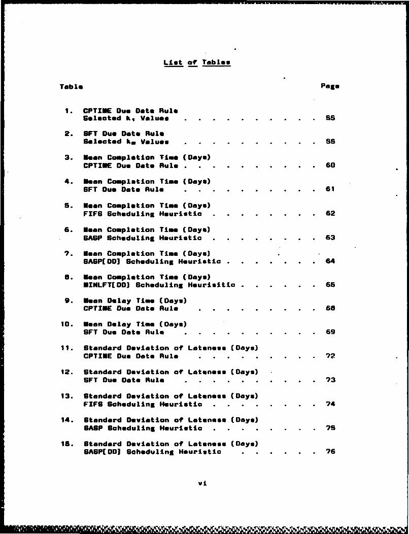
List of Tables

Table Page

I. CPTIUE Due Date RuleSelected kv Values . . . .. . . . . . 99

2. OFT Due Date RuleSelected ka Values . . - . . . . 56

3. Meon Completion Time (Days)CPTIEE Due Date Rule . . . . . . .. . . 60

4. Mean Completion Time (Days)OFT Due Date Rule . . . ..... . . 61

S. Mean Completion Time (Days)FIFS Scheduling Heuristic . . . . . . . 62

6. Mean Completion Time (Days)GASP Scheduling Heuristic .. . . . . . . 63

7. Mean Completion Time (Days)SASPL 001 Scheduling Heuristic . . . . . . .64

0. Mean Completion Time (Days)*INLFT(DDJ Scheduling Hourisitic . . . . .. 65

9. Mean Delay Time (Days)CPTIUE Due Date Rule . . . . . . .. 68s

10. Mean Delay Time (Days)OFT Due Date Rule .. . . . . . . . . 69

11. Standard Deviation of Lateness (Days)CPTIME Due Date Rule . . . . . . . . 72

12. Standard Deviation of Lateness (Days)OFT Due Date Rule .. . . . . . . . . 73

13. Standard Deviation of Lateness (Days)FIFO Scheduling Heuristic . . . . . . . . 74

14. Standard Deviation of Lateness (Days)GASP Scheduling Heuristic. . . . . . . 75

15. Standard Deviation of Lateness (Days)SASP(D Scheduling Heuristic . . . . . . 76

vi

Table Page

16. Standard Deviation of Lateness (Days)

MINLFT[DDO Scheduling Heuristic . 7?

17. Mean Tardiness (Days)CPTIUE Due Date Rule . . . . 81

IS. Mean Tardiness (Days)OFT Due Date Rule . . . . . 82

19. Mean Tardiness (Days)FIFS Scheduling Heuristic . . . . . . 83

20. Mean Tardiness (Days)SASP Scheduling Heuristic . . . . . . . . 84

21. Mean Tardiness (Days)SASP[DDJ Scheduling Heuristic . . . . . . .85

22. Mean Tardiness (Days)MINLFT[DD] Scheduling Heuristic . . . . . 86

23. Mean Completion Time (Days)Uniform Arrival Distribution . . . . . . . 91

24. Mean Completion Time (Days)Exponential Arrival Distribution 92

25. Mean Completion Time (Days)Triangular Arrival Distribution . . . . . 93

26. Standard Deviation of Lateness (Days)Uniform Arrival Distribution . . . . . . 94

27. Standard Deviation of Lateness (Days).Exponential Arrival Distribution . . . . . 95

28. Standard Deviation of Lateness (Days)Triangular Arrival Distribution . . . . . . 96

29. Mean Tardiness (Days)Uniform Arrival Distribution . . . . . 9?

30. Mean Tardiness (Days)Exponential Arrival Distribution . . . . . 98

31. Mean Tardiness (Days)Triangular Arrival Distribution . . . . . 99

32. Three Factor ANOVA TableMean Completion Time . . . 116

vii

Table Page

33. Three Factor ANOVA TableMean Delay Time . . . . . . . . . . . 123

34. Three Factor ANOVA TableStandard Deviation of Lateness . . . . . . 130

35. Three Factor ANOVA TableMean Tardiness . . . . . . . . . . . 13?

Vill

AFIT/ SU/LY/S7-19

Abstract

This research addresses the issue of what impact

differences in project arrival distribution may have on

procedures for setting due dates and scheduling project

activities to mat those due dates in a dynamic, multi-

project, constrained multiple resource, environment. In

general it was found that different project arrival

distributions do affect the performance of scheduling

heuristics and due date sotting rules in an absolute sense,

but not in 4 relative sense. Because of this, the project

manager does not really need to be concerned about the

arrival distribution of new projects because the relative

performance of the tested heuristics and due date assignment

rules is the same.

The best results are obtained when the Scheduled Finish

Time (BFT) due date setting rule is applied. Not only does

it provide the most accurate due dates, it provides

significantly better results when used with any scheduling

heuristic than the other due date setting rules, and it is

virtually not affected at all by differences in project

arrival distribution. Every project manager probably dreams

of such a procedure being available, however there is a

price to pay for the SFT due date assignment rule. The SFT

due date setting rule requires a finite scheduling system,

the current status of all projects in the system, and a

ix ]

Mt W

historical data base to establish the due date compensation

factor ("k" value). Not all project managers could

implement this procedure due to the computer

hardware/software requirements, financial constraints,

project duration uncertainty, resource constraints, eta..

If they could use the SFT rule to set the due date of the

arriving project, they would be wise to use the very simple

First-In-First-Served (FIFG) scheduling heuristic to

allocate resources to the project.

An alternative to project managers would be to choose

the easier to implement CPTIUE due date rule. If this Is

the case then the manager would want to choose one of the

due date oriented heuristics to schedule the activities.

The GASP(DO] and MINLFT(D] produce similar results using

the CPTIME duo date rule. The CPTIME due date setting rule

ignores the current project load when estimating activity

completion times and therefore lacks the "self-compensating"

feature of the SFT due date assignment rule.

Recall that the goals of the project manager are to

first of all determine reasonable due dates for each project

in .order to make a promised completion date to the customer

and then schedule those projects accordingly so that due

dates are met on time. This research has determined that

the relative performance of the tested scheduling heuristics

and due date setting rules is unaffected by the project

arrival distribution. For the project manager, this

x

confirm* that certain scheduling heuristics, due date

assignment rules, and combinations thereof will perform

better then others regardless of the project arrival

distribution. Therefore, the alternatives to management are

1) accept the decrease In performance capability for the

eaier to Implement CPTIME due date assignment rule used

with the due date oriented heuristics; or 2) make the

necessary commitments and Investments to Implement at least

one of thee heuristic. combined with the OFT due date

assignment procedure or better yet; 3) Implement the

FIFS/9FT combination for assured performance.

X1

AN EVALUATION OF PROJECT SCHEDULING

TECHNIQUES IN A DYNAMIC ENVIRONMENT

I. Introduction

Projects have been part of the human soene since

civilization started yet the preatice of project management

Is, on the historical timeucale, almost brand now. Only In

the lost couple of decades has the subject appeared to any

extent In manegemnt literature. Current budgeting and

planning methods are all relatively recent, Perhaps the

reason for emphasis on project management Is that It is

osnoerned with the management of resources, Including the

met expensive resource of all - namely the human resource.

It io no longer the case that a few thousand slaves can be

deployed to build some architectural extravagance regardless

of their welfare and safety. Almost everything now depends

on time and cost constraints. Moreover, there is

competition. If one contractor fails to meet its obligations

or targets, no doubt twenty others will be ready to jump in

to take Its place when the next job comes up. Management

has been described as "getting results through people".

Amend that definition to *achieving successful project

completion with the resources available" and you have

a succinct definition of project management, the

resources being time, money, materials and equipment, and

people (12:3).

General Issue

Efficient project management requires more than good

planning. It requires that relevant information be obtained,

analyzed, and reviewed in a timely manner. This can provide

early warning of pending problems and impacts on related

project activities thereby providing the opportunity for

alternate plans and management actions. Today, project

manager. have access to a vast array of software packages to

assist them in the difficult task of planning, tracking, and

controlling projects. Many of the more sophisticated

project scheduling software packages that previously

required mainframe computer support are now available for

microcomputers.

Most, if not all, academic and commercial software

designed for project scheduling salve only the static,

unconstrained resource, project scheduling problem. The

static scenario consists of scheduling a oet of known

activities, such that each activity begins only after its

preceding activity is completed. Resources to accomplish

each took are unconstrained. The problem of interest to

most project managers, in this poenario, is sequencing the

activities to minimize the project's duration (UOsig

critical path methodology). However, resources In reality

2

are constrained which may cause concurrent activities to be

delayed end cause an increase in project duration.

The static, multi-projeat, constrained resources

problem Is characterized as having many projects present,

each having the some starting point but having different

stopping times for the different projects. As an example,

a construction company planning to build several buildings

at the same time is faced with the static, multi-project,

constrained resources problem. The solution to this

particular type of scheduling problem is a schedule which

allocates the limited resources to the activities of the

multiple projects so as to minimize the individual project

completion times (5:6).

A much more challenging class of project scheduling

problems confronting today's managers consists of multiple

projects that arrive indefinitely over time with a given

level of resources available to the project manager. In

this dynamic environment the project manager must estimate a

project completion date (due date) for each project as it

arrives and then take scheduling actions to meet this date.

This task is relatively simple in the static, multiple

project environment with unlimited resources and the

technique used to ensure the due dates are met in the

minimum amount of time is most likely a critical path

methodology. However, the task of meeting due dates and/or

minimizing project completion times becomes much more

3

complex in the dynamic, multiple project with constrained

resources environment.

Many organizations face the problem of managing

multiple projects requiring multiple resources. One oamon

planning factor they all face is deaiding a completion date

(due date) for each individual project that is attainable

and can be promised to a customer, reaognizing now projects

will arrive in the future which will add to the existing set

of projects and compete with the organization's limited

resources. Each organization has some historical basis for

estimating completion times of familiar projects and

therefore develops a technique for estimating project due

dates. Once the due date is established, activity control

decisions (scheduling) need to be made on the assignment of

resources to minimize deviations from the promised due

date (6:4).

Research in this area of project scheduling has not

been pursued as extensively as the static, multiple project

scheduling problem. Some techniques have been developed for

scheduling multiple projects in a dynamic arrival

environment where the resources are limited. Various due

date setting rules are available and scheduling heuristics

are used in meeting due dates. A computer simulation model

has been developed to evaluate the effectiveness of

techniques for scheduling multiple projects in a dyntamic,

multi-project, constrained resources environment (8).

4

Sckground

Planning, scheduling, and control are three of

the most important functions of management and project

managers strive for techniques to accomplish these

functions more effectively especially when a complex set of

aotivities, functions, and reletionshipu is involved.

Networking models have proven to be extremely useful in the

static project environment for the purpose of tracking tite

performance of large and complex projects.

Two networking tools that have been used frequently

by managers are: 1) the Program Evaluation and Review

Technique (PERT); and 2) the Critical Path Method (CPU).

PERT/CPU was designed to eliminate or reduce production

delays, conflicts, and interruptions in order to coordinate

and control the various activities within a given project

and to assure completion of the project on the scheduled

date. Many projects are complex and consist of many highly

interrelated activities and events which make coordination

and control of the entire project difficult. roday, project

managers have access to a large array of PERT/CPU software

packages to help in the difficult task of tracking and

controlling projects (11:89).

Urigin of Part (6:?). PERT was developed in 1986

by the U.S. Navy for the Polaris missile program. The

Polaris program had over 60,OUU definable activities which

had to be accomplished by over 38OU contractors, suppliers,

5

and government agencies. A project of this magnitude and

complexity had never been attempted before, making it very

difficult to predict oompletion times of critical tasks or

track the progress of the overall project. Therefore,

PERT was specifically designed to handle uncertainties in

activity duration times. PERT requires three estimates of

the duration for each activity ( optimistic, most likely,

and the pessimistic). By the use of a Beta distribution

function, these three estimates are refined to one expected

time and its variance.

Oriain of CPI (8:8-9). CPS was developed in 195?

priarily by DuPont Corporation and Remington Rand. The

chemical Industry was interested in being able to provide

time and cost trade-offs in building, overhauling, and

maintaining chemical plants. If there are unlimited

resources, the longest direct route through the project

network is the critical path. The minimum time required to

complete the project is the sum of the durations of all the

activities along the critical path. Any delay in these

critical activities will delay the final project completion

date. The program manager's task is to ensure that the

resources required for the critical aotivities are available

on a timely basis and that the project is complatd in

its critical path time. Proper control and diroction of the

activities comprising the critical path iLve mandgers

innight to the time and costs involved in a project of any

6

size. The CPO technique makes an assumption that activity

duration times are deterministic (single time estimate for

each activity). It offers the option of-increasing

resources, usually at increased costs, to decrease certain

activity times. The distinguishing feature between PERT and

CPU is that CPO provides time and cost trade-offs for

activities within the project.

Network Applications (6:11-13). In both the PERT

and CPU models the basic procedure consists of five steps:

1) analyze and break down the project in terms of specific

activities and/or events; 2) determine the interrelation-

ships and sequence of activities and produce a network; 3)

assign estimates of time, costs, or both to all activities

of the network; 4) identify the longest or critical path

through the network; and 8) monitor, evaluate, and control

the progress of the project by replanning, rescheduling and

reassignment of resources. The primary task is to

determine the critical path through the network (minimum

project duration time). If the project must be completed in

less time then the critical path, those activities along the

critical path must be re-analyzed in terms of what resources

must be dedicated to expedite one or more activities along

the critical path. Non-critical paths are more flexible in

scheduling and distribution of resources, because they take

less time to complete than the critical path. The

networking process signals the project manager when the

W M 11110 1 11%1% 111 1 1,1W 111 11W M IM 7N

critical path of the project is placed in jeopardy. The

manager must then take the appropriate actions in order to

compensate for any delays.

PERT and CPU can be used for many types of projects,

but the emphasis of these models is on the static project

environment (single or multiple one-time projects).

Resource Constraints in Static Project Scheduling

(13:191-213). Resource availabilities are not considered

in the basic PERT/CPU scheduling process and therefore are

somewhat limited in producing a detailed project schedule.

PERT/CPM procedures implicitly assume that the resources are

unlimited and that only precedence relationships between

activities constrain activity start/stop times. One

consequence of this is that the schedules produced may not

be realistic when the resources are constrained. Because of

this, the basic time-only PERT/CPm forward-backward pass

procedure has been called by some "a feasible procedure for

nonfeasible schedules."

Resource constraints alter and complicate some of the

basic principles of PERT/CPU. For example, the longest

sequence of activities through any one project when

resources are constrained may not be the same critical path

determined by the basic time-only PERT/CPU technique. While

under resource constraints many different Early Start time

(ES) schedules may exist, whereas there is only one unique

EG schedule in the basic time-only PEHT/CPU approach. ro

understand these differences it is necessary to see how

limited resources affect schedule slack (float).

How Limited Resources Affect Schedule Slack.

Figure 1 shows a simple activity network with activity times

indicated beside each node. FZvgure 2a shows the all-ES

bar chart schedule for this network, assuming that the

resources are unlimited. The project duration is 18 weeks,

the critical path is the activity sequence A-C-I-J-K, and

activities B, 0, E, F, 9, and H all have positive slack.

Now assume that jobs C and G each require the same

resource, say a hoist crane, but only one crane is

available. Also, assume that jobs E and F require a special

bulldozer, but only one is available.

The result of these simple resource constraints is that

neither jobs C and 9 or jobs E and F can be performed at the

same time as indicated previously In Figure 2a. One or

the other of these activities will be given priority and

each pair must be sequenced so there Is no overlap (see

Figure 2b).

When resources for activities C and G and E and F are

constrained, the following results occur:

1. Activities 0 and H become critical, with slack

reduced to zero.

2. Activities 0, E, and F have their slack reduced

considerably.

9

A3 J K Dumm

2 3 2 finis

0 10 ~ t no.1

Figure 2.. USimited RctiviurcetScedul (13:19)

A

CJ

lid na, but Onl rane

WA and -" * o F ec

i~~t Is p I I I

Figure 2a. Ulimited Resources Schedule (13:193)

A'

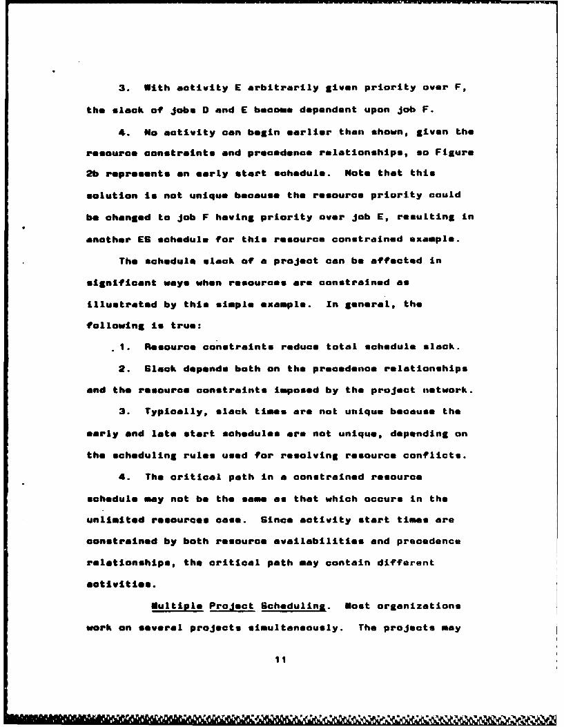
3. With activity E arbitrarily given priority over F,

the slack of Jobs 0 and E become dependent upon job F.

4. No activity can begin earlier than shown, given the

resource constraints end precedence relationships, so Figure

2b represents an early start sohedule. Note that this

solution is not unique because the resource priority could

be changed to job F having priority over job E, resulting in

another ES schedule for this resource constrained example.

The schedule slack of a project can be affected in

significant ways when resources are constrained as

illustrated by this simple example. In general, the

following is true:

1. Resource constraints reduce total schedule slack.

2. Slack depends both on the precedence relationships

and the resource constraints Imposed by the project network.

3. Typically, slack times are not unique because the

early and late start schedules are not unique, depending on

the scheduling rules used for resolving resource conflicts.

4. The critical path in a constrained resource

schedule may not be the same as that which occurs in the

unlimited resources case. Since activity start times are

oonetrained by both resource availabilities and precedence

relationships, the critical path may contain different

aotivities.

Multiple Project Scheduling. Most organizations

work on several projects simultaneously. The projects may

11

7. .N

be at different locations and may be represented by

independent networks. These projects frequently require

some of their resources to be drawn from a common pool.

Engineers, draftpersons, equipment, etc. are some examples

of shared resources within a company (12:403).

When a company is handling several projects at the same

time and where the resources must be shared between

projects, it is necessary to integrate the planning and

control of these multiple projects. Some examples of this

situation are (10:131-132):

1. A large chemical company which has several major

projects occurring simultaneously, each at various phases in

its. life cycle and each probably with a different

contractor.

2. A contractor who has several projects with

different client companies.

3. A factory with a variety of small and medium sized

projects, using its own resources and sometimes for large

projects, using subcontractors or contractors.

Eulti-projeot scheduling has to accommodate for

resource availabilities in the common resource pool and for

the resource availabilities assigned to specific projects.

When several projects are being scheduled under constrained

resources, one has to consider the priority of these

projects (12:403).

12

The impact of resource constraints on scheduling in the

single-project illustrated above increases significantly for

scheduling multiple projects. Figure 3 shows a hypothetical

three-project scheduling scenario involving just three types

of resources. To simplify this example, activities

requiring a resource use only one unit of any one of the

three types of resources, and only one of any type is

available.

Prsjm 1 Proem 2 Prom 3

1 4

• . .,/ I--I

31

' !,

,',t

Rusues ITimeTime

Figure 3. Multiple Project Schedule (13:198).

13

A domino series of events might occur as a result of

delaying activities to resolve resource conflicts as they

occur. For example, delaying activity 1-3 of project I (to

resolve the conflict with activity 1-3 of project 2) might

cause the following (13:192-193):

1. Delays in successor activities 3-4, 3-5, and 4-5 of

project 1.

2. As a result of (1), the creation of additional

resource conflicts among activities requiring resource types

2 and 3 to be resolved.

3. As a result of (2), additional delays in projects 2

and 3, and possibly even project I again.

Developing and maintaining schedules for multi-project

problems, involving many projects, a variety of resource

types, and thousands of activities, are possible only with

the aid of powerful computers. The point being, the

aspect of resource constraints elevates the complexity

of the multi-project problem from a relatively simple

exercise using the basic time-only PERT/CPU approach to a

much more challenging problem of immense proportions that

requires sophisticated computational routines and powerful

computers to solve.

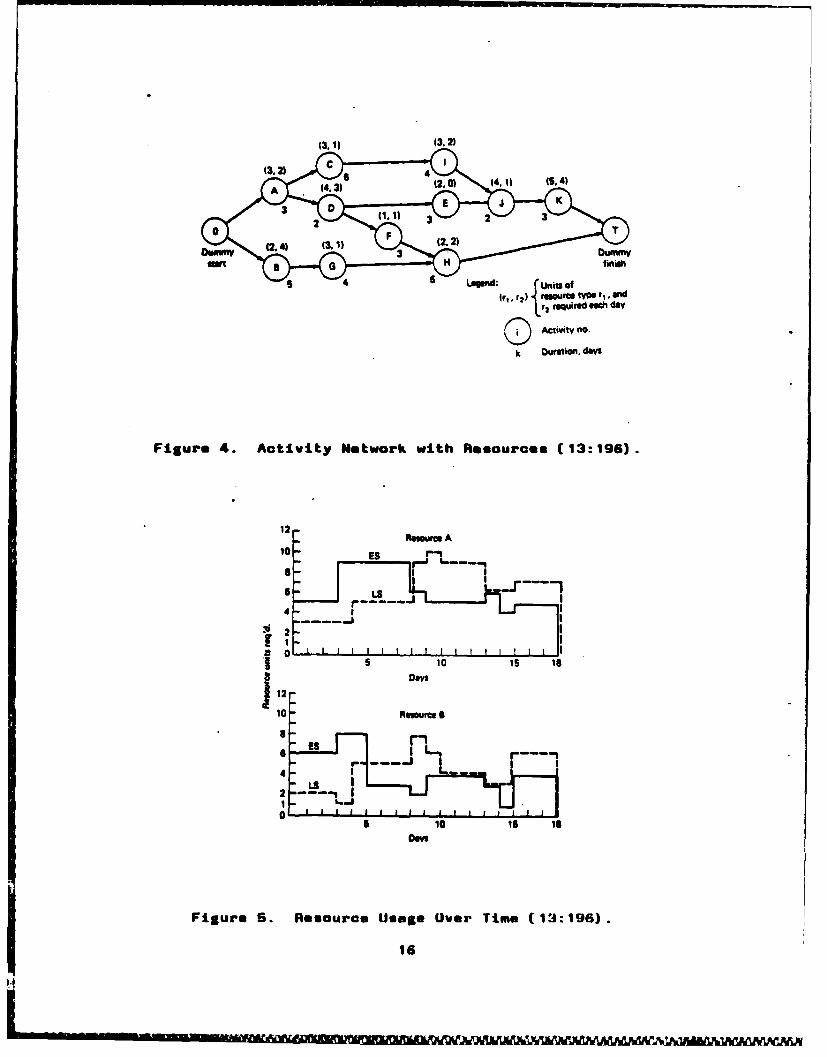
Resource Loadins. The network model for project

scheduling lends itself readily to information about

resource requirements over the duration of the project.

The only condition for obtaining this information is that

14

the resource requirements associated with each project

activity shown on the network be identified separately (see

Figure 4).

Figure 4 is the same network as shown in Figure 1 with

resource requirements of two different types indicated above

each activity. By using these resource requirements

together with an early start (see Figure 2) and a late start

schedule (not shown) a plot of resource usage over time can

be developed as shown in Figure 5. These plots are referred

to as resource loading diagrams. Such diagrams are very

useful in project management; they highlight the period-by-

period resource usage of a specific project schedule and

provide a basis for qanagers to improva scheduling

decisions.

Basic Scheduling Procedures for the Resource

Problem (13:202). Scheduling procedures for dealing with

the resource constrained problem can be divided into two

basic categories: 1) resource leveling, and 2) constrained-

resource scheduling. Resource leveling occurs when

sufficient total resources are available, the project must

be completed by a promised due date, but It is desired to

reduce resource usage variance over the duration of the

project. A constant level of resource usage is desired and

the project duration is not allowed to increase in this

case.

15

e,

(3.1) 13."2)auO tO r1 n

5~~~1 18 eed: Uiso

0 Acivt no.I

Figure 4. ActiityNeork withe Oeouime (1:196).

I 16

The more common and most Interesting problem arises

when resouroes are constrained. The soheduLing objective in

this case is to meet project due dates as much as possible,

subject to the fixed limits on resource availability. Thus,

projeot duration may increase beyond the initial due date

determined by time-only PERT/CPU calculations. The

scheduling objective is to minimize the duration of the

project (or projects) being scheduled, subject to the

constraints imposed by limited available resources. This

problem can be further subdivided into two categories

according to whether the fixed limits on resource

availabilities are. constant at some level or allowed to

change over activity or project duration. Further

subdivisions are possible according to whether approximate,

rule-of-thumb procedures, or mathematical exact procedures

are used to solve the scheduling problem.

Heuristic Schedulins (13:202-21?). The task of

scheduling a set of project activities such that both

resource constraints and precedence relationships are

satisfied is not easy. The difficulty is increased in the

multi-project environment. The limited resources, project

scheduling problem falls into a category of mathematical

problems called combinatorial problems. Analytical methods

such as mathematical programming have not proven very

successful on this clams of problems. Instead, heuristic

1?

procedures hae been developed and are being used to solve

these problems.

Heuristics are 'rules-of-thumb" that reduce the

computational effort Involved in project scheduling. They

may not always provide the optimal solution In every case,

but they are very useful in finding a good solution with

minimum effort.

Simple heuristics such as "shortest job first" or

aminimum slack first' are effective In establishing

priorities on many types of resource-constrained scheduling

problems. More sophisticated heuristic procedures exist

and are described in further detail In the literature

review.

Although individual studies have indicated the general

best effectiveness of a particular heuristic, or combination

of due date assignment rule and scheduling heuristic, It

must be emphasized that It has been shown that no one

heuristio-or combination of heuristics-always produces the

best results on every problem. This Is perhaps the greatest

disadvantage of using scheduling heuristics. In practise,

even with very sophisticated procedures, it is not possible

to guarantee the performance across the board of any one

heuristic or combination thereof.

Despite this disadvantage, heuristic scheduling

procedures are used often in practice. The schedules

produced by these teohniques may not be optimal, but they

18

are good enough for planning and control purposes in view of

the uncertainties associated with activity durations,

resource constraints and requirements. Some very powerful,

oomputer-based solution procedures Incorporating a variety

of creative heuristics have been developed which

produce schedules for large, complex projects under a

variety of assumptions. The most challenging problem of

course is the dynamic, multi-project, multiple resource

project scheduling problem which has received very little

academic attention.

The Dynamic Versus Static, Multiple Resource, Multi-

Project Soheduling Problem (5:1-13). Resource-

constrained project scheduling research has been limited

almost exclusively to the static problem where all aspects

of the projects are assumed a priori. The emphasis being on

finding scheduling techniques which minimize project

completion time. The result is a master schedule which

allocates specified quantities of the required resouroes to

certain activities at certain times. In reality, the

project scheduling environment is dynamic; new projects

arrive but the exact arrival times of future projects, their

activity duration times, and their resource requirements are

uncertain and not known until it arrives. These major

differences delineate the static versus the dynamic,

multiple resource, multi-project scheduling problem.

Standard project scheduling techniques dre inadequate in the

19

1*1 V R.,15

dynamic environment because they are unable to schedule

resources to projects for which there Is no Information.

In general, project managers are faced with two

problems in project scheduling. First, they must estimate a

realistic and minimum expected project completion date (due

date). Second, they must schedule this project to mat this

due date while not seriously jeopardizing the completion of

engoing projects.

Estimating a realistic due date for a project involves

detailed knowledge of the project and depends on:

1. The characteristics of the project (number of

activities, successor-predecessor relationships, activity

duration times, resource requirements, etc.).

2. The current load of projects in the organization.

3. The future load in the system (as impacted by

additional projects).

4. The scheduling heuristics used to allocate the

resources to the projects.

The goal of a project manager is to make good estimates

of project completion times and deliver the product or

service on time to the oustomer.

good due date setting rules and scheduling heuristics

have been explored recently by simulating the dynamic,

multiple resource, multi-project problem with a computer

based model (5). The focus of this research is a

continued exploration of the performance of these due date

20

setting rules and scheduling heuristics under variations in

the assumptions of the arrival rate distribution.

Specifto Problem Statement

Many organizations, both commeroial and government,

operate In a multiple project environment where their

resources are constrained and new projects arrive on a

continuing basis. These organizations are expected to

estimate a completion date on each of these new projects and

then take scheduling (management) actions to met these

estimated completion dates.

The specific problem of estimating due dates and

scheduling multiple projects in a dynamic, resource

constrained environment has not received much attention

academically or commercially. Because of the difficulty of

the problem, previous research has focused almost

exclusively on the static project environment with the

purpose of finding scheduling methods that minimize the

completion time of the project. Project managers have

access to a large assortment of commercial software programs

which basically provide a common schedule, allocating

specified amounts of resources to activities at the required

time In order to mast the minimum project completion date.

However, these techniques require that all aspects of all

projects be known in advance. Realistically, in a dynamic

environment, the requirements and arrival time of new

projects are not known in advance. This basic difference

21

makes standard project scheduling models inadequate in a

dynamic environment. rhere are three significant

differences between the static and dynamic project

environment (8:6).

static Dynamic

1. Finite number of projects 1. Unknown set ofin advance. projects to be scheduled

over time.

2. All projects start at 2. Projects arrive at anytime zero and all character- time and the character-istics (activities, durations, istics are unknown untilresources, etc.) are known in their arrival.advance.

3. Start with resource at 3. Resources are con-zero, go to a peak resource strained at a given levellevel, and return to zero. and remain constant

throughout time.

Dumond identified several areas of future research on

the dynamic, multi-project scheduling problem. A particular

area of interest to this researcher is the environments used

by Dumond to evaluate due date setting rules and scheduling

heuristics in a simulated dynamic project arrival

environment. The problem of interest is to examine the

sensitivity of the performance of these due date setting

rules and scheduling heuristics under variations In the

assumptions regarding the project arrival distribution.

Research Objective

The overall objective of this research is to

Investigate the Impact of differences in project arrival

distributions during a simulation of the dynamic,

22

multi-project scheduling environment on the performance of

the due date assignment rule and scheduling heuristic

combinations Investigated previously by others. To achieve

this objective, the following research questions should be

answered:

1. Are scheduling heuristics, investigated in previous

research, impacted by whether new projects arrive according

to a uniform, exponential or triangular distribution?

2. Are due date setting rules, investigated In

previous research, impacted by whether new projects arrive

according to a uniform, exponential or triangular

distribution?

3. Is any combination of scheduling heuristic and due

date setting rule, Investigated in previous research,

impacted by whether new projects arrive according to a

uniform, exponential or triangular distribution?

Scope of the Research

The scope of this research concentrates first on

reviewing the due date setting rules and scheduling

heuristics evaluated by Dumond and others (5). Then-an

Investigation of the details of the computer-simulation

model used to evaluate the effectiveness of these dynamic

scheduling techniques will be conducted. Finally, the major

thrust of this research effort will be to explore various

dynamic project environments to test the generalizability of

the results presented in (5, 6) and answer the research

23

questions Identified above. The investigation and

simulation of other project arrival distributions will

hopefully add to the robustness of the existing results and

demonstrate the sensitivity of the due date assignment rule

and scheduling heuristic combinations to project arrival

distributions.

24

IZ. Research Methodology

The general methodology will focus on collection of

data pertaining to the evaluation of the effect of different

project arrival distributions on the performance of selected

due date assignment rules and schaduling heuristics in the

dynamic, multiple resource, multi-project scheduling

environment. The initial portion of the research will be an

extensive review of the literature on the dynamic, multiple

resource, multi-project scheduling problem to determine if

this problem Is being actively pursued and what types of

project scheduling criteria or rules are being developed to

address the dynamic project environment. Since a simulation

model has already been developed (5), it will be of

interest to the researcher to determine how the model must

be modified and installed on the local computer facility in

order to simulate the effect of different project arrival

distributions on the performance of several combinations of

interest of due-date assignment rules and scheduling

heuristics. The objective being to determine if there is

any significant difference in the performance of these due

date assignment rules and scheduling techniques and if so,

are these differences attributable to the difference in the

project arrival environment.

This chapter further establishs a rationale for

Investigating the problem, provides a review of current

literature in this field of study, proposes an appropriate

25

'I

experimental design to address the problem and collect data,

desoribes the fundamental characteristics of the computer

simulation model to be employed in this investigation, and

finally, addresses the method of data analysis proposed for

this experiment.

Experimental Approach

The primary rationale for investigating this problem is

based upon the recommendation by Dumond for further

exploration of the environments used in his experiment-

ation (5). The arrival distribution and mean interarrival

rate was held fixed during the experiments and the

recommendation was made to pursue other distributions and

arrival rates (5:195). Dumond used a uniform project

arrival distribution with a mean interarrIval rate of one

new project every 8 days. The main experiment consisted of

a two-factor full factorial design to determine the

performance of four due date setting rules and seven

scheduling heuristics under one set of environmental

conditions (5:70). The project arrival distribution and

mean interarrival rate were not factors in Dumond's

experimental results.

Project Arrival Distributions. In order to make a

comparison of experimental results with Dumond's previoas

study, a replication of the experiment using a selection of

two due date setting rules and four scheduling heuristics

will be performed using three different project arrival

26

distributions (uniform, exponential, and triangular).

Priteker states the following an the uniform distribution

(17:696-697):

The uniform density function specifies that every valuebetween a minimum and a maximum value is equally likely.The use of the uniform distribution often implies a completelack of knowledge concerning the random variable other thanthat it is between a minimum value and a maximum value.Thus, the probability of a value being In a specified

interval Is proportional to the length of the interval.Another name for the uniform distribution is the rectangulardistribution.

Figure 6 gives the density function and its graph for the

uniform distribution.

ffx)" ;asxs.bb-a

aa+ b r (bAzle2 12

1

a b

Figure 6. Uniform Density Function (17:696)

Most of the queuing theory literature pertains to the

special case when job interarrival times are a series of

independent, observations from an exponential distribution.

Meaning, the number of arrivals in a given period of time is

a random variable with a Poisson distribution. This is

referred to as the Poisson process and in queuing theory is

referred to as Poisson arrivals. Poisson arrivals are used

quite frequently in queuing models because it is a reason-

2?

able reprementation of many physical prooesses, but a more

important reason is because of the tremendous analytical

convenience that the Poisson process provides (4:142-151).

Pritaker states the following about the exponential

distribution (17:69?-698):

If the probability that one and only one outoome willoccur during a small time interval Is proportional to thissmall time interval and if the occurrence is independent ofthe occurrence of other outcomes then the time betweenoccurrences of outcomes is exponentially distributed.Another way of saying the above is that an activitycharacterized by an exponential distribution has the someprobability of being completed In any subsequent period ofan equal small time interval. Thus, if the activity hasbeen ongoing for t time units, the probability that it willend in the next time interval is the same as if it had justbeen started. This lack of conditioning of remaining timeon past time is called the Markov or forgetfulness property.There is direct association between the assumption of anexponential activity duration and Markovian assumptions.The use of an exponential distribution assumes a largevariability as the variance is the square of the mean. Theexponential has one of the largest variances of the standarddistribution types. The exponential distribution is easy tomanipulate mathematioally and is assumed for many studiesbecause of this property.

Figure ? gives the density function for the exponential

distribution and a graph of the distribution.

0 . f(X)- X e - >0\2.Ix) OLS

1.0

0- 2.0

Figure ?. Exponential Density Function (17:698)

28

'I

Therefore a rationale can be established for exploring

the performance of due date setting rules and scheduling

heuristios assuming a Poisson arrival process and,

therefore, an exponential project arrival environment.

An argument can also be made that job arrival times are

perhaps a sequence of independent observations from a fixed

normal distribution. An environment may exist which closely

resembles the static, multiple resource, multi-projeat

problem such that the nature of project arrivals are fairly

repetitive and predictable for a particular organization,

however iomn uncertainty remains In the variability of

project arrivals. Therefore, one may assume that a normal

distribution of project arrival times is appropriate for

modelling the dynamic, multiple resource, multi-project

problem. The difficulty remains in selecting the

appropriate variance and, hence, standard daviation for a

normal process of project arrival times. Also, a

complicating feature of the normal distribution Is the

infinite tails of the distribution which could be solved by

truncating the distribution. A triangular probability

distribution can be used as a reasonable approximation of

the normal distribution that does not require knowledge of

the variance or standard deviation, only the minimum, mode,

end maximum value of probable project arrival times. The

triangular distribution resolves the need for truncating the

29

I A I

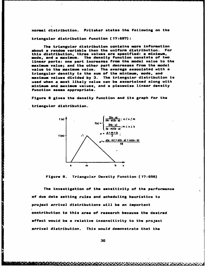
normal distribution. Pritzker states the following on the

triangular distribution function (17:697):

The triangular distribution contains more informationabout a random variable then the uniform distribution. Forthis distribution, three values are specified: a minimum,mode, and a maximum. The density function consists of twolinear parts: one part increases from the modal value to themaximum value; and the other part decreases from the modelvalue to the maximum value. The average associated with atriangular density is the sum of the minimum, modes, andmaximum values divided by 3. The triangular distribution is

used when a most likely value can be ascertained along withminimum and maximum values, and a piecowis linear densityfunction seems appropriate.

Figure 8 gives the density function and its graph for the

triangular distribution.

f (x) (x )(- a) ; 8. 1 a Mffx) 2(b- x) ;m X b

I (b- m4b- a- )(m)l.

/ , a(a-m)+b(b-)+m(m-b)

a m b x

Figure 8. Triangular Density Function (17:698)

The investigation of the sensitivity of the performance

of due date setting rules and scheduling heuristics to

project arrival distributions will be an important

contribution to this area of research because the desired

effect would be a relative Insensitivity to the project

arrival distribution. This would demonstrate that the

30

ON

combinations of due date setting rule and scheduling

heuristic would not need to be compensated for the

particular type of project arrival distribution and, hence,

would remain good rules of thumb for scheduling projects in

the dynamic, multiple resource, multi-project environment.

Limitations. The most significant hurdle anticipated

will be trying to install the simulation model on an

accessible mainframe computer, debugging the model, and

conducting a protest of the model using existing date. Once

the simulation is installed, it should be a reasonably

straightforward process to acquire new data (different

project environments, scheduling rules, etc.) and to

evaluate the effectiveness of various due date assignment

rules and scheduling techniques in a dynamic project arrival

environment.

Literature Review

A review of current literature has revealed that very

little research effort has been directed towards the

dynamic, multiple resource, multi-project scheduling

problem. Several related articles were discovered that

addressed heuristics and due date rules for resource

constrained scheduling problems, but none specifically

addressed the dynamic, multiple resource, multi-project

scheduling problem (1, 2, 3, ?, 9, 16, 18). The most

relevant current research effort was conducted by Dumond

31

whiah provides the foundation of this experimental

investigation (5).

The remaining discussion will be an overview of the due

date setting rules, scheduling heuristics, and performance

measures that apply to the methodology to be incorporated in

the experimental design.

Due-Date Assignment Rules. A due date is defined

as the present date plus an estimate of the amount of time

required to complete a project. Meeting an assigned due date

is considered a major performance criterion in project

management. Due date assignment rules can very from simple

to sophisticated depending on the degree of information

known and used about a project's characteristics and the

status of the system at the time of project arrival. Dumond

investigated the folLowing four due date rules (6:10-12):

1. Mean Flow Due Date Rule (FLOW).

2. Number of Activities Due Date Rule (NUMACT).

3. Critical Path Time Due Date Rule (CPTIME).

4. Scheduled Finish Time Due Date Rule (9FT).

The letter two rules are the more sophisticated and are

considered as the two treatments for the due date rule

factor of the three-factor experimental design.

Critical Path Time Due Date Rule (6:11). The

critical path of a project determines the time to complete

the project given that resources are not constrained. This

rule considers the activity predecessor relationships of the

32

project and the duration of the critical activities of that

project. Since resources are constreined in this problem an

adjustment to made to the criticel path time due date

estimate by multiplying the critical path time estimate by a

delay factor based on historical date. This adjusted value

beooames a more realistic estimate of the project's

completion time end Is used to set a due date for that

particular project. CPTXIE is given by the following:

DOs - TNO * k, * CPTMEa (1)

where

CPTIUE5 - critical path time of project I

kv - parameter representing expected delay

Scheduled Finished Time (6:11-12). This rule

finitely schedules a new project into the system along

with current projects in the system before setting a due

date. Therefore, start and stop times of each activity of

each project is established. The scheduled finished time of

the lost activity of the arriving project is an excellent

estimate of the completion time of the new project provided

no new projects arrive. In the dynamic project environment

new projects will continue to arrive and the scheduled

finish time Is usually not met. Therefore, the estimate

must be oompensated by an appropriate delay factor.

The OFT technique involves the following three steps In

order to set the due date for a new arriving project:

1. Temporarily set the due date of the new Incoming

33

project as the current date plus the computed critical path

time of the now project, without regarding resource needs.

2. Sohedule the remaining activities of all current

projects in the system plus those activities of the new

project using the selected scheduling heuristic (i.e.9

first-in-first-served, shortest activity of shortest

project, etc.).

3. Set the permanent due date of the new project as

the present date plus a delay factor (k2) times the

estimated completion time for the new project.

The SFT due date rule is given as follows:

DOO - TNOW + km(SFT(E)a - TNOW) (2)

where

ko - the expected delay factor

9FT(E)& - the estimated scheduled finish time forproject I after loading

(9FT(E)& - THMU) - estimated completion time for thenew project

The OFT due date rule determines the early activity start

times of the new project based upon resource constraints at

the time. Therefore, the same project arriving at different

times but using the same SFT heuristic would be assigned two

different estimates of their completion times. In other

words, if the system is relatively empty a shorter due date

will be assigned than if the system is relatively full.

34

Scheduling Heuristics (6:6-9). Project

scheduling heuristics allocate the constrained available

resources based on a prioritized list of the competing

ectivities from one or more projects. Some heuristics

perform better then others in reducing the mean completion

time of projects. By assuming that the dynamic, multiple

resource, multi-project problem consists of a series of

static problems, then one can use these same heuristics in

the dynamic environment. Dumond investigated the

performance of several scheduling heuristics, some that

Ignore the due date and some that are sensitive to the due

date. Four of the more successful heuristics will be

investigated in combination with the above due date

assignment rules in this study. They are as follows:

1. First in System, First Served (FIFS).

2. Shortest Activity from Shortest Project (GASP).

3. Shortest Activity from Shortest Project-Based on

the Due Date (SASP[DD).

4. Minimum Late Finish Time-Based on the Due Date

(MINLFT[OD]).

First in System, First Served (FIFS) (6:6-7).

This heuristic is commonly found in the static environment

and many queuing applications as well as the dynamic

scheduling environments. The project first in the system,

hence which has been in the system the longest, receives

priority on available resources. The Index used to

35

determine an activity's priority is based on the arrival

time of the project (ties are broken randomly). Every time

a new schedule is developed, the competing activities

priority index is recalculated. The FIFS rule ignores the

due date assigned to the project and is given as follows:

I(FIFS),j - lInS(taz) (3)

where

to& - time of arrival of project i

j - set of competing activities

I(FIFG)aj - index value for activity i on project jusing FIFS.

Shortest Activity from Shortest Project (GASP)

(6:?). This rule was found to be effective in the static

environment and can be used in the dynamic scheduling

environment. This rule, like FIFS, ignores the due date

assigned to the project and determines an activity's

priority based on the critical path time plus the activity's

duration. This rule is given as follows:

I(SASP)s - Min:j(d s + CPTIMEL) (4)

where

CPTIME& - critical path time remaining for project i.

dai - duration of activity j for project i.

Shortest Activity from Shortest Project-Based on

the Due Date (BASP(ODD) (6:9). This heuristic is a modified

version of GASP which accounts for the due date assigned to

a project when computing the activity priority index. The

SASP(D] heuristic is given as follows:

36

II(UGLKCDDJ),Lj If I(MGLK[DDIILJ < 0I(SP[O1JhJ I *iflij

I(dsj.CPTIUE&) otherwise (S)

where

CPTIE - critical path time remaining for project I

ds- duration of activity j af project I

I(UGLKEDDIs) - *inj(Min1.j(L9T1Lj, LSTEODDgJ iEST&LJ))

L9T[DDIj - LST of activity j based on project i's

established due date

LGYA.j - late start time of activity j of project I

based upon project I's best completion time

ETj- early start time of activity -J of project I

This rule gives priority to all activities that have

negative slack (late). Once all of the late activities have

been allocated resources, then all remaining available

resources are allocated by the familiar GASP rule.

Minimum Late Finish Time-Based on the Due Date

CEINLFT[DD) (6:6-9). This modified version of the minimum

late finish time heuristic uses the project's set due date

or the currently computed late finish time of the project's

last activity as the priority index. The activity with the

earliest adjusted late finish time Is given the priority

for available resources. In other words, the earliest due

date project activities receive priority. The *INLFTEDDJ

rule Is given as follows:

I(ULFTD),Lj - *in4UnLj(LFTLj,LFT[DD1&A) (6)

3?

where

LFT:: - late finish time of activity j of project i

LFT(DDJLJ - late finish time of activity j based on

project I's due date

Performance Measures (5:69-70). As each project is

completed during a simulation run several performance

parameters are collected. The dependent variables of

interest in this experiment will be the following

performance measures:

1. Project Mean Completion Tim - the average project

completion time. It is calculated as follows:

S(t. - taal)J/p (7)

where

tea - time of completion of project i

tea - arrival time of project i

p - total number of projects

2. Project Mean Lateness - the average difference

between the actual project completion time and the estimated

due date. Mean lateness is calculated as follows:

pE (te - dd)]I/p (a)

where

dd& - due date of project I

3. Standard Deviation of Project Mean Lateness - the

measure of the variability in the project lateness

38

distribution. Measures the ability of a scheduling

heuristic to consistently meet project due dates. It Is

calculated as follows:

P p[ (to&-dda)]/(p-1) - [ (to&-dd&)dJp/(p- 1 ))" 3J (9)i-1 i-1

4. Project Mean Tardiness (mean positive lateness) -

measures the average time by which due dates are exceeded.

Provides a measure of how late, on the average, projects

will be completed using a particular combination of

scheduling heuristic and due date assignment rule. Mean

tardiness Is computed as follows:

L(tardiness) L/L (10)

i-I

where

(tardiness)a - 0 if (tea - dds) <c 0, early

(tardiness)& = toa-dda, otherwise

L - total number of projects tardy

S. Average Resource Utilization Rate - the measure of

the average usage rate of all resource types during the

simulation of the dynamic project scheduling problem.

Experimental Desian

The purpose of this experiment is to determine the

relative performance of four scheduling heuristics and two

due date setting rules under three different assumptions of

dynamic project arrival distributions. The experiment will

be a three-factor full factorial balanced design to analyze

39

the effects of due date rule, scheduling heuristic, and

project arrival distribution. Many other due date rules

and scheduling heuristics exist, but the purpose of this

experiment is to explore those which performed the best in

Dumond's earlier study and examine their behavior under

various project arrival distributions. Many different

distributions exist as well, however, three have been

selected and justified for the purposes of this experimental

investigation. Those three are the uniform, exponential,

and triangular distributions. The general experimental

approach will be as follows:

1. Select a project stream from the Patterson problems

set (15).

2. Run a pilot simulation test run to determine the

quantity of resources required to maintain an average

resource utilization rate of approximately 85 per cent for

the selected project stream.

3. Keeping the resource quantities fixed, run another

pilot simulation run to determine the appropriate

"historical" k-factors for the two due date setting rules.

4. Run the simulation and collect data for the full

factorial, three-factor experiment.

A more detailed description of this procedure is provided in

the following sections.

Project Stream. The projects to be used in the

simulation are obtained from a host of projects used in

40

other project scheduling research and are contained in the

Patterson problem set (15). Twenty projects were

selected from this available set of projects in order to

represent a heterogeneous population of projects. The

specific projects to be selected are Problems 7, 9, 10, 13,

14, 20, 31, 37, 44, 84, 59, 61, 63, 70, 73, 92, 97, 96, 101,

and 104.

An observation will consist of 2000 days of operation.

The mean interarrival rate will be the same for each project

arrival distribution, which is eight days. Therefore,

approximately 250 projects must be selected In sequence to

satisfy 2000 days of project scheduling. This sequence of

projects during the a simulation is referred to as the

project stream. The project stream Is developed by making a

random selection from the previously selected 20 different

projects repeatedly until approximately 250 projects have

been sequenced.

Resource Quantity Determination. In order to make a

reasonable representation of resource usage in the real

world, an average resource utilization rate of approximately

86% is desired. Dumond also discovered that as one exceeds

the 86% rate, the amount of processing time begins to

increase dramatically due to "tightening" of available

resources. The projects selected for this study require as

many as three different types of resources. The quantity of

each resource required to achieve the desired resource

41

utilization rate depends on the project stream selected.

A pilot simulation run is performed in order to determine

the amount of resources required in order to maintain the

desired resource utilization rate. A tradeoff between

simulation run time and resource utilization rate will be

made in order to obtain a reasonable simulation run time.

Due Date Compensation Factor Determination (6:13-14).

The full factorial experiment will be preceded by a pretest

to determine the compensation parameters (k values) for the

due date assignment rules of CPTZIE and OFT. These k values

are sensitive to many different factors (e.g., resource

levels, project arrival rate, project stream

characteristics, scheduling heuristic, etc.) and therefore

are unique for each combination of due date assignment rule,

scheduling heuristic, and project arrival distribution.

A pretest simulation will be used to provide an

estimate of man completion time (OCT) for each combination

of due date rule and scheduling heuristic using an initial

value of ks-l. This will provide a OCT value similar to

knowing NCT from historical data. Based on this data, the

initial k values are determined as follows:

CPTZME: k, - NCT/(mean critical path time per project)

OFT: ko - NCT/(UCT - mean lateness)

where

pmean lateness - ( TC& - SFT(E)&)/p (I1)

i-I

42

fry,

TC& - time of completion of project i

SFT(E)& - initial due date estimate of project I whenit arrived

p - total number of projects

Values of k which produce near zero lateness are

desired and will be obtained by varying the k value between

runs in order to determine the appropriate k value for each

combination of scheduling heuristic and due date assignment

rule.

Experimental Procedure and Data Collection. The

complete experiment will examine three factors: 1)

scheduling heuristic; 2) due date assignment rule; and 3)

project arrival distribution. The scheduling heuristic

factor will have four levels of treatment (FIFO, GASP,

6AUP[00J, NINLFT[(DO). The due date rule factor will have

two levels of treatment (CPTIME, OFT). The third factor,

project arrival distribution, will consider three levels of

treatment (uniform, exponential, triangular). The complete

experimental design will Involve 24 possible combinations of

treatments (cells) with each call having the same number of

observations per call (balanced design). The number of

observations per cell can be determined by conducting en

initial simulation run and using the power test to estimate

the required smple size. Oumond's main experimental phase

was successful with 15 observations per cell and his

sensitivity experiment produced meaningful results at 8

observations per cell. An important factor to consider in

43

9 9 .'

determining the sample size is that the simulation runs may

take a long time to complete and there may be soe"

limitations in the amount of computer time accessible to the

researcher. Therefore, for this experiment, 8-10

observations per cell will be assumed to be a reasonable

sample size.

Randomization will be introduced in the observations

per cell by changing the random number seed between runs.

This will generate different random variates from the

project arrival distribution for each observation per cell.

The same sequence of random number seeds will be used

between cells so that no random effects are introduced

between comparisons of treatment combinations.

Upon completion of each simulation run, several

performance criteria are collected. The primary data of

interest will be:

1. Project mean completion time (days)

2. Project mean delay (lateness in days)

3. Standard deviation of mean lateness (days)

4. Project mean tardiness (mean positive lateness)

S. Average resource utilization rate (percent)

Simulation Model Description (5:203-210)

The simulation model is designed to simulate a dynamic

project scheduling environment in which there is a

continuous flow of stochastically arriving projects into the

system. As each new project arrives It is assigned a due

44

date by a selected due date rule and then it Is scheduled

into the system using a selected scheduling heuristia. This

schedule establishes start and stop time for all activities

(currently existing in the system and newly arriving

activities). The activity duration times are assumed to be

deterministic and, therefore, the schedule Is not changed

until a new project arrives. Basically, the simulation of

the dynamic scheduling problem is a continuous series of

static, multiple resource, multi-project scheduling problems

where the new project arrival time is randomly drawn from a

project arrival distribution.

Figure 9 shows that the simulation model is divided

into two sections. The dynamic simulator section creates

the dynamic project arrival environment. The simulation is a

discrete-event oriented simulation and advances the clock to

each successive event. The events are: 1) activity start;

2) activity finish; 3) project completion; 4) now project

arrival; and 5) end of the simulation. The intermrrival time

of new projects Is a random variate generated from a

probability distribution. In this case, three different

distributions will be examined, but the distribution remeins

fixed during a simulation run. As a new project arrives the

model updates all projects in the system and provides a new

schedule of activity start and stop times, developed by the

soheduler, which is then placed on the event calendar. As

the system clock advances to the next event, activities are

45

I44 *

do a -jo

- a *

W , U''l _'Z ,!' Mat 21)"t

started and placed In a work-in-process file. Each activity

is worked on until It is completed or until It Is

interrupted by the arrival of a new project. When the new

project arrives the status of each activity is updated and

the work remaining to be done on each activity is updated.

Activities are not preempted. In other words, once an

activity is allocated resources, the activity is allowed to

be completed and the resources required will not be

available until that activity is finished. As the last

activity of each project is finished, the project is

completed, and statistics are collected on the project

completion time and its deviation from the assigned due

date.

A large portion of the model is written In FORTRAN code

consisting of approximately 1500 lines of code which Is

interfaced with the SLAM 11 simulation language developed by

Pritsker (17). The SLAM 11 portion of the code maintains

the event calendar, controls the occurrence of each event

and maintains the activity work In process file. The

remaining control of the simulation is governed by the user-

written FORTRAN interface code.

The original model was installed on a CDC 855 series

computer using FORTRAN IV and an earlier version of the SLAM

language. The model will be modified so that It may be

Installed on the ELXSI 6400 using the UNIX operating system.

The SLAM 11, version 3.2, language has been designed

4J

to be upwardly compatible with earlier versions of SLAM.

Therefore, modification of the existing model should be

relatively straightforward. One must also be careful of the

FORTRAN compiler available on the computer system. SLAM is

a FORTRAN based language and accommodates user-written

FORTRAN Interfaces quite readily. However, some

modifications to the code may be necessary to insure

compatibility with the existing FORTRAN compiler.

Verification and validation of the model was

accomplished earlier by Dumond, therefore an extensive

reverification and revalidation of the model should not

be required. However, because some modifications are being

made to the model for installation purposes and to simulate

the effect of different project arrival distributions, the

model should be checked for reasonableness to ensure the

code is being implemented properly and that the model is

providing accurate output data.

Data Analysis

The dependent variables, mean completion time, mean

lateness, standard deviation of lateness, mean tardiness,

and average resource utilization will be analyzed using a

univariate analysis of variance CANOVA) to determine

the overall significant difference between factors. All

main and interaction effects will be examined. Independent

observations within each cell will be obtained and common

random numbers will be used between calls so that

48

significant differences between the various scheduling

heuristics, due date assignment rules, and project arrival

distributions may be observed.

When the experiment Is completed, the data will be

assimilated and analyzed using the GAS software system

(19). The PROC ANOVA routine will be used to test for

signifioant differences In main and interaction effects and

multiple comparison tests will be performed to determine

which treatment levels are significantly different from one

another.

The main goal of this experiment is to investigate the

effect of different project arrival distributions on

the performance of due date assignment rules and scheduling

heuristics. If the data analysis shows no significance

attributable to this factor then it may be assumed that the

due date rules, scheduling heuristics, and combinations are

insensitive to the project arrival environment. On the

other hand, it will be important to learn the sensitivity of

these scheduling techniques if the results indicate that

there is a significant difference attributable to the

project arrival distribution used In the simulation.

49

111. Experimental Results and Data Analysis

This chapter presents the results of the computer

simulation runs that were described in Chapter 2 as part of

the experimental design. These results are analyzed

and presented in the following sections. This chapter

begins with a desoription of the actual experiment, followed

by a presentation of the experimental results and data

analysis, and concludes with a summary of the results.

Description of the Actual Experiment

Recall that the objective of this research was to

investigate the impact of differences in project arrival

distributions on the performance of due date assignment

rules and scheduling heuristics, during a simulation of the

dynamic, multi-project scheduling environment. The

questions addressed by this research involve the performance

of scheduling heuristics, due date rules, and combinations

thereof when subjected to different project arrival

distributions.

Performance is measured by the following four criteria:

1) mean completion time; 2) mean delay (lateness); 3)

standard deviation of lateness; and 4) mean tardiness.

Also, the average resource utilization rate is measured as a

secondary criteria to observe differences in resource

utilization during the experiment.

SU

This experiment was conducted using a three factor full

factorial design to analyze the effects of differences in

due date assignment rules, scheduling heuristics, and

project arrival distributions during a simulation of a

dynamic, multi-project, constrained resources environment.

The two levels of the due date assignment rule factor

selected for this experiment were the Critical Path Time Due

Oate Rule (CPTIME) and the Scheduled Finish Time Due Date

Rule (SFT). The four levels of the scheduling heuristic

factor selected for this experiment were: 1) First in

System, First Served (FIFS); 2) Shortest Activity from

Shortest Project (GASP); 3) Shortest Activity from Shortest

Project-Based on the Due Date (SASP(DDJ); and 4) Minimum

Late Finish Time-Based on the Due Date (IINLFT[DDJ). The

three levels of the project arrival distribution factor were

uniform, exponential, and triangular distributions.

The experimental approach is summarized below:

1. First, the simulation code was installed on an

ELXSI 6400 mainframe computer and modified somewhat in order

to make it compatible with the Fortran compiler and SLAM II

software using the UNIX 4.2 operating system. Several test

runs were "ade using a pseudo project stream In order to

debug the program and verify that the code was performing

well.

51

2. A project stream consisting of twenty projects was

selected from the Patterson problem set in order to

represent a heterogeneous population of projects (18).

3. A pilot simulation test run was performed to

determine the resource levels required to maintain an

average resource utilization rate of approximately 85 per

cent.

4. Once the resource quantities were determined and

fixed, another pilot test run was performed to determine the

due date rule compensation factors ("k" values) required for

the two due date setting rules used in this experiment.

S. Finally, the simulation was run several times in

order to collect data on all possible combinations of due

date assignment rule, scheduling heuristic, and project

arrival distribution for the full factorial experiment.

- The experiment was conducted using a full factorial

design (4 heuristics, 2 due date rules, and 3 project

arrival distributions) with 24 cells. Each cell contains 8

observations; this resulted in a total of 192 observations

for the experiment.

Each observation consisted of the simulation of 2000

days of project scheduling in a dynamic, multi-project,

constrained resources environment. The mean project

interarrival rate for each project arrival distribution was

eight days resulting in approximately 250 projects arriving

during the 2000 days. The ranges for each project arrival

52

distribution were 0-16 days for the uniform distribution, 0-

16 days for the triangular distribution, and 0 to Infinity

for the exponential distribution. Each project consisted of

a number of activities, ranging from 6 to 49. The average

number of activities per project for the project streams

used in this experiment was 27.46. The average critical

path time per project for the project streams was 33.26

days. The projects selected for this experiment are

contained in the Patterson problem set (15) and they were

selected as defined in Chapter 2. A random selection

process was used to determine the sequence of projects for

the project stream used in each simulation run. Eight

project streams were used for each cell so that variations

in the performance measurements between cells were not

attributable to the project streams themselves.

The resource levels chosen for this experiment were

selected in order to obtain an average resource utilization

rate of approximately 85 per cent. Resource one was set at

3? available units per day, resource 2 was set at 33

available units per day, and resource 3 was set at 32

available units per day. The resources were assumed to be

fixed at these levels throughout the simulation run.

The due date compensation factors were determined by

pretest simulation runs to obtain a historical data base

for the calculation of the k values required for each

S3

combination of due date rule, scheduling heuristic, and

project arrival distribution. This required an Iterative

process in order to obtain k values that produced near zero

lateness. Tables I and 2 presents the k value results of

the simulation. rhe ks values are shown for the CPTIME due

date rule according to scheduling heuristic and project

arrival distribution. Likewise, the ka values are shown for

the SFT due date rule.

Experimental Results and Data Analysis

The results and data analysis for this experiment are

presented below in terms of each of the performance criteria

described in Chapter 2. For each performance criteria, the

date is presented in tabular format as well as graphically

in order to present the data in a concise and understandable

manner.

In this section, for each performance criterion the

data has been reduced to the average values obtained for

each cell in the experimental design. The data is then

presented in two sets of tabular and graphical formats so

that all possible main effects and interaction effects can

be illustrated for each performance criteria.

The first set of data is presented according to

perfirmance measurement and due date rule. Each table shows

the performance results for each combination of scheduling

heuristic versus project arrival distribution for each due

date rule used. Likewise the data is presented graphically

54

Table I

CPTIUE Due Dnto Rule

Selected kq Values

Project Interarrival Distribution

Uniform Exponential Triangular

Heuristic

FIFS 1.92 2.2? 1.84

*GASP 1.?2 1.93 1.66

SASP[DDJ 1.93 2.24 1.10

*INLFTEDDJ 1.86 2.22 1.76

Table 2

SFT Due Date Rule

Selected ke values

Project Interarrival Distribution

Uniform Exponential TriangularHeuristic

FIFI 1.03 1.03 1.03

GASP 1.44 1.81 1.40

SASPEDDJ 1.31 1.40 1.26

UINLFTCDDJ 1.32 1.36 1.31

56

In to""s of the perfeammwe results obtaimed for each

sohedulimg heuristic versus *he prejeet arival distributiom

(oeerdims to the due dae gale).

The secd eat of date presents the results sooording

to pereme MAN ome - -cu-%ad eahtedul lug howeiti. took

of these tables shows the performea results for eeh

osimeomo of due date ossiunasut rule and prejeet arrival

distributim far se esheduling heuristia investigated to

thiS eaparimast. Likewise, the date tresi each of these

table* I* preooted In Srppical tows Is terms of the

pewteas result e obtaine" far sash due date aseigfMeat

rule veoesi the presest arrival distribution. (asording to

sehaedul Lughert .

A throw-fasteor analysits at woriaee (WMA) woo

peroei~dfor esch ""arwoas peaomter to test for meam

faster ottests, two-fater Isterest ioe.e cud three-faster

inotetime. aseerdiug to the wathelaIft presented bp Motor

aind Swasemmo (191-4S). The thee wain effects it, this

ospersmat" eve Owheduling heurioatic due dota rule cd

pregest arrival distribut ion. The three tu-feaster

£eteeatMW oftets e treaflsueS: Of Shfeduling heuristic

dad dwe datke vue 0806110"1600 as eshedultg heuisttc ad

rr6s01 ditwiten onaet ioms cmd 33 due date rule cod

arive& Obtrtbs ta soimatimas. The threc-tastee

6040008t4"M Offets ewe the eucition of eaftedullme

heurtict, dua dote rule, and arrivol dlstributionm

In order to provide a family level of signifianoe of

.05 for the *even possible effects toots, the Kimbell

inequality equetien io used to calculate the level of

sigilfiemes required for each test in order to provide the

desired family level of signif icance (14:819). The

signifteanee level for seek test in the ADOVA was found to

be .0073 in order to assure that there will be only a 5 per

sent semes for one or more of the *even teets to lead to

the eenelusien of the presence of factor effects.

Multiplo eamperisme tests (TYhey, Donferreni, and

ehoffe) were performed to identify whioh levels of each

faster, for the poeferoeeee measure under Investigation,

were signifisastly different from one another. Thas tests

were saduitod esearding to the methodoleogy presented by

Moter end Wseserman and the emputetiens were performed

-using the SA statistical software pekge (10). Appendix

A oonteine the smputer progrms, data Inputs, end ANOA

stetistioal tests conduated for each of the performance

criteria measured in this enperiment.

Somi io uite T!u. The sen aapetten tin is a

masue of the average tie to semplete each project. it

is saleuleted o follews (6:69):

p (te - tas)jmp (7)

M -

4

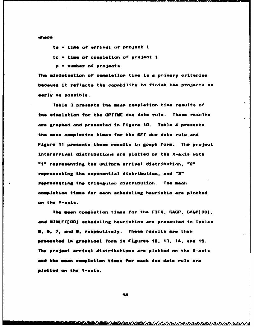
where

to - time of arrival of project I

to - time of completion of project I

p - number of projects

The minimization of completion time In a primary criterion

because It reflects the capability to finish the projects an

early as possible.

Table 3 presents the mean completion time results of

the simulation for the CPTIUE due date rule. These results

are graphed and presented In Figure 10. Table 4 presests

the men completion times for the SFT due date rule and

Figure 11 presents these results in graph form. The project

interarrival distributions are plotted on the X-axis with

"I representing the uniform arrival distribution, "2'

representing the exponential distribution, and "3'

representing the triangular distribution. The mean

ompletion times for each scheduling heuristic are plotted

on the V-axis.

The meon completion times for the FIFS, SASP, BASP[DDJ,

and NZNLFT[DOJ scheduling heuristic* are presensted In Tables

S, 6, 7, and 0, respectively. These results are then

presented In graphical form In Figures 12, 13, 14, and 1S.

The project arrival distributions are plotted on the X-axis

and %he mean completion times for each due date rule are

plotted en the I-axle.

so

The first observation to be made in that the GASP

scheduling heuristic mean completion time performance is

better then the other three heuristics for both due date

rules. In fact, the other three heuristics, FIFS, BASP[DD],

and MINLFTCDO], perform almost identically in each case.

Secondly, for all four heuristics, it Is apparent that the

mean completion times are sensitive to the difference in

project interarrival distributions. The results for the

uniform and triangular distributions are similar, but are

somewhat higher for the exponential interarrival

distribution. Also, it is apparent that there is

virtually no difference in mean completion times between the

two due date rules Investigated. Finally,.because all of

the lines in the graphs shown above remain parallel between

graphs it is assumed that there was no interaction effects

present for the mean completion time results. Only the

scheduling heuristic and arrival distribution main effects

are present in the man completion time results shown above.

A three-factor ANOVA was conducted for the above mean

completion time results and it was determined that there

is a significant difference in the mean completion times

between the "in factors of scheduling heuristic and the

arrival distribution, but not for the due date rule main

faster in this phase of the experiment. Also, all of the

two-factor and three-factor Interactions were notlig

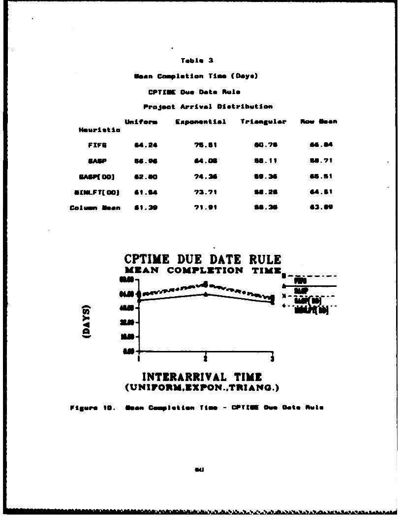
Table 3

Mean Completion Time (Days)

CPTIME Due Dats Rule

Project Arrival Distribution

HeuisicUniform Exponential Triangular PoW Oeaon

FIFU 64.24 75.51 60.76 66.64

SASP 54.96 ".D an6. 11 80.71

BASK 001 62.00 74.36 6.36 Wa.5

UINLFT[DDJ 61.54 73.71 56. 26 6.51

Column seen 61.36 71.91 56.26 63.66

CPTIME DUE DATE RULEMEAN COMPLETION TIME*---

INTIRARRIVAL TIMEC(UNIVOIRM.EXPON..TRtIANO.)

Fioure 10. Sean Caimpletison Tim - CPTw Owe Oaks Rule

SU

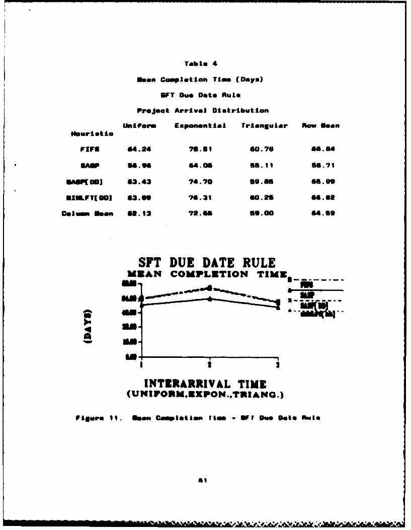
Table 4

Seen Completion Time (Days)

UFT Oue Oats Rule

Project Arrival Distribution

Uniform Exponential Triangular Row MeanHeuristic

FIF6 64.24 76.81 60.76 6.64

SAiP 6.6 64.06 n 6.11 8.7

oAoP(D 63.43 74.70 so. 66.00

8ZtLPT( 00 43." 76.31 60.26 6 .6

Column SaM 6. 13 72.6 "60.00 64.60

SFT DUE DATE RULEMEAN COMPLETION TIMZ

INTZRARRIVAL TIME( UN I PO RN. I8X PON..TR A NQ. )

Figueo 11t. Geo Completionl riml - WDue Date Ruk Ile

#51-

Tabl to

Mean Coimpletion Time (Days)

FIFE Vuheduling Heuristic

Project Arrival. Distribution

Uniform Exponential rriongula' Row MeanOwe Date Rule

CPT1W 624 76.51 60.76 66.64

GFT 64.24 751 60.76 66.54

Column often 6.24 75.61 60.76 66.64

FIFS HEURISTICME9AN COMPLETION TIME9

INTERARRIVAL TIME(UNIVPORM.EXPON..TXIANG.)

Figure 12. son. Completion Tim- FIF6 Heuristic

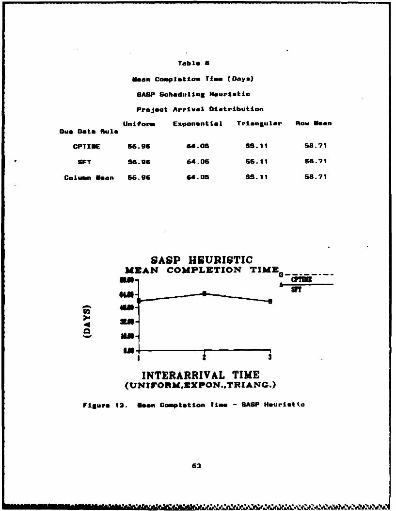
Table 6

Mean Completion Time (Days)

GASP Scheduling Heuristic

Project Arrival Distribution

Uniform Exponential Triangular Row Mean

Due Date Rule

CPTIME 56.96 64.05 55.11 583.71

OFT 56.96 64.05 55.11 58.71

Column Mean S6.96 64.05 55.11 58.71

19ASP HEURISTICMEAN COMPLETION TIMES-----

INTERARRIVAL TIME(UNrroRM.EXPON..TRIANG.)

Figure 13. Neon Completion rime - GASP Hourtautc

63

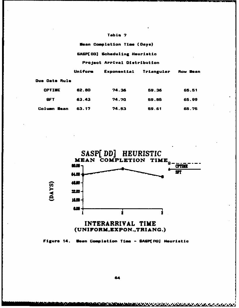
Table ?

Mean Completion Time (Days)

GAGPEDOJ Scheduling Heuristic

Project Arrival Distribution

Uniform Exponential Triangular Row Mean

Due Date Rule

CPTIUE 62.80 74.36 59.36 65.51

GFT 63.43 74.70 59.85 65.99

Column Mean 63.17 74.53 59.61 65.75

SASP( DD] HEURISTICMEAN COMPLETION TIME9 - - - - -

484

INTERARRIVAL TIME(UNIFORM.ZXPON..TRIANG.)

Figure 14. Een Completion Time - BASK[POJ Heuristic

64

Table B

Mean Completion Tim (Days)

MINLFT[DDJ Scheduling Heuristic

Project Arrival Distribution

DueDae RleUniform Exponential Triangular Row Mean

CIPTIME 61.54 73.71 56.28. 64.51

OFT 63.89 76.31 60.2S 66.81

Column Mean -62.71 75.01 59.27 65.61

MINLFT( DD] HEURISTICMEAN COMPLETION TIME0

*#APOM.E PO .. TWA-.

oil

Figure 15. Mean Completion Tim- MINLFT(O Heuristic

5

iLC

significant for mean completion times at the 0.05 family

level of significance (see Appendix A).

Multiple comparison tests were conducted to investigate

the significant differences in scheduling heuristic and

project arrival distribution and to identify which levels of

those factors were significantly different. Tukey,

Bonferroni, and Saheffe teats were conducted at the .05

level using the SAG software system for data analysis

(19). Significant differences were found at this level

which is very conservative. The results indicated

that only the GASP scheduling heuristic is significantly

different in mean completion time performance out of the

four heuristics tested. There were no significant

differences in performence attributable to the due date

assignment rule used, however, significant differences in

mean completion time wera found for each level of project

arrival distribution.

To summarize the analysis on mean completion time, it

was found that the GASP heuristic performs significantly

better than the FIFS, SASPIDUJ, and MINLFT[DOJ heuristics

which perform on the some level. Additionally, no

significent differences in mean completion time were found

attributable to the CPrziE or SFT due date rules. At the

.06 family level of significence, the meen completion times

were found to be significantly different for each of the

project arrival distributions Investigated. Finally, no

66

significant two-factor or threw-factor interaction effects

for mean completion time were found by this analysis.

Mean Delay Time . Nean delay time (or mean lateness)

Is a measure of the delay (bath positive and negative)

between the actual completion time and the estimated

completion time of a project (due date). It Is determined

as follows (5:69):

pE (to&. - dda)]/p()L-1

where

dds - due date of project I

t&- time of completion of project I

p - number of projects

Recall that In this experiment the effort was made to

achieve near zeo lateness In order to establish good duo

date compensation factors (k' values) for each combination

of due date rule, schedulng heuristic, and project arrival

distribution. Those due date compensation factors were

applied to the due date setting rules to Improve their

performance. The table of meon lateness values in presented

In Tables 9 and 10. They ore presented graphically in

Figures 16 and 17 acording to due date rule.

A three-factor ANUVA was performed to determine if

there were any significant differences In project mean

lateness. Me main footer or Interaction effects were found

in this oeariment at the 06 family level of significanie

Table 9

Sen Delay Tim (Days)

CPTINE Due Date Rule

Project Arrival Distribution

Uniform Exponential Triangular Raw Haan

Heuristic

FIFO 1.01 0.75 0.46 0.74

SASP 0.32 0.88 0.34 0.50

SAGP(001 -0.90 0.76 0.25 0.05

*IULFTEDO) 0.43 1.01 0.35 0.60

Column We.. 0.22 0.64 0.36 0.47

CPTIME DUE DATE RULEMEAN DELAY TIME

JA P---- ----

NEW

am x SA3INT RARRVAL TIM

(UNIO-.ZP-.TRA-.

Fiur 16 SoDeaTie C INDuOnRuIle~~

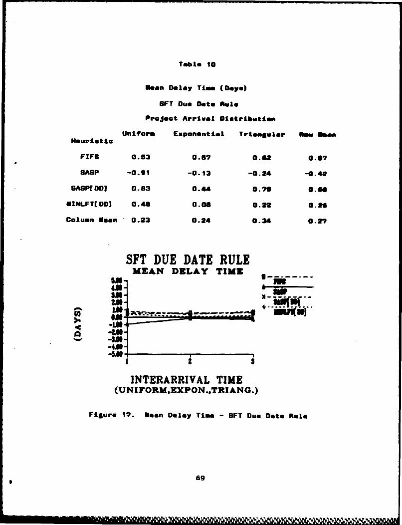
Table 10

Mean Delay Tim (Days)

OFT Due Doe Rule

Project Arrive Distribution

Uniform Exponential Trisagular Now go"Hour itle

FIFE 0.53 0.17 0.62 0.67

9A9P -0.91 -0.13 -0.24 -0.48

SASP[OD] 0.83 0.44 0. " 3. GM

MINLFTCDD] 0.48 0.06 0.22 a."L

Column lean 0.23 0.24 0.34 0.27

SFT DUE DATE RULEMEAN DELAY TIME

&A"

4JU!3-- --

LU,

-2.U-3m--4-40

INTERARRIVAL TIME(UNIFORM.EXPON..TRIANG.)

Figure 19. Mean Delay Time - EFT Due Date Rule

69

This snL06 a%"e h the ehelee of h W Las (see Tables I and

M) predmed due d*O*e Whih.f In oamee £ resulted L0e e

LS&OnMS Of OPrOVe1041 NOVO. #4soe 0&A. &his reslt ca 6e

oesteod due to te lateotamoi dootS of the sepe.' mut

afihf We to inhso neor so"s lotaee for al aeIheervot soee

ftyL"" 2ftma U1h5 iess mesre of

peorfesmeeso is weed to Prosid som ifteigt Lae the sOa"

of ths 1040000e distributioen. A low Otw"od deviatiLon of

14t0MOOe deomeeuoee thot amet of the pro jeets sees

obe to ott their due doto* while a high standard

dows~eno of Lateess 9ad10e600 thot meet projects will

edse their due doteso bp a ooiderabbe amount of ti~e.

The standard deviots of latoeess is determined as fellows

(6:74):

p pE ( to& -dde) 01Ap- 1)-1 C (tes-dds) Ip/( p- 1) ) 1.1 Ce)

where

dda - due dote of project I

to& - tie of completion of project I

p - number of projects

The standard deviation of lateness results are

presented according to due date rule In tabular fore In

Tables 11 end 12, end In graphical form In Figures 16 end

19. Likewise, the results are also presented according to

scheduling heuristic In tabular form In Tables 13, 14, 15,

70

sod 6I, end in graieDsl foer tn FIgures 20, 21, "1, and 23.

e4ewl bservationee Oda be made frem the data sed are

ouapertod by the theem-feeter MmVA:

I. The tuo due dote artented heurietiee (SAGI001 and

UZLFVMI) perform abeut the se but meeh better for the

OFT due date rule.

R. The SAMP eouristio performs eigniftoantly wores

then the ethors fe beth due date rules although the

pewfoemaeas iproves for to OFT due date rule.

3. rhe FIFO huretieto performs about the so as the

two due dote oriented houristics when used with the CPTIUE

due date rule. blewever, its performance improves remorkably

when used with the OFT due date rule.

4. In general, there to on Improvement in the standard

deviatte of lateness when the mre sophisticated SFT due

date rule is used.

S. The performance of il four heuristias, for both

due date rules, is significantly worse for the exponential

project arrival distribution while the performance is the

same for the uniform and triangular arrival distributions.

S. An interesting observation can be made with

respect to the FIFS/BFT combination. It appears as though

this combination of scheduling heuristic and due date

assignment rule is Insensitive to differences In the

project arrival distribution for the measure of standard

deviation of lateness. Also, the due date oriented

71

~i

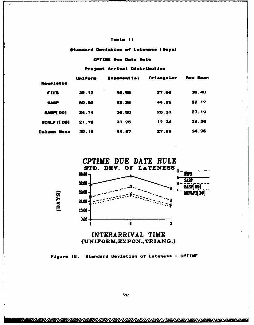
Tabl toI1

Stooard Deviatien of Lateness (Days)

CPric Own. Date Rule

Piejeet Arrival Diutributien

Uniform Iupmnntial rrionguier So0w sen

PIFU 22.12 ".96 27.06 36.40

§AGP 80.00 62.2 44.25 52.1?

BASPID03 24.74 36.60 20.33 27.19

*INLF1(DOJ 21.76 33.75 17.34 24.29

Column seen 32.16 4".a? 27.25 34.76

CPTIME DUE DATE RULESTD. DEV. OF LATENESS

b - S

.3W

INTERARRIVAL TIME(UNIFORMEXPON..TRIANG.)

Figure 16. Standard Deviation of Lateness - CPTIE

72

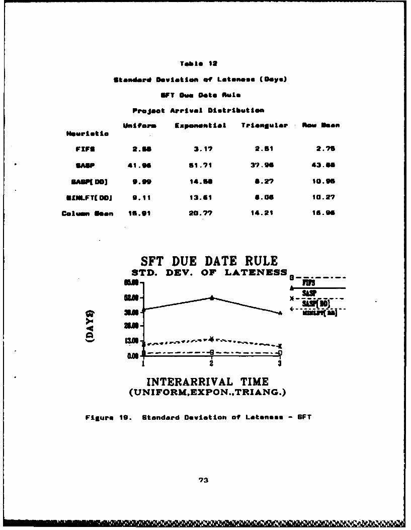
Table 12

Stlnard Deviation of Lateness (Days)

OFT Due Date Mule

Projeot Arrival Distribution

Uniform Expnmential Triangular Fow Son1"rltic

FIFU 2.68 3.17 2.61 2.75

SAUP 41.96 61.71 37. 9 43.66

AP(f W3 9.99 14.66 6.27 10.96

*ZNLFT(OOJ 9.11 13.61 8.06 10.27

Column Mean 15.91 20.77 14.21 16.96

SFT DUE DATE RULESTD. DEV. OF LATENESS

4

to0 ---- -- -. - - -

12 3

INTERARRIVAL TIME(UNIFORM,EXPON.,TRIANG.)

Figure 19. Standard Deviation of Lateness - UFT

73

Table 13

Stmoedrd Detion of Latenss (DOW*)

Ppejet Aarival *istributiem

unts"a *.apsoonat. friongulor 01. DeanDue Dean Rule

UPTIE W3.1 in.98 37.0 DO 3.4

OFT a."3 3.17 3.11 3.79

columnsion 17.21 25.07 14.60 13.06

FIFS HEURISTICSTD. DEY. OF LATENES*------

an-

4ur

INTERARRIVAL TIME(UNIFORM.EXPON..TRIANG.)

Figre 20. Standard Deviatfian of Lateness -FIFG

74

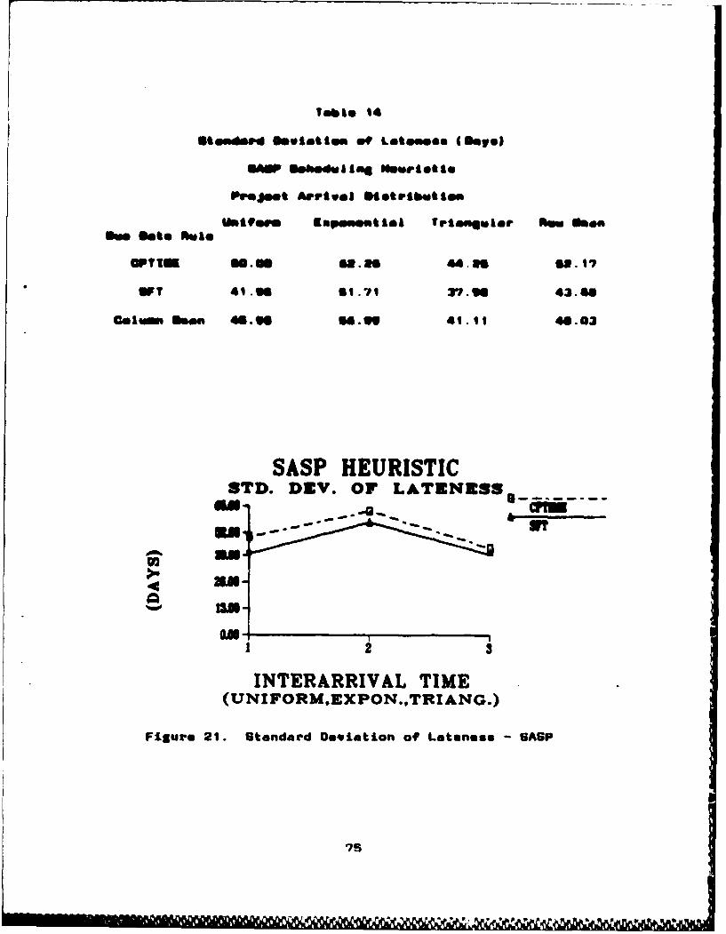
lete, 14

Stands"' Savtlm of Lateess (See

Puejme Artvei Distribtio

wMifew ampom.iea TrimmuI. Flow @**aDue make fta.

OPrim ftm Oas 6.- 817

WT 41."6 61.71 2.643. "

calo ine 46.m66 41.11 66.03

SASP HEURISTICSTD. DEY. OF LATENES 0 - - - - - -

JOE%

INTERARRIVAL TIME(UNIFORM.EXPON..TRIANG.)

Figure 21. Standard Deviation of Lateness S ASP

?5

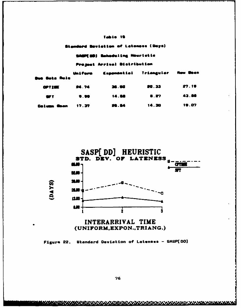
lab&* Is

Gteogoe S.etote of Latenes (Days)

GuwfwI safeduaarn fterisftlo

Puejot Apu'lvel *tDletution

Imafe"m Emponent Ao Trimnular flow s*"

OP3N 4.74 36.S. 33 27.19

WT 9.99 14.3 6 .37 43.3

column soon 17.7 35.54 14.20 16.07

SASP( DD] HEURISTICSTD. DEV. OF LATZNES*------

an-

183

INTERARRIVAL TIME(UNIFORM.EXPON..TRIANG.)

Figure 22. Standard Deviation of Latenss - GASPEDDJ

Table 16

Stesmiard Deviation of Lateness (Days)

*NLFTlDSJ Duhedualing Heuristic

Project Arrival Distribution

Uniform Exponential Triangular Flow Mean

"ae Date Rule

OPTIM a1."6 33. 75 17.34 24.29

0F .11 13.61 8.06 10.27

Colmn seen IS." 23.m 12.71 17.26

MfINLFT( DD] HEURISTICSTD. DEV. 0F LATENESS

a-

-U -

INTERARRIVAL TIME(UNIFORM.EXPON.,TRIANQ.)

Figure 23. Standard Deviation of Lateness - MINLFT[DOJ

77

scheduling heuristics, when woed with the UFT due date rule,

bee me lose ensitive to changes In the project errival

distribution, but not as much em the FZFS/GiFT coimbination.

7. There Is definitely ar eInteraction effects

present between the scheduling heuristic and due date

fators as well as ar eInteraction effects between the due

date rule and project arrival taoter*. This can be readily

seen In the graphs presented. Note that the parallelism for

these factors Is no longer present.

The three-factor ANOVA Indicates that there are

significant mein effects present at the 0.08 family level of

significance for~ all factors and there are significant

Interaction effects between heuristic and due date rule

combination@ and between due date rule and arrival

distribution combinations In the experiment. The results of

these statistical tests on the standard deviation of

lateness are provided In Appendix A.

Multiple comparison tests were conducted In order to

Identify which levels of the factors were significantly

different from one another. Tukay, Bonferroni, and Scheffe

tests were conducted at the 0.0073 level which provides a

family level of significance of 0.08. The results Indicated

that for the scheduling heuristic factor, the GASP heuristic

performs significantly worse than all of the other

heuristics tested. The due date rule factor tests Indicated

that the SFT due date rule provided significantly better

78

results In terms of the standard deviation of lateness

measure for all oases. This is especially true for the

FIFS/UFT ombination as illustrated in Figure 19. The ANOVA

slo indicates that all scheduling heuristic and due date

rule combinations perform significantly worse for the

exponential project arrival distribution level results.

In summeary, the standard deviation of lateness

results indicate that the SASP heuristic is a very poor

performer regardless of the due date rule and the FIFS/SFT

combination of scheduling heuristic and due date assignment

rule emerges as a remarkable performer. Most importantly,

the FIFG/9FT combination proved to be insensitive to the

project arrival distribution which is a desired result. The

due date oriented scheduling heuristics, when used with the

SFT due date rule, demonstrated a decrease in sensitivity to

project arrival distribution compared to the due date

oriented heuristics using the CPTIME due date rule. In

general, the exponential arrival distribution has a

significant impact on the standard deviation of lateness,

except for the FIFS/SFr heuristic and when the SFT due date

rule is used with due date oriented scheduling heuristics.

Mean Tardiness. Project mean tardiness is the average

amount of positive lateness for each project that has

exceeded its due date. It is determined as follows (6:104):

L (tardiness)Li/L (O

i-?

79

where

(tordiness)g = a if (to& - dd&) ip0

(tardiness) a - tog d., etheawiseM

L - total nuer of projects tardy

Project managers way be more eoncerned with bew lots,

on the average, they toad to omplete projects when tardy

then how often they miss due dote*. If tardiness to a were

Important factor, soon tardiness an provide a* fwdge'

factor for the project manager when promising due date* to

customers. The mean tardiness date to provided In tabular

form according to due date rule In Tables 17 and 10 and In

graphical form In Figures 24 and 2S. fables 19, 20, 21,

g2 end Figures 26, 27, 26, and 29 present the data

according to scheduling heuristic. 6ame general

observations can be ende from these results In tons of mean

tardiness performance:

I. The due date oriented scheduling heuristics

(SASPE DO] and *INLFTEDDJJ perform characteristically the

same for each due date rule and their performance is better

for the SFT due date rule than the CPTIUE due date rule.

2. The GASP heuristic performs poorly In terms of

project mean tardiness.

3. The FIFG heuristic performs remarkably well when

combined with the OFT due date rule.

so

- w 9;-",. ,

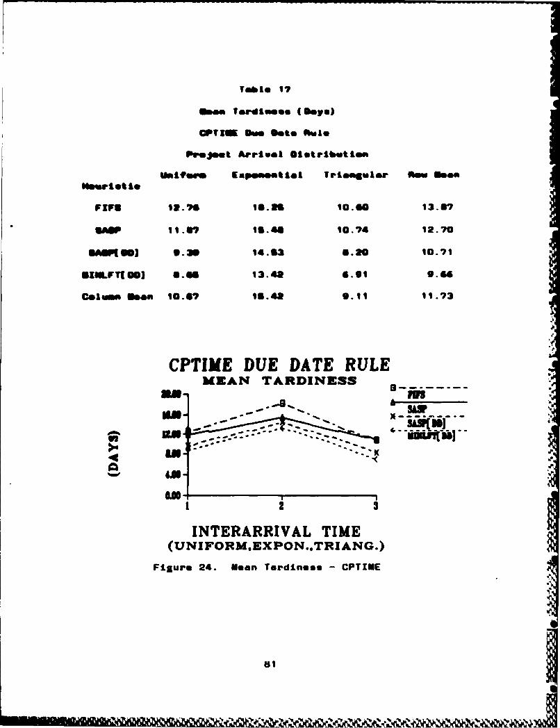
Table 17

Woom Tardiness (Dea)

OPT 1 Doe Seto Rue.

pu'ejeat Arrival Sistributties

waifae fiEaeseeti Trioewlor Now moos6"Wristie

FIFS 12.76 W6.S 10.60 13.07

SAWP 11.617 Is.46 10.74 12.70

APt ft) 9.39 14.63 G.&O 10.71

0*ILPF1 WS) 6.66 13.48 6.61 9.6"

Calm Eae 10.67 15.42 9.11 11.73

CPTIME DUE DATE RULEMEAN TARDINESS

SAW

4A4

'OI

2 3U

INTERARRIVAL TIME(UNJFORMEXPON..TRIANG.)

Figure 24. Mean Tardiness - CPTIUE

81

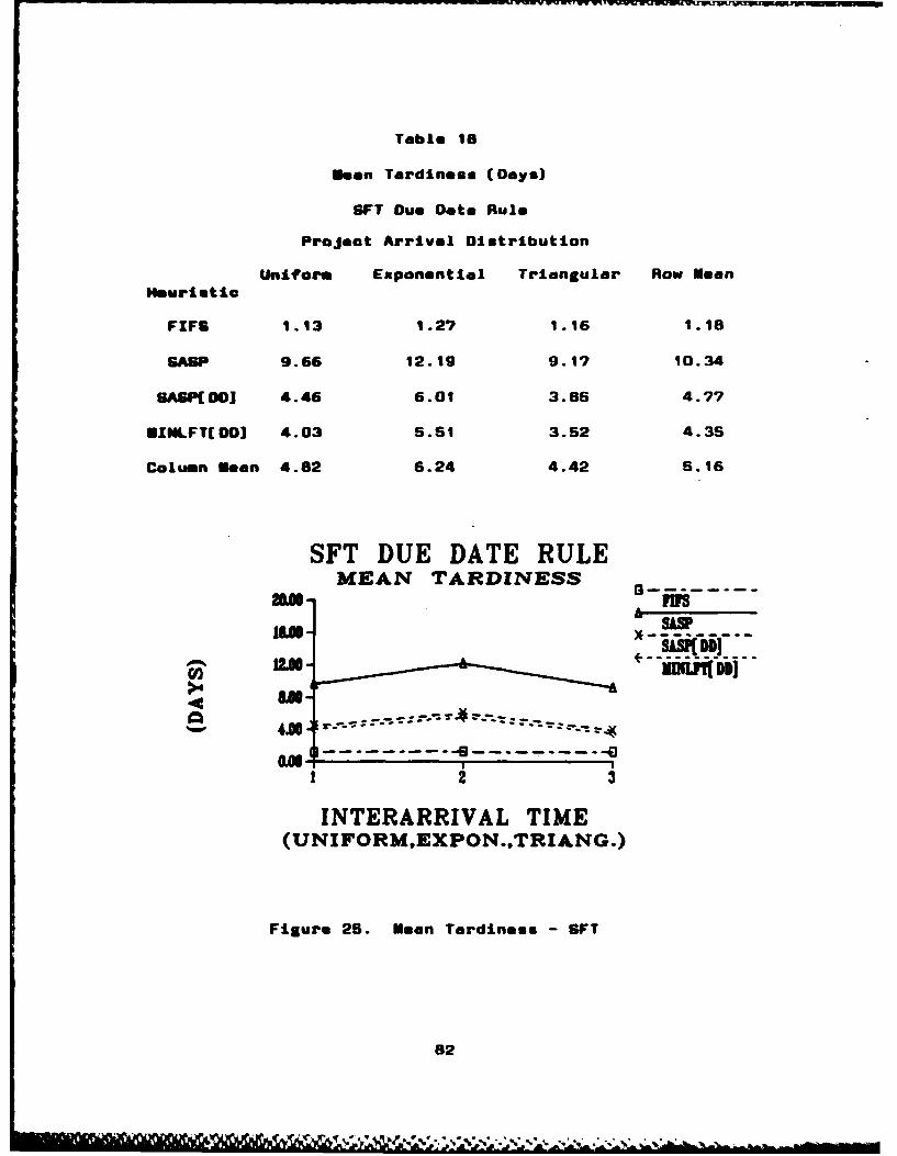
Table 18

man Tardiness (Days)

SFT Due Date, Rule

Project Arrival Distribution

Uniform Exponential Triangular Row MeanHeuristic

FIFU 1.13 1.27 1.16 1.18

GASP 9.66 12.19 9.1? 10.34

GASP(DDJ 4.46 6.01 3.85 4.77

*INLFT(DDJ 4.03 5.51 3.52 4.35

Column Mean 4.82 6.24 4.42 5.16

SFT DUE DATE RULE2LB-MEAN TARDINESS

SLV

16A -

INTERARRIVAL TIME(UNIFORM.EXPON.,TRIANG.)

Figure 25. Mean Tardiness - GFT

82

D-A167 057 AM EVALUATION OF PROJECT SCHEDULING TECHNIQUES IN A 2/2DYNNIIC ENVIRONNENT(U) AIR FORCE INST OF TECHWIGT-PRTTESSON AFD OH SCHOOL OF SYST. J 0 MARTIN M

UNCLASSIFIED SEP 8? RFIT/SN.LSY/07-19 F/G 12/4 M

I Khhhhhhhh

* ~ -4- 4 -

02

OR1~I~CIO

LMS

-. w.* *~ * * *Now=,

Table 19

Mean Tardiness (Days)

FIFO Scheduling Heuristic

Project Arrival Distribution

Uniform Exponential Triangular Row man

Due Dnto Rule

CPTIME 12.76 18.25 10.60 13.87

OFT 1.13 1.27 1.16 1.18

Column Mean 6.94 9.76 5.86 7.53

FIFS HEURISTICMEAN TARDINESS

V2

INTERARRIVAL TIME(UNIFORid.EXPON.,TRIANG.)

Figure 26. Mean Tardiness - FIFO Heuristic

03

TablIe 20

Mean Tardiness (Days)

GASP Scheduling Heuristic

Project Arrival Distribution

Uniform Exponential Triangular Row Mean

Due Date Rule

CPTIUE 11.87 15.48 10.74 12.70

GFT 9.66 12.19 9.17 10.34

Column Mean 10.77 13.83 9.95 11.52

SASP HEURISTICMEAN TARDINESS

4A

INTERARRIVAL TIME(UNIFORM.EXPON..TRIANG.)

Figure 27. Mean Tardiness -GASP Heuristic

84

Table 21

Mean Tardiness (Days)

SAGPf DO) Scheduling Heuristic

Project Arrival Distribution

Uniform Exponential Triangular Row Men

Due Date Rule

CPTIUE 9.39 14.83 8.20 10.71

6FT 4.46 6.01 3.65 4.7?

Column Mean 6.92 10.2? 6.02 7.74

SASP( DD] HEURISTICMEAN TARDINESS

UNIFOU-----------NG

FiueVa enTadns - BAPrHersi

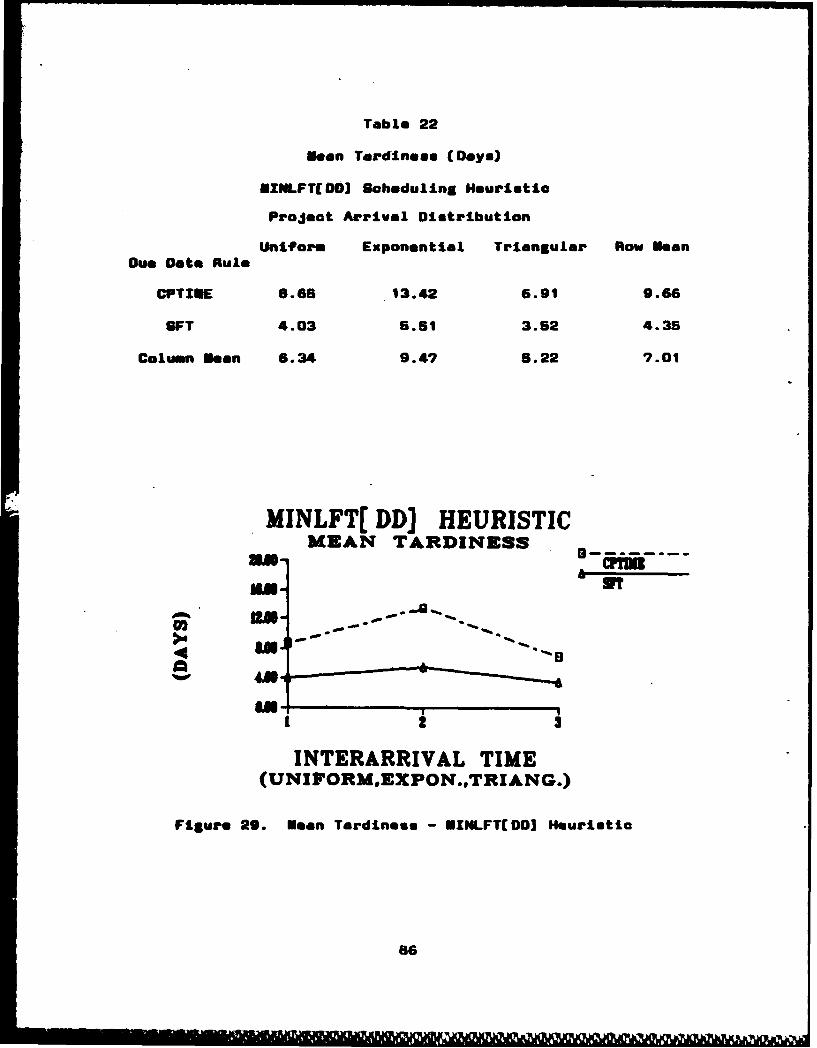
Table 22

Mean Tardiness (Days)

UZNLFT[DDJ Scheduling Heuristic

Project Arrival Distribution

Uniform Exponential Triangular Row Mean

Due Date Rule

CPTIUE 8.68 13.42 6.91 9.66

9FT 4.03 8.51 3.52 4.35

Column man 6.34 9.47 5.22 7.01

MJNLFT( DD] HEURISTICMEAN TARDINESS

0 -- -

NO 45t

INTERARRIVAL TIME(UNIVORWeEXPON.eTRIANG.)

Figure 29. Mean Tardiness - *INLFTCDDJ Heuristic

836

4. In general, the mean tardiness performance improves

across the board when the OFT due date rule is combined with

any of the scheduling heuristics tested In this experiment.

S. Again, the mean tardiness results from the

exponential arrival distribution tend to be worse than the

other two distributions investigated.

These observations are supported by the three-factor

ANOVA. Significant main effects for all three factors

(heuristic, due date rule, and arrival distribution).

Significant two-factor interaction effects were found for

the scheduling heuristic and due date rule factor

combinations as well as for the due date rule and arrival

distribution factor combinations. No other interaction

effects were found to be significant in this portion of the

experiment.

Eultiple comparison tests were conducted at the 0.0073

level to provide a family level of significance of 0.05 for

the seven tests. Tukey, Bonferroni, and Schsffe test were

conducted at the .05 family level of significance. The

results show that the BASP scheduling heuristic mean

tardiness performance is significantly worse then the

other three heuristics. There is clearly a significant

difference between both of the due date rules end the

exponential project arrival distribution accounts for the

differences in man tardiness. The ANOVA procedure and

87

L

statistical tests for mean tardiness can be found In

Appendix A.

In sumeary, the mean tardiness results indicate that

the ombination of FIFB scheduling heuristic and SFT due

date rule Is clearly the best performer while the

FIFS/CPTIME combination is the poorest. Most importantly,

the FIFO/SFT combination seems to be insensitive to

differences in project arrival distribution. The due date

oriented heuristics used with the 9FT due date rule also

demonstrated a dearease in sensitivity to the different

arrival distributions. This insensitivity is a desired

result because one would not have to be concerned about the

potential impact on mean tardiness if the arrival

distribution is unknown.

Average Resource Utilization Rate. This research

effort did not investigate thoroughly the behavior of the

resource utilization rate during the experiment other than

to make some general observations to ensure that the overall

resource utilization rate was approximately 85 per cent.

Upon completion of the simulation of 2000 days per

simulation run it was found that the average resource

utilization rate was approximately 85 per cent for all three

types of project arrival distribution. However, samples of

the average resource utilization rate during each simulation

run revealed some interesting behavior. The variation in

the resource utilization rate appears to be very small for

B

the uniform project arrival distribution runs. In other

words, the project load in the system tends to be fairly

constant during the 2000 days of simulation time. Likewise,

the triangular project arrival results revealed a small, but

somewhat larger then the uniform distribution, variation In

the average resource utilization rate during each run. The

interesting observation occurred during the exponential

project arrival distribution runs. The project interarrival

times tend to be very smell and very large at times, ausing

the project load in the system to vary during the simulation

and, therefore, the average resource utilization rate varies

considerably compared to the other project arrival

distribution runs. When the project interarrival time is

small the project load in the system is. high and therefore

the resource utilization rate Is high. On the other hand,

when the time between project arrivals is long the system

project load is law and consequently the resource

utilization rate is low. In the long run, the average

resource utilization rate for the exponential arrival

distribution is still approximately 6 per cent.

Suery of the Results

The purpose of this experiment was to produce data

from the simulation of the dynamic, multi-project,

constrained resources scheduling environment and analyze the

results to search for answers to the research questions

posed in Chapter 1. This experiment was an extension to

89

111009MMU

previous research conduated on the performance of scheduling

heuristios and due data assignment rules in a dynamic,

project scheduling environment. The objective was to

interject another factor into the previous experiments

performed, specifically, different types of project arrival

distributions, and to analyze the impact on the performance

of scheduling heuristics, due date assignment rules, and

combinations of scheduling heuristic and due date rule.

In order to address the research questions posed in

Chapter 1, the results have been grouped according to

project arrival distribution for each of the performance

parameters and presented below. The date is presented below

in both tabular and graphical format in order to clearly

present the differences in each performance measurement due

to differences in project arrival distribution.

The results of this three-factor, full factorial

experiment indicate that the performance of scheduling

heuristics, due date rules, and combinations thereof,

were similar to the two-factor experiments conducted earlier

by others (6). In other words, no new surprises were

discovered for the scheduling heuristic factor or the due

date rule factor. The OFT due date rule provides

significantly better performance on all due date measures

without any penalty in minimizing mean completion times (see

figures 30-36). However, it was discovered that the new

factor, project arrival distribution, impacts the ability of

90

TablIe 23

Mean Completion Time (Days)

Uniform Project Arrival Distribution

Duo Data Rule

CPTXNE SFT Row NeonHeuristic

0FF 64.24 64.24 64.24

* ASP 96.96 96.96 56.96

BSP[DDJ 62.80 63.43 63.12

*INLFTEDDJ 61.S4 63.89 62.71

Column Moon 61.39 62.13 61.76

UNIFORM ARRIVAL TIMEMEAN COMPLETION TIME

48A (-----------

UWLDD

U) UFan-D

DUE DATE RULE

Figure 30. Mean Completion TimeUniform Arrival Distribution

91

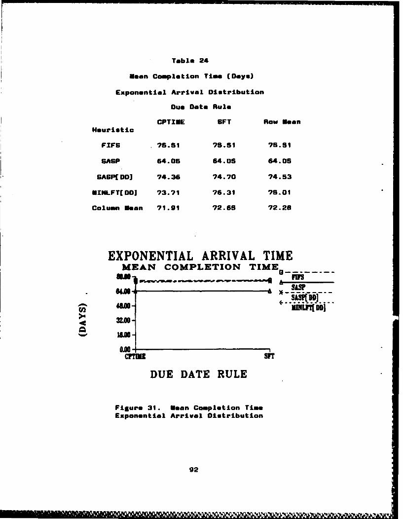
Table 24

Mean Completion Time (Days)

Exponential Arrival Distribution

Due Date Rule

CPTIUE SFT Row Mean

Heuristic

FIFS 75.81 75.51 75.51

SASP 64.05 64.05 64.05

SAGP[DD3 74.36 74.70 74.53

UINLFT(DDJ 73.71 76.31 75.01

Column Mean 71.91 72.65 72.21

EXPONENTIAL ARRIVAL TIMEMEAN COMPLETION TIME9

Ion

4400

%mow,

dYNE SIT

DUE DATE RULE

Figure 31. Mean Completion TimeExponential Arrival Distribution

92

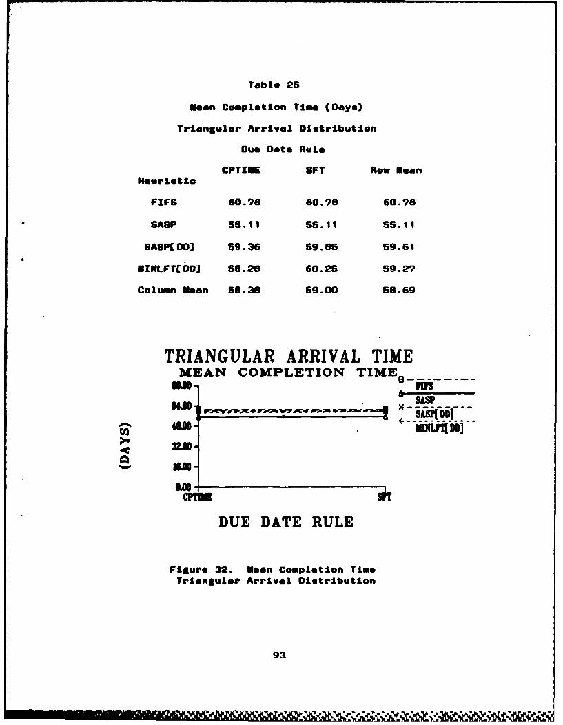
Table 25

Mean Completion Time (Days)

Triangular Arrival Distribution

Due Date Rule

Huitc CPTIUE OFT Row Mean

FIFO 60.78 60.70 60.78

GASP 55.11 65.11 55.11

BAGP[DDJ 59.36 89.85 59.61

HINLFTEDDJ 58.28 60.25 59.27

Column Mean 6.38 59.00 58.69

TRIANGULAR ARRIVAL TIMEMEAN COMPLETION TIMES-----

HAS

4 32..

IA

DUE DATE RULE

Figure 32. Sean Completion TimeTriangular Arrival Distribution

93

Table 26

Standard Deviation of Lateness (Days)

Uniform Arrival Distribution

Due Date Rule

CPTIUE SFT Row Mean

Heuristic

FIFS 32.12 2.58 17.35

GASP 50.00 41.96 4S.98

SASP[DDJ 24.74 9.99 17.3?

UINLFTCDDJ 21.78 9.11 15.45

Column Mean 32.16 15.91 24.04

UNIFORM ARRIVAL TIMESTD. DEV. OF LATENESS

Sir?56A -SXSP DDJ ---

14.0

3"T

DUE DATE RULE

Figure 33. Standard Daviatian of LatenessUniform Arrival Distribution

94

Table 27

Standard Deviation of Lateness (Days)

Exponential Arrival Distribution

Due Date Rule

CPTIUE OFT Row MeanHeuristic

FIFG 46.98 3.17 25.0?

GASP 62.26 81.71 56.99

GAGPEDDJ 36.50 14.58 25.54

*ZNLFT[DDJ 33.76 13.61 23.68

Column Mean 44.8? 20.?? 32.82

EXPONENTIAL ARRIVAL TIMESTD. DEV. OF LATENESS

rn 4196- ~. uILMrDD]

14.80

CPYIN 3"

DUE DATE RULE

Figure 34. StanaSard Deviation of LatenessExponential Arrival Distribution

95

' NA

Table 25

Standard Deviation of Lateness (Days)

Triangular Arrival Distribution

Due Date Rule

CPTIUE OFT Row BeenHeuristia

FIFO 27.08 2.51 14.80

amp 4425 37.96 41.11

SASPLODI 20.33 8.27 14.30

*IULFT[DDJ 17.34 8.06 12.71

Column Nean 27.25 14.21 20.73

TRIANGULAR ARRIVAL TIMESTD. DEV. OF LATENESS*----

71113

IAIT

DUE DATE RULE

Figure 36. Standard Deviation of LatenessTriangular Arrival Distribution

ge

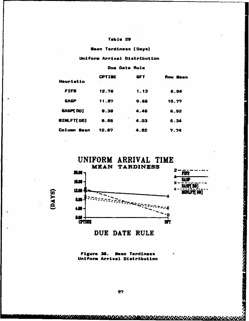
Table 29

Mean Tardiness (Days)

Uniform Arrival Distribution

Due Date Rule

CPTIUE OFT Row MeanHeuristic

FIFO 12.76 1.13 6.94

BASP 11.87 9.66 10.77

BSP[DDI 9.39 4.46 6.92

*IULFTCDDJ 8.66 4.03 6.34

Column Mean 10.67 4.62 7.74

UNIFORM ARRIVAL TIMEMEAN TARDINESS

SIP

ca

DUE DATE RULE

Figure 36. Mean TardinessUniform Arrival Distribution

97

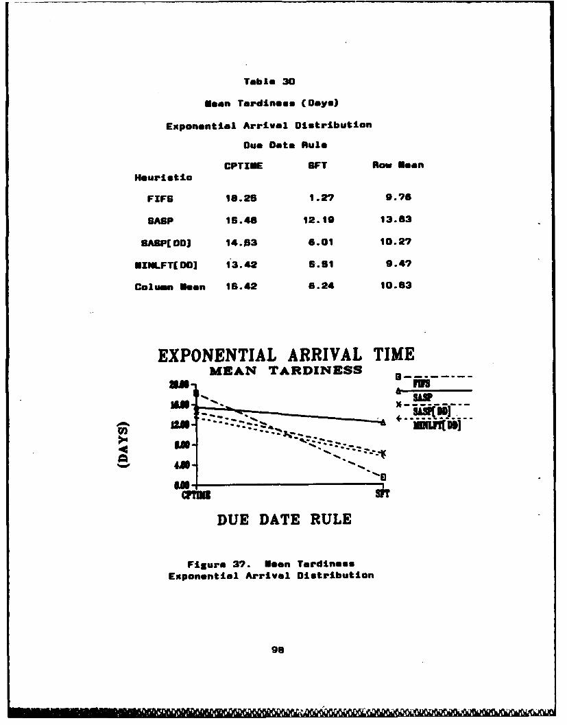
Table 30

Sean Tardiness (Days)

Exsponential Arrival Distribution

Due Date Rule

CPTIME OFT Row Mean

Heuristic

FIFO 16.28 1.27 9.76

9ASP 18.46 12.19 13.63

BABP[ODD 14.103 6.01 10.27

*INLFT(D 13.42 8.81 9.4?

Column Meon 18.42 6.24 10.83

EXPONENTIAL ARRIVAL TIME3WMEAN TARDINESS

16AN

1A-

4 A-

4-

DUE DATE RULE

Figure 3?. Mean TardinessExponential Arrival Distribution

963

Table 31

Keen Tardiness (Days)

Traengular Arival Distribution

Due Dote Rule

CPTXUE SIFT Row manHeuristic

FIFG 10.60 1.16 5.66

SASP 10.?4 9.17 9.96

BASPCD 6.20 3.05 6.02

*IMLFT[DDJ 6.91 3.9 8.22

Column lean 9.11 4.42 6.77

TRIANGULAR ARRIVAL TIMEMEAN TARDINES

am S m

Figur 38 Ma Trins

TraglrArvlDsrbto

US - -- ~: 99

due date assignment rules and scheduling heuristics to met

due dates. Therefore, the reminder of this discussion will

focus on the reseerch questions posed in Chapter 1.

Research Question 1. Are scheduling heuristics,

investigated in previous research, Impacted by whether new

projects arrive according to a uniform, exponential, or

triangular distribution?

This question is answered In terms of two major

performance criteria: ability to minimize the mean

completion time of projects and ability to met established

due dates.

If man completion time is the important factor then

the results show that all of the heuristics tested were

found to be sensitive to each of the different project

arrival distributions. Figures 10 and 11 illustrate

the differences in man completion time for each project

arrival distribution. The three-factor ANOVA revealed a

significant difference in mean completion times existed and

the multiple comparison tests indicated that all three

project arrival distribution mean completion times were

significantly different from one another. The average men

completion times for each scheduling heuristic are the

column mean values shown in Tables 3 and 4.

The SAIP heuristic is the best performing heuristic in

terms of mean completion tim while the other three

heuristics perform equally well but worse than the 9ASP

100

heuristic. If the 9ABP heuristic is chosen based on its

man completion tIm performince then one needs to be aware

that it's exceptional performance Is due to Its ability to

get small projects done very quickly, at the expense of long

projects which take longer than normally expected.

The ability of scheduling heuristics to meet

established due dates is measured in terms of standard

deviation of lateness and man tardiness. The standard

deviation of lateness measures how close to the due date

projects are completed. Mean tardiness measures the average

tardiness (positive lateness) of a project when It Is tardy.

The performance of the heuristics relative to these measures

is the sam and will be discussed together.

The SASP heuristic performs poorly on these due date

performance measures. With regard to both standard

deviation of lateness and mean tardiness it performed

significantly worse then the other three heuristics tested,

SASP(DDI, UINLFT[OO], end FIFO (see Tables 11, 12, 17 and 18

and Figures 16, 19, 24 and 25). These letter three

heuristics performed equally well on both due date measures.

The performance of all four heuristics deteriorates when the

projects arrive according to an exponential distribution

relative to their performance when projects arrive according

to a uniform or triangular distribution. It must be noted

that, although the absolute performnce of the heuristics

changes depending on the arrival distribution, the relative

101

performanoe of the heuristics is unchanged and similar to

that found earlier (6, 6).

In suary, the answer to this research question is

that the heuristics do perform differently, in an absolute

sense, depending on the arrival distribution of new

projects. However, in a relative sense the heuristics

perform the same; that is, SAP does better in minimizing

man completion time and worse at meting due dates than the

other three heuristics tested (FIFe, Alp[DO], and

MINLFTDD]), regardless of the arrival distribution. This

finding extends the generalizability of the research cited

earlier (5, 6).

Research Question 2. Are due date setting rules,

investigated in previous research, Impacted by whether new

projects arrive according to a uniform, exponential, or

triangular distribution?

Recall that the due date for each project is set when

it arrives to the system and is established by either the

CPTIME or 9FT due date assignment rule. Figures 30-38

illustrate the comparison of CPTIEE and 9FT due date

assignment rules and their impact on the various performance

measures observed in this experiment. Again, this question

will be answered in terms of two major performance criteria:

ability to minimize the man completion time of projects and

ability to met established due dates.

102

With regard to mean completion time, there Is vary

little difference in man completion time attributable to

differences in due date rules (see Figures 30-32). However,

man oompletion time performance is sensitive to the project

arrival distribution and scheduling heuristic used.

With regard to due date performance it is obvious that

the OFT due date assignment rule does a much better job at

setting due dates, regardless of the project arrival

distribution, compared to the CPTIUE rule (see Figures 33-

36). The standard deviation of lateness and mean tardiness

is sensitive to the project arrival distribution and

scheduling heuristic used when due dates are set according

to the CPTIUE rule. In general, this sensitivity diminishes

when the OFT due date assignment rule Is used.

In summary, the answer to this research question Is

that due date assignment rules do perform differently , In

an absolute sense, depending on the arrival distribution of

new projects. However, In a relative sense the due date

setting rules perform the same: that is, SFT is a much

better method of setting due dates when meeting due dates

Is Important. In terms of minimizing man completion time,

the CPTINE and OFT due date assignment rules perform equally

well. This finding extends the generalizability of the

research cited earlier (6, 6).

103

Research Question 3. Are any combination of

scheduling heuristic and due date setting rule, Investigated

earlier, Impacted by whether new projects arrive according

to a uniform, exponential, or triangular distribution?

With regard to mean completion tie, there was

virtually no difference attributable to a specific

combination. Although 9AGP outperformed the other

heuristics on this measure, Its performance was identical

for the BA9P/CPTIME combination and the GASP/SFT

combination. Likewise, the other three heuristics when

combined with a due date setting rule resulted in virtually

the same performance regardless of which due date setting

rule was used.

This was not the case with regard to the due date

performance criteria, standard deviation of Lateness and

mean tardiness. As noted in the answer to research question

2, the OFT due date setting rule outperformed the CPTIME due

date setting rule. When the OFT rule is used in combination

with any heuristic, the combination outperformed, on both

due date measures, the CPTIME combination with that same

heuristic.

The most interesting observation during this experiment

was the outstanding performance of one combination,

FPFS/SFT, on the due date criteria. This combination

outperformed all other combinations on both due date

measures. Additionally, its due date performance remained

104

10a

the beast regardless of the arrival distribution of new

projects. It appears reasonably insensitive to the arrival

distribution. This result extends the generalizability of

the research cited earlir (S, 6).

This chapter provided the detailed results of the

experiment and addressed the three research questions posed

earlier in Chapter 1. These results will be summarized In

Chapter 4 and some Insight to the significance of these

findings, practical Implications of these results, and

suggestions for future research will be provided.

105

IV. Conclusions and Recommandations

This chapter summarizes the results of the simulation

experiment. The results indicate that scheduling

heuristics, due date rules, and combinations thereof are

generally sensitive, in an absolute sense, to whether

projects arrive according to uniform, exponential, or

triangular distributions. They also confirm that the

relative performance of the tested scheduling heuristics,

due date assignment rules, and combinations thereof, Is the

same regardless of the project arrival distribution.

Additionally, one particular combination, the FIFS

scheduling heuristic and SFT due date assignment rule,

proved to be insensitive even In an absolute sense to the

different arrival distributions tested. The significance of

these findings, a discussion of the practical implications

of these findings, and recommendations for future research

are addressed below.

Significance of the Findings. Although management can

control the method for setting due dates and scheduling

resources to activities to meet theme due dates, it cannot

easily control the arrival distribution of new projects.

Performance of several heuristics and due date setting rules

wis previously determined for projects arriving uniformly.

It Is important to know If these findings hold for other

arrival distributions and, if not, which heuristics and due

date rules perform better in different environments.

106

In almost every case it was found that the absolute

performance of scheduling heuristics and/or due date

assignment rules are most sensitive to the exponential

project arrival distribution. The performance with regard

to mean completion time was significantly different for each

arrival distribution, and worst in the exponential arrival

distribution environment. The performance of the scheduling

heuristics and due date setting rules on the due date

criteria, standard deviation of lateness and mean tardiness,

was found to be significantly different for the exponential

arrival distribution.

The differences in relative performance attributable to

either the scheduling heuristic factor or the due date

assignment rule factor of this experiment were basically the

same results observed previously (5). GASP performs well on

the criterion of mean completion time but poorly on the due

date oriented measures. And, in general, the other three

heuristics tested, SASP[DDJ, MXNLFT[DD], and FIFS, perform

equally well. The analysis indicated some interaction

between the due date rule factor and the arrival

distribution factor for the standard deviation of lateness

and mean tardiness results. In general, the GFT due date

assignment rule performed significantly better than the

CPTIUE rule even in the difficult exponential arrival

distribution environment. The GFT due date rule

seems to adjust well to the project arrival distributions.

10?

h

And, although the CPTIME due date rule is much simpler to

implement than the SFT due date rule, it was found to be

more sensitive to different project arrival distributions.

The SFT due date rule determines the early activity

start times of each new project based on resource

availability at that time. If the system is relatively

empty, the SFT rule will assign a shorter due date and when

the system is full it will assign a longer due date. The

SFT due date rule compensates for fluctuations in the

project load of the system. The triangular arrival

distribution introduced some fluctuations in resource

utilization compared to the uniform arrival distribution.

The exponential arrival distribution caused significant

changes in the system project load and apparently the SFT

due date rule compensates for this very well, especially

when combined with the FIFS heuristic.

The important discovery of this research was that the

FIF6/SFT combination provided outstanding results regardless

of the project arrival distribution. It was found that this

particular combination is insensitive to whether new

projects arrive according to the uniform, exponential, or

triangular distribution. The FIFG/GFT combination was found

to be the leading performer in previous research and it

remains so in this research.

108

The conclusion to made that the FIFS/GFr combination

performs the best for two reasons:

1. The OFT due date rule Is scheduling heuristic

oriented, meaning It provides very good estimates of the

project completion time which tends to be met by the FIFG

heuristic (8:193).

2. The FIFO heuristic Ignores due dates and therefore

is not as *nervousa as the due date oriented heuristics

(5:193).

The major significance of these findings is that

although there is sensitivity to project arrival

distributions, the relative performance of the tested

scheduling heuristics, due date assignment rules, and

combinations of scheduling heuristic and due date

assignment rules is unchanged regardless of the project

arrival distribution. Because the three distributions

examined (uniform, exponential, and triangular) represent

the most likely to occur, this research has ruled out the

factor of project arrival distribution in the dynamic,

multi-project, constrained resources scheduling problem.

The major contributions of this research were: 1)

identifying the specific impact of different project arrival

distributions on the performance of scheduling heuristics,

due date assignment rules, and combinations thereof; 2)

Identifying that no significant interactions between the

project arrival distribution, scheduling heuristic, or due

109

date assignment rule were found to drastically change the

behavior of scheduling heuristics or due date rules

investigated previously; 3) the discovery that the SFT rule

decreases the sensitivity to changes in project arrival

distribution; and 4) the FIF9/SFT combination performanoe

proved to be insensitive to whether new projects arrived

uniformly, exponentially, or approximately normal

(triangular distribution).

Practical Implications of the Results. This research

has addressed the issue of what impact differences in

project arrival distribution may have on procedures for

setting due dates and scheduling project activities to meet

those due dates in a dynamic, multi-project, constrained

multiple resource, environment. In general it was found

that different project arrival distributions do affect the

performance of scheduling heuristics and due date setting

rules in an absolute sense, but not in a relative sense.

Because of this, the project manager does not really need to

be concerned about the arrival distribution of new projects

because the relative performance of the tested heuristics

and due date assignment rules is the sam.

The best results are obtained when the Boheduled Finish

Time (BFT) due date setting rule is applied. Not only does

it provide the most accurate due dates, it provides

significantly better results when used with any scheduling

heuristic than the other due date setting rules, and it is

110

virtually not affected at all by differences in project

arrival distribution. Every project manager probably dreams

of such a procedure being available, however there is a

price to pay for the OFT due date assignment rule. The OFT

due date setting rule requires a finite scheduling system,

the ourrent status of all projects in the system, and a

historical data base to establish the due date compensation

factor ("k" value). Not all project managers could

implement this procedure due to the computer

hardware/software requirements, financial constraints,

project duration uncertainty, resource constraints, etc..

If they could use the SFT rule to smet the due date of the

arriving project, they would be wise to use the very simple

First-In-Firet-Berved (FIFO) scheduling heuristic to

allocate resources to the project.

An alternative to project managers would be to choose

the easier to Implement CPT1ME due date rule. If this is

the case then the manager would want to choose one of the

due date oriented heuristics to schedule the activities.

The GASP[DD and UINLFT[DD] produce similar results using

the CPTIUE due dote rule. The CPTIME due date setting rule

ignores the current project load when estimating activity

completion times and therefore lacks the "self-compensating "

feature of the OFT due date assignment rule.

Recall that the goals of the project manager are to

first of all determine reasonable due dates for each project

111

in order to make a promised completion date to the customer

and then schedule those projects accordingly so that due

dates are met on time. This research has determined that

the relative performance of the tested scheduling heuristics

and due date setting rules is unaffected by the project

arrival distribution. For the project manager, this

confirms that certain scheduling heuristics, due date

assignment rules, and combinations thereof will perform

better than others regardless of the project arrival

distribution. Therefore, the alternatives to management are

1) accept the decrease in performance capability for the

easier to implement CPTIME due date assignment rule used

with the due date oriented heuristics; or 2) make the

necessary commitments and investments to implement at least

one of these heuristics combined with the SFT due date

assignment procedure or better yet; 3) implement the

FIF9/9FT combination for assured performance.

Recommendations for Future Research. Relatively little

research has been devoted to the study *of the dynamic,

multi-project, constrained resources scheduling problem

which many project managers face ever day in reality. The

advantage of due date setting rules and scheduling

heuristics is they are good enough procedures for planning

and control purposes in light of the difficulties and

complexities involved with uncertainties in activity

durations, resource constraints, dynamic project arrivals,

112

and so on. Therefore, this area of project management

remains wide open for new research to make the project

manager's task of scheduling and meting due dates much

simpler. The author provides these suggestions for possible

future research:

1. Evaluate other due date setting rules and

scheduling heuristics with the uniform, exponential, and

triangular project arrival distributions.

2. Explore other project environmental factors such as

different levels of resources, stochastic activity

durations, dynamic resource availabilities, etc., and

conduct a multi-factor experiment to investigate their

impact on setting due dates and using scheduling heuristics

to meet those due dates.

These and many other areas of future research could add

to the robustness of scheduling heuristics and due date

assignment rules already available to today's project

managers. The goal of this and any other research in this

area should be to provide good tools to project managers so

that they can make better estimates of project completion

times and deliver the product or service on time, as much as

possible, to the customer.

113

Appendix A: Three Factor ANOVA Results

Appendix A contains the three-factor analysis of

variance results and presents the ANOVA table and

statistical test procedures used to test for main effects,

two-factor interaction effecats and three-factor interaction

effects for each of the following performance parameters:

1. Mean completion time.

2. Mean delay time.

3. Standard Deviation of Lateness.

4. Mean Tardiness.

For each parameter listed above a copy of the GAG

program is provided and the ANOVA statistical test procedure

Is shown. The multiple comparison tests are not shown but

are readily available by executing the GAG programs included

in this Appendix.

Mean Completion Time

The SAG program code developed for the mean completion

time performance parameter is shown in Figure 39. The

output of this source code is an ANOVA table, main and

interaction effects tests, and multiple comparison tests

(Tukey, Sonferroni, and Scheffe). Table 32 shows the ANOVA

table results for the mean completion time performance

parameter.

The seven statistical tests for factor effects and

interaction effects are shown below. The nomenclature for

these tests follow that used by Neter and Wasserman (14).

114

~B

otios Iinogigo.79 posouize-66;1* THI1S PROGRAM WILL PROVIO9 A THREE FACTOR FULL FACTORIALANALYSIS OF VARIANSCE USING PROC ANOVA ON THE PERFORMANCPARAMETER ... PROJEC MAN COMPLCTION TIME.

date moenoomp;do softed-1 to 4;

do dd-1 to 2;do arrtwel to 3;

do oervt to a;input y SO;output;and;

and;end;

end;cards;69.47 64.13 60.47 87.81 64.39 59.73 19.26 66.555.8 72.72 68.11 60.26 75.79 67.92 76.39 92.2664.24 59.66 17.99 63.58 41.14 87.33 56S.25 84.0589.5? 84.f3 60.47 67.61 84.39 59.73 19.21 68.5

.8.672.72 8.11 60.26 76.79 67.62 76.39 92.2664.24 60.66 17.99 83.14 61.14 57.33 16.29 64.0916.10 56.94 11.26 19.09 36.76 95.72 16.66 6.10116.03 83.64 56.35 6.66 65.95 61.56 65.36 73.636.21 84.06 64.39 S8.48 64.58 53.62 14.40 66.8356.10 56.94 15.26 19.03 36.78515.73 66.68 56.1016.03 82.64 66.35 66.66 85.91 61.8 85.38 73.6368.2f 54.06 64.30 58.48 $4.66 13.52 14.40 $6.6364.07 81.56 59.01 68.35 62.96 50.98 66.66 68.16665 71.62 64.20 75.11 76.36 69.36 764 67.661.62 57.97 8.67 61.58 69.60 66.91 68.43 82.0167.81 62.20 19.66 86.71 64.84 19.6 80.20 66.26$6.64.11.92 66.76 79.74 79.43 70.95 76.45 68.7661.86 59.22 57.77 63.00 60.65 16.33 16.21 61.5264.96 61.71 16.42 64.57 61.91 17.96 1906 63.4884.99 71.05 85.62 76.62 1.72 66.33 77.03 67.0060.64 17.35 65.62 61.26 56.62 15.26 17.26 19.6066.43 63.10 61.32 67.04 63.99 59.36 60.56 66.668.07 72.34 69.21 60.77 60.81 89.61 79.84 99.6A

62.10 19.18 17.62 64.08 61.30 58.00 9.26 62.12prod. means;

title 'GROUP MEANS FOR PROJCT MEAN COMPLETION TIME (OAY$)";war Y;.by Schad dd arii;-

pro* meant;title *GRAND MEAN FOR MEAN COMPLETION TIME";var y;

pros @ews;atitle *THREE FACTOR ANALYSIS OF VARIANCE -

Model y- Schaed dd arriv bohed*Gd scfed*arriv dd*orrivsofte*ddanu Lv:

means SchadG dd errl vahedOdi softsd*arriv dallivehod~dd~opriv /elena-OlI6 bon soholffe tuhiny;

Figure 39. BAS Program-Noon Completion TimII~e

118

Table 32

Three-factor ANOVA Table

Mean Completion Time

Souroe of d.f. sums of Mean Square F P-value

Variatiovn Square*

A 3 2002.03 667.34 29.40 0.0001a 2 6497.39 3248.66 143.13 0.0001C 1 23.42 23.42 1.03 0.3112

AS 6 253.34 42.22 1.86 0.0904AC 3 43.24 14.41 0.64 0.5934OC 2 0.1? 0.09 0.00 0.9963

AUC 6 0.79 0.13 0.01 1.0000

Error 166 3613.09 22.69Total 191 12633.36

The A factor Is the scheduling heuristic factor, the 8

factor Is the arrival distribution factor and the C factor

Is the due date rule factor for this experiment.

Test for Three-Factor Interactions. The first test was

conducted for three-factor Interaction effects. The

alternatives are:

H. all (G3 ~j.-0

Hin! not all (a13)asjh - 0

The decision rule Is:

If F* 4- F(.992?, 6, 168) - 3.06, conclude H.

If F* 2, F(.9927, 6, 166) - 3.06, conclude N.

The F* test statistic from Table 32 Is

F- ESABC/MBE - 0.01

Since F* - 0.01 4- 3.06, the researcher concluded that no

ABC Interactions are present for the mean completion time

116

perameter. Zn other words, no three-factor interactions

between scheduling heuristia, due date assignment rule, and

project arrival distribution are present for the man

completion time response variable.

Tests for Two-Footor Interactions. The researcher

tested next for two-factor interaotions. The AD

interactions represent the possible Interactions between

scheduling heuristic and project arrival distribution. The

AC Interactions represent the possible Interactions between

scheduling heuristic and due date rule. The BC Interactions

represent the possible interactions between due date rule

and project arrival distribution. The alternatives for the

AD interactions are:

HW: Ell (aP)AJ - 0

H.: not all (Gt)aj - 0

The decision rule Is:

If F* F(.9927, 61, 1") - 3.06, conclude H,

If F* F(.9927, 6, 166) - 3.06, conclude H.

The F* test statistic from Table 32 is:

F* - MESA/EBE - 1.86

Since F* - 1.66 4- 3.06, the researcher concluded that no AB

Interactions are present. No Interactions are present

between the scheduling heuristic and arrival distribution

factors.

117

The alternatives for the AC Interactions are:

HW: all (aVJS) af - 0

H.: not alI (aV)C 0

The decision rule in:

If F* 4- F(.9929, 3, 168) - 4.14, conclude H.

If F* F(.9927, 3, 168) - 4.14, conclude H.

The F* test statistic from Table 32 is:

F* ESAC/ESE - 0.64

Since F* - 0.64 4- 4.14, the researcher conclude* that no AC

Interactions are present and therefore no significant

Interactions are present between the scheduling heuristic

and due date rule factors.

The alternatives for the BC Interactions are:

H..- all (6 V)jft - 0

H.: not all (V -0

The decision rule Is:

If F* -c- F( .9927, 2, 168) -5.07, conclude H.

if F* :, F( .9927, 2, 168) -5.07, conclude H.

The F* test statistic from Table 32 Is:

F- MSBC/USE - 0.00

Since F* - 0.0 4- 5.07, the researcher concluded that no BC

Interactions are present and, therefore, no significant

Interactions are present between the arrival distribution

and due date rule factors.

Tests for Main Effects. The following tests were

conducted to detect the presence of the main effects of the

11e

w .

experiment. The alternatives for the scheduling heuristic

factor main effects (A main effects) are:

H.: all CNi. - 0

Hm: not all aa - 0

The decision rule is:

If F* -c F(.9927, 3, 168) - 4.14, conclude H.

If F* 3, F(.992?, 3, 168) - 4.14, conclude H.

The F* test statistic from Table 32 is:

F' - USA/USE - 29.40

Since F* - 29.40 31 4.14, the researcher concludes that A

"aIn effects are present and, therefore, main effects for

scheduling heuristic are present for the man completion

tim response variable.

The alternatives for the project arrival distribution factor

"ain effects (S main effects) are:

Hft all P - 0

H.: not all jg-0

The decision rule is:

If F' ' F(.9927?, 2, 168) - .07, conclude H.

If F* F( .992?, 2, 168) -5.07, conclude H.

The F* test statistic from Table 32 Is:

F' - USE/USE - 143.13

Since F' - 143.13 2- 5.07, the researcher concluded that

factor B main effects are present and, therefore, arrival

distribution factor main effects are present for the mean

completion tim response variable.

119

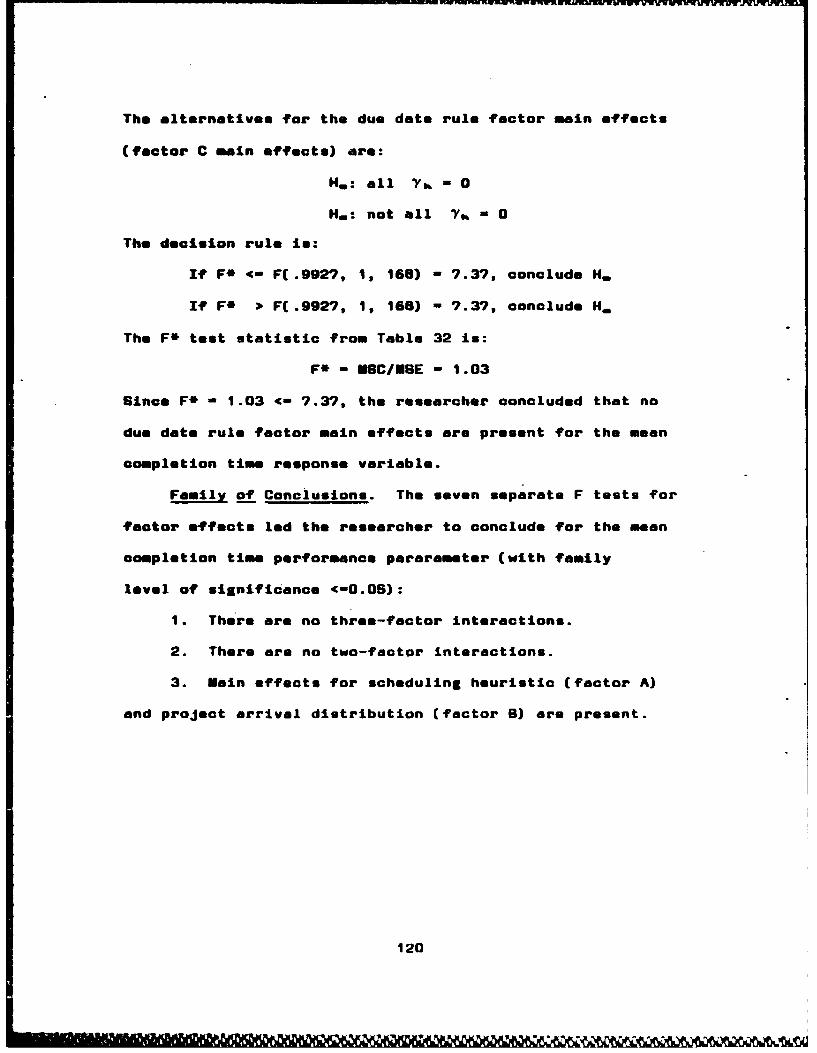
The alternatives for the due date rule factor main effects

(factor C main effects) are:

H.: all 1k - 0

H.: not all Yt - 0

The decision rule is:

If F* 4- F(.992?, 1, 168) ?.3?, conclude H.

If F* ) F(.9927, 1, 168) - ?.3?, conclude H.

The F* test statistic from Table 32 is:

F* - USC/MSE - 1.03

Since F* - 1.03 <- ?.3?, the researcher concluded that no

due date rule factor main effects are present for the mean

completion time response variable.

Family of Conclusions. The seven separate F tests for

factor effects led the researcher to conclude for the mean

completion time performance pararameter (with family

level of significance <-0.06):

1. There are no throe-factor interactions.

2. There are no two-factor interactions.

3. Main effects for scheduling heuristic (factor A)

and project arrival distribution (factor 8) are present.

120

Mean Delay Time

The GAS program code developed for the mean delay'U

time performance parameter is shown in Figure 40. The

output of this source code is an ANOVA table, main and

interaction effects tests, and multiple comparison tests

(Tukey, Bonferroni, and Scheffe). Table 33 shows the ANOVA

table results for the mean delay time performance

parameter.

The seven statistical tests for factor effects and

interaction effects are shown below. The nomenclature for

these tests follow that used by Neter and Wasserman (14).

The A factor is the scheduling heuristic factor, the B

factor is the arrival distribution factor and the C factor

is the due date rule factor for this experiment.

Test for Three-Factor Interactions. The first test was

conducted for three-factor interaction effects. The

alternatives are:

H.: all (a/) 1S.. = 0

H.: not all (0) = 0

The decision rule is:

If F* <- F(.9927, 6, 168) - 3.06, conclude H.

If F* • F(.9927, 6, 168) - 3.06, conclude H.

The F* test statistic from Table 33 is :

F* - M*ABC/M9E - 0.12

Since F* - 0.12 <- 3.06, the researcher concluded that no

ABC interactions are present for the mean delay time

121

options lineeiz-78 pa.esize-6;/* THI PROGRAM WILL PROVIDE A THREE FACTOR FULL FACTORIALANALYSIS OF VARIANCE USING PROC ANOVA ON THE PERFORMANCEPARAMETER ..... PROJECT MEAN DELAY TIME.

date delayber;do eohed-1 to 4;

do dd-l to 2;

do err1v to 3;do obgerv-1 to 8;

Input y 09;output;end;

end;end;

end;carde;

6.01 .86 -2.44 4.43 1.06 -3.45 -3.65 S.26-9.42 -2.0S -7.32 5.51 4.52 -6.17 3.51 17.423.93 -.73 -2.21 3.13 .?S -2.89 -2.06 3.65.S4 .28 .44 .59 .77 .S5 .66 .43.30 .S4 .73 .54 .59 .30 .80 .76.61 .68 .S9 .44 .60 .72 .6? .631.95 .39 .95 2.4S -.20 -.73 -.56 -1.70-S.4S -.38 -5.42 3.49 3.17 -1.07 2.06 10.361.47 -.73 -.26 1.S9 .07 -.85 -.3S 1.76.94 -.90 -2.10 -.34 -1.32 -1.41 -1.98 -. 13-4.04 -.14 -3.52 .11 1.09 -1.82 .94 5.76.84 -.92 -.66 .S7 -.SO -1.16 -1.30 1.214.04 -2.17 -4.36 2.S0 -.80 -3.69 -4.51 1.79-6.34 -1.79 -8.06 S.57 S.26 -3.58 2.83 14.192.S -1.14 -2.08 2.40 .37 -2.06 -.62 2.831.99 1.40 -.20 1.12 1.33 -. 11 -.40 1.49-1.35 -. 63 -2.42 1.97 1.7S 1.01 1.31 2.081.42 .4S .S1 1.25 I.IS -. 13 .44 1.134.15 .4S -2.47 3.50 -.2S -3.19 -1.08 2.34-8.02 -1.63 -6.73 6.13 3.51 -3.71 4.22 14.322.74 -.62 -1.98 3.23 .84 -2.54 -.62 1.761.01 .38 .31 .?9 .86 -.26 .23 .51-.61 -.67 -1.11 -.03 2.SO .11 1.12 -.64.76 .IS -.07 .82 .62 -.S6 .04 .01prod mins;

title "GROUP MEANS FOR PROJECT MEAN DELAY TIME (DAYS)";

" or y;

by ocned dO arriv;prod means;

title "GRAND MEA4 FOR MEAN DELAY TIME';r y;

prod &ov;title "THREE FACTOR ANALYSIS OF VARIANCE ";

close cheda ad arrv;model y- Icned dd arriv Schedidd 10hed~arriv dd*arriv

vChed-4d-arrtw;

Meant eed dd urniv ahedidd eohed*orniv ddeerrivsched*dd*errtv / iaLha-.0073 bon 9Ohefle tukey:

Figure 40. SAS Program-Mean Delay Time

122

U

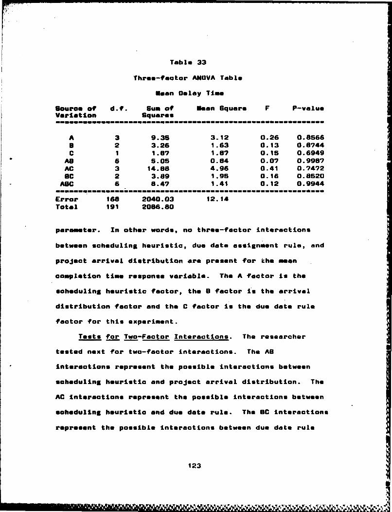
Table 33

Three-factor ANOVA Table

Mean Delay Time

source of d.f. Gum of Mean Square F P-valueVariation Squares

mBmmmmmmmmmmmmmmmmmmmmmmmmnmmBnmmRmmmmminRRmmmminmDmmmmBm m

A 3 9.35 3.12 0.26 0.8566a 2 3.26 1.63 0.13 0.8744C 1 1.87 1.87 0.15 0.6949

AS 6 5.05 0.84 0.0? 0.998?AC 3 14.88 4.96 0.41 0.94?2BC 2 3.89 1.95 0.16 0.8520

ABC 6 8.47 1.41 0.12 0.9944

Error 168 2040.03 12.14Total 191 2086.80

parameter. In other words, no three-factor interactions

between scheduling heuristic, due date assignment rule, and

project arrival distribution are present for the mean

completion time response variable. The A factor is the

scheduling heuristic factor, the 8 factor is the arrival

distribution factor and the C factor is the due date rule

factor for this experiment.

Tests for Two-Factor Interactions. The researcher

tested next for two-factor interactions. The AS

Interactions represent the possible interactions between

scheduling heuristic and project arrival distribution. The

AC Interactions represent the possible interactions between

scheduling heuristic and due date rule. The BC interactions

represent the possible interactions between due date rule

123

". p

and project arrival distribution. The alternatives for the

AS Interactions are:

H.,: all (a$ ).a, - 0

Nm:. not all (ap i. 0

The decision rule Is:

If F* 4- F(.9927, 6, 168) - 3.06, conclude H.

If F* z- F(.9929, 6, 168) - 3.06, conclude H.

The F* test statistic from Table 33 Is:

F- ESAB/ESE - 0.07

Since F* - 0.07 4- 3.06, the researcher concluded that no AS

Interactions are present. No Interactions are present

between the scheduling heuristic and arrival distribution

factors.

The alternatives for the AC Interactions are:

H.: all CaY ) af - 0

H.: not all Cay)17 0

The decision rule is:

If F* 4- F(.9927, 3, 168) - 4.14, conclude H.

If F* 31 F(.9927, 3, 168) - 4.14, conclude H.

The F* test statistic from Table 33 Is:

E*- SAC/ESE - 0.41

Since F* - 0.41 4- 4.14, the researcher concludes that no AC

Interactions are present and therefore no significant

Interactions are present between the scheduling heuristic

and due date rule factors.

124

Thu alternatives for the SC interactions arm:

H.: all Cp -je 0

HM - not all (t3~ )gY 0

The decision rule Is:

If F* ~-F(.992?, 2, 168) - 5.07, conclude H.

If F* F(.9927, 2, 168) - 5.07, conclude H.

The F* test statistic from Table 33 is:

F* - USBC/USE - 0.16

Since F* - 0.16 4- 5.0?, the researcher concluded that no BC

Interactions are present and, therefore, no significant

Interactions are present between the arrival distribution

and due date rule factors.

Tests for Rain Effects. The following tests were

conducted to detect the presence of the min effects of the

experiment. The alternatives for the scheduling heuristic

factor min effects (A main effects) are:

Hw: al I L a - 0

Hm: not all a&. - 0

The decision rule is:

If F* 4- F(.9927, 3, 168) - 4.14, conclude H.

If F* 31 F(.9927, 3, 168) - 4.14, conclude H,.

The F* test statistic from Table 33 Is:

F- USA/USE - 0.26

Since F* - 0.26 4- 4.14, the researcher concludes that A

main effects are not present and, therefore, main effects

for

125

scheduling heuristic are not present for the mean delay

time response variable.

The alternatives far the project arrival distribution factor

maIn effects (B maIn effects) are:

H.: all Pj - 0

Hm: not a11ll 0

The decision rule Is:

If F* 4- F(.9927, 2, 168) - 5.07, conclude H.

If F* 3- F(.9927, 2, 166) - 5.0?, conclude H.

The F* test statistic from Table 33 is:

F- EBB/USE - 0.13

Since F* - 0.13 4- 5.0?, the researcher concluded that

no factor B "ain effects are present and, therefore, arrival

distribution factor "ain effects are not present for the

mean delay time response variable.

The alternatives for the due date rule factor main effects

(factor C main effects) are:

H.: all YK 0

Nm: not all V.K - 0

The decision rule Is:

If F* '-F(.9927, 1, 168) -7.3?, conclude H.

If F* F(.9927, 1, 168) -7.3?, conclude H.

The F* test statistic from Table 33 Is:

F- USC/USE - 0.18

126

Since F* -0.19 <- 7.3?, the researcher concluded that no

due date rule factor main effects are present for the mean

delay time response variable.

Family of Conclusions. The seven separate F tests for

factor effects led the researcher to conclude for the mean

delay time performance parameter (with family level of

significance <- 0.05):

1. There are no three-factor Interactions.

2. There are no two-factor Interactions.

3. Main effects for scheduling heuristic (factor A),

project arrival distribution (factor B), and due date rule

(factor C) are not present.

12?

Standard Deviation of Lateness

The GAG program cods developed for the standard

deviation of lateness performance parameter Is shown In

Figure 41. The output of this source code Is an ANOVA

table, main and Interaction effects tests, and multiple

comparison tests (Tukey, Bonforroni, and Scheffe). Table 34

shows the ANOVA table results for the mean delay time

performance parameter.

The seven statistical tests for factor effects and

Interaction effects are shown below. The nomenclature for

these tests follow that used by Neter and Wasserman (14).

The A factor Is the scheduling heuristic factor, the B

factor Is the arrival distribution factor and the C factor

Is the due date rule factor for this experiment.

Test for Three-Factor Interactions. The first test was

conducted for three-factor Interaction effects. The

alternatives are:

H.: all (aV)i:k = a

H.: not all (aPV)&jft = 0

The decision rule is:

If F* 4- F(.9927, 6, 168) - 3.06, conclude H.

If F* 2 F(.9927, 6, 168) - 3.06, conclude H.

The F* test statistic from Table 34 is :

F* - MBABC/MBE - 0.90

Since F* - 0.90 4- 3.06, the researcher concluded that no

ABC interactions are present for the mean delay time

128

options lineize76 pafesize-66;I* THIS PROGRAM WILL PROVIDE A THREE FACTOR FULL FACTORIALANALYSIS OF VARIANCE uBXMG PROC ANOVA ON THE PERFORMANCEPARANETER..PROJECT STANDARD DEVIATION OF LATENESS TINE.

a/

dote stdloto:do Geoftl- to 4;

do ddint to 2;do arivI to 3;

do obsorv-l to 4;Input y ooutput;and;

end;and;

and;eard@;

36.60 21.00 26.87 31.41 29.38 29.36 25.31 42.4644.09 44.79 41.14 47.69 39.22 37.63 49.06 71.7020.42 24.83 24.43 29.41 21.71 24.4? 24.75 34.422.87 2.44 2.44 2.78 2.47 2.61 2.68 2.683.17 2.50 2.63 3.10 3.41 2.67 3.51 4.152.47 2.67 2.21 2.40 2.47 2.51 2.62 2.7462.62 49.71 41.15 66.24 49.68 42.34 30.01 £0.6?42.24 63.11 11.46 64.13 66.31 47.66 66.g3 94.2649.61 41.61 39.77 47.16 45.02 36.66 35.60 67.6553.66 42.30 38.36 44.11 40.80 31.41 33.03 50.9731.43 51.3? "4.11 46.3? 56.01 41.59 66.93 74.6243.00 38.41 38.26 31.94 30.00 32.14 30.48 49.5029.0? 21.76 21.20 29.20 20.91 22.01 15.78 34.9130.02 35.77 31.22 31.63 29.15 25.61 39.44 61.942f.73 17.76 17.14 22.84 15.77 17.79 16.92 27.8311.49 9.38 9.13 10.44 9.07 9.34 6.01 13.1414.91 13.27 12.76 14.38 12.01 13.29 16.39 19.616.69 7.74 5.10 6.67 7.62 7.61 7.57 9.7024.93 19.97 19.41 21.27 16.11 19.12 16.46 31.0027.92 33.50 30.09 34.63 24.69 24.47 36.89 57.7617.97 11.74 15.12 19.44 15.33 14.63 15.99 24.299.62 9.41 6.39 9.36 6.77 6.79 7.62 10.541&.qS 12.07 12.10 14.36 11.53 12.22 15.73 16.456.26 7.97 7.57 6.41 6.13 7.51 7.43 9.33pro. moons;

title *GROUP MEANS FOR STANDARD DEVIATION OF LATENESS (DAYS)";var Y;,by sch'ed dd arrty;

pro. means;title "GRANO MEAN FOA STANDARD DEVIATION OF LATENESS*;war y;

pie *noveltitle "THREE FACTOR ANALYSIS OF VARIANCE;Glass *Coed dd arriw;model y- sohed del arrty sehed*dd saod*ariv dd*erriv

*cod*dd*@rri v;moons ecaftd dd Orriv tehed*dd safte**orriv dd~orriv

sehod*dd*argiy alae.0073 bon sehaffe tuhey;

Figure 41. SAS Program-Standard

Deviation rif Lateness

129

Table 34

Three-factor ANOVA Table

Standard Deviation of Lateness

source of d.f. Sum of Mean Square F P-valueVariation Squares

A 3 31536.62 10612.94 223.47 0.0000B 2 19205.29 7602.65 323.22 0.0000C 1 4996.70 4996.70 53.11 0.0001

AB 6 16.63 26.44 0.56 0.7601AC 3 3929.35 1309.76 27.84 0.0001BC 2 1037.23 518.62 11.02 0.0001

ABC 6 253.43 42.24 0.90 0.5000

Error 166 7903.31 47.04Total 191 65022.77

parameter. In other words, no three-factor interactions

between scheduling heuristic, due date assignment rule, and

project arrival distribution are present for the standard

deviation of lateness response variable. The A factor is

the scheduling heuristic factor, the B factor is the arrival

distribution factor and the C factor is the due date rule

factor for this experiment.

Tests for Two-Factor Interactions. The researcher

tested next for two-factor interactions. The AB

interactions represent the possible Interactions between

scheduling heuristic and project arrival distribution. The

AC interactions represent the possible interactions between

scheduling heuristic and due date rule. The BC interactLons

represent the possible Interactions between due date rule

130

and project arrival distribution. The alternatives for the

A D I n t e r a t i o n s a r e : . a l ( a 0 ) L - 0

H..- not all (C )., 0

The decision rule Is:

If F* - -FC.9927, 6, 168) - 3.06, conclude H.

If F* F(.9927, 6, 168) - 3.06, conclude H.

The F* test statistic from Table 34 is:

F- USAB/ESE - 0.56

Since F' - 0.56 q- 3.06, the researcher concluded that no AS

Interactions are present. No Interactions are present

between the scheduling heuristic and arrival distribution

factors.

The alternatives for the AC Interactions are:

H.: all (a)as.k - 0

H.: not all (alV),Lq, 0

The decision rule Is:

If F* -c F(..9927, 3, 1683) - 4.14, conclude H.

If F* io F(.9927, 3, 166) - 4.14, conclude H,

The F* test statistic fromn Table 34 is:

F* - ESAC/ESE - 27.84

Sinc F* - 27.84 :o 4.14, the researcher concludes that AC

Interactions are present and therefore significant

Interactions are present between the scheduling heuristic

and due date rule factors.

131

The alternatives for the BC Interactions are:

H.: all (PTY).Ib - 0

H.a: not all (j3V),,ft 0

The decision rule Is:

It F* 4- F(.9927, 2, 168) - 5.07, conclude H.

If F* -v F(.9927, 2, 166) - 5.07, conclude H.

The F* test statistic from Table 34 is:

F- SC/MGE - 11.02

Since F* - 11.02 2- 5.07, the researcher concluded that BC

Interactions are present and, therefore, significant

Interactions are present between the arrival distribution

and due date rule factors.

Tests for lain Effects. The following tests were

conducted to detect the presence of the main effects of the

experiment. The alternatives for the scheduling heuristic

factor maIn effsets (A maIn effects) are:

H.: all a - 0

Hw: not all Of& - 0

The decision rule Is:

If F* <- F(.9927, 3, 166) -4.14, conclude H.

If F* F(.9927, 3, 166) - 4.14, conclude H,.

The F* test statistic from Table 34 Is:

F- USA/USE - 223.4?

Since F* - 223.47 2- 4.14, the researcher concludes that A

main effects are present and, therefore, main effects for

132

scheduling heuristic are present for the standard deviation

of lateness response variable.

The alternatives for the project arrival distribution factor

main effects (B main effects) are:

H.: all PJ " a

H.: not all - 0

The decision rule is:

If F- 4- F(.992?, 2, 168) - 5.0?, conclude H.

If F* 2 F(.9927, 2, 168) - 5.0?, conclude H.

The F* test statistic from Table 34 is:

F* - USE/USE - 53.11

Since F' - 93.11 • 5.07, the researcher concluded that

factor B main effects are present and, therefore, arrival

distribution factor main effects are present for the mean

delay time response variable.

The alternatives for the due date rule factor main effects

(factor C main effects) are:

H.: all Tv - O

H.: not all V, - 0

The decision rule is:

If F' 4- F(.9927, 1, 168) - 7.37, conclude H.

If F' 3 F(.g927, 1, 168) - 7.37, conclude H.

The F' test statistic from Table 34 is:

F' - USC/USE - 323.22

Since F' - 323.22 • 7.37, the researcher concluded that

133

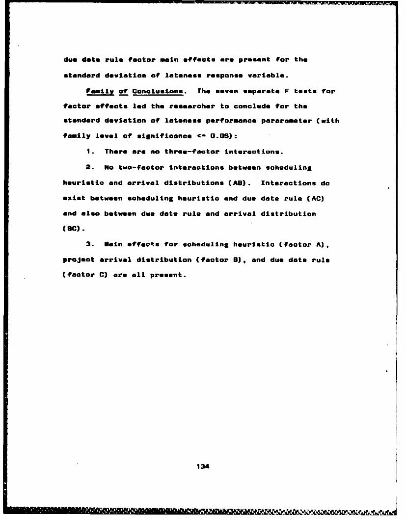
due date rule factor main effects are present for the

standard deviation of lateness response variable.

Family of Conclusions. The seven separate F tests for

factor effects led the researcher to conclude for the

standard deviation of lateness performance pararameter (with

family level of significance 4- 0.05):

1. There are no three-factor interactions.

2. No two-factor interactions between scheduling

heuristic and arrival distributions (AG). Interactions do

exist between scheduling heuristic and due date rule (AC)

and also between due date rule and arrival distribution

(BC).

3. Main effecs for scheduling heuristic (factor A),

project arrival distribution (factor B), and due date rule

(factor C) are all present.

134

Neon Tardiness

The GAS program code developed for the mean tardiness

performance parameter is shown in Figure 42. The output of

this source code is an ANOVA table, main and interaction

effects tests, and multiple comparison tests (Tukey,

Bonferroni, and Scheffe). Table 36 shows the

ANOVA table results for the mean delay time performance

parameter.

The seven statistical tests for factor effects and

interaction effects are shown below. The nomenclature for

these tests follow that used by Meter and Wasserman (14).

The A factor is the scheduling heuristic factor, the B

factor is the arrival distribution factor and the C factor

is the due date rule factor for this experiment.

Test for Three-Factor Interactions. The first test was

conducted for three-factor interaction effects. The

alternatives are:

H.: all (cYI3))LJ, - 0

Hw: not all (apy)akj 0

The decision rule is:

If F* 4- F(.992?, 6, 166) - 3.06, conclude H.

If F* 2 F(.992?, 6, 168) - 3.06, conclude H.

The F* test statistic from Table 35 is :

F* - *GABC/USE - 0.63

Since F* - 0.63 4- 3.06, the researcher concluded that no

ABC interactions are present for the mean tardiness

138

P'i 'q &0~

Options lin~iitiz.76 pagesizo-66:/* THIS PROGRAM WILL PROVIDE A THREE FACTOR FULL FACTORIALANALYSIS OF VARIANCE USING PROC ANOVA ON THE PERFORMANCEPARAMETER..PROJECT MEAN TARDINESS TIME.

data etdleto;do safhed-l to 4;

do ddl1 to 2;

do *rpivli to 3;do obsorv-l to 8;

Input y 02;output;end;

and;and;

end;cards;

16.61 12.27 9.77 15.46 12.24 9.15 6.50 17.611.64 16.22 12.64 21.23 16.12 11.46 20.12 34.1S13.09 9.43 8.36 12.70 10.66 7.67 6.55 14.301.12 .93 1.06 1.22 1.23 1.13 1.22 1.111.10 1.15 1.23 1.26 1.36 1.03 1.92 1.511.13 1.24 1.05 1.06 1.16 1.18 1.22 1.2013.10 11.33 10.09 13.96 11.66 10.65 10.02 13.759.74 15.15 10.16 16.12 16.19 12.39 16.25 25.0311.70 9.70 9.97 12.27 10.57 9.62 9.27 12.6011.61 9.33 6.33 10.66 9.55 9.04 6.10 10.646.29 11.92 6.73 13.10 13.41 10.25 13.15 16.6310.23 6.57 6.69 9.69 6.90 6.56 7.79 10.7213.67 6.22 6.60 12.19 6.37 6.93 5.27 13.676.40 12.91 9.27 17.29 14.66 6.47 16.40 26.659.93 6.95 5.90 10.04 7.96 6.00 7.09 11.735.69 4.20 3.60 4.76 4.56 3.66 3.21 5.555.22 5.36 4.11 6.67 1.97 5.96 6.66 6.124.42 3.63 3.66 4.30 3.61 3.15 3.36 4.4011.60 6.59 6.31 11.06 7.16 5.77 5.96 12.477.50 11.66 6.96 16.06 12.05 7.64 15.66 27.306.22 6.35 5.02 9.04 6.69 4.42 S.77 9.604.54 4.20 3.71 4.35 4.16 3.40 3.36 4.465.21 4.59 4.59 5.92 6.20 4.96 6.51 8.073.91 3.36 3.15 4.04 3.75 2.84 3.22 3.86proc means;

title *GROUP MEANS FOR MEAN TAAOINESS (DAYS)";war y;by lofted dd arriv;

proc aniii;title "GRAND MEAN FOA MEAN TAROINESS';war Y.

proc snows;title "THREE FACTOR ANALYSIS OF VARIANCE "

cloe fened ad arriv;model y- sced dd arriv oched*dd tahed*etriw dd'arriv

softed-dd-rtv;mneans lofted ad arriw scfted*dd sched~orriw ddClrriv

lehotd*dd*arriv /akmho-.018 bon soheffe tukey;

Figure 42. SAG PraogrOM-U n Tardiness

136

Jill ~ ~

Table 35

Three-factor ANOVA Table

Mean Tardiness

source of d.f. Sum of Mean Square F P-valueVariation Square*

mm.mmmmmmmmmmmnmmm..........mininmmnm

A 3 616.82 208.61 20.97 0.0001

87 S6.66 268.33 29.41 0.0001C1 2073.43 1036.72 211.46 0.0001

AS 6 1.82 0.30 0.03 0.9999AC 3 688.22 228.41 23.29 0.00018C 2 173.86 86.78 8.85 0.0002

ABC 6 37.16 6.19 0.63 0.7047

Error 168 1647.28 9.81Total 191 811.94

paramter. In other words, no three-factor Interactions

between scheduling heuristic, due date assigniment rule, and

project arrival distribution are present for the standard

deviation of lateness response variable. The A factor Is

the scheduling heuristic factor, the 8 factor Is the arrival

distribution factor and the C factor Is the due date rule

factor for this experiment.

Tests for Two-Factor Interactions. The researcher

tested next for two-factor Interactions. The AS

Interactions represent the possible Interactions between

scheduling heuristic and project arrival distribution. The

AC Interactions represent the possible Interactions between

scheduling heuristic and due date rule. The BC Interactions

represent the possible interactions between due date rule

137

and project arrival distribution. The alternatives far the

AS Interactions are:

H.,: all Cap ),L - 0

H.: not all (@flaj - 0

The decision rule Is:

If F* 4- F(.9927, 6, 168) - 3.06, conclude H.

If F* F(.992?, 6, 166) - 3.06, conclude H,.

The F* test statistic fromt Table 36 Is:

F* - NSAO/USE - 0.03

Since F* - 0.03 4- 3.06, the researcher concluded that no AS

Interactions are present. No Interactions are present

between the scheduling heuristic and arrival distribution

factors.

The alternatives for the AC Interactions are:

H.W: all Ca'Y)&.t - 0

H.: not all (aY)&f = 0

The decision rule Is:

if F* 4- F(.9927, 3, 166) - 4.14, conclude H.

If F* a, F(.9927, 3, 168) - 4.14, conclude H.

The F* test statistic fromt Table 38 Is:

F* w USACIUSE - 23.29

Since F' - 23.29 :o 4.14, the researcher concludes that AC

Interactions are present end therefore significant

Interactions are present between the scheduling heuristic

and due date rule factors.

138

The alternatives for the OC Interactions are:

Hw: all (PV). - 0

Hw: not all C'y )u., 0

The decision rule Is:

If F* -c- F( .9927, 2, 168) - S.07, conclude H.,

If F* 3, F(.992?, 2, 166) - 5.0?, conclude H,,

The F* test statistic fram Table 35 is:

F* ESBC/UGE - 6.85

Sinc F* - 6.6 .07., the researcher concluded that SC

Interactions are present and, therefore, significant

Interactions are present between the arrival distribution

and due date rule factors.

Tests for Main Effects. The follawing tests were

conducted to detect the presence of the main effects of the

experiment. The alternatives for the scheduling heuristic

factor maIn effects (A m"in effects) are:

Hw: all a a - 0

Hin: not all ci - 0

The decision rule Is:

If F* 4- F(.9927, 3, 166) - 4.14, conclude H.

If F* 2, F(.992?, 3,.168) - 4.14, conclude H.

The F* test statistic from Table 36 Is:

F- MBA/USE - 20.97

Since F* - 20.97 3, 4.14, the researcher concludes that A

"ain effects are present and, therefore, main effects for

139

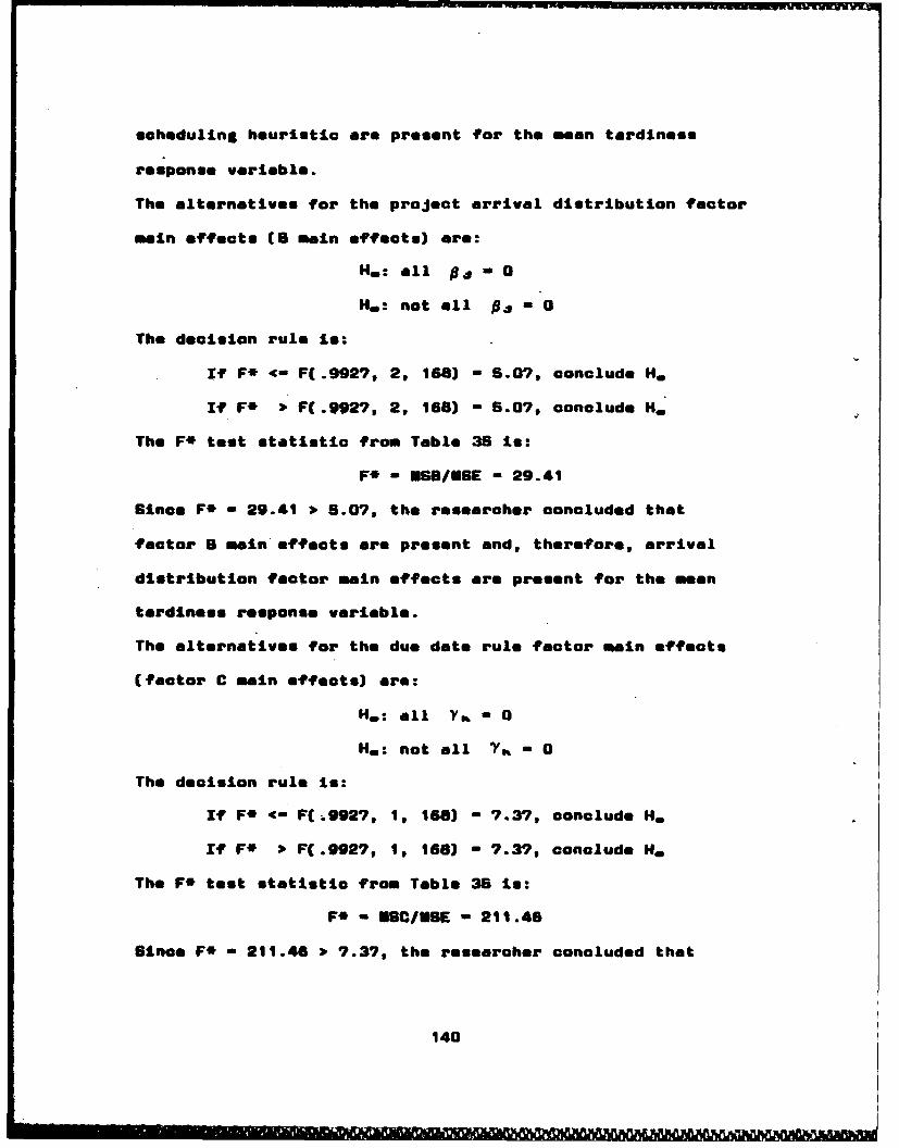
scheduling heuristic are present for the mean tardiness

response variable.

The alternatives for the project arrival distribution factor

"ain effects (B main effects) are:

NW: all ~.-0

H:not all Pa - 0

The decision rule is:

If F* 4mFL.9927, 2, 168) - 5.0?, conclude H.

If F* F(.9927, 2, 166) - 5.0?, conclude H,.

The F* test statistic from Table 36 Is:

F- KGB/USE - 29.41

Since F* - 29.41 2, 6.0?, the researcher concluded that

factor B main effects are present and, therefore, arrival

distribution factor maIn effects are present for the mean

tardiness response variable.

The alternatives for the due date rule factor main effects

(factor C "ain effects) are:

Hw: all VS. - 0

H: not all Ykq - 0

The decision rule Is:

If F* '-F(.9927, 1, 166) - 7.37, conclude H.

If F* F(.992'?, 1, 166) - 7.3?, conclude H.

The F* test statistic from Table 35 Is:

F* -USC/USE - 211.48

Since F* - 211.40 o 7.3?, the researcher concluded that

140

due date rule factor min effects are present for the

standard deviation of lateness response variable.

Family of Conclusions. The *sven separate F tests for

factor effects led the researcher to conclude for the

standard deviation of lateness performano parerameter (with

family level of significance 4- 0.06):

1. There are no three-factor interactions.

2. No two-factor Interactions between scheduling

heuristic and arrival distributions (AS). Interactions do

exist between scheduling heuristic and due date rule (AC)

and also between due date rule and arrival distribution

(Boc).

3. Main effects for scheduling heuristic (factor A),

project arrival distribution (factor B), and due date rule

(factor C) are all present.

141

BibI lofraphy

I. Baker, Kenneth R. wsequenoing Rules and Due-DateAssignments In a Job Shop,O Eansement Science, 30:1093-1104 (September 1964).

2. Bookbinder, Jams H. and Afzal Ibn Moor. "SettingJob-Shop Due-Dates with Service-Level Constraints,'Journal of the 0 erational Research Society 36:10,17-1026 (November 1968).

3. Chang, T.C.E. 00ptimal Due-Oats Assignment in a JobShop," International Journal of Production Research.24: 803-818 (May-June 1966).

4. Conway, Riohard 0. Theory of Scheduling. Reading:Addison-Wesley Publishing Company, 1967.

S. Dumond, John. Evaluation of Due Date Assignment Rulesfor Dynamically Arriving Projects. PhD Dissertation.Indiana University, B1loom ington IN, 198.

6. Dumond, John. Evaluating Project Scheduling and DueDate Asslgmnt Procedures!:.An Experiment Analysis.Working Paper Series WPS 66-30. College ofAdministrative Science, Ohio State University ON,February 1996.

7. Elsayed, E.A. and N.Z. Nar. "Heuristics for ResourceConstrained Scheduling,a International Journal ofProductionResearch. 24: 299-310 (March-April 1986).

6. Cray, Capt Cary. rho plcat ion of the ComputrSppored Network Analyst* a!MiatemsoCSN) to0Acquisit ion Management aAplied tothe reisionStrike Systeom (PS) M Thesis, AFIT/SLN/LSY/66-29. School of Systems and Logistics, Air For'ceInstitute of Technology (AU), Wright Patterson AFBOH, September 1966.

9. Hall, Nicholas 9. 0Scheduling Problems with General-ized Due Dates," IE Transactions, 16: 220-222(June 1966).

10. Harrison, F.L. Advanced Project Management. Now York:Halsted Press, 1961.

11. Kerznor, Harold. *Co mme rally Available ProjectTracking Systems," Project Management Journal, 1789-97 (September 1966).

142

12. Lock, Dennis. Project Management Handbook. England:IGower Technical Press Limited, 1967.

13. Moder, Joseph J. and others. Project Management with

CPPERT, and Precedence Diear amn n. New York:Van Nostrand Reinhold Company, 1963.

14. Meter, John and 8illiam Wasserman. Applied LinearModels (Second Edition). Homewood IL: Richard D.Irwin, Inc., 1986.

1S. Patterson, James H. "Exact end Heuristic SolutionProcedures for the constrained Resource ProjectScheduling Problem, a monograph, Vol*. I-IV.November 1962.

16. Petterson, James H. "A Comparison of Exact ApproachesFor Solving The Multiple Constrained Resource, ProjectScheduling Problem, Mangement Science, 30: 84-86?(July 1964).

17. Pritsker, Alan B. Introduction to SLAM and SLAM X1.Now York: Helsted Press, 1986.

1S. Russell, Robert A. *A Comparison of Heuristics forScheduling Projects with Cash Flows and Resource

(October 1966).

19. BAS Introductory guide (Third Edition). Cary, NC:

BAB Institute Inc., 1968.

143

VITA

Captain James D. Martin was barn on 19 October 1958 In

Minneapolis, Minnesota. He graduated from high school In

Waukesha, Wisconsin, in 1976 and attended the University of

Wisonsin, from which he received the degree of Bachelor of

Science in Mechanical Engineering in May 1982. Upon

graduation, he received a commission in the USAF through the

ROTC program. He was called to active duty and assigned to

the Headquarters Ballistic Missile Office at Norton AFB,

California In July 1982. He served as a project manager for

Defense Suppression Systems, Advanced Strategic Missile

Systems until entering the School of Systems and Logistics

Management, Air Force Institute of Technology, in June 1986.

Permanent address: 8719 Chuker Drive

Dayton, Ohio 45424

144

iREPORT DOCUMENTATION PAGE 0010 Oft 070"-IN"Ia. V= 11lb. RESTRICTIVE MARKINGS

Z&SCF ASFCTION AUTHORITY 3. DISTRIBU IN /AVAILABILITY OF REPORT

~. ~ Aprroved for public release;

INRORMING ORGANIZATION REPORT NUMBER(S) S. MONITORING ORGANIZATION REPORT NUMIER(S)

APTIGSIILsyI87-19________________________Es. AME P PMON G ORGANIZATION 6Gb. OFFICE SYMBOL 7a. NAME OF MONITORING ORGANIZATION

School of System (if &PWaid Lo~istics ________________________

GL ADDRESS (Cuy, Stat an PC*' 7b. ADDRESS (Guy, SUaM. and ZIPCode)Air Force Institute of Technology (AU)

- Wtight-Patterson An, Chiio 45433-6583

EsL NAME OP FUNDING/ SPONSORING B b. OFFICE SYMBOL. 9. PROCUREMENT INSTRUMENT IDENTIFICATION NUMBERORGANIZATION j p~ak

Ift AOMRESS Oey. Stawand ZFCods) 10. SOURCE OF FUNDING NUMSERS-

PEOGM No PROJECT ITASK MWORK UNITEENTN. NO. 1 No 0O NO.

11. TITLE ("*a* hawil Ossftaefon)AN EVALUA!I; OF PROJET SMWEULD TECHNQUE IN A DWIC ENIRONMENT

1I. PEKNLAUHRS

James D. Martin. Ct.USAF134. TYPEl OF REPORT I 3b. TIME COVERED To114. DAEOF REPORT (Year, MAkOft) IS. PAGE COUNT

MS Thesis F ROM TOI 1987 Sentamnhr I 1g16. SUPPLEMENTARY NOTATION

17. COSATI CODES 15. SUBJECT TERMS (Conthbs on rovem if necesmy &Wd WenUIf by block number)FIELD GROUP SUB-GROUP PER-T/CPH, Project Scheduling, Due Date Assigrunent Rules,050 Scheduling Heuristics, Project Arrival Distributions

19. ABSTRACT M(Condbiu on mevere if necoaty lend Jdentfl4 by block number)

Thesis Chairman: John Duond, Lt Col, UISAFAsst Prof of Systems mangsneent

F III=. nl~am~ LAW An s.qpF

wdgha.Fwleua Ara oil 4"Na

20. DISTRIBUTION/ AVAiLABIUTY OP ABSTRACT 21. ABSTRACT SECURITY CLASSIFICATIONOUNCASSIIEDIUNUIMITED 03 SAME AS RPT. C) OTIC USERS U0tLASSIFIED

220. NAME OF RESPONSIBLE INDIVIDUAL 22b. TELEPMONE (include Ame Code) 22c. OFFICE SYMBOLJohn Diamod. Lt Col. USAF AFIT/LSY

00F~em 473. JUN If Previous ed~tons are obsolete. SECURITY CLASSIICATION OF THIS PAGE

UCLASSIFIED

UNCLASSIFIED

Block 19. Abstract

9This research found, in general, that different projectarrival distributions do affect the performance ofscheduling heuristics and due date setting rules in anabsolute sense, but not In a relative sense. Mecause ofthts, the project manager does not really need to beconcerned about the-arrival distribution of now projects.

The best results are obtained when the Scheduled Finish

Tim CFT) due date setting rule is applied. Not allproject managers could implamentthIs'procedure due to thecomputer hardware/software requirements, financialconstraints, project duration uncertainty, resourceconstraints, etc.. If they could use the OFT rule to setthe due date of the arriving project, they would be wise touse the very simple First-!n-First-Served (FIFU) schedulingheuristic to allocate resources to the project.

An alternative to project managers would be to choosethe easier to implement CPTIME due date rule. If this isthe case then the manager would want to choose either the8AUtDDI or the UINLFT[DO] rule which produce similarresults using the CPTZtE due date rule.

This research has determined that the relativeperformance of the tested scheduling heuristics and due datesetting rules is unaffected by the project arrivaldistribution. For the project manager, this confirms thatcertain scheduling heuristics, due date assignment rules,and combinations thereof will perform better than othersregardless of th, project arrival distribution. Therefore,the alternatives iq management are 1) accept the decrease inperformance capability for the easier to implement CPTIMEdue date assignment rule used with the due date orientedheuristics; or 2) make the necessary commitments andInvestments to. ipleme t at least one of these heuristicscombined with the OFT dae date assignment procedure orbetter yet; 3) implement the FIFO/SFT combination forassured performance.

UNCLASSIFIED

AI/pzmft

1qgg