Theoretical Computer Science 374 (2007) 170–180www.elsevier.com/locate/tcs

An external-memory depth-first search algorithm for general gridgraphsI

Jun-Ho Her, R.S. Ramakrishna∗

Department of Information and Communications, Gwangju Institute of Science and Technology, 1 Oryong-dong, Buk-gu, Gwangju 500-712,Republic of Korea

Received 18 November 2005; received in revised form 14 December 2006; accepted 22 December 2006

Communicated by J. Diaz

Abstract

Graph data in modern scientific and engineering applications are often too large to fit in the computer’s main memory.Input/output (I/O) complexity is a major research issue in this context. Minimization of the number of I/O operations (in externalmemory graph algorithms) is the main focus of current research while classical (internal memory) graph algorithms were designedto minimize temporal complexity.

In this paper, we propose an external memory depth first search algorithm for general grid graphs. The I/O-complexity ofthe algorithm is O(sort(N ) log2

NM ), where N = |V | + |E |, sort(N ) = Θ( N

B logM/BNB ) is the sorting I/O-complexity, M is

the memory size, and B is the block size. The best known algorithm for this class of graph is the standard (internal memory)DFS algorithm with appropriate block (sub-grid) I/O-access. Its I/O-complexity is O(N/

√B). Recently, the authors proposed an

O(sort(N )) algorithm for solid grid graphs.c© 2007 Elsevier B.V. All rights reserved.

Keywords: I/O-complexity; External-memory algorithms; Graph algorithms

1. Introduction

In the modern computer industry, performance of storage systems is found to be unacceptably poor in comparisonwith that of the computing system as a whole. The block access latency and bandwidth of traditional magnetic disksare far behind computing speeds. The disk is unlikely to catch up: the gap will only widen [18]. Although highperformance storage systems such as redundant arrays of inexpensive disks (RAID) [19,20,25] rekindle some hope,the gulf between computing systems and storage systems is still very wide and input/output (I/O) costs threaten to bea major performance bottleneck in computations involving massive data sets.

External memory algorithms have attracted considerable attention of late. The focus of these research efforts isto effectively deal with voluminous data that characterize many applications [23]. These algorithms – also called

I This work is supported by BK21 and Foreign Professor Support Project of GIST.∗ Corresponding author. Tel.: +82 62 970 2217; fax: +82 62 970 2204.

E-mail addresses: jhher@gist.ac.kr (J.-H. Her), rsr@gist.ac.kr (R.S. Ramakrishna).

0304-3975/$ - see front matter c© 2007 Elsevier B.V. All rights reserved.doi:10.1016/j.tcs.2006.12.022

CORE Metadata, citation and similar papers at core.ac.uk

Provided by Elsevier - Publisher Connector

J.-H. Her, R.S. Ramakrishna / Theoretical Computer Science 374 (2007) 170–180 171

Fig. 1. The relationships among several sparse graph classes.

out-of-core algorithms – offer an algorithmic approach to counter the (in)famous I/O bottleneck between the twolevels (internal and external) of memory. Many researchers have tried to exploit locality of reference for improvingI/O-efficiency of out-of-core algorithms.

External memory graph algorithms are the need of the day because large scientific and engineering applicationsfrequently challenge the computer’s ability to confront massive graph data. Although a large number of I/O-efficientgraph algorithms are known [2–5,7,13,14,17], a number of important problems still remain open.

In this paper, we consider the depth first search (DFS) problem for a specific graph class, namely grid graphs. Agrid graph is a finite node-induced subgraph of the infinite two-dimensional integer grid. It may be non-planar owingto intersecting diagonal edges. DFS is used in many application areas such as artificial intelligence [6] as well as inmany higher-level graph algorithms. However, no optimal external memory DFS algorithm is known for arbitrarysparse graphs. For two classes of graph – planar graphs and grid graphs –, improved external memory DFS algorithmshave been proposed in [2] and [14], respectively. However, the latter has room for further improvement because itdoes not fully exploit the structural characteristics of grid graphs. Recently, the authors proposed an external memoryDFS algorithm for a specific grid graph, viz., the solid grid graph [9]. Appendix details definition of grid graphs andsolid grid graphs. In Fig. 1, an oval has been added for solid grid graphs on the Venn diagram presented in [15].

This paper proposes an I/O-efficient DFS-algorithm for general grid graphs.

1.1. Model of computation (Two-level I/O model)

We design and analyze the algorithm under the standard two-level I/O model proposed in [1].The model works with four parameters:

N is the problem size in units of data items (in graph problems, N = |V | + |E |),M is the internal memory size in units of data items,B is the disk block transfer size in units of data items, andD is the number of independent disk drives (i.e., number of blocks that can be transferred concurrently),

where M < N and 1 ≤ DB ≤ M/2. Initially, all the data is stored on disk and an I/O-operation transfers D blocksof consecutive elements between disk (external memory) and internal memory. The complexity of an algorithm inthis model is the number of I/O-operations it performs. The I/O-complexities of scanning and sorting (N contiguousitems) are known to be scan(N ) = Θ( N

DB ) and sort(N ) = Θ( NDB logM/B

NB ), respectively [1].

In this paper, we restrict our discussion to the single-disk (D = 1) case.

1.2. Previous results

The best known DFS-algorithms for general undirected graphs incur O(|V | +|V |

M ·scan(|E |)) [7] orO((|V |+scan(|E |)) · log2 |V |) [12] I/Os. The latter algorithm outperforms the former on most graphs except verysparse graphs (i.e. G(V, E) s.t. |E | ≤ |V |). For general directed graphs, the best known external memory DFS-algorithm has an I/O-complexity of O((|V |+scan(|E |)) · log2

|V |

B )) [5]. An improved algorithm has been devised fora special class of graphs, namely, planar graphs [2]. This algorithm is a combination of an O(sort(N )) I/O reduction

172 J.-H. Her, R.S. Ramakrishna / Theoretical Computer Science 374 (2007) 170–180

from DFS to BFS (Breadth First Search) [2] and an O(sort(N )) I/O BFS algorithm for embedded planar graphs [13].As a consequence, its I/O-complexity is O(sort(N )). For (possibly non-planar) grid graphs, a O(N/

√B) algorithm

has been proposed in [14]. This algorithm is similar to the standard internal memory DFS-algorithm with additional,carefully crafted block (sub-grid) I/O access. For solid grid graphs, an O(sort(N )) algorithm has been proposed bythe authors [9]. This algorithm transforms a given solid grid graph to an embedded planar graph I/O-efficiently andcomputes a DFS-tree of the original graph from the DFS-tree of the transformed graph I/O efficiently.

The I/O-complexity of the algorithm that we propose is O(sort(N ) log2NM ). The well known divide-and-conquer

approach for planar graphs is judiciously crafted to deal with (nonplanar) grid graphs. Further, we assume that theinput planar graph and the input grid graph are biconnected. Even if the connected input graph is not biconnected, onecan compute biconnected components of the graph in O(sort(N )) I/Os [15]. In the DFS-tree problem, the divide-and-conquer strategy is deployed on the biconnected components of the graph. Section 3.1 of [2] provides the details ofthis strategy. We also assume that each vertex of the input grid graph has integer coordinates.

The rest of this paper is organized as follows: Section 2 contains a review of a planar DFS algorithm relevant toour work. In Section 3 we describe the proposed algorithm. Finally, Section 4 provides concluding remarks and someopen problems. We collect some graph theoretic fundamentals in the Appendix.

2. A DFS algorithm for planar graphs

The DFS algorithm for planar graphs in [2] (Planar DFS) is based on the divide-and-conquer approach proposedin [21]. We briefly review Planar DFS because our algorithm is based on this algorithm. Planar DFS is outlinedbelow.

1. Compute a simple cycle 23 -separator C of G. (I/O-complexity: O(sort(N)).)

2. Find a path P from s to some vertex v in C . (I/O-complexity: O(sort(N)) using an I/O-efficient breadth-first searchalgorithm.)

3. Extend P to a path P ′ containing all vertices in P and C . (I/O-complexity: O(scan(N)).)4. Compute the connected components H1, . . . , Hk of G \ P ′.

For each Hi , find the vertex vi ∈ P ′ furthest away from s along P ′ s.t. there is an edge {ui , vi }, ui ∈ Hi . H1, . . . , Hkcan be computed in O(sort(N )) I/Os. Also, v1, . . . , vk can be found in O(sort(N )) I/Os.

5. Recursively compute DFS-trees for components H1, . . . , Hk , rooted at u1, . . . , uk and merge T1, . . . , Tk , path P ′,and edges {ui , vi }.

The overall I/O-complexity is O(sort(N ) log2NM ). The following lemma is used to prove the correctness of our

algorithm.

Lemma 1 ([2]). The tree T computed by the above algorithm is a DFS-tree of G.

Further details can be found in [2] but here we review Step 1 of the above algorithm in detail because this subroutineplays a part in our algorithm. A simple cycle 2

3 -separator C of an embedded planar graph G is a simple cycle whichis such that neither the subgraph inside nor the one outside the cycle contains more than 2

3 |V | vertices. Such a cycleis guaranteed to exist only if G is biconnected. An algorithm to compute a simple cycle 2

3 -separator of an embeddedbiconnected planar graph I/O-efficiently has been studied in [2]. The main idea is similar to the ones found in [11,16].Here is a brief on this algorithm (Planar 2

3SCS):

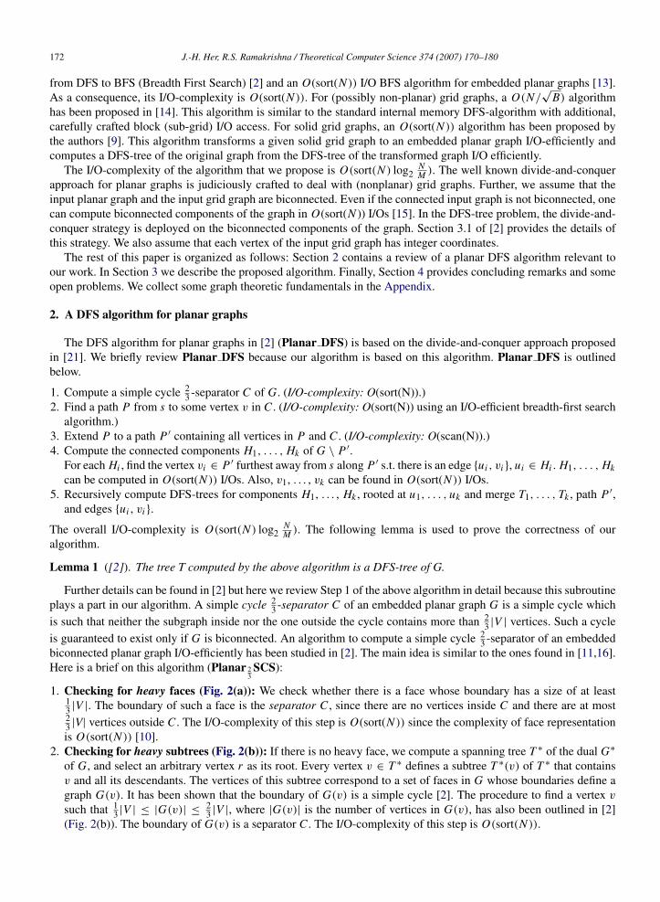
1. Checking for heavy faces (Fig. 2(a)): We check whether there is a face whose boundary has a size of at least13 |V |. The boundary of such a face is the separator C , since there are no vertices inside C and there are at most23 |V| vertices outside C . The I/O-complexity of this step is O(sort(N )) since the complexity of face representationis O(sort(N )) [10].

2. Checking for heavy subtrees (Fig. 2(b)): If there is no heavy face, we compute a spanning tree T ∗ of the dual G∗

of G, and select an arbitrary vertex r as its root. Every vertex v ∈ T ∗ defines a subtree T ∗(v) of T ∗ that containsv and all its descendants. The vertices of this subtree correspond to a set of faces in G whose boundaries define agraph G(v). It has been shown that the boundary of G(v) is a simple cycle [2]. The procedure to find a vertex v

such that 13 |V | ≤ |G(v)| ≤

23 |V |, where |G(v)| is the number of vertices in G(v), has also been outlined in [2]

(Fig. 2(b)). The boundary of G(v) is a separator C . The I/O-complexity of this step is O(sort(N )).

J.-H. Her, R.S. Ramakrishna / Theoretical Computer Science 374 (2007) 170–180 173

Fig. 2. (a) A heavy face. (b) A heavy subtree. (c) Splitting a heavy subtree.

3. Splitting a heavy subtree (Fig. 2(c)): The above two steps may fail to find a simple cycle 23 -separator of G. This

points to a unique situation in which for every leaf l ∈ T ∗ (face in G), we have |G(l)| < 13 |V |; for the root r of

T ∗, we have |G(r)| = |V |; and for every other vertex v ∈ T ∗, either |G(v)| < 13 |V | or |G(v)| > 2

3 |V |. Thus, therehas to be a vertex v with |G(v)| > 2

3 |V | and |G(wi )| < 13 |V |, for all children w1, . . . , wk of v. The computation

of a subgraph G ′ of G(v) consisting of the boundary of the face v∗ and a subset of the graphs G(w1), . . . , G(wk)

such that 13 |V | ≤ |G ′

| ≤23 |V | can be found in [2]. It must be noted that the boundary of G ′ is a simple cycle [2].

This step has an I/O-complexity of O(sort(N )).

The following theorem pertains to the I/O-complexity of Planar 23SCS.

Theorem 2 ([2]). A simple cycle 23 -separator of an embedded biconnected planar graph can be computed in

O(sort(N )) I/O operations. The computation has linear space-complexity.

3. Proposed algorithm

3.1. Some terms

Here are some terms used in the sequel. A simple cycle which is such that the number of vertices in its interior andexterior parts does not exceed 2

3 |V | is a simple cycle 23 part recognizer. A connector is a diagonal edge that connects

the interior and the exterior parts (of a cycle). A path connector is a longest simple path that includes a connector suchthat the degree of each internal vertex is exactly two. A path compensator is a path that includes at least one end-vertexof each connector (or a terminal vertex of each path connector). A cycle 2

3 part recognizer, when augmented with apath compensator, separates the interior part from the exterior part. Fig. 3 shows a section of the cycle part recognizerand (path) connectors in a section of the grid graph.

3.2. Overview

The divide-and-conquer approach of Planar DFS can be applied to the DFS problem for general grid graphs aftersome modifications. In this section, we make two observations related to a simple cycle in general grid graphs.

Observation 1. A simple cycle of a grid graph cannot separate the graph into interior and exterior parts because ofdiagonal edges that cross the cycle.

Observation 2. A simple cycle of a grid graph can separate the graph if it is augmented with an end-vertex of eachconnector (or a terminal vertex of each path connector).

We extend Planar DFS to general grid graphs as follows (refer to Fig. 4):Input: A general grid graph GOutput: A depth-first search tree T of G

174 J.-H. Her, R.S. Ramakrishna / Theoretical Computer Science 374 (2007) 170–180

Fig. 3. The fattest gray line is a portion of a cycle part recognizer. The thick black lines represent (path) connectors; the two consecutive fat linesrepresent two path connectors and the two single heavy lines represent two connectors.

Fig. 4. Outline of the algorithm: The broken line is a simple cycle 23 part recognizer C . The connected components of G \ PI excepting Hx are

shaded black. The connected component Hx includes the areas shaded light gray and dark gray; the biconnected component Hxy is shaded lightgray. The other biconnected components of Hx are shaded dark gray. Heavy lines represent the path compensator PI I that includes connectors ofHxy .

1. Compute a simple cycle 23 part recognizer C of G. (I/O-complexity: O(sort(N )). Please see Section 3.3.)

2. Find a path P from s to some vertex v in C .This step is the same as Step 2 of Planar DFS.

3. Extend P to a path PI containing all the vertices in P and C .This step is the same as Step 3 of Planar DFS.

4. Compute the connected components H1, . . . , Hk of G \ PI . For each Hi , find the vertices vi ∈ PI furthest awayfrom s along PI such that there is an edge {ui , vi }, ui ∈ Hi . This step is the same as Step 4 of Planar DFS.

5. If a connected component Hx whose vertex cardinality is greater than 23 |V | exists, then

A. Find biconnected components Hx1, . . . , Hxl . (I/O-complexity: O(sort(|V |)) [15].)B. If a biconnected component Hxy whose vertex cardinality is greater than 2

3 |V | exists, thena. Compute a path compensator PI I . (I/O complexity: O(sort(N )). Please see Section 3.4)b. Compute the connected components Hxy1, . . . , Hxym of Hxy \ PI I . For each component Hxy j , find the vertex

vxy j ∈ Hxy j furthest from sxy (or ux ) along PI I such that there is an edge {uxy j , vxy j }, uxy j ∈ Hxy j . We canalso adopt Step 4 of Planar DFS for this step. Its I/O-complexity is O(sort(N )).

6. Recursively, compute DFS-trees of H1, . . . , Hx1, . . . , Hxy1, . . . , Hxym, . . . , Hxl , . . . , Hk , and construct a tree Tby merging them, the paths PI , PI I , and edges {ui , vi }, {uxy j , vxy j }.

Lemma 3. The tree T computed by the above algorithm is a DFS-tree of G.

Proof. In view of Lemma 1, we need only to show that Tx is a DFS-tree of the component Hx . For each biconnectedcomponent Hx1, . . . , Hxy, . . . , Hxl , we can complete a DFS-tree Tx of Hx by merging their DFS-trees by a procedurethat is similar to the one in [2]. We have to show that Txy is a DFS-tree of the biconnected component Hxy .

It is seen that Txy consists of DFS-trees of Hxy1, . . . , Hxym , a path PI I , and edges {uxy j , vxy j }. Thus, Txy spansHxy . By Lemma 6, the path PI I is simple. All non-tree edges with both end-vertices in a component Hxy j are back-edges (this is trivial because we compute DFS-trees for Hxy j ). For every non-tree edge {v, w} with v ∈ PI I andw ∈ Hxy j , w is a descendant of the root uxy j of the DFS-tree Txy j . The tree Txy j is connected to PI I through the edge

J.-H. Her, R.S. Ramakrishna / Theoretical Computer Science 374 (2007) 170–180 175

{vxy j , uxy j }. By the choice of vertex vxy j , v is an ancestor of vxy j , and thus an ancestor of uxy j and w. Therefore, theedge {v, w} is a back-edge. �

Each recursive call in Step 6 processes a subgraph (of G) consisting of at most two-thirds of the vertices of thegraph from the previous recursive call. The recursion is continued until the size of the current graph is less than orequal to the size of the main memory (M). Thus, the number of calls is bounded by O(log2

NM ). As already pointed

out, the total I/O complexity of the other computations is O(sort(N )). Consequently, we arrive at Theorem 4, the mainresult of this paper.

Theorem 4. A DFS-tree of a general grid graph can be computed with O(sort(N ) log2NM ) I/O operations.

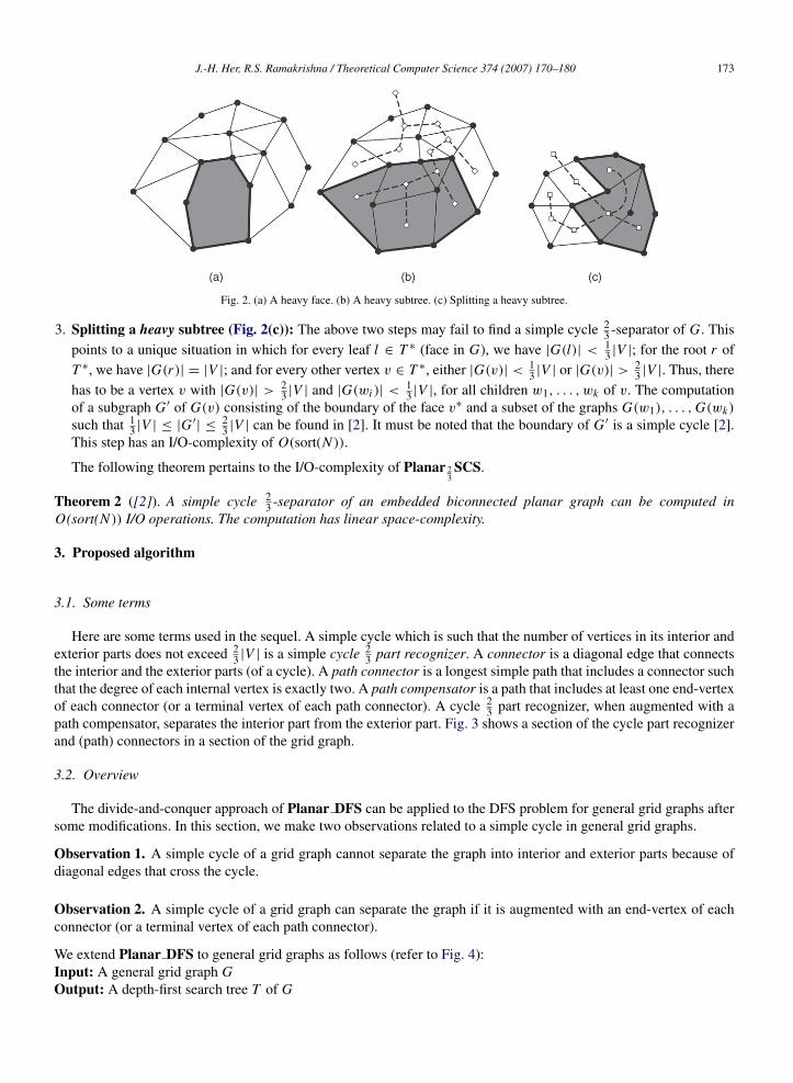
3.3. Finding a simple cycle 23 part recognizer C

In this section, we describe a procedure to compute a simple cycle 23 part recognizer C of a grid graph G. The

idea is to find an embedded planar subgraph of the given grid graph whose vertex cardinality (counting isolated innervertices) is at least 2

3 |V | and then to allow Planar 23SCS to work on this subgraph. We can find an embedded planar

subgraph of a biconnected grid graph by considering the graph as the union of at most two (layered) embeddedplanar subgraphs with extra edges connecting them as depicted in Fig. 5(a). We can recognize this decompositionby identifying (overlapped) faces of the grid graph with the help of certain computations in the face identificationalgorithm [10].

We compute the cycle C of G as follows:

1. Identifying (overlapped) facial cycles:A. Remove an edge of each intersecting diagonal edge pair if at least two vertical (horizontal) edges exist in the

considered cell (the cell is defined in Appendix). Let the resulting graph be G(= (V, E)).B. Compute the directed graph G = (V , E) for G (see Fig. 5(c)).

a. For each edge {u, v} ∈ E , add two vertices v(u,v) and v(v,u) to V .b. For each vertex u ∈ V , sort its incident edges in counterclockwise order (let these sorted edges be

{u, v0}, . . . , {u, vl−1}).c. Add directed edges (v(vi ,u), v(u,v(i+1) mod l )) to E , where 0 ≤ i < l.

C. Compute the connected components of G (by considering the edges of G as being undirected).D. Compute the cycles of G which correspond to these connected components.E. For each cycle, if it is simple, then add it to C .F. Break each non-simple cycle into several simple cycles. A simple cycle results on encountering a repeated

vertex while traversing the cycle along the corresponding directed edges of G. Add the resulting simple cyclesto C .

2. Extracting an embedded planar subgraph G ′:A. Copy G to G and copy C to C .B. Select a cycle in C and remove all the edges intersecting with those of the cycle in G.C. Select a cycle that shares at least one edge with the current cycle without actually crossing it (such a cycle will

be called a cocycle in this paper). Remove the current cycle from C . Remove all the edges intersecting withthose of the cycle in G. Iterate the process until no cycle remains in C .

D. Select a cycle in C which is intersecting with the cycle of Step 2B. Remove all the edges intersecting with thoseof the cycle from G.

E. Select a cocycle of the current cycle and remove the current cycle from C . Remove all the edges intersectingwith those of the cycle in G. Iterate the process until no cycle remains in C .

F. Delete each pendant vertex along with the incident edge. Recursively do this for its adjacent vertex (this is toremove the simple subpaths in G and G so that they become biconnected). See Fig. 5(g) and (h).

G. Calculate the number of isolated vertices in the exterior of G and G. Let the graph with a smaller number ofisolated vertices in its exterior be G ′.

176 J.-H. Her, R.S. Ramakrishna / Theoretical Computer Science 374 (2007) 170–180

Fig. 5. Finding a simple cycle 23 part recognizer C : (a) Double layered planar structure of a general grid graph (one consists of heavy black lines

and the other consists of heavy gray lines). (b) The input (general) grid graph G (the broken lines are to be removed in Step 1A). (c) The directedgraph G on G. (d) Broken lines form the cycle corresponding to the connected components built with broken arrows (dark broken lines constitutethe union of the simple cycles after Step 1F). (e)–(f) Two layers of the cycles in (d) (dark broken lines). (g)–(h) G and G. Gray vertices and graylines are removed after Step 2F. In this case, any one of them could be reported as G′ since the number of isolated exterior vertices are the same.(i) Dark heavy lines represent the final 2

3 part recognizer C after executing Planar 23

SCS.

3. Adopting Planar 23SCS: We deploy Planar 2

3SCS on the subgraph G ′. Here, it is possible that an isolated vertex

(or a connected component) has resulted as a consequence of the removal of an edge in the interior of a face. Inthis case, the isolated vertex of a face f still contributes to the vertex cardinality of f and we include the exteriorvertices of G ′ in computing the total vertex cardinality |V | while detailing Planar 2

3SCS. An example of this step

is shown in Fig. 5(i).

Lemma 5. A simple cycle 23 part recognizer of a biconnected grid graph can be computed with O(sort(N )) I/O

operations.

J.-H. Her, R.S. Ramakrishna / Theoretical Computer Science 374 (2007) 170–180 177

Proof. Correctness: We show that the number of isolated vertices in the exterior of G ′ (|Viso|) is less than 13 |V | with

a view to guaranteeing that a simple cycle 23 part recognizer exists in G. Since the algorithm selects the graph which

has a smaller number of isolated vertices in its exterior, the worst case occurs when two planar layers have almost thesame number of isolated vertices in the exterior as in Fig. 5(a). Here, G ′ could be obtained from any one of the twolayers. Denote the vertices on the boundary of the outer face of G ′ by Vout . As can be seen in the figure, each isolatedexterior vertex appears after every two vertices of Vout (except at each corner). Thus, for sufficiently large grid graphs,|Viso|/|Vout | ≈ 1/2. Without loss of generality, |V − Viso − Vout | = α|V | for a non trivial grid graph (0 < α < 1).Then, |Viso| ≈

1−α3 |V |. Thus, |Viso| < 1

3 |V |.Since we remove all the edge-crossings in Step 2, the resulting subgraph G ′ is (embedded) planar. Thus, we can

employ Planar 23SCS in Step 3 on the subgraph. As isolated vertices within a face contribute to the vertex cardinality

of the face, and all the vertices of Viso are included in computing the total vertex cardinality |V | of Planar 23SCS, the

simple cycle 23 separator of the planar subgraph after Step 3 plays the role of a simple cycle 2

3 part recognizer in thegiven biconnected grid graph.

Complexity: In Step 1A, we consider a reference vertex in a grid cell say, the upper left vertex. For the referencevertex (i, j), if there are edges (i + 1, j), (i, j + 1) and (i, j), (i + 1, j + 1), then this cell contains an intersectingdiagonal edge pair. Thus Step 1A performs O(scan(N )) I/Os. Step 1B requires O(sort(N ))I/Os since this step is theface identification algorithm [10]. Step 1C takes O(sort(N ))I/Os [7]. Steps 1D and 1E consume O(scan(N )) I/Os eachsince there should be a constant number of cycles with size O(N ). The simple cycle extraction in Step 1F is executed(Fig. 5(d)) as follows.

We order the vertices of Cns (cycle in the figure) along the directed edges of G as [1, 2, 3, 4, 5, 6, 3, 2, 8, 9, 7, 6, 11,

9, 8, 10, . . .]. Vertex 3 is repeated implying that there is a a simple cycle on vertices 3, 4, 5, 6, and 3. Vertex 2 reappearsnext. But, vertex 2 is located before vertex 3 on its first appearance. This means that the repetition of vertex 2 does notproduce a simple cycle. We can compute four more simple cycles in the same manner (see Fig. 5(e)–(f)).

We can implement this procedure in external memory as follows.First, sort the verices of the cycle on their identification numbers to find out whether a vertex is repeated or not.

We can then find simple cycles by scanning Cns . Thus, Step 1F consumes O(sort(N )) I/Os since there should be aconstant number of cycles with size O(N ). Hence, Step 1 has an I/O-complexity of O(sort(N )).

Step 2A requires O(scan(N )) I/Os. Steps 2B through 2F scan the cells along the cycles in order to check forintersecting diagonal edge pairs. By Theorem 2, Step 3 requires O(sort(N )) I/Os.

Thus, the I/O-complexity of the algorithm is O(sort(N )). �

3.4. Computing a path compensator PI I

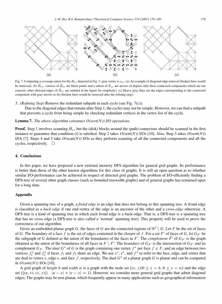
We define a connector pair coverage cycle as a simple cycle between two (path) connectors (examples are shownin Fig. 6(a)–(c)). Also, we define a coverage union as a union of connector pair coverage cycles such that all (path)connectors belong to the union.

We compute a path compensator PI I as follows:

1. Compute a coverage union (heavy lines in Fig. 6(d)).This step is described in Section 3.5. This step requires O(sort(N )) I/Os from Lemma 7.

2. Create a simple cycle C I I by taking the symmetric difference of all the cycles in the coverage union (Fig. 6(e)).This is done by removing the common edges among the cycles. This requires O(scan(N )) I/Os.

3. Find a simple path Pxy from sxy(or uxy) to some vertex in C I I (Fig. 6(f)).This can be done with O(sort(|V (Hxy)| + |E(Hxy)|)) = O(sort(N )) I/Os since vertex cardinality of Hxy is largerthan 2

3 |V | and this operation is similar to Step 2 of Planar DFS.4. Extend Pxy to a path PI I containing all the vertices in Pxy and C I I (Fig. 6(f)).

This requires O(scan(|V (Hxy)| + |E(Hxy)|)) = O(sort(N )) I/Os since this operation is similar to Step 3 ofPlanar DFS.

The overall I/O-complexity is O(sort(N )).

Lemma 6. The path PI I computed by the above algorithm is simple and is a compensator of C.

178 J.-H. Her, R.S. Ramakrishna / Theoretical Computer Science 374 (2007) 170–180

Fig. 6. Computing a path compensator PI I for the Hxy depicted in Fig. 3: gray vertex is sxy . (a), (b), and (c) represent three connector paircoverage cycles (heavy lines). (d) A coverage union (broken lines are shared edges among the connector pair coverage cycles). (e) A cycle aftertaking symmetric difference among the cycles. (f) After Step 3 and 4 (dotted line is removed for final PI I ).

Proof. We can consider each (path) connector as a vertex using edge contraction and the resulting graph is stillbiconnected. From Whitney’s characterization [24] of k-connected graphs, for each vertex pair, there is at least onecycle. Hence, for each (path) connector pair, there exists at least one connector pair coverage cycle. C I I is a simplecycle because it is built iteratively by taking the symmetric difference of two adjacent cycles and the two cyclesshare at least one (connector) edge. Thus, PI I is simple. Since two adjacent cycles meet at at least one end-vertexof a connector (or one terminal vertex of a path connector) due to the first condition of the ‘edge removal’ step inSection 3.5, C I I includes at least one end-vertex of each connector (or one terminal vertex of each path connector).Thus, PI I is a path compensator of C by definition. �

3.5. Computing a coverage union

Again, we exploit a section of the face identification scheme of Hutchinson et al. to compute a coverage unionI/O-efficiently. We compute a coverage union of the biconnected component Hxy = (Vxy, Exy) as follows:

1. (Preprocessing Step) Remove edges from intersecting diagonal edge pairs subject to the following two conditions:(i) one end (terminal) vertex of a (path) connector has degree at least three and (ii) every other vertex has at leastdegree two (to retain biconnectivity). Refer to Fig. 7(a) for an example.

2. Compute a directed graph Hxy = (Vxy, Exy) (see Fig. 7(b)).

A. For each edge {u, v} ∈ Exy , add two vertices v(u,v) and v(v,u) to Vxy .B. For each vertex u ∈ Vxy , sort its incident edges in counterclockwise order (let these sorted edges be

{u, v0}, . . . , {u, vl−1}).C. Add directed edges (v(vi ,u), v(u,v(i+1) mod l )) to Exy , 0 ≤ i < l.

3. Compute the connected components of Hxy that are related to the connectors (by considering the edges of Hxy asbeing undirected). Refer to Fig. 7(b) for an example.

4. Compute the cycles of Hxy which correspond to the connected components of step 3 (See Fig. 7(c)).

J.-H. Her, R.S. Ramakrishna / Theoretical Computer Science 374 (2007) 170–180 179

Fig. 7. Computing a coverage union for the Hxy depicted in Fig. 3: gray vertex is sxy . (a) An example of diagonal edge removal (broken lines wouldbe removed). (b) Hxy : vertices of Hxy are black points and a subset of Exy are arrows (it depicts only three connected components which are ourconcern; other directed edges of Hxy are omitted in the figure for simplicity). (c) Heavy gray lines are the edges corresponding to the connectedcomponent with gray arrows in (b) (broken lines would be removed after the refining step).

5. (Refining Step) Remove the redundant subpath in each cycle (see Fig. 7(c)).Due to the diagonal edges that remain after Step 1, the cycles may not be simple. However, we can find a subpath

that prevents a cycle from being simple by checking redundant vertices in the vertex list of the cycle.

Lemma 7. The above algorithm consumes O(sort(N)) I/O operations.

Proof. Step 1 involves scanning Hxy but the (disk) blocks around the (path) connectors should be scanned in the firstinstance to guarantee that condition (i) is satisfied. Step 2 takes O(sort(N )) I/Os [10]. Also, Step 3 takes O(sort(N ))I/Os [7]. Steps 4 and 5 take O(scan(N )) I/Os as they perform scanning of all the connected components and all thecycles, respectively. �

4. Conclusions

In this paper, we have proposed a new external memory DFS algorithm for general grid graphs. Its performanceis better than those of the other known algorithms for this class of graphs. It is still an open question as to whethersimilar I/O-performance can be achieved in respect of directed grid graphs. The problem of I/O-efficiently finding aDFS-tree of several other graph classes (such as bounded treewidth graphs) and of general graphs has remained openfor a long time.

Appendix

Given a spanning tree of a graph, a frond edge is an edge that does not belong to this spanning tree. A frond edgeis classified as a back-edge if one end-vertex of the edge is an ancestor of the other and a cross-edge otherwise. ADFS-tree is a kind of spanning tree in which each frond edge is a back-edge. That is, a DFS-tree is a spanning treethat has no cross edge (a DFS-tree is also called a ‘normal’ spanning tree). This property will be used to prove thecorrectness of our algorithm.

Given an embedded planar graph G, the faces of G are the connected regions of <2\ G. Let F be the set of faces

of G. The boundary of a face f is the set of edges contained in the closure of f . For a set F ′ of faces of G, let G F ′ bethe subgraph of G defined as the union of the boundaries of the faces in F ′. The complement F ′ of G F ′ is the graphobtained as the union of the boundaries of all faces in F \ F ′. The boundary of G F ′ is the intersection of G F ′ and itscomplement G F ′ . The dual G∗ of G is the graph containing one vertex f ∗ per face f ∈ F , and an edge between twovertices f ∗

1 and f ∗

2 if faces f1 and f2 share an edge. We use v∗, e∗, and f ∗ to refer to the face, edge, and vertex thatare dual to vertex v, edge e, and face f , respectively. The dual G∗ of a planar graph G is planar and can be computedin O(sort(N )) I/Os [10].

A grid graph of height h and width w is a graph with the node set {(x, y)|0 ≤ x < h, 0 ≤ y < w} and the edgeset {{(u, v), (x, y)}| |u − x | + |v − y| = 1}. However, we consider more general grid graphs that admit diagonaledges; The graphs may be non-planar, which frequently appear in many applications such as geographical information

180 J.-H. Her, R.S. Ramakrishna / Theoretical Computer Science 374 (2007) 170–180

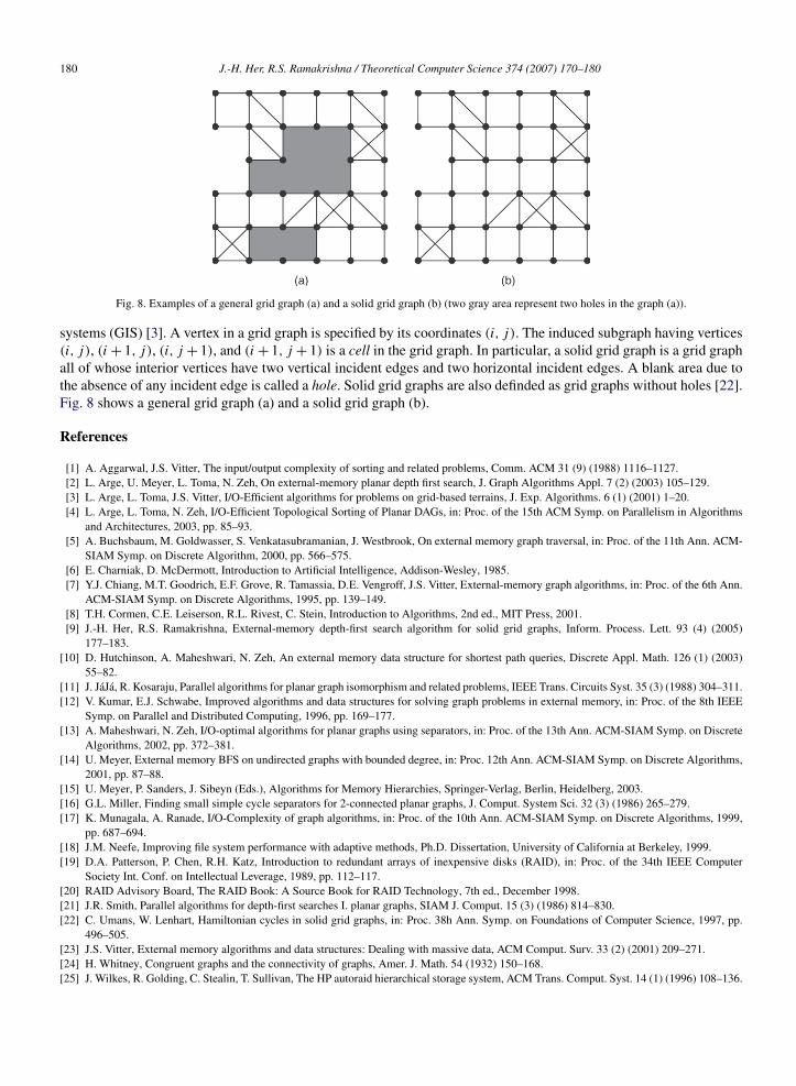
Fig. 8. Examples of a general grid graph (a) and a solid grid graph (b) (two gray area represent two holes in the graph (a)).

systems (GIS) [3]. A vertex in a grid graph is specified by its coordinates (i, j). The induced subgraph having vertices(i, j), (i + 1, j), (i, j + 1), and (i + 1, j + 1) is a cell in the grid graph. In particular, a solid grid graph is a grid graphall of whose interior vertices have two vertical incident edges and two horizontal incident edges. A blank area due tothe absence of any incident edge is called a hole. Solid grid graphs are also definded as grid graphs without holes [22].Fig. 8 shows a general grid graph (a) and a solid grid graph (b).

References

[1] A. Aggarwal, J.S. Vitter, The input/output complexity of sorting and related problems, Comm. ACM 31 (9) (1988) 1116–1127.[2] L. Arge, U. Meyer, L. Toma, N. Zeh, On external-memory planar depth first search, J. Graph Algorithms Appl. 7 (2) (2003) 105–129.[3] L. Arge, L. Toma, J.S. Vitter, I/O-Efficient algorithms for problems on grid-based terrains, J. Exp. Algorithms. 6 (1) (2001) 1–20.[4] L. Arge, L. Toma, N. Zeh, I/O-Efficient Topological Sorting of Planar DAGs, in: Proc. of the 15th ACM Symp. on Parallelism in Algorithms

and Architectures, 2003, pp. 85–93.[5] A. Buchsbaum, M. Goldwasser, S. Venkatasubramanian, J. Westbrook, On external memory graph traversal, in: Proc. of the 11th Ann. ACM-

SIAM Symp. on Discrete Algorithm, 2000, pp. 566–575.[6] E. Charniak, D. McDermott, Introduction to Artificial Intelligence, Addison-Wesley, 1985.[7] Y.J. Chiang, M.T. Goodrich, E.F. Grove, R. Tamassia, D.E. Vengroff, J.S. Vitter, External-memory graph algorithms, in: Proc. of the 6th Ann.

ACM-SIAM Symp. on Discrete Algorithms, 1995, pp. 139–149.[8] T.H. Cormen, C.E. Leiserson, R.L. Rivest, C. Stein, Introduction to Algorithms, 2nd ed., MIT Press, 2001.[9] J.-H. Her, R.S. Ramakrishna, External-memory depth-first search algorithm for solid grid graphs, Inform. Process. Lett. 93 (4) (2005)

177–183.[10] D. Hutchinson, A. Maheshwari, N. Zeh, An external memory data structure for shortest path queries, Discrete Appl. Math. 126 (1) (2003)

55–82.[11] J. JaJa, R. Kosaraju, Parallel algorithms for planar graph isomorphism and related problems, IEEE Trans. Circuits Syst. 35 (3) (1988) 304–311.[12] V. Kumar, E.J. Schwabe, Improved algorithms and data structures for solving graph problems in external memory, in: Proc. of the 8th IEEE

Symp. on Parallel and Distributed Computing, 1996, pp. 169–177.[13] A. Maheshwari, N. Zeh, I/O-optimal algorithms for planar graphs using separators, in: Proc. of the 13th Ann. ACM-SIAM Symp. on Discrete

Algorithms, 2002, pp. 372–381.[14] U. Meyer, External memory BFS on undirected graphs with bounded degree, in: Proc. 12th Ann. ACM-SIAM Symp. on Discrete Algorithms,

2001, pp. 87–88.[15] U. Meyer, P. Sanders, J. Sibeyn (Eds.), Algorithms for Memory Hierarchies, Springer-Verlag, Berlin, Heidelberg, 2003.[16] G.L. Miller, Finding small simple cycle separators for 2-connected planar graphs, J. Comput. System Sci. 32 (3) (1986) 265–279.[17] K. Munagala, A. Ranade, I/O-Complexity of graph algorithms, in: Proc. of the 10th Ann. ACM-SIAM Symp. on Discrete Algorithms, 1999,

pp. 687–694.[18] J.M. Neefe, Improving file system performance with adaptive methods, Ph.D. Dissertation, University of California at Berkeley, 1999.[19] D.A. Patterson, P. Chen, R.H. Katz, Introduction to redundant arrays of inexpensive disks (RAID), in: Proc. of the 34th IEEE Computer

Society Int. Conf. on Intellectual Leverage, 1989, pp. 112–117.[20] RAID Advisory Board, The RAID Book: A Source Book for RAID Technology, 7th ed., December 1998.[21] J.R. Smith, Parallel algorithms for depth-first searches I. planar graphs, SIAM J. Comput. 15 (3) (1986) 814–830.[22] C. Umans, W. Lenhart, Hamiltonian cycles in solid grid graphs, in: Proc. 38h Ann. Symp. on Foundations of Computer Science, 1997, pp.

496–505.[23] J.S. Vitter, External memory algorithms and data structures: Dealing with massive data, ACM Comput. Surv. 33 (2) (2001) 209–271.[24] H. Whitney, Congruent graphs and the connectivity of graphs, Amer. J. Math. 54 (1932) 150–168.[25] J. Wilkes, R. Golding, C. Stealin, T. Sullivan, The HP autoraid hierarchical storage system, ACM Trans. Comput. Syst. 14 (1) (1996) 108–136.