HAL Id: hal-00545286https://hal.archives-ouvertes.fr/hal-00545286

Submitted on 10 Dec 2010

HAL is a multi-disciplinary open accessarchive for the deposit and dissemination of sci-entific research documents, whether they are pub-lished or not. The documents may come fromteaching and research institutions in France orabroad, or from public or private research centers.

L’archive ouverte pluridisciplinaire HAL, estdestinée au dépôt et à la diffusion de documentsscientifiques de niveau recherche, publiés ou non,émanant des établissements d’enseignement et derecherche français ou étrangers, des laboratoirespublics ou privés.

An extension of the Bus asteroid taxonomy into thenear-infrared

Francesca E. Demeo, Richard P. Binzel, Stephen M. Slivan, Schelte J. Bus

To cite this version:Francesca E. Demeo, Richard P. Binzel, Stephen M. Slivan, Schelte J. Bus. An extensionof the Bus asteroid taxonomy into the near-infrared. Icarus, Elsevier, 2009, 202 (1), pp.160.�10.1016/j.icarus.2009.02.005�. �hal-00545286�

Accepted Manuscript

An extension of the Bus asteroid taxonomy into the near-infrared

Francesca E. DeMeo, Richard P. Binzel, Stephen M. Slivan, SchelteJ. Bus

PII: S0019-1035(09)00055-4DOI: 10.1016/j.icarus.2009.02.005Reference: YICAR 8908

To appear in: Icarus

Received date: 30 October 2008Revised date: 6 February 2009Accepted date: 9 February 2009

Please cite this article as: F.E. DeMeo, R.P. Binzel, S.M. Slivan, S.J. Bus, An extension of the Busasteroid taxonomy into the near-infrared, Icarus (2009), doi: 10.1016/j.icarus.2009.02.005

This is a PDF file of an unedited manuscript that has been accepted for publication. As a service toour customers we are providing this early version of the manuscript. The manuscript will undergocopyediting, typesetting, and review of the resulting proof before it is published in its final form. Pleasenote that during the production process errors may be discovered which could affect the content, and alllegal disclaimers that apply to the journal pertain.

ACCEP

TED M

ANUSC

RIPT

ACCEPTED MANUSCRIPT

An extension of the Bus asteroid taxonomy into

the Near-Infrared

Francesca E. DeMeo a, Richard P. Binzel b, Stephen M. Slivan b,

and Schelte J. Bus c

aLESIA, Observatoire de Paris, F-92195 Meudon Principal Cedex, France

bDepartment of Earth, Atmospheric, and Planetary Sciences, Massachusetts Insti-

tute of Technology, Cambridge, MA 02139

cInstitute for Astronomy, 640 N. Aohoku Place, Hilo, HI 96720

Number of pages: 65

Number of tables: 5

Number of figures: 15

Number of appendices: 4

1

ACCEP

TED M

ANUSC

RIPT

ACCEPTED MANUSCRIPT

Proposed Running Head: An extension of the Bus asteroid taxonomy into the

Near-Infrared

Please send Editorial Correspondence to: Francesca E. DeMeo

LESIA, Observatoire de Paris

F-92195 Meudon Principal Cedex, France

Email: francesca.demeo@obspm.fr

Phone: +33 1 45 07 74 09

Fax: +33 1 45 07 71 44

2

ACCEP

TED M

ANUSC

RIPT

ACCEPTED MANUSCRIPT

ABSTRACT

The availability of asteroid spectral measurements extending to the near-infrared,

resulting from the development of new telescopic instruments (such as SpeX; Rayner

2003), provides a new basis for classifying asteroid reflectance spectra. We present

an asteroid taxonomy classification system based on reflectance spectrum charac-

teristics for 371 asteroids measured over the wavelength range 0.45 to 2.45 microns.

This system of 24 classes is constructed using principal component analysis, fol-

lowing most closely the visible wavelength taxonomy of Bus (1999), which itself

builds upon the system of Tholen (1984). Nearly all of the Bus taxonomy classes

are preserved, with one new class (Sv) defined. For each class we present boundary

definitions, spectral descriptions, and prototype examples. A flow chart method is

presented for classifying newly acquired data spanning this wavelength range. When

data are available only in the near-infrared range (0.85 to 2.45 microns), classifica-

tion is also possible in many cases through an alternate flow chart process. Within

our sample, several classes remain relatively rare: only 6 objects fall into

the A-class; 349 Dembowska and 3628 Boznemcova reside as the only

objects in their respective R- and O-classes. Eight Q-class objects are all

near-Earth asteroids. We note 1904 Massevitch as an outer main-belt V-

type while 15 other V-type objects have inner main-belt orbits consistent

with an association with Vesta.

Keywords:ASTEROIDS; SPECTROSCOPY

3

ACCEP

TED M

ANUSC

RIPT

ACCEPTED MANUSCRIPT

1 Introduction

Taxonomic classification systems for asteroids have existed since there were enough

data to distinguish meaningful groups. The first taxonomies were based on aster-

oid broad band filter colors such as Wood and Kuiper (1963) and Chapman et al.

(1971) where they noted two separate types of objects denoted as “S” and “C”.

Taxonomies and their nomenclature grew and evolved as later taxonomies became

based on higher resolution spectral data which reveal features offering clues to sur-

face composition, age, and alteration. The most widely used taxonomies for asteroids

currently are the Tholen taxonomy (1984) based on the Eight-Color Asteroid Sur-

vey data (ECAS, Zellner et al., 1985) and SMASSII spectral taxonomy (Bus, 1999;

Bus and Binzel, 2002a,b) based on the SMASSII spectral dataset. For a review of

the evolution of asteroid taxonomies see Bus (1999).

Both the Tholen and Bus taxonomies were based on Principal Component Analysis,

a dimension-reducing technique first applied to the field of asteroid classification

by Tholen (1984). Most previous asteroid taxonomies were based on visible data be-

cause only in the current decade has spectral data collection become widely available

in the near-infrared for asteroids down to relatively faint (V=17) limiting magni-

tudes. The instrument SpeX on the NASA Infrared Telescope Facility (IRTF) has

been crucial to increasing the library of near-IR asteroid spectra. (Rayner et al.,

2003)

The near-IR data range reveals diagnostic compositional information because of

the presence of features at one and two microns primarily due to the presence of

olivine and pyroxene. Other classification systems created using near-IR data in-

clude Howell et al. (1994) who created a neural network taxonomy. Gaffey

et al. (1993) created an S-complex taxonomy of olivine- and pyroxine-rich asteroids

based on near-infrared data. Our goal was to create a taxonomy extending from

4

ACCEP

TED M

ANUSC

RIPT

ACCEPTED MANUSCRIPT

visible to near-infrared wavelengths for the entire suite of asteroid characteristics

with a method that can be easily reproduced by future users to classify new data.

We also strove to keep the notation consistent with past taxonomies, specifically the

Bus taxonomy, to facilitate the transition to this new system. The Bus taxonomy,

in turn, strove to keep its notation consistent with the Tholen taxonomy.

The taxonomy we present here is based on Principal Component Analysis. It is

comprised of 24 classes compared to 26 in the Bus system with three Bus classes

eliminated (Sl, Sk, Ld) and one (Sv) created, as well as the addition of a “w”

notation, a mark meant to flag objects having similar spectral features but differing

only by having a higher spectral slope. In this paper we present the data involved in

the taxonomy and the method and rationale for the class definitions. The taxonomy

classes are formally defined by data spanning the wavelength range 0.45 to 2.45

microns as compared with 0.34 to 1.04 microns for Tholen (1984) using eight points,

and 0.435 to 0.925 microns for Bus (1999) using 48 points. A method of interpreting

near-infrared data from 0.85 to 2.45 microns is also described but for many classes

IR-only data do not yield a unique outcome in Principal Component Analysis (PCA)

and the data cannot formally be classified. There is also a web application that

determines taxonomic types for visible plus near-infrared data or near-infrared-only

data based on this extended taxonomy. (http://smass.mit.edu/busdemeoclass.html)

5

ACCEP

TED M

ANUSC

RIPT

ACCEPTED MANUSCRIPT

2 The Data

New data presented here are near-infrared spectral measurements from 0.8 to 2.5

microns obtained using SpeX, the low- to medium- resolution near-IR spectrograph

and imager (Rayner et al., 2003), on the 3-meter NASA IRTF located on Mauna

Kea, Hawaii. As described in DeMeo and Binzel (2008), objects and standard stars

were observed near the meridian to minimize their differences in airmass and match

their parallactic angle to the fixed N/S alignment of the slit. Frames were taken

so that the object was alternated between two different positions (usually noted

as the A and B positions) on a 0.8 x 15 arcsecond slit aligned north-south. The

asteroid spectrum was divided by the spectrum of a solar-type star, giv-

ing relative reflectance. Our primary solar analog standard stars were 16 Cyg

B and Hyades 64. Additional solar analog stars with comparable spectral

characteristics were utilized around the sky. Two to three sets of eight spectra

per set were taken for each object, with each with exposures typically

being 120 seconds. The total integration time for each of these objects therefore

ranged from 30 to 120 minutes.

6

ACCEP

TED M

ANUSC

RIPT

ACCEPTED MANUSCRIPT

Reduction was performed using a combination of routines within the Image Reduc-

tion and Analysis Facility (IRAF), provided by the National Optical Astronomy

Observatories (NOAO) (Tody, 1993), and Interactive Data Language (IDL). We

use a software tool called “autospex” to streamline reduction procedures. Autospex

writes macros containing a set of IRAF (or IDL) command files that are then ex-

ecuted by the image processing package. Autospex procedures operate on a single

night at a time, with the opportunity for the user to inspect and verify the results

at each stage. Briefly, autospex writes macros that: trim the images down to their

useful area, create a bad pixel map from flat field images, flat field correct all images,

perform the sky subtraction between AB image pairs, register the spectra in both

the wavelength and spatial dimensions, co-add the spectral images for individual

objects, extract the 2-D spectra from co-added images, and then apply the final

wavelength calibration. Using IDL, an absorption coefficient based on the atmo-

spheric transmission (ATRAN) model by Lord (1992) is determined for each object

and star pair that best minimizes atmospheric water absorption effects for that pair.

This coefficient correction is most important near 1.4 and 2.0 microns, locations of

major absorption bands due to telluric H2O. The final IDL step averages all the

object and standard pairs to create the final reflectance spectrum for each object.

Most (321) visible wavelength spectra (usually 0.4 to 0.9 microns) were taken from

the Small Main Belt Asteroid Spectroscopic Survey (SMASS II) data set (Bus and

Binzel, 2002a). Our sample was comprised of 371 objects with both visible and near-

IR data. For a table of observations and references for all data included in

this work as well as the final taxonomic designations for all objects see

Appendix A. The spectra are plotted in Appendix D.

7

ACCEP

TED M

ANUSC

RIPT

ACCEPTED MANUSCRIPT

3 Creating the Taxonomy

Principal Component Analysis (PCA) is a method of reducing the dimen-

sionality of a data set, involving coordinate transformations to minimize

the variance. The first transformation rotates the data to maximize vari-

ance along the first axis, known as Principal Component 1 (PC1′), the

second axis is the second Principal Component (PC2′). The first few prin-

cipal components contain the majority of the information. For a more

thorough explanation of PCA and why it is useful for asteroid taxonomy

refer to Tholen (1984) and Bus (1999).

3.1 Data Preparation

To prepare our data, we created spline fits to our spectra which smoothed the

spectra creating a best fit curve. This reduced the risk that noise or missing data

points would influence the resulting taxonomy. We sampled the region 0.45 to 2.45

microns and recorded values of the spline fit at increments of 0.05 microns resulting

in 41 datapoints.

The splined data were then normalized at 0.55 microns and the slope was removed

from the data and recorded. Using our normalized data, we took a linear

regression line of each set of data. The slope (γ) of the linear regression line is

defined by Eq. 1:

γ =∑i

0(xi − x)(yi − y)∑i

0(xi − x)2(1)

where xi is each wavelength value, yi is each fitted reflectance, and x and y are their

mean values. We note the slope is not constrained to pass through 1 at

8

ACCEP

TED M

ANUSC

RIPT

ACCEPTED MANUSCRIPT

0.55 microns. The calculated slope is thus independent of one’s choice

for the wavelength at which a spectrum is normalized. The equation of

the line defining the slope is then translated in the y-direction to pass

through 1 at 0.55 microns.

(equation removed)

Because slope is the most prominent feature of the spectra we remove it from the

data by dividing the slope function, before performing principal component analysis

thus making PCA more sensitive to other features. We divide all the data points

by the fitted slope. The remaining data are a spectrum with an average slope

of zero residuals (including absorption features) above and below the horizontal.

We now have data with 41 channels normalized to unity at 0.55 microns with the

slope removed. Because each spectrum has a value of 1 at 0.55μm, that channel

provides no new information and so was removed from the data set to make PCA

more effective. Therefore we input 40 channels per object into PCA. Us-

ing MATLAB, we then performed PCA on the splined files with slopes

removed. We chose to use covariance instead of correlation for the PCA

implementation as suggested by Bus (1999).

Following the method of Bus (1999), we verify the slope as a constant signal within

all data. Figure 1 displays the first principal component (PC1) of PCA before re-

moving slope compared to the slope we remove directly from the splined data. In the

figure it is clear that the two are linearly correlated, justifying the value of removing

slope and tabulating it as a spectral parameter.

[Fig. 1: PC1 versus Slope]

9

ACCEP

TED M

ANUSC

RIPT

ACCEPTED MANUSCRIPT

3.2 Notation

Here we offer a note on our notation: we use the “ ′ ” notation to denote that

principal component analysis is performed on data from which the slope has been

removed. Thus PC1′ is the first principal component of asteroid data that has

already had its slope removed. To perform PCA the average value for each

channel is subtracted from the data set, resulting in a data set with

mean for each channel equal to zero. Note that this notation differs from the

Bus (Bus, 1999; Bus and Binzel, 2002b) notation in which the first principal

component that has already had its slope removed is PC2′. The supplementary

material provides a table of the eigenvalues for the first five principal components

and the mean value for each channel. To compute the principal components of a

data set, the transpose of the eigenvector is multiplied by the transpose of the

mean-subtracted data set as described in Eq. 2:

PCx = [ETx ][DT ] (2)

where PCx is principal component x, Ex is eigenvector x. D is the column vector

containing an individual reflectance spectrum, normalized to unity at 0.55 μm,

from which the mean channel value (see supplementary material) has been

subtracted at each wavelength.

3.3 Choosing the Number of Principal Components

Bus (Bus, 1999; Bus and Binzel, 2002b) used slope plus two principal com-

ponents to characterize visible data contained in 48 wavelength channels. Because

40 wavelength channels were put into our PCA, 40 principal components were the

output. Since PCA concentrates the most information in the first dimensions, and

10

ACCEP

TED M

ANUSC

RIPT

ACCEPTED MANUSCRIPT

decreases with each successive dimension, only the first few principal components

are useful. To decide how many principal components to use in our analysis we look

at the variance contained within each.

The first five principal components contain 99.2% of the variance, which

is sufficient to describe these spectra. PC4′ and PC5′ were found to be

useful for classifying the subtly featured X- and C-complex objects. To

find the variance contained within the slope we ran PCA with the slope

included in the data. Slope accounts for 88.4% of all the variance within the data.

All the other principal components combined account for 11.6%. Thus, Slope plus

the first five PC account for 99.9% of the variance. Table 1 shows the variances

accounted for by the slope and each of the first five principal components.

(scree plot figure removed)

[Table 1: Variance within Principal Components]

4 The Taxonomy

Of the 371 objects in our sample, 321 were previously assigned labels within the

Bus taxonomy. We used this set of 321 objects to guide the class boundaries. The

following describes the separation of complexes and classes and the resultant flow

chart to reproduce these results using any dataset. Our method is similar to that of

Bus (Bus, 1999; Bus and Binzel, 2002a,b); we start by defining the end mem-

bers, and then move to define the core of each complex. The three main complexes

are consistent with past taxonomies: the S-complex displays strong absorptions at 1

and 2μm, the C-complex shows low to medium slope and either small or no features,

and the X-complex has medium to high slope also displays either small or no fea-

11

ACCEP

TED M

ANUSC

RIPT

ACCEPTED MANUSCRIPT

tures. The complexes are meant to group classes that show similar characteristics.

The end member classes are more distinct and separate farther from other types

among their principal components. For all the new classifications of the 371 objects

in our dataset see Appendix B.

4.1 The Grand Divide

The most striking feature seen within the principal component space is the large

gap in PC1′ versus PC2′ space seen in Fig. 2. It appears that this clear boundary

distinguishes between spectra that have a 2-μm absorption band and those that do

not. This “grand divide” is well represented by Eq. 3:

PC1′ = −3.00PC2′ − 0.28 (line α) (3)

This “grand divide” is a natural boundary revealed by the principal component

analysis that relates PC1′ and PC2′. While no other boundary in this taxonomy

is as distinct and well-defined, we used this natural divide as a guide for other, more

artificially created boundaries. When defining classes to the right of line α, we used

lines parallel and orthogonal to it to carve out the space. Fig. 2 , 3 and 4 plot all

objects in PC1′ and PC2′ space. Fig. 2 shows all objects. Fig. 3 shows only objects

right of line α plus the A- and Sa-types with the boundaries and line labels that

carve out this space. Fig. 4 shows objects left of line α except A- and Sa-types. It

is clear from Fig. 4 that the C- and X-complexes do not separate clearly in this PC

space. For plots showing the placement of objects in this sample with their Bus,

Tholen, and Gaffey labels, see the Supplementary Material.

[Fig. 2: Main plot of all objects in PC2′ v PC1′ Space]

[Fig. 3: Main plot of all “featured” objects in PC2′ v PC1′ Space]

12

ACCEP

TED M

ANUSC

RIPT

ACCEPTED MANUSCRIPT

[Fig. 4: Main plot of all “subtly featureled” objects in PC2′ v PC1′ Space]

Except for some L-class objects at the top left of Fig. 2, all objects below and to the

left of line α have no two-micron absorption feature and include all subtly featured

(C- and X-complex) spectra. By “subtly featured” we mean there may or may

not be shallow absorption features particularly in the visible wavelength

range, however, there are no prominent one or two-micron absorption bands.

Objects plotted to the right of and above the line have a two-micron absorption

feature. The only classes that cross this gap are the A- and Sa-classes. Interestingly

the K-class, long considered as an intermediate between S and C, falls most squarely

in the gap.

While there is no predefined key to understanding the significance of each principal

component in separating different spectral types, looking at how the gradient of

spectra is distributed in Fig. 2 helps us decipher what effect each principal compo-

nent has. For objects to the right of line α, moving parallel to the line in

the decreasing PC1′ direction corresponds to increasing 1-micron band

depth and width. Moving perpendicular to the line in the increasing

PC2′ direction (to the right) corresponds to increasing depth and width

of the 2-micron band. The C- and X-complexes have subtler features,

and thus have lower PC2′ values while S-complex objects have greater values

and strongly featured end members such as V- and R-classes plot furthest to the

right with the largest PC2′ values. As PC1′ values decrease (moving from top to

bottom on Fig. 2) the one-micron band becomes broader and in general deeper.

The narrow one-micron band V- types plot on the top right with wide Q- and even

wider Sa- and A -types toward the bottom left. Types A, Q, and R with deeper

bands all plot below the less extreme S-complex transition types, Sa, Sq, and Sr.

The guiding principle for the classification rules of this taxonomy was to define re-

13

ACCEP

TED M

ANUSC

RIPT

ACCEPTED MANUSCRIPT

gions of principal component space that most consistently envelop objects within

each of the original Bus (1999) classes. With this principle as a guide, we sub-

jectively define boundaries so that the most similar spectra consistently

fall into the same taxonomic classes. As discussed below, the over-riding cri-

terion of similarity of spectral properties in a class, as examined over the full 0.45

- 2.45 μm range, led to some objects in the Bus (Bus, 1999; Bus and Binzel,

2002b) classification receiving new class designations here.

To assign classes for the taxonomy we created a flowchart (Appendix B)

containing steps to find a the taxonomic class that results in a consistent

grouping of objects with similar spectral properties. The labels for each class

follow, except where noted, the same label as Bus (Bus, 1999; Bus and Binzel,

2002b). The order of the flow chart is significant because some classes overlap in

certain principal components but can be separated in others.

We start by separating the A- and Sa-classes because they cross over the “grand

divide” in PC1′ and PC2′ space. This is step 1 in the flow chart. Refer to Appendix

B for the complete chart. Spectrally, the A-class has a deep and extremely broad

absorption band with a minimum near 1 μm and may or may not have shallow 2-

μm absorption band; it also tends to be steeply sloped. The Sa-class has the same

characteristic 1-μm absorption band as the A-class, but is less red.

The current Sa-class was redefined from the Bus system because the two Sa objects

(main belt object 984 Gretia and Mars crosser 5261 Eureka) in this system

were both Sr-types in the Bus system. Since these objects prove to be intermediate

between S and A we change the classification of these two (Bus) Sr-types to Sa in

this taxonomy. Figure 5 shows the spectral progression from S to A.

[Fig. 5: Plot of S, Sa, and A spectra]

Step two starts by separating all objects by the divide (line α) in PC2′ versus

14

ACCEP

TED M

ANUSC

RIPT

ACCEPTED MANUSCRIPT

PC1′ space, and creates boundaries for objects with a two-micron band. Step three

addresses subtly featured objects (the C- and X-complexes) as well as the K-class

which has no significant two-micron band and the L-class which may or may not

have a two-micron absorption band but nonetheless lies to the left of line α.

4.2 The End Members: O, Q, R, V

We started by looking at the end member classes in PCA space since they separate

most clearly, thereby making them the easiest to define. In Fig. 3 one can see lines

separating S-complex and end member classes. Equations 3, 4, 5, 6, and 7 bound

these classes.

PC1′ = −3.0PC1′ + 1.5 (line δ) (4)

PC1′ = −3.0PC1′ + 1.0 (line γ) (5)

PC1′ =13PC1′ − 0.5 (line η) (6)

PC1′ = −3.0PC1′ + 0.7 (line θ) (7)

The V-class, based on the asteroid 4 Vesta (Tholen 1984), is characterized by its

strong and very narrow 1-μm absorption band, as well as a strong and wider 2-

μm absorption feature. Most V-class asteroids that have been discovered are among

the Vesta family and are known as Vestoids, although a few other objects have

been identified throughout the main belt, such as 1459 Magnya (Lazzaro et al.,

2000) and objects from the basaltic asteroid survey by Moskovitz et al. (2008). The

R-class, created for its sole member 349 Demboska by Tholen (1984), is similar

to the V-class in that it displays deep 1- and 2-μm features, however the one-

micron feature is broader than the V-type feature and has a shape more

similar to an S-type except with deeper features. The R-class region in

15

ACCEP

TED M

ANUSC

RIPT

ACCEPTED MANUSCRIPT

principal component space is plotted in (Fig. 3). Bus (Bus and Binzel,

2002b)included three other members in the R-class, two of which are included in

our sample. These two objects (1904 Massevitch and 5111 Jacliff) were reassigned

to the V-class after discovering that in the near-infrared their one-micron bands

remain very narrow. Moskovitz et al. (2008) list 5111 Jacliff as an “R-

type interloper” within the Vesta family, but it appears to be an object

more confidently linked to Vesta. 1904 Massevitch, however, has a semi-

major axis of 2.74 AU. The unusual spectrum and outer belt location

for asteroid 1904 has been noted previously (e.g. Burbine and Binzel

(2002)). In the sample we present here, asteroids 1904 Massevitch and

1459 Magnya (Lazzaro et al., 2000) are the only two V-types beyond 2.5

AU, a region where V-type asteroids are rare (Binzel et al., 2006, 2007;

Moskovitz et al., 2008).

The O-class also has only one member, 3628 Boznemcova, defined by Binzel et al.

(1993). Boznemcova is unique with a very rounded and deep, bowl shape absorption

feature at 1-micron as well as a significant absorption feature at 2 μm. (boundary

line information removed) Even though the class is separated in the flow chart,

more data on R-type and O-type objects may help establish more rigorously

their region boundaries. Bus (Bus and Binzel, 2002b) designated three other

asteroids as O-type, 4341 Poseiden, 5143 Heracles, and 1997 RT. Only 5143 was in-

cluded in our sample. Asteroid 5143 is reclassified here as a Q-type because

with near-infrared data it is clear the object did not have the distinct ”bowl” shape

of the one-micron feature of Boznemcova. This adds 5143 Heracles as a Q-type

to those known within near-Earth space (e.g Binzel et al. (2004c)).

The Q-class, whose boundaries are labeled in Fig. 3 was first defined by Tholen

(1984) for near-Earth asteroid 1862 Apollo. The class is characterized by a deep and

distinct 1-μm absorption feature with evidence of another feature near 1.3 μm as

16

ACCEP

TED M

ANUSC

RIPT

ACCEPTED MANUSCRIPT

well as a 2-μm feature with varying depths among objects. The spectral differences

between the end member classes V, R, Q, and O are displayed in Fig. 6.

(figure removed)

[Fig. 6: Plot of V, O, Q, R spectra.]

4.3 The S-Complex: S, Sa, Sq, Sr, Sv

Just as in the case of the Bus taxonomy, the S-complex was by far the most

difficult to subdivide. Most Bus classes within the S-complex seemed to blend

together or scatter randomly in all combinations of PCA components. For example,

many objects labeled as “Sa” and “Sl” in the Bus (Bus, 1999; Bus and Binzel,

2002b) taxonomy no longer form distinct groups when their spectra are ex-

tended into the near-IR. Most original Bus class objects of these types merged into

the S-class. Sa objects were most easily distinguishable not by absorption features,

but by their greater slope (caused by slope increases in the 1- to 1.5-micron range).

Similarly, many Bus S, Sq, and Sk objects become less clearly separated when

their spectra extend to the near-infrared. Within PCA space, the Bus S, Sq, and Sk

objects were initially impossible to define clearly because the boundaries blur and

overlap. Because spectrally the main difference between the classes of the S-complex

appears to be the width of the 1-micron absorption band we used the wavelength

range 0.8 to 1.35 microns and performed PCA on only S-complex objects to gain

insight on their differences.

Once we used this S-class PCA as a guide, it became more clear how to separate

classes within PC1′ and PC2′. We continued to use boundaries parallel and perpen-

dicular to line α. Each class has its own region in PC2′ and PC1′ space. Fig. 3

shows the S-complex boxes labeled in PCA space. The previously defined equations

3, 5, 6, plus Eqs. 8, 9, and 10 bound the S-complex.

17

ACCEP

TED M

ANUSC

RIPT

ACCEPTED MANUSCRIPT

PC1′ = −3.0PC1′ + 0.35 (line β) (8)

PC1′ =13PC1′ − 0.10 (line ζ) (9)

PC1′ =13PC1′ + 0.55 (line ε) (10)

Objects that reside just below the S-class in Fig. 3 appear similar to Q-types,

but with more shallow absorption bands. These are Sq-types transitioning between

S and Q. Sr-types transition between S- and R-classes. One object (5379 Abehiroshi)

was a V-type under the Bus (Bus and Binzel, 2002b) system and is now labeled

an Sr. While the visible data have a “moderate to very steep UV slope shortward

of 0.7 μm with a sharp, extremely deep absorption band longward of 0.75 μm”

(Bus and Binzel, 2002b), it is clear with the inclusion of near-infrared data that the

one-micron absorption band is too wide to be a V-type.

Two objects (2965 Surikov and 4451 Grieve) with high PC1′ values,

are considered spectrally unique from Sr because they exhibit very narrow 1-μm

absorption bands. The objects in this region spectrally appear to be in transition

between S- and V-classes. They are not included in the Bus dataset, and Bus and

Binzel (2002b) did not report any cases of objects with these characteristics.

Because of their intermediate properties between S and V that are clearly displayed

over the 0.45- to 2.45-micron range, we define a new class with the label Sv. Sk

objects in the Bus taxonomy are found to become diverse when the spectra extend

to near-IR wavelengths. All of these objects fall into other defined categories. Thus

the Sk class is excluded from this new system. Fig. 7 displays the spectra of

typical S-, Sq-, Sr-, and Sv-class spectra.

[Fig. 7: Plot of S-complex spectra (S, Sq, Sr, Sv).]

The objects in the S-complex had widely varying spectral slopes. To have some

taxonomic distinction in spectral characteristics arising from slope, we made an

18

ACCEP

TED M

ANUSC

RIPT

ACCEPTED MANUSCRIPT

arbitrary cutoff at Slope = 0.25 dividing high slope objects from other objects.

These objects are not relabeled in a class of their own. Instead the S, Sq, Sr, and Sv

objects with high slopes receive a notation of w added to their name as a moniker for

what is commonly discussed as an increase in slope arising from space weathering

(Clark et al., 2002). [We make no pretense of knowing whether or not their surfaces

are actually weathered.] The high slope S objects are labeled Sw, Sqw, Srw and

Svw. We extended this flag to the V- types for which there were two

objects with slopes greater than 0.25, which we label as Vw. Sa-types do

not receive a w notation because, as an intermediate class between S and A, they

are by definition highly sloped. Fig. 8 displays the differences between low- and

high-slope objects, S and Sw.

[Fig. 8: S versus Sw Spectra]

The choice of 0.25 for the “w” notation is arbitrary. When plotting Bus labeled

S, Sa, and Sl objects, there is a mixing around the 0.23 to 0.27 slope range. The

goal was to keep the “w” notation more selective without setting the boundary too

high where objects with unusual slope features (such as deeper UV dropoffs) were

preferentially selected rather than focusing on the significant slope range between

one and two microns for the S-Complex. Figure 9 plots Slope versus PC1′, showing

the line separating “w” objects from regular objects.

[Fig. 9: Separation between S and Sw in PC space]

4.4 The End Members: D, K, L, T

Step three focuses on objects below or to the left of line α (Eq. 3). We again start

by removing end members. Bus (Bus and Binzel, 2002b) objects in the D- and

T-classes continue to be easily separated by their high slopes and PC1′, PC2′, and

19

ACCEP

TED M

ANUSC

RIPT

ACCEPTED MANUSCRIPT

PC3′ values. D-types have spectra that are linear with very steep slope (greater

than 0.38), and some show slight curvature or a gentle kink around 1.5 μm. We

note that some objects have their classification most strongly driven by

their slope. It is possible for an object in the high-sloped A-class to fall

very close to the A/D boundary (for example, the A-type 354 Eleonora).

For objects near this boundary, a simple inspection for the presence of a

1-μm absorption band eliminates any possible confusion, where a strong

1-μm band is a distinctive feature of all A-types. T-types are linear with

moderate to high slope (between 0.25 and 0.38) and often gently concaving

down. We separate out L objects based on PC2′ versus PC1′. For objects residing

in the L component space it is necessary to check for Xe-type objects. Xe is a class

defined in the Bus system that is generally featureless except for a distinct hook at

0.49 microns, a feature that is not recognized within the first five components of

PCA. By visually inspecting the spectrum, one can identify a feature at 0.49 and

an absence of a slight feature around 1 micron and label the object as an Xe instead

of an L. Refer to Fig. 10 of slope versus PC1′ which shows how D and L are fairly

distinct. The K-types can then be distinguished clearly in PC2′ and PC3′ space.

The Bus (Bus and Binzel, 2002b) L- and K-classes were part of the S-class

in the Tholen (1984) taxonomy. While the L-class may show one- and two-micron

features, it is distinct from the S-class because the steep slope in visible region levels

out abruptly around 0.7 μm, but does not show a distinct absorption band like the S.

There is often a gentle concave down curvature in the near-infrared with a maximum

around 1.5 μm, and there may or may not be a 2-micron absorption feature. A

typical K-class object displays a wide absorption band centered just longward of 1

μm. This feature is unique because the left maximum and the minimum are sharply

pointed and the walls of the absorption are linear with very little curvature. Fig.

11 plots typical spectra for the D-, L-, K-, T-, and X-classes.

20

ACCEP

TED M

ANUSC

RIPT

ACCEPTED MANUSCRIPT

We found that all Ld-type objects under the Bus system diverged into the separate

L- and D-classes when near-infrared data were added. Thus the Ld-class itself is not

necessary for distinguishing over the visible plus near-infrared wavelength range.

The Ld-class does not continue into this new taxonomy.

[Fig. 10: D and L in Slope v PC1′ space.]

[Fig. 11: Plot of typical D-, L-, K-, T-, and X-class Spectra]

4.5 The C- and X-Complexes: B, C, Cb, Cg, Cgh, Ch ; X, Xc, Xe, Xk

We now consider the core C- and X-complexes. The B-types are easily dis-

tinguished by their negative slope as well as negative PC1′ and PC4′ values. Their

spectra are linear and negatively sloping often with a slight round bump around 0.6

μm preceding a slight feature longward of 1 micron and/or a slightly con-

cave up curvature in the 1- to 2-μm region. The X-class can then be easily identified

based on high slope values between 0.2 and 0.38. At this point Xe and Xk objects

may be present in X-class PC space. Our PCA is not particularly sensitive

to the small Xk feature, therefore the spectrum must be visually inspected for

a slight feature present usually near 0.9 to 1 micron. If the feature is present,

the object is designated an Xk. Xc-types have low to medium slope and are slightly

curved and concave downward.

Ch objects have a small positive slope that begins around 1.1 microns and slightly

pronounced UV dropoff, and a broad, shallow absorption band centered near

0.7 μm. The Ch objects are well distinguished in PC1′ and PC4′ space, but a check

must be done to distinguish them from the Cgh-type. The Cgh-class is similar to

the Ch showing a 0.7-micron feature, but also has a more pronounced UV dropoff

like the Cg-type. The C- and Cb-types separate in PC1′, PC4′, and PC5′. Figures

21

ACCEP

TED M

ANUSC

RIPT

ACCEPTED MANUSCRIPT

12 and 13 show the C-complex plotted in PCA space. C-types are linear with

neutral visible slopes and often have a slight rough bump around 0.6 μm and low

but positive slope after 1.3 μm. Cb-types are linear with a small positive slope that

begins around 1.1 μm. Cb objects were intermediate objects between the B-

and C-classes in the Bus system (Bus and Binzel, 2002b). We keep the

same notation, however, the near-infrared data shows, that Cb objects

have low to moderate near-infrared slopes, while the visible slopes are low

or negative. There is only one object (175 Andromache) in the Cg-class carrying

over from the Bus (Bus, 1999; Bus and Binzel, 2002b) taxonomy. The Cg-class

is characterized by a pronounced UV dropoff similar to the Cgh, but does not show

the 0.7-micron feature that define Ch and Cgh. The classes Cg, Cgh, Ch, Xk, Xc,

and Xe do not all separate cleanly in component space because their distinguishing

features are weak and not well detected by the first five principal components. These

classes often must be distinguished by visually detecting features described by Bus

(1999). A summary of these features are described at the end of the flowchart,

Appendix B. Fig. 14 shows typical spectra for classes within the C- and

X-complexes.

[Fig. 12: C-Complex in PC5′ v PC1′ space.] [Fig. 13: C-Complex in PC4′ v PC1′

space.] [Fig. 14: Typical C- and X-complex spectra]

4.6 A Near-Infrared-Only Classification Method

For many objects, data exist in either the visible or near-infrared wavelength ranges

but not both. While taxonomies such as the Bus system (Bus, 1999; Bus and Binzel,

2002b) are available for visible data, no system has been widely accepted for assign-

ing classes to data existing only in the near-infrared. We have adapted our present

taxonomy to interpret spectral data available only in the near-infrared range. This

22

ACCEP

TED M

ANUSC

RIPT

ACCEPTED MANUSCRIPT

adaptive taxonomy is not meant to determine a definite class, but instead is an in-

termediate tool to indicate classes. We especially note that several classes in section

4.5 are carried over unchanged from the Bus taxonomy and are based exclusively on

features present at visible wavelengths. Assignment to these classes (Cg, Cgh,

Xc, Xe, Xk) requires visible wavelength data, therefore objects in these

classes cannot be recognized by near-infrared-only data.

To study the ability to classify objects having only near-infrared spectral

data we took the same 371 objects used in the original taxonomy but

included only data longward of 0.85 microns, again splining the data to

smooth out noise. Our spline increments remained 0.05 μm covering the range of

0.85 to 2.45 microns resulting in 33 datapoints. We chose to normalize to unity

at 1.2 microns, the closest splinefit wavelength value to 1.215 μm which

is the isophotal wavelength for the J band based on the UKIRT filter

set (Cohen et al., 1992). Next, we removed the slope from the data. As in the

case with visible and near-infrared data we calculated the slope function

without constraints, and then translate it in the y-direction to a value

of unity at 1.2 microns. We then divide each spectrum by the slope function to

remove the slope from the data set.

(equation removed)

In Appendix C we provide a flowchart to define parameters within PCAir space us-

ing slope and the first five principal components from PCAir (see supplementary

material for a table of IR eigenvectors and channel means). These principal

components are denoted PCir1′ (to signify it is the first near-infrared principal com-

ponent after slope has been removed), PCir2′, PCir3′, PCir4′, and PCir5′. Principal

components greater than PCir5′ did not seem to contribute significant information

distinguishing classes and were disregarded. In this case, we again start by sepa-

rating end members and other classes with the most extreme PCir values in step

23

ACCEP

TED M

ANUSC

RIPT

ACCEPTED MANUSCRIPT

1. These classes include: A, Sa, V, Sv, O, R, D. Unfortunately the L-type objects

may be mixed in with our definition of Sv- and R-types because they do not fully

separate in all cases. In step 2 we address the S-complex, separating it into three

groups. Because the entire 1-micron absorption band is not sampled some

depth versus slope information is lost, making it difficult to distinguish

between a steeply sloped spectrum with a shallow 1-micron feature and

a spectrum with a lower slope but a deep 1-micron feature. Step three

outlines the C- and X-complexes. The majority of C- and X-complex

objects are defined by visible wavelength features, so as noted above,

their relative classes are completely indistinguishable in an infrared-only

spectrum. This is apparent in near-infrared principal component space;

most C- and X-complex objects occupy the same region of space in all

components. IR-only data therefore do not yield a unique outcome in

Principal Component Analysis (PCA) and the data cannot formally be

classified, however the possible types within each principal component

space are ranked in order of their prevalence within the data set defining

this taxonomy. In such cases where a unique class cannot be determined,

visual inspection or quantitative comparison of residuals between the in-

put spectrum and the mean spectrum for each class may help reach a

subjective conclusion for one or two classes that appear most likely.

5 Summary of The Taxonomy

A “key” displaying the average spectrum for each of the 24 class in this taxonomy

corresponding to their locations in principal component space is shown in Fig. 15.

The subtly featured C- and X-complexes are to the left while classes displaying

distinct one and two-micron features are on the right, with the L-, K-, A-, and Sa-

classes near the center. This figure is useful for comparing classes and recognizing

24

ACCEP

TED M

ANUSC

RIPT

ACCEPTED MANUSCRIPT

the overall connection between them. Table 2 shows the evolution of the classes from

the Bus (Bus, 1999; Bus and Binzel, 2002b) taxonomy to this work by noting

classes that have changed and classes that also have the additional “w” notation.

We put this taxonomy in the context of past taxonomies by showing the range of

Bus (Bus, 1999; Bus and Binzel, 2002b) and Tholen (1984) classes for objects

contained within each class in this taxonomy in Table 3. It is clear that this

visible plus near-infrared wavelength taxonomy is consistent with the

spectral groupings of these two visible wavelength range classification

systems, although there are some class changes for objects because of

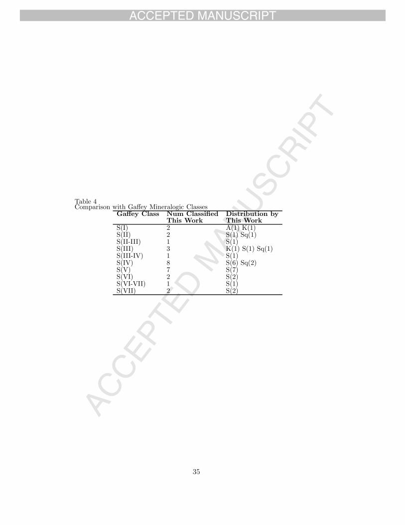
detail revealed only in the near-infrared wavelengths. In Table 4 we list the

classes of featured objects in our system that fall under each of the Gaffey min-

eralogic classes (Gaffey et al., 1993). Taxonomy PCA is sensitive to spectral

features which often, but not always, have mineralogic implications. Thus

a direct mapping from PCA space to mineralogy can only be considered

as a general trend. For example, in Fig. 2, the trend from A-type (inter-

preted as olivine-rich) to V-type (pyroxene-rich) goes from lower left to

upper right. Examining the placement of Gaffey class S(I) (olivine-rich)

through S(VII) (pyroxene-rich) follows this same trend. These objects

generally fall in our S- and Sq-classes. A figure of the Gaffey labels plot-

ted in our principal component space is available in the Supplementary

Material.

A verbal description of each class is given in Table 5, explaining the key spectral fea-

tures and attributes of each particular class and listing at most three objects within

our sample that are considered prototypical of that class. This table also summa-

rizes why the three Bus classes (Ld, Sl, Sk) were not continued in this taxonomy.

A more quantitative summary of the taxonomy is given in the supplementary

material where tables are provided with the mean value and standard

25

ACCEP

TED M

ANUSC

RIPT

ACCEPTED MANUSCRIPT

deviation for the slope and the five principal component for each class,

as well as the mean values and standard deviation for each wavelength

channel for each class. The supplementary material also provides princi-

pal component scores for all 371 objects used to create this taxonomy.

Appendix B shows the flowchart to apply this taxonomy to new data. As in Bus

(1999) it is a binary response decision tree used to locate the position of the object

in multidimensional principal component space, which corresponds to the presence

or absence of features that characterize each class.

[Fig. 15 Key of the 24 Taxonomic Classes]

[Table 2: The evolution of the classes from the Bus (1999) taxonomy to this work]

[Table 3: Comparison with Bus and Tholen Taxonomies]

[Table 4: Comparison with Gaffey Minerologies]

[Table 5: Description of Taxonomic Classes]

6 Conclusion

An extended taxonomy was created using Principal Component Analysis and visible

features to characterize visible and near-infrared wavelength spectra. The system,

based on the Bus visible taxonomy from Bus (1999); Bus and Binzel (2002b), has 24

classes compared to 26 in the Bus system. The changes in classes are summarized

in Table 2. We eliminated three classes: Ld, Sl, and Sk. All the Bus S subclasses

(Sa, Sl, Sk, Sq, Sr) had objects that merged back into the S-class, although many

Sq objects remained Sq and two Sr objects were relabeled Sa. A new intermediate

class, the Sv-class, was created as a link between the S- and V-classes. High-

sloped S, Sq, Sr, Sv, V and Q objects were given a w notation to indicate possible

weathering. Many of the classes that lie left of line α in PC2′ versus PC1′ space

26

ACCEP

TED M

ANUSC

RIPT

ACCEPTED MANUSCRIPT

are either featureless or exhibit only small features at visible wavelengths identified

by Bus (1999); Bus and Binzel (2002b). It is still necessary to use these visible

features to distinguish the classes because there are no other corresponding fea-

tures at near-infrared wavelengths. We have also devised a method to categorize

data when solely the near-infrared wavelength range is available, however, with-

out visible wavelength information, the near-infrared taxonomy supplement cannot

definitively classify many types especially those in the C- and X-complex, as many

of those classes are defined only by visible wavelength features. 371 objects

were given types based on this new taxonomic system which was created using 6 di-

mensions including Slope and PC1′ through PC5′ of Principal Component Analysis.

Within our sample, several classes remain relatively rare: only 6 objects

fall into the A-class; 349 Dembowska and 3628 Boznemcova reside as the

only objects in their respective R- and O-classes. Eight Q-class objects

are all near-Earth asteroids. We note 1904 Massevitch as an outer main-

belt V-type while 15 other V-type objects have inner main-belt orbits

consistent with an association with Vesta.

Acknowledgements

We are grateful to numerous colleagues and students who have participated in or

contributed to the collection or processing of data throughout the course of this

project. These people include, but are not limited to, Mirel Birlan, Thomas Bur-

bine, Jim Elliot, Susan Kern, Alison Klesman, Andrew Rivkin, Paul Schechter,

Shaye Storm, Cristina Thomas, and Pierre Vernazza. Particular thanks for their ad-

vice and insight to Cristina Thomas, Pierre Vernazza, Jessica Sunshine, and Benoit

Carry and to Nick Moscovitz for sharing principal component information of his

data. We especially thank Maureen Bell and Beth Clark for sharing their unpub-

lished spectra to improve class boundaries. Thanks to the anonymous referees for

27

ACCEP

TED M

ANUSC

RIPT

ACCEPTED MANUSCRIPT

their many constructive improvements. Observations reported here were obtained

at the Infrared Telescope Facility, which is operated by the University of Hawaii un-

der Cooperative Agreement NCC 5-538 with the National Aeronautics and Space

Administration, Science Mission Directorate, Planetary Astronomy Program. This

paper includes data gathered with the 6.5 meter Magellan Telescopes located at

Las Campanas Observatory, Chile. Observations in this paper were also obtained

at the Kitt Peak National Observatory, National Optical Astronomy Observatory,

which is operated by the Association of Universities for Research in Astronomy,

Inc. (AURA) under cooperative agreement with the National Science Foundation.

F. E. D. acknowledges funding from the Fulbright Program. This material is based

upon work supported by the National Science Foundation under Grant 0506716

and NASA under Grant NAG5-12355. Any opinions, findings, and conclusions or

recommendations expressed in this material are those of the authors and do not

necessarily reflect the views of the National Science Foundation or NASA. Je donne

mes excuses sinceres pour ne pas avoir reussi a classifier l’asteroıde B612.

References

R. P. Binzel, S. Xu, S. J. Bus, M. F. Skrutskie, M. R. Meyer, P. Knezek, and

E. S. Barker. Discovery of a Main-Belt Asteroid Resembling Ordinary Chondrite

Meteorites. Science, 262:1541–1542, December 1993.

R. P. Binzel, A. W. Harris, S. J. Bus, and T. H. Burbine. Spectral Properties of Near-

Earth Objects: Palomar and IRTF Results for 48 Objects Including Spacecraft

Targets (9969) Braille and (10302) 1989 ML. Icarus, 151:139–149, June 2001.

R. P. Binzel, M. Birlan, S. J. Bus, A. W. Harris, A. S. Rivkin, and S. Fornasier. Spec-

tral observations for near-Earth objects including potential target 4660 Nereus :

Results from Meudon remote observations at the NASA Infrared Telescope Fa-

cility (IRTF). Planetary and Space Science, 52:291–296, March 2004a.

28

ACCEP

TED M

ANUSC

RIPT

ACCEPTED MANUSCRIPT

R. P. Binzel, E. Perozzi, A. S. Rivkin, A. Rossi, A. W. Harris, S. J. Bus, G. B.

Valsecchi, and S. M. Slivan. Dynamical and compositional assessment of near-

Earth object mission targets. Meteoritics and Planetary Science, 39:351–366,

March 2004b.

R. P. Binzel, A. S. Rivkin, J. S. Stuart, A. W. Harris, S. J. Bus, and T. H. Bur-

bine. Observed spectral properties of near-Earth objects: results for population

distribution, source regions, and space weathering processes. Icarus, 170:259–294,

August 2004c.

R. P. Binzel, G. Masi, and S. Foglia. Prediction and Confirmation of V-type As-

teroids Beyond 2.5 AU Based on SDSS Colors. In Bulletin of the American As-

tronomical Society, volume 38 of Bulletin of the American Astronomical Society,

pages 627, September 2006.

R. P. Binzel, G. Masi, S. Foglia, P. Vernazza, T. H. Burbine, C. A. Thomas, F. E.

Demeo, D. Nesvorny, M. Birlan, and M. Fulchignoni. Searching for V-type and

Q-type Main-Belt Asteroids Based on SDSS Colors. In Lunar and Planetary

Institute Conference Abstracts, volume 38 of Lunar and Planetary Inst. Technical

Report, pages 1851, March 2007.

T. H. Burbine. Forging Asteroid-Meteorite Relationships Through Reflectance Spec-

troscopy. PhD thesis, Massachusetts Institute of Technology, 2000.

T. H. Burbine and R. P. Binzel. Small Main-Belt Asteroid Spectroscopic Survey in

the Near-Infrared. Icarus, 159:468–499, October 2002.

S. J. Bus. Compositional structure in the asteroid belt: Results of a spectroscopic

survey. PhD thesis, Massachusetts Institute of Technology, January 1999.

S. J. Bus and R. P. Binzel. Phase II of the Small Main-Belt Asteroid Spectroscopic

Survey, The Observations. Icarus, 158:106–145, July 2002a.

S. J. Bus and R. P. Binzel. Phase II of the Small Main-Belt Asteroid Spectroscopic

Survey, A Feature-Based Taxonomy. Icarus, 158:146–177, July 2002b.

C. R. Chapman, T. V. Johnson, and T. B. McCord. A Review of Spectrophotometric

29

ACCEP

TED M

ANUSC

RIPT

ACCEPTED MANUSCRIPT

Studies of Asteroids. In T. Gehrels, editor, IAU Colloq. 12: Physical Studies of

Minor Planets, pages 51–65, 1971.

B. E. Clark, B. Hapke, C. Pieters, and D. Britt. Asteroid Space Weathering and

Regolith Evolution. Asteroids III, pages 585–599, 2002.

M. Cohen, R. G. Walker, M. J. Barlow, and J. R. Deacon. Spectral irradiance

calibration in the infrared. I - Ground-based and IRAS broadband calibrations.

Astronomical Journal, 104:1650–1657, October 1992.

F. DeMeo and R. P. Binzel. Comets in the near-Earth object population. Icarus,

194:436–449, April 2008.

M. J. Gaffey, T. H. Burbine, J. L. Piatek, K. L. Reed, D. A. Chaky, J. F. Bell, and

R. H. Brown. Mineralogical variations within the S-type asteroid class. Icarus,

106:573–602, December 1993.

E. S. Howell, E. Merenyi, and L. A. Lebofsky. Classification of asteroid spectra

using a neural network. Journal of Geophysical Research, 99:10847–10865, May

1994.

D. A. Jackson. Stopping rules in Principal Component Analysis: A comparison of

heuristical and statistical approaches. Ecology, 74:2202–2214, 1993.

D. Lazzaro, T. Michtchenko, J. M. Carvano, R. P. Binzel, S. J. Bus, T. H. Burbine,

T. Mothe-Diniz, M. Florczak, C. A. Angeli, and A. W. Harris. Discovery of a

Basaltic Asteroid in the Outer Main Belt. Science, 288:2033–2035, June 2000.

S. D. Lord. A new software tool for computing earth’s atmospheric transmission of

near- and far-infrared radiation. NASA Tech. Mem., (103957), 1992.

N. A. Moskovitz, R. Jedicke, E. Gaidos, M. Willman, D. Nesvorny, R. Fevig, and

Z. Ivezic. The Distribution of Basaltic Asteroids in the Main Belt. Icarus, 198:

77–90, November 2008.

J. T. Rayner, D. W. Toomey, P. M. Onaka, A. J. Denault, W. E. Stahlberger, W. E.

Vacca, M. C. Cushing, and S. Wang. Spex: A medium-resolution 0.8-5.5 micron

spectrograph and imager for the nasa infrared telescope facility. Astron. Soc. of

30

ACCEP

TED M

ANUSC

RIPT

ACCEPTED MANUSCRIPT

the Pacific, 115:362–382, 2003.

A. S. Rivkin, R. P. Binzel, and S. J. Bus. Constraining near-Earth object albedos

using near-infrared spectroscopy. Icarus, 175:175–180, May 2005.

D. J. Tholen. Asteroid taxonomy from cluster analysis of photometry. PhD thesis,

University of Arizona, 1984.

D. Tody. Iraf in the nineties. in astronomical data. In Astronomical Data Analysis

Software and Systems II, 1993.

X. H. J. Wood and G. P. Kuiper. Photometric Studies of Asteroids. Astrophysical

Journal, 137:1279–1285, May 1963.

S. Xu. CCD Photometry and Spectroscopy of Small Main-Belt Asteroids. PhD

thesis, Massachusetts Institute of Technology, 1994.

S. Xu, R. P. Binzel, T. H. Burbine, and S. J. Bus. Small main-belt asteroid spec-

troscopic survey: Initial results. Icarus, 115:1–35, May 1995.

B. Zellner, D. J. Tholen, and E. F. Tedesco. The eight-color asteroid survey: Results

for 589 minor planets. Icarus, 61:335–416, February 1985.

31

ACCEP

TED M

ANUSC

RIPT

ACCEPTED MANUSCRIPT

Table 1Variance of Slope and Principal Components

Principal Variance (%) Variance (%)Component (slope excluded) (slope included)

Slope - 88.4PC1’ 63.1 7.3PC2’ 24.3 2.8PC3’ 8.9 1.0PC4’ 2.2 0.3PC5’ 0.6 0.1PC6’ 0.3 0.1PC7’ 0.2 -PC8’ 0.1 -PC9’ 0.1 -

PC10’-PC40’ 0.1 -Total: 100.0 100.0

7 Tables

32

ACCEP

TED M

ANUSC

RIPT

ACCEPTED MANUSCRIPT

Table 2Evolution from the Bus (1999) Taxonomy to This Work

Bus NewA =⇒ AB =⇒ BC =⇒ C

Cb =⇒ CbCg =⇒ Cg

Cgh =⇒ CghCh =⇒ ChD =⇒ D

Ld ↗↘

L =⇒ LK =⇒ KO =⇒ OQ −→ QR =⇒ R

Sq −→ Sr, Srw−→ Sq, Sqw

Sr −→ SaSaSl ↘ S, SwSk ↗S

−→ Sv, SvwT =⇒ TV −→ V, VwX =⇒ X

Xc =⇒ XcXe =⇒ XeXk =⇒ Xk

Total: 26 24Eliminated: Created:

Ld, Sk, Sl Svw notation does not denote a distinct class

The double arrow is used for unchanged classes.

The single arrow is used for classes that are modified.

33

ACCEPTED MANUSCRIPT

AC

CE

PT

ED

MA

NU

SC

RIP

T

Table 3. Comparison with Bus and Tholen TaxonomiesClass Classified Classified Classified Distribution by Distribution by

This Work By Bus By Tholen Bus Class Tholen ClassA 6 6 6 A(5) Sl(1) A(5) S(1)B 4 3 3 B(2) C(1) B(1) F(1) BCF(1)C 12 12 11 C(9) B(2) Cb(1) C(6) CF(1) CU(1) CX(1) G(1) FC(1)Cb 3 3 3 Cb(3) CF(1) M(1) XC:(1)Cg 1 1 1 Cg(1) C(1)Cgh 10 10 7 Cgh(5) Cg(1) Ch(2) C(1) Xc(1) C(4) CU(1) G(1) E(1)Ch 18 18 18 Ch(18) C(10) G(4) CG(2) S(1) X(1)D 16 12 7 D(4) X(3) T(3) Ld(1) L(1) D(4) DU(1) ST(1) X(1)K 16 15 12 K(10) S(1) L(1) Xk(1) Xc(1) Sq(1) S(10) SU(1) T(1)L 22 21 10 L(10) K(5) Ld(4) A(1) S(1) S(7) STGD (1) TSD(1) I(1)O 1 1 0 O(1)Q 8 5 2 Q(3) O(1) Sq(1) Q(1) QU(1)R 1 1 1 R(1) R(1)S 144 122 65 S(88) Sl(10) Sa(8) Sq(7) A(4) Sk(2) Sr(r) L(1) S(60) AS(1) DU(1) QSV(1) SR(1) SU(1)Sa 2 2 0 Sr(2)Sq 29 24 10 Sq(6) Sk(5) S(9) Sa(3) Sr(1) S(9) SQ(1)Sr 22 19 2 Sq(8) S(8) Sa(1) Sr(1)V(1) S(2)Sv 2 0 0T 4 4 4 T(4) T(2) D(1) PCD(1)V 17 11 3 V(9) R(2) V(3)X 8 7 7 X(7) M(4) P(3)Xc 3 3 3 X(2) Xk(1) M(2) X(1)Xe 7 7 6 Xe(7) E(3) M(2) MU(1)Xk 15 14 12 Xk(5) X(5) Xc(2) K(1) C(1) M(3) P(2) X(2) S(1) T(1) C(1) CX(2)Total 371 321 193

34

ACCEP

TED M

ANUSC

RIPT

ACCEPTED MANUSCRIPT

Table 4Comparison with Gaffey Mineralogic Classes

Gaffey Class Num Classified Distribution byThis Work This Work

S(I) 2 A(1) K(1)S(II) 2 S(1) Sq(1)S(II-III) 1 S(1)S(III) 3 K(1) S(1) Sq(1)S(III-IV) 1 S(1)S(IV) 8 S(6) Sq(2)S(V) 7 S(7)S(VI) 2 S(2)S(VI-VII) 1 S(1)S(VII) 2 S(2)

35

ACCEP

TED M

ANUSC

RIPT

ACCEPTED MANUSCRIPT

Table 5Spectral Class DescriptionsClass Description Prototypes

A Deep and extremely broad absorption band with a minimum near 1 μm, may or may nothave shallow 2-μm absorption band; very highly sloped.

246, 289, 863

B Linear, negatively sloping often with a slight round bump around 0.6 μm and/or a slightlyconcave up curvature in the 1- to 2-μm region.

2, 3200

C Linear, neutral visible slope often a slight rough bump around 0.6 μm and low but positiveslope after 1.3. May exhibit slight feature longward of 1 μm.

1, 10, 52

Cb Linear with a small positive slope that begins around 1.1 μm. 191, 210, 785

Cg Small positive slope that begins around 1.3 microns and pronounced UV dropoff. (contentremoved)

175

Cgh Small positive slope that begins around 1 micron and pronounced UV dropoff similar to Cg(content removed) also includes a broad, shallow absorption band centered near 0.7 μmsimilar to Ch.

106, 706, 776

Ch Small positive slope that begins around 1.1 microns and slightly pronounced UV dropoff(content removed) also includes a broad, shallow absorption band centered near 0.7 μm.

19, 48, 49

D Linear with very steep slope, some show slight curvature or gentle kink around 1.5 μm. 1143, 1542, 3248

K Wide absorption band centered just longward of 1 μm, the left maximum and the minimumare sharply pointed and the walls of the absorption are linear with very little curvature.

42, 579, 742

L Steep slope in visible region leveling out abruptly around 0.7 μm. There is often a gentleconcave down curvature in the infrared with a maximum around 1.5 μm. There may or maynot be a 2-micron absorption feature.

236, 402, 606

O Very rounded and deep, bowl shape absorption feature at 1 micron as well as a significantabsorption feature at 2 μm.

3628

Q Distinct 1-μm absorption feature with evidence of another feature near 1.3 μm; a 2-μm featureexists with varying depths between objects.

1862, 3753, 5660

R Deep 1- and 2-μm features; the one-micron feature is much narrower than a Q-type, butslightly broader than a V-type.

349

S Moderate 1- and 2-μm features. The 2-micron feature may vary in depth between objects. 5, 14, 20

Sa Has a deep and extremely broad absorption band at 1 μm; has similar features to A-typesbut is less red.

984, 5261

Sq Has a wide 1-μm absorption band with evidence of a feature near 1.3 μm like the Q-type,except the 1-μm feature is more shallow for the Sq.

3, 11, 43

Sr Has a fairly narrow 1-μm feature similar to but more shallow than an R-type as well as a2-μm feature.

237, 808, 1228

Sv Has a very narrow 1-μm absorption band similar to but more shallow than a V-type as wellas a 2-μm feature.

2965, 4451

T Linear with moderate to high slope and often gently concaving down. 96, 308, 773

V Very strong and very narrow 1-μm absorption and as well as a strong 2-μm absorption feature. 4, 1929, 2851

X Linear with medium to high slope. 22, 87, 153

Xc Low to medium slope and slightly curved and concave downward. 21, 97, 739

Xe Low to medium slope similar to either Xc- or Xk-type, but with an absorption band featureshortward of 0.55 μm.

64, 77, 3103

Xk Slightly curved and concave downward similar to Xc-type but with a faint to feature between0.8 to 1 μm.

56, 110, 337

Ld Diverged to L- and D-classes. 279 (D), 3734 (L)

Sk Diverged to the S- and Sq-classes. 6585 (S), 3 (Sq)

Sl Merged with the S-class. 17 (S), 30 (S)

36

ACCEP

TED M

ANUSC

RIPT

ACCEPTED MANUSCRIPT

8 Figure Captions

Fig. 1. Results for PC1 versus Slope. PC1 is the first principal component from

a data set that did not have the slope removed. It is clear from the plot that PC1

and slope are linearly related and it is thus valid to remove the slope before running

PCA to make PCA more sensitive to other features. Our treatment of slope as a

tabulated and removed parameter follows the method of Bus (1999).

Fig. 2. Results for PC2′ versus PC1′. All objects plotted are labeled with their

taxonomic classification in this system. Notice the “grand divide” between the S-

complex and the C- and X-complexes. Line α separates objects with and without

2-μm absorption bands. The direction orthogonal to line α (increasing PC2′ values)

indicates deeper 2-μm and narrower 1-μm absorption bands. The direction par-

allel to line α (increasing PC1′ values) indicates wider 1-μm absorption

bands. The notation “PC1′”, “PC2′”, etc. denotes that these principal components

are computed after removal of the slope.

Fig. 3. PC2′ versus PC1′ plotted for the S-complex plus A-, Q-, O-, R-,

and V-types. Boundaries chosen for each class are shown and lines are

labeled with greek letters. As described in the text, all boundaries are

perpendicular or parallel to line α.

Fig. 4. PC2′ versus PC1′ plotted for the C- and X-complexes plus D-,

K-, L-, and T-types. This principal component space does not clearly

separate the classes.

Fig. 5. Examples of S-, Sa-, and A-classes. There is a clear progression from S-types

with a shallow one-micron band and low slope to A-types with a deep one-micron

band and high slope. Sa- and A-types show similar 1-μm band absorptions, but

Sa-types are much less red than A-types. The class and the asteroid number

37

ACCEP

TED M

ANUSC

RIPT

ACCEPTED MANUSCRIPT

are labeled next to each spectrum.

Fig. 6. Comparison of prototypes for the V-, O-, Q-, and R-classes. Note

the O-class has a very wide 1-micron band and the V-class has a very

narrow band. The V-types with the deepest 2-micron bands plot farthest

from line α. For this and all subsequent spectral plots: We present relative

reflectances normalized to unity at 0.55 microns; the spectra are offset

vertically for clarity of comparison. The class and asteroid number are

labeled next to each spectrum.

Fig. 7. Comparison of spectra within the S-complex (S, Sq, Sr, Sv) showing

the variation in the one-micron absorption band among these types. Sq-

types have the widest one-micron feature, similar to the Q-class. Sv-types

have the narrowest feature, similar to the V-class.

Fig. 8. Illustration of S and Sw reflectance spectra. The absorption features for

both are very similar. Slope is the most significant distinction between the two,

where the “w” is a notation to denote the slope difference, but does not describe

a distinct class. These two spectra are not offset vertically, showing their

differences relative to their common normalization at 0.55 μm.

Fig. 9. Plot of Slope versus PC1′ for the S-Complex. All objects in classes S, Sq,

Sr and Sv with slopes greater than 0.25 have a “w” notation to denote the high

slope. This “w” notation not describe a distinct class.

Fig. 10. The distribution of objects left of line α in slope versus PC1′ space. Here

we see a clear separation for D- and T-types because of their high slopes. L-types

are distinguished here by their positive PC1′ values. C-complex objects have the

lowest PC′ values while X-complex and K-types reside between the L-types and

C-complex.

38

ACCEP

TED M

ANUSC

RIPT

ACCEPTED MANUSCRIPT

Fig. 11. Prototype examples of D-, L-, K-, T-, and X-class spectra.

Fig. 12. Close examination of principal component distribution for the

C-complex in PC5′ versus PC1′ space. This figure shows that C-types objects plot

to the bottom left, while Xc-, Xe-, and Xk-types plot above the C-class with higher

PC1′ values. Cgh-types have higher PC5′ values than other objects, and are plotted

further right.

Fig. 13. view of the C-complex in PC4′ versus PC1′ space. Here we see the C-types

plotting in the bottom left of the figure and the Ch-types and Cgh-types having

higher PC4′ values plot further to the right.

Fig. 14. Prototype examples for C- and X-complex spectra.

Fig. 15. A “key” showing all 24 taxonomic classes defined over 0.45 -

2.45 μm. The average spectra are plotted with constant horizontal and vertical

scaling and are arranged in a way that approximates the relative position of each

class in the primary spectral component space defined by slope, PC1′, and PC2′

(roughly following Fig. 2). Thus the depth and width of the 2-μm band

generally increases lower left to upper right, and the depth and width

of the 1-μm band increase moving downward and toward the right. For

subtly featured objets slope increases from bottom to top. Due to the spectral

complexity of the C- and X-complexes, the locations of some of these classes do not

strictly follow the pattern. The horizontal lines to which each spectrum is referenced

has a reflectance value of unity. This figure and description follows the style of

Bus and Binzel (2002b, Fig. 15).

39

ACCEP

TED M

ANUSC

RIPT

ACCEPTED MANUSCRIPT

Fig. 1.

Fig. 2.

40

ACCEP

TED M

ANUSC

RIPT

ACCEPTED MANUSCRIPT

Fig. 3.

Fig. 4.

41

ACCEP

TED M

ANUSC

RIPT

ACCEPTED MANUSCRIPT

Fig. 5.

Fig. 6.

42

ACCEP

TED M

ANUSC

RIPT

ACCEPTED MANUSCRIPT

Fig. 7.

Fig. 8.

43

ACCEP

TED M

ANUSC

RIPT

ACCEPTED MANUSCRIPT

Fig. 9.

Fig. 10.

44

ACCEP

TED M

ANUSC

RIPT

ACCEPTED MANUSCRIPT

Fig. 11.

Fig. 12.

45

ACCEP

TED M

ANUSC

RIPT

ACCEPTED MANUSCRIPT

Fig. 13.

Fig. 14.

46

ACCEP

TED M

ANUSC

RIPT

ACCEPTED MANUSCRIPT

AAAAAAAAAAAAAAAAAAAAAAAAAAAAAAAAAAAAAAAAABBBBBBBBBBBBBBBBBBBBBBBBBBBBBBBBBBBBBBBBB

CCCCCCCCCCCCCCCCCCCCCCCCCCCCCCCCCCCCCCCCC

CbCbCbCbCbCbCbCbCbCbCbCbCbCbCbCbCbCbCbCbCbCbCbCbCbCbCbCbCbCbCbCbCbCbCbCbCbCbCbCbCb

CgCgCgCgCgCgCgCgCgCgCgCgCgCgCgCgCgCgCgCgCgCgCgCgCgCgCgCgCgCgCgCgCgCgCgCgCgCgCgCgCgCghCghCghCghCghCghCghCghCghCghCghCghCghCghCghCghCghCghCghCghCghCghCghCghCghCghCghCghCghCghCghCghCghCghCghCghCghCghCghCghCgh

ChChChChChChChChChChChChChChChChChChChChChChChChChChChChChChChChChChChChChChChChCh

DDDDDDDDDDDDDDDDDDDDDDDDDDDDDDDDDDDDDDDDD

KKKKKKKKKKKKKKKKKKKKKKKKKKKKKKKKKKKKKKKKK

LLLLLLLLLLLLLLLLLLLLLLLLLLLLLLLLLLLLLLLLL

OOOOOOOOOOOOOOOOOOOOOOOOOOOOOOOOOOOOOOOOOQQQQQQQQQQQQQQQQQQQQQQQQQQQQQQQQQQQQQQQQQ

RRRRRRRRRRRRRRRRRRRRRRRRRRRRRRRRRRRRRRRRR

SSSSSSSSSSSSSSSSSSSSSSSSSSSSSSSSSSSSSSSSS

SaSaSaSaSaSaSaSaSaSaSaSaSaSaSaSaSaSaSaSaSaSaSaSaSaSaSaSaSaSaSaSaSaSaSaSaSaSaSaSaSa

SqSqSqSqSqSqSqSqSqSqSqSqSqSqSqSqSqSqSqSqSqSqSqSqSqSqSqSqSqSqSqSqSqSqSqSqSqSqSqSqSq

SrSrSrSrSrSrSrSrSrSrSrSrSrSrSrSrSrSrSrSrSrSrSrSrSrSrSrSrSrSrSrSrSrSrSrSrSrSrSrSrSr

SvSvSvSvSvSvSvSvSvSvSvSvSvSvSvSvSvSvSvSvSvSvSvSvSvSvSvSvSvSvSvSvSvSvSvSvSvSvSvSvSvTTTTTTTTTTTTTTTTTTTTTTTTTTTTTTTTTTTTTTTTT

VVVVVVVVVVVVVVVVVVVVVVVVVVVVVVVVVVVVVVVVV

XXXXXXXXXXXXXXXXXXXXXXXXXXXXXXXXXXXXXXXXX

XcXcXcXcXcXcXcXcXcXcXcXcXcXcXcXcXcXcXcXcXcXcXcXcXcXcXcXcXcXcXcXcXcXcXcXcXcXcXcXcXc

XeXeXeXeXeXeXeXeXeXeXeXeXeXeXeXeXeXeXeXeXeXeXeXeXeXeXeXeXeXeXeXeXeXeXeXeXeXeXeXeXeXkXkXkXkXkXkXkXkXkXkXkXkXkXkXkXkXkXkXkXkXkXkXkXkXkXkXkXkXkXkXkXkXkXkXkXkXkXkXkXkXk

Fig. 15.

47

ACCEPTED MANUSCRIPT

AC

CE

PT

ED

MA

NU

SC

RIP

T

Appendix A. Observationsa and Designations

Obj Name Tholen Bus This Work Date Obj Name Tholen Bus This Work Date1 Ceres G C C 19-May-05 52 Europa CF C C 28-Jun-062 Pallas B B B 29-Mar-01 54 Alexandra C C Cgh 27-Oct-023 Juno S Sk Sq 17-Mar-03 55 Pandora M X X 29-Jan-064 Vesta V V V 09-Oct-00 56 Melete P Xk Xk 22-Sep-045 Astraea S S S 20-Feb-04 57 Mnemosyne S S S 01-Jun-027 Iris S S S 20-Feb-04 58 Concordia C Ch Ch 02-Aug-038 Flora S Sw 16-Sep-02 b 61 Danae S S S 08-Oct-0010 Hygiea C C C 19-Feb-04 63 Ausonia S Sa Sw 30-Sep-0311 Parthenope S Sk Sq 13-Nov-05 64 Angelina E Xe Xe 30-Jan-0113 Egeria G Ch Ch 19-May-05 65 Cybele P Xc Xk 30-Sep-0314 Irene S S S 17-May-01 66 Maja C Ch Ch 22-Nov-0515 Eunomia S S K 19-Feb-04 67 Asia S S S 16-Jun-0416 Psyche M X X 09-Oct-00 69 Hesperia M X Xk 11-May-0517 Thetis S Sl S 15-Aug-01 70 Panopaea C Ch Cgh 29-Sep-0218 Melpomene S S S 22-Jun-01 73 Klytia S S 16-Oct-03 b,c

19 Fortuna G Ch Ch 29-Jan-06 76 Freia P X X 05-Sep-0520 Massalia S S S 22-Jun-01 77 Frigga MU Xe Xe 25-Oct-0621 Lutetia M Xk Xc 22-Sep-04 78 Diana C Ch Ch 31-Oct-0522 Kalliope M X X 25-Oct-06 82 Alkmene S Sq S 24-Aug-0124 Themis C B C 08-Oct-05 84 Klio G Ch Ch 02-Aug-0325 Phocaea S S S 30-Jan-01 85 Io FC B C 02-Aug-0326 Proserpina S S S 24-Aug-01 87 Sylvia P X X 04-Sep-0527 Euterpe S S S 22-Sep-04 90 Antiope C C C 05-Sep-0528 Bellona S S S 13-Jan-02 92 Undina X Xc Xk 08-Oct-0029 Amphitrite S S S 29-Jan-01 93 Minerva CU C C 27-Apr-0330 Urania S Sl S 08-Oct-00 96 Aegle T T T 28-Jan-0632 Pomona S S Sw 30-Jan-01 97 Klotho M X Xc 08-Oct-0533 Polyhymnia S Sq S 06-Mar-02 99 Dike C Xk Xk 13-Nov-0534 Circe C Ch Ch 20-Feb-04 101 Helena S S S 22-Dec-0637 Fides S S S 15-Aug-01 103 Hera S S S 14-Aug-0138 Leda C Cgh Cgh 05-Jul-03 105 Artemis C Ch Ch 02-Aug-0339 Laetitia S S Sqw 14-Aug-01 106 Dione G Cgh Cgh 02-Aug-0340 Harmonia S S S 16-Oct-04 108 Hecuba S Sl Sw 06-Mar-0241 Daphne C Ch Ch 15-Sep-04 110 Lydia M X Xk 29-Jan-0142 Isis S L K 21-Jun-01 111 Ate C Ch Ch 22-Sep-0443 Ariadne S Sk Sq 22-Nov-05 114 Kassandra T Xk K 28-Jun-0648 Doris CG Ch Ch 08-Oct-05 115 Thyra S S S 06-Mar-0249 Pales CG Ch Ch 02-Aug-03 119 Althaea S Sl S 21-Jun-0150 Virginia X Ch Ch 05-Jul-03 128 Nemesis C C C 02-Aug-0351 Nemausa CU Ch Cgh 15-Jun-04 130 Elektra G Ch Ch 29-Mar-01

49

ACCEPTED MANUSCRIPT

AC

CE

PT

ED

MA

NU

SC

RIP

T

Observations and Designations (cont.)

Obj Name Tholen Bus This Work Date Obj Name Tholen Bus This Work Date131 Vala SU Xc K 20-Jul-06 289 Nenetta A A A 04-Sep-00132 Aethra M Xe Xe 05-Sep-05 295 Theresia S S Sw 28-Sep-02133 Cyrene SR S S 22-Jun-01 308 Polyxo T T T 18-Apr-05147 Protogeneia C C C 02-Aug-03 321 Phaeo X X D 29-Sep-02150 Nuwa CX Cb C 02-Aug-03 337 Devosa X X Xk 28-Sep-02151 Abundantia S Sl Sw 13-Nov-05 345 Tercidina C Ch Ch 08-Oct-05153 Hilda P X X 10-May-05 346 Hermentaria S S S 31-May-02158 Koronis S S S 16-Mar-03 349 Dembowska R R R 22-Jun-01160 Una CX C Xk 5-Jul-03 352 Gisela S Sl Sw 22-Jun-01170 Maria S S S 22-Jun-01 354 Eleonora S Sl A 15-Apr-02175 Andromache C Cg Cg 13-Nov-05 359 Georgia CX X Xk 30-Jan-01180 Garumna S Sq Sr 28-Sep-02 371 Bohemia QSV S S 14-Aug-01181 Eucharis S Xk Xk 30-Sep-03 378 Holmia S S S 14-Apr-02188 Menippe S S S 15-Apr-02 387 Aquitania S L L 27-Apr-03191 Kolga XC: Cb Cb 12-Apr-05 389 Industria S S S 24-Aug-01192 Nausikaa S Sl Sw 30-Apr-06 402 Chloe S K L 19-Feb-01199 Byblis X D 17-Mar-03 403 Cyane S S S 27-Apr-03201 Penelope M X X 19-Feb-04 433 Eros S S Sw 17-Aug-02205 Martha C Ch Ch 02-Aug-03 434 Hungaria E Xe Xe 23-Aug-01210 Isabella CF Cb Cb 13-Nov-05 444 Gyptis C C C 15-Aug-01214 Aschera E Xc Cgh 24-Oct-04 446 Aeternitas A A A 14-Aug-01216 Kleopatra M Xe Xe 17-Jun-02 453 Tea S S Sw 15-Aug-01221 Eos S K K 08-Oct-00 456 Abnoba S S 17-Jun-02226 Weringia S S 06-Mar-02 460 Scania K L 17-Jun-02233 Asterope T K Xk 29-Sep-02 485 Genua S S 06-Mar-02234 Barbara S Ld L 22-Dec-06 512 Taurinensis S S Sqw 16-Oct-04236 Honoria S L L 01-May-06 513 Centesima S K K 29-Mar-01237 Coelestina S S Sr 15-Apr-02 532 Herculina S S S 21-Jun-01243 Ida S S Sw 17-Mar-03 570 Kythera ST T D 20-Feb-04244 Sita Sa Sw 29-Mar-01 579 Sidonia S K K 20-Feb-01246 Asporina A A A 09-Mar-05 596 Scheila PCD T T 01-Jun-02250 Bettina M Xk Xk 16-Oct-03 599 Luisa S K L 19-Feb-01258 Tyche S S S 24-Aug-01 606 Brangane TSD K L 29-Sep-02264 Libussa S S S 19-May-05 625 Xenia Sa Sw 20-Feb-01266 Aline C Ch Ch 05-Sep-05 631 Philippina S S S 29-Sep-02267 Tirza DU D D 02-Aug-03 653 Berenike S K K 17-Mar-03269 Justitia Ld D 11-May-05 661 Cloelia S K K 16-Mar-03278 Paulina S S 31-May-02 670 Ottegebe S S 29-Sep-02279 Thule D X D 08-Jan-05 673 Edda S S L 21-Jun-01288 Glauke S S S 29-Sep-02 675 Ludmilla S S Sw 15-Apr-02

50

ACCEPTED MANUSCRIPT

AC

CE

PT

ED

MA

NU

SC

RIP

T

Observations and Designations (cont.)

Obj Name Tholen Bus This Work Date Obj Name Tholen Bus This Work Date679 Pax I K L 19-Feb-01 1204 Renzia S Sw 10-Mar-05688 Melanie C C 28-Sep-02 1228 Scabiosa S Sr 16-Mar-03699 Hela S Sq S 08-Jan-05 1300 Marcelle Cg Cgh 25-Oct-06706 Hirundo Cgh Cgh 30-Jan-06 1329 Eliane S S Sqw 17-Aug-02716 Berkeley S S S 24-Aug-01 1332 Marconia Ld L 10-Jun-05719 Albert S 23-Aug-01 d 1350 Rosselia S Sa S 21-Jun-01720 Bohlinia S Sq Sq 09-Oct-00 1374 Isora Sq Sq 20-Feb-04729 Watsonia STGD L L 14-Aug-01 1433 Geramtina S S 17-Aug-02739 Mandeville X X Xc 28-Sep-02 1459 Magnya Vw 20-Feb-01 b

742 Edisona S K K 16-Mar-03 1471 Tornio T D 08-Oct-05773 Irmintraud D T T 22-Sep-04 1494 Savo Sa Sqw 25-Oct-06776 Berbericia C Cgh Cgh 12-Apr-05 1508 Kemi BCF C B 19-Feb-04782 Montefiore S Sl Sw 22-Jun-01 1542 Schalen D D 18-Apr-05785 Zwetana M Cb Cb 19-May-05 1565 Lemaitre Sq S 03-Mar-05789 Lena X Xk 17-Aug-02 1620 Geographos S S S 29-Jan-01793 Arizona DU: S S 28-Sep-02 1640 Nemo S S 08-Mar-05808 Merxia Sq Sr 14-Aug-01 1642 Hill S S 15-Aug-01824 Anastasia S L L 14-Aug-01 1658 Innes AS Sw 30-Jan-01 c

832 Karin S 05-Jul-03 e 1659 Punkaharju S S 15-Mar-02847 Agnia S S S 19-Feb-01 1660 Wood S S 08-Mar-05863 Benkoela A A A 14-Jan-02 1662 Hoffmann Sr Sr 17-Mar-03908 Buda L D 20-Jul-06 1667 Pels Sa Sw 28-Oct-02913 Otila Sa Sw 15-Aug-01 1685 Toro S S Sq 08-May-02 h

925 Alphonsina S S S 28-Sep-02 1751 Herget S S 22-Jun-01929 Algunde S S 21-Jun-01 1807 Slovakia S Sqw 15-Sep-04944 Hidalgo D D 22-Sep-04 e 1839 Ragazza S S 29-Mar-01984 Gretia Sr Sa 29-Sep-02 1848 Delvaux S S 15-Aug-01985 Rosina S S 11-May-05 1858 Lobachevskij L S 14-Apr-021011 Laodamia S Sr Sw 12-Jan-02 1862 Apollo Q Q Q 13-Nov-051020 Arcadia S Sr 17-Mar-03 1864 Daedalus SQ Sr Sq 29-Mar-011036 Ganymed S S S 09-Mar-05 1866 Sisyphus S Sw 21-Nov-061065 Amundsenia S S 08-Mar-05 1903 Adzhimushkaj K K 17-Mar-031094 Siberia Xk Xk 16-Mar-03 1904 Massevitch R V 04-Sep-001126 Otero A Sw 20-Feb-01 1916 Boreas S Sw 14-Aug-01 d

1131 Porzia S S 11-May-05 1929 Kollaa V V 19-Feb-011139 Atami S S Sw 05-Sep-05 1943 Anteros S Sw 12-Jan-02 g,h

1143 Odysseus D D 10-Jun-05 b 1980 Tezcatlipoca SU Sl Sw 25-Oct-061147 Stavropolis S Sw 15-Aug-01 2035 Stearns E Xe Xe 28-Oct-021148 Rarahu S K K 29-Mar-01 2042 Sitarski Sq Sr 23-Aug-011198 Atlantis Sw 28-Oct-02 b 2045 Peking V V 14-Jan-02

51

ACCEPTED MANUSCRIPT

AC

CE

PT

ED

MA

NU

SC

RIP

T

Observations and Designations (cont.)

Obj Name Tholen Bus This Work Date Obj Name Tholen Bus This Work Date2063 Bacchus Sq Sq 19-May-05 3248 Farinella D D 18-Apr-052064 Thomsen S Sqw 29-Jun-06 3255 Tholen S S 16-Sep-022074 Shoemaker Sw 30-Sep-03 b 3317 Paris T D 01-May-062085 Henan L L 14-Apr-02 3363 Bowen Sq Sr 15-Apr-022099 Opik S Ch Ch 08-Oct-05 3395 Jitka Sr S 19-Feb-012107 Ilmari S Sw 29-Jan-06 3402 Wisdom S 30-Sep-03 e

2157 Ashbrook S S 16-Mar-03 3430 Bradfield Sq S 17-Jun-022246 Bowell D D D 17-Apr-05 3491 Fridolin Sq S 17-Jun-022335 James S 30-Oct-05 3511 Tsvetaeva S Srw 15-Apr-022353 Alva S S 31-May-02 3628 Boznemcova O O 30-Apr-062354 Lavrov L L 17-Mar-03 3635 Kreutz S Srw 12-Nov-052378 Pannekoek Cgh Cgh 11-May-05 3701 Purkyne S S 14-Aug-012386 Nikonov S S 17-Jun-02 3734 Waland Ld L 24-Aug-012396 Kochi Sa S 15-Aug-01 3753 Cruithne Q Q 08-Oct-052401 Aehlita S S 17-Aug-02 3788 Steyaert S S 17-Mar-032442 Corbett V 15-Sep-02 c 3844 Lujiaxi L L 27-Apr-032448 Sholokhov L L 16-Mar-03 3858 Dorchester Sa Srw 20-Feb-042501 Lohja A A A 12-Jan-02 3873 Roddy S Sw 28-Oct-022504 Gaviola Sq Sr 27-Apr-03 3903 Kliment Ohridski Sq S 16-Sep-022521 Heidi S S 13-Jan-02 3908 Nyx V V 15-Sep-042566 Kirghizia V V 16-Sep-02 3910 Liszt S S 17-Aug-022579 Spartacus V V 10-Oct-00 3920 Aubignan Sa Sqw 16-Sep-022715 Mielikki A Sw 15-Aug-01 3949 Mach Sq Sq 24-Aug-012732 Witt A L 15-Aug-01 4038 Kristina Vw 28-Oct-02 d

2851 Harbin V V 24-Aug-01 4055 Magellan V V 11-Apr-05 d

2873 Binzel Sq Sq 13-Jan-02 4179 Toutatis Sk Sq 15-Sep-042875 Lagerkvist S S 16-Mar-02 4188 Kitezh V V 14-Aug-012911 Miahelena S Sw 17-Mar-03 4197 1982 TA Sq Sq 30-Sep-032912 Lapalma V V 20-Feb-01 4352 Kyoto S S 17-Jun-022957 Tatsuo K K 16-Mar-03 4407 Taihaku Sa Sqw 24-Aug-012965 Surikov Sv 10-May-05 b 4417 Lecar S Sw 24-Aug-012977 Chivilikhin S S 28-Sep-02 4451 Grieve Svw 14-Jan-02 d

3028 Zangguoxi K K 16-Sep-02 4558 Janesick S Sr 15-Jun-043102 Krok S Sqw 09-Oct-00 d 4570 Runcorn Sa Sw 21-Jun-013103 Eger Xe Xe 21-Jun-01 i 4688 1980 WF QU Q 29-Jan-01 d

3122 Florence S Sqw 26-Jan-04 4713 Steel A Sw 14-Apr-023155 Lee V V 22-Jun-01 4737 Kiladze L L 17-Jun-023198 Wallonia S Sqw 10-May-05 4995 Griffin S S 28-Oct-023199 Nefertiti S Sq K 03-Mar-05 5013 Suzhousanzhong Sl Sw 14-Jan-023200 Phaethon F B B 10-Dec-04 5111 Jacliff R V 05-Sep-05

52

ACCEPTED MANUSCRIPT

AC

CE

PT

ED

MA

NU

SC

RIP

T

Observations and Designations (cont.)

Obj Name Tholen Bus This Work Date Obj Name Tholen Bus This Work Date5143 Heracles O Q 25-Oct-06 19356 1997 GH3 S Sq 30-Jan-015230 Asahina S S 5-Sep-05 20786 2000 RG62 Sq 1-Sep-03 d

5261 Eureka Sr Sa 19-May-05 20790 2000 SE45 S 29-Jan-01 d

5379 Abehiroshi V Sr 3-Jun-06 22771 1999 CU3 S 16-Oct-03 d

5401 Minamioda S Sw 16-Mar-03 24475 2000 VN2 Sw 29-Mar-01 d

5407 1992 AX Sk S 13-Jan-02 25330 1999 KV4 Xk 27-Oct-02 d

5587 1990 SB Sq Sr 28-Mar-01 35107 1991 VH Sk Sq 27-Dec-025604 1992 FE V 29-Mar-01 f 36284 2000 DM8 K 16-Mar-02 d

5641 McCleese A Sw 12-Apr-05 53435 1999 VM40 Srw 25-Oct-06 g

5660 1974 MA Q Q 22-Aug-93 54690 2001 EB S 28-Mar-01 d

5685 Sanenobufukui S S 29-Mar-01 66146 1998 TU3 Q 1-Sep-03 e

5817 Robertfrazer S Sr 22-Sep-04 86450 2000 CK33 L 29-Jan-01 d

5840 Raybrown Ld L 24-Aug-01 86819 2000 GK137 Sq 9-Oct-00 d

6047 1991 TB1 S S 8-Oct-05 89355 2001 VS78 Sr 16-Mar-026239 Minos Sqw 26-Jan-04 e 98943 2001 CC21 Sw 24-Oct-04 f

6386 Keithnoll S S 3-Mar-05 99907 1989 VA Sq Sr 27-Oct-026411 Tamaga B 20-Feb-04 e 137062 1998 WM Sq Sr 27-Oct-026455 1992 HE S Srw 28-Oct-02 138258 2000 GD2 Sq 16-Oct-03 d

6585 O’Keefe Sk S 25-Oct-06 162058 1997 AE12 Q 15-Mar-027341 1991 VK Sq Q 16-Mar-02 162781 2000 XL44 S 29-Jan-01 d

7763 Crabeels L L 1-Jun-02 2000PG3 D 4-Sep-00 d

8334 1984 CF S S 17-Mar-03 2001TX16 X 15-Mar-02 d

8444 Popovich S 30-Sep-03 e 2001XN254 S 14-Apr-02 d

17274 2000 LC16 D 10-Oct-00 d 2002AA S 13-Jan-02 d

18736 1998 NU Sw 30-Jan-01 d 2002AV S 13-Jan-02 d

19127 Olegefremov Srw 30-Sep-03 e

a All visible data are from Bus (1999), Bus and Binzel (2002a) and Bus and Binzel (2002b) unless marked by a footnote. b Visible data: Xu (1994); Xu et al. (1995). c Visible

data: (2000); Burbine and Binzel (2002). d Binzel et al. (2004c) e Visible data: This Work. 832, 03-Mar-05; 944, 14-June-01; 3402, 01-Sep-03; 6239 29-Dec-03; 6411, 29-Dec-03;

8444, 28-Dec-03; 19127 28-Dec-03; 66146, 3-Sep-03. All these observations were taken on telescope KPNO 4m except 944 on Magellan 6.5m. f Visible data: Binzel et al. (2004b).

g Visible data: Binzel et al. (2001). h Near-IR data: Binzel et al. (2004a). i Near-IR data: Rivkin et al. (2005).

53

ACCEP

TED M

ANUSC

RIPT

ACCEPTED MANUSCRIPT

VIS-IR Step 1

Does it satisfy all:PC1′ < -0.30

no−→ VIS-IR Step 2PC3′ ≥ 0.20Slope ≥ 0.40⏐

⏐�yes

Does it satisfy: yes−→ A0.55 ≤ Slope < 1.5⏐

⏐�no

Does it satisfy: yes−→ Sa0.40 ≤ Slope < 0.55

⏐⏐�no

Indeterminate

Appendix B. Visible - IR Flowchart

54

ACCEP

TED M

ANUSC

RIPT

ACCEPTED MANUSCRIPT

VIS-IR Step 2

Does it lie below yes−→ VIS-IR Step 3line α?⏐⏐�no

Does it line on yes−→ V and if Slope ≥ 0.25−−−−−−−−−−−−−−→Add w notation

or above line δ? Vw⏐⏐�no

Does satisfy both:yes−→ OLies on or below line η.

Lies on or above θand below δ⏐

⏐�no

Does satisfy both: yes−→ Qand if Slope ≥ 0.25−−−−−−−−−−−−−−→

Lies on or below line η. Add w notationLies on or above α Qw

and below θ.⏐⏐�no

Does satisfy both: yes−→ RLies on above line η.Lies on or above γ

and below δ⏐⏐�no

VIS-IR S-Complex

55

ACCEP

TED M

ANUSC

RIPT

ACCEPTED MANUSCRIPT

VIS-IR Step 3

Does it satisfy both:yes−→ D0.38 ≤ Slope < 1.5 A: Prominent 1-μm feature.

−0.44 < PC1′ < 0.4⏐⏐�no

Does it satisfy all:yes−→ T0.25 < Slope < 0.38

−0.28 < PC2′ < −0.20−0.20 < PC3′ < −0.12⏐

⏐�no

Does it satisfy both:0.07 < PC1′ < 1.00 yes−→ L, Xe Xe: Shows feature at 0.49μm.

−0.5 < PC2′ < −0.15⏐⏐�no

Does it satisfy all:−0.075 < PC3′ < 0.14 yes−→ K, Xe Xe: Shows feature at 0.49μm.

−0.20 ≤ PC2′ < −0.10−0.80 < PC1′ < −0.10

⏐⏐�no

VIS-IR C- and X-Complexes

56

ACCEP

TED M

ANUSC

RIPT

ACCEPTED MANUSCRIPT

VIS-IR S-Complex

Does it satisfy both: yes−→ Sand if Slope ≥ 0.25−−−−−−−−−−−−−−→

Add w notationLies below β and above ζ Sw⏐

⏐�no

Does it satisfy all:yes−→ Sq and if Slope ≥ 0.25−−−−−−−−−−−−−−→

Add w notationLies on or above α and below β SqwLies above η and on or below ζ⏐

⏐�no

Does it satisfy all:yes−→ Sr and if Slope ≥ 0.25−−−−−−−−−−−−−−→

Add w notationLies on or above β and below γ SrwLies above η and on or below ε⏐

⏐�no

Does it satisfy all:yes−→ Sv and if Slope ≥ 0.25−−−−−−−−−−−−−−→

Add w notationLies on or above β Svw

Lies above ε and below γ⏐⏐�no

Indeterminate

57

ACCEP

TED M

ANUSC

RIPT

ACCEPTED MANUSCRIPT

VIS-IR C- and X-complexes

Does it satisfy all:yes−→ B-0.2 < Slope < 0

-1.2 < PC1′ < 0PC4′ < 0⏐

⏐�no

X: FeaturelessDoes it satisfy:

yes−→ X, Xk, Xe, C

Xk: Shows feature between 0.8 - 1 μm.0.2 < Slope < 0.38 Xe: Shows feature at 0.49 μm.

C: Shows feature between 1 - 1.3 μm.⏐⏐�no

Does it satisfy all:

yes−→ Cgh0.01 < PC4′ < 0.14-0.75 < PC1′ < -0.27

Reflectance at0.45 μm < 0.92.⏐

⏐�no

Does it satisfy both:yes−→ Ch, Xk0.01 < PC4′ < 0.14 Ch: Shows Shows feature at 0.7 μm.

-0.75 < PC1′ < -0.27 Xk: Shows feature between 0.8 - 1 μm.⏐⏐�no

Does it satisfy both:yes−→ Cb-0.04 < PC4′ < 0.02

-0.07 < PC5′ < -0.04⏐⏐�no

Does it satisfy both:yes−→ C, Ch, Xk

C: Shows feature between 1 - 1.3 μm.-0.85 < PC1′ < -0.45 Ch: Shows feature at 0.7 μm.-0.06 < PC5′ < 0.02 Xk: Shows feature between 0.8 - 1 μm.⏐

⏐�no

Does it satisfy both:yes−→ Cgh, Cg0.02 ≤ PC5′ < 0.1 Cgh: Shows feature at 0.7 μm.

-0.60 < PC1′ < -0.16⏐⏐�no

Does it satisfy both:yes−→ Xk, Xc, Xe,C

Xk: Shows feature between 0.8 - 1 μm.-0.45 ≤ PC1′ < 0.1 Xc: Featureless.-0.06 < PC5′ < 0.05 Xe: Shows feature at 0.49 μm.

C: Shows feature between 1 - 1.3 μm.⏐⏐�no

Does it satisfy both:yes−→ Xe, L-0.1 ≤ PC1′ < 0.3 Xe: Shows feature at 0.49 μm.

-0.5 < PC2′ < -0.2⏐⏐�no

Indeterminate

58

ACCEP

TED M

ANUSC

RIPT

ACCEPTED MANUSCRIPT

VIS-IR Checks 1 for Cg, Cgh, Ch, Xc, Xe, Xk VIS-IR EquationsCg Strong UV absorption feature before 0.55 μm PC1′ = −3PC2′ − 0.28 Line αCh Moderately shallow absorption feature around 0.7 μm PC1′ = −3PC2′ + 0.35 Line βCgh Strong UV absorption feature like Cg and 0.7-μm PC1′ = −3PC2′ + 1.00 Line γ

feature like Ch (Reflectance at 0.45 μm < 0.92) PC1′ = −3PC2′ + 1.50 Line δXc Red and featureless with slight concave down curvature PC1′ = 1

3PC2′ + 0.50 Line ε

Xe Concave-up absorption feature before 0.55 μm PC1′ = 13PC2′ − 0.10 Line ζ

Xk Red shortward of 0.75 μm and generally flat PC1′ = 13PC2′ − 0.50 Line η

longward of 0.75 μm PC1′ = −3PC2′ + 0.70 Line θ

1 These spectral features are originally defined in Bus (1999) and Table 2 of Bus and Binzel (2002b).

59

ACCEP

TED M

ANUSC

RIPT

ACCEPTED MANUSCRIPT

Appendix C. IR Flowchart

IR Step 1: End Members

Does it satisfy: no−→ VPCir1′ ≤ 0.5⏐

⏐�no

Does it satisfy all:yes−→ Sv, Sr0.29 ≤ PCir1′ < 0.5

PCir5′ ≤ 0.05⏐⏐�no

Does it satisfy all:yes−→ OPCir2′ ≤ -0.5

PCir4′ ≥ 0.15-0.40 < PCir1′ ≤ 0⏐

⏐�no

Does it satisfy all:yes−→ R0.25 ≤ PCir2′ < 0.5

PCir5′ ≥ 0.06PCir3′ ≥ 0.05⏐

⏐�no

Does it satisfy all:yes−→ DBelow line 1

PCir3′ ≤ -0.02Slopeir ≥ 0.24⏐

⏐�no

Does it satisfy all:

yes−→ A

PCir1′ ≤ -0.4PCir2′ ≤ -0.2PCir4′ ≥ -0.07Slopeir ≥ 0.5PCir3′ ≥ 0⏐

⏐�no

Does it satisfy all: yes−→ SaPCir1′ ≤ -0.4

⏐⏐�no

Step 2

60

ACCEP

TED M

ANUSC

RIPT

ACCEPTED MANUSCRIPT

IR Step 2: S-complex

Does it lie on or yes−→ S, Sr, Sqabove line 1 and 2?⏐⏐�no

Does it lie on oryes−→ S, Sq, Q, L, Kabove line 1 and

between line 2 and 3?⏐⏐�no

Does it line on or aboveyes−→ K, L, Sqline 1 and on or

between line 3 and 4?⏐⏐�no

IR Step 3

IR Step 3: C- and X-complexes

Does it satisfy:yes−→ X-, C-complexes, L, K, TBelow line 1 and on or

between 3 and 4?⏐⏐�no

Does it satisfy: yes−→ X-, C-complexesBelow line 1 andbetween 2 and 3?

⏐⏐�no

Does it satisfy: yes−→ C, B, L, Cb, XBelow line 1 and 4?⏐⏐�no

Indeterminate

IR Equations

PCir3′ =PCir2′ - 0.08 Line 1PCir1′ =PCir2′ + 0.15 Line 2PCir1′ =PCir2′ - 0.10 Line 3PCir1′ =PCir2′ - 0.40 Line 4

61

ACCEP

TED M

ANUSC

RIPT

ACCEPTED MANUSCRIPT

Appendix DReflectance Spectra for 371 Asteroids Defining this Taxonomy

62

ACCEP

TED M

ANUSC

RIPT

ACCEPTED MANUSCRIPT

Reflectance Spectra for 371 Asteroids (cont.)

63

ACCEP

TED M

ANUSC

RIPT

ACCEPTED MANUSCRIPT

Reflectance Spectra for 371 Asteroids (cont.)

64

ACCEP

TED M

ANUSC

RIPT

ACCEPTED MANUSCRIPT

Reflectance Spectra for 371 Asteroids (cont.)

65