An Extended Objective Evaluation of the 29-km Eta Model ... · Eta model attributes ... The AMU's...

NASA Contractor Report CR- 1998-207910

An Extended Objective Evaluation of the 29-km Eta Model

For Weather Support to the United States Space Program

Prepared By:

Applied Meteorology Unit

Prepared for:

Kennedy Space CenterUnder Contract NAS 10-96018

NASANational Aeronautics and

Space Administration

Office of Management

Scientific and Technical

Information Program

1998

https://ntrs.nasa.gov/search.jsp?R=19980210007 2018-08-04T22:19:37+00:00Z

AttributesandAcknowledgments

NASA/KSC POC:

Dr. Francis J. MerceretAA-C-1

Applied Meteorology Unit (AMU)

Paul Nutter

John Manobianeo

ii

Table of Contents

List of Figures ................................................................................................................................................. vi

List of Tables ............................................................................................................................................... viii

Executive Summary ........................................................................................................................................ ix

1.0 Introduction .............................................................................................................................................. 1

1.1 Motivation for Objective Point Forecast Verification ....................................................................... 1

1.2 Precedent and Progress ..................................................................................................................... I

1.3 Applied Meteorology Unit Tasking ................................................................................................... 1

1.4 Report Objectives and Organization ................................................................................................. 2

2.0 Eta Model Overview ................................................................................................................................. 3

3.0 Data and Analysis Method ....................................................................................................................... 3

3. I Data Collection Periods ..................................................................................................................... 3

3.2 Data Collection Methods ................................................................................................................... 3

3.3 Statistical Analysis Methods ............................................................................................................. 4

4.0 Surface Forecast Accuracy ....................................................................................................................... 4

4.1 Overall Summary and Interpretation ................................................................................................. 4

4.2 1996 Surface Forecast Accuracy ....................................................................................................... 7

4.2.1 1996 Warm Season ............................................................................................................. 7

4.2.1.1 Mean Sea-Level Pressure ............................................................................................. 7

4.2.1.2 2-m Tempemtttre .......................................................................................................... 7

4.2.1.3 2-m Dew Point Temperature ........................................................................................ 7

4.2.1.4 10-m Wind Speed ........................................................................................................ 9

4.2.1.5 10-m Wind Direction ................................................................................................... 9

4.2.2 1996 Cool Season ............................................................................................................... 9

4.2.2.1

4.2.2.2

4.2.2.3

4.2.2.4

Mean Sea-Level Pressure ............................................................................................. 9

2-m Temperature .......................................................................................................... 9

2-m Dew Point Temperature ........................................................................................ 9

10-m Wind Speed ...................................................................................................... 11

iii

4.2.2.5 10-m Wind Direction ................................................................................................. 11

4.3 Changes in Surface Forecast Accuracy During 1997 ...................................................................... 11

4.3.1 1997 Warm Season ........................................................................................................... 12

4.3.1.1 Mean Sea-Level Pressure ........................................................................................... 12

4.3.1.2 2-m Temperature ........................................................................................................ 12

4.3.1.3 2-m Dew Point Temperature ...................................................................................... 12

4.3.1.4 10-reWind Speed ...................................................................................................... 15

4.3.1.5 10-m Wind Direction ................................................................................................. 15

4.3.1.6 Summary of 1997 Warm Season Changes ................................................................. 15

4.3.2 1997 Cool Season ............................................................................................................. 16

4.3.2.1 Mean Sea-Level Pressure ........................................................................................... 16

4.3.2.2 2-m Temperature ........................................................................................................ 16

4.3.2.3 2-m DewPoint Temperature ...................................................................................... 16

4.3.2.4 10-m Wind Speed ...................................................................................................... 16

4.3.2.5 10-m Wind Direction ................................................................................................. 19

4.3.2.6 Summary of 1997 Cool Season Changes ................................................................... 19

4.4 10-m Wind Persistence .................................................................................................................... 19

5.0 Upper Air Forecast Accuracy ................................................................................................................. 20

5.1 Summary of Upper-Air Forecast Accuracy ..................................................................................... 20

5.2 Detailed Results ............................................................................................................................... 21

5.2.1 Temperature ...................................................................................................................... 21

5.2.2 Mixing Ratio ..................................................................................................................... 22

5.2.3 Wind Speed ....................................................................................................................... 22

5.2.4 Wind Direction .................................................................................................................. 26

5.2.5 Geopotential Height .......................................................................................................... 26

5.3 Forecast Error Growth ..................................................................................................................... 29

6.0 Convective Indices ................................................................................................................................. 31

6.1 Summary of Convective Index Error Characteristics ...................................................................... 31

iv

6.2 ConvectiveIndexErrorCharacteristics...........................................................................................32

6.2.1 PrecipitableWater.............................................................................................................32

6.2.2 LiftedIndex.......................................................................................................................32

6.2.3 K-Index.............................................................................................................................36

6.2.4 LiftedCondensationLevel................................................................................................36

6.2.5 ConvectiveAvailablePotentialEnergy.............................................................................36

6.2.6 ConvectiveInhibition........................................................................................................40

6.2.7 Helicity..............................................................................................................................40

6.2.8 MicroburstDayPotentialIndex........................................................................................40

7.0 850to500-robLayer-Averages....................................................................................._........................44

8.0WindRegimeStratification....................................................................................................................44

9.0SummaryofSubjectiveForecastValue..................................................................................................45

10.0SummaryandLessonsLearned..............................................................................................................46

10.1SurfaceResults...............................................................................................................................46

10.2Upper-airResults............................................................................................................................46

10.3ConvectiveIndexResults...............................................................................................................47

10.4LayerAverages and Wind Regime Stratification ........................................................................... 47

10.5 Lessons and Recommendations ...................................................................................................... 47

11.0References .............................................................................................................................................. 48

Appendix A ................................................................................................................................................... 51

Appendix B .................................................................................................................................................... 52

Appendix C .................................................................................................................................................... 54

Appendix D ................................................................................................................................................... 58

Appendix E .................................................................................................................................................... 59

V

Figure 4.1.

Figure 4.2.

Figure 4.3.

Figure 4.4.

Figure 4.5.

Figure 4.6.

Figure 5.1.

Figure 5.2.

Figure 5.3.

Figure 5.4.

Figure 5.5.

Figure 5.6.

Figure 6.1.

Figure 6.2.

Figure 6.3.

Figure 6.4.

Figure 6.5.

List of Figures

Bias (forecast - observed), RMS error, and error standard deviation for surface parameterforecasts from the 0300 UTC Meso-Eta cycle during the 1996 warm season ................................... 8

Bias (forecast - observed), RMS error, and error standard deviation for surface parameterforecasts from the 0300 UTC Meso-Eta cycle during the 1996 cool season ........................ . .......... 10

1997 warm season bias (forecast - observed), annual difference of absolute bias (AB97 -AB96), and standardized Z statistics for the 0300 UTC Meso-Eta cycle ........................................ 13

Comparison of annual changes (1997 - 1996) in mean forecasts and observations duringthe warm season .............................................................................................................................. 14

1997 cool season bias (forecast - observed), annual difference of absolute bias (AB97 -

AB96), and standardized Z statistics for the 0300 UTC Meso-Eta cycle ........................................ 17

Comparison of annual changes (1997 - 1996) in mean forecasts and observations duringthe cool season ........................................................................................................ _....................... 18

Bias (forecast - observed), RMS error, and error standard deviation (°C) of temperatureforecasts plotted as a function of pressure level .............................................................................. 23

Bias (forecast - observed), RMS error, and error standard deviation (g kg-1) of mixingratio forecasts plotted as a function of pressure level ...................................................................... 24

Bias (forecast - observed), RMS error, and error standard deviation (m sq) of wind speedforecasts plotted as a function of pressure level .............................................................................. 25

Bias (forecast - observed), RMS error, and error standard deviation (*) of wind directionforecasts plotted as a function of pressure level .............................................................................. 27

Bias (forecast - observed), RMS error, and error standard deviation (m) of geopotentialheight forecasts plotted as a function of pressure level ................................................................... 28

Paired Z statistic plotted as a function of pressure level .................................................................. 30

Quartile diagram showing the conditional distribution of observed PWAT (ram)associated with given forecast values and a histogram of the marginal distribution offorecasts ........................................................................................................................................... 34

Quartile diagram showing the conditional distribution of observed lifted index (°C)associated with given forecast values and a histogram of the marginal distribution offorecasts ........................................................................................................................................... 35

Quartile diagram showing the conditional distribution of observed K-index (°C)

associated with given forecast values and a histogram of the marginal distribution offorecasts ........................................................................................................................................... 37

Quartile diagram showing the conditional distribution of observed LCL (nab) associatedwith given forecast values and a histogram of the marginal distribution of forecasts ...................... 38

Quartile diagram showing the conditional distribution of observed CAPE (J kg "_)associated with given forecast values and a histogram of the marginal distribution offorecasts ........................................................................................................................................... 39

vi

Figure6.6.

Figure6.7.

Figure6.8.

QuartilediagramshowingtheconditionaldistributionofobservedCIN(J kg "_) associated

with given forecast values and a histogram of the marginal distribution of forecasts ...................... 41

Quartile diagram showing the conditional distribution of observed helicity (m 2 s"2)

associated with given forecast values and a histogram of the marginal distribution offorecasts .......................................................................................................................................... 42

Quartile diagram showing the conditional distribution of observed MDPI associated withgiven forecast values and a histogram of the marginal distribution of forecasts ............................. 43

vii

Table 1.1.

Table 3. I.

Table 4.1.

Table 4.2.

Table 4.3.

Table 5.1.

Table 5.2.

Table 6.1.

Table 6.2.

Table 6.3.

Table 7.1.

Table A. 1.

Table C. 1.

Table C.2.

Table C.3.

Table C.4.

Table C.5.

Table C.6

List of Tables

Meso-Eta verification parameters ...................................................................................................... 2

Definition of seasonal verification periods and notable Eta model updates ...................................... 3

Summary of Meso-Eta forecast biases (forecast - observed), RMS errors, and errorstandard deviations for surface parameters at XMR. ......................................................................... 5

Summary of Meso-Eta forecast biases (forecast - observed), RMS errors, and errorstandard deviations for surface parameters at TBW .......................................................................... 6

Summary of Meso-Eta forecast biases (forecast - observed), RMS errors, and errorstandard deviations for surface parameters at EDW .......................................................................... 6

Summary of Meso-Eta upper-air forecast error characteristics at XMR and TBW ......................... 20

Summary of Meso-Eta upper-air forecast error characteristics at EDW .......................................... 21

Summary of Meso-Eta point forecast error characteristics for convective indices at XMRduring the warm season (May-Aug) ................................................................................................ 32

Bias, RMS error and error standard deviation for warm season (May - August) convectiveparameters at XMR and TBW ......................................................................................................... 33

Bias, RMS error and error standard deviation for cool season (October - January)

convective parameters at XMR and TBW ....................................................................................... 33

Warm and cool season bias, RMS error, and error standard deviation for 1000- to 850-rob

thickness and 850- to 500-rob layer-averaged relative humidity, wind speed, and winddirection ........................................................................................................................................... 44

Eta model attributes from Black (1994), Janjic (1994), and Rogers et al. (1996) ........................... 51

Warm season biases for wind variables at XMR and EDW as a function of geopotentialheight ............................................................................................................................................... 55

Cool season biases for wind variables at XMR and EDW as a function of geopotentialheight ............................................................................................................................................... 55

Warm season RMS errors for wind variables at XMR and EDW as a function of

geopotential height .......................................................................................................................... 56

Cool season RMS errors for wind variables at XMR and EDW a function of geopotentialheight ............................................................................................................................................... 56

Warm season error standard deviations for wind variables at XMR and EDW as a

function of geopotential height ........................................................................................................ 57

Cool season error standard deviations for wind variables at EDW as a function of

geopotential height .......................................................................................................................... 57

viii

Executive Summary

This report describes the Applied Meteorology Unit's (AMU) objective verification of the National Centersfor Environmental Prediction ('NCEP) 29-kin Eta (Meso-Eta) numerical weather prediction model. Theverification was designed to identify the model's error characteristics for surface and upper-air point forecasts atCape Canaveral Air Station (XMR), FL, Tampa Bay (TBW), FL, and Edwards Air Force Base (EDW), CA.

These stations are selected because they are important for 45th Weather Squadron (45WS), SpaceflightMeteorology Group (SMG), and National Weather Service (NWS) Melbourne (MLB) operational concerns.The report includes a concise pull-out summary designed to serve the interests of operational forecast users.

The AMU's objective verification was originally designed to examine Meso-Eta model forecast errors over

separate four-month periods from May through August 1996 (warm season) and from October 1996 throughJanuary 1997 (cool season). Given NCEP's ongoing development of the Eta model and the small sample sizesobtained from these limited four-month verification periods, the objective portion of the evaluation wasextended to include secondary warm and cool season periods from May through August 1997 and October 1997

through January 1998, respectively. The twin-season comparison of forecast accuracy is helpful for model usersby highlighting the model's characteristic strengths and weaknesses before and at_r the incorporation of modelupdates.

Results from the twin-season objective verification which can be important for operational forecastconcerns include the following:

The surface error characteristics vary widely by location, season, and time of day. The results areutilized most effectively by considering the model biases for each parameter separately and makingappropriate adjustments to the forecasts.

The random error component reveals substantial day-to-day variability in forecast accuracy. Therandom errors are caused primarily by the model's inability to resolve localized phenomena suchas wind gusts, temperature gradients, or the effects of thunderstorms. While it is possible topartially adjust for model biases, it is much more difficult to accommodate the variability in

forecast errors on any given day.

Updates to the model's physical parameterizations produced identifiable and statistically

significant changes in forecast accuracy at each location. Some changes enhanced forecastaccuracy while others created larger systematic errors. It is important that model users maintainawareness of ongoing model changes. Such changes are likely to modify the basic errorcharacteristics, particularly near the surface.

On average, the forecast soundings at XMR and TBW during the warm season are too stable. Theheight of the lower tropospheric inversion at XMR and TBW was misrepresented during the cool

season. Forecast biases for wind speed and direction are small at all three locations, but therandom error component dominates the day-to-day variability. Given this variability, real-timeassessment of forecast accuracy is necessary on any given day to help users determine if the modelforecasts are consistent with current observations.

The statistics did not reveal annual changes in upper-air forecast errors that could be attributedsolely to February and August 1997 model updates. Moreover, since error growth is minimal, theerror characteristics for upper-air forecasts apply, on average, at any time during the forecastperiod.

The day-to-day fluctuations in convective indices are not well represented by the Meso-Eta model

throughout the warm season. The convective index forecasts are most reliable overall during thecool season when, under normal circumstances, they provide little added value for mostoperational forecasting applications.

ix

Stratificationof errors by the 950- to 600-rob layer-averaged wind direction does not reveal anysubstantial changes in error characteristics. Further, the stratification indicates that the day-to-dayvariations in the forecast errors may be more difficult to anticipate than general changes in the

overall error characteristics under different wind regimes.

The AMU's statistical evaluation of Meso-Eta forecast accuracy identified a few biases that may result from

inadequate parameterization of physical processes near the surface. Since the model bias or systematic errorgenerally is small, most of the total model error results from day-to-day variability in the forecasts and/orobservations. To some extent, these nonsystematie errors reflect the variability in point obsewations that sample

spatial and temporal scales of atmospheric phenomena which cannot be resolved by the model. On average,Meso-Eta point forecasts may provide useful guidance for predicting the evolution of the larger scaleenvironment. A more substantial challenge facing model users in real time is the discrimination ofnonsystematic errors which could inflate the total forecast error.

While some of the changes in error characteristics due to model updates were expected, others were notconsistent with the intent of the updates and further emphasize the need for ongoing sensitivity studies andlocali7ed statistical verification efforts. By pursuing ongoing localized verification efforts, model users could

maintain an awareness of model updates and the effects that such changes have on point forecast accuracy withintheir area of responsibility.

X

1.0 Introduction

1.1 Motivation for Objective Point Forecast Verification

Weather support for ground and aerospace operations at the Kennedy Space Center (KSC) and Cape

Canaveral Air Station (CCAS) requires accurate forecasts of winds, clouds, ceilings, fog, rain, lightning, andvisibility. Numerical weather prediction models provide guidance for such forecasts by estimating the futurevalues of these and other parameters. Specifically, weather observations are assimilated into the forecast model

and integrated forward in time using dynamical equations of motion and other more empirical physicalparameterizations. Throughout the integration, surface and upper-air weather variables axe periodicallyextracted from the model at a point that corresponds geographically to the location of interest. These point

forecasts are often used to help identify future changes in temperature, moisture, or winds that may contribute tothe formation of adverse weather.

For several years, Model Output Statistics (MOS; Glahn and Lowry 1972; Carter et al. 1989) fromnumerical weather prediction models such as the National Center for Environmental Prediction (NCEP) Medium

Range Forecast and Nested Grid Models have been used prevalently as sources of localized point forecastguidance. Given an adequately populated sample ofrans in which the model configuration is not changed, MOSprovides added value to the forecast process by statistically accounting for characteristic strengths and

weaknesses in model forecasts at specific locations. However, NCEP is now entering an era whereimprovements in modeling capabilities are occurring so rapidly (McPherson 1994) that traditional MOSapplications may no longer be appropriate for newer models. On the other hand, the combination of dataassimilation techniques, refinements in model physics, and advances in computing efficiency (McPherson 1994)

are enhancing the accuracy of deterministic model point forecasts.

In order to maximize the benefits of point forecast guidance within an environment of ongoing changes, it ishelpful for both forecasters and model developers to maintain an objective awareness of a model's error

characteristics at specific locations. For example, the development of local techniques to help correctidentifiable model errors in real time could improve objective point forecast accuracy (e.g. Homleid 1995;Stensrud and Skindlov 1996; Baldwin and Hrebenach 1998). Moreover, periodic examination of model errorcharacteristics could help developers diagnose and correct possible deficiencies in the model's physicalparameterizations.

1.2 Precedent and Progress

In the spring of 1996, the Applied Meteorology Unit (AMU) began an evaluation of the NCEP 29-kin Eta(Meso-Eta) model. The goal was to document the model's error characteristics for the U.S. Air Force 45thWeather Squadron (45WS), the National Weather Service (NWS) Melbourne (MLB), and the NWS SpaceflightMeteorology Group (SMG). The evaluation originally comprised objective and subjective verification

strategies designed to measure overall forecast utility. The original evaluation was conducted over separatefour-month periods from May through August 1996 (warm season) and from October 1996 through January1997 (cool season).

Following the initial evaluation, Manobianco and Nutter (1997; hereafter MN97) concluded that the smallsample sizes obtained from the four-month verification periods limited the quality of the objective verificationresults. Meanwhile, NCEP continues to update the configuration and physical parameterizations of the

operational Eta model that could induce changes in forecast accuracy. For these reasons, the objective portionof the evaluation was extended for a second year to include additional warm and cool season periods from Maythrough August 1997 and October 1997 through January 1998, respectively.

1.3 Applied Meteorology Unit Tasking

Under the Mesoscale Modeling Task (005), Subtask 2, the AMU evaluated the most effective ways to usethe Meso-Eta model to meet 45WS, SMG and NWS MLB requirements (MN97). The evaluation methodologywas determined by a technical working group consisting of several meteorologists and forecasters from theAMU, 45WS, SMG, and NWS MLB. Based on recommendations from the technical working group, the AMU

determined the data acquisition requirements, and designed and implemented the evaluation protocol. Using theexisting resources and methodology established for Subtask 2, the objective portion of the Meso-Eta verification

was extended for a second year under the Mesoscale Modeling Task (005), Subtask 6.

1.4 Report Objectives and Organization

The objectives of this extended statistical evaluation are to:

• Assess Meso-Eta point forecast accuracy at three specific locations important for SMG, 45WS,and NWS MLB operational concerns:

Edwards Air Force Base, California (EDW)Shuttle Landing Facility, Florida (TTS)Tampa International Ah'port, Florida (TPA)

• Determine the effect of ongoing model changes on local point forecast accuracy.

The "ITS and EDW stations are select_i because they are the primary and secondary landing sites for theShuttle. The TPA site is chosen to compare model errors at two coastal stations on the eastern ('ITS) andwestern (TPA) edge of the Florida peninsula. Forecast accuracy is evaluated statistically for the same forecastvariables examined in the original evaluation (Table 1.I). Surface variables are examined as a function of timewhile upper-air variables are examined as a function of both time and height.

Table 1.1. Meso-Eta verification parameters.Parameter Levels

Mean sea-level pressureWind speed and direction 10 m

Temperature and dew point temperature 2 m

Wind speed and direction plus u, v components Selected Levels

Wind speed and direction 1000-100 nabTemperatureMixing Ratio by

25 nab incrementsGeopotential Height

Precipitable water (FWAT)Convective available potential energy (CAPE)

Convective int£oition (CIN)Lifted index (LIFT)

K index (KINX)

Ground relative helicity (HLCY)Microburst day potential index (MDPI)

Thickness

Mean layer wind

Mean layer relative humidity

N

N

0-3 km

1000-850 nab850-500 mb850-500 nab

A brief overview of the Eta model and its configuration is presented in section 2. Procedures for datacollection and statistical analysis are described in section 3. Complete results for surface, upper-air, andconvective index forecasts are presented in sections 4, 5, and 6, respectively. Results for layer averagedquantities are discussed in section 7, while efforts to stratify statistical results by wind direction are discussed in

section 8. A review of subjective model performance as documented by MN97 is presented in section 9.Finally, the report concludes in section 10 with a summary of results and recommendations for future work.

Readers not interested in studying the full details of all the statistical results may review the model

performance summaries offered in sections 4.1, 5.1, and 6.1 and the conclusions in section 10. The performancesummaries axe designed to enhace the utility of Meso-Eta point forecast guidance in real-time forecast

operations.The summaries are therefore condensed for quick reference in Appendix E, in a mini bookletdesigned to be removed from this report, and on a diskette containing an HTML formatted summary for use onany desk'top computer.

2.0 Eta Model Overview

The primary mesoscale modeling efforts at NCEP are focused on the development of the Eta model. Adetailed summary of past Eta model development, including references, is provided in Appendix A. The

following points are most important for operational users:

• The ongoing development of the Eta model will continue.

• NCEP implemented changes to the model's physical parameterizations midway through theAMU's 2-year objective evaluation. The statistics are stratified accordingly.

• The statistical evaluation was conducted on a version of the Eta model with 50 vertical levels and a

29-kin horizontal grid spacing.

• The current operational version has 45 vertical levels and a 32-km horizontal grid spacing. This

version is run four times per day.

3.0 Data and Analysis Method

3.1 Data Collection Periods

The AMU's objective and subjective verification was originally designed to consider 29-kin Eta modelforecast errors over separate four-month periods fi'om May through August 1996 (warm season) and fromOctober 1996 through January 1997 (cool season). Given the ongoing changes to the Eta model configuration

and the small sample sizes obtained from these limited four-month verification periods, the objective portion ofthe evaluation was extended to include secondary warm and cool season periods from May through August 1997and October 1997 through January 1998, respectively. The correspondence between these twin-seasonal

evaluation periods and relevant Eta model updates is described in Table 3.1. The most substantial modificationswere implemented in February 1997 at a time that falls between the 1996 and 1997 datasets. The timing of this

update is convenient for the identification of changes in forecast accuracy, particularly for variables influencedby boundary layer processes.

Table 3. I.Verification

period1996 warm season

1996 cool season

1997 warm season

1997 cool season

Definition of seasonal verification periods and notable Eta model updates.Date

beganI May 1996

I October 1996

1 May 1997

1 October 1997

Dateended

31 August 1996

31 January 1997

31 August 1997

31 January 1998

Notable Eta model changes

(EMC 1997)

Radiation, cloud fraction, soilmoisture, etc. (18 Feb. 1997)

Corrected PBL depth computation(19 Aug. 1997)

3.2 Data Collection Methods

Forecasts from the 0300 UTC and 1500 UTC Meso-Eta model cycles were obtained via the internet fromthe National Oceanic and Atmospheric Administration's (NOAA) Information Center (NIC) ftp server. Thesefiles contain 33-h forecasts of surface and upper air parameters at 1-h intervals. NCEP extracts these surface

and upper air station forecasts l_om the Meso-Eta model grid point nearest to the existing rawinsondeobservation sites. Note that NCEP simply extracts the forecasts from the nearest grid point and does not

interpolate data from multiple surrounding points to the rawinsonde location. No attempt was made to correctfor location or elevation errors that might exist in the forecast data. Instead, emphasis was placed on evaluatingthe raw operational product that is normally available in real time.

Hourly surface observations from TTS, TPA, and EDW are used to verify Meso-Eta surface forecasts.

Upper-air forecasts are verified using available rawinsonde observations from EDW, Cape Canaveral AirStation (XMR), and Tampa Bay (TBW). Log-linear interpolation of data is used between reported pressurelevels for verification at 25-rob intervals from 1000 to I00 rob. While surface forecasts are verified hourly,upper-air forecasts are verified only for those hours coinciding with the available rawinsonde release times.Surface and rawinsonde observation sites are not collocated at XMR and TBW, but the available sites are

separated by not more than about 30 km (i.e. the Meso-Eta grid spacing). In order to avoid confusion, allsubsequent references to surface and upper-air forecast verification will use only the rawinsonde stationidentifiers XMR, TBW, and EDW.

3.3 Statistical Analysis Methods

Statistical measures used to quantify Meso-Eta forecast errors (forecast - observed) include the

• Bias,

• Root Mean Square (RMS) error, and• Error Standard Deviation.

By convention, all errors are defined by subtracting observations from forecasts. A positive bias indicatesthat the forecast variable is, on average, greater than observed. A negative bias indicates that the forecastvariable is, on average, less than observed. The RMS error describes the overall magnitude of the total forecasterror and is, by definition, a positive value. The error standard deviation is also a positive value and describes

how widely the forecast errors fluctuate about the bias. This can be interpreted as the magnitude of day-to-daychanges in forecast error. The statistical measures are defined mathematically in Appendix B.

For interpretation of results, it is helpful to recognize that the total model error (RMS) includescontributions from both systematic and nonsystematic sources. Systematic errors(model biases) are usually

caused by a consistent misrepresentation of such factors as orography, radiation and convection. Nonsystematicerrors are indicated by the error standard deviations and represent the random error component caused by initialcondition uncertainty or inconsistent resolution of scales between the forecasts and observations.

In order to determine if model updates (Table 3.1) led to a statistically significant annual change in forecastaccuracy, a Z statistic (Walpole and Meyers 1989) is calculated for a given parameter and compared with thenormal distribution using a 99% confidence level. Additional details regarding statistical calculations areprovided in Appendix B.

For quality control, gross errors in the data are screened manually and corrected, if possible. Errors that aregreater than three standard deviations from the mean error (bias) are excluded from the final statistics. Thisprocedure is effective at flagging bad data points and removes less than one percent of the data.

4.0 Surface Forecast Accuracy

Results from the comprehensive statistical evaluation of all variables listed in Table 1.1 are somewhat

overwhelming upon initial review. Therefore, a summary of results is presented in section 4.1 with emphasis onoperational interpretation. The summary is followed by a more complete presentation of results in sections 4.2

and 4.3, including a comparison of errors before and after changes in the model's physical parameterizations.

4.1 Overall Summary and Interpretation

Error characteristics for surface parameter forecasts vary widely by location, season, and time of day. Thestatistics can be utilized most effectively by considering the model biases for each parameter separately. Forexample, the fact that Meso-Eta wind speed forecasts are too fast on average at XMR (Table 4.1) suggests that

4

forecastaccuracymightbeimprovedbyadjustingsuchguidancetolowerspeeds.Similaradjustmentsshouldbemadetoaccommodatethebiasesidentifiedforotherparameters.

Therandomerrorcomponentrevealssubstantialday-to-dayvariabilityin forecastaccuracy.Formanyparameters,therandomerrorsarelargerthanthecorrespondingbiases,orsystematicmodelerrors.Therandomerrorsarecausedprimarilyby themodel'sinabilityto resolvelocalizedphenomenasuchaswindgusts,temperaturegradients,ortheeffectsofthunderstorms.Whileit ispossibletopartiallyadjustformodelbiases,itismuchmoredifficulttoaccommodatethevariabilityin forecasterrorsonanygivenday. It mighthelptocomparecurrentobservationswiththelatestforecastguidanceandmakeappropriateadjustments.

AsnumericalweatherpredictionsystemssuchastheMeso-Etamodelareupdatedwithgreatertemporalandspatialresolution,theytendto exhibitsmallerbiasesandlargererrorstandarddeviations.Thenonsystematic,randomerrorcomponentassociatedwithanymodel'sinabilityto resolvelocalphenomenapreventsperfectforecastguidance.However,therelativelyminorbiasesindicatethatonaverage,pointforecastsprovideusefulguidanceforthebasicsensibleweathervariablesconsideredhere.

Resultsshownin sections 4.2 and 4.3 indicate that changes to the model's physical parameterizations

produced identifiable and statistically significant changes in forecast accuracy at each location. Some changesenhanced forecast accuracy while others created larger errors. Since the model updates affected the basic errorcharacteristics, statistics from the extended portion of the evaluation during 1997 are most representative of the

model's current capabilities. Therefore, the error summaries presented in Tables 4.1-4.3 describe the Meso-Etamodel's error characteristics using only the data collected during 1997. However, it is important that modelusers maintain awareness of ongoing model changes. Such changes are likely to modify the basic error

characteristics, particularly near the surface.

Table 4.1. Summary of Meso-Eta forecast biases (forecast - observed), RMS errors, and error standarddeviations for surface parameters at XMR during the warm (May through Aug 1997) and cool (Oct 1997

through Jan 1998) seasons. A range of errors reveals fluctuations with time of day as demonstrated in sections4.2 and 4.3.

Variable Season RMS

Sea-level Warm 1Pressure

(rob) Cool 1

Warm 1 to 2Temp.

(°C) Cool 2

Dew Warm 1 to 2Point

(°C) Cool 1 to 3

Wind Warm 2

Speed(ms q) Cool 2 to 3

Wind Warm 50 to 70

Dir.

(°) Cool 40 to 60

Bias

+1

0to 1

-1 to 0

0to2

0 to 2

1 to3

+10

+10

Std Dev

1 to2

2

1 to2

I to2

1 to2

1.5

50 to 70

40 to 60

Interpretation

Forecasts tend to be slightly lower than observed.

Small, variable forecast bias with random errors oflmb.

Forecasts are slightly warm in afternoon,slightlycool at night. Large random error component.

Slight warm bias throughout the forecast cycle.Random error contributes more than bias.

Forecasts are slightly dry on average. Random errorcontributes more than bias.

Forecasts are typically wetter than observed.

Forecast winds are too fast on average.


Forecasts are nearly unbiased although randomerrors are large.

Same as warm season except random errors areslightly smaller.

Table4.2. Summary of Meso-Eta forecast biases (forecast - observed), RMS errors, and error standarddeviations for surface parameters at TBW during the warm (May through Aug 1997) and cool (Oct 1997

through Jan 1998) seasons. A range of errors reveals fluctuations with time of day as demonstrated in sections4.2 and 4.3.

Variable Season 1 RMS

Sea-level Warm 1

Pressure

(mb) Cool 1

Warm 2.5Temp.

(°C) Cool 1 to 3


(°C) Cool 1 to 3

Wind Warm 1.5

Speed(m s -l) Cool 2

Wind Warm 50 to 80Dir.

(o) Cool 30 to 50

Bias

-1 toO

+0.5

-3 to 1

-1 to3

-1 toO

0

+1

0to 1

-30 to 0

-20 to 0

Std Dec

1 to2

1 to2

1 to2

1 to3

1 to2

1.5

50 to 80

30 to 50

Interpretation



Forecasts are too warm in the afternoon, too cool atnight.



Forecasts are unbiased but random errors reduce

accuracy.

Small forecast bias. Random errorcontributesmore

thanbias.

Forecast winds are slightly fast on average.

Forecast winds shouldbe backed slightly to bettermatch the observations.

Same as warm season except random errors aresmaller.

Table 4.3. Summary of Meso-Eta forecast biases (forecast - observed), RMS errors, and error standarddeviations for surface parameters at EDW during the warm (May through Aug 1997) and cool (Oct 1997through Jan 1998) seasons. A range of errors reveals fluctuations with time of day as demonstrated in sections4.2 and 4.3.

Variable Season RMS

Sea-level Warm I to3

Pressure

(nab) Cool 2 to3

Warm 3 to6Temp.

(°C) Cool 3 to 5


(°C) Cool 3 to 6

Wind Warm 2 to 6

Speed(m sq) Cool 2 to 3


(o) Cool 60 to 90

Bias

-2 to 0

0 to3

-6 to-2

-4to0

0to 8

-1 to 5

-7 to-1

-2 to 0

0to30

0 to 30

Std Dev

1.5

2

1 to3

2 to 4

3 to5

3.5

1.5 to 3

2

20 to 90

60 to 90

Interpretation

Forecasts tend to be lower than observed.

Forecasts tend to be greater than observed.

Forecasts are too coldon average.

Forecasts are too cold on average, especially duringthe daytime.

Forecasts are too moist on average, especiallyduring the daytime.

Forecasts are mostly wetter than observed,especially during thedaytime.

Forecasts too slow on average, especially during thedaytime.

Forecasts too slow on average.

Forecast winds should be veered slightly overnightto better match the observations.

Same as warm season.

4.2 1996 Surface Forecast Accuracy

In the following section, Meso-Eta point forecast error characteristics for the surface variables in Table 1.1are examined in greater detail for both the 1996 warm and cool seasons. Although statistics were examinedseparately for the 0300 and 1500 UTC forecast cycles, only those from the 0300 UTC cycle are shown here.

Results from the 1500 UTC cycle provide little additional information since positive or negative biases occurwith comparable magnitudes at approximately the same time of day in both forecast cycles. Combining datafrom both the 0300 and 1500 UTC cycles as a function of forecast duration tends to cancel out the diurnallyvarying errors. For operational concerns, the error characteristics described here for the 0300 UTC forecast

cycle apply equivalently for the 1500 UTC cycle.

4.2.1 1996 Warm Season

4.2.1.1 Mean Sea-Level Pressure

During the 1996 warm season, biases in mean sea level pressure are less than +1 mb at XMR and TBW (Fig

4.1 a). At EDW, the bias varies throughout the forecast period and reaches a maximum of nearly 4 nab around1300 UTC. Since RMS errors and error standard deviations are comparable in magnitude at XMR and TBW(Figs. 4.1b, c), much of the total error for these locations evidently is nonsystematic in nature. Conversely, thelarge biases at EDW contribute strongly to the RMS error and therefore represent a systematic model error. One

possible explanation for this apparent model deficiency at EDW may be that the forecast point data extractedfrom the model are almost 250 m lower than the actual station elevation.

4.2.1.2 2-m Temperature

Warm season biases in 2-m temperature at XMR and TBW follow a diurnal cycle as values range fromabout -3 to 1 "C (Fig. 4.1d). The amplitude of the diurnal cycle is larger at EDW, with cold biases reaching

almost -6 °C during the early part of the forecast. Since forecast biases and corresponding RMS errors arecomparable in magnitude at EDW (Figs. 4.1d, e), the larger contribution to the total error for this locationevidently is derived from a systematic model error. This model error at EDW could be related to the incorrect

specification of station elevation. The results at all three locations are also consistent with those from Betts etal. 1997 and Black et al. 1997 (hereafter BE97 and BL97) who found an excessive range of summertemperatures due to radiation errors in the 1996 version of the 48-kin Eta model.

4.2.1.3 2-m Dew Point Temperature

Warm season biases in 2-m dew point temperature at XMR and TBW are generally smaller than -_2 °C (Fig.4.1g). Biases at EDW are positive (moist) during the first 21 h of the forecast cycle (Fig. 4.1g). When viewedin conjunction with the 2-m temperature bias in Fig. la, the net result is that forecasts at EDW are too cold and

moist over this period.

The studies by BE97 (their Fig. 10b) and BL97 (their Fig. 4b) indicate excessive amounts of 2-m specifichumidity in the forecasts at time zero using regionally averaged data during the summer. Their results alsoreveal that after time zero, specific humidity levels are underforecast on average throughout the remainder of the

forecast cycle. Here, zero-hour dew point errors at EDW are consistent with results from those studies but theenduring positive bias indicates clearly that regionally averaged statistics can mask important errorcharacteristics that are specific to particular locations. Some of the difficulties in forecasting dew pointtemperatures at EDW could relate to problems with PBL mixing and/or incorrect specification of soil moistureprocesses as discussed by BE97. Such difficulties would likely be exacerbated by the station elevation error atEDW and by post-processor errors while translating mixing ratios into 2-m dew point temperatures.

1996Bias RMSError ErrorStd.Dev.4 4 .......... 4 .........

t t._0 2[!\1 _ -, ,- 2-2

-4 0 0

6 6 ......

3 [e/"_'k_\ ' ' ' t 6

_" 0 3 3

-3

-6 0 0

10 10 10

_ 5

-5 o o P:d, ._ ,_"-7, i

4 6 fk' '/_2;_ ' t 6[ 1........ -- TBwXMi_t_., 0 4 4 _- EDW

_:_ -4 2 _ 2 _-8 0 0

60

30 90 90

•_ 0 60 60

-30 30 30

-60 0 003 09 15 21 03 09 03 09 15 21 03 09 03 09 15 21 03 09

UTC Hour UTC Hour UTC Hour

Figure 4.1. Bias (forecast - observed), RMS error, and error standard deviation for surface parameter forecastsfrom the 0300 UTC Meso-Eta cycle during the 1996 warm season. Results are plotted as a function of

verification time at XMR (solid), TBW (dotted), and EDW (dashed). Statistics for mean sea-level pressure

(rob), 2-m temperature and dew point temperature (°C), and 10-m wind speed (In $-1) and direction (o) are shownrespectively in panels a-c, d-f, g-i, j-I and m-o.

4.2.1.4 10-m Wind Speed

Warm season biases in 10-m wind speed range from 0 to -5 m s_ at EDW and from -1 to 2 m s1 at XMRand TBW (Fig. 4.1j). Therefore, 10-m wind speed forecasts at XMR and TBW tend to be slightly fast on

average while those at EDW are generally too slow. The relatively large increase in the magnitudes of biasesand RMS errors at EDW between about 1500 and 0300 UTC reflects a period during which systematic model

errors comprise the larger portion of the total forecast error (compare Figs. 4. l j-l).

4.2.1.5 10-m Wind Direction

Warm season biases in 10-m wind direction vary within about ±30* at XMR and EDW (Fig 4.1m). The

forecast wind direction at TBW is, on average, counterclockwise (negative) relative to the observed winddirection. The RMS errors range from about 30 to 90 °, with the largest errors occurring during the middle of theforecast period (Fig 4.1n). Since the biases are small compared to the error standard deviation, much of the

wind direction error is determined by nonsystematic sources. Since the model cannot temporally or spatiallyresolve many local effects which influence wind direction such as topography or vegetation, the magnitude ofvariability in wind direction errors is not surprising especially when wind speeds are light.

4.2.2 1996 Cool Season


During the 1996 cool season, biases in mean sea-level pressure fluctuate from about 1 to -2 mb at XMR and

TBW (Fig 4.2a). The bias is largest at EDW, where mean errors remain steady around 2 mb throughout muchof the forecast period. Since the RMS errors and error standard deviations at XMR and TBW are comparable inmagnitude during most of the forecast cycle, nonsystematic errors evidently provide a strong contribution to thetotal error (Figs. 4.2a, b). At EDW however, it is not clear whether systematic or nonsystematic errors

contribute more to the total error for that location (compare Figs. 4.2a-c).


During the 1996 cool season, 2-m temperature biases are slightly positive at XMR and slightly negative atTBW, with errors ranging from about 0 to 2 "C and 0 to -2 "C, respectively (Fig. 4.2d). Forecast temperatures at

EDW are about 0 to -4 "C colder than observed on average. Over the first 12 h of the forecast cycle, large errorstandard deviations at EDW (Fig. 4.2f) suggest that nonsystematic errors contribute to a substantial portion ofthe total model error. During the middle part of the forecast cycle from about 1500 to 0300 UTC, the larger

negative bias at EDW indicates that systematic model errors contribute more strongly to the total error. Coolseason temperature errors at TBW have nearly the same characteristics as those from the previous warm season.At XMR and EDW however, the cool season results do not clearly show diurnal fluctuations that would

otherwise be consistent with an excessive range of temperatures in the 1996 Eta model configuration.Additional sensitivity studies are therefore necessary in order to determine other possible sources of systematic

model error that might degrade the accuracy of temperature forecasts during the cool season.


Cool season biases in 2-m dew point temperature at all three stations are generally larger than those of theprevious warm season (compare Figs. 4.1g, 4.2g). Biases at TBW range from about-1 to 3 °C while at XMR, amoist bias of 3 to 4 *C is evident throughout much of the forecast cycle. Qualitatively, the difference in errorcharacteristics at XMR and TBW is notable given their relative proximity. Model biases at EDW follow similarfluctuations with time during both seasons, but reach slightly higher maximum values of around 6 *C during the

cool season at 2100 UTC. Difficulties remain at EDW during the cool season for initializing the zero-hour dew

point temperatures. The overall cool season increase in forecast biases contributes to a corresponding growth inRMS error at all three locations (Fig. 4.2h). This result suggests that systematic errors in Eta model dew pointtemperature forecasts are larger during the cool season.

1996 Bias RMS Error Error Std. Dev.

4 4 .......... 4

-4 0 0

6 6 6

_ 3

_ 03_ 3 3

-6 0 0

10 10 10e-

5

-5 0 0

4 6 6 .......

. 0 4 4

-4 2 2

-8 0 0

60 _ 120 120

30 90 90

0 60 60-30 30 30

-60 0 003 09 15 21 03 09 03 09 15 21 03 09 03 09 15 21 03 09


Figure 4.2. Bias (forecast - observed), RMS error, and error standard deviation for surface parameter forecastsfrom the 0300 UTC Meso-Eta cycle during the 1996 cool season. Results are plotted as a function ofverification time at XMR (solid), TBW (dotted), and EDW (dashed). Statistics for mean sea-level pressure

(rob), 2-m temperature and dew point temperature (°C), and 10-m wind speed (m sq) and direction (°) are shownrespectively in panels a-c, d-f, g-i, j-1 and m-o.

10


Cool season wind speed biases at XMR are about 1 m s"_ greater than those during the warm season

(compare Figs. 4.2j, 4. l j). The combined cool season increases in forecast biases and error standard deviationsat XMR result in R.MS errors which are about 1.5 m s"_ larger than corresponding warm season errors (Figs.

4.2k, 1). Wind speed biases at TBW are comparable during both seasons while the slow bias at EDW improvesin the cool season.


Cool season errors in 10-m wind direction are similar to those of the previous warm season. Biases again

are less than +30 ° at all three locations (Fig. 4.2m). The RMS errors and error standard deviations at XMR andTBW range from 30 to 70 ° (Figs. 4.2n, o). At EDW, these errors are slightly larger relative to their warm

season values. The greater portion of the total error at all three stations remains nonsystematic in nature (Fig4.20).

4.3 Changes in Surface Forecast Accuracy During 1997

The AMU's original Meso-Eta evaluation (MN97) was extended, in part, to enhance the quality of resultsby increasing sample sizes. However, as described below, the model upgrades implemented between the 1996and 1997 evaluation periods (Table 3.1) produced many statistically significant changes in forecast accuracy.For this reason, the data are not combined into a single large sample for evaluation. Instead, the analysis is

repeated here for the 1997 data with emphasis on evaluating changes in forecast accuracy between 1996 and

1997. A comparison of results between the two seasons highlights the necessity for model users to maintain anawareness of forecast accuracy at specific locations in lieu of ongoing changes.

The following points are considered while evaluating changes in sttrface forecast accuracy during 1997 at

XMR, TBW, and EDW.

Model biases during 1997 are presented to provide an updated assessment of mean forecast

accuracy following the model changes. These results were summarized earlier in Tables 4. I-4.3.

Annual changes in the absolute value of model biases ( 11997 bias I - 11996 bias I ) areexamined to determine whether the model systematic errors became larger or smaller relative tozero. The use of absolute value assumes, for example, that a cold bias of 2 degrees is as serious

for operational concerns as a warm bias of 2 degrees. More generally, a positive difference revealsthat the systematic error is larger, or farther from zero, and that the forecasts are on average morebiased in 1997. A negative difference reveals that the systematic error is smaller, or closer to zero,and that the forecasts are on average less biased in 1997.

Whenever changes in forecast biases are statistically significant (Appendix B), efforts are made todetermine whether the changes may be attributed to annual differences in either the mean forecastsor observations. Whenever bias changes are explained largely by differences in mean forecastvalues, it is likely that the model updates led to an improvement or degradation in forecastaccuracy during 1997. Otherwise, the difference simply reflects the interannual variability in theobservations.

11

43.1 1997 Warm Season


During the 1997 warm season, biases in mean sea-level pressure range from about -1 to 0 mb at XMR and

TBW while at EDW, the pressure is underforecast by about -3 to 0 mb (Fig 4.3a). The annual change inpressure biases at XMR and TBW was nearly zero (Fig. 4.3b). The systematic error at EDW improved by 3 mbaround 1300 UTC while, at other times of day, the error increased by about 2 rob. The standardized Z statistic

indicates that the annual changes in bias at EDW are statistically significant at the 99% confidence level (Fig.4.3c). The observed sea-level pressure at XMR and TBW during the 1997 warm season was, on average, about1.5 mb lower than the corresponding 1996 average (Fig. 4.4b). Since the model responded correcdy to thisaverage decrease in pressure (Fig. 4.4a), the annual change in forecast error was insignificant at XMR and TBW

(Fig. 4.3c). At EDW however, the model failed to capture the increase in the average sea-level pressureobserved for that location in 1997 (Figs 4.4a, b). Since the average forecast pressure remained nearlyunchanged at EDW during 1996 and 1997, it is not clear that the February 1997 model updates contributed tothe changes in pressure forecast errors.


The 2-m temperature biases at XMR and TBW range from about -3 to 1 °C while at EDW, forecasts are on

average 2 to 6 °C colder than observed throughout much of the forecast cycle (Fig. 4.3d). The annual change intemperature biases at XMR and TBW was nearly zero (Fig. 4.3e). At EDW, the systematic error increased byabout 3 °C between 1500 and 0600 URIC. The standardized Z statistic indicates that these larger biases at EDWare statistically significant at the 99% confidence level (Fig 4.3f). Average forecast temperatures at XMR andTBW increase slightly during 1997 while those at EDW are reduced by about -3 °C (Fig. 4.4c). Observed

temperature climatologies are nearly identical at all three locations during both 1996 and 1997 (Fig. 4.4d).These results confirm that the stronger cold bias at EDW during the 1997 warm season is driven mostly by areduction in forecast temperatures. The reduction of forecast temperatures at EDW during 1997 exacerbates anexisting cold bias and conu'ibutes to a loss of accuracy for that location. These lower temperatures areconsistent with the systematic decrease in the model's incoming solar radiation imposed in February 1997.

4.3.13 2-m Dew Point Temperature

The 2-m dew point temperature biases at XMR and TBW are slightly underforecast by about -1 °C duringthe 1997 warm season (Fig. 4.3g). Results at EDW continue to indicate a large positive (moist) bias in theforecasts at time zero and from about 1500 to 0300 UTC. Annual changes in the errors at XMR and TBW areless than +1 °C (Fig. 4.3h). At EDW, the change in absolute bias reveals enhanced accuracy over the first partof the forecast cycle, followed by an increase in error that reaches nearly 6 °C. The Z statistic (Fig. 4.3i)confirms that the annual changes in 2-m dew point temperatures are statistically significant during the middle of

the forecast cycle at all three stations. The results shown in Fig. 4.4e indicate that these annual changes in biasare driven mostly by an increase (decrease) in the mean forecast values at EDW (XMR and TBW). Bycomparison, relatively minor shifts are noted in the average dew point temperature observations (Fig. 4.4f).

The Eta model updates implemented in February 1997 were designed to reduce PBL mixing and therebyimprove the summer dry bias noted in specific humidity forecasts (BE97; BL97). Although increased values for2-m dew point temperature forecasts at EDW (Fig. 4.4e) are consistent with the intent of these model updates,the change exacerbates an existing moist bias. The decreased moisture in the forecasts at XMR and TBWduring 1997 is not expected and cannot be explained from this limited evaluation. However, since the annualchange in systematic error for these locations is less than ±1 °C (Fig. 4.3h), forecast utility should not beaffected.

12

el)

4

2

0

-2

-4

1997 Bias

, , , , , , , , 4

J -2,t..... -4

AB97 -AB96 '97 -'96 Z

' i , i , i , i , i

ib::,_;_-",.]x/'_- I ¢"_'-- -q

, ,tf ...... t

t26 f c .........

o k.,_kX- _ .-.._

t2

-6 - -12 ' ' '

10 6 .......... 12

"= _Lq th '_X_il,._ i 6

-5 -3 ' ' -12

4 ....... 2 12

i o ...... i\k.,..xa,.,.,..q o

-4 -I -6

i -8 -2 -1260 30 ri .... 18 1.o , , , . , . , (,,,

• 30 15 :l_/l_z/li _,/_,_gk/,,_ ,li; 12

_: -30 -15 0 - . - - -

-60 -,0 --6 P_'' ' _ '03 09 15 21 03 09 03 09 15 21 03 09 03 09 15 21 03 09


Figure 4.3. 1997 warm season bias (forecast - observed), annual difference of absolute bias (AB97 - AB96),and standardized Z statistics for the 0300 UTC Meso-Eta cycle. Results are plotted as a function of verificationtime at XMR (solid), TBW (dotted), and EDW (dashed). Statistics for mean sea-level pressure, 2-m

temperature and dew point temperature, and 10-m wind speed and direction are shown respectively in panels a-c, d-f, g-i, j-1 and m-o. Units are inks except for the nondimensional Z statistic. Z scores that lie outside theshaded region indicate that changes between 1997 and 1996 warm season forecast biases are statisticallysignificant at the 99% confidence level (see Appendix B).

13

Forecast Observed

a _ ammlm _ _ ,

o -----..t o _-----Z--_Z-%Z-'----r_ -4 -4

-8 ' _ ' _ ' _ ' _ ' _ -8 b , , , _ , _ , _ :

6 6 .........

-3 -3

-6 -6 /, r , T , I , i , i

6L ..... "_V ' ' j 6

I ,' ,-_1-3 _ -3

-6 ' -6

3_ 3 ti .........

r_ __z._ XMR

•_ -3 -3 _ TBWm- EDW

-'-6 -6 .... i i i I i I03 09 15 21 03 09 03 09 15 21 03 09

UTC Hour UTC Hour

Figure 4.4. Comparison of annual changes (1997 - 1996) in mean forecasts and observations during the warmseason. Results are plotted as a function of verification time at XMR (solid), TBW (dotted), and EDW(dashed). Annual differences for average sea-level pressure (rob), 2-m temperature and dew point temperature

(°C), and 10-m wind speed (ms -l) are shown respectively in panels a-b, c-d, e-f, and g-h.

14


Wind speed forecasts during the 1997 warm season are slightly fast at XMR and TBW with a continued

slow bias at EDW (Fig. 4.3j). The only statistically significant annual changes occur at EDW around 0200 UTCwhere the magnitude of the biases increase by 2 m s"l during 1997 (Figs. 4.3k, 1). It is not clear whether thesechanges in bias are driven by model updates alone since the differences between 1996 and 1997 mean forecastsand observations are both small (Figs. 4.4g, h). This result is not surprising since the Eta model updatesimplemented in February 1997 were not designed explicitly to alter the forecast wind fields.


Wind direction biases fluctuate within 4-30° during the 1997 warm season (Fig. 4.3m). The annual changein systematic error between 1996 and 1997 was less than 30 ° at all three locations (Fig. 4.3n). The standardized

Z statistic reveals that these annual changes in mean error are not statistically significant at the 99% confidencelevel. Again, this result is not surprising since the Eta model updates implemented in February 1997 were notdesigned explicitly to alter the forecast wind fields.

4.3.1.6 Summary of 1997 Warm Season Changes

The Eta model updates implemented during February 1997 were designed to decrease low-leveltemperatures and increase the low-level moisture. The results shown above demonstrate the following changesin forecast biases at XMR, TBW, and EDW.

Sea-level pressure, wind speed and wind direction biases did not change in response to

internal model changes. Note that the model updates were not designed to affect theseparameters.

• The existing cold, moist bias in temperature and dew point temperature forecasts at EDWbecame worse in 1997.

Temperature and dew point temperature biases at XMR and TBW were relativelyunaffected by the model changes.

15

4.3.2 1997 Cool Season


During the 1997 cool season, biases in sea-level pressure forecasts at XMR and TBW are less than ±1 mb

(Fig. 4.5a). At EDW, the forecast pressures are, on average, 1 to 2 mb greater than observed. The systematicerror at all three locations decreased by about 0 to 1 nab during the 1997 cool season (Fig. 4.5b). Although theannual changes in error are not statistically significant at EDW, the Z score does reveal a few hours where thechanges are significant at XMR and TBW (Fig. 4.5c). Examination of the annual differences in mean forecast

and observed pressures (Figs. 4.6a, b) does not indicate clearly whether the significant changes in bias at XMRand TBW could be attributed to a change in either the forecasts or observations.


The 1997 cool season 2-m temperature forecasts at XMR are on average about 1 °C warmer than observed

(Fig. 4.5d). At EDW, forecasts are again colder than observed throughout much of the forecast cycle, especially

from about 1500 to 0300 UTC. Biases at TBW indicate that the diurnal range of 2-m temperatures isoverforecast slightly with values ranging from about -1 to 2 °C.

The systematic errors at XMR and EDW are comparable during both 1996 and 1997 cool seasons withannual changes of less than ±1 °C (Fig. 4.5e). At TBW however, the magnitude of the bias in 1997 increases by

about 2 °C during the middle of the forecast period. The statistical significance of this change is supported bylarge Z scores (Fig. 4.50.

The increases in mean forecast temperatures at TBW during 1997 are larger than changes in the meanobserved temperatures (Figs. 4.6c, d). But an increase in mean forecast temperatures during local daytime hours

is not consistent with the intent of the February or August 1997 model updates and actually leads to adegradation of forecast accuracy at TBW. Notably, temperature biases at EDW are nearly identical during bothcool seasons whereas anmml differences in warm season data suggest a strong response to the February 1997

model updates. The statistics shown here, in combination with knowledge of changes to the model's physicalparameterizations, evidently are not adequate to fully explain the source of all changes in systematic modelerrors.


The 2-m dew point temperature bias during the 1997 cool season is less than 2 °C at XMR and less than

+1 °C at TBW (Fig. 4.5g). However, results at EDW continue to indicate a large positive (moist) bias in the

forecasts at time zero and during the latter portions of the forecast cycle. While dew point temperature biases atEDW are similar during both 1996 and 1997 cool seasons, the systematic errors at XMR and TBW decrease byabout 3 °C (Fig. 4.5h). The Z statistic reveals that these annual changes in bias at XMR and TBW are

statistically significant at the 99% confidence level (Fig. 4.5i). The enhanced forecast accuracy at XMR andTBW evidently results from a combination of lower (drier) dew point temperature forecasts and higher (wetter)observations on average during 1997 (Figs. 4.6e, f). In spite of the forecast improvements, these findings arenot anticipated since the February and August 1997 model updates were designed to raise near-surface moisturelevels (BE97; BL97).


Wind speed forecasts during the 1997 cool season remain too fast at XMR and TBW and too slow at EDW

(Fig. 4.5j). The greatest annual change in systematic error occurs at XMR where the bias is reduced by at most1 m s"l (Fig. 4.5k). The Z scores shown in Fig. 4.51 confirm that no statistically significant changes occur inwind speed biases between the 1996 and 1997 cool seasons. Moreover, differences in mean forecast andobserved wind speed between 1996 and 1997 are similar (Figs. 4.6g, Ix). As during the warm season, this cool

season result is expected since the Eta model updates were not explicitly designed to modify wind speedforecasts.

16

[-

1997 Bias AB97 - AB96 '97 - '96 Z

4_2 42 [ _ ......... ] 12 [c"6 _ _.........-2 -2 -6

-4 -4 -12 ..........

:d: t'--.?_. jl

llrll_,J._

3

0

-3

-6

, u , n , _ r l ' i

e

, i , t , t , q , i

12 , , , i ,

06___,_-6

-12

10 .......... 5 ......... 12

- g "- h t

5 _. 3 , . ."_k..---_, ,"777 6o 3 : s'x_ _--1 0

. _.-v-_- _ -6

-5 -3 -12

4_ 2 k ......... 12

"_ 0 _--_-_ .._._.. 1 6

_4 1o- o,,,,,-1 _ -6-_[J............ 2 -_

i.

_5

6O_m ......... ]

0 F .,.--_"_,,..f "-_ /,...1

--30 _-60

03 09 15 21 03 09

UTC Hour

_0 , n , 1 , u , i , L

0 A

_0 .......03 09 15 21 03 09

UTC Hour

12 _ TBwV t6 _- ED

0 ._ "7-: ,'_, ,'Yl-6 ' ' ' ' '

03 09 15 21 03 09

UTC Hour

Figure 4.5. 1997 cool season bias (forecast - observed), annual difference of absolute bias (AB97 - AB96),and standardized Z statistics for the 0300 UTC Meso-Eta cycle. Results are plotted as a function of verificationtime at XMR (solid), TBW (dotted), and EDW (dashed). Statistics for mean sea-level pressure, 2-m

temperature and dew point temperature, and 10-m wind speed and direction are shown respectively in panels a-c, d-f, g-i, j-1 and m-o. Units are inks except for the nondimensional Z statistic. Z scores that lie outside theshaded region indicate that changes between 1997 and 1996 warm season forecast biases are statistically

significant at the 99% confidence level (see Appendix A).

17

Forecast Observed

o _ o __,-4 -4

-8 -8' b , , r , , , , , ,

3 3

_ o[..,

--3 --

-6 -6 _

3 3

o o[--. .... *''"1-3 -3

-6 -6 I l I I I I I i I a I I

o_e_

r/3

3 g , .

--- ..0 _._ _

-3

-6 . i ,

03 09

['1'1,1

I i I i I i I

15 21 03 09

UTC Hour

i , i , i . i , i._i

0 _-"_" _ A'.,_--3 _ TBW

-- EDW

--6 r I i I I } f f , I

03 09 15 21 03 09

UTC Hour

Figure 4.6. Comparison of annual changes (1997 - 1996) in mean forecasts and observations during the coolseason. Results are plotted as a function of verification time at XMR (solid), TBW (dotted), and EDW(dashed). Annual differences for average sea-level pressure (rob), 2-m temperature and dew point temperature(°C), and 10-m wind speed (ms -t) are shown respectively in panels a-b, e-d, e-f, and g-h.

18


The annual change in cool season wind direction bias is less than ±20 ° at all three locations (Fig. 4.5n). Thestandardized Z statistic reveals that none of the changes are statistically significant at the 99% confidence level

(Fig. 4.50). Again, these results are not surprising since the Eta model updates were not designed to explicitlymodify the wind fields.

4.3.2.6 Summary of 1997 Cool Season Changes

The Eta model updates implemented during February and August 1997 were designed to decrease low-level

temperatures and increase the low-level moisture. The results shown above demonstrate the following changesin forecast biases at XMR, TBW, and EDW.

• Sea-level pressure, wind speed and wind direction biases did not change in response to

internal model changes. Note that the model updates were not designed to affect theseparameters.

• A daytime warm bias was introduced for temperature forecasts at TBW. This increase inerror was not anticipated since model changes were designed to reduce temperatures.

• There was no change in the error characteristics for temperature forecasts at EDW duringthe cool season. This is in contrast to the large reduction in temperature noted during the

previous warm season.

• The systematic error in dew point temperature forecasts was reduced at _ and TBW.

However, the statistics do not clearly indicate the source of such change.

4.4 10-m Wind Persistence

The only accuracy benchmark specified in the original evaluation protocol was a comparison of 10-m windswith 1 to 6 h persistence. Since the February and August 1997 model updates did not produce a significantimpact on the accuracy of wind forecasts, the reader is referred to MN97 for this comparison of wind forecasts

with persistence. In general, they found that 1- to 3-h persistence forecasts of wind speed and direction usuallyhave smaller RMS errors than the corresponding Meso-Eta model forecasts. However, the model forecasts ofthese variables are occasionally more accurate than 6-h persistence.

19

5.0 Upper Air Forecast Accuracy

The AMU's original Meso-Eta evaluation (MN97) was extended, in part, to enhance the quality of resultsby increasing sample sizes. For the surface parameters discussed previously in section 4, it was not reasonable

to combine data from 1996 and 1997 because model updates produced identifiable and statistically significantchanges in forecast accuracy. However, examination of error statistics for the upper-air forecasts at XMR,TBW, and EDW reveals only subtle changes in their characteristics between 1996 and 1997 (annually stratified

results not shown). This is not surprising since the Eta model changes implemented in February and August1997 (Table 3.1) were designed primarily to improve deficiencies in forecasts for surface and boundary layervariables (BE97, EMC 1997). For these reasons, all upper-air data collected during 1996 and 1997 are pooled

into their respective warm and cool season periods to develop generalized profiles of Meso-Eta errorcharacteristics at XMR, TBW, and EDW.

A summary of results is presented in section 5.1 with emphasis on operational interpretation. The summary

is followed by a more complete description of upper-air forecast accuracy in section 5.2 and an evaluation offorecast error growth in section 5.3.

In addition to the graphical results in section 5.2, tables are presented in Appendix C which list errors in u

and v wind components, wind speed, and wind direction as a function of height and verification period for XMRand EDW. These statistics are listed in tabular format for general interest and applications to Shuttle landingflight rules.

5.1 Summary of Upper-Air Forecast Accuracy

Meso-Eta error chaz_cteristics for upper-air forecasts at XMR, TBW, and EDW remained generallyunchanged between 1996 and 1997 except near the lowest few layers. These characteristics are summarized in

Tables 5.1 and 5.2. The model's error growth during the forecast cycle is _ (section 5.3), implying thatalldatamay be combined intoa singledatasetregardlessofduration.Moreover, sinceerrorgrowth isminimal,

thecharacteristicsoutlinedinTables5.Iand 5.2apply,on average,atany timeduringtheforecastperiod.This

generality does not apply to the surface data where error characteristics varied with lime of day. Results aresummarized for both XMR and TBW together since their basic characteristics were similar.

Table 5. l.

Warm Season (May - Aug)

Summary of Meso-Eta upper-ah- forecast error characteristics at XMR and TBW.

Cool Season (Oct- Jan)

On average, forecasts are about 1 °C too cold below

700 mb and 1 to 2 °C too warm above 700 mb.

Forecasts are too dry below 800 mb and too moistabove 500 rob.

The temperatureand moisture biases indicatethat

forecastsoundingsaretoostableon average.This

couldbe a consequenceofthemodel'sconvective

rainfallparameterization.

Wind speed forecasts are nearly unbiased in the lowerand middle troposphere, but are typically too fastabove 400 rob.

Wind direction forecast biases are less than +10 ° but

the random error component of 40 to 60 °

dominates the da -to-da variabili .

The height of the lower tropospherictemperature

inversionisoftenoverforecast,therebycreatinga

2 °C coldbiasnearthe700-mb level.

Wind speed forecasts are about 1 m s"1too slow in themiddle troposphere and about 1 m s -1 too fast in

the upper troposphere.

Wind direction forecast biases are less than +10 °, but


dominates the day-to-day variability.

20

Table 5.2.

Warm Season (May- Aug)Summary of Meso-Eta upper-air forecast error characteristics at EDW.

Cool Season (Oct - Jan)

Temperature biases are less than +1 °C.

Forecasts tend to retain greater mounts of moisturethan observed except near the 600 mb level.

Wind speed forecasts are 1 to 2 m s_ too slow, but therandom error component of 3 to 5 m s-I dominates

the day-to-day variability.

On average, wind direction forecasts are backed about10° relative to observations. The random error

component of 30 to 60 ° dominates the day-to-day

variability.

A strong cold bias exists in the forecasts below700 rob. The bias exceeds --4 °C near the surface.

Forecasts are too moist near the surface, and too dryabove 800 mb.

Wind speeds are 1 to 2 m s"t too slow on average

except near the tropopause. The random errorcomponent exceeds 6 m s_.

On average, wind direction forecasts are backed about10 ° relative to observations. The random error


variability.

5.2 Detailed Results

The results summarized above in Tables 5.1 and 5.2 are described more completely in this section. Thefollowing discussion is useful because it compares the relationship between systematic and nonsystematic error

in the forecasts. Moreover, speculations are offered that might explain possible sources for errors.

Understanding the source of model error could help forecasters cope with day-to-day variations in upper-airpoint forecast error. For example, the results below demonstrate that the forecasts at XMR and TBW tend to bemore thermodynamically stable than observed. However, in the subjective portion of the Meso-Eta evaluation,

MN97 demonstrated that the model typically generates warm season precipitation over Florida too early in theday. One possible explanation for this discrepancy between overly stable forecast soundings and excessiveprecipitation is that the model erodes the stable surface layer and breaks the capping inversion more quickly and

vigorously than observed. Unfortunately, rawinsonde data are not consistently available at sufficient temporalresolution throughout the daytime hours to validate this hypothesis.

5.2.1 Temperature

Warm season temperature biases at EDW are less than +1 "C (Fig. 5.1a). At XMR and TBW, forecast

temperatures below 700 mb axe about 1 "C colder than observed whereas above 700 mb they are about 1 to 2 "Cwarmer than observed. The net effect for warm season forecasts at the Florida stations is a tendency towards athermally stable model atmosphere. RMS errors range from about 1 to 2.5 "C and are largest in the uppertroposphere (Fig. 5.1b). In comparison, typical RMS uncertainty in rawimonde temperature observations is

about 0.6 "C (I-Ioehne 1980; Almert 1991). This fact suggests that about half of the nonsystematic error betweenthe forecasts and observations may be due to measurement uncertainty.

During the cool season, temperature forecasts at EDW exhibit a negative (cold) bias below 700 mb that

exceeds -4 "C near the surface (Fig. 5.1d). At XMR and TBW, temperature biases are less than 1 "C exceptaround the 700 mb level and above the tropopause. Examination of individual forecast and observed soundings

at XMR throughout the cool season (not shown) reveals that the 700 mb cold bias appears primarily becausemodel forecasts of the lower tropospheric inversion height are frequently at a higher level than where they areactually observed. In the middle troposphere, RMS errors in cool season temperature forecasts at EDW aresubstantially larger those at XMR and TBW (Fig. 5.1e). Since biases are small above 700 mb at EDW, therelatively large error standard deviations suggest that a greater portion of the total RMS error is caused by a

large amount of day-to-day variability in the forecast errors (Fig. 5.1 f).

21

5.2.2 Mixing Ratio

Warm season mixing ratio biases at XMR and TBW (Fig. 5.2a) indicate that Meso-Eta forecasts are onaverage about 1 g kg"l too dry below 700 mb. Conversely, mixing ratio biases at EDW are about 0.5 g kg "lgreater than observed. Between 700 and 500 mb, forecasts at all three locations indicate a negative (dry) bias

while above 500 mb they tend to retain excessive amounts of moisture. In combination with the negative lowertropospheric temperature biases discussed previously, these results suggest _at warm season model forecasts at

XMR and TBW are typically more stable than observed. Cool season mixing ratio biases at all three locationsreveal excessive moisture near the surface with a rapid vertical transition to a layer with less moisture than

observed (Fig. 5.2d).

RMS errors for the warm season (Fig. 5.2b) drop from around 2.5 g kg "1 at low-levels (1.5 g kg "l at EDW)to near zero at 200 rob, where there is very little water vapor present in the atmosphere. In the cool season,RMS errors follow a similar profile at all three stations starting with values of 2 g kg "i near the surface (Fig.

5.2e). Since the error standard deviations shown in Figs. 5.2c and 5.2f are more than double the magnitude ofthe mixing ratio biases, nonsystematic errors account for roughly 50 to 75% of the total RMS error. Results

shown in Figs. 5.2b and 5.2e are consistent with those of Rogers et. al (1996), who show 24-h RMS errors inspecific humidity from 48-kin Eta model forecasts across the United States during September 1994 ranging fromnearly 2 g kg "tat 1000 mb to less than 0.1 g kg "l at 250 mb (see their Fig. 7). Note that these calculations for

mixing ratio errors are not normalized by magn/tude and are therefore not representative of percent errors as themixing ratio tends toward zero in the upper troposphere.

5.2.3 Wind Speed

Warm season wind speed biases are generally less than ±1 m s"m(Fig. 5.3a). The exception occurs at EDWwhere lower tropospheric wind speed forecasts are about 2 m s"_slower than observed. This result is consistent

with the negative (slow) bias in 10-m wind speed forecasts identified at EDW (Fig. 4.1j). Below 400 rob, warmseason RMS errors range from about 2 to 4 m s"_(Fig. 5.3b). RMS errors around the 200 mb level are largerwith values approaching 6 m s"l. For comparison, uncertainties in rawinsonde wind speed measurements areabout 3.1 m s"t (Hoehue 1980). The relatively large nonsystematic error component is derived from somecombination of measurement uncertainty and insufficient model resolution.

During the cool season, forecast wind speeds at XMR and TBW are about 1 m s"1 slower (faster) than

observed in the middle (upper) troposphere (Fig. 5.3d). At EDW, wind speed biases range from 1 to 3 m s"lexcept near the surface where forecast wind speeds remain slow. Cool season RMS errors at XlVIR and TBWare comparable to those found during the warm season and again, receive large conU'ibutions from the

nonsystematic error component (Fig. 5.3e). At EDW, cool season RMS errors above 700 mb are nearly doublethose of the warm season with increased contributions from both systematic and nonsystematic errors.

22

Warm Season

100 ' I ' ' '

200 a II'l300

500

oot(8501000 , I , , _ ,

-4 -2 0 2

Bias (°C)

100

200

300

500

700

8501000

0

b

2 4

RMS error (°C)

100

C

200

300

500 [700

8501000

0

tl _ XMRI _ TBW

--- EDWI

2 4

Std. Dev. (_C)

100

200

300

5OO

700

8501000

--Z

100

200

300

500

700

8501000

0

100

200

300

500

70O

850

I0000

Cool Season

d' I ' ' ' t

-,-'v', _, , ,

-2 0 2 4

Bias(c)

' I

f

?

, _' i -'"r -=2 4

RMS error (°C)

' if/ '

2

Std. Dev. (°C)

Figure 5.1. Bias (forecast - observed), RMS error, and error standard deviation (°C) of temperature forecasts

plotted as a function of pressure level for XMR (solid), TBW (dotted), and EDW (dashed). Errors for the warmseason are shown in the left column (panels a-c) while errors for the cool season are shown in the fight column(panels d-f).

23

E

Warm Season

100 ,

a

2O0

300 t

500

8501000

-1 0 1

Bias (g kg -l)

100 ' i ' i '

b

200

0 1 2 3

RMS error (g kg -l)

_ 300

5OO

7O0

8501000

100

2O0

300

500

700850

1000

I ' [ J

c

100

200

300

Cool Season

d

700

850 ---1000

-l 0 I

Bias (g kg -1)

100

e

200

300

500

70O

8501000

100

200

' I i r

\\

0 1 2 3

RMS error (g kg -1)

f

_ XlVIR

300 EDW5OO \\

700, ,0 1 2 3 0 1 2 3

Std. Dev. (g kg -_) Std. Dev. (g kg -_)

Figure 5.2. Bias (forecast - observed), RMS error, and error standard deviation (g kg-1) of mixing ratioforecasts plotted as a function of pressure level for XMR (solid), TBW (dotted), and EDW (dashed). Errors forthe warm season are shown in the left column (panels a-c) while errors for the cool season are shown in the rightcolumn (panels d-f).

24

g_

E

Warm Season

100

200

300

°°t t700 f t"850

1000 '-" _ '-3 0 3

Bias (m s -1)

100

200

300

5OO

700

8501000

0

100

200

300

5O0

700

8501000

0

b

/3 6

RMS error (m s-')

i

9

J

TBW

EDW

3 6 9

Std. Dev. (m s -1)

100

200

300

500

700

8501000

-3

100 ,

e

200

300

500

700

8501000

100

200

300

500

700

8501000

Cool Season

6

"_X0 3

Bias (m s-l)

3 6 9

RMS error (ms-')

l

f

3 6 9

Std. Dev. (ms -1)

Figure 5.3. Bias (forecast - observed), RMS error, and error standard deviation (ms "1) of wind speed forecasts

plotted as a function of pressure level for XMR (solid), TBW (dotted), and EDW (dashed). Errors for the warmseason are shown in the left column (panels a-c) while errors for the cool season are shown in the fight column

(panels d-f).

25

5.2.4 Wind Direction

Warm season wind direction forecasts at XMR and TBW are nearly unbiased, as mean errors lie within

±I0" (Figs 54a) Biases at EDW are within :_.20"and demonstrate greater variability with height, especiallywithin the lower troposphere. Moreover, warm season wind direction forecasts at EDW are typically negative,

or counter-clockwise relative to observed values. Although forecast wind direction biases are reasonably small,RMS errors and standard deviations approach 60" and are nearly twice as large at XMR and TBW as they are atEDW in the upper troposphere (Figs. 5.4b, c). Hoelme (1980) reports that observational uncertainty in winddirection decreases with increasing wind speeds from 14" at 10 kt to 2" at 120 kt. In addition to the fact that

observational uncertainty for wind direction is a function of wind speed, the accuracy of forecast wind directionsmay also be influenced by wind speed. At most levels, average warm season observed wind speeds (not shown)

at EDW are about 5 to 15 kt faster than those at XMR and TBW with larger differences occurring in the uppertroposphere. Average warm season forecast wind speeds exhibit the same characteristics. Since mean forecast

and observed wind speeds are faster at EDW, it is not surprising that standard deviations in wind direction aresmaller at EDW than those at XMR and TBW. That is, the difference in wind direction standard deviations

between EDW and XMR and TBW could be accounted for, in part, by difficulties in both observing andforecasting wind directions accurately at low wind speeds.

Cool season errorsin wind directionforecastsare similarto those of the warm season with a few

exceptions.RMS errorsand standarddeviationsatXMR and TBW decreaserelativetowarm season values

(Figs.5.4b,c,e,f). During the cool season,both forecastand observed averagewind speeds (not shown)

increaserelativeto warm season speeds by about 15 to 25 kt at XMR and TBW. Therefore,the upper

troposphericdecreaseinRMS errorsand standarddeviationsinwind directionatXMR and TBW could again

be explainedby the idea thatboth forecastand observed wind directionsare more accurateathigher wind

speeds.

5.2.5 Geopotential Height

Forecast and observed geopotential heights are computed at 25-rob increments using the hypsometricequation (Wallace and Hobbs 1977, pg. 57). The thickness is determined for each 25-rob layer from the surfaceto 100 nab and subsequently added to form an integrated height profile. By definition, the thickness of eachlayer is proportional to its mean virtual temperature. Forecast errors in virtual temperature are thereforemanifested as an integrated error in geopotential height that becomes larger with height (Fig. 5.5). Since the

difference between temperature and virtual temperature is typically less than one percent, geopotential heighterrors (Fig. 5.5) correspond qualitatively with the upper-level temperature errors discussed earlier (Fig. 5. I).

Geopotential height forecasts are nearly unbiased at EDW during the warm season (Fig. 5.5a) but cool-season errors exhibit substantial day-to-day variability (Fig. 5.50. The relatively large height bias over the

middle- and upper-troposphere at TBW and XMR is consistent with the integrated effect of the positive (warm)bias in temperature (Fig. 5.1).

26

E

E

I00

2OO

3OO

500

700850

1000

Warm Season

' I ' I 'Be , i , i ,a

)!\

100

200

300

500

700850

1000

100

200

300

5OO

700850

1000

, P , 1 ,_

-30-20-10 0 10 20 30

Bias (deg.)

0 90

' ' If' 1 ' 'b / [

'i!I

fI

\

I , t

30 60

RMS error (deg.)

100

' ' L/'r i , ,

c" If

/II

(i[

30 60

Std. Dev. (deg.)

200

300

5OO

700850

1000

100

200

300

5OO

700850

1000

100

200

300

500

700850

1000

Cool Seasoni

) [ ) I " ' I ' I '

d I\I!()II(

-..-. ,), ) , I , I , I ,

-30-20-10 0 10 20 30

Bias (deg.)

ill

0 30 60 90

RMS error (deg.)

NI m TBW

• II ---- EDW• I

0 90 0 30 60 90

Std. Dev.(deg.)

Figure 5.4. Bias (forecast - observed), RMS error, and error standard deviation (o) of wind direction forecastsplotted as a function of pressure level for XMR (solid), TBW (dotted), and EDW (dashed). Errors for the warmseason are shown in the left column (panels a-c) while errors for the cool season are shown in the fight column(panels d-f).

27

100

200 -

300 -

500 -

t700-

850 -1000 ''

-30

Warm Season

, , I , , t ,

0 30 60

Bias (m)

100 I ' ' _//' ' _ '/'

500

700

850 -1000 _ , t ,

0 30

lOO

C

!

- i

!0

200

300

500

700

8501000

60

RMS error (m)

4/

TBW

----' EDW

, I , , I 1 ,

30 60

Std. Dev. (m)

t

90

100

200

300

500

700

8501000

100

200

300

5O0

700

8501000

Cool Season

' ' ' ' I ' I ' '

d

' ' I i I

-30 0 30 60 90

Bias (m)

90 90

/I

0 30 60

RMS error (m)

100 fg I'\ ' ' '

oo/)

500

700 ,

850 I x , , I1000

0 30 60

Std. Dev. (m)

90 90

Figure 5.5. Bias (forecast - observed), RMS error, and error standard deviation (m) of geopotential heightforecasts plotted as a function of pressure level for XMR (solid), TBW (dotted), and EDW (dashed). Errors for

the warm season are shown in the left column (panels a-c) while errors for the cool season are shown in the rightcolumn (panels d-f).

28

5.3 Forecast Error Growth

In sections 5.1 and 5.2, it was stated that the Meso-Eta model's systematic error growth during the forecastcycle is minimal. Following this assumption, all data were combined into a single dataset for verificationregardless of forecast duration. This statement is validated here. The result is valuable for operationalforecasters since the error characteristics outlined in Tables 5.1 and 5.2 apply, on average, at any time during the

forecast cycle.

Since rawinsonde observations are available only twice daily under normal circumstances, it is not possibleto observe the temporal evolution of upper level forecast errors on an hourly basis throughout the forecast

cycle 1. However, separate examination of seasonal forecast errors at three 12-h intervals reveals that upper-

level errors do fluctuate slightly with forecast duration although their vertical profiles remain qualitativelysimilar (MN97). Unlike the surface error characteristics, diurnal oscillations are not evident in the upper-air

forecast errors above the lowest few levels. A paired Z statistic is therefore used to determine if seasonal meanchanges in upper-level model biases during a 24-h period represent a statistically significant systematic error

growth (see Appendix B).

Examination of statistics at each of the three 12-h verification intervals (not shown) reveals that the lower

tropospheric cold bias in forecast temperatures (e.g. Fig 5.1) at XMR and TBW becomes more negative withtime during both warm and cool seasons. The corresponding paired Z statistic (Figs. 5.6a, d) indicates that thisgrowing cold bias is statistically significant over a 24-h period. Following a similar argument, the positive bias

in upper tropospheric temperature forecasts during the warm season at TBW tends to grow stronger with time(Fig. 5.6a). The significance of the warm season error growth in forecast temperatures near the surface at EDW(Fig. 5.6a) is questionable due to the possible influence of dittmal variability (e.g., Fig. 4.1a). Most error growthin mixing ratio forecasts is not statistically significant except near the 200 mb level at TBW (Figs. 5.6b, e). The

only significant change in systematic error (bias) for wind speed forecasts is found near the tropopause duringthe warm season at XMR and TBW (Fig. 5.6c). Examination of statistics at each of the three 12-h verificationintervals (not shown) reveals that the positive (fas0 bias in upper tropospheric wind speed forecasts at these

locations (e.g. Fig 5.5a) tends to diminish with time during the warm season.

Although a few exceptions are noted here, the results shown in Fig. 5.6 reveal that the 24-h systematic errorgrowth for temperature, mixing ratio, and wind speed is not statistically significant at the 99% confidence level.For the purpose of establishing generalized forecast error characteristics, this result validates our assumptionthat sample sizes can be maximized by combining all available upper-air profiles.

1 The 50 MHz wind profiler data at KSC/CCAS are available every 5 rain but are not used for the objectiveportion of this study because similar data are not available at TBW or EDW.

29

Warm Season Cool Season

I00 a' ' ) 'x"_..:._' r ' 'ix I00 d, i ,_ , , i , ,200 200

300 300

500 500

700 700

850 8501000 1000

-6 -3 0 3 6 -6 -3 0 3 6

Temperature Temperature

100 ,

b

200

300

500

700850

i1000-6

100

200

300

,.o

,.o

500

700850

1000-6

' I .... I '

,/

-3 0 3

Mixing Ratio

100 .

e

200

300

500

700

850

' I .... I ' '

10006 -6 6

i i i t I i ,

-3 0 3

Mixing Ratio

C• mXM R

TBW

\I-- Dwl

500

_ 700850

,, i, , 1000 ' ) ' , l-3 0 3 6 -6 -3 0 3 6

Wind Speed Wind Speed

Figure 5.6. Paired Z statistic plotted as a function of pressure level for XMR (solid), TBW (dotted), and EDW(dashed). The nondimensional statistic is shown for temperature (a, d), mixing ratio (b, e) and wind speed (c,0- Warm season values are shown in the left column (panels a-c) while cool season values are shown in theright column (panels d-f). Paired Z values that lie outside the shaded region indicate that 24-h systematic errorgrowth is statistically significant at the 99% confidence level (see Appendix B).

30

6.0 Convective Indices

Forecast errors are examined for convective indices specified in Table 1.1. Results are limited to XMR andTBW since convection is usually not a concern at EDW. Except for the 0-3 km helicity (Lilly 1986; Davies-Jones et al. 1990) and MDPI (Wheeler and Roeder 1996), convective indices axe computed using the numerical

algorithms described in the GEneral Meteorological PAcKage (GEMPAK; desJardins et al. 1997). As with theupper-air forecast verification, the convective index error statistics are computed using all availableforecast/observation pairs during 1996 and 1997 from both the 0300 UTC and 1500 UTC model runs.

Generalized results of the verification are summarized in section 6.1. However, a more complete analysis

of convective index error characteristics is provided in section 6.2. Forecast errors are quantified usingtraditional bias (forecast - observed), RMS error, and error standard deviation statistics (Tables 6.2, 6.3). Thecharacteristics of the forecasts, observations, and their relationship are also described more completely using

conditional quartile diagrams (Murphy et al. 1989).

The conditional quartile diagram helps visualize the relationship between given forecasts and observationsand can aid operational users by serving as a lookup diagram based on past data. For example, given aparticular forecast value for a convective index, the user can determine its bias, the expected range of observed

values, and its frequency of occurrence relative to other forecast values. A rigorous explanation of conditionalquartile diagrams is provided in Appendix D, but its basic features are as follows.

A _equency histogram (thin vertical lines) describes the distribution of all Meso-Etaforecasts verifying at the rawinsonde observation times. This histogram helps theforecaster determine if a given forecast is relatively common, or if it might be consideredan extreme event.

At each of the forecast intervals indicated along the x-axis by the frequency histogram, theverifying observations are collected into a conditional distribution of observations. Eachof these distributions of observations are conditional based on the occurrence of a

particular forecast value. The conditional distribution of observations helps forecastersdetermine the range of observations that axe expected given a particular forecast value.

The conditional distribution of observations is summarized for each given forecast valueby the median, interquartile range (IQR), and minimum and maximum values. The

median represents the middle value of a set of ordered data and is alternately called the50th percentile or 2nd quartile. Similarly, the IQR represents the difference between the3rd and 1st quaxtiles (75th and 25th percentiles). Again, these quantities help forecasters

determine the range of observations that are expected given a particular forecast value.

A 45 ° reference line is provided to help indicate conditional biases in the forecasts. If the

median falls below the reference line, the forecast values are more often greater than theobservations associated with that forecast. If the median lies above the reference line, theforecast values are more often less than the observations associated with that forecast.

6.1 Summary of Convective Index Error Characteristics

Convective indices are vertically integrated quantities. Therefore, slight errors in the forecast vertical

profiles of temperature, moisture, and/or winds are exacerbated through the computation of convective indexerror characteristics. The day-to-day variability in observed convective indices is not predicted well by theMeso-Eta model. The errors tend to be smallest during the cool season when, under normal circumstances, they

provide little added value for operational forecasting purposes. Some of the more generalized warm seasonresults are summarized in Table 6.1.

31

Table 6.I.

Index

Summary of Meso-Eta point forecast error characteristics for convective indices at XMR duringthe 1996 and 1997 warm seasons (May-Aus).

Forecast Error Characteristics

PrecipitableWater

LiftedIndex

K-index

LCL

CAPE

0-3 km Helicity

MDPI

Forecasts have a slight dry bias, but are generally accurate across a wide range of values.

Forecasts are more stable than observed. The forecasts tend to be most accurate when

their values are around -3 to --4 °C but the day-to-day variations are not handled well.

Forecast biases are small but a large random error component limits their utility.

Forecast accuracy decreases at lower pressures (greater heights).

Forecasts are too small (stable) on average and are susceptible to very large errors.

Forecasts tend to overestimate the magnitude of the vertically integrated wind shear.

Forecasts are most reliable when values are near 1.0 but a large random error componentlimits their utility.

6.2 Convective Index Error Characteristics

6.2.1 Precipitable Water

The frequency distribution of forecast PWAT is comparable during the warm season at both XMR andTBW (Figs. 6.1a, b). A slight conditional bias indicates that the observed PWAT is often underforecast by

about 0 to 2 ram. This characteristic is confirmed in a more general sense by the overall negative (dry) forecastbias during the warm season (Table 6.2). The IQR varies from about 5 to 10 mm while the conditional

minimum and maximum observations are distributed evenly relative to the given forecast values. Although thehistogram of forecast PWAT is broader during the cool season, the character of the relationship between theforecasts and their observations remains mostly unchanged except for a reduction of the conditional dry bias(compare Figs 6.1a-d and Tables 6.2 and 6.3). In general, forecasts for PWAT are reliable and well refined.

6.2.2 Lifted Index

Warm season lifted index forecasts are distributed from about -5 to 4 *C (Fig. 6.2a, b). A conditional bias isevident which suggests the forecast soundings typically have greater thermal stability than observed (i.e.,

forecast lifted index is greater than observed, on average). This positive bias appears in the overall samplestatistics (Table 6.2) and was also identified previously in the form of a warm bias in the temperature errorprofile (Fig. 5.1 a). Notably, the conditional bias is smallest when the model predicts lifted indices around -3 to

-4 *C. In combination with the overall stable bias, the large variability indicated by the conditional IQR andextreme observations suggest that day-to-day fluctuations in lifted index are not well represented by the Meso-Eta model throughout the warm season. During the cool season, the forecast lifted indices are distributed across

a wider range of values (Figs. 6.2c, d). Since the slope of the cool season conditional median is close to that of

the 45 ° reference line, the conditional bias remains small throughout nearly the entire given range of forecastvalues. Clearly, lifted index forecasts are most reliable during the cool season.

32

Table 6.2. Bias, RMS error and error standard deviation for warm season (May - August) convective

parameters at XMR and TBW.Bias RMS Error Std. Dev.

Convective Index XMR TBW

-1.81 -1.49

1.90 1.44

-.37 .97

-5.63 -1.96

-876.91 -543.34

- 1.34 -9.31

5.21 3.58

-.18 -.15

XMR TBW

5.20 5.54

3.22 2.81

6.79 7.07

32.72 35.46

1461.72 1104.69

65.75 63.56

40.46 37.89

.35 .31

XMR TBW

4.87 5.34

2.61 2.41

6.78 7.00

32.23 35.41

1169.46 961.84

65.74 62.88

40.12 37.72

.31 .27

Precipitable Water

Lifted Index

K-Index

LCL

CAPE

Convective Inhibition

Helicity

MDPI

Table 6.3. Bias, RMS error and error standard deviation for cool season (October - January) convective

parameters at XMR and TBW.

Bias R.MS Error Std. Dev.

Convective Index XMR TBW

.31 -1.37

-.61 -.06

2.19 -1.24

16.58 10.64

19.88 7.13

1.88 2.21

10.93 4.17

.06 .05

Precipitable Water

Lifted Index

K-Index

LCL

CAPE

Convective Inhibition

Helicity

MDPI

XMR TBW

4.84 5.01

2.90 2.83

12.11 11.29

39.53 36.65

393.51 291.89

32.55 47.05

77.21 79.69

.27 .24

XMR TBW

4.83 4.82

2.83 2.83

11.91 11.22

35.88 35.07

393.01 291.81

32.50 46.99

76.43 79.58

.26 .24

33

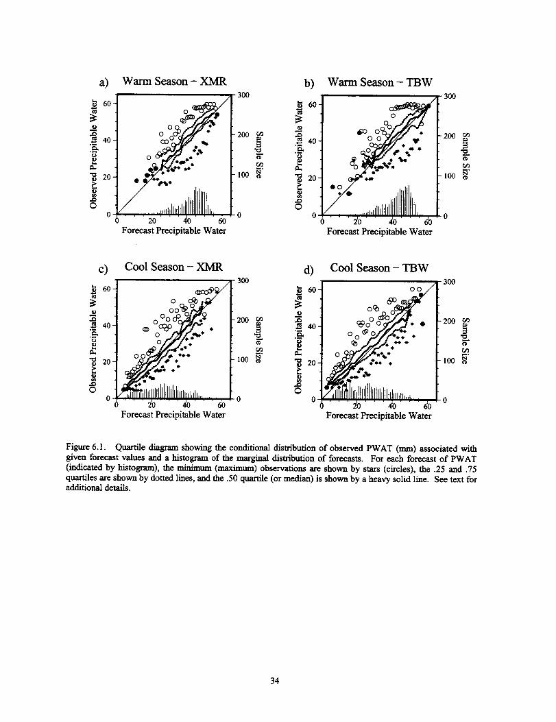
a)

60-

,.o40

o_

.__U

20.

©0

Warm Season - XMR

o°o_J/:_¢f ...,"

°2"_L,..:

Forecast Precipitable Water

300

200

r_

100 _

b) Warm Season- TBW3OO

_ ?o

40 %Od:FAy_ 200

-_ 204 _,,, _,oo

o ......,,,ll_tlI11 I,.06 . • .2,0...4,0...d0 0


_o

c) Cool Season- XMR

o . oOo°_n#._._

_"2o-I °_2:_',/-'.""_ ..t _]/'._-"

o6 ' ' 2'0' ' '4'0' ' '60Forecast Precipitable Water

300

200 r_m

100 ¢_

d) Cool Season - TBW

6o- 6x:__ /o<b o_[

°._o- _ •o o _ °#/f.7 •

"_ _/,/..,4..- •o _T_/_.-¢

20 _Y)._ ¢.- •

6 ' ' ' 2'0 ' ' '4'0' ' _0


30O

2OO r_

100 o

Figure 6.1. Quartile diagram showing the conditional distribution of observed PWAT (ram) associated withgiven forecast values and a histogram of the marginal distribution of forecasts. For each forecast of PWAT(indicated by histogram), the minimum (maximum) observations are shown by stars (circles), the .25 and .75quartiles are shown by dotted lines, and the .50 quartile (or median) is shown by a heavy solid line. See text foradditional details.

34

ID

1,==_

ID

ID

,.OO

a)

10

-5

-10

Warm Season - XMR

0 lt/O0000 00 o(

0_. _ .e •

6"'_-' "6 .... _ .... 1'0'Forecast Lifted Index

300

200 _o

100

b)

10-

x

5

o

,_ -5©

0 -10

Warm Season - TBW

///_ 300

, o o-/o I

•S i. fi''"5' '6"'!_ ....f0" o

Forecast Lifted Index

c)

30-

o

"" 20

10'

r,o,._ O"O

-10

Cool Season - XMR

Joo

_1,I,p......:i...... ,....2'0....3b


d)300

30

200 _ _ 20

_ lO

!00 o o.._ 0©

0 -10_

Cool Season - TBW

(13 r._

o " Ioo to1_ _oo_"

................... 0


Figure 6.2. Quartile diagram showing the conditional distribution of observed lifted index (*C) associated withgiven forecast values and a histogram of the marginal distribution of forecasts. For each forecast of lifted index(indicated by histogram), the minimum (maximum) observations are shown by stars (circles), the .25 and .75

qua.rtiles are shown by dotted lines, and the .50 quartile (or median) is shown by a heavy solid line. See text foradditional details.

35

6.2.3 K-Index

The frequency distribution of warm season K-index forecasts reveals that the indices most often lie in the

range from approximately 28 to 32 °C (Figs. 6.3a, b). The conditional bias within this range is small, but theIQR of about 8 °C reveals substantial day-to-day variability in the forecast errors. The overall sample statistics(Table 6.2) also indicate that the K-index forecasts are nearly unbiased and that the error standard deviations are

large in comparison to the mean. Cool season K-index forecasts are more widely distributed than the warmseason forecasts (Figs. 6.3c, d). When cool season K-index forecasts are negative, they tend to indicate slightlygreater stability than observed soundings. Conversely, when positive, the forecasts tend to indicate slightly lessstability than observed.

6.2.4 Lifted Condensation Level

When air parcels in the forecast soundings are lifted dry adiabatically, they most frequently reach saturationaround 990 to 1000 mb during both warm and cool seasons (Fig. 6.4). The conditional distMbution of theobserved lifted condensation level (LCL) reveals that forecasts are most reliable when the LCL is closer to the

ground. In particular, the large IQR and spread of extreme conditional observations reveals that LCL forecasts

are less refined at lower pressures. During the cool season, the conditional median more closely follows the 45 °reference line, but the distributions still exhibit a large IQR. Since subtle errors in low-level temperature andmoisture will affect the calculation of forecast and observed LCL, it is not surprising that the variability is solarge

6.2.5 Convective Available Potential Energy

During the warm season, the forecast convective available potential energy (CAPE) distribution reveals thatmost forecasts contain nearly zero CAPE and thus are quite stable (Fig. 6.5). When warm season CAPEforecasts are less than about 1500 J kg "I, the conditional median of the observed CAPE distribution is larger thanthe given forecast values (Figs. 6.5a, b). This result indicates that at smaller values, the warm season CAPE

forecasts tend to underestimate the observed instability - a fact which is supported by the negative overallsample bias (Table 6.2). The convective potential of the forecast soundings could be limited by the positive(warm) bias in middle- and upper-tropospheric temperature (Fig. 5.1a) since, in that environment, liI_i air

parcels would require greater energy to attain positive buoyancy. It is noteworthy that even when zero CAPE isforecast the maximum observed CAPE at XMR may exceed 4100 J kg "l during the warm season (3000 J kg "l atTBW). Therefore, warm season CAPE forecasts are susceptible to large errors.

During the cool season, the frequency distribution of forecast CAPE at XMR and TBW reveals that the

Meso-Eta model often predicts a relatively stable environment with many forecast soundings again supportingzero CAPE (Figs. 6.5c, d). Unlike warm season results, the cool season forecasts of small CAPE (i.e., nearzero) exhibit little conditional bias and thus are reliable. However, the wide distribution of the conditionalextreme observations indicates that both warm and cool season CAPE forecasts occasionally suffer large errors.

Given cool season forecasts of large CAPE, a conditional bias becomes evident which suggests theenvironmental instability is overestimated. However, the small sample sizes associated with such forecastsdecrease the robustness of this particular result.

36

ID

©

a) Warm Season - XMR48

32

16

0

-16

o6::°:_ /

°%,;; --'v0 --.-

O0 *®

ot 00 •

:iTiil",It.

s' ''6'' 'f6' ' 's2' ' '_Forecast K-Index

3OO

• 200 r_

N"r_

loo _

0

b) Warm Season - TBW48

32

_ o

-16

o Oo_3_"oc°° it*

o o o ._/'._I"

"°_it. \

o ,t .,.

I.

6' ' ' 6 ' ' 'IZ' ' '3_' ' '4

Forecast K-Index

300

200

_°

1oo g

x

©

c)48

32

16

0

-16

-32

-48--d

Cool Season - XMR

o 6_ o qS_ooo

o °o°jT_/,_o o _..--"/f-/ "°oOJ

• .m tt-

i ' '--_2 "L t6 ' '6' " '1'6' ' '3'2' ' '4t

Forecast K-Index

30O

200

100 N o

©

d)48

32

16

0

-16'

-32

-48

Cool Season - TBW

00_0O0 O0 C_O_0 0

-®o o _o _ oO°S_

__¢////: • :_,_,/./7." "";7_ "-'-

:,,,,:,,,,,I.Forecast K-Index

300

200 r_

r_

100

Figure 6.3. Quartile diagram showing the conditional distribution of observed K-index (°C) associated with

given forecast values and a histogram of the marginal distribution of forecasts. For each forecast of K-index

(indicated by histogram), the minimum (maximum) observations are shown by stars (circles), the .25 and .75

quartiles are shown by dotted lines, and the .50 quartile (or median) is shown by a heavy solid line. See text for

additional details.

37

a) Warm Season - XMR b) Warm Season - TBW

looO _:_00 IOOO-_ 0 0000 _DO_( _iiP/_

200_ _g 200• • •

8o0 ,,,II, l l,,lllll[ ,T, illll t =, o86o 960 ' _0_o o 800860 ' ' ' 960 ' ' ]obo'

Forecast LCL Forecast LCL

c) Cool Season - XMR

° _200

I

, z . ll..,_ooV. ,.T,,,.,.., I. 0

86o ' ' ' 96o ' ' 'logoForecast LCL

d)

1000-

90o-,.oO

8OO

Cool Season - TBW

o o_o°__ioOO_ [/( !

•0 *

. _.-. o° " _'til

Forecast LCL

300

.200 r_

"o

]oo _

Figure 6.4. Quartile diagram showing the conditional distribution of observed LCL (rob) associated with given

forecast values and a histogram of the marginal distribution of forecasts. For each forecast of LCL (indicated by

histogram), the minimum (maximum) observations are shown by stars (circles), the .25 and .75 quartiles are

shown by dotted lines, and the .50 quartile (or median) is shown by a heavy solid line. See text for additionaldetails.

38

a) Warm Season - XMR

6000] ///i 300

45O0qoo °° ° / l:1__o ° o_6_ / I-2oo

30o0 _-

® ® 100 _"

d.........i_ob ' 30bo ,ig06 ' ' 6oh0Forecast CAPE

b)6000

r.r.t 4500 -

<

"_ 3000 -

0 1500.

0

Warm Season - TBW

o

°o°co

I_1I11Illllllllbt, a_ ....

.........ig0b' ' 3doo' ' igo6' '_Forecast CAPE

300

.200 r_

N"

100

ooo

c) Cool Season- XMR d) Cool Season- TBW

Ioo o o / oII o o oco / I- _ oo o ot \o_F f _oo_o o tl _ f_" o o • _",_o01Ooo_/o...[ _ _ ,_0o

o :2Lo"01 'oool"Forecast CAPE Forecast CAPE

Figure 6.5. Quartile diagram showing the conditional distribution of observed CAPE (J kg "1) associated withgiven forecast values and a histogram of the marginal distribution of forecasts. For each forecast of CAPE(indicated by histogram), the minimum (maximum) observations are shown by stars (circles), the .25 and .75qua_rtiles are shown by dotted lines, and the .50 quartile (or median) is shown by a heavy solid line. See text foradditional details.

39

6.2.6 Convective Inhibition

The frequency distributions of convective inhibition (CIN; negative area on a skew-T diagram) are similar

to those of CAPE forecasts (compare Figs. 6.5 and 6.6). Upon first inspection, the simultaneous and regularoccurrence of zero CAPE and CIN may seem in contradiction. However, the explanation is that a closed

positive or negative area is not defined on a thermodynamic diagram if a lifted parcel fails to reach a level offree convection or equilibrium level within its environment. Under this circumstance, the GEMPAK numerical

algorithm assigns zero CAPE and CIN to the sounding as lifted air parcels remain colder (more stable) than the

environmental temperature at all levels. Examination of the warm season data from XMR (not shown) used toconstruct Figs. 6.3a and 6.4a reveals that instances of both zero CAPE and CIN occur in 4.9 and 2.8% of the

available forecasts and observations, respectively. Similarly, 33.9 and 39.3% of the cool season forecasts and

observations at XMR exhibit zero CAPE and CIN. The data for TBW demonslxate a comparable relationship.These results indicate that warm season forecasts at XMR and TBW contain zero CIN and CAPE -- and are

therefore stable -- more often than the observed soundings. During the cool season, instances of zero CAPEand CIN occur regularly, though the observed environment is often more stable than the forecast environment.

While considering all available data, the conditional median of the observations reveals that CIN is

regularly undefforecast during the warm season whenever the forecast CIN is near zero (Figs. 6.6a, b). The factthat warm season forecasts of small (though not necessarily zero) CAPE and CIN both tend to underestimate

their corresponding observations suggests that the model's boundary layer error characteristics are different

from those in the free atmosphere. Indeed, the vertical profiles of temperature and mixing ratio bias (Figs. 5.1and 5.2) each exhibit a shift in sign around the 700 mb level. During the cool season, the CIN forecasts are

conditionally unbiased when near zero (Figs. 6.6c, d). This cool season reliability likely follows from thefrequent occurrence of forecast and observed soundings with zero CAPE and CIN as discussed above. Givenlarger CIN forecasts, the position of the conditional median relative to the 45* reference line indicates that CIN

is usually overforeeast during both the warm and cool seasons. However, since forecasts of large CIN arerelatively uncommon, this conditional bias should be considered cautiously.

6.2.7 Heficity

Positive and negative 0-3 km helicity (Lilly 1986; Davies-Jones et al. 1990) forecasts are nearly evenlydistributed about zero and are thus well refined during both warm and cool seasons at XMR and TBW (Fig.6.7). Helicity forecasts with values near zero are conditionally unbiased. However, the lower slope of theconditional median relative to the 45 ° reference line indicates that the magnitude of the helicity is oftenoverforecast, particularly during the warm season. The overall sample biases (Tables 6.2 and 6.3) are small but

do not fully represent the tendency to overforecast the magnitude of nonzero helicity values as revealed by Fig.6.7. The frequency distribution of cool season helicity forecasts covers nearly double the range of values thatare forecast during the warm'season. The corresponding RMS errors and error standard deviations are also

approximately doubled during the cool season (Tables 6.2 and 6.3). Since helicity is a measure of the vertically

integrated wind shear over the lowest 3 lan of the atmosphere, the larger errors during the cool season are likelyrelated to an increase in forecast and observed wind speeds and corresponding wind shear.

6.2.8 Microburst Day Potential Index

The frequency distribution for Microburst Day Potential Index (MDPI; Wheeler and Roeder 1996) forecastsindicates that most values occur in the range 0.8 to 0.9 during the warm season (Figs. 6.8a, b). The MDPIforecasts are conditionally unbiased and therefore reliable when near 1.0. Given MDPI forecasts less than 1.0,the potential for microburst development is often underforeeast relative to the conditional distribution ofobserved MDPI. Conversely, the microburst potential is typically overestimated as the forecast MDPI exceeds

1.0. Note that at _ the conditional maximum observed MDPI reach 1.25 across nearly the entire range ofgiven forecast values (Fig 6.8a). Since MDPI values above 1.0 support a high probability of wet microburst

development at XMR (Wheeler and Roeder 1996), this result suggests that the model often fails to accuratelypredict the environment conducive for observed microbursts. The slight negative bias in the overall samplestatistics (Table 6.2) supports the tendency to underestimate observed MDPI. During the cool season, the MDPIforecasts cover a wider range of values (more refined) while the slope of the conditional median more closelymatches that of the 45* reference line (more reliable).

40

o°_

_=

o

_D

O

a)450

3o0 -"

150 -

Warm Season - XMR

Z_)O0 0 O/

0 O0 %/_,. 0.00

_ °/°o/

__-_°:,. • "............. 1_0 .... 360 ..... 4:

Forecast Conv. Inhibition

3OO

200

100

b) Warm Season - TBW450 300

fo -

•©

0 1 0 30 400

Forecast Cony. Inhibition

o°_

o

ID

O

c)450

300.

150'

0

Cool Season- XMR

o (It)

o

.............. i_-0- ' '3_0' 4

Forecast Conv. Inhibition

3OO

200 r_

lOO _

d)450

150

0 0

Cool Season - TBW

oooDO 0 0 0 /

0 00/ @

............... 1_0 ..... 360..... 4:

Forecast Cony. Inhibition

3OO

- 200

r_

100 _"

0;0

Figure 6.6. Quartile diagram showing the conditional distribution of observed CIN (J kg d) associated with

given forecast values and a histogram of the marginal distribution of forecasts. For each forecast of CIN(indicated by histogram), the minimum (maximum) observations are shown by stars (circles), the .25 and .75quartiles are shown by dotted lines, and the .50 quartile (or median) is shown by a heavy solid line. See text foradditional details.

41

"d=

s,)

¢_

O

a)300

150

0

-150

-300

Warm Season - XMR

Forecast Helicity

3OO

200 _ .o

]00 _ _,.0

©

oo

b)300

150

0

-150

-300

Warm Season - TBW

O

®00_

_0' '-IE50 0

ForecastHelicity

] ,

3(

3O0

- 200

100

¢/3

E

_°

Nf}

c)6OO

._ 300

.o

0

o

0 -3OO

Cool Season - XMR

-6OO

0000 0 •

/ . .111111 [l ;_

_b ' =3'oh.... 6 3_"iForecast Helicity

300d)6OO

300•200 ou .o

E "_ 0

0 -300

0 -6OO)0

Cool Season - TBW

oy0 000_ 0

0000_ ,_ @

o °_II °

o:/. ?t it- •

/i:i IIli_'''-3oh....6....356 i

ForecastHelicity

3O0

200 o_

]00

Figure 6.7. Quartile diagram showing the conditional distribution of observed helicity (m 2 s"2)associated with

given forecast values and a histogram of the marginal distn'bution of forecasts. For each forecast of helicity(indicated by histogram), the minimum (maximum) observations are shown by stars (circles), the .25 and .75quartiles are shown by dotted lines, and the .50 quartile (or median) is shown by a heavy solid line. See text foradditionaldetails.

42

o

©

a)2

-1

Warm Season - XMR

/..y"..

• IIh,,,.... 6 .... i ....

Forecast MDPI

300

• 200 r_

,oo _" ._©

b) Warm Season - TBW2

--| --

Forecast MDPI

300

200

loo

c)2

0©

Cool Season - XMR

-1

o

0 o

°dP •

.... 2

Forecast MDPI

300d)

2

200 r_ _ 1

_oo_" ._ o©

-1-1

Cool Season - TBW

O ®

o * *

'''6 .... i'

Forecast MDPI

300

.200t_

loo g

Figure 6.8. Quartile diagram showing the conditional distribution of observed MDPI associated with givenforecast values and a histogram of the marginal distribution of forecasts. For each forecast of MDPI (indicatedby histogram), the minimum (maximum) observations are shown by stars (circles), the .25 and .75 quartiles are

shown by dotted lines, and the .50 quartile (or median) is shown by a heavy solid line. See text for additionaldetails.

43

7.0 850 to 500-mb Layer-Averages

The warm and cool season bias, RMS error, and error standard deviation for 1000- to 850-rob thickness and

850- to 500-rob layer-averaged winds and relative humidity are presented for XMR, TBW, and EDW in Table

7.1. The statistics were calculated as requested by the original evaluation protocol (Table 1.1). As withconvective parameters, calculations were performed using all available data from both the 0300 and 1500 UTC

model runs and corresponding observations.

The RMS errors for the 1000- to 850-mb thickness are less than 12 m during both warm and cool seasons atXMR and TBW. The thickness errors are not indicated for EDW because the surface pressure at that location is

often less than 1000 mb. Forecast biases for the 850- to 500-rob layer-averaged relative humidity are less than±2% except at EDW during the cool season. Notably, these biases arc smaller than the 2.5% observational

uncertainty associated with rawinsonde observations of relative humidity (Almert 1991). Wind speed biases aresmall compared to the error standard deviation and RMS errors. These results are consistent with those shown

previously in Fig. 5.4 and further indicate that the greater portion of wind speed errors are obtained from

nonsystematic sources. Wind direction errors behave similarly, with near zero biases and relatively larger RMSerrors and error standard deviations.

Table 7.1. Warm and cool season bias, RMS error, and error standard deviation for 1000- to

850-rob thickness and 850- to 500-rob layer-averaged relative humidity, wind speed, and winddirection.

Thickness(m)

Relative Humidity (%)

Wind Speed (m s"I)

Wind Direction (0)

Bias

Warm

XMR

TBW

EDW

XMR

TBW

EDW

XMR

TBW

EDW

XMR .32

TBW 3.72

EDW -6.37

RMS Error Error Std. Dev.

Cool Warm Cool Warm Cool

-3.02 7.27

1.11 6.31

-.51 .81

1.24 -1.37

1.32 3.38

.13 -.23

-.03 -.13

-.88 -.19

.01

1.76

-4.69

10.31 11.77

8.37 10.57

11.63 13.62

12.09 12.87

8.03 12.62

2.09 2.01

1.97 2.14

2.20 2.75

42.62 22.97

45.83 24.34

38.04 38.64

9.86 9.26

8.29 8.48

I1.62 13.60

12.02 12.79

7.92 12.16

2.08 2.00

1.97 2.14

2.02 2.74

42.62 22.97

45.68 24.28

37.50 38.35

8.0 Wind Regime Stratification

Within each seasonal evaluation period, the original evaluation protocol specified that the statisticalverification would be stratified by average wind direction in the layer from 950 to 600 nab using seven wind

regimes following HoNe et al. (1992). This type of stratification was designed to determine if the model forecast

errors are sensitive to specific flow regimes as defined by the layer-averaged wind directions. During the initialevaluation period in 1996, it was determined that insufficient numbers of forecast/observation pairs wereavailable within each of the seven wind regimes. The small sample sizes made it difficult to draw meaningfulconclusions regarding error characteristics as a function of flow regime (Panofsky and Brier 1958). As asimplification, westerly and easterly regimes were defined based on winds that are approximately perpendicularto Florida's east coast. In particular, the 950- to 600-rob layer-averaged winds are considered westerly between158 ° and 338" and easterly outside that range. As reported by MN97, this stratification also did not reveal anysubstantial differences in the forecast error characteristics under easterly or westerly flow.

44

The extensionof theevaluationfora second consecutiveyearhelpsmeliorate thedifficultyof insufficient

sample sizes. Again, the statisticswere stratifiedby the 950 to 600 mb layer averaged wind direction.

Examinationof the stratifiedstatistics(notshown) againdid not revealany substantialdifferencesinforecast

errorfrom one regime tothenext.On average,theobservationsdidindicatesubtle,yetexpectedchangesbased

on wind direction.However, theMcso-Eta model demonstratesthecapability,on average,tofollowshiftsinthe

mean observationsas a functionofwind regime. Therefore,themodel's overallforecasterrorcharacteristics

remain mostly unchanged regardlessof wind regime. In most cases,the varianceof the errorsunder the

differentregimesare similar.This resultsuggeststhatthe day-to-dayvariationsinthe forecasterrorsmay be

more difficulttoanticipatethanchangesintheoverallerrorcharacteristicsfordifferentregimes.

9.0 Summary of Subjective Forecast Value

Statisticalverificationofpointforecastsisa stringentmeasure ofmodel performance.However, when used

alone,the statisticsarenot enough to quantifytheoverallvaluethatmodel guidance may add to the forecast

process.This isespeciallytrucformodels with enhanced spatialand temporalresolutionthatmay be capableof

generatingmeteorologicallyconsistent,though not necessarilyaccuratemesoscale weather phenomena (e.g.

Cortinasand Stcnsrud 1995). With thisinmind, the AMU performed a subjectiveverificationof Meso-Eta

model forecaststo help quantifythe added valuethatcannotbe inferredsolelyfrom an objectiveevaluation.

Resultsfrom theAMU's subjectiveverificationoftheMeso-Eta model overtheFloridapeninsulaare discussed

intheearlierreporton theMeso-Eta evaluation(MN97) but are summarized here forcompleteness.Interested

readersare encouragedtocontacttheAMU fora copy ofthecompletereport.

The subjectiveevaluationincluded warm-season forecastexercisesand phenomenological verification

focusingprimarilyon limitedcase studiesand seasonalevaluationsof sea breezes,thunderstorms,and cold

fronts.Some resultsfrom the subjectiveevaluationthatmay be importantfor operationalforecastconcerns

includethe following.

Sea-breeze case studies reveal that the model generates a dynamically consistent,thermally direct circulation over the Florida peninsula, although at a larger scale thanobserved. Seasonal verification of sea breezes indicates that the model forecasts the

occurrence of east and/or west coast sea breezes roughly 50% of the time they areobserved.

Thunderstorm verification reveals that the meso-eta model is capable of predicting areasof organized convection over portions of the Florida peninsula, particularly during thelate afternoon hours. On the other hand, the model is also subject to subtle errors that canlead to incorrect forecasts of warm season convective precipitation. In particular, the

model often generates excessive rainfall during the morning hours and is not capable ofaccurately forecasting individual thunderstorms.

Verification of cold fronts during the cool season reveals that the model is capable offorecasting a majority of cold frontal passages through east central Florida to within + 1 hof observed frontal passage.

Seasonal evaluations of sea breezes, thunderstorms, and cold fronts are designed to quantify howconsistently the Meso-Eta model provides value in forecasts of these phenomena. Results suggest that the model

forecasts over central Florida may have more value during the cool season. This statement is based on the factthat the meso-eta model resolution is not sufficient to resolve the small-scale details of sea and fiver/lake breeze

circulations, thunderstorm outflow boundaries, and other phenomena which play a dominant role in determiningthe short-term evolution of weather over east central Florida during the warm season.

45

10.0 Summary and Lessons Learned

From May 1996 through January 1998, the AMU conducted warm- and cool-season evaluations of Meso-Eta surface and upper-air point forecast accuracy at XMR, TBW, and EDW. These three locations wereselected because they are important for 45WS, NWS MLB, and SMG operational concerns. Each warm- and

cool-season verification period extends from May through August and October through January, respectively.By extending the evaluation for a second consecutive year, it was possible to identify statistically significantchanges in the error characteristics which developed in response to the February and August 1997 model

updates (BL97; EMC 1997). The twin-season comparison of forecast accuracy is helpful for model users byhighlighting the model's characteristic strengths and weaknesses before and after the incorporation of model

updates. Such results are also helpful for model development efforts and emphasize the need for ongoinganalysis of model errors at specific locations.

10.1 Surface Results

The error characteristics for Meso-Eta point forecasts of surface parameters are summarized in Tables 4.1-

4.3. The surface error statistics are difficult to generalize because they vary widely by location, season, and timeof day. The results are utilized most effectively by considering the model biases for each parameter separatelyand making the appropriate adjustments.

The random error component reveals substantial day-to-day variability in forecast accuracy. For manyparameters, the random errors are larger than the corresponding biases, or systematic model errors. The random

errors are caused primarily by the model's inability to resolve localized phenomena such as wind gusts,temperature gradients, or the effects of thunderstorms. While it is possible to partially adjust for model biases, it

is much more difficult to accommodate the variability in forecast errors on any given day. It might help tocompare current observations with the latest forecast guidance and make appropriate adjustments.

As modeling systems such as the Meso-Eta attain greater resolution, they tend to exhibit smaller biases and

larger error standard deviations. The nonsystematic, random error component associated with any model'sinability to resolve local phenomena prevents perfect forecast guidance. However, the relatively minor biasesindicate that on average, point forecasts provide useful guidance for the basic seus_le weather variablesconsidered here.

Results shown in sections 4.2 and 4.3 indicate that changes to the model's physical parameterizationsproduced identifiable and statistically significant changes in forecast accuracy at each location. Some changesenhanced forecast accuracy while others created larger errors. It is important that model users maintain

awareness of ongoing model changes. Such changes are likely to modify the basic error characteristics,particularly near the surface.

10.2 Upper-air Results

Results from the upper-air verification are summarized in Tables 5.1 and 5.2. On average, the forecastsoundings at XMR and TBW during the warm season are too stable. The height of the lower troposphericinversion at XMR and TBW was misrepresented during the cool season. Forecast biases for wind speed anddirection are small at all three locations, but the random error component dominates the day-to-day variability.

Given this variability, real-time assessment of forecast accuracy is necessary on any given day to help usersdetermine ff the model forecasts are consistent with current observations.

The statistics did not reveal annual changes in forecast errors that could be atwibuted solely to the February

and August 1997 model updates. The model's systematic error growth during the forecast cycle is minimal(section 5.3), implying that all data could be combined into a single dataset regardless of duration. Moreover,since error growth is minimal, the characteristics outlined in Tables 5.1 and 5.2 apply, on average, at any timeduring the forecast period. This generality does not apply to the surface data where error characteristics variedwith time of day.

46

10.3 Convective Index Results

Convective index results are summarized in section 6.1. In general, the results suggest that day-to-dayfluctuations in observed convective indices at XMR and TBW are not well represented by the Meso-Eta modelthroughout the warm season. In addition, the conditional quartile diagrams suggest that forecasts occasionallysuffer large errors in representing the true convective potential of the atmosphere. The forecast biases and

variability of the errors are confirmed by the overall sample statistics (Tables 6.2 and 6.3) and support the notionthat much of the error at upper levels is largely nonsystematic in nature. The convective index forecasts aremost reliable overall during the cool season when, under normal circumstances, they provide little added value

for most operational forecasting applications.

10.4 Layer Averages and Wind Regime Stratification

The I000- to 850-rob thickness and 850- to 500-mb layer averaged relative humidity and winds indicate thatbiases in Meso-Eta forecasts for these parameters are small relative to the error standard deviations. This resultsuggests that the middle tropospheric errors are dominated by day-to-day variations in the difference between

the forecasts and observations. Stratification of errors by the 950- to 600-mb wind direction does not reveal anysubstantial changes in error characteristics, and further indicates that the day-to-day variations in the forecasterrors may be more difficult to anticipate than more general changes in the overall error characteristics under

different wind regimes.

10.5 Lessons and Recommendations

The AMU's statistical evaluation of Meso-Eta forecast accuracy identified a few biases that may result frominadequate parameterization of physical processes near the surface. Since the model bias or systematic error

generally is small, most of the total model error results from day-to-day variability in the forecasts and/orobservations. To some extent, these nonsystematic errors reflect the variability in point observations that samplespatial and temporal scales of atmospheric phenomena which cannot be resolved by the model. On average,Meso-Eta point forecasts may provide useful guidance for predicting the evolution of the larger scaleenvironment. A more substantial challenge facing model users in real time is the discrimination ofnonsystematic errors that could inflate the total forecast error.

It is important that forecasters maintain an ongoing awareness of model updates and the effects that suchchanges will have on point forecast accuracy within their area of responsibility. While model updates aregenerally well tested and designed to improve forecast accuracy, the results shown here demonstrate that the

desired effects do not always yield the expected improvements at every location. This may become particularlytrue as national-scale, operational models with greater horizontal and vertical resolutions are able to forecastexplicitly the complex processes that occur within the PBL. In recent years, information documenting modelupdates has been made available regularly on the interact. Indeed, much of the information needed for writingthis report and maintaining an understanding the model changes was obtained from an interact FAQ writtenexpressly for this purpose (EMC 1997). As forecasters discover localized model deficiencies through ongoingreal-time statistical verification strategies, results should be documented regularly and shared with model

developers. As expressed by Manning and Davis (1997), "These statistics would provide additional informationto model users and alert model developers to those research areas that need more attention". The additional andcomplementary need for subjective verification strategies in mesoscale models is discussed in the earlier report

by M'N97.

On 9 February 1998, NCEP upgraded the horizontal resolution of the "early" Eta model from 48 to 32 kin,with an increase in vertical resolution from 38 to 45 levels (Rogers et al. 1997). In addition, a three-dimensionaivariational analysis scheme was implemented along with the use of a "partial" continuous Eta Data AssimilationCycle. Aside from the differences in data assimilation methods at the time of this writing, this version of the"early" Eta is similar in resolution and dynamics to the Meso-Eta model version evaluated here. Therefore theobjective verification results presented here for XMR, TBW and EDW and the subjective verification resultspresented in MN97 should establish a reasonable benchmark from which model users and developers may

pursue ongoing Eta model verification strategies in the future.

47

11.0 References

Ahnert, P. R., 1991: Precision and compatibility of National Weather Service upper air measurements.Preprints, Seventh Syrup. on Meteorological Observations and Instrumentation, New Orleans, LA, Amer.Meteor. Sot., 221-226.

Baldwin, M. E., and S. D. Hrebenach, 1998: Experiments with bias-corrected temperature guidance usingNCEP's mesoseale Eta model. Preprints, 16th Conf. on Weather Analysis and Forecasting, Phoenix, AZ,Amer. Meteor. Sot., 388-389.

Betts, A. K., F. Chen, K. E. Mitchell, and Z. I. Janjic, 1997: Assessment of the land surface and boundary layer

models in two operational versions of the NCEP Eta model using FIFE data. Mon. Wea. Rev., 125, 2896-2916.

Black, T. L., 1994: The new NMC mesoscale Eta model: description and forecast examples. Wea. Forecasting,9, 265-278.

, M. Baldwin, K. Brill, F. Chen, G. DiMego, Z. Janjic, G. Manikin, F. Mesinger, K. Mitchell, E. Rogers,and Q. Zhao, 1997: Changes to the Eta forecast systems. NWS Technical Procedures Bulletin 441,NOAA/NWS, 31 pp. [Available from National Weather Service, Office of Meteorology, 1325 East-WestHighway, Silver Spring, MD 20910.]

Carter, G. M., J. P. Dallavalle, and H. R. Glahn, 1989: Statistical forecasts based on the National MeteorologicalCenter's numerical weather prediction system. Wea. Forecasting, 4, 401-412.

Chen, F., K. Mitchell, J. Schaake, Y. Xue, H.-L. Pan, V. Koren, Q. Duma, and A. Betts, 1996: Modeling of land-surface evaporation by four schemes and comparison with FIFE results. J. Geophys. Res., 101, 7251-7268.

Cortinas, J. V., Jr., and D. J. Stensrud, 1995: The importance of understanding mesoscale modelparameterization schemes for weather forecasting. Wea. Forecasting, 10, 716-740.

Davies-Jones, R., D. Burgess, and M. Foster, 1990: Test of helicity as a tornado forecast parameter. Preprints,16 th Conf. on Severe Local Storms, Kananaskis Park, Alberta, Canada, Amer. Meteor. Soc., 588-592.

desJardins, M. L., S. Jacobs, D. Plummer, and S. Schotz, 1997: N-AWIPS: AWIPS at the National Centers forEnvironmental Prediction. Preprints, 13 th International Conf. on Interactive Information and ProcessingSystems, Long Beach, CA, Amer. Meteor. Sot., 296-298.

EMC, cited 1997: Environmental Modeling Center: Mesoscale Modeling Branch FAQ. [Available on-line fromhttp://nic.f134.noaa.gov:8000/researeh/FAQ-eta.html.]

Glahn, H. R., and D. A. Lowry, 1972: The use of model output statistics (MOS) in objective weatherforecasting, or. AppL Meteor., 11, 1203-1211.

Hoehne, W. E., 1980: Precision of National Weather Service Upper Air Measurements. NOAA Tech. Memo.NWS T&ED-16.

Holle, R. L., A. I. Watson, R. E. Lopez, K. W. Howard, 1L Ortiz, and L. Li, 1992: Meteorological studies toimprove short-range forecasting of lightning�thunderstorms within the Kennedy Space Center area. FinalReport for Memorandum of Agreement Between the Office of Space Flight, NASA and the National SevereStorms Laboratory, NOAA, Boulder, CO, 91 pp.

Homleid, M., 1995: Diurnal corrections of short-term surface temperature forecasts using the Kalman filter.Wea. Forecasting, 10, 689-707.

48

Janjic,Z. I., 1994:Thestep-mountainEtacoordinate model: Further developments of the convection, viscoussublayer, and turbulence closure schemes. Mon. Wea. Rev., 122, 927-945.

, 1996a: The Mellor-Yamada level 2.5 turbulence closure scheme in the NCEP Eta model. Research

Activities in Atmospheric and Oceanic Modeling, WMO, Geneva, CAS/JSC WGNE, 4.14-4.15. [Availablefrom World Meteorological Organization, Case Postale 2300, CH-1211 Geneva, Switzerland.]

, 1996b: The surface layer parameterization in the NCEP Eta Model. Research Activities in Atmosphericand Oceanic Modeling, WMO, Geneva, CAS/JSC WGNE, 4.16-4.17. [Available from World

Meteorological Organization, Case Postale 2300, CH-1211 Geneva, Switzerland.]

, 1996c: The surface layer in the NCEP Eta model. Preprints, llth Conf. on Numerical WeatherPrediction, Norfolk, VA, Amer. Meteor. Soc., 354-355.

Lilly, D. K. 1986: The structure, energetics and propagation of rotating convective storms. Part II: Helicity and

storm stabilization. J. Atmos. Sci., 43, 126-140.

Manning, K. W. and C. A. Davis, 1997: Verification and sensitivity experiments for the WISP95 MM5forecasts. Wea. Forecasting, 12, 719-735.

Manobianco, J. M., and P. A. Nutter, 1997: Evaluation of the 29-kin Eta Model for Weather Support to theUnited States Space Program. NASA Contractor Report CR-205409, Kennedy Space Center, FL, 91 pp.[Available from ENSCO, Inc., 1980 N. Atlantic Ave., Cocoa Beach, FL 32931.]

McPherson, R. D., 1994: The National Centers for Environmental Prediction: Operational climate, ocean, and

weather prediction for the 21st century. Bull. Amer. Meteor. Soc., 75, 363-373.

Mesinger, F., 1996: Improvements in quantitative precipitation forecasts with the Eta regional model at theNational Centers for Environmental Prediction: The 48-km upgrade. Bull. Amer. Meteor. Soc., 11, 2637-2649.

Murphy, A. H., 1988: Skill scores based on the mean square error and their relationships to the correlationcoefficient. Mon. Wea. Rev., 116, 2417-2424.

--, B. G. Brown, and Y. Chen, 1989: Diagnostic verification of temperature forecasts. Wea. Forecasting, 4,485-501.

Panofsky, H. A., and G. W. Brier, 1958: Some Applications of Statistics to Meteorology. Pennsylvania StateUniversity, University Park, 224 pp.

Rogers, E., D. G. Deaven, and G. J. DiMego, 1995: The regional analysis system for the operational "early" Etamodel: Original 80-kin configuration and recent changes. Wea. Forecasting, 10, 810-825.

--, T. L. Black, D. G. Deaven, and G. J. DiMego, 1996: Changes to the operational "early" Eta

analysis/forecast system at the National Centers for Environmental Prediction. Wea. Forecasting, 11, 391-413.

--, M. Baldwin, T. Black, K. Brill, F. Chen, G. DiMego, J. Gerrity, G. Manikin, F. Mesinger, K. Mitchell, D.Parrish, Q. Zhao, 1997: Changes to the NCEP Operational "Early" Eta Analysis / Forecast System. NWS

Technical Procedures Bulletin 447, NOAA/NWS. [Available from National Weather Service, Office ofMeteorology, 1325 East-West Highway, Silver Spring, MD 20910.]

Stensrud, D. J., and J. A. Skindlov, 1996: Gridpoint predictions of high temperature from a mesoscale model.

Wea. Forecasting, 11, 103-110.

Tukey, J. W. 1977: Exploratory Data Analysis. Addison-Wesley, Reading, MA.

49

Wallace,J.M.,and P. V. Hobbs, 1977: Atmospheric Science: An Introductory Survey. Academic Press, 467 pp.

Walpole, R. E., and R. H. Meyers, 1989: Probability and Statistics for Engineers and Scientists. Macmillan,765 pp.

Wheeler, M. M., and W. P. Roeder, 1996: Forecasting wet microburst on the Central Florida Atlantic coast in

support of the United States Space Program. Preprints, 18th Conf. on Severe Local Storms, San Francisco,CA, Amer. Meteor. So¢., 654-658.

Wilks, D. S., 1995: StatisticalMethods in the Atmospheric Sciences. Academic Press, 467 pp.

Zhao, Q., T. L. Black, and M. E. Baldwin, 1997: Implementation of the cloud prediction scheme in the Eta

model at NCEP. Wea. Forecasting, 12, 697-712.

5O

Appendix A

EtaModelOverview

The primary mesoscale modeling efforts at NCEP are focused on the development of the Eta model (Rogerset al. 1995). The original version of the Eta model with a horizontal resolution of 80 km and 38 vertical layersreplaced the Limited-Area Fine Mesh model in June 1993 (Black 1994). In October 1995, NCEP increased the

horizontal resolution of the operational "early" Eta model from 80 km to 48 kin. At the same time, a cloudprediction scheme (Zhao et al. 1997) was implemented and initial analyses were produced using the Eta DataAssimilation System (Rogers et al. 1996). In August 1995, NCEP also began running a mesoscale version of the

Eta (meso-eta) model with a horizontal resolution of 29 km and 50 vertical layers (Mesinger 1996). Followingmodel upgrades on 31 January 1996 (Chen et al. 1996; Janjic 1996a; Janjic 1996b; Janjic 1996c; Betts et al.

1997), the "early" and Meso-Eta model configurations became identical except for resolution and dataassimilation procedures. The relevant numerics and physics of the Eta model are summarized in Table A. 1.

NCEP implemented two major changes to the Eta model's physical parameterizations during the AMU'sobjective evaluation period. On 18 February 1997, components of the soil, cloud, and radiation packages were

updated in both models (Betts et al. 1997; Black et al. 1997; EMC 1997). These modifications were designed tohelp control excessive net shortwave radiation at the ground that led indirectly to a bias in the diurnal range ofsurface temperatures, excessive mixing of the planetary boundary layer (PBL), and a negative bias in surfacedew point temperatures. On 19 August 1997, calculation of the model's PBL depth was adjusted to correct for

an underestimation of vertical moisture transport out of the lowest model layers (EMC 1997). A portion of theresults shown below indicate that combined effects of these changes led to identifiable and statisticallysignificant changes in forecast accuracy for a few selected parameters.

Table A. 1. Eta model attributes from Black (1994), Janjic (1994), and

Ro_ers et al. (1996).Dynamics

Model top = 25 mbTime step = 72 s

Semi-staggered Arakawa E-gridGravity wave coupling scheme

Silhouette-mean orography

Split-explicit time differencingPhysics

Explicit grid-scale cloud and precipitationModified Betts-MiUer convective adjustment

Mellor-Yamada (2.5) for free atmosphere vertical turbulent exchangeMellor-Yamada (2.0) near ground

Geophysical Fluid Dynamics Laboratory radiation scheme

Viscous subla:cer over water

51

Appendix B

Statistical Verification Techniques

The statistical measures used here to quantify model forecast errors are the bias, root mean square (RMS)

error, and standard deviation. If F represents any of the parameters under consideration for a given time and

vertical level, then forecast error is defined as _' = Of - _o where the subscripts fand o denote forecast and

observed quantities, respectively. Given N valid pairs of forecasts and observations, the bias is computed as

03.1),

theRMS erroriscomputed as

I_S N ]1/2RMSE = [MSE] I/2 = /_=!((1); )203.2),

and the standard deviation of the errors is computed as

03.3).

In equation 03.3), N is used rather than N-1 so that a decomposition following Murphy (1988, Eq. 9) couldbe applied to the MSE:

MSE = "_,2 + O_203.4).

Therefore, the total model error consists of contributions from model biases (-O'2) and random variations in the

forecast and/or observed data (o .'2 ). Note that if the model bias or systematic error is small, most of the MSE is

due to random, nonsystematic type variability in the errors. Murphy's (1988) decomposition of the MSEconsidered individually the error contributions from the model bias and from the sample variances and

covariance of the forecasts and observations. Here, Eq. B.4 represents an algebraic simplification of thatdecomposition and quantifies the portion of the MSE that is due to the bias and the variance of the forecasterrors.

Tests are applied to the surface data in order to determine ff model updates led to statistically significantchanges in mean forecast error between the 1996 and 1997 warm and cool season periods. Following theCentral Limit Theorem as described in most statistical texts, it is assumed that the sampling distribution for the

difference in mean forecast error between 1996 and 1997 is approximately normal. Sample sizes of O(100) foreach season enable use of the standardized Z statistic where

m

03.5),

the variance inflation factor, _ = (I + r)/(1 - r), and r is the lag-I day autoeorrelation for each seasonal time

series of data. The variance inflation factor helps prevent the overestimation of Z by adjusting the variance ofthe sampling distribution to account for the influence of serial dependence, or day-to-day persistence, within theseasonal time series average 0Vilks 1995). A two-tailed comparison of Z to the normal distribution using a 99%confidence level has critical values of±2.58 (Walpole and Meyers 1989). Calculated values of Z that lie outside

this critical range indicate that the data are able to support a statistically significant difference between the 1996and 1997 seasonal mean forecast errors.

52

Thestatisticalsignificanceof upper-level systematic error growth from early to latter stages of the forecastcycle is determined using a paired Z statistic. The paired Z statistic normalizes the seasonally averaged

difference in forecast error between two times during the ith cycle by the associated sample standard deviation.The covariance between errors in the early and latter stages of the forecast is included because the parametersfrom the ith cycle are not independent and do not necessarily have equal variances 0Nalpole and Meyers 1989).

Here, the paired Z statistic is denoted by Z' where

N t

Z'

The subscripts 1 and 2 denote variables from the ith forecast cycle verifying at 6-9 h and 30-33 h, respectively.

The times used for verification are separated by 24 h and are taken at forecast durations that vary slightly

according to balloon release times. Other notations are as above except that (o-'t2) 2 denotes the sample

covariance. Again using a 99% confidence level, values of Z' that lie outside the critical values of ±2.58

indicate that the data are able to support a statistically significant 24-h systematic error growth in the upper-airforecasts.

53

Appendix C

Upper Level Wind Errors Listed as a Function of Height

As specified in the original evaluation protocol, objective verification results are listed as a function ofgeopotential height. The wind variables are of primary interest for applications to Shuttle flight rules and are

listed in tabular format for direct reference. Plots of wind speed and direction errors as a function of height (notshown) exhibit exactly the same characteristics as those shown in Figs. 5.3 and 5.4. Therefore, the discussions

in sections 5.3 and 5.4 are applicable to the wind speed and direction errors listed below. Although results for uand v wind components are not discussed in previous sections they are generally consistent with results for wind

speed. As discussed at the beginning of section 5, substantial differences do not appear to exist between the0300 and 1500 UTC forecast cycles. Moreover, the statistics do not reveal any obvious differences when theresults are stratified by the 950- to 600-mb layer-averaged wind direction. For these reasons, all available datafrom each season are included in the statistical calculations below. Results from TBW are not shown but are m

fact very similar to those shown below for XMR. At EDW, results below 3000 ft are not available since thelowest level of data extracted from model point forecasts at that location is at an elevation of 3238 ft.

54

TableC. 1. Warm season biases for wind variables at XMR and EDW as a function of geopotential height.

Height (lift):

I

2

3

5

10

12

20

25

28

35

38

45

50

55

60

70

U-wind (ms -1)

XMR EDW

.21 ---li -.14 ---II -.44 ---l' -.64 -.80

-.02 -. 15Ii .18 -.04

-.52 -.71

-.46 -.98

-. 11 -.62

.53 -.42

.68 -.38

.90 -.75

, 1.20 -.90

1.70 1.09

3.50 2.89

8.15 5.04

V-wind (ms "I)

XMR EDW

-.27 --

.13 ---

.41 ---

.65 -.92

-.40 .27

-.60 .26

-.20 1.00

-.37 1.25

-.39 1.53

-.30 1.29

.04 1.24

.68 1.35

.28 .40

.34 .71

1.35 -.65

4.29 -.59

Wind Speed (ms "l)

XMR EDW

.16 ---

.48 ---

.47 --

.33 -1.24

.07 -1.04

-.01 -.89

-.34 .05

-.22 -.44

-. 13 -.24

.16 -.15

-.01 .02

.48 -.79

.85 -1.05

.34 .01

-.72 -.23

-3.66 -1.70

Wind Direction(o)

XMR EDW

1.37 ---

1.31 ---

3.05 ---

-6.45 -2.62

-1.04 -6.91

2.17 -7.53

-.72 -9.22

-1.45 -10.29

1.14 -8.59

-1.25 -5.22

-2.65 -4.05

-4.85 -2.81

-4.89 -1.91

-3.21 -.39

3.27 10.64

35.63 9.87

Table C.2. Cool season biases for wind variables at XMR and EDW as a function of _eopotential heig_ht.

Height (kft):

1

2

3

5

10

12

20

25

28

35

38

45

5O

55

60

7O

U-wind (ms "l)

XMR EDW

-.16 ---

-.67 ---

-.80 --

-.65 -2.07

-.33 -1.03

-.41 -.79

-.71 .95

-.37 1.18

-.43 1.75

-.10 2.27

-.18 2.18

.70 2.96

.45 i.80

1.75 2.09

5.96 2.83

9.47 4.51

V-wind (ms "])

XMR EDW

-.28 ---

-.12 --

.25 ---

.46 .05

-.07 1.15

-.18 1.74

-.34 2.11

-.43 2.44

-.25 2.57

.06 2.73

.38 2.71

.63 1.01

-.05 2.42

-.34 .33

-.02 .38

1.54 - 1.94

Wind Speed (m $-1)

XMR EDW

.34 ---

.86 ---

.53 --

-.03 -.93

-.22 -.45

-.36 -.59

-.66 .75

-.48 .68

-.54 1.87

-.39 1.43

-.32 1.61

.84 2.31

.27 1.23

1.89 1.85

5.16 2.76

7.14 4.47

Wind Direction(o)

XMR EDW

-.23 w

.23 --

3.41 --

.32 -.20

-.10 -4.82

.44 -2.29

1.21 -7.02

1.76 -8.70

1.21 -7.29

-.17 -7.35

-1.34 -6.48

-1.I0 -3.88

-.12 -7.11

-1.03 -5.79

-5.16 .4.43

-.12 4.69

55

TableC.3.

Height

I

2

3

5

10

12

20

25

28

35

38

45

50

55

60

70

(lift):

Warm seasonRMS errorsforwind variablesatXMR and EDW asa functionofgeopotential

h ie t.U-wind (ms "l) V-wind (ms "l) Wind Speed (m sq) Wind Direction (o)

XMR EDW XMR EDW

3.10

2.90 ---

2.93 --

3.18 3.14

2.85 3.01

2.89 3.25

2.86 3.65

3.12 3.77

3.33 4.17

4.62 4.46

5.21 4.83

5.41 4.92

4.40 4.05

3.85 4.09

3.56 3.58

5.69 3.22

XMR EDW

2.66 ---

2.74 ---

2.80

2.93 3.78

2.90 2.93

2.99 3.32

2.75 3.48

3.01 3.62

3.55 3.52

4.78 4.47

5.33 4.71

5.26 4.50

4.67 3.98

3.89 3.89

3.94 3.60

6.17 4.94

XMR EDW

53.20 --

51.81 --

54.56 ---

57.16 47.05

49.62 48.27

48.97 43.23

45.19 34.39

44.90 27.68

44.00 26.99

42.91 23.54

40.93 19.14

37.65 20.37

42.33 24.77

52.14 37.31

57.40 55.59

82.92 59.58

3.01

2.87 m

2.85 --

3.05 3.95

3.01 3.26

3.00 3.38

3.09 3.70

3.42 3.87

3.81 3.49

4.99 4.33

5.57 4.52

5.36 4.13

4.80 3.77

4.37 4.07

4.72 4.88

8.88 6.05

Table C.4. Cool season RMS errors for wind variables at XMR and EDW a function of geopotential height

(lift): U-wind (m s"t) V-wind (ms "t) Wind Speed (m sq ) Wind Direction (o)Height

1

2

3

5

10

12

20

25

28

35

38

45

5O

55

60

70

XMR EDW

2.67

2.66

3.01 ---

3.33 4.38

2.90 4.30

2.95 4.87

3.64 5.50

3.76 6.99

XMR EDW

.04 _m_

3.16 ---

3.13

3.37 3.23

3.26 4.53

3.18 4.96

3.61 6.98

3.97 7.89

XMR EDW

2.64 m

2.84

3.04 m

3.27 3.68

2.89 3.81

2.92 4.22

3.62 5.72

3.75 6.90

XMR EDW

38.11 --

38.52 --

40.01

40.13 61.70

32.33 46.99

30.83 44.16

23.51 31.21

20.17 31.57

16.09 26.88

12.61 23.51

12.76 24.23

11.41 21.71

11.82 23.85

16.79 27.62

37.16 22.88

68.87 33.26

4.08 7.10

5.57 7.99

5.16 7.94

5.11 8.24

5.22 6.52

4.53 5.70

7.08 6.08

10.15 6.95

4.09 8.04

5.26 10.33

5.06 9.90

5.71 7.21

5.17 6.60

4.33 6.84

4.13 7.41

5.56 8.05

5,14 8.81

5.23 7.51

5.11 5.99

4.46 5.73

3.88 4.91

4.57 5.04

6.50 6.30

8.81 6.89

56

TableC.5.

Height(lift):

1235

101220252835384550556070

WarmseasonerrorstandarddeviationsforwindvariablesatXMRand EDW as a function of

geopotential height.

U-wind (ms "l) V-wind (ms "l) Wind Speed (ms "t) ] Wind Direction (o)

XMR EDW XMR EDW

3.09 --

2.90 --

2.90

3.12 3.01

2.83 3.00

2.83 3.24

2.86 3.51

3.10 3.56

3.31 3.88

4.61 4.26

5.21 4.67

5.37 4.73

4.39 4.03

3.83 4.02

3.30 3.52

3.74 3.17

XMR EDW

2.66 --

2.70 --

2.76

2.91 3.57

2.90 2.74

2.99 3.20

2.73 3.48

3.00 3.59

3.55 3.51

4.77 4.47

5.33 4.71

5.24 4.43

4.60 3.84

3.88 3.89

3.87 3.60

4.96 4.63

XMR EDW

53.18 ---

51.79 --

54.48

56.80 46.98

49.61 47.78

48.92 42.57

45.18 33.13

44.88 25.69

43.99 25.59

42.89 22.96

40.84 18.70

37.33 20.18

42.05 24.69

52.04 37.31

57.31 54.56

74.87 58.76

3.00

2.87 ---

2.82 --

2.98 3.87

3.01 3.26

2.99 3.38

3.05 3.63

3.39 3.74

3.81 3.43

4.96 4.31

5.53 4.50

5.29 4.06

4.65 3.66

4.02 3.92

3.17 3.93

3.54 3.34

Table C.6

Height (lift):

1

2

3

5

10

12

20

25

28

35

38

45

5O

55

60

70

Cool season error standard deviations for wind variables at EDW as a function of geopotential

height.

U-wind (m s"l) V-wind (ms "1) Wind Speed (m s"1) Wind Direction (o)

XMR EDW XMR EDW

3.03 ---

3.16 --

3.12 ---

3.33 3.23

3.25 4.39

3.17 4.65

3.59 6.65

3.95 7.50

4.08 7.62

5.26 9.96

5.04 9.52

5.68 7.14

5.17 6.14

4.32 6.83

3.88 4.90

4.30 4.65

XMR EDW

2.62 m

2.70

2.99

3.27 3.56

2.88 3.79

2.89 4.18

3.56 5.67

3.72 6.87

4.09 7.17

5.55 7.92

5.13 8.67

5.17 7.15

5.10 5.86

4.04 5.43

3.95 5.66

5.16 5.25

XMR EDW

38.11 --

38.52 --

39.86

40.13 61.70

32.33 46.74

30.83 44.10

23.48 30.41

20.09 30.35

16.05 25.88

12.61 22.34

12.69 23.34

11.36 21.36

11.82 22.77

16.76 27.01

36.80 22.45

68.87 32.92

2.66

2.57 --

2.91 ---

3.26 3.86

2.88 4.17

2.92 4.81

3.57 5.42

3.74 6.89

4.06 6.88

5.57 7.66

5.16 7.64

5.06 7.69

5.20 6.27

4.18 5.30

3.81 5.38

3.65 5.29

57

Appendix D

Conditional Quartile Diagrams

Although traditional statistics such as the bias and RMS error are useful for quantifying overall forecast

accuracy within a particular sample of data, they fail to descnl)e completely the character of the relationshipbetween given forecasts and their corresponding observations. Murphy et al. (1989) demonstrate that suchrelationships are revealed, in part, by considering a factorization of the joint distribution between forecasts 09

and their observations (x). Given a set of data containing f and x, the joint distribution p_x) specifies therelative frequency of occurrence for particular combinations of f and x. The factorization for the jointdistribution considered here is p(f,x) = p(x[/)p(f), where p(]) is the marginal distribution of the forecasts and

p(xLO is the conditional distribution of the observations given the forecasts. Given the set of available forecasts,f, the marginal distribution p(f) describes the relative frequency of occurrence for each forecast value (ordiscretized range of values). The conditional distribution of the observations given the forecasts, p(xLt),

specifies the marginal distribution of the subset of all observations x which correspond to a particular forecast.

The factorization ofp(f,x) is useful because p(xL/) and p(/) specify the calibration and refinement of theforecasts, respectively (Murphy et al. 1989). A set of forecasts are perfectly calibrated if, for each forecast f, themean observation is equal to f. A set of forecasts are completely unrefined if the same forecast value is

produced on each occasion. Therefore, a set of forecasts may be considered well refined and reliable if themarginal distribution of forecasts p(f) covers an appropriate range of values and the average of the conditionaldistribution of observations is equal to the forecast,f

The relationship betweenp(xLf) and p(/) may be interpreted graphically using a conditional quartile diagram(Murphy et al. 1989). For each set of convective index forecasts, the marginal distribution of the forecastvalues, p(]), is displayed (Figs. 6.1 - 6.8) using histograms. In addition, the conditional distribution of theobservations, p(xL/), is summarized for each given forecast value by the median, interquartile range (IQR), andminimum and maximum values. The median represents the middle value of a set of ordered data and isalternately called the 50th percentile or 2rid quartile. Similarly, the IQR represents the difference between the

3rd and 1st quartiles (75th and 25th percentiles). The quartile lines extend across those index values which areforecast on at least five occasions and have been smoothed using a simple 3-point hauning algorithm (Tukey1977). Deviations of the conditional medians from the 45 ° reference line reveal that the forecasts are

conditionally biased. Specifically, deviations above (below) this line indicate forecasts from a particularcategory which are more often smaller (larger) than observed. More generally, the diagrams utilize five data

points (minimum, 1st, 2nd and 3rd quartiles, and maximum) to describe the character of the conditionaldistributions for the observations associated with each given forecast value.

Although the terminology is complex, the conditional quartile plots aid operational users by serving as a

kind of historical lookup diagram which helps visualize the relationship between given forecasts andobservations. For example, if the Meso-Eta model provides a precipitable water (PWAT) forecast of 30 man atXIVlR during the warm season, Fig. 6.1a indicates that such a forecast is traditionally uncommon andconditionally unbiased, and that 50% of the observations (i.e., the IQR) were within about +5 mm of that givenforecast value.

58

Appendix E

Summary of MesooEta Model Point Forecast Error Characteristics

for

XMR; TBW; EDW

1. Surface Parameter Forecasts (Tables E.1-E.3)

Error characteristics for surface parameter forecasts vary widely by location, season, and time of day. The

statistics can be utilized most effectively by considering the model biases for each parameter separately. For

example, the fact that Meso-Eta wind speed forecasts are too fast on average at XMR (Table 1) suggests that

forecast accuracy might be improved by adjusting such guidance to lower speeds. Similar adjustments should

be made to accommodate the biases identified for other parameters.

The random error component reveals substantial day-to-day variability in forecast accuracy. The random

errors are caused primarily by the model's inability to resolve localized phenomena such as wind gusts,

temperature gradients, or the effects of thunderstorms. While it is possible to partially adjust for model biases, it

is much more difficult to accommodate the variability in forecast errors on any given day. It might help to

compare current observations with the latest forecast guidance and make appropriate adjustments.

On average, the model provides useful guidance for time-averaged environmental parameters such as

METAR observations. However, the model does not have sufficient resolution to forecast events such as peak

wind gusts.

It is important that users maintain awareness of ongoing model changes. Such changes are likely to modify

the basic error characteristics, particularly near the surface.

59

TableE.1. Summary of Meso-Eta forecast biases (forecast - observed), RMS errors, and error standard

deviations for surface parameters at XMR during the warm (May through Aug 1997) and cool (Oct 1997through Jan 1998) seasons. A range of errors reveals fluctuations with time of day as demonstrated in sections4.2 and 4.3.

Variable Season RMS

Sea-level Warm 1

Pressure

(mb) Cool 1

Warm 1 to2Temp.

(oc) Cool 2


(°C) Cool 1 to 3

Wind Warm 2

Speed(m $ "l) Cool 2 to 3


(°) Cool 40 to 60

Bias

-1 toO

_+0.5

+1

0to 1

-1 toO

Oto2

0to2

1 to3

+10

+I0

StdDev

I to2

2

1 to2

1 to2

lto2

1.5

50 to 70

40 to 60

Interpretation



Forecasts are slightly warm in afternoon, slightlycool at night. Large random error component.

Slight warm bias throughout the forecast cycle.Random error contributes more than bias.


Forecasts are typically wetter than observed.



Forecastsarenearlyunbiasedalthoughrandom

errorsarelarge.

Same aswarm seasonexceptrandom errorsare

slightly smaller.

Table E.2. Summary of Meso-Eta forecast biases (forecast - observed), RMS errors, and error standarddeviations for surface parameters at TBW during the warm (May through Aug 1997) and cool (Oct 1997through Jan 1998) seasons. A range of errors reveals fluctuations with time of day as demonstrated in sections4.2 and 4.3.

Variable Season RMS Bias

Sea-level Warm I -I to 0Pressure

(rob) Cool 1 _+0.5

Warm 2.5 -3 to 1Temp.

(°C) Cool 1 to 3 -1 to 3

Dew Warm 1 to 2 -I to 0Point

(°C) Cool 1 to 3 0

Wind Warm 1.5 + 1

Speed(m s-l) Cool 2 0 to I

Wind Warm 50 to 80 -30 to 0

Dir.

(o) Cool 30 to 50 -20 to 0I

Std Dev

Ito2

1 to2

1 to2

1 to3

lto2

1.5

50 to 80

30 to 50

Interpretation






Forecasts are unbiased but random errors reduce

accuracy.Small forecast bias. Random error conlributes more

than bias.

Forecast winds are slightly fast on average.

Forecast winds should be backed slightly to bettermatch the observations.

Same as warm season except random errors aresmaller.

60

TableE.3. Summaryof Meso-Etaforecastbiases(forecast- observed), RMS errors, and error standard

deviations for surface parameters at EDW during the warm (May through Aug 1997) and cool (Oct 1997through Jan 1998) seasons. A range of errors reveals fluctuations with time of day as demonstrated in sections4.2 and 4.3.

Variable Season RMS

Sea-level Warm 1 to 3

Pressure

(mb) Cool 2 to 3

Warm 3 to 6Temp.

(°C) Cool 3 to 5

Dew Warm 3 to 9

Point

(°C) Cool 3 to 6

Wind Warm 2 to 6

Speed(ms "1) Cool 2 to 3


(o) Cool 60 to 90

Bias

-2to 0

0to3

-6 to -2

-4to0

0to8

-lto5

-7 to -1

-2toO

0to30

0to30

Std Dev

1.5

2

lto3

2to4

3 to 5

3.5

1.5 to3

2

20 to 90

60 to 90

Interpretation

Forecasts tend to be lower than observed.

Forecasts tend to be greater than observed.

Forecasts are too cold on average.

Forecasts are too cold on average, especially duringthe daytime.

Forecasts are too moist on average, especiallyduring the daytime.

Forecasts are mostly wetter than observed,especially during the daytime.

Forecasts too slow on average, especially during thedaytime.

Forecasts too slow on average.

Forecast winds should be veered slightly overnightto better match the observations.

Same as warm season.

61

2. Upper-Air Forecasts (Tables E.4-E.5)

Upper-air statistics were computed using all available data collected during the twin warm and cool season

periods. Since model biases do not significantly increase with time at upper-levels, the error characteristics

outlined in Tables E.4 and E.5 apply at any time during the forecast period. This generality does not apply tosurface forecasts where error characteristics vary with time of day.

Table E.4.

Warm Season (May- Aug)

Summary of Meso-Eta upper-air forecast error characteristics at XMR and TBW.


On average, forecasts are about 1 °C too cold below700 mb and 1 to 2 °C too warm above 700 rob.

Forecasts are too dry below 800 nab and too moistabove 500 mb.

temperature and moisture biases indicate thatforecast soundings arc too stable on average. This

could be a consequence of the model's convectiverainfall parameterization.

The

Wind speed forecasts are nearly unbiased in the lower

and middle troposphere, but are typically too fastabove 400 rob.

Wind direction forecast biases are less than _+10° but


dominates the day-to-dayvariability.

The height of the lower tropospherictemperature

inversionisoften overforecast,therebycreatinga

2 °C coldbiasnearthe700-roblevel.

Wind speed forecasts are about 1 m s"1 too slow in themiddle troposphere and about 1 m s"I too fast in

the upper troposphere.

Wind direction forecast biases are less than +10 °, but


dominatesthe day-to-day variability.

Table E.5.

Warm Season (May- Aug)

Summary of Meso-Eta upper-air forecast error characteristics at EDW.


Temperature biases are less than _+I°C.

Forecasts tend to retain greater amounts of moisturethan observed except near the 600 mb level.

Wind speed forecasts are 1 to 2 m sL too slow, but the

random error component of 3 to 5 m s-I dominatesthe day-to-day variability.

On average, wind direction forecasts are backed about

10° relative to observations. The random error


variability.

A strong cold bias exists in the forecasts below700 mb. The bias exceeds --4 °C near the surface.

Forecasts are too moist near the surface, and too dryabove 800 mb.

Wind speeds are 1 to 2 m s_ too slow on average

except near the tropopause. The random errorcomponent exceeds 6 m sq.

On average, wind direction forecasts are backed about10° relative to observations. The random error

component of 30 to 90 ° dominates the day-to-dayvariability.

62

3. Convective Index Forecasts (XMR; Table E.6)

Convective indices are vertically integrated quantities. Therefore, slight errors in the forecast vertical

profiles of temperature, moisture, and/or winds are exacerbated through the computation of convective index

error characteristics. The day-to-day variability in observed convective indices is not predicted well by the

Meso-Eta model. The errors tend to smallest during the cool season when, under normal circumstances, theyprovide little added value for operational forecasting purposes.

Table E.6. Meso-Eta point forecast error characteristics for convective indices at XMR during the 1996 and1997 warm seasons (May-Aug).

Index Forecast Error Characteristics

Precipitable Forecasts have a slight dry bias, but are generally accurate across a wide range of values.Water

Forecasts are more stable than observed. The forecasts tend to be most accurate whenLifted Index

their values are around -3 to -4 °C but the day-to-day variations are not handled well.

K-index Forecast biases are small but a large random error component limits their utility.

LCL Forecast accuracy decreases at lower pressures (greater heights).

CAPE Forecasts are too small (stable) on average and are susceptible to very large errors.

0-3 km Helicity Forecasts tend to overestimate the magnitude of the vertically integrated wind shear.

Forecasts are most reliable when values are near 1.0 but a large random error componentMDPIlimits their utility.

63

NOTICE

Mention of a copyrighted, trademarked or proprietary product, service, or document does not constitute

endorsement thereof by the author, ENSCO, Inc., the AMU, the National Aeronautics and SpaceAdministration, or the United States Government. Any such mention is solely for the purpose of f_lly informingthe reader of the resources used to conduct the work reported herein.

64

REPORT DOCUMENTATION PAGEForm ApprovedOMB No. 0704-0188

inlonnalion,indud_gs_ion_ lotmclu_ Ih_burdento W_ngton I_ Secvice$,_ lot_ O_ andRe_, 1215_ _ _, _1204,An_. VA22202-4302,andtotheOffice_ MamlgementIi_I B_ P_ ReduClionProject(0704-0188).Wam_. DC20_.

1. AGENCY USE ONLY (Leave Blank) 2. REPORT DATE

July 1998

3. REPORTTYPEANDDATESCOVERED

ConUactor Report4. TITLE AND SUBTITLE

An Extended Objective Evaluation of the 29-km Eta Model for Weather

Support to the United States Space ProlFam

6. AUTHOR(S)

Paul Nutter, John Manobianco

7. PERFORMINGORGANIZATIONNAME(S)ANDADDRESS(ES)

ENSCO, Inc._ 1980 N. Atlantic Ave._ Cocoa Beach FL 329319. SPONSORING/MONITORINGAGENCYNAME(S)ANDADDRESS(ES)

NASA, John F. Kennedy Space Center, Code PH-B3, Kennedy Space

Cente L FL 32899

5. FUNDING NUMBERS

C-NAS 10-96018

8. PERFORMING ORGANIZATION

REPORT NUMBER

98-003

10. SPONSORING/MONITORING

AGENCY REPORT NUMBER

NASA CR-1998-207910

11.SUPPLEMENTARYNOTES

Subject Cat.: #47 (Weather Forecasting)12A.DISTRIBUTION/AVAILABILITYSTATEMENT

Unclassified - Unlimited

13. ABSTRACT (Maximum 200 Words)

12B. DISTRIBUTION CODE

This report describes the Applied Meteorology Unit's objective verification of the National Centers for

Environmental Prediction 29-kin eta model during separate warm and cool season periods from May 1996

through January 1998. The verification of surface and upper-air point forecasts was performed at three

selected stations important for 45th Weather Squadron, Spaceflight Meteorology Group, and National

Weather Service, Melbourne operational weather concerns.

The statistical evaluation identified model biases that may result from inadequate parameterization of

physical processes. Since model biases are relatively small compared to the random error component,

most of the total model error results from day-to-day variability in the forecasts and/or observations. To

some extent, these nonsystematic errors reflect the variability in point observations that sample spatial and

temporal scales of atmospheric phenomena that cannot be resolved by the model.

On average,Meso-Eta pointforecastsprovide usefulguidanceforpredictingtheevolutionofthelarger

scaleenvironment.A more substantialchallengefacingmodel usersinrealtimeisthediscriminationof

nonsystcmaticerrorsthattendtoinflatethetotalforecasterror.Itisimportantthatmodel usersmaintain

awarenessofongoingmodel changes. Such changesarelikelytomodify thebasicerrorcharacteristics,

particularlynearthesurface.

14.SUBJECTTERMS 15.NUMBEROFPAGES64

Model Verification, Eta Model, Mesoscale Weather Forecasting, 16.PRICECODENumerical Weather Prediction

17.SECURITYCLASSIFICATION18.SECURITYCLASSIFICATION19.SECURITYCLASSIFICATION20.LIMITATIONOFABSTRACTOFREPORT OFTHISPAGE OFABSTRACT

UNCLASSIFIED UNCLASSIFIED UNCLASSIFIED NONE

An Extended Objective Evaluation of the 29-km Eta Model ... · Eta model attributes ... The AMU's...

Documents

Transcript of An Extended Objective Evaluation of the 29-km Eta Model ... · Eta model attributes ... The AMU's...