An extended Krylov subspace method to simulate single ... · An extended Krylov subspace method to...

www.elsevier.com/locate/petrol

Journal of Petroleum Science and Engineering 40 (2003) 121–144

An extended Krylov subspace method to simulate

single-phase fluid flow phenomena in axisymmetric

and anisotropic porous media

Faruk O. Alpaka,*, Carlos Torres-Verdına, Kamy Sepehrnooria,Sheng Fangb, Leonid Knizhnermanc

aDepartment of Petroleum and Geosystems Engineering, The University of Texas at Austin, Campus Mail Code CO300, Austin, TX 78712, USAbBaker Atlas, 2001 Rankin Road, Houston, TX 77073, USA

cCentral Geophysical Expedition, Narodnogo Opolcheniya St., House 40, Bldg. 3, Moscow 123298, Russia

Received 7 October 2002; accepted 27 May 2003

Abstract

We develop and validate a novel numerical algorithm for the simulation of axisymmetric single-phase fluid flow phenomena

in porous and permeable media. In this new algorithm, the two-dimensional parabolic partial differential equation for fluid flow

is transformed into an explicit finite-difference operator problem. The latter is solved by making use of an extended Krylov

subspace method (EKSM) constructed with both positive and inverse powers of the finite-difference operator. A significant

advantage of the method of solution presented in this paper is that simulations of pressure can be obtained at a multitude of

times with practically the same efficiency as that of a single-time simulation. Moreover, the usage of inverse powers of the

finite-difference operator provides a substantial increase in efficiency with respect to that of standard Krylov subspace methods.

Tests of numerical performance with respect to analytical solutions for point and line sources validate the accuracy of the

developed method of solution. We also validate the algorithm by making comparisons between analytical and numerical

solutions in the Laplace transform domain. Additional tests of accuracy and efficiency are performed against a commercial

simulator for spatially complex and anisotropic models of permeable media.

D 2003 Elsevier B.V. All rights reserved.

Keywords: Simulation; Finite-difference analysis; Fluid injection; Two-dimensional models; Pressure solution; Pressuremeter tests

1. Introduction phenomena in porous and permeable media. Analyt-

For a long time now, analytical solutions have

been developed to describe single-phase fluid flow

0920-4105/$ - see front matter D 2003 Elsevier B.V. All rights reserved.

doi:10.1016/S0920-4105(03)00108-6

* Corresponding author. Tel.: +1-512-471-4216; fax: +1-512-

471-4900.

E-mail addresses: [email protected] (F.O. Alpak),

[email protected] (C. Torres-Verdın),

[email protected] (K. Sepehrnoori),

[email protected] (S. Fang).

ical methods have also been applied to layered,

laterally, and radially composite systems. Recently,

finite-difference, finite-element, and boundary inte-

gral methods have been successfully used to simulate

single-phase fluid flow phenomena in the presence

of complex and spatially heterogeneous media. Ac-

curacy of the solution is of significant relevance for

pulse and interference testing where the pressure is

accurately measured with new-generation quartz

Bt

F.O. Alpak et al. / Journal of Petroleum Science and Engineering 40 (2003) 121–144122

gauges. Likewise, computational speed becomes of

great importance for the inversion of pressure tran-

sient–flow rate measurements into spatial variations

of permeability and porosity. Although three-dimen-

sional (3D) numerical algorithms are available

(Peaceman, 1977; Aziz and Settari, 1979; Knizhner-

man et al., 1994), they are usually computationally

prohibitive and, therefore, inefficient for history

matching. Quite often, a two-dimensional (2D) mod-

el represents a good compromise between computa-

tional efficiency and geometrical complexity for

history matching of geometrically complex petro-

physical models.

In this paper, we develop a novel forward mod-

eling algorithm for single-phase fluid flow in 2D

axisymmetric and anisotropic porous media. The

algorithm is based on the use of an extended Krylov

subspace method (EKSM) introduced here for the

first time to solve the pressure equation of single-

phase fluid flow. The first implementation of the

Lanczos method was reported by Lanczos (1950) in

the context of numerical solutions to general linear

algebraic systems. Initially, the Lanczos method was

applied for solving linear systems (Paige and Soun-

ders, 1975; Parlett, 1980a,b; van der Vorst, 1987),

and then for solving one-dimensional (1D) structural

analysis and heat conduction problems (Nour-Omid

and Clough, 1984; Nour-Omid, 1987) as well as

multidimensional parabolic equations (Knizhnerman

et al., 1994). Druskin and Knizhnerman (1988, 1989,

1991, 1994a,b) developed a general numerical for-

malism to evaluate explicit matrix functionals by

using a variant of the Lanczos method. Allers et

al. (1994) used the Lanczos decomposition method

for simulating subsurface electrical conduction phe-

nomena. Druskin and Knizhnerman (1994a,b) also

described an explicit 3D solver for the diffusion of

electromagnetic fields in arbitrarily heterogeneous

conductive media based on a global Krylov subspace

(Lanczos) approximation. Dunbar and Woodbury

(1989) implemented a Lanczos algorithm for solving

linear systems that occur in groundwater flow prob-

lems whereas Knizhnerman et al. (1994) developed a

3D well model for the simulation of single-phase

fluid flow in porous media.

The EKSM takes advantage of Krylov subspaces

spanned by A� 1, where A is a real and symmetric

finite-difference operator arising from the spatial dis-

cretization of certain linear partial differential equa-

tions (PDEs). Druskin and Knizhnerman (1998)

reported a significant reduction in computation time

and in the number of iterations via the EKSM com-

pared to a conventional Spectral Lanczos Decomposi-

tion Method (SLDM) for a two and a half-dimensional

(2.5D) elliptical problem.

With the motivation to construct a new, more

efficient, and more accurate numerical algorithm, we

develop and validate a new 2D axisymmetric solution

for the numerical simulation of single-phase fluid flow

in porous media. This is achieved by transforming the

2D parabolic PDE for fluid flow into a finite-differ-

ence operator problem that is defined as u = f (A)�S,where A is a real and symmetric square matrix and u

and S are vectors. The solution for u is then pursued

with an EKSM algorithm.

Quantitative interpretation of pressure transient

data requires efficient simulations of large volumes

of measurements. Moreover, pressure behavior in

complex spatial distributions of formation properties

cannot be simulated with traditional analytical

approaches. The EKSM algorithm entails an accurate

and efficient numerical solution for the simulation of

single-phase fluid flow phenomena in 2D axisymmet-

ric permeable media. Therefore, EKSM can be

employed as the forward algorithm for iterative non-

linear inversion schemes to yield fluid flow parame-

ters, such as permeability and porosity, from pressure

transient measurements (Alpak et al., 2002).

2. Single-phase fluid flow modeling using EKSM

2.1. Physics of single-phase fluid flow in permeable

media

We consider the single-phase flow of a Newtonian

fluid in a rigid permeable medium occupying a

domain XoR3 with a smooth and closed boundary,

BX. The continuity equation associated with the

slightly compressible flow of a single-phase fluid

can be obtained by applying conservation of mass

over a representative control volume (Muskat, 1937),

i.e.,

�j � ½qðr; tÞvðr; tÞ� ¼ /ðrÞ Bqðr; tÞ; ð1Þ

F.O. Alpak et al. / Journal of Petroleum Science and Engineering 40 (2003) 121–144 123

where q is mass density, v is fluid velocity, / is the

time-invariant porosity distribution, r is a point in

R3, and t is time. According to Darcy’s law, the

constitutive equation for fluid velocity can be writ-

ten as

vðr; tÞ ¼ � kðrÞl

�jpðr; tÞ; ð2Þ

where p is pressure, l is fluid viscosity, and k(r) isthe second-order permeability tensor. For single-

phase flow of a slightly compressible fluid with a

constant compressibility, Ct, the pressure equation

shown in Eq. (1) takes the form

j � ½TðrÞ �jpðr; tÞ� ¼ /ðrÞCt

Bpðr; tÞBt

: ð3Þ

In the above formulation, we assume a fluid-inde-

pendent permeability tensor, and tacitly neglect sec-

ond-order terms by assuming small compressibility

and pressure gradients. Also, T(r) = k (r) =l is com-

monly referred to as the mobility tensor. Both T(r)

and /(r) vary spatially and are assumed to be in-

dependent of pressure and time. Fig. 1 is a graphical

description of the spatial domain of the problem

pursued in this paper. It consists of open and closed

sections of a vertical wellbore surrounded by porous

and permeable rock formations.

Fig. 1. Graphical description of the spatial domain considered in the

numerical solution of the pressure equation in an axisymmetric 2D

cylindrical medium.

We assume an initial condition for the time-depen-

dent pressure field of the form

pðr; 0Þ ¼ 0 at t ¼ 0: ð4Þ

Along the open section of the wellbore, BX1, we

prescribe a total volumetric flow rate, qsf, as source

condition given by

�ZBX1

TrðrÞBpðr; tÞ

Brdx ¼ qsf ðtÞ on BX1 for t > 0:

ð5Þ

On the other hand, for the no-flow boundaries, BX2

(i.e., for the no-flow section of the wellbore and for

the sealing upper, lower, and external limits of the

formation), we assume

Bpðr; tÞBr

¼ 0 on BX2 for t > 0; ð6Þ

where [i = 12

BXi =BX, r: r= rw, l1 < z < l2, l1 and l2 are

the vertical bounds of the open wellbore interval, and

rw is the radius of the internal cylindrical boundary of

the wellbore. In Eq. (5), the radial mobility, Tr, is

defined as

TrðrÞ ¼krðrÞ

l: ð7Þ

The prescribed internal boundary conditions in Eqs.

(5) and (6) over the cylindrical wellbore define a

mixed boundary value problem. Also, we assume that

the pressure (potential) along the open surface of the

cylinder, BX1, is uniform, independent of r and z, and

exclusively a function of time, i.e.,

pðrw; tÞ ¼ pwðrw; tÞ on BX1 for t > 0: ð8Þ

The no-flow boundary condition described in Eq. (6)

equally applies to the closed exterior boundary of the

reservoir.

2.2. Solution of the pressure diffusion equation in

cylindrical coordinates

A Green’s function representation of the problem

described above can be used to derive a canonical


time–domain solution. Accordingly, the PDE satisfied

by the Green’s function and its associated initial and

boundary conditions are given by

j � ½TðrÞ �jGðr; tÞ� ¼ /ðrÞCt

BGðr; tÞBt

; ð9Þ

Gðr; tÞ ¼ 0 at t ¼ 0; ð10Þ

�ZBX1

TrðrÞBGðr; tÞ

Brdx ¼ dðtÞ on BX1 for t > 0;

ð11Þ

BGðr; tÞBr

¼ 0 on BX2 for t > 0; and ð12Þ

Gðrw; tÞ ¼ Gwðrw; tÞ on BX1 for t > 0: ð13Þ

Conceptually, the Green’s function defined above

corresponds to the pressure field due to a time–

domain impulse of flow rate. For the problem at hand,

we consider permeability anisotropy in the form of a

diagonal tensor with the functions kr(r), ku(r), and

kz(r) derived from principal permeabilities in the x, y,

and z directions. Accordingly, as the permeabilities in

the principal directions are given in Cartesian coor-

dinates, the coordinate transformation will yield kr(r),

kh(r), and kz(r) such that k(r) = diag[kr (r)kh (r)kz (r) ]

and T(r)¼ k(r)=l.The initial and boundary value problem introduced

earlier can be readily converted into a functional

operator problem. To this end, we first remark that

the asymptotic solution of the Green’s function in Eq.

(9) can be written as

GðrÞcG1ðrÞ ¼dðr � rwÞHðz� l1ÞHðl2 � zÞ

2p rwðl2 � l1ÞCt/ðrÞas t ! 0; raBX1; ð14Þ

where H is Heaviside’s step function (Knizhnerman et

al., 1994). Therefore, the boundary and initial con-

ditions associated with the canonical Green’s function

can be equivalently written as

�ZBX1

BGðr; tÞBr

dx ¼ 0 on BX1 for t > 0; ð15Þ

BGðr; tÞBr

¼ 0 on BX2 for t > 0; ð16Þ

Gðrw; tÞ ¼ Gwðrw; tÞ on BX1 for t > 0; ð17Þ

Gðr; 0Þ ¼ G1ðrÞ at t ¼ 0: ð18Þ

As shown next, a fictitious domain can be introduced

that allows one to define a corresponding spatial

functional operator of the PDE implicitly as a product

of another vector (Knizhnerman et al., 1994).

We describe X to be the spatial domain spanning r,

and X1 and X2 to be the fictitious outer domains,

where, as indicated in Fig. 1, the entire spatial domain

of the problem can be defined as X =X[X1[X2

with BX\BX1 =BX1, and BX\BX2 =BX2. Therefore,

one can write

TðrÞ ¼ 0 for raX2; and ð19Þ

Gwðrw; tÞ ¼ Gðr; tÞAr¼rw¼

ZBX1

TðrÞGðr; tÞdXZBX1

TðrÞdX

for raX1: ð20Þ

Consequently, the problem given by Eq. (9) and its

boundary X can be defined as an equivalent PDE in

X subject to the boundary conditions given by Eqs.

(19) and (20). In Eq. (9), G(r, t) and the coefficients of

the functional operator of the PDE shall be treated as

arbitrary smooth functions when they are not defined

by the conditions described in Eqs. (19) and (20). We

define u(r, t) as the continuation of u(r, t) i.e.,

uðr; tÞ ¼ uðr; tÞ for raX: ð21Þ

Attention is now focused on a hypothetical test

case in which water is injected from a vertical well

into the surrounding rock formations. The specific

geometrical model considered in this paper is illus-

trated in Fig. 2. For simplicity, but without sacrifice

Fig. 2. Graphical description of the simulation problem. Pressure gauges are deployed in direct hydraulic contact with the formation. Water is

injected through an open interval along the well, thereby displacing in situ fluid. Invasion fronts in the form of cylinders are used to indicate

variability in the vertical distribution of permeability.


of generality, we assume that the permeability and

porosity fields exhibit azimuthal symmetry around

the axis of the injection well. Accordingly, we

consider a 2D axisymmetric cylindrical coordinate

system (r–z) allowing permeability anisotropy in

the form of a diagonal tensor with the functions

kr(r) and kz(r). In this 2D cylindrical coordinate

frame, the PDE satisfied by the Green’s function is

given by

1

r

B

BrrTr

BGðr; z; tÞBr

� �þ B

BzTz

BGðr; z; tÞBz

� �

¼ ½/ðr; zÞCt�BGðr; z; tÞ

Bt: ð22Þ

Making the change of variable

uðr; z; tÞ ¼ ðr/ðr; zÞCtÞ1=2Gðr; z; tÞ; ð23Þ

leads to

�A½uðr; z; tÞ� ¼ Buðr; z; tÞBt

; for ðr; zÞaX; ð24Þ

where A is a functional operator defined as

A½uðr; z; tÞ� ¼ �ðr/ðr; zÞCtÞ�1=2

� B

BrðrTrÞ

B

Brþ B

BzðrTzÞ

B

Bz

� �

�ðr/ðr; zÞCtÞ�1=2uðr; z; tÞ: ð25Þ

It can easily be shown that the functional operator

A above is self-adjoint and nonnegative. Moreover,

the change of variables introduced by Eq. (23)

gives rise to the initial condition

r ¼ uðr; z; 0Þ ¼ ðr/ðr; zÞCtÞ1=2Gðr; z; 0Þ: ð26Þ

Using Eq. (14), the asymptotic solution of Eq. (26)

can be expressed as

rðr; zÞcðr/ðr; zÞCtÞ1=2dðr � rwÞHðz� l1ÞHðl2 � zÞ

2p rwðl2 � l1Þ/ðr; zÞCt

as t ! 0: ð27Þ

The explicit solution to Eq. (24) is then given by

uðr; z; tÞ ¼ expð�t AÞrðr; zÞ: ð28Þ


In order to solve numerically for u(r, z, t), we approx-

imate the functional operator A above by finite differ-

ences using a standard 5-point second-order stencil on

a 2D axisymmetric spatial grid spanning the semiplane

(r > 0, z) (Aziz and Settari, 1979). In doing so, we

render Eq. (28) discrete in space yet continuous in

time. As a result of the spatial discretization, the

functional operator A in Eq. (28) can be restated as a

finite-difference operator in the form of a square

symmetric nonnegative matrix A of dimension

L=(N� 2)(M� 2), where N and M are the number of

grid points in the radial and the vertical directions,

respectively. In turn, we transform Eq. (28) into a

finite-difference operator problem described by

uðr; z; tÞ ¼ expð�tAÞrðr; zÞ: ð29Þ

2.3. The EKSM for computing exp (�tA) r (r, z)

The computation of u(r, z, t) via Eq. (29) requires

the evaluation of matrix A and its subsequent expo-

nentiation, exp(� tA), for every possible value of t.

This computation can be performed in principle if one

solves the eigenvalue problem for matrix A. After

solving this eigenvalue problem, one could solve for

the vector u(r, z, t) for as many values of t as needed

without significant additional computations. We also

remark that by having solved the eigenvalue problem

for matrix A one could solve for vector u(r, z, t) in

response to several values of vector r(r, z) without anappreciable increase in computer operations. Each

vector r(r, z) corresponds to the specific fluid source

location in the (r, z) plane. For stationary fluid sources,

one does not need to modify the vectors r(r, z).Although obtaining a solution of vector u(r, z, t)

via a solution of the eigenvalue problem of matrix A

provides valuable insight to the problem, a numerical

solution implemented in this way would be impracti-

cal because of the often large size of matrix A.

Instead, to solve this problem, we make use of the

EKSM developed by Druskin and Knizhnerman

(1998). With the EKSM, the vector u(r, z, t) in Eq.

(29) can be explicitly written as

uðr; z; tÞcuk; mðr; z; tÞ ¼ Nrðr; zÞNWexpðRÞeðkþm�1Þ1 ;

ð30Þ

where e1=(1,0,. . .,0)T is the unit vector of size

(k + m� 1) and W=( q1,. . .,qk,v1,. . .,vm�1) is an

n� (k+m� 1) matrix, i.e., WTW= I. Also, the Ritz

matrix, R, in augmented form can be written as

R ¼G D

DT T

24

35; ð31Þ

where G is a full matrix of size k� k, i.e.,

G ¼ H�1 þ ½rTAr�½H�1ek �½H�1ek �T ; ð32Þ

T is a (m� 1)� (m� 1) tridiagonal matrix given by

T ¼

a1 b1 0

b1 a2 b2

� � �

� � bm�2

0 bm�2 am�1

0BBBBBBBBBBBB@

1CCCCCCCCCCCCA; ð33Þ

and D denotes a (m� 1)� k rank 1 matrix with only

the first nonzero column given by

D ¼hbð1Þ0 ; . . . ; b

ðkÞ0

iThem�11

iT: ð34Þ

Entries of matrices W, G, T, D, and H will be

introduced in conjunction with the EKSM recurrence.

First, let us introduce an extended Krylov subspace

given by

jk;mðA; rÞ¼spannA�kþ1r; . . . ;A�1r; r; . . . ;Am�1r

o;

ð35Þ

where,

mz1; kz1; and dimðjk;mÞVðk þ m� 1Þ: ð36Þ

In fact, jk,m(A, r) = jk + m� 1(A, A� k + 1r) is equiva-lent to a conventional Krylov subspace spanned with a

different starting vector, A� k + 1r. The key concept of

the EKSM is ‘‘extending’’ jm with inverse powers of

A. Druskin and Knizhnerman (1998) coined the term

‘‘extended Krylov subspace’’ when developing a

robust procedure to compute an orthonormal basis

of jk,m(A, r) to solve the corresponding Ritz problem.

In this paper, we make use of an extended Krylov


subspace method that employs both positive and

inverse powers of A within the Lanczos procedure

to evaluate the matrix exponential in Eq. (29). Exten-

sive numerical experiments consistently showed su-

perior computational efficiency for the extended

Krylov subspace formulation over the use of only

positive powers of A. The inclusion of both positive

and inverse powers of A provides a significant accel-

eration of convergence in comparison to the usage of

only positive powers of A. This behavior is due to

both the nature of the matrix exponential in Eq. (29)

and the choice of a cylindrical system of coordinates

for the discretization of Eq. (29).

The EKSM recurrence starts with an economical

scheme to compute an orthonormal basis of jk,m(A, r).Accordingly, the first k steps of the Lanczos recurrence

are performed with B =A� 1 and r. In this recurrence,

an n� k matrix of Lanczos vectors, Q=( q1,. . .,qk) isconstructed together with a k� k tridiagonal symmet-

ric Ritz matrix,

H ¼

a1 b1 0

b1 a2 b2

� � �

� � bk�1

0 bk�1 ak

0BBBBBBBBBBBB@

1CCCCCCCCCCCCA: ð37Þ

The relationship between Q and H is given by Parlett

(1980a,b) as

BQ�QH ¼ rheðkÞ

iT; QTQ ¼ I; r ¼ bkqkþ1:

ð38ÞThe vector v1 is obtained from the formula

bð1Þ0 v1 ¼ Aq1 �

Xki¼1

ciqi; ð39Þ

where the coefficients ci are selected to make v1orthogonal to qi, i = 1,. . .,k, and b0

(1) >0 is determined

by the condition Nv1N = 1. The vector v2 is computed

in an analogous fashion via

b1v2 ¼ Av1 � a1v1 �Xk

bðiÞqi; ð40Þ

i¼10

where the coefficients b0(i) and a1 are selected to make

v2 orthogonal to qi, i = 1,. . .,k, and v1, respectively.

We employ computationally more convenient

forms of Eqs. (39) and (40) derived by Druskin and

Knizhnerman (1998). An equivalent form for Eq. (39)

can be obtained as

bð1Þ0 v1 ¼ �eTkH

�1e1

nAr þ rTArQH�1ek

o; ð41Þ

and subsequently via

bðiÞ0 ¼ b

ð1Þ0

eTkH�1e1

eTkH�1ei; i ¼ 2; . . . ; k; ð42Þ

thus yielding an equivalent form for Eq. (40) given by

b1v2 ¼ Av1 � a1v1 �bð1Þ0

eTkH�1e1

QH�1ek ; ð43Þ

where one can show that

bð1Þ0 ¼ �

heTkH

�1e1

ihvT1A r

i: ð44Þ

The vector QH� 1ek appears both in Eqs. (41) and

(43). We make use of an effective conjugate gradient

(CG) type recursive scheme to compute this vector

without having to store all of the entries of matrix Q.

Once an orthonormal basis of the form ( q1,. . .,qk,v1,. . .,vi) for jk,i + 1, iz 2, has been constructed, the

corresponding three-term Gram–Schmidt recurrence

necessary to construct the orthonormal basis for jk,m

is obtained from

biviþ1 ¼ Avi � aivi � bi�1vi�1; 2ViVm� 1: ð45Þ

Subsequently, matrices R, G, T, and D are computed

from Eqs. (31)–(34), respectively. The final solution

uk,m(r, z, t) can then be computed via Eq. (30).

In summary, the step-by-step implementation of

the EKSM outlined above is as follows:

1. Enter k and m.

2. Compute k steps of the Lanczos procedure using

A� 1 and r.3. Compute Q, H, and r.

4. Compute rTAr.

5. Invert H.

6. Compute QH� 1ek.

7. Compute b0(1)and v1 via Eq. (41) and normalize.

8. Compute b0(2),. . .,b0

(k) via Eq. (42).


9. Compute v2, a1, and b1 via Eq. (43) and

normalize.

10. Perform the recurrence in Eq. (45) and com-

pute T.

11. Compute G and D.

12. Compute R.

13. Compute uk,m (r, z, t) =Nr (r, z)NW exp(R) e1(k + m� 1).

Once u(r, z, t) is computed via the EKSM, substitution

from Eq. (23) yields the corresponding Green’s func-

tion G(r, z, t).

Druskin and Knizhnerman (1998) report a behavior

of the EKSM similar to that of the SLDM as charac-

terized by the loss of orthogonality of W. They

conclude that, as in the case of the SLDM, the loss

of orthogonality of W in the Lanczos recurrence is not

detrimental to the convergence of the EKSM results.

This means that the error bounds are still satisfied

within the desired accuracy in the presence of com-

puter roundoff. Details of convergence properties of

the EKSM are extensively discussed by Druskin and

Knizhnerman (1998).

2.4. Computation of pressure

For practical problems, the boundary condition at

the open section of the wellbore is commonly time-

dependent as described by Eq. (5). Hence, subsequent

to obtaining a solution for the Green’s function,

pressure due to an arbitrary time-domain flow rate

function can be computed by means of the convolu-

tion operation

pðr; z; tÞ ¼ po �Z t

�lqsf ð�Þ½Gðr; z; t � sÞ

þ dðt � sÞDpskin�ds; ð46Þ

where Dpskin represents the pressure drop due to the

presence of skin factor, po indicates the initial forma-

tion pressure, and qsf is the flow rate on the open

section of the well (see Figs. 1 and 2).

The matrix exponential formulation for the pres-

sure impulse response (Green’s function) shown in

Eq. (29) provides an efficient way to compute the

Laplace transform of the Green’s function, namely,

Uðr; z; sÞ ¼ ½sIþ A��1rðr; zÞ; ð47Þ

where s is the Laplace-transform variable. Thus, the

EKSM formulation provides added flexibility for

obtaining efficient solutions both in time and Laplace

domains. In a similar fashion, a numerical solution for

the pressure derivative with respect to time can be

obtained directly from Eq. (29) with practically no

additional computer overhead.

3. Validation of the EKSM algorithm

Both accuracy and performance of the EKSM

algorithm described above are tested using a number

of example cases exhibiting various degrees of geo-

metrical complexity. The EKSM results are compared

to analytical solutions for simple cases and to results

obtained with the commercial simulator, ECLIPSE

100k (Eclipse Reservoir Simulator, GeoQuest,

Schlumberger), for relatively more complex flow

geometries. In these comparisons, we compute the

absolute percent error of the EKSM pressure simu-

lations with respect to the simulations performed with

either analytical solutions or ECLIPSE 100k. The

numerical finite-difference grid used in the EKSM

algorithm is refined until the simulation results con-

verge to an acceptable level of accuracy. This level of

accuracy is quantified in terms of the maximum

absolute percent error. We target an accuracy level

of 1% for relatively simple flow systems. The accu-

racy level is relaxed to 4% maximum absolute percent

error for comparisons performed in relatively more

complex flow systems, such as in the case of aniso-

tropic layers that exhibit interlayer crossflow.

3.1. Pressure response of a point source of flow rate

in an unbounded homogeneous and isotropic medium

We simulate the pressure impulse response of the

simple 2D radial homogeneous and isotropic un-

bounded reservoir depicted in Fig. 3(a). The reser-

voir is constructed with large geometrical dimensions

to match, in an asymptotic fashion, the equivalent

response of an unbounded medium. Fig. 3(a) illus-

trates the fluid injection source and its associated

flow paths. The injection source is assumed to be a

cylindrical point source and is constructed numeri-

cally with an infinitesimal cylindrical ring around the

wellbore. Reservoir and fluid parameters associated

Fig. 3. Homogeneous and isotropic reservoir model constructed to simulate the pressure response of a point source of flow rate in an unbounded

permeable medium. (a) Description of the reservoir model. Pressure responses are computed for various permeability values. The associated

reservoir and fluid properties are listed in Table 1. (b) Vertical cross-section of the 105� 286 finite-difference simulation grid. (c) Comparison of

numerical (EKSM) and analytical pressure impulse solutions in the time domain. Solutions are computed at a point vertically centered within the

reservoir and in close proximity to the well boundary (r = 0.1 m).


with the simulations are detailed in Table 1. As the

result of an extensive gridding study, we determine

that a grid of size r� zu 105� 286 (see Fig. 3(b))

provides acceptable accuracy in the EKSM simula-

tions. For simplicity, we assume that Dp = po� p = 0

at t = 0. EKSM simulation results are compared

against solutions computed with an analytical formu-

lation describing the pressure response of a point

source in unbounded media (Raghavan, 1993),

namely,

pðr; tÞ ¼ q

exp � r2

4kt=ð/lCtÞ

� �8p3=2½kt=ð/lCtÞ�3=2

: ð48Þ

Fig. 3(c) shows comparisons of the pressure change

computed at a location in close proximity to the

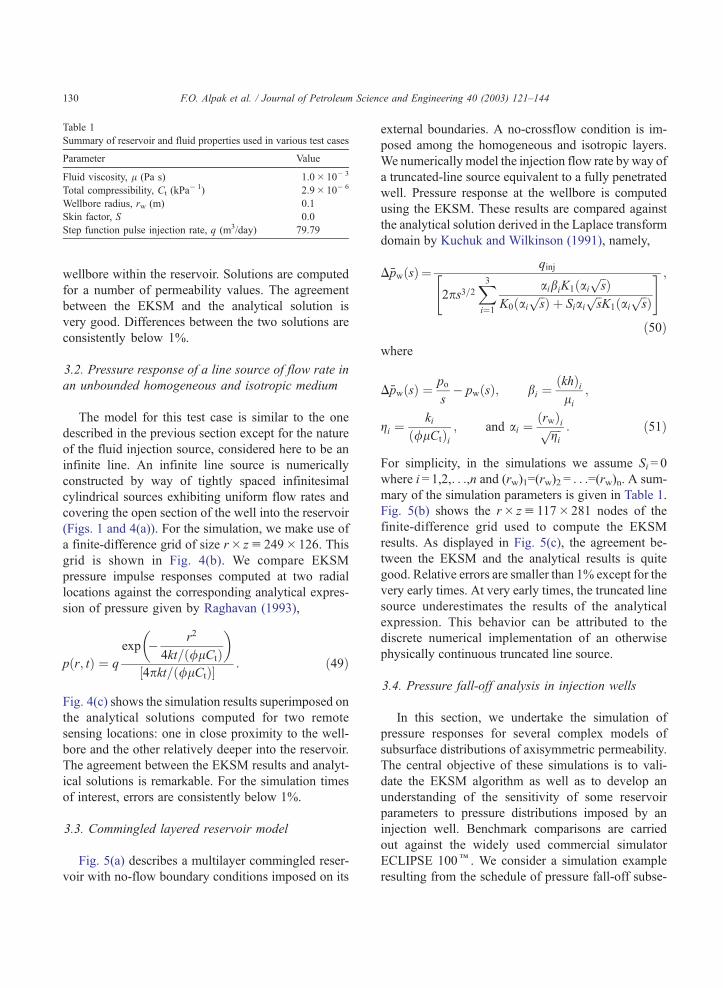
Table 1

Summary of reservoir and fluid properties used in various test cases

Parameter Value

Fluid viscosity, l (Pa s) 1.0� 10� 3

Total compressibility, Ct (kPa� 1) 2.9� 10� 6

Wellbore radius, rw (m) 0.1

Skin factor, S 0.0

Step function pulse injection rate, q (m3/day) 79.79


wellbore within the reservoir. Solutions are computed

for a number of permeability values. The agreement

between the EKSM and the analytical solution is

very good. Differences between the two solutions are

consistently below 1%.

3.2. Pressure response of a line source of flow rate in

an unbounded homogeneous and isotropic medium

The model for this test case is similar to the one

described in the previous section except for the nature

of the fluid injection source, considered here to be an

infinite line. An infinite line source is numerically

constructed by way of tightly spaced infinitesimal

cylindrical sources exhibiting uniform flow rates and

covering the open section of the well into the reservoir

(Figs. 1 and 4(a)). For the simulation, we make use of

a finite-difference grid of size r� zu 249� 126. This

grid is shown in Fig. 4(b). We compare EKSM

pressure impulse responses computed at two radial

locations against the corresponding analytical expres-

sion of pressure given by Raghavan (1993),

pðr; tÞ ¼ q

exp � r2

4kt=ð/lCtÞ

� �½4pkt=ð/lCtÞ�

: ð49Þ

Fig. 4(c) shows the simulation results superimposed on

the analytical solutions computed for two remote

sensing locations: one in close proximity to the well-

bore and the other relatively deeper into the reservoir.

The agreement between the EKSM results and analyt-

ical solutions is remarkable. For the simulation times

of interest, errors are consistently below 1%.

3.3. Commingled layered reservoir model

Fig. 5(a) describes a multilayer commingled reser-

voir with no-flow boundary conditions imposed on its

external boundaries. A no-crossflow condition is im-

posed among the homogeneous and isotropic layers.

We numerically model the injection flow rate by way of

a truncated-line source equivalent to a fully penetrated

well. Pressure response at the wellbore is computed

using the EKSM. These results are compared against

the analytical solution derived in the Laplace transform

domain by Kuchuk and Wilkinson (1991), namely,

DpwðsÞ ¼qinj

2ps3=2X3i¼1

aibiK1ðaiffiffis

p ÞK0ðai

ffiffis

p Þ þ Siaiffiffis

pK1ðai

ffiffis

p Þ

" # ;

ð50Þwhere

DpwðsÞ ¼po

s� pwðsÞ; bi ¼

ðkhÞili

;

gi ¼ki

ð/lCtÞi; and ai ¼

ðrwÞiffiffiffiffigi

p : ð51Þ

For simplicity, in the simulations we assume Si = 0

where i = 1,2,. . .,n and (rw)1=(rw)2 = . . .=(rw)n. A sum-

mary of the simulation parameters is given in Table 1.

Fig. 5(b) shows the r� zu 117� 281 nodes of the

finite-difference grid used to compute the EKSM

results. As displayed in Fig. 5(c), the agreement be-

tween the EKSM and the analytical results is quite

good. Relative errors are smaller than 1% except for the

very early times. At very early times, the truncated line

source underestimates the results of the analytical

expression. This behavior can be attributed to the

discrete numerical implementation of an otherwise

physically continuous truncated line source.

3.4. Pressure fall-off analysis in injection wells

In this section, we undertake the simulation of

pressure responses for several complex models of

subsurface distributions of axisymmetric permeability.

The central objective of these simulations is to vali-

date the EKSM algorithm as well as to develop an

understanding of the sensitivity of some reservoir

parameters to pressure distributions imposed by an

injection well. Benchmark comparisons are carried

out against the widely used commercial simulator

ECLIPSE 100k. We consider a simulation example

resulting from the schedule of pressure fall-off subse-

Fig. 4. Homogeneous and isotropic reservoir model constructed to simulate the pressure response of a long line source of flow rate in an

unbounded permeable medium. (a) Description of the reservoir model. The associated reservoir and fluid properties are listed in Table 1. (b)

Vertical cross-section of the 249� 126 finite-difference simulation grid. (c) Comparison of numerical (EKSM) and analytical pressure impulse

solutions in the time domain. Solutions are computed at a point vertically centered within the reservoir and in close proximity to the well

boundary (r = 0.1 m) and at a second point at r = 1.02 m.


quent to a 135-hour-long constant downhole injection

rate of 79.79 m3/day (step-function excitation). Fluid

injection is modeled using a truncated line source

representing the response of a fully penetrated well

across the formation of interest. The simulations are

presented as time-domain pressure responses sampled

in logarithmic time during a 100-hour-long shut-in

interval subsequent to a constant rate injection pulse.

We make use of the same r� zu 117� 281 simula-

tion grid illustrated in Fig. 5(b) and of the same

reservoir and fluid properties detailed in Table 1.

3.4.1. Homogeneous and isotropic reservoir model

Fig. 6(a) shows the example of a homogenous and

isotropic reservoir model. We compute the fall-off

pressure change as a function of time at a point

Fig. 5. Three-layer commingled reservoir model. (a) Description of the reservoir model. The associated reservoir and fluid properties are listed

in Table 1. No-flow condition is imposed to the top and bottom boundaries of the zone of interest. Each layer is homogeneous and isotropic. A

no-crossflow condition is enforced among the layers. The injection flow rate is modeled by way of a truncated-line source equivalent to a fully

penetrated well. (b) Vertical cross-section of the 117� 281 finite-difference simulation grid. (c) Comparison of numerical (EKSM) and

analytical wellbore pressure solutions in the Laplace transform domain.


vertically centered within the reservoir and in very

close proximity to the wellbore. Pressure fall-off

responses calculated with the EKSM algorithm for

various permeability values are in excellent agreement

with ECLIPSE 100k simulations. Results of this

simulation exercise are summarized in Fig. 6(b). As

expected, fast declining pressure fall-off responses are

observed for increasingly large values of permeability.

Relative errors between the EKSM and the ECLIPSE

100k results are less than 1%.

A more practical version of the model described

above is the one that includes variations of permeabil-

ity in response to water and oil saturations (relative

permeability). Such a model is illustrated in Fig. 7(a).

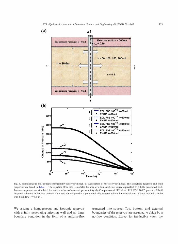
Fig. 6. Homogeneous and isotropic permeability reservoir model. (a) Description of the reservoir model. The associated reservoir and fluid

properties are listed in Table 1. The injection flow rate is modeled by way of a truncated-line source equivalent to a fully penetrated well.

Pressure responses are simulated for various values of reservoir permeability. (b) Comparison of EKSM and ECLIPSE 100k pressure fall-off

response solutions in the time domain. Solutions are computed at a point vertically centered within the reservoir and in close proximity to the

well boundary (r = 0.1 m).


We assume a homogeneous and isotropic reservoir

with a fully penetrating injection well and an inner

boundary condition in the form of a uniform-flux

truncated line source. Top, bottom, and external

boundaries of the reservoir are assumed to abide by a

no-flow condition. Except for irreducible water, the

Fig. 7. Composite water–oil bank reservoir model. (a) Description of the reservoir model. The associated reservoir and fluid properties are listed

in Table 1. The injection flow rate is modeled by way of a truncated-line source equivalent to a fully penetrated well. Pressure responses are

simulated for various locations of saturation front. (b) Assumed saturation-relative permeability dependence for the medium. The locations and

values of end-point relative permeabilities employed in our simulations are indicated on the relative permeability curves. (c) Comparison of

EKSM and ECLIPSE 100k pressure fall-off response solutions in the time domain. Solutions are computed at a point vertically centered within

the reservoir and in close proximity to the well boundary (r = 0.1 m).


reservoir is assumed to be initially filled with oil of a

small and constant compressibility. Water is injected

into the well at a constant rate, thus displacing oil away

from the wellbore. Although, strictly speaking, the

displacement process should be described by two-

phase continuity equations, we consider a commonly

used simplification that approximates the saturation

profile with a step change (shock saturation front).

This assumption is equivalent to the case of a moving

boundary two-zone composite reservoir model. We

Fig. 8. Reservoir model exhibiting anisotropic permeability. (a) Description of the reservoir model. Formation layers are in pressure

communication. The associated reservoir and fluid properties are listed in Table 1. The injection flow rate is modeled by way of a truncated-line

source equivalent to a fully penetrated well. Pressure responses are simulated for various permeability anisotropy ratios kr/kz. (b) Comparison of

EKSM and ECLIPSE 100k pressure fall-off response solutions in the time-domain. Solutions are computed at a point vertically centered within

the reservoir and in close proximity to the well boundary (r = 0.1 m).



anticipate that the mean fluid properties of the invaded

zone would roughly correspond to values at residual

oil saturation. Presumably, fluid properties of the

formation ahead of the saturation discontinuity, re-

ferred to as uninvaded zone, are determined by the

properties of the in situ oil. The idealized moving

boundary (or the water front) in the current context is

expected to approximately coincide with the Buckley–

Fig. 9. Three-layer reservoir model. (a) Description of the reservoir mode

reservoir and fluid properties are listed in Table 1. The injection flow rate

penetrated well. (b) Comparison of EKSM and ECLIPSE 100k pressure fa

at points vertically centered within each layer and in close radial proximi

EKSM and ECLIPSE 100k at a second set of locations relatively furthe

Leverett discontinuity (Buckley and Leverett, 1941),

or more precisely, the capillary transition region. A

slow-moving boundary is assumed. We describe the

permeability field by computing effective single-phase

permeabilities for the invaded (water) and uninvaded

(oil) zones. Fig. 7(a) shows the composite reservoir

model constructed following these assumptions. Ef-

fective single-phase permeabilities are computed using

l. Formation layers are in pressure communication. The associated

is modeled by way of a truncated-line source equivalent to a fully

ll-off response solutions in the time domain. Solutions are computed

ty to the well boundary (r = 0.1 m). (c) Comparison of solutions of

r in the reservoir (r = 1.05 m).


end-point relative permeability values for a water-wet

medium. The assumed saturation-relative permeability

dependence for the medium is shown in Fig. 7(b). We

use only the end-point relative permeability values

shown in that figure. Simulations of fall-off pressure

response are performed for various locations of the

Fig. 10. Three-layer, nine-block reservoir model. (a) Description of the res

associated reservoir and fluid properties are listed in Table 1. The injection f

fully penetrated well. (b) Comparison of EKSM and ECLIPSE 100k pr

computed at points vertically centered within each layer and in close rad

solutions of EKSM and ECLIPSE 100k at a second set of locations rela

water front (parameter rbank). A slow moving bound-

ary assumption is imposed, i.e., we assume that the

location of the fluid boundary remains stationary

during the course of the pressure transient test. Fig.

7(c) shows the comparison of simulation results

obtained with both EKSM and ECLIPSE 100k for

ervoir model. Formation layers are in pressure communication. The

low rate is modeled by way of a truncated-line source equivalent to a

essure fall-off response solutions in the time-domain. Solutions are

ial proximity to the well boundary (r = 0.1 m). (c) Comparison of

tively further in the reservoir (r = 1.05 m).

Table 2

Comparison of computation times associated with various test cases

Machine:

SGI Octane

(300 MHz)

ECLIPSE 100k (A) EKSM (B) Ratio of the

CPU times

(A)/(B)

Grid r� zu 105� 200 r� zu 105� 203 –

CPU time (s) 12.71 5.38 2.36

Grid r� zu 125� 200 r� zu 125� 203 –

CPU time (s) 15.00 8.13 1.85

Grid r� zu 117� 281 r� zu 117� 281 –

CPU time (s) 20.68 11.56 1.79

Computational complexity is varied by changing the spatial

discretization of the one-layer one-block reservoir model shown in

Fig. 6(a).


the same pressure sampling location described in the

previous case. In general, there is a good agreement

between both results. Relative errors are within 1–4%

for various locations of the saturation front. Compar-

ison of the simulation results for homogeneous and

composite reservoir models suggests that the pressure

response is sensitive to both the single-phase perme-

ability field and the location of the water front.

3.4.2. Reservoir model exhibiting anisotropic

permeability

Vertical and horizontal permeabilities are com-

monly not equivalent in practical subsurface reser-

voir models. The ratio of the horizontal permeability,

kr, to the vertical permeability, kz, is referred to as

the anisotropy ratio, kr/kz. The EKSM algorithm

developed in this paper can be used for the simula-

tion of pressure responses of anisotropic reservoirs

describable with a 2D axisymmetric coordinate

frame. Fig. 8(a) shows an example of an anisotropic

reservoir model. Pressure responses due to this

reservoir are computed with both the EKSM and

ECLIPSE 100k simulators assuming an observation

point vertically centered in the reservoir and in close

Table 3

Comparison of computation times associated with various test cases

Machine: SGI Octane (300 MHz) ECLIPSE 100k (A)

Grid r� zu 200� 200

CPU time (s) [one-layer one-block

reservoir; Fig. 6(a)]

31.00

CPU time (s) [three-layer nine-block

reservoir; Fig. 10(a)]

33.95

Simulation results from both simulators agree within 1% of each other fo

proximity to the wellbore. Simulation results are

displayed in Fig. 8(b) for various anisotropy ratios

ranging from 1 to 30. The EKSM and ECLIPSE

100k results agree within 1–4% of each other for

the various simulation examples.

3.4.3. Two-dimensional multilayer and multiblock

reservoir models

We simulate fall-off pressure changes in the pres-

ence of both a simple 2D three-layer model and a

relatively more complex three-layer, nine-block reser-

voir model. Fig. 9(a) illustrates the three-layer reser-

voir model and its associated rock properties. In both

cases, pressure observation points are vertically cen-

tered within the layers at two different radial locations.

Fig. 9(b) shows the pressure changes simulated for the

three-layer reservoir model at a point located in close

proximity to the wellbore (r = 0.1 m) at three vertical

observation locations within the permeable medium.

Pressure changes are computed with both the EKSM

algorithm and ECLIPSE 100k, and are displayed as

superimposed time domain variations. A similar plot is

shown in Fig. 9(c) that describes modeling results for a

deeper radial location (r = 1.05 m) within three layer-

mid-depths. A percent error analysis indicates an

agreement within 1% for both simulations.

Fig. 10(a) describes the three-layer, nine-block

reservoir model and its associated rock properties.

Pressure observation locations are the same as in the

previous case. Results of this simulation exercise are

shown in Fig. 10(b) in the form of time-domain

pressure change at a location within the permeable

medium in close proximity to the wellbore (r= 0.1 m).

Fig. 10(c), on the other hand, describes results

obtained for a deeper radial location (r = 1.05 m)

within all three layer-mid-depths. The EKSM and

ECLIPSE 100k numerical simulations agree within

1% of each other.

EKSM (B) Ratio of the CPU times (A)/(B)

r� zu 117� 281 –

11.56 2.68

11.66 2.91

r the test problems reported in this table.


We also perform benchmark simulations of

ECLIPSE 100k and EKSM to assess computational

efficiency. Results of our benchmark study are pre-

sented in Tables 2 and 3. All the simulations are

performed on a SGI Octane 300 MHz computer.

Comparison of simulation times indicates that EKSM

provides approximately a one-and-a-half- to three-fold

improvement in performance with respect to the com-

mercial simulator for the test examples shown in

Tables 2 and 3. Moreover, our benchmark studies

suggest that the EKSM algorithm is suitable for

solving large-scale inverse problems of single-phase

fluid flow phenomena.

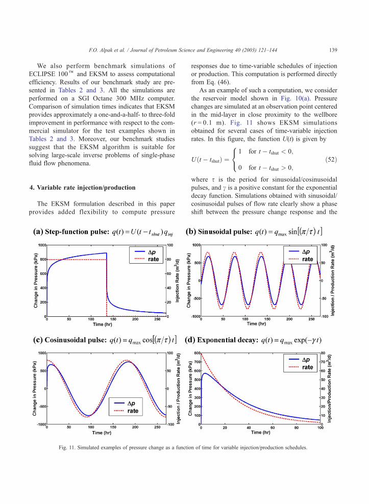
4. Variable rate injection/production

The EKSM formulation described in this paper

provides added flexibility to compute pressure

Fig. 11. Simulated examples of pressure change as a functio

responses due to time-variable schedules of injection

or production. This computation is performed directly

from Eq. (46).

As an example of such a computation, we consider

the reservoir model shown in Fig. 10(a). Pressure

changes are simulated at an observation point centered

in the mid-layer in close proximity to the wellbore

(r = 0.1 m). Fig. 11 shows EKSM simulations

obtained for several cases of time-variable injection

rates. In this figure, the function U(t) is given by

Uðt � tshutÞ ¼1 for t � tshut < 0;

0 for t � tshut > 0;

8<: ð52Þ

where s is the period for sinusoidal/cosinusoidal

pulses, and c is a positive constant for the exponential

decay function. Simulations obtained with sinusoidal/

cosinusoidal pulses of flow rate clearly show a phase

shift between the pressure change response and the

n of time for variable injection/production schedules.

Fig. 12. Pressure derivative and injection rate behavior during (a) build-up and (b) fall-off time intervals for the step-function excitation, and

during (c) pulsation of the sinusoidal excitation.



pulsing rate function. Consistent with the physics of a

slightly compressible fluid and pressure wave propa-

gation, the pressure response exhibits a phase shift

with respect to the excitation pulse by a constant

amount. This phase shift increases with increasing

values of compressibility, Ct.

Finally, the EKSM algorithm provides a simple and

direct way to compute the pressure derivative with

respect to time. From Eq. (46), one can write

Bp

Bt¼ B

Bt

"Z t

�lqsf ðsÞ½Gðr; z; t�sÞþdðt�sÞDpskin�ds

#:

ð53Þ

Fig. 12 shows examples of the computation of pres-

sure derivatives associated with the injection/produc-

tion schedules described in Fig. 11(a) and (b). Fig.

12(a) shows the pressure derivative and the injection

rate as functions of time computed for the build-up

time interval. Fig. 12(b), on the other hand, displays

pressure derivative behavior during the shut-in period

resulting from the enforcement of step-function pulse

excitation. Pressure derivative and pulsing rate behav-

ior simulated for the sinusoidal pulse excitation dis-

played in Fig. 11(b) are shown in Fig. 12(c).

Pressure and pressure derivative responses of mul-

tirate tests can be readily evaluated with the formula-

Fig. 13. Simulated example of (a) pressure change and (b) pressure derivati

The actual injection schedule is approximated by a series of consecutive

tions shown in Eqs. (46) and (53). Consequently,

pressure test schedules with arbitrarily varying flow

rates can be simulated via EKSM when the flow rate

function can be approximated with a series of step-

functions. An example simulation of an injection test

is shown in Fig. 13(a) and (b). Both actual and

approximate flow rate schedules are superimposed

on the pressure and the pressure derivative plots

displayed in Fig. 13(a) and (b), respectively.

5. Summary and conclusions

An important feature of the EKSM developed in

this paper is its ability to provide pressure solutions in

response to axisymmetric single-phase flow for a

multitude of times with practically the same efficiency

as that of a single time solution. Moreover, the EKSM

formulation can be easily adapted to provide solutions

of pressure in the Laplace transform domain without

appreciable computer overhead. The same formula-

tion requires only a minor modification to yield

solutions of the time derivative of pressure. In addi-

tion, the EKSM formulation is also readily applicable

for the simulation of variable flow rate schedules. In

this paper, we considered pressure change and pres-

sure derivative responses for simple variable rate test

schedules.

ve as a function of time for an arbitrarily varying injection schedule.

step-functions.


The high efficiency of the EKSM algorithm is

primarily due to the usage of inverse powers of the

finite-difference operator, A, when computing the

pressure solution. Extensive tests have shown that

the simultaneous use of inverse and positive powers

ofA provides a significant acceleration in convergence

compared to a conventional implementation of Lanc-

zos recurrence. This property of the EKSM algorithm

yields approximately one-and-a-half- to three-fold

improvement in performance with respect to that of

the commercial software used for comparisons. Sen-

sitivity studies carried out to assess the influence of

specific petrophysical parameters on pressure meas-

urements also suggest that the EKSM algorithm pos-

sesses the degree of efficiency necessary to approach

practical inverse problems. Comparisons of EKSM

numerical simulation results with respect to those

obtained using analytical solutions for point and line

sources validate the accuracy of the developed numer-

ical solver. These benchmark tests indicate that EKSM

results and analytical solutions agree within 1% of

each other. The accuracy of the EKSM algorithm is

also assessed for various geometrically complex res-

ervoir models by comparing EKSM simulations

against numerical solutions computed using a com-

mercial reservoir simulator, ECLIPSE 100k. Pressure

responses from both simulators agree within 1–4% of

each other.

Nomenclature

A square symmetric nonnegative matrix resul-

ting from the finite-difference spatial discre-

tization of the operator A[u]

A functional operator

a diagonal elements of the tridiagonal matrix T

given by Eq. (33)

B inverse of matrix A

b off-diagonal elements of the three-diagonal

matrix T given by Eq. (33)

b0 vector used in the simplified formulation of

matrix D given by Eq. (34)

c set of coefficients used in Eq. (39)

CG conjugate gradient

CPU central processing unit

Ct total compressibility

D rank 1 matrix used in the augmented for-

mulation of Ritz matrix R

EKSM extended Krylov subspace method

ei unit vector of order i

G full matrix given by Eq. (32)

G Green’s function

Gw Green’s function at the open section of the

wellbore boundary

G1 asymptotic solution of the Green’s function

as t! 0

H tridiagonal symmetric Ritz matrix given by

Eq. (37)

H Heaviside’s step function

h formation thickness

I identity matrix

k second-order permeability tensor

k single-phase permeability, integer used in

describing matrix–vector sizes

kr relative permeability for a particular phase

koro end-point relative permeability for oleic phase

korw end-point relative permeability for aqueous

phase

kro relative permeability for oleic phase

krw relative permeability for aqueous phase

K0 modified Bessel function of second kind,

zeroth order

K1 modified Bessel function of second kind,

first order

L total number of elements in matrix A

l1 lower bound of the wellbore open interval

l2 upper bound of the wellbore open interval

M number of grid points in the vertical direction

m integer used in describing matrix–vector

sizes

N number of grid points in the radial direction

n integer used in describingmatrix–vector sizes

p pressure

PDE partial differential equation

po initial formation pressure

pw pressure at the wellbore

Q orthogonal matrix made up of Lanczos

vectors given by Eq. (38)

q injection/production rate, Lanczos vectors

qinj injection rate

qmax amplitude of sinusoidal and cosinusoidal

flow rate pulses, starting value of the

exponentially decaying flow rate function

qsf flow rate on the open section of the well

R Ritz matrix shown in Eq. (30) and given by

Eq. (31)

r space vector


r radial spatial coordinate, radial coordinate

indicator in the cylindrical coordinate sys-

tem, vector given by Eq. (38)

re reservoir external radius

rw wellbore radius

rbank radial distance between water and oil bank

interface from the wellbore

S skin factor, phase saturation

s Laplace image space variable

Sor residual oleic phase saturation

Sw aqueous phase saturation

Swirr irreducible aqueous phase saturation

SLDM spectral Lanczos decomposition method

T mobility tensor

T tridiagonal matrix given by Eq. (33)

T mobility

t time

tshut time at which the well is shut in

U Laplace transform of Green’s function, the

function defined by Eq. (52)

u vector notation for the variable u given by

Eq. (23)

u variable that results from the substitution

given by Eq. (23)

u spatial continuation of u described by Eq. (21)

v fluid velocity vector

v set of vectors employed in the three-term

Gram–Schmidt recurrence [Eq. (45)]

W orthogonal matrix described in the context of

Eq. (30)

x coordinate indicator in the Cartesian coor-

dinate system

y coordinate indicator in the Cartesian coor-

dinate system

z coordinate indicator in the Cartesian coor-

dinate system, vertical spatial coordinate,

vertical coordinate indicator in the cylindri-

cal coordinate system

Greek symbols

a diagonal elements of the tridiagonal matrix

H, substitution variable that appears in Eq.

(50) and defined in Eq. (51)

b off-diagonal elements of the tridiagonal

matrix H, substitution variable that appears

in Eq. (50) and defined in Eq. (51)

Dpw change in the pressure response at the

wellbore given by Eq. (50)

Dpskin pressure drop due to the presence of the skin

factor

DS saturation jump

d Dirac delta function

BX closed boundary of the domain XBX1 part of the closed boundary of the domain X

that corresponds to the open section of the

wellbore

BX1 boundary of the fictitious outer domain X1

BX2 part of the closed boundary of the domain Xthat corresponds to the no-flow section of the

wellbore and sealing upper, lower, and outer

boundaries

BX2 boundary of the fictitious outer domain X2

/ porosity

c positive constant for the exponential-decay

flow rate function

g substitution variable that appears in Eq.

(50) and defined in Eq. (51) [pressure

diffusivity]

j extended Krylov subspace

l fluid viscosity

q mass density of the fluid

s vector notation for the initial condition

variable r given by Eq. (26)

r initial condition variable that results from the

substitution given by Eq. (26)

s variable of integration in Eqs. (46) and (53),

period for sinusoidal and cosinusoidal flow

rate pulses

X spatial domain in which the PDE describing

the pressure diffusion problem [Eq. (3)] is

solved subject to appropriate boundary con-

ditions [permeable medium], variable of inte-

gration in Eq. (20)

X entire spatial domain of the problem includ-

ing the fictitious outer domains

X1 fictitious outer domain across the surface of

the permeable medium that is open to flow

[open interval of the wellbore]

X2 fictitious outer domain across the no-flow

boundaries of the permeable medium [closed

interval of the wellbore, sealing upper and

lower layers, and formations beyond the no-

flow external boundary of the permeable

medium]

x variable of integration in Eqs. (5), (11), and

(15)


Subscripts

i integer count index

k the number of the inverse powers of the

discrete finite-difference operator A used in

constructing the extended Krylov subspace j[Eq. (30)], matrix–vector size index

m the number of the positive powers of the


constructing the extended Krylov subspace j[Eq. (30)], matrix–vector size index

r entity in the radial direction

z entity in the vertical direction

h entity in the azimuthal direction

Superscripts

(i) integer count index

k the number of the inverse powers of the


constructing the extended Krylov subspace j(k) vector size index

m the number of the positive powers of the


constructing the extended Krylov subspace jT transpose

Acknowledgements

We would like to express our deepest appreciation

to Baker Atlas, Halliburton, and Schlumberger for

funding of this work through UT Austin’s Center of

Excellence in Formation Evaluation. A note of gra-

titude goes to Vladimir Druskin for his technical

advice during the earlier phases of the work reported

in this paper.

References

Allers, A., Sezginer, A., Druskin, V., 1994. Solution of 2.5-dimen-

sional problems using the Lanczos decomposition. Radio Sci. 29

(4), 955–963.

Alpak, F.O., Torres-Verdın, C., Sepehrnoori, K., Fang, S., 2002.

Numerical sensitivity studies for the joint inversion of pressure

and DC resistivity measurements acquired with in-situ perma-

nent sensors. Paper SPE 77621 presented at the SPE Annual

Technical Conference and Exhibition, San Antonio, TX, 29

September–2 October.

Aziz, K., Settari, A., 1979. Petroleum Reservoir Simulation. Ap-

plied Science Publishers, New York.

Buckley, S.E., Leverett, M.C., 1941. Mechanism of fluid displace-

ment in sands. J. Pet., 107–116.

Druskin, V., Knizhnerman, L., 1988. A spectral semi-discrete meth-

od for the numerical solution of 3-D non-stationary problems in

electrical prospecting. Izv. Acad. Sci. USSR Phys. Solid Earth

24, 63–74.

Druskin, V., Knizhnerman, L., 1989. Two polynomial methods to

compute functions of symmetric matrices. Comput. Maths.

Math. Phys. 29, 112–121.

Druskin, V., Knizhnerman, L., 1991. Error bounds in the simple

Lanczos procedure when computing functions of symmetric

matrices and eigenvalues. J. Comput. Math. Phys. 31, 20–30.

Druskin, V., Knizhnerman, L., 1994a. On application of the Lanc-

zos method to solution of some partial differential equations.

J. Comput. Appl. Math. 50, 255–262.

Druskin, V., Knizhnerman, L., 1994b. Spectral approach to solving

three-dimensional Maxwell’s diffusion equations in the time and

frequency domains. Radio Sci. 29 (4), 937–953.

Druskin, V., Knizhnerman, L., 1998. Extended Krylov subspaces:

approximation of the matrix square root and related functions.

SIAM J. Matrix Anal. Appl. 19, 755–771.

Dunbar, W.S., Woodbury, A.D., 1989. Application of the Lanczos

algorithm to the solution of the groundwater flow equation.

Water Resour. Res. 25, 551–558.

Knizhnerman, L., Druskin, V., Liu, Q.-H., Kuchuk, F.J., 1994.

Spectral Lanczos decomposition method for solving single-

phase fluid flow in porous media. Numer. Methods Partial Dif-

fer. Equ. 10, 569–580.

Kuchuk, F.J., Wilkinson, D.J., 1991. Transient pressure behav-

ior of commingled reservoirs. Soc. Pet. Eng. Form. Eval.,

111–120.

Lanczos, C., 1950. An iteration method for the solution of the

eigenvalue problem of linear differential and integral operators.

J. Res. Natl. Bur. Stand. 45, 255–282.

Muskat, M., 1937. The Flow of Homogeneous Fluids Through

Porous Media. McGraw-Hill, New York.

Nour-Omid, B., 1987. Lanczos method for heat conduction analy-

sis. Int. J. Numer. Methods Eng. 24, 251–262.

Nour-Omid, B., Clough, R.W., 1984. Dynamic analysis of structure

using Lanczos co-ordinates. Earthquake Eng. Struct. Dyn. 12,

565–577.

Paige, C.C., Sounders, M.A., 1975. Solution of sparse indefinite

systems of linear equations. SIAM J. Numer. Anal. 12, 617–629.

Parlett, B.N., 1980a. The Symmetric Eigenvalue Problem. Prentice-

Hall, Englewood Cliffs, NJ.

Parlett, B.N., 1980b. A new look at the Lanczos algorithm for

solving symmetric systems of linear equations. Linear Algebra

Appl. 29, 323–346.

Peaceman, D.W., 1977. Fundamentals of Numerical Reservoir Sim-

ulation. Elsevier, New York.

Raghavan, R., 1993. Well Test Analysis. Prentice-Hall, Englewood

Cliffs, NJ.

van der Vorst, H.A., 1987. An iterative solution method for solving

f (A)x = b using Krylov subspace information obtained for the

symmetric positive definite matrix A. J. Comput. Appl. Math.

18, 249–263.

An extended Krylov subspace method to simulate single ... · An extended Krylov subspace method to...

Documents

Transcript of An extended Krylov subspace method to simulate single ... · An extended Krylov subspace method to...