An Experimental Study of Dynamic Dominators∗

Loukas Georgiadis1 Giuseppe F. Italiano2 Luigi Laura3 Federico Santaroni2

April 12, 2016

Abstract

Motivated by recent applications of dominator computations, we consider the problem ofdynamically maintaining the dominators of flow graphs through a sequence of insertions anddeletions of edges. Our main theoretical contribution is a simple incremental algorithm thatmaintains the dominator tree of a flow graph with n vertices through a sequence of k edge in-sertions in O(mminn, k+ kn) time, where m is the total number of edges after all insertions.Moreover, we can test in constant time if a vertex u dominates a vertex v, for any pair of queryvertices u and v. Next, we present a new decremental algorithm to update a dominator treethrough a sequence of edge deletions. Although our new decremental algorithm is not asymp-totically faster than repeated applications of a static algorithm, i.e., it runs in O(mk) time for kedge deletions, it performs well in practice. By combining our new incremental and decremen-tal algorithms we obtain a fully dynamic algorithm that maintains the dominator tree throughintermixed sequence of insertions and deletions of edges. Finally, we present efficient imple-mentations of our new algorithms as well as of existing algorithms, and conduct an extensiveexperimental study on real-world graphs taken from a variety of application areas.

1 Introduction

A flow graph G = (V,E, s) is a directed graph with a distinguished start vertex s ∈ V . A vertex v isreachable in G if there is a path from s to v; v is unreachable if no such path exists. The dominatorrelation on G is defined for the set of reachable vertices as follows. A vertex w dominates a vertexv if every path from s to v includes w. We let Dom(v) denote the set of all vertices that dominatev. If v is reachable then Dom(v) ⊇ s, v; otherwise Dom(v) = ∅. For a reachable vertex v, s andv are its trivial dominators. A vertex w ∈ Dom(v)− v is a proper dominator of v. The immediatedominator of a vertex v 6= s, denoted d(v), is the unique vertex w 6= v that dominates v and isdominated by all vertices in Dom(v) − v. The dominator relation is reflexive and transitive. Itstransitive reduction is a rooted tree, the dominator tree D: u dominates w if and only if u is anancestor of w in D. To form D, we make each reachable vertex v 6= s a child of its immediatedominator.

The problem of finding dominators has been extensively studied, as it occurs in several appli-cations. The dominator tree is a central tool in program optimization and code generation [12].

1Department of Computer Science & Engineering, University of Ioannina, Greece. E-mail: loukas@cs.uoi.gr.2Dipartimento di Ingegneria Civile e Ingegneria Informatica, Universita di Roma “Tor Vergata”, Roma, Italy.

E-mail: giuseppe.italiano@uniroma2.it, santaroni@uniroma2.it.3Dipartimento di Ingegneria Informatica, Automatica e Gestionale e Centro di Ricerca per il Trasporto e la

Logistica (CTL), “Sapienza” Universita di Roma, Roma, Italy. E-mail: laura@dis.uniroma1.it.∗A preliminary version of this paper appeared in the Proceedings of the 20th Annual European Symposium on

Algorithms, pages 491–502, 2012.

1

arX

iv:1

604.

0271

1v1

[cs

.DS]

10

Apr

201

6

Dominators have also been used in constraint programming [38], circuit testing [5], theoretical bi-ology [2], memory profiling [35], fault-tolerant computing [6], connectivity and path-determinationproblems [18, 19, 20, 21, 29, 30, 31, 32], and the analysis of diffusion networks [27]. Allen andCocke showed that the dominator relation can be computed iteratively from a set of data-flowequations [1]. A direct implementation of this method has an O(mn2) worst-case time bound, fora flow graph with n vertices and m edges. Cooper et al. [11] presented a clever tree-based space-efficient implementation of the iterative algorithm. Although it does not improve the O(mn2)worst-case time bound, the tree-based version is much more efficient in practice. Purdom andMoore [37] gave an algorithm, based on reachability, with complexity O(mn). Improving on previ-ous work by Tarjan [44], Lengauer and Tarjan [33] proposed an O(m log(m/n+1) n)-time algorithmand a more complicated O(mα(m,n))-time version, where α(m,n) is an extremely slow-growingfunctional inverse of the Ackermann function [46]. Subsequently, more-complicated but truly linear-time algorithms to compute D were discovered [3, 7, 8, 24], as well as near-linear-time algorithmsthat use simple data structures [16, 17].

An experimental study of static algorithms for computing dominators was presented in [26],where careful implementations of both versions of the Lengauer-Tarjan algorithm, the iterativealgorithm of Cooper et al., and a new hybrid algorithm (snca) were given. In these experi-mental results the performance of all these algorithms was similar, but the simple version of theLengauer-Tarjan algorithm and the hybrid algorithm were most consistently fast, and their ad-vantage increased as the input graph got bigger or more complicated. The graphs used in [26]were taken from the application areas mentioned above and have moderate size (at most a fewthousand vertices and edges) and simple enough structure that they can be efficiently processedby the iterative algorithm. Recent experimental results for computing dominators in large graphsare reported in [15, 19, 22, 23]. There it is apparent that the simple iterative algorithms are notcompetitive with the more sophisticated algorithms based on Lengauer-Tarjan for larger and morecomplicated graphs.

Here we consider the problem of dynamically maintaining the dominator relation of a flowgraph that undergoes both insertions and deletions of edges. Vertex insertions and deletions canbe simulated using combinations of edge updates. We recall that a dynamic graph problem is saidto be fully dynamic if it requires to process both insertions and deletions of edges, incremental if itrequires to process edge insertions only and decremental if it requires to process edge deletions only.The fully dynamic dominators problem arises in various applications, such as data flow analysisand compilation [10]. Moreover, [18, 30] imply that a fully dynamic dominators algorithm can beused for dynamically testing 2-vertex connectivity, and maintaining the strong articulation pointsof a digraph. The decremental dominators problem appears in the computation of 2-connectedcomponents in digraphs [34, 29, 32].

The problem of updating the dominator relation has been studied for few decades (see, e.g., [4, 9,10, 36, 39, 42]). However, a worst-case complexity bound for a single update better than O(m) hasbeen only achieved for special cases, mainly for incremental or decremental problems. Specifically,the algorithm of Cicerone et al. [10] achieves O(nmaxk,m0 + q) running time for processinga sequence of k edge insertions interspersed with q queries of the type “does u dominate v?”,for a flow graph with n vertices and initially m0 edges. This algorithm, however, requires O(n2)space, as it needs to maintain the transitive closure of the graph. The same bounds are alsoachieved for a sequence of k deletions, but only for a reducible flow graph (defined below). Alstrupand Lauridsen describe in a technical report [4] an algorithm that maintains the dominator treethrough a sequence of k edge insertions interspersed with q queries in O(mmink, n + q) time.In this bound m is the number of edges after all insertions. Unfortunately, the description andthe analysis of this algorithm are incomplete. Our main theoretical contribution is to provide

2

a simple incremental algorithm that maintains the dominator tree through a sequence of k edgeinsertions in O(mmink, n+ kn) time. We can also answer dominance queries (test if a vertex udominates another vertex v) in constant time. Moreover, we provide an efficient implementation ofthis algorithm that performs very well in practice.

Although theoretically efficient solutions to the fully dynamic dominators problem appear stillbeyond reach, there is a need for practical algorithms and fast implementations in several applica-tion areas. In this paper, we also present new fully dynamic dominators algorithms and efficientimplementations of known algorithms, such as the algorithm by Sreedhar, Gao and Lee [42]. Weevaluate the implemented algorithms experimentally using real data taken from the applicationareas of dominators. To the best of our knowledge, the only previous experimental study of (fully)dynamic dominators algorithms appears in [36]; here we provide new algorithms, improved im-plementations, and an experimental evaluation using bigger graphs taken from a larger variety ofapplications. Other previous experimental results, reported in [40] and the references therein, arelimited to comparing incremental algorithms against the static computation of dominators.

2 Basic definitions and properties

The algorithms we consider can be stated in terms of two structural properties of dominator treesthat we discuss next. Let G = (V,E, s) be a flow graph, and let T be a tree rooted at s, withvertex set consisting of the vertices that are reachable from s. For a reachable vertex v 6= s, lett(v) denote the parent of v in T . Tree T has the parent property if for all (v, w) ∈ E such that vis reachable, v is a descendant of t(w) in T . If T has the parent property then t(v) dominates vfor every reachable vertex v 6= s [25]. The next lemma states another useful property of trees thatsatisfy the parent property.

Lemma 2.1. [25] Let T we a tree with the parent property. If v is an ancestor of w in T , there isa path from v to w in G, and every vertex on a simple path from v to w in G is a descendant of vbut not a proper descendant of w in T .

Let T be a tree with the parent property, and let v be a reachable vertex of G. We definethe support spT (v, w) of an edge (v, w) with respect to T as follows: if v = t(w), spT (v, w) = v;otherwise, spT (v, w) is the child of t(w) that is an ancestor of v.

Tree T has the sibling property if v does not dominate w for all siblings v and w. The parentand sibling properties are necessary and sufficient for a tree to be the dominator tree.

Theorem 2.2. [25] Tree T is the dominator tree (T = D) if and only if it has the parent and thesibling properties.

Now consider the effect that a single edge update (insertion or deletion) has on the dominatortree D. Let (x, y) be the inserted or deleted edge. We let G′ and D′ denote the flow graph and itsdominator tree after the update. Similarly, for any function f on V , we let f ′ be the function afterthe update. By definition, D′ 6= D only if x is reachable before the update. We say that a vertexv is affected by the update if d′(v) 6= d(v). (Note that we can have Dom ′(v) 6= Dom(v) even if v isnot affected.) If v is affected then d(v) does not dominate v in G′. This implies that the insertionof (x, y) creates a path from s to v that avoids d(v).

The difficulty in updating the dominance relation lies on two facts: (i) An affected vertex canbe arbitrarily far from the updated edge, and (ii) a single update may affect many vertices. Twopathological examples are shown in Figures 1 and 2. The graph family of Figure 1 contains, forany n ≥ 3, a directed graph with n vertices that consists of the path (s = v0, v1, v2, . . . , vn−1),

3

insert

delete

𝐺

𝑠

𝑣1

𝐷

𝑠

(𝑠 , 𝑣7)

(𝑠 , 𝑣7)

𝐷′

𝐺′

𝑣2

𝑣3

𝑣4

𝑣5

𝑣6

𝑣7

𝑠

𝑣1

𝑣2

𝑣3

𝑣4

𝑣5

𝑣6

𝑣7

𝑠

𝑣1

𝑣2

𝑣3

𝑣4

𝑣5

𝑣6

𝑣7

𝑣1 𝑣2 𝑣3 𝑣4 𝑣5 𝑣6 𝑣7

Figure 1: Pathological updates: Each update (insertion or deletion) affects n− 2 vertices. (In thisinstance n = 8.)

together with the reverse subpath (vn−1, vn−2, . . . , v2). Initially we have d(vi) = vi−1 for all i ∈1, 2, . . . , n − 1. The insertion of edge (s, vn−1) makes d′(vi) = s for all i ∈ 2, 3, . . . , n − 1,while the deletion of (s, vn−1) restores the initial dominator tree. So each single edge updateaffects every vertex except s and v1. A similar example, but for a family of directed acyclicgraphs is shown in Figure 2. This graph family contains, for any n ≥ 3, a directed acyclic graphwith n vertices that consists of the path (s = v0, v1, v2, . . . , vbn/2c−1), together with the edges(vbn/2c−1, vi) for all i ∈ bn/2c, bn/2c + 1, . . . , n − 1. Initially we have d(vi) = vi−1 for all i ∈1, 2, . . . , bn/2c − 1, and d(vi) = vbn/2c−1 for all i ∈ bn/2c, bn/2c + 1, . . . , n − 1. The insertionof edge (s, vn−1) makes d′(vi) = s for all i ∈ bn/2c, bn/2c + 1, . . . , n − 1, while the deletion of(s, vn−1) restores the initial dominator tree. So each single edge update affects dn/2e vertices.Moreover, we can construct sequences of Θ(n) edge insertions (deletions) such that each singleinsertion (deletion) affects Θ(n) vertices. Consider, for instance, the graph family of Figure 1and the sequence of insertions (vn−3, vn−1), (vn−4, vn−1), . . . , (s, vn−1), or the the graph family ofFigure 2 and the sequence of insertions (vbn/2c−2, vn−1), (vbn/2c−3, vn−1), . . . , (s, vn−1). This impliesa lower bound of Ω(n2) time for any algorithm that maintains D (or the complete dominatorrelation) explicitly through a sequence of Ω(n) edge insertions or a sequence of Ω(n) edge deletions,and a lower bound of Ω(mn) time for any algorithm that maintains D (or the complete dominatorrelation) explicitly through an intermixed sequence of Ω(m) edge insertions and deletions, thatholds even for directed acyclic graphs.

Using the structural properties of dominator trees stated above we can limit the number of ver-tices and edges processed during the search for affected vertices. The following fact is an immediateconsequence of the parent and sibling properties of the dominator tree.

Proposition 2.3. An edge insertion can violate the parent property but not the sibling property ofD. An edge deletion can violate the sibling property but not the parent property of D.

Throughout the rest of this paper, (x, y) is the inserted or deleted edge and x is reachable.

4

insert

delete

(𝑠 , 𝑣8)

(𝑠 , 𝑣8)

𝑠

𝑣1

𝑣2

𝑣3

𝑣4

𝑣5 𝑣6 𝑣7 𝑣8 𝑣5 𝑣6 𝑣7 𝑣8 𝑣5 𝑣6 𝑣7 𝑣8

𝑠

𝑣1

𝑣2

𝑣3

𝑣4

𝑠

𝑣1

𝑣2

𝑣3

𝑣4

𝑠

𝑣1

𝑣2

𝑣3

𝑣4

𝑣5 𝑣6 𝑣7 𝑣8

𝐺 𝐷

𝐷′

𝐺′

Figure 2: Pathological updates in the acyclic case: Each update (insertion or deletion) affectsdn/2e vertices. (In this instance n = 9.)

2.1 Edge insertion

We consider two cases, depending on whether y was reachable before the insertion. Suppose firstthat y was reachable. Let ncaD(x, y) be the nearest (lowest) common ancestor of x and y in D. Ifeither ncaD(x, y) = d(y) or ncaD(x, y) = y then, by Theorem 2.2, the inserted edge has no effecton D. Otherwise, the parent property of D implies that ncaD(x, y) is a proper dominator of d(y).In the following, we denote by depth(w) the depth of vertex w in D.

Lemma 2.4. ([39]) Suppose x and y are reachable vertices in G. Let v be a vertex that is affectedafter the insertion of (x, y). Then d′(v) = ncaD(x, y) and d′(v) is a proper ancestor of d(v) in D.

For Lemma 2.4 we have that all affected vertices v satisfy depth(ncaD(x, y)) < depth(d(v)) <depth(v) ≤ depth(y). Based on the above observations we obtain the following lemma, which is arefinement of a result in [4]. (See Figure 3.)

Lemma 2.5. Suppose x and y are reachable vertices in G. Then, a vertex v is affected after theinsertion of the edge (x, y) if and only if depth(ncaD(x, y)) < depth(d(v)) and there is a path Pfrom y to v such that depth(d(v)) < depth(w) for all w ∈ P .

Proof. Suppose v is affected. Let z = ncaD(x, y). By Lemma 2.4 we have d′(v) = z and that z isan ancestor of d(v) in D. Thus depth(d′(v)) < depth(d(v)), and there is a path P from y to v in Gthat does not contain d(v). Suppose, for contradiction, that P contains some vertex w 6= d(v) suchthat depth(w) ≤ depth(d(v)). Let P ′ be the part of P from w to v. Then, d(v) 6∈ P since P doesnot contain d(v). The fact that w 6= d(v) and depth(w) ≤ depth(d(v)) implies that d(v) is not anancestor of w in D. Then, there is a path Q in G from s to w that avoids d(v). So, the catenationof Q and P ′ is a path from s to v in G that avoids d(v). This implies that d(v) does not dominatev before the insertion of (x, y), a contradiction.

To prove the converse, consider a vertex v with depth(ncaD(x, y)) < depth(d(v)). Suppose Gcontains a path P from y to v such that, for all w ∈ P , depth(d(v)) < depth(w). We argue that vis affected. First we note that d(v) 6∈ P , since all vertices on P have larger depth. Also, the fact

5

𝑣 𝑢

𝑛𝑐𝑎𝐷(𝑥, 𝑦)

𝑦

𝑥

𝑠

𝑣

𝑢 = 𝑑(𝑣)

𝑛𝑐𝑎𝐷(𝑥, 𝑦)

𝑦

𝑥

𝑠

𝑃

insert (𝑥 , 𝑦)

𝐷′𝐷

Figure 3: Illustration of Lemma 2.5.

that depth(ncaD(x, y)) < depth(d(v)) implies that x is not a descendant of d(v) in D. Hence, Gcontains a path Q from s to x that avoids d(v). Then Q · (x, y) · P is a path in G′ from s to v thatavoids d(v). Thus v is affected.

Now suppose y was unreachable before the insertion of (x, y). Then we have x = d′(y). Next,we need to process all other vertices that became reachable after the insertion. To that end, wehave three main options:

(a) Process each edge leaving y as a new insertion, and continue this way until all edges adjacentto newly reachable vertices are processed.

(b) Compute the set R(y) of the vertices that are reachable from y and were not reachable from sbefore the insertion of (x, y). We can build the dominator tree D(y) for the subgraph inducedby R(y), rooted at y, using any static algorithm. After doing that we link D(y) to x by addingthe edge (x, y) into D. Finally we process every edge (u, v) where u ∈ R(y) and v 6∈ R(y) asa new insertion. Note that the effect on D of each such edge is equivalent to adding the edge(x, v) instead.

(c) Compute D′ from scratch.

2.2 Edge deletion

We consider two cases, depending on whether y becomes unreachable after the deletion of (x, y).Suppose first that y remains reachable. Deletion is harder than insertion because each of theaffected vertices may have a different new immediate dominator. Also, unlike the insertion case,we do not have a simple test, as the one stated in Lemma 2.5, to decide whether the deletionaffects any vertex. Consider, for example, the following (necessary but not sufficient) condition: if(d(y), y) is not an edge of G then there are edges (u, y) and (w, y) such that spD(u, y) 6= spD(w, y).Unfortunately, this condition may still hold in D after the deletion even when D′ 6= D. See Figure4. Despite this difficulty, in Section 3.1 we give a simple but conservative test (i.e., it allowsfalse positives) to decide if there are any affected vertices. Also, as observed in [42], we can limitthe search for affected vertices and their new immediate dominators as follows. Since the edgedeletion may violate the sibling property of D but not the parent property, it follows that the new

6

𝑥 𝑦 𝑢 𝑤

𝑠

𝐷

𝑥

𝑦

𝑢

𝑤

𝑠

𝐺

delete (𝑥 , 𝑦)

𝑥

𝑦

𝑢

𝑤

𝑠

𝐺′

𝑥

𝑦

𝑢

𝑤

𝑠

𝐷′

Figure 4: After the deletion of (x, y), y still has two entering edges (u, y) and (w, y) such thatspD(u, y) 6= spD(w, y).

immediate dominator of an affected vertex v is a descendant of some sibling of v in D. This impliesthe following lemma that provides a necessary (but not sufficient) condition for a vertex v to beaffected.

Lemma 2.6. Suppose x is reachable and y does not becomes unreachable after the deletion of(x, y). A vertex v is affected only if d(v) = d(y) and there is a path P from y to v such thatdepth(d(v)) < depth(w) for all w ∈ P .

Proof. Let G be the graph immediately before the deletion, and let G′ be the graph immediatelyafter the deletion. Consider the reverse operation, i.e., adding (x, y) to G′ to produce G. Thenv is affected by this insertion, thus by Lemma 2.5 there is a path P from y to v in G′ such thatdepth ′(w) > depth ′(d′(v)) for all w ∈ P , where d′(u) is the immediate dominator of a vertex u inG′, and depth ′(u) is the depth of u in the dominator tree of G′. Then, in G (the flow graph thatresults from G′ after the insertion of (x, y)), we have depth(w) ≥ depth(v) > depth(d(v)), for allw ∈ P .

Next we examine the case where y becomes unreachable after (x, y) is deleted. This happens ifand only if y has no entering edge (z, y) in G′ such that spD(z, y) 6= y. In this case, all descendantsof y in D also become unreachable. The deletion of y and of its descendants in D, in turn, mayaffect other vertices. The vertices that are possibly affected can be identified by the followinglemma.

Lemma 2.7. Suppose x is reachable and y becomes unreachable after the deletion of (x, y). Avertex v is affected only if there is a path P from y to v such that depth(d(v)) < depth(w) for allw ∈ P .

Proof. Let E+(y) = (u, v) ∈ E | y ∈ Dom(u) and y 6∈ Dom(v). Consider what happens whenwe delete the edges in E+(y) one by one (in any order) before deleting (x, y). Let v be a vertexthat is affected by the deletion of (x, y) such that y 6∈ Dom(v). Then there is a subsequence ofdeletions of edges (x1, y1), (x2, y2), . . . , (xk, yk) in E+(y) such that each deletion affects v. Note thatevery deletion (xi, yi) in this subsequence leaves yi reachable. Therefore Lemma 2.6 applies. Eachdeletion increases the depths of the affected vertices and their descendants, so the result follows.

As in the case of an insertion that makes a new reachable vertex, when a deletion makes a newunreachable vertex, we can consider the following options:

7

(a) Collect all edges (u, v) such that u is a descendant of y in D (y ∈ Dom(u)) but v is not,and process (u, v) as a new deletion. (Equivalently we can substitute (u, v) with (y, v) andprocess (y, v) as a new deletion.)

(b) Use a static algorithm to compute the immediate dominators of all possibly affected verticesidentified by Lemma 2.7.

(c) Compute D′ from scratch.

2.3 Reducible flow graphs

A flow graph G = (V,E, r) is reducible if every strongly connected subgraph S has a single entryvertex v such every path from s to a vertex in S contains v [28, 45]. Tarjan [45] gave a characteriza-tion of reducible flow graphs using dominators: A flow graph is reducible if and only if it becomesacyclic when every edge (v, w) such that w dominates v is deleted. The notion of reducibility isimportant because many programs have control flow graphs that are reducible, which simplifiesmany computations. In our context, we can use a dynamic dominators algorithm to dynamicallytest flow graph reducibility.

3 Algorithms

Here we present new algorithms for the dynamic dominators problem. We begin in Section 3.1 witha simple dynamic version of the snca algorithm (dsnca), which also provides a necessary (but notsufficient) condition for an edge deletion to affect the dominator tree. Then, in Section 3.2, wepresent a depth-based search (dbs) algorithm which uses the results of Section 2. We improve theefficiency of deletions in dbs by employing a test for affected vertices used in dsnca. In Section3.3 we give an overview of the Sreedhar-Gao-Lee algorithm [42]. In the description below we let(x, y) be the inserted or deleted edge and assume that x is reachable.

3.1 Dynamic SNCA (DSNCA)

We develop a simple method to make the (static) snca algorithm [26] dynamic, in the sense thatit can respond to an edge update faster (by some constant factor) than recomputing the dominatortree from scratch. Furthermore, by storing some side information we can test if the deletion of anedge satisfies a necessary condition for affecting D.

The snca algorithm is a hybrid of the simple version of Lengauer-Tarjan (slt) and the iterativealgorithm of Cooper et al. The Lengauer-Tarjan algorithm uses the concept of semidominators,as an initial approximation to the immediate dominators. It starts with a depth-first search onG from s and assigns preorder numbers to the vertices. Let T be the corresponding depth-firstsearch tree, and let pre(v) be the preorder number of v. A path P = (u = v0, v1, . . . , vk−1, vk = v)in G is a semidominator path if pre(vi) > pre(v) for 1 ≤ i ≤ k − 1. The semidominator of v,sd(v), is defined as the vertex u with minimum pre(u) such that there is a semidominator pathfrom u to v. Semidominators and immediate dominators are computed by executing path-minimacomputations, which find minimum sd values on paths of T , using an appropriate data-structure.Vertices are processed in reverse preorder, which ensures that all the necessary values are availablewhen needed. With a simple implementation of the path-minima data structure, the algorithm sltruns in O(m log n) time. With a more sophisticated strategy the algorithm runs in O(mα(m,n))time.

The snca algorithm computes dominators in two phases:

8

(a) Compute sd(v) for all v 6= s, as done by slt.

(b) Build D incrementally as follows: Process the vertices in preorder. For each vertex w, ascendthe path from t(w) to s in D, where t(w) is the parent of w in T (the depth-first search tree),until reaching the deepest vertex x such that pre(x) ≤ pre(sd(w)). Set x to be the parent ofw in D.

With a naıve implementation, the second phase runs in O(n2) worst-case time. However, as reportedin [15, 26], it performs much better in practice. snca is simpler than slt in that it requires fewerarrays, eliminates some indirect addressing, and there is one fewer pass over the vertices. Thismakes it easier to produce a dynamic version of snca, as described below. We note, however, thatthe same ideas can be applied to produce a dynamic version of slt as well.

Edge insertion. Let T be the depth-first search tree used to compute semidominators. Letpre(v) be the preorder number of v in T and post(v) be the postorder number of v in T ; if v 6∈ Tthen pre(v)(= post(v)) = 0. The algorithm runs from scratch if

pre(y) = 0 or, pre(x) < pre(y) and post(x) < post(y). (1)

If condition (1) does not hold then T remains a valid depth-first seach tree for G. If this isindeed the case then we can repeat the computation of semidominators for the vertices v such thatpre(v) ≤ pre(y). To that end, for each such v, we initialize the value of sd(v) to t(v) and performthe path-minima computations for the vertices v with pre(v) ∈ 2, . . . , pre(y). Finally we performthe nearest common ancestor phase for all vertices v 6= r.

Edge deletion. In order to test if the deletion may possibly affect the dominator tree we usethe following idea. For any v ∈ V − s, we define g(v) to be a predecessor of v that belongs to asemidominator path from sd(v) to v. Such vertices can be found easily during the computation ofsemi-dominators [25].

Lemma 3.1. The deletion of (x, y) affects D only if x = t(y) or x = g(y).

If x = t(y) we run the whole snca algorithm from scratch. Otherwise, if x = g(y), then weperform the path-evaluation phase for the vertices v such that pre(v) ∈ 2, . . . , pre(y). Finally weperform the nearest common ancestor phase for all vertices v 6= s. We note that an insertion ordeletion takes Ω(n) time, since our algorithm needs to reset some arrays of size Θ(n). Still, as theexperimental results given in Section 4 show, the algorithm offers significant speedup compared torunning the static algorithm from scratch.

3.2 Depth-based search (DBS)

This algorithm uses the results of Section 2 and ideas from [4, 42] and dsnca. Our goal is tosearch for affected vertices using the depth of the vertices in the dominator tree, and improvebatch processing in the unreachable cases (when y is unreachable before the insertion or y becomesunreachable after a deletion).

Edge insertion. In order to locate the vertices that are affected by the insertion of edge (x, y),we start a search in G from y and follow paths that satisfy Lemma 2.5. We say that a vertex v isscanned, if the edges leaving v are examined during the search for affected vertices. Also, we saythat v is visited if there is a scanned vertex u such that (u, v) is an edge in G that was examined

9

while scanning u. With each vertex v, we store two bits to indicate if v was found to be affectedand if v was scanned.

As in [42], we maintain a set of affected vertices, sorted by their depth in D. To do thisefficiently, we maintain an array A of n buckets, where bucket A[i] stores the affected vertices vwith depth(v) = i. When we find a new affected vertex v we insert it into A[depth(v)]. We alsomaintain the most recently scanned affected vertex v, and the affected level = depth((v)).

Initially, all vertices are marked as not affected and not scanned. Also, all buckets A[i] areempty. When (x, y) is inserted, we locate z = ncaD(x, y) and test if depth(z) < depth(d(y)). Ifthis is the case, then we mark y as affected and insert it into bucket A[depth(y)]. While there is anon-empty bucket, we locate the largest index ` such that A[`] is not empty, and extract a vertexv from A[`]. Then, we set v = v and = depth(v), and scan v. To scan a vertex v, we examinethe edges (v, w) that leave v. Let (v, w) be the an edge that we examine. If depth(w) > then werecursively scan w if it was not scanned before. If depth(ncaD(x, y)) + 1 < depth(w) ≤ then wemark w as affected and insert w into bucket A[depth(w)].

Lemma 3.2. During the insertion of an edge (x, y), where y is affected, algorithm dbs maintainsthe following invariants:

(1) The affected level is non-increasing, and > depth(ncaD(x, y)) + 1.

(2) For any scanned vertex v, depth(v) ≥ .(3) Suppose v is scanned when the affected level is . Then, there is a path from y to v that

contains only vertices of depth or higher.

(4) If there is a path from y to v that contains vertices of minimum depth ` > depth(ncaD(x, y))+1, then v is scanned when the affected level is ≥ `.

(5) Any vertex is scanned at most once, and a scanned vertex is a descendant in D of an affectedvertex.

Proof. Invariants (1), (2), and (3) follow immediately from the description of the algorithm. Also,invariants (5) is implied by invariant (4). So it suffices to prove that the algorithm maintainsinvariant (4).

Let v be a vertex such that there is a path P from y to v with minimum vertex depth ` >depth(ncaD(x, y)) + 1. Assume, for contradiction, that v is not scanned for ≥ `. Choose v sothat the length of P is minimum. Let u be the vertex that precedes v on P . Since y is scanned,v 6= y and so vertex u exists. Then, by the choice of v, we have that u is scanned. So the edge(u, v) is examined, and since depth(ncaD(x, y)) + 1 < ` ≤ depth(v), v will be scanned when ≥ `,a contradiction.

The correctness of our algorithm follows by invariant (5), which implies that all affected verticeswill be detected.

Now suppose that y was unreachable before the insertion. Then, we can apply one of theapproaches mentioned in Section 2.1. In order to provide a good worst-case bound for a sequenceof k edge insertions, we will assume that we compute D′ from scratch.

Theorem 3.3. Algorithm dbs maintains the dominator tree of a flow graph through a sequenceof k edge insertions in O(mmink, n+ kn) time, where n is the number of vertices and m is thenumber of edges after all insertions.

10

Proof. Let (x, y) be an edge that is inserted into G during the insertion sequence. We test can if xand y are reachable from s before the insertion in O(1) time, and then consider the following cases:

(a) x is unreachable. We only need to update the adjacency lists of G, which takes O(1) time.

(b) x is reachable and y is unreachable. We compute the dominator tree from scratch in O(m)time. Such an event can happen at most mink, n times throughout the sequence, so thetotal time spent on these type of insertions is O(mmink, n).

(c) x and y are reachable. We first compute ncaD(x, y) in O(n) time, just by following parentpointers in D. If y is affected, then we execute the depth-based search algorithm to locatethe affected vertices. Let ν be the number of scanned vertices, and let µ be the total numberof edges leaving a scanned vertex. Excluding the time to needed to maintain the bucketsA[i], the search for affected vertices takes O(ν + µ) time. So we can charge a cost of O(1 +outdeg(v)) to each scanned vertex v. To bound the total time for all insertions of this typewe note that by invariant (5) of Lemma 3.2, each time a vertex is scanned its depth inthe dominator tree will decrease by at least one. Also, by the same invariant we have thateach vertex will be scanned at most mink, n times. Hence, the total cost per vertex iscost(v) = O((1 + outdeg(v)) mink, n). Finally, we consider the time required to maintainthe buckets A[i]. Each affected vertex v is inserted into and deleted from a single bucketA[i], and each such operation takes constant time. It remains to bound the time requiredto locate the nonempty buckets. Invariant (1) of Lemma 3.2 implies that we need to testif A[i] is not null only once for each depth i. Hence, we can maintain all buckets in O(n)time. We conclude that the total time spent on all insertions of type (c) is bounded byO(kn) +

∑v cost(v) = O(mmink, n+ kn).

Hence we get a total O(mmink, n+ kn) bound for all k insertions.

It is straightforward to extend our algorithm so that it can answer in constant time the followingtype of queries: Given two vertices u and v, test if u dominates v in G. We can do this test usingan O(1)-time test of the ancestor-descendant relation in D [44]. E.g., we can number the verticesof D from 1 to n in preorder and compute the number of descendants of each vertex w; we denotethese numbers by pre(w) and size(w), respectively. Then v is a descendant of u if and only ifpre(u) ≤ pre(v) < pre(u) + size(u). We can recompute these numbers in O(n) time after eachinsertion, so the bound of Theorem 3.3 is maintained.

Edge deletion. We describe a method that applies snca. If y is still reachable after thedeletion then we execute snca for the subgraph induced by d(y). Now suppose y becomes un-reachable. Let E+(y) = (u, v) ∈ E | y ∈ Dom(u) and y 6∈ Dom(v) and let V +(y) = v ∈V | there is an edge (u, v) ∈ E+(y). We compute V +(y) by executing a depth-first search from y,visiting only vertices w with depth(w) ≥ depth(y). At each visited vertex w we examine the edges(w, v) leaving w; v is included in V +(y) if depth(v) ≤ depth(y). Next, we find a vertex v ∈ V +(y)of minimum depth such that v 6∈ Dom(y). Finally we execute snca for the subgraph induced byd(v). Lemma 2.7 implies the correctness of this method. A benefit of this approach is that we canapply Lemma 3.1 to test if the deletion may affect D. Here we have the additional complicationthat we can maintain the t(y) and g(y) values required for the test only for the vertices y such thatd(y) was last computed by snca. Therefore, when an insertion affects a reachable vertex y we sett(y) and g(y) to null and cannot apply the deletion test if some edge entering y is deleted.

11

3.3 Sreedhar-Gao-Lee algorithm

This algorithm uses the DJ-graph structure [41] to allow fast search of the affected vertices. TheDJ-graph maintains two sets of edges, Ed which stores the dominator tree edges (d-edges), and Ej

which stores the edges in E \ Ed, called join-edges (j-edges). The two sets are stored in differentadjacency lists to allow fast search of the vertices affected by the update operations. The affectedvertices are a subset of the iterated dominance frontier [13] of y, denoted as IDF (y). The dominancefrontier, DF (y), of a vertex y is the set of vertices z such that y dominates a predecessor of z butdoes not properly dominate y. For a set of vertices S ⊆ V we define DF (S ) =

⋃z∈S DF (z ). Then,

IDF (S ) is the limit of IDF i(S), defined by the recursion IDF i+1(S) = DF (S ∪ IDF i(S)) andIDF 1(S) = DF (S). The algorithm also maintains the depth of each vertex in D.

Edge insertion. As shown in [42] the affected vertices are exactly those in IDF (y) that satisfydepth(z) > depth(ncaD(x, y)) + 1. To compute this set, the algorithm maintains a set of affectedvertices A sorted by their depth in D, using buckets. (We used the same idea in dbs.) InitiallyA = y, and while A is not empty, a vertex v ∈ A with maximum depth is extracted and processed.To process v, the algorithm visits the subtree of D rooted at v (using the d-edges) and at each visitedvertex w it looks at the leaving j-edges (w, u). If depth(v) ≥ depth(u) > depth(ncaD(x, y))+1 thenu is affected and is inserted into A. The inequality depth(u) ≤ depth(v) makes it easy to extractin amortized constant time a vertex in A with maximum depth to be processed next. The casewhere y was unreachable is handled as described in Section 2. That is, the algorithm computes thedominator tree D(y) induced by R(y), using the algorithm of Cooper et al. Then it adds the edge(x, y) in D, and processes each edge (x′, y′) with x′ ∈ R(y) and y′ 6∈ R(y) as a new insertion.

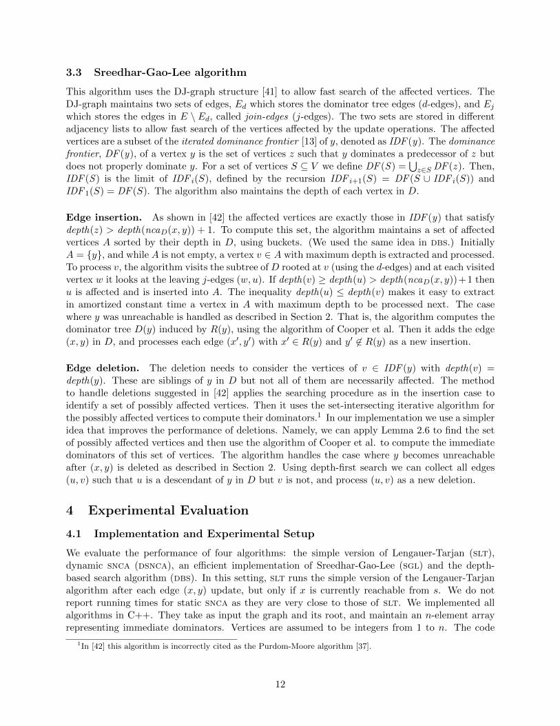
Edge deletion. The deletion needs to consider the vertices of v ∈ IDF (y) with depth(v) =depth(y). These are siblings of y in D but not all of them are necessarily affected. The methodto handle deletions suggested in [42] applies the searching procedure as in the insertion case toidentify a set of possibly affected vertices. Then it uses the set-intersecting iterative algorithm forthe possibly affected vertices to compute their dominators.1 In our implementation we use a simpleridea that improves the performance of deletions. Namely, we can apply Lemma 2.6 to find the setof possibly affected vertices and then use the algorithm of Cooper et al. to compute the immediatedominators of this set of vertices. The algorithm handles the case where y becomes unreachableafter (x, y) is deleted as described in Section 2. Using depth-first search we can collect all edges(u, v) such that u is a descendant of y in D but v is not, and process (u, v) as a new deletion.

4 Experimental Evaluation

4.1 Implementation and Experimental Setup

We evaluate the performance of four algorithms: the simple version of Lengauer-Tarjan (slt),dynamic snca (dsnca), an efficient implementation of Sreedhar-Gao-Lee (sgl) and the depth-based search algorithm (dbs). In this setting, slt runs the simple version of the Lengauer-Tarjanalgorithm after each edge (x, y) update, but only if x is currently reachable from s. We do notreport running times for static snca as they are very close to those of slt. We implemented allalgorithms in C++. They take as input the graph and its root, and maintain an n-element arrayrepresenting immediate dominators. Vertices are assumed to be integers from 1 to n. The code

1In [42] this algorithm is incorrectly cited as the Purdom-Moore algorithm [37].

12

was compiled using g++ v. 3.4.4 with full optimization (flag -O4). All tests were conducted onan Intel Core i7-920 at 2.67GHz with 8MB cache, running Windows Vista Business Edition. Wereport CPU times measured with the getrusage function. Running times include allocation anddeallocation of arrays and linked lists, as required by each algorithm, but do not include readingthe graph from an input file. Our source code is available upon request.

4.2 Instances and Evaluation

Our test set consists of a sample of graphs used in [26], graphs taken from the Stanford LargeNetwork Dataset Collection [43], and road networks [14]. We report running times for a repre-sentative subset of the above test set, which consist of the following: the control-flow graph uloopfrom the SPEC 2000 suite created by the IMPACT compiler, the foodweb baydry, the VLSI circuits38584 from the ISCAS’89 suite, the peer-to-peer network p2p-Gnutella25, and the road networkrome99. We constructed a sequence of update operations for each graph by simulating the updateoperations as follows. Let m be the total number of edges in the graph. We define parametersi and d which correspond, respectively, to the fraction of edges to be inserted and deleted. Thismeans that mi = i ∗m edges are inserted and md = d ∗m edges are deleted, and the flow graphinitially has m′ = m − mi edges. The algorithms build (in static mode) the dominator tree forthe first m′ edges in the original graph file and then they run in dynamic mode. For i = d = 0,sgl reduces to the iterative algorithm of Cooper et al. [11], whilst dsnca and dbs reduce to snca.The remaining edges are inserted during the updates. The type of each update operation is chosenuniformly at random, so that there are mi insertions interspersed with md deletions. During thissimulation that produces the dynamic graph instance we keep track of the edges currently presentin the graph. If the next operation is a deletion then the edge to be deleted is chosen uniformly atrandom from the edges in the current graph.

4.3 Evaluation

The experimental results for various combinations of i and d are shown in Table 1. The reportedrunning times for a given combination of i and d is the average of the total running time takento process ten update sequences obtained from different seed initializations of the srand function.With the exception of baydry with i = 50, d = 0, in all instances dsnca and dbs are the fastest.In most cases, dsnca is by a factor of more than 2 faster than slt. sgl and dbs are much moreefficient when there are only insertions (d = 0), but their performance deteriorates when there aredeletions (d > 0). For the d > 0 cases, dbs and dsnca have similar performance for most instances,which is due to employing the deletion test of Lemma 3.1. On the other hand, sgl can be evenworse than slt when d > 0. For all graphs except baydry (which is extremely sparse) we observe adecrease in the running times for the i = 50, d = 50 case. In this case, many edge updates occurin unreachable parts of the graph. (This effect is more evident in the i = 100, d = 100 case, so wedid not include it in Table 1.) Overall, dbs achieves the best performance. dsnca is a good choicewhen there are deletions and is a lot easier to implement.

13

graph instance insertions deletions slt dsnca sgl dbsi d

uloop 10 0 315 0 0.036 0.012 0.008 0.006n = 580 0 10 0 315 0.039 0.012 0.059 0.012m = 3157 10 10 315 315 0.065 0.017 0.049 0.014

50 0 1578 0 0.129 0.024 0.013 0.0120 50 0 1578 0.105 0.024 0.121 0.023

50 50 1578 1578 0.067 0.015 0.041 0.033100 0 3157 0 0.178 0.033 0.023 0.019

0 100 0 3157 0.120 0.026 0.136 0.050

baydry 10 0 198 0 0.010 0.002 0.004 0.003n = 1789 0 10 0 198 0.014 0.003 0.195 0.004m = 1987 10 10 198 198 0.020 0.003 0.012 0.005

50 0 993 0 0.034 0.009 0.007 0.0080 50 0 993 0.051 0.007 0.078 0.012

50 50 993 993 0.056 0.006 0.033 0.020100 0 1987 0 0.048 0.004 0.013 0.015

0 100 0 1987 0.064 0.010 0.095 0.022

rome99 10 0 887 0 0.261 0.106 0.027 0.017n = 3353 0 10 0 887 0.581 0.252 1.861 0.291m = 8870 10 10 887 887 0.437 0.206 0.863 0.166

50 0 4435 0 0.272 0.106 0.049 0.0310 50 0 4435 1.564 0.711 4.827 0.713

50 50 4435 4435 0.052 0.016 0.074 0.065100 0 8870 0 0.288 0.103 0.068 0.056

0 100 0 8870 1.274 0.613 4.050 0.639

s38584 10 0 3449 0 6.856 2.772 0.114 0.096n = 20719 0 10 0 3449 7.541 4.416 15.363 4.803m = 34498 10 10 3449 3449 6.287 3.586 5.131 2.585

50 0 17249 0 9.667 3.950 0.228 0.1500 50 0 17249 10.223 5.671 17.543 5.835

50 50 17249 17249 0.315 0.107 0.342 0.291100 0 34498 0 10.477 4.212 0.301 0.285

0 100 0 34498 10.931 6.056 18.987 6.016

p2p-Gnutella25 10 0 5470 0 38.031 9.295 0.167 0.123n = 22687 0 10 0 5470 38.617 13.878 38.788 16.364m = 54705 10 10 5470 5470 72.029 21.787 37.396 14.767

50 0 27352 0 129.668 37.206 0.415 0.2560 50 0 27352 133.484 49.730 131.715 51.764

50 50 27352 27352 60.776 27.996 28.478 19.448100 0 54705 0 136.229 39.955 0.724 0.468

0 100 0 54705 128.738 54.405 139.449 44.064

Table 1: Average running times in seconds for 10 seeds. The best result in each row is bold.

14

References

[1] F. E. Allen and J. Cocke. Graph theoretic constructs for program control flow analysis.Technical Report IBM RC 3923, IBM T.J. Watson Research, 1972.

[2] S. Allesina and A. Bodini. Who dominates whom in the ecosystem? Energy flow bottlenecksand cascading extinctions. Journal of Theoretical Biology, 230(3):351–358, 2004.

[3] S. Alstrup, D. Harel, P. W. Lauridsen, and M. Thorup. Dominators in linear time. SIAMJournal on Computing, 28(6):2117–32, 1999.

[4] S. Alstrup and P. W. Lauridsen. A simple dynamic algorithm for maintaining a dominatortree. Technical Report 96-3, Department of Computer Science, University of Copenhagen,1996.

[5] M. E. Amyeen, W. K. Fuchs, I. Pomeranz, and V. Boppana. Fault equivalence identificationusing redundancy information and static and dynamic extraction. In Proceedings of the 19thIEEE VLSI Test Symposium, March 2001.

[6] S. Baswana, K. Choudhary, and L. Roditty. Fault tolerant reachability for directed graphs.In Yoram Moses, editor, Distributed Computing, volume 9363 of Lecture Notes in ComputerScience, pages 528–543. Springer Berlin Heidelberg, 2015.

[7] A. L. Buchsbaum, L. Georgiadis, H. Kaplan, A. Rogers, R. E. Tarjan, and J. R. Westbrook.Linear-time algorithms for dominators and other path-evaluation problems. SIAM Journal onComputing, 38(4):1533–1573, 2008.

[8] A. L. Buchsbaum, H. Kaplan, A. Rogers, and J. R. Westbrook. A new, simpler linear-timedominators algorithm. ACM Trans. on Programming Languages and Systems, 20(6):1265–96,1998. Corrigendum appeared in 27(3):383-7, 2005.

[9] M. D. Carroll and B. G. Ryder. Incremental data flow analysis via dominator and attributeupdate. In Proc. 15th ACM POPL, pages 274–284, 1988.

[10] S. Cicerone, D. Frigioni, U. Nanni, and F. Pugliese. A uniform approach to semi-dynamicproblems on digraphs. Theor. Comput. Sci., 203:69–90, August 1998.

[11] K. D. Cooper, T. J. Harvey, and K. Kennedy. A simple, fast dominance algorithm. SoftwarePractice & Experience, 4:110, 2001.

[12] R. Cytron, J. Ferrante, B. K. Rosen, M. N. Wegman, and F. K. Zadeck. Efficiently comput-ing static single assignment form and the control dependence graph. ACM Transactions onProgramming Languages and Systems, 13(4):451–490, 1991.

[13] R. Cytron, J. Ferrante, B. K. Rosen, M. N. Wegman, and F. K. Zadeck. Efficiently computingstatic single assignment form and the control dependence graph. ACM Trans. Program. Lang.Syst., 13:451–490, 1991.

[14] C. Demetrescu, A. Goldberg, and D. Johnson. 9th DIMACS Implementation Challenge -Shortest Paths, 2006.

[15] D. Firmani, L. Georgiadis, G. F. Italiano, L. Laura, and F. Santaroni. Strong articulationpoints and strong bridges in large scale graphs. Algorithmica, 74(3):1123–1147, 2016.

15

[16] W. Fraczak, L. Georgiadis, A. Miller, and R. E. Tarjan. Finding dominators via disjoint setunion. Journal of Discrete Algorithms, 23:2–20, 2013.

[17] H. N. Gabow. A poset approach to dominator computation. Unpublished manuscript, 2013.

[18] L. Georgiadis. Testing 2-vertex connectivity and computing pairs of vertex-disjoint s-t pathsin digraphs. In Proc. 37th Int’l. Coll. on Automata, Languages, and Programming, pages738–749, 2010.

[19] L. Georgiadis. Approximating the smallest 2-vertex connected spanning subgraph of a directedgraph. In Proc. 19th ESA, pages 13–24, 2011.

[20] L. Georgiadis, G. F. Italiano, L. Laura, and N. Parotsidis. 2-edge connectivity in directedgraphs. In Proc. 26th ACM-SIAM Symp. on Discrete Algorithms, pages 1988–2005, 2015.

[21] L. Georgiadis, G. F. Italiano, L. Laura, and N. Parotsidis. 2-vertex connectivity in directedgraphs. In Proc. 42nd Int’l. Coll. on Automata, Languages, and Programming, pages 605–616,2015.

[22] L. Georgiadis, L. Laura, N. Parotsidis, and R. E. Tarjan. Dominator certification and inde-pendent spanning trees: An experimental study. In Proc. 12th Int’l. Symp. on ExperimentalAlgorithms, pages 284–295, 2013.

[23] L. Georgiadis, L. Laura, N. Parotsidis, and R. E. Tarjan. Loop nesting forests, dominators,and applications. In Proc. 13th Int’l. Symp. on Experimental Algorithms, pages 174–186, 2014.

[24] L. Georgiadis and R. E. Tarjan. Finding dominators revisited. In Proc. 15th ACM-SIAMSymp. on Discrete Algorithms, pages 862–871, 2004.

[25] L. Georgiadis and R. E. Tarjan. Dominator tree certification and divergent spanning trees.ACM Transactions on Algorithms, 12(1):11:1–11:42, November 2015.

[26] L. Georgiadis, R. E. Tarjan, and R. F. Werneck. Finding dominators in practice. Journal ofGraph Algorithms and Applications (JGAA), 10(1):69–94, 2006.

[27] M. Gomez-Rodriguez and B. Scholkopf. Influence maximization in continuous time diffusionnetworks. In 29th International Conference on Machine Learning (ICML), 2012.

[28] M. S. Hecht and J. D. Ullman. Characterizations of reducible flow graphs. Journal of theACM, 21(3):367–375, 1974.

[29] M. Henzinger, S. Krinninger, and V. Loitzenbauer. Finding 2-edge and 2-vertex stronglyconnected components in quadratic time. In Proc. 42nd Int’l. Coll. on Automata, Languages,and Programming, pages 713–724, 2015.

[30] G. F. Italiano, L. Laura, and F. Santaroni. Finding strong bridges and strong articulationpoints in linear time. Theoretical Computer Science, 447(0):74–84, 2012.

[31] R. Jaberi. Computing the 2-blocks of directed graphs. RAIRO-Theor. Inf. Appl., 49(2):93–119,2015.

[32] R. Jaberi. On computing the 2-vertex-connected components of directed graphs. DiscreteApplied Mathematics, 204:164 – 172, 2016.

16

[33] T. Lengauer and R. E. Tarjan. A fast algorithm for finding dominators in a flowgraph. ACMTrans. on Programming Languages and Systems, 1(1):121–41, 1979.

[34] W. Di Luigi, L. Georgiadis, G. F. Italiano, L. Laura, and N. Parotsidis. 2-connectivity in di-rected graphs: An experimental study. In Proc. 17th SIAM Meeting on Algorithm Engineeringand Experimentation, pages 173–187, 2015.

[35] E. K. Maxwell, G. Back, and N. Ramakrishnan. Diagnosing memory leaks using graph miningon heap dumps. In Proc. 16th ACM SIGKDD Int. Conf. on Knowledge Discovery and DataMining, KDD ’10, pages 115–124, 2010.

[36] K. Patakakis, L. Georgiadis, and V. A. Tatsis. Dynamic dominators in practice. In Proc. 16thPanhellenic Conference on Informatics, pages 100–104, 2011.

[37] P. W. Purdom, Jr. and E. F. Moore. Algorithm 430: Immediate predominators in a directedgraph. Communications of the ACM, 15(8):777–778, 1972.

[38] L. Quesada, P. Van Roy, Y. Deville, and R. Collet. Using dominators for solving constrainedpath problems. In Proc. 8th International Conference on Practical Aspects of DeclarativeLanguages, volume 3819 of Lecture Notes in Computer Science, pages 73–87. Springer, 2006.

[39] G. Ramalingam and T. Reps. An incremental algorithm for maintaining the dominator treeof a reducible flowgraph. In Proc. 21st ACM POPL, pages 287–296, 1994.

[40] V. C. Sreedhar. Efficient program analysis using DJ graphs. PhD thesis, School of ComputerScience, McGill University, September 1995.

[41] V. C. Sreedhar and G. R. Gao. Computing phi-nodes in linear time using DJ graphs. J. Prog.Lang., 3(4):191–213, 1995.

[42] V. C. Sreedhar, G. R. Gao, and Y. Lee. Incremental computation of dominator trees. ACMTrans. Program. Lang. Syst., 19:239–252, 1997.

[43] Stanford network analysis platform (SNAP). http://snap.stanford.edu/.

[44] R. E. Tarjan. Finding dominators in directed graphs. SIAM Journal on Computing, 3(1):62–89,1974.

[45] R. E. Tarjan. Testing flow graph reducibility. J. Comput. Syst. Sci., 9(3):355–365, 1974.

[46] R. E. Tarjan. Efficiency of a good but not linear set union algorithm. Journal of the ACM,22(2):215–225, 1975.

17