AN EXPERIMENTAL INVESTIGATION OF AN ELECTRICAL … · AN EXPERIMENTAL INVESTIGATION OF AN...
136
Department of Mechanical and Aerospace Engineering AN EXPERIMENTAL INVESTIGATION OF AN ELECTRICAL STORAGE HEATER IN THE CONTEXT OF STORAGE TECHNOLOGIES Author: Ignacio Becerril Romero Supervisor: Dr Paul Strachan A thesis submitted in partial fulfilment for the requirement of the degree Master of Science Sustainable Engineering: Renewable Energy Systems and the Environment 2013
Transcript of AN EXPERIMENTAL INVESTIGATION OF AN ELECTRICAL … · AN EXPERIMENTAL INVESTIGATION OF AN...

Department of Mechanical and Aerospace Engineering
AN EXPERIMENTAL INVESTIGATION OF AN
ELECTRICAL STORAGE HEATER IN THE
CONTEXT OF STORAGE TECHNOLOGIES
Author: Ignacio Becerril Romero
Supervisor: Dr Paul Strachan
A thesis submitted in partial fulfilment for the requirement of the degree
Master of Science
Sustainable Engineering: Renewable Energy Systems and the Environment
2013

Copyright Declaration
This thesis is the result of the author’s original research. It has been composed by the
author and has not been previously submitted for examination which has led to the
award of a degree.
The copyright of this thesis belongs to the author under the terms of the United
Kingdom Copyright Acts as qualified by University of Strathclyde Regulation 3.50.
Due acknowledgement must always be made of the use of any material contained in,
or derived from, this thesis.
Signed: Ignacio Becerril Romero Date: 22nd
September 2013

i
Abstract
This project is divided in two different parts: an investigation of energy storage and an
experimental analysis of a storage heater.
The “20 20 20” targets dictate that the share of renewables in EU’s energy
consumption has to be increased to a 20% by the year 2020 (European Commission,
2012). More flexibility needs to be added to the grid in order to integrate the
increasing amount of variable generation. Energy storage is especially well suited to
respond to this challenge (Teller et al., 2013). However, the role that storage is to play
in the future grid needs to be evaluated meticulously. A detailed investigation of the
services that storage can provide to the grid and of the main storage technologies is
carried out in this thesis. The analysis shows that storage is a very valuable element of
the energy grid since it can provide numerous services at the same time. It plays a
fundamental role within the integration of renewables and is particularly useful
combined with wind power to avoid curtailment and minimum generation constrains.
In addition, it is realised that only a combination of different storage technologies can
deliver all the services that energy storage will need to provide in the future.
State-of-the-art storage heaters can provide demand side management (DSM) services
in small isolated grids with significant wind generation. The charging periods of the
heater can be scheduled by the utility provider based on wind output and demand
forecasts. At the same time, storage heaters can also provide frequency response.
However, they present some features that may affect their performance. No relevant
publications were found about the topic, so an experimental analysis of the
thermophysical properties of the storage medium and of the temperature distribution
inside the core of the heater is performed. The first shows that the specific heat and
conductivity of the storage material are higher than expected with values of CP = 1.58
J/g·K and k = 4.3 W/m·K. It is concluded that the storage material presents good
qualities for heat storage. On the other hand, the temperature distribution is shown to
be very inhomogeneous during a standard charging cycle. Nevertheless, the method
used overestimates the average temperature of the core of the heater by a 50%
showing that a 3D approach is necessary to study absolute temperatures. Likewise, the
data obtained are insufficient to study the performance of the heater as DSM and, due
to the lack of time and equipment, this is left as future work. cxcxcxcxcxcxcxcxcxcxc

ii
Acknowledgements
I would like to express my gratitude to the following:
My supervisor, Dr Paul Strachan, for his kind support, encouragement and guidance
over the course of the project.
My ‘second supervisor’, Katalin Svehla, for her kindness, support, guidance, and for all
the effort she put into having a new insulation panel delivered.
Chris Cameron, for securing the heater to the wall, cutting samples from the bricks and,
in general, for his help and approachability.
Fiona Sillars, for performing the analysis of the samples and giving me valuable
information about the results and the experimental procedure.
Jim Doherty, for his continuous good mood and his efficient work ordering and
supplying everything I needed throughout the project.
A very special thanks goes to John Redgate for his priceless help. The technical part of this
project would have been impossible without him. He has fixed the heater every time
anything failed (something that, unfortunately, has happened too often in this project),
made lots of thermocouples and installed new controls in the heater in addition to ‘a long
etcetera’; and he has always done it with a smile in his face.
I would also like to thank:
My parents, José Luis and Elda, for supporting me in everything I do and giving me the
opportunity to study this MSc.
My grandmothers, Aurora and Ángeles, for their unconditional love; and, although they
are not here anymore, I also want to thank my grandfathers, Pepe y Pascual, for all the
love they gave me and all the things I learnt from them.
The rest of my family and my friends in Spain. I could not have got so far without them.
My friends in Glasgow for making this year a wonderful experience.
My dear friend Preet, for sharing so many late nights with me at the Livingstone Tower
and for his help and support in the last days of this project.
And, finally, my girlfriend, Anita, for her love and for dealing with my stress and bad
mood during this stressful project and for trying to help and support me always in every
way she can.
iii
Contents
1. Introduction ............................................................................................................... 1
2. Energy Storage .......................................................................................................... 4
2.1 Applications of Energy Storage within the Energy Grid ................................... 4
2.1.1 Introduction ................................................................................................ 4
2.1.2 Electric Supply Applications ...................................................................... 5
2.1.3 Ancillary Services Applications/Frequency Response Services ................ 5
2.1.4 Grid System Applications ........................................................................... 9
2.1.5 End User Applications .............................................................................. 11
2.1.6 Renewables Integration Applications ....................................................... 13
2.2 Storage and Wind Power ................................................................................. 17
2.2.1 Introduction .............................................................................................. 17
2.2.2 Wind uncertainty ...................................................................................... 18
2.2.3 Minimum generation constrains ............................................................... 19
2.3 Location of storage .......................................................................................... 20
2.3.1 Separated generation and storage ............................................................. 21
2.3.2 Co-location of generation and storage ...................................................... 22
2.3.3 Bottom line ............................................................................................... 23
2.4 Energy Storage Technologies .......................................................................... 24
2.4.1 Introduction .............................................................................................. 24
2.4.2 Mechanical energy storage ....................................................................... 24
2.4.3 Chemical energy storage .......................................................................... 31
2.4.4 Electrochemical energy storage - Batteries and supercapacitors.............. 33
2.5 Conclusions ...................................................................................................... 39
2.6 Thermal Energy Storage (TES) ....................................................................... 41
2.6.1 Introduction .............................................................................................. 41
iv
2.6.2 Sensible heat ............................................................................................. 42
2.6.3 Latent heat ................................................................................................ 44
2.6.4 Thermo-chemical storage ......................................................................... 47
2.6.5 Applications .............................................................................................. 48
2.6.6 Conclusions .............................................................................................. 49
2.7 Summary .......................................................................................................... 52
3. Storage Heaters ....................................................................................................... 54
3.1 Storage heater basics ........................................................................................ 54
3.1.1 Introduction .............................................................................................. 54
3.1.2 Structure, types and operation of storage heaters ..................................... 56
3.2 Storage heaters as demand side management (DSM) ...................................... 60
3.2.1 Demand side management ........................................................................ 60
3.2.2 Dynamic storage heaters capabilities for DSM ........................................ 64
4. Experimental Analysis of a Storage Heater ............................................................ 67
4.1 The SM heater .................................................................................................. 67
4.2 Thermal properties of the storage medium ...................................................... 69
4.2.1 Experimental set-up .................................................................................. 70
4.2.2 Results ...................................................................................................... 73
4.2.3 Discussion and conclusions ...................................................................... 78
4.3 Temperature distribution .................................................................................. 79
4.3.1 Experimental set-up .................................................................................. 80
4.3.2 Experiments and results ............................................................................ 81
4.3.3 Storage capacity ...................................................................................... 104
4.3.4 Outer surface temperature ...................................................................... 108
4.4 Discussion ...................................................................................................... 109
4.4.1 Remark about the validity of the experimental results ........................... 109
4.4.2 SM heater as a ‘night storage heater’ ..................................................... 109

v
4.4.3 SM heater as demand side management ................................................. 113
4.4.4 Energy stored and heat losses ................................................................. 115
4.5 Conclusions and further work ........................................................................ 117
4.5.1 Temperature distribution ........................................................................ 117
4.5.2 Energy stored and heat losses ................................................................. 119
4.5.3 Summary ................................................................................................. 119
5. REFERENCES ...................................................................................................... 121
vi
List of figures
Figure 1 - Matching supply and demand. Load following. .............................................. 6
Figure 2- Area regulation ................................................................................................. 7
Figure 3- Reactance .......................................................................................................... 9
Figure 4- Diurnal variability of solar radiation. ............................................................. 14
Figure 5 - Renewable energy firming ............................................................................. 16
Figure 6- Power scheduled and wind prediction ............................................................ 19
Figure 7 – Separated generation and storage. ................................................................. 22
Figure 8 – Co-location of generation and storage. ......................................................... 23
Figure 9 - Storage technologies ...................................................................................... 24
Figure 10- Typical operation of a CAES plant. .............................................................. 25
Figure 11 - Flywheel structure. ...................................................................................... 27
Figure 12 - Typical PHS plant ........................................................................................ 30
Figure 13 - Chemical storage cycles............................................................................... 32
Figure 14 – Chemical storage efficiency ........................................................................ 32
Figure 15 - Basic cell battery structure ........................................................................... 33
Figure 16 – Redox Flow battery. .................................................................................... 37
Figure 17 - Applications of electrochemical storage. ..................................................... 38
Figure 18 - Heat storage methods and media. ................................................................ 42
Figure 19 - Structure of a static storage heater ............................................................... 57
Figure 20 - Structure of a dynamic storage heater.......................................................... 58
Figure 21 - Static vs dynamic storage heater .................................................................. 59
Figure 22 - Main objectives of DSM .............................................................................. 61
Figure 23 - Storage heater as DSM. Charging scheduling ............................................. 65
Figure 24- SM heater structure and main elements ........................................................ 68
Figure 25 - Volumetric heat capacity of different materials .......................................... 69
Figure 26 - Temperature increase in the rear face of a sample in LFA .......................... 71
Figure 27 - LFA 427 structure ........................................................................................ 72
Figure 28 - Specific heat of synthetic magnetite ............................................................ 76
Figure 29 - Thermal conductivity of MgO ..................................................................... 78
Figure 30 – Transversal location of TCs ........................................................................ 81
Figure 31 - Initial test. TC distribution ........................................................................... 81
Figure 32 – Second test. Experiment 1. TC distribution. ............................................... 85
vii
Figure 33 - Second test. Experiment 2. TC distribution. ................................................ 86
Figure 34 – Finals tests. New approach for the estimation of the temperature of the
bricks .............................................................................................................................. 90
Figure 35 – Final tests. TC distribution .......................................................................... 92
Figure 36 - 3D effect experiment. TC location ............................................................ 107
List of graphs
Graph 1 - Density of magnetite used in the SM heater .................................................. 73
Graph 2 – Storage medium. Thermal diffusivity ............................................................ 74
Graph 3 – Storage medium. Specific heat ...................................................................... 75
Graph 4 – Storage medium. Thermal conductivity ........................................................ 77
Graph 5 – Initial test. TC temperature distribution. ....................................................... 83
Graph 6 - Second test. Reference TCs comparison in experiments 1 and 2................... 86
Graph 7 - Second test. TC temperatures in experiments 1 (left) and 2 (right) ............... 87
Graph 8 - Second test. Brick temperature distribution ................................................... 88
Graph 9 – Final tests. Comparison between second test approach and the new one using
the results from the second test ...................................................................................... 91
Graph 10 - Side thermocouples ...................................................................................... 93
Graph 11 – TC comparison between different rows....................................................... 94
Graph 12 - Temperature evolution of every brick within the core of the SM heater ..... 95
Graph 13 – Minimum, maximum and average core temperature ................................. 102
Graph 14 - Measurement of the dispersion of temperatures inside the core. Descriptive
statistics ........................................................................................................................ 103
Graph 15 - 3D effect experiment. Top of brick 19 ....................................................... 107
Graph 16 - Outer surface temperature .......................................................................... 108
Graph 17 - Average temperature change rate ............................................................... 112

viii
List of tables
Table 1 - Heat capacities of common TES media at 20°C ............................................. 44
Table 2 - PCM and sensible heat media properties ........................................................ 46
Table 3- TES systems comparison ................................................................................. 50
Table 4 - Energy storage technologies comparison ........................................................ 53
Table 5 - SM heater technical data ................................................................................. 67
Table 6 - Power, resistance, voltage and intensity of the SM heater ............................ 104
Table 7 - Parameters of linear variation of CP .............................................................. 105
Table 8 - Estimation of the stored energy using average temperatures ........................ 106
List of equations
Equation 1 - Thermal diffusivity .................................................................................... 70
Equation 2 - LFA thermal diffusivity ............................................................................. 71
Equation 3 - Cp estimation by comparison with standard reference sample.................. 71
Equation 4 - Mean value of CP from Graph 3. ............................................................... 76
Equation 5 - Total power input to the SM heater ......................................................... 105
Equation 6 - Estimation of the energy stored in a brick ............................................... 105
Equation 7 - Linear variation of CP (T) ....................................................................... 105
Equation 8 - Resolution of an integration step ............................................................ 105
1
1. Introduction In December 2008, the European Parliament and the European Council agreed upon the
so called Climate and Energy Package, more commonly known as the 20 20 20 targets.
These are a set of binding legislation which aims to ensure the European Union meets
its ambitious climate and energy targets for 2020 (European Commission, 2012). The
three key objectives of this legislation are, namely:
A reduction in greenhouse gas emissions of at least 20% below 1990 levels
An increase of the share of renewable energy to 20% in the overall energy
consumption
An improvement of the overall EU’s energy efficiency of a 20%
The second bullet point of the previous list implies that the energy network will have to
cope with high amounts of unpredictable and variable renewable generation. The
current energy grid only possesses a limited degree of flexibility provided, mainly, by
conventional rapid cycling gas turbines or hydro power plants (Denholm, 2012).
Increasing the share of RES in the generation mix will inevitably require a higher
flexibility to avoid situations in which, from time to time, generation largely exceeds
demand or vice versa, and the problems this can pose to transmission and distribution
networks.
Energy storage is especially well suited to respond to this challenge and ensure a
continued security of energy supply at any time by storing energy in times of excess
supply and releasing power when there is not enough generation.
However, in order to understand the role that storage will play in the future energy grid
and, especially, within the integration of renewable energy, it is first necessary to
investigate and understand the following topics:
1. What are the services that energy storage currently provides to the grid
2. What are the potential services that storage could further provide
3. How these services are currently carried out without energy storage
4. What are the present and future technologies that can provide these services

2
It is difficult to find an exhaustive analysis where all these elements are reviewed and
gathered together although it is fundamental to understand the potential of energy
storage. Thus, this situation has motivated the first part of this thesis in which a deep
investigation of all the subjects listed above is presented.
Demand side management (DSM) is another effective way of providing flexibility to
the grid but its large-scale implementation is very complex (Strbac, 2008). In contrast,
isolated communities with small self-managed energy grids (like islands) and abundant
wind resources offer a great potential for DSM.
These communities are often not connected to the gas grid. Thus, electric heating
commonly represents a high percentage of the total energy consumption. Storage
heaters are the preferred choice for electric heating due to their reduced running costs
when combined with off-peak tariffs. Moreover, state-of-the-art models feature
automated charging controls that can be remotely programmed by the utility provider.
This allows their use as DSM.
In already mentioned small isolated communities with significant amounts of wind
generation, two main types of DSM services are identified for ‘smart’ storage heaters:
Charging scheduling - utility providers can use wind output and demand
forecasts to schedule optimum charging times in the heater.
Frequency response - by monitoring the frequency of the grid, heaters can
automatically detect imbalances and modify their energy consumption.
However, storage heaters also present a number of issues that can affect their
performance as DSM:
Core temperature distribution – ceramic bricks used in storage heaters as storage
medium exhibit low thermal conductivities that can lead to very uneven
temperature distributions in the core of the heater.
Standing losses – storage heaters exhibit unwanted heat losses that reduce their
efficiency.
Human factors – a wrong programming of the heater can result in significant
amounts of wasted energy.
A ‘smart’ storage heater was experimentally analysed in the second part of this thesis.

3
The thermophysical properties of the storage medium determine the behaviour of the
storage heater to a large extent. However, there is a lack of relevant publications about
this topic. This motivated the first part of the experimental analysis in which the main
thermal properties of the storage material are analysed in detail.
Likewise, the same situation occurs with the temperature distribution inside the core of
the heater. The second part of the experimental analysis, thus, investigates the
temperature distribution and studies how it can affect the overall performance of the
heater. In addition, it is used to assess its storage capacity and standing losses.

4
2. Energy Storage
2.1 Applications of Energy Storage within the
Energy Grid
2.1.1 Introduction
Energy storage plays a very important role in the current grid providing services such as
operating reserves, energy arbitrage and frequency control just to mention a few.
The main historical reason for research on and application of energy storage was the
need of matching demand and supply. Energy could be stored during off-peak periods
from base-load plants (large coal and nuclear plants, mainly) and be released during
peak periods to meet demand. Pumped hydro storage (PHS) plants were developed for
this purpose and, actually, they are still the dominant energy storage technology today.
According to Strbac et al. (2012), PHS currently provides the 99% of the global energy
storage capacity.
In the 1970s, there was a strong interest in energy storage due to dramatic increase in
the price of oil entailed by the oil crisis. Many of the current PHS plants were built
during that period since they were a cheaper way to meet peak demand than fossil-fuel
based peaking plants (Denholm et al., 2010). Likewise, many other storage
technologies were also researched and developed like flywheels, several types of
batteries, capacitors or electromagnetic superconducting storage (DOE, 1977).
However, the drop in the price of natural gas set and end to this situation and global
interest shifted from energy storage technologies to flexible generation gas turbines,
both open and combined cycle, which became the cheapest peaking technology
(Denholm et al., 2010).
Nevertheless, energy storage has remained as a key element of the energy grid thanks to
the numerous services it can provide. These can be classified into five different classes
(Eyer and Corey, 2010): electric supply, ancillary services, grid system, end user and
renewable integration applications. In this section, the services most widely discussed in
the literature are listed and briefly explained in order to investigate the importance of
energy storage in the current and future energy grid.

5
2.1.2 Electric Supply Applications
Electric energy time-shift/Energy arbitrage
Off-peak low-cost energy is stored during low demand periods (especially at night) and
released to meet peak demand. The energy stored comes mainly from base-load plants
that are desirable to be operated continuously at maximum capacity since they achieve
their highest efficiency and lowest running-costs when working in this regime.
Energy arbitrage favours the use of efficient and expensive base-load plants instead of
inefficient peaking plants. Thus, fuel consumption, emissions and overall running costs
are reduced. The capital cost of the global system may be also reduced because of the
fewer peaking plants required to meet the peak demand. (Walawalkar et al., 2004)
Electric supply capacity
Strongly related to the previous one, stored energy is used to ensure a reliable
generation capacity to meet the demand during peak periods. Energy storage could be
used to defer and/or to reduce the need to buy new generation capacity and/or to ‘rent’
generation capacity in the wholesale electricity marketplace (Eyer and Corey, 2010).
2.1.3 Ancillary Services Applications/Frequency Response
Services
Any imbalance between electric power generation and consumption results in a
frequency change within the entire network of the synchronous area. Stored energy can
be used to maintain the frequency of the grid constant (i.e. match supply and demand) in
case of predicted or unpredicted events. The energy stored is usually referred to as
operating reserves (Denholm et al., 2010). Unlike the applications just mentioned
above, the response time of the operating reserves has to be low. Due to the long time
required to put a generator online and the fuel expenses associated to it, the usual
solution to deal with these issues is the use of partially loaded generators synchronised
with the grid that can detect and correct variations in the frequency of the grid (sensitive
mode); and, also, by load reductions from some industrial customers (Strbac et al.,
2012). There are three basic frequency response services: load following, area

6
regulation and reserve capacity. Voltage control and black-start are also two services
highly related to frequency and, thus, they are also included in this section.
Load Following
In order to operate the energy grid, supply must be able to match demand at every time.
Since demand varies throughout the day, a variable output supply is necessary as well.
The figure below depicts how demand is met by different types of generation and the
role that load-following generation plays within the total generation mix.
Figure 1 - Matching supply and demand. Load following. Ref: Eyer and Corey (2010)
The traditional solution to provide load-following services is to use of partially loaded
generators synchronised with the frequency of the grid that can increase (follow-up) or
decrease (follow-down) their output rapidly. However, partially loaded generators are
less fuel efficient and have higher emissions than generators operating at their rated
output. Maintenance costs associated to modulated generators are also higher than those
of constant output generators. (Callaway and Hiskens, 2011)
Storage may be an attractive alternative to most generation-based load following for at
least three reasons (Eyer and Corey, 2010):
Storage has superior part-load efficiency
Efficient storage can use twice its rated capacity (i.e. it can stop discharging and
start charging at the same time) providing an efficient service both for follow-up

7
(energy is discharged from storage) and follow-down (energy is charged)
operations.
Storage output can be varied very rapidly (e.g., output can change from 0 to
100% or from 100 to 0% within seconds)
Area regulation
Regulation is the response to momentary and unpredicted variations in the energy
demand (Denholm et al., 2010). The difference with load following lies on its
momentary and unpredictable nature as well as on its smaller amplitude (see Figure 2).
However, area regulation is usually addressed by the use of partially loaded thermal
generators just like load following (Eyer and Corey, 2010). It has been already
remarked that the efficiency of partially loaded generators is quite low and implies high
fuel consumption and air emission rates.
Energy storage is particularly useful for area regulation for the three reasons mentioned
above. The fast response and the capability of providing twice its rated capacity (charge
plus discharge) are vital for area regulation due to the rapid and random nature of the
frequency variations (see figure below).
Figure 2- Area regulation. Ref. Denholm et al., (2010)

8
Electric supply reserves capacity
Every electric power system needs to have some reserve generation to back-up
unexpected losses of power, e.g. a generator failure. These reserves are known as
contingency reserves (Denholm et al., 2010). There are three types of contingency
reserves (Eyer and Corey, 2010):
Spinning reserves - they are the first type of reserves used when a shortfall
occurs. They are comprised by generators that are online (synchronised) but
unloaded so they can increase their output very rapidly.
Supplemental reserves - they are used after all spinning reserves are online and
can be available within 10 minutes. Supplemental reserves are not synchronized
with the grid.
Back-up Supply - It can pick up load within one hour. Its role is, essentially, a
backup for spinning and supplemental reserves.
Again, its rapid response and firm supply makes storage an ideal option for contingency
reserves. Furthermore, spinning reserves need to be online even when they are not
needed while storage technologies do not start discharging until the fault is detected.
Black-start capability
National Grid (n.d.) defines a black start as “the procedure to recover from a total or
partial shutdown of the transmission system which has caused an extensive loss of
supplies. This entails isolated power stations being started individually and gradually
being reconnected to each other in order to form an interconnected system again.”
Only power plants with no or very low start-up energy needs have the ability to black-
start (Zach et al., 2012). PHS plants and diesel engines are commonly used as black
start units. However, other bulk energy storage technologies could also be used for this
type of service.
Voltage support
Inductors and capacitors in AC systems produce a phenomenon called reactance.
Energy is stored and released in the form of magnetic (inductors) and electric
(capacitors) fields which, in turn, generate opposing electromotive forces. As a result,

9
current stops being in phase with voltage and, thus, the effective voltage and power
delivered by the grid is reduced (see figure below).
Time Mag
nit
ud
e
Current
Voltage
Power delivered
Maximum power
deliverable (if in phase)
Figure 3- Reactance
Voltage must be maintained within an acceptable range for both customer and grid
equipment to function properly. This can be controlled by generating or absorbing
reactive power to compensate the effect of reactance. Both generation and transmission
equipment can be used for this purpose. However, when generators are required to
supply excessive amounts of reactive power, their real-power production must be
curtailed. (Kirby and Hirst, 1997)
According to Eyer and Corey (2010), many major power outages are attributable to
problems transmitting reactive power to load centres. Using distributed storage near
load to create reactive power can be a particularly good alternative since this type of
power cannot be transmitted efficaciously over long distances (Kirby and Hirst, 1997).
2.1.4 Grid System Applications
Transmission support
The electricity transmitted through transmission and distribution (T&D) networks is not
a perfect sine wave. It can present several anomalies like voltage dips, unstable voltage
or sub-synchronous resonances that can compromise the performance of transmission.

10
The rapid response of storage technologies is well-suited for this purpose. Energy
storage can be used to improve the performance of T&D systems by correcting the
disturbances and anomalies in the transmitted electricity (Eyer and Corey, 2010).
Transmission congestion relief
Transmission congestion decreases the system efficiency and increases electricity prices
through congestion charges or locational marginal pricing. It occurs when peak load is
higher than the transmission system’s maximum capacity. Furthermore, congestion
increases the need of enlarging transmission lines and has an elevated cost associated.
(Samant, 2011)
Energy storage systems can be deployed downstream from the congestion point. They
would be charged during low demand periods and discharge during peak demand to
alleviate congestion and, thus, mitigate upwards pressure on electric prices and defer
and/or eliminate the need for further transmission expansion. (Eyer and Corey, 2010;
Samant, 2011)
Transmission and distribution upgrade deferral
T&D systems are designed for maximum peak demand. However, this high demand
typically occurs only during a few hours a year (Denholm et al., 2010). The upgrading
of T&D systems to accommodate the increasing peak demand can be delayed or even
avoided if energy storage is placed near load (downstream from the T&D overloaded
node) to be used during peak times (Nourai, 2007). It can report great savings since the
elevated capital cost of building new substations, transformers, lines, etc. would be
avoided. At the same time, energy storage near load can also reduce the large line-losses
that take place during high peak demands (Nourai et al., 2008; Denholm and Sioshansi,
2009).
It is important to note that a small amount of storage can provide enough incremental
capacity to defer the need for a large investment in T&D equipment (Eyer and Corey,
2010). This can be observed in the following example provided by EPRI-DOE (2003,
p.53):
Assuming a load increase of 2.5% per year, the upgrade of a 9 MWac system (in
California) to 12 MWac could be deferred for one year by building a storage plant of

11
just 225 kW. This would result in 150000$ benefit. If the cost of storage is equal or less
to this quantity, the repayment period of the storage plant would be equal or lower than
one year.
In addition, not only T&D upgrading is deferred but also the lifetime of the T&D
equipment can be substantially improved by reducing maximum load or load swings.
(EPRI-DOE, 2003)
Substation on-site power
Energy storage provides power at electric utility substations for switching components
as well as for substation communications and control equipment when the grid is not
energized. (Sandia Corporation, 2012)
The vast majority of these systems use lead-acid batteries, mostly vented valve-
regulated, with 5% of systems being powered by NiCd batteries. Lead-acid batteries are
a low-cost and extremely entrenched in the market technology and users are satisfied
with their lifetime and operational performances. Therefore, advances in energy storage
technologies are not likely to make an important change in this service. (Eckroad et al.,
2004)
2.1.5 End User Applications
It should be noted that the storage systems described in this section need to use time-
varying prices and/or be very site-specific in order to be economically feasible for end
users (Denholm et al., 2010). TOU and demand charge management will be further
discussed when talking about demand side management in section 3.2.1.
Time-of-use (TOU) energy cost management
TOU energy cost management is the equivalent to energy arbitrage but at a customer
level. Costumers use and/or store energy during off-peak periods, when the price of
electricity is low, in order to get an economic benefit. Obviously, this requires that the
electricity provider offers a time-variable tariff like UK’s “Economy 7 tariff” which
charges electricity cheaper overnight (for seven hours) than during the day.

12
Two technologies widely used for this purpose are storage heaters and hot water
cylinders. Electricity is stored in the form of thermal energy during night and released
during the day to provide space heating and hot water respectively.
Demand charge management
Similarly to the previous service, utility users can use storage to avoid the use of
electricity during peak hours that may be penalised with “demand charges”. This
usually affects only to large electricity consumers (more than 2 MWh/month). These
costumers are forced to have installed a demand meter that takes readings every 15
minutes. Accordingly, their electricity tariff varies every 15 minutes too. (National Grid,
2005).
Energy can be stored throughout the day and be used to reduce the overall demand
during peak periods. Therefore, storage can make a significant difference in the energy
bill for large customers by avoiding expensive demand charges at peak hours.
Electric service reliability
Energy storage can be used as on-site back-up supply in the event of a power outage. It
should provide enough energy to ride through outages of extended duration; to complete
an orderly shutdown of processes; or to transfer to on-site generation resources (Eyer
and Corey, 2010). All these options lead to a highly reliable electric service and can be
of particular interest for costumers like hospitals or other facilities where energy supply
is critical for their operation. Energy storage can complement (or even substitute)
traditional back-up generators (usually diesel generators) providing, in addition, a very
rapid response.
UPS (uninterruptible power supply) units used to protect computers, data centres or
telecommunication equipment are a good example of this service. They are an extended
technology and can provide power almost instantaneously.
Electric service power quality
Voltage spikes, dips or harmonics are common issues in the electricity supply and they
are said to worsen the power quality. They can produce malfunction in electrical devices
and can even cause severe damage in sensitive equipment. Storage is commonly used

13
by the customer at load site to buffer and protect sensitive equipment (Denholm et al.,
2010).
2.1.6 Renewables Integration Applications
Most of renewable energy generation is highly unpredictable and the variability of its
energy output poses control, response and other energy management challenges to the
utility operators. Energy storage has the capability of firming and backing up the
variable and intermittent nature of renewables by smothering its supply profile and
extending its useful generation time (Denholm et al., 2010). That way, storage could
also help to stabilise the price of renewable energy avoiding its curtailment when its
price is too low (Denholm and Sioshansi, 2009).
Storage appears, thus, to be the ideal solution to accommodate variable generation.
However, the role that it will play in the future grid is not so clear. The viability of
storage will depend on many factors like the penetration and type of renewable
generation or the cost of deployment of storage versus other technologies. There are
other ways of integrating variable generation within the grid like flexible generation,
interconnection and demand side management (Strbac et al., 2012). Either way, surely
energy storage is very beneficial when combined with renewables.
Renewables energy time-shift
One of the main issues of renewable generation is that it is usually not produced when it
is needed. As an example, wind generation usually blows most intensely at night and
early morning (Bentek Energy, 2010). Energy generated during off-peak periods has a
very low price in the energy market. Storage could be used to store this low-price
energy and sell (release) it during on-peak times when it is more valuable (Eyer and
Corey, 2010).
The characteristics of time-shifting vary from technology to technology. Wind, solar
and base-load renewables are briefly explained to illustrate these differences
Wind
As stated above, wind usually has a large output overnight. In addition to its low value,
excessive wind generation during off-peak periods can also cause minimum load
14
constrains which are a serious operational challenge (this will be explained in section
2.2.3). Energy could be stored overnight and be released during peak demand so it is
more valuable and minimum load constrains are avoided.
For the case of wind generation, the required discharge duration ranges from two and
one-half hours to as much as four hours, depending on the amount of energy from wind
generation that occurs during on-peak times. (Eyer and Corey, 2010)
Solar
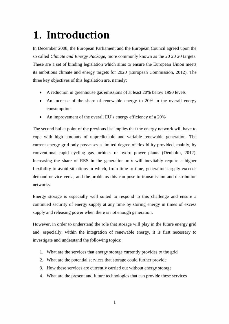
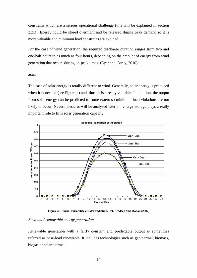
The case of solar energy is totally different to wind. Generally, solar energy is produced
when it is needed (see Figure 4) and, thus, it is already valuable. In addition, the output
from solar energy can be predicted to some extent so minimum load violations are not
likely to occur. Nevertheless, as will be analysed later on, energy storage plays a really
important role to firm solar generation capacity.
Figure 4- Diurnal variability of solar radiation. Ref. Pradeep and Mohan (2007)
Base-load renewable energy generation
Renewable generation with a fairly constant and predictable output is sometimes
referred as base-load renewable. It includes technologies such as geothermal, biomass,
biogas or solar thermal.

15
Time-shift in this case works very similar to wind power. Energy is stored during off-
peak periods (usually at night) and used at peak times when it is more valuable.
Renewables capacity firming
As it has been stated many times before, one of the major concerns of renewable
generation is its unpredictable intermittency. It has been already explained how these
output variations imply the use of rapid-response dispatchable generators as back-up
supply such as open cycle gas turbines.
The combination of variable generation and storage can provide a constant output from
intermittent sources of energy. This is known as capacity firming. Wind and solar
energy are the most extended technologies and, thus, for which storage offers a higher
potential.
Solar PV
PV generation suffers from two equally important types of intermittency: short-duration
and diurnal (Eyer and Corey, 2010).
Short-duration intermittency accounts for temporary shading of the PV panels due to
objects or, more importantly, clouds (Sayeef et al., 2012). When shading occurs, the
output from the solar panels decreases substantially. Storage can be used to “fill” these
momentary generation gaps so the overall output remains constant (Eyer and Corey,
2010).
On the other hand, diurnal intermittency of solar generation is basically due to the
variable amount of radiation that PV panels receive during the day as the sun moves in
the sky. A typical profile of this variability can be found in Figure 4. It can be observed
that the bulk of solar generation occurs during on-peak times. It is especially during on-
peak periods when it is important for the grid operators to count with constant energy
outputs. Storage can be used to provide this service by discharging during on-peak
times when the power output is lower than the rated power of the plant.
Energy storage plays, thus, a fundamental role to make PV generation reliable and
useful.

16
Wind
Wind power also presents short-duration and diurnal intermittency although less
markedly than in the case of solar. Short-duration intermittency is due to rapid
variations in the wind speed and diurnal intermittency comes from the tendency of wind
to blow stronger during some parts of the day (or night) (Bentek Energy, 2010).
Storage could be used, as in the case of solar, when the output of the power plant falls
below its rated power during on-peak periods to provide a constant and reliable output.
Capacity of storage needed for firming of renewables
The capacity of the storage system needed for firming of renewables depends on the
maximum power drop-off (Eyer and Corey, 2010). The next figure illustrates the
meaning of drop-off.
Figure 5 - Renewable energy firming. Ref: Eyer and Corey, 2010
In the case of the figure above, a storage power of 0.34 kW would be necessary to
provide enough firming since it is the maximum difference between rated power of the
plant and the real power output.
Eyer and Corey (2010) indicate that the duration of the discharge should be from one
and a half to two hours for solar and from three to four hours for wind.

17
Bottom line
Energy time-shifting and capacity firming are the only two applications of storage that
can be considered specific to renewable generation. However, every service listed
before is totally connected with and useful for the integration of renewable energy. E.g.
variable generation poses load-following and area regulation challenges, needs
contingency reserves, can worsen power quality, produce congestion in T&D systems,
etc. Therefore, storage and renewable generation are very interrelated and will be even
more with the growth of variable generation.
2.2 Storage and Wind Power
2.2.1 Introduction
Wind energy is growing very fast. According to Carrington (2013) it grew a 20%
globally in 2012. Thus, it is the renewable technology which is starting to pose the
biggest integration challenges.
According to Denholm et al. (2010) the integration costs of wind power arise mainly
from:
Area regulation - the increased costs that result from providing short-term
ramping resulting from wind deployment.
Load-following - the increased costs that result from providing the hourly
ramping requirements resulting from wind deployment.
Wind uncertainty - the increased costs that result from having a suboptimal mix
of units online because of errors in the wind forecast.
However, different studies (Denholm et al., 2010) show that area regulation and load-
following do not have a significant impact in the overall integration costs. This is due to
the current capacity of the grid to supply variable output in order to match demand.
Thus, wind uncertainty is the main cause for wind integration costs.
18
2.2.2 Wind uncertainty
Supply needs to be planned in advance according to the forecasted demand. Only the
precise number of generators required to meet demand are scheduled so that they are
online at the right time. This is known as unit commitment. Large base-load generators
need a particularly good planning due to the long time and high fuel requirements
necessary to bring them online. The combination of base-load, load-following and
peaking generators that provides the right supply with the highest efficiency is usually
referred to as the optimal generation mix.
Because of the unpredictable nature of wind, wind power is often regarded as an
unexpected reduction in the demand profile more than like part of the supply scheme
(Denholm et al., 2010). Therefore, wind power with relatively high degree of
penetration becomes a very important part of the planning for unit commitment (see
Figure 6 left). If there is a large difference between real wind output and the prediction,
the following scenarios can occur[1]
:
If the wind output is lower than predicted (Figure 6 centre), there is not enough
scheduled supply to meet demand. Back-up generation (e.g. contingency reserves) need
to be brought online and/or some large costumers be asked to reduce their load. This
scenario represents elevated costs that could have been avoided by scheduling cheaper
base-load generation.
On the other hand, if the wind out is higher than predicted (Figure 6 right), there is an
excess of supply. Customers will be encouraged to use electricity by very low, zero, or
even negative prices and/or wind production will need to be curtailed. Again, the costs
associated to this situation are high. The expenses of scheduling too much large base-
load generation are high and, at the same time, fuel-free wind power is being wasted.
Storage could significantly reduce the costs associated to prediction inaccuracy by
providing additional supply in the case of an underestimation (Figure 6 right) or by
absorbing the excess of generation in the case of an overestimation (Figure 6 centre)
avoiding supply shortages and undesirable wind power curtailment respectively.
1 A similar analysis can be found in Denholm et al., (2010)

19
Nevertheless, storage is expensive and its implementation should be economically
evaluated. As an example, many renewable integration studies (Denholm et al., 2010)
show that with a wind generation up to a 30% of the total there is no need for additional
storage.
Figure 6- Power scheduled and wind prediction
2.2.3 Minimum generation constrains
It is often assumed that renewable generation only displaces load-following generation
(see Figure 1). This is true only for low penetration levels. Load-following generators
are designed to modulate their output so renewable energy does not pose a significant
integration problem. It can be accommodated easily by just varying the output of load-
following generators properly.
Nevertheless, in some countries wind power starts to represent a high percentage of the
total generation. Just to mention a couple of examples, wind power accounted for 18.1%
of the total generation during 2012 in Spain (Red Eléctrica de España, 2012) and
30.08% in Denmark (Energinet, 2013). For elevated amounts of wind generation, it is
possible that not only load-following but also base-load generation needs to reduce its
output in order to accommodate wind. However, it is not an easy task and an
unsuccessful base-load modulation can lead to wind power curtailment. A study by
20
Ackermann et al. (2009) shows that wind curtailment is a common issue in the Danish
energy power system during periods of high wind output.
This is usually referred to in the literature as minimum generation constrains. Its origin
lies in the fact that base-load generators are not designed to be modulated and,
furthermore, they have a minimum output they need to provide to operate safely. As an
example, large coal-fired power plants are often restricted to operating in the range of
50-100% of full capability, although the lack of experience cycling these plants makes
that limit very uncertain (Denholm et al., 2010).
Logically, renewable energy curtailment due to minimum generation constrains will
occur more frequently with higher penetrations of wind power. This can put a limit to
the growth of renewable energy. The only way of avoiding this situation is to add
flexibility to the grid. Conventional rapid-response generators, interconnection, demand
side management and storage are the most common solutions proposed to do this
(Lannoye, 2012).
Energy storage can be a key element in avoiding curtailment and reducing (or even
eliminating) minimum generation constrains. Storage technologies can absorb excess
generation, that would be wasted (curtailed) otherwise, and shift it to times of high
demand. Furthermore, Denholm et al., (2010) suggest that storage could effectively
replace base-load generation as it provides firm capacity. This would eliminate
minimum loading limitations totally.
Minimum generation constrains are very site-specific Thus, the cost of storage
technology versus other options will define its ultimate role in the future grid in every
specific case.
2.3 Location of storage
It has been shown in previous sections that energy storage is likely to be a key element
of the future grid because of all the useful services it can provide as well as its capacity
to accommodate large amounts of variable generation. However, it has not been
discussed so far a crucial aspect of storage: its optimum location.

21
It is quite common to think of storage units coupled directly to renewable generators.
Energy could be stored in times of excess generation and released when necessary for
every individual renewable energy plant. This would result in lots of renewable and
dispatchable generators, what seems a desirable situation. Surprisingly, if that was case,
the overall efficiency of the global energy power system would be compromised.
However, there are some situations in which it is beneficial to tie generation and storage
together.
Micro-grids and highly distributed storage are not considered in this discussion.
However, they can provide very useful services and add flexibility to the grid. The role
that storage heaters can play as demand side management distributed storage will be
analysed later on.
2.3.1 Separated generation and storage
It is easy to see that the way storage operates when coupled to a single generator is
totally analogous to energy arbitrage (see section 2.1.2) but in an individual basis.
Nevertheless, energy arbitrage is more efficient when the energy operator can choose
what type of generation to store based on cost and efficiency (Denholm et al., 2010). If
arbitrage is restricted to only one energy source, the optimal generation mix (the one
that ensures maximum generation efficiency) is lost and the flexibility of the overall
system decreases.
The concept behind storage location is resource aggregation. This concept is quite easy
to understand when talking about energy demand. The demand of a single customer can
vary very abruptly and is highly unpredictable. Using a power plant to supply electricity
to a single customer would be, thus, quite absurd and inefficient. There would be many
times of excess and lack of power supply while, at the same time, other customers
would be in the opposite situation. Hence, if many different loads are aggregated, the
combined demand profile is much smoother and easy to match.
The same situation is applicable to storage. Let’s use the case of wind power. The
output of a single plant is highly variable. If a storage facility is tied to a single plant it
will be discharging when there is not enough wind and charging when there is an
excess. However, other plants can be in the opposite situation at the same time. Thus, it
would be very likely that energy was being stored at some facilities and discharged at
22
others simultaneously. This is a total waste of the capabilities of storage resources and,
in addition, the losses associated with the storage process make the operation highly
inefficient.
Likewise, the supply profile for an aggregation of wind power plants located at different
places tends to be smoother since the wind has different blowing patterns at different
locations.
For those reasons, an aggregation of both loads and variable generation sources would
lead to an optimum use of storage resources reducing, consequently, both capital and
running costs.
Besides energy arbitrage, it is of extreme importance to note that a storage plant not tied
to a variable generation plant can also provide many other high-value grid services as it
was explained in the previous section (see section 2.1). Therefore, co-locating
generation and storage is also a waste of the potential of storage technologies.
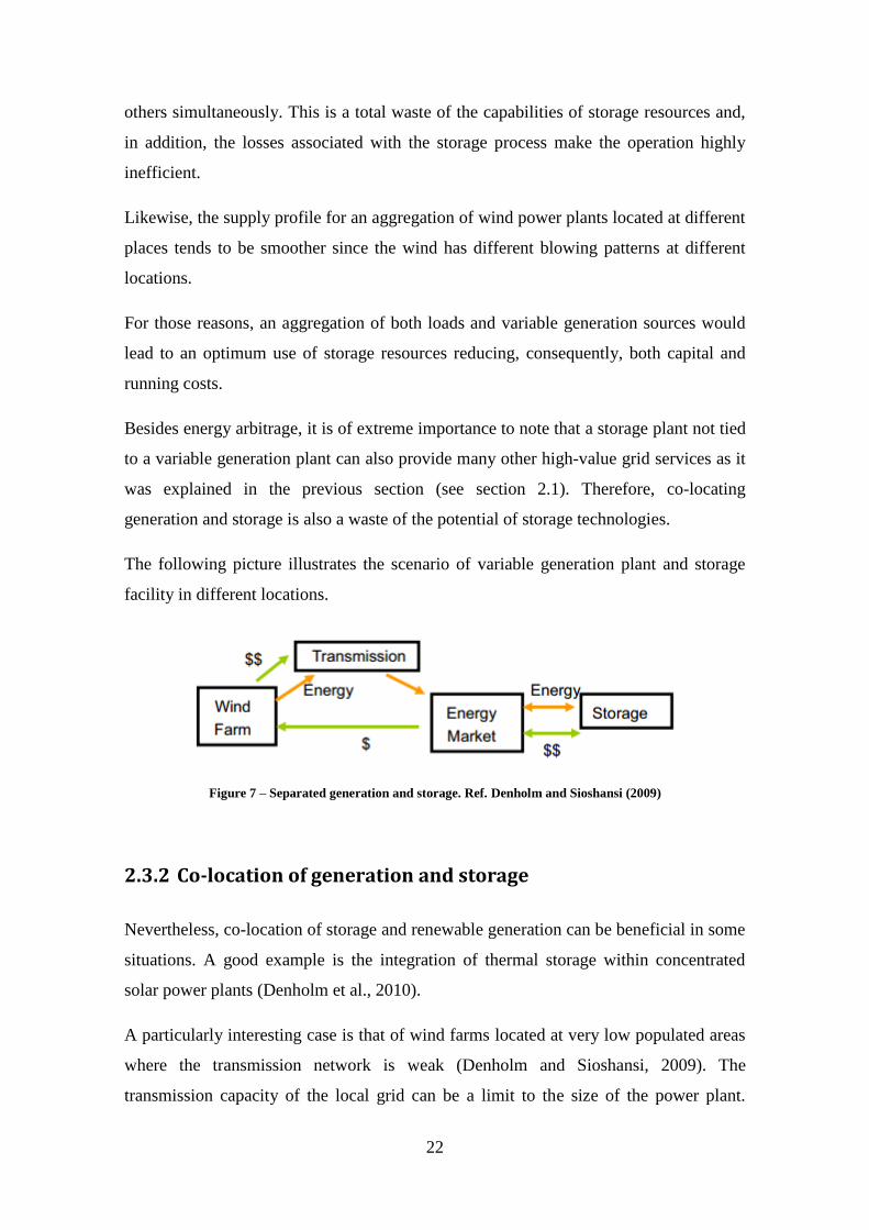
The following picture illustrates the scenario of variable generation plant and storage
facility in different locations.
Figure 7 – Separated generation and storage. Ref. Denholm and Sioshansi (2009)
2.3.2 Co-location of generation and storage
Nevertheless, co-location of storage and renewable generation can be beneficial in some
situations. A good example is the integration of thermal storage within concentrated
solar power plants (Denholm et al., 2010).
A particularly interesting case is that of wind farms located at very low populated areas
where the transmission network is weak (Denholm and Sioshansi, 2009). The
transmission capacity of the local grid can be a limit to the size of the power plant.

23
However, it has been already mentioned (see section 2.1.4) that upgrading T&D lines
has an elevated capital cost.
Integration of storage within the wind farm (i.e. upstream the transmission line) can
downsize the maximum power supplied by the plant and, consequently, it can avoid the
upgrading of the transmission line. The question here is whether the reduced
transmission costs exceed the penalties associated with a suboptimal use of the energy
storage plant (Denholm and Sioshansi, 2009).
The following picture illustrates the scenario of generation and storage co-location
Figure 8 – Co-location of generation and storage. Ref. Denholm and Sioshansi (2009)
2.3.3 Bottom line
A good bottom line to this discussion can be found at Denholm et al. (2010): “Just as
loads are balanced in aggregate, the net load in the future grid – after all variable
generation sources are included – will be balanced by a mix of conventional generation,
plus flexibility options that include energy storage”.

24
2.4 Energy Storage Technologies
2.4.1 Introduction
So far, only the services that storage can provide to the grid have been analysed.
However, it is equally important to examine the different storage technologies used for
those services, their performance and potential.
The figure below gives an idea of the wide range of technologies available for energy
storage. This section investigates the most common ones found in the literature focusing
mainly on how they work, their positive and negative characteristics, their limitations
and the services they can provide to the operation of grid.
Figure 9 - Storage technologies. Ref. IEC (2011)
2.4.2 Mechanical energy storage
Compressed air energy storage (CAES)
CAES plants store energy in the form of air elastic potential energy (compressed air).
Electricity is taken from the grid to drive a compressor. Compressed air is then stored in
tanks above the ground or in underground geologic formations (caves, mines…). To
convert the stored energy back into electricity, the compressed air is heated and
expanded through a gas turbine attached to a generator. The diagram below illustrates a
typical operation CAES plant.

25
Figure 10- Typical operation of a CAES plant. Source: http://www.ridgeenergystorage.com/
Heat is released as result of the compression process. Nevertheless, the air must be
preheated before expansion in order to avoid ice formation in the turbine (due to the
Joule-Thomson effect). Natural gas or other fuels are used for this purpose. If the heat
arising from the compression is released to the atmosphere, the storage process is called
diabatic CAES and has a 40-50% efficiency (Teller et al., 2013). On the other hand, that
heat could be stored and used to preheat the air before its expansion. This concept is
called adiabatic CAES and should result in round-trip efficiencies of up to 65% (EPRI-
DOE, 2003).
The main features of CAES systems are: an efficient partial load operation, the ability to
start up without an external power input, reaching of full power within minutes and
quick transition from generation to compression mode. (Chen et al., 2013)
Applications
The main advantage of CAES is its large capacity when using underground storage.
This large scale potential makes CAES a very suitable technology for future energy
arbitrage like PHS. However, CAES is not only suitable for large but also for small
scale storage applications. For example, decentralised CAES technology could be
deployed at difficult accessible places with considerable share of fluctuating renewable
electricity generation. (Teller et al., 2013)

26
It can be particularly useful in combination with wind power. Markets are expected in
northern Europe close to off-shore wind farms (Teller et al., 2013). CAES can be
applied within wind farms to balance generation and demand and can be used to reduce
the size (and capital cost) of transmission lines. Some authors, like Denholm and
Sioshansi (2009), have already explored the potential of co-location of wind power and
CAES with positive results.
Regarding standard grid services, EPRI-DOE (2003) lists the following services
currently provided by the only CAES facility in the U.S.: load management, ramping,
peak generation, synchronous condenser duty and spinning reserve duty. In addition
CAES can be applied to provide secondary and tertiary balancing power as well as
black start capability (Teller et al., 2013).
Limitations
Similarly to PHS, the major barrier for CAES is the need of favourable geographic
formations for its deployment. (Chen et al., 2013)
Another limitation when compared to PHS or other storage technologies is that CAES
requires a gas combustion turbine to operate. This leads to emissions that make CAES
less environmentally friendly. (Chen et al., 2013)
In addition, the low efficiency of diabatic CAES is also a limitation for investment in
this technology. Nevertheless, the new CAES schemes proposed, like adiabatic CAES,
are likely to improve the efficiency of CAES to levels comparable to those of PHS and
reduce emissions. (Chen et al., 2013; Teller et al., 2013)
Finally, CAES is today not economically viable when only single applications are used
to generate revenues. This means that CAES will probably have to act on different
markets simultaneously in order to justify the necessary investments, limiting its
potential (Teller et al., 2013).
Flywheels
Flywheels store energy in the form of kinetic energy of a spinning mass, called a rotor.
The amount of energy stored in a spinning body depends only on its rotational speed

27
and on its mass. Motor-generators are used to convert electricity into kinetic energy and
vice versa.
Figure 11 - Flywheel structure. Ref. Hadjipaschalis (2009)
The following features make flywheels an attractive storage technology:
They can act as high-power devices, which absorb and release energy at a high
rate. Most power flywheel products can provide from 100 to 2000 kWac for a
period of time ranging between 5 and 50 seconds (EPRI-DOE, 2003).
They have a long life, which is unaffected either by the frequency of cycling or
by overcharging or deep discharges. Most developers estimate cycle life in
excess of 100,000 full charge-discharge cycles (EPRI-DOE, 2003).
Energy and power density in flywheels are almost independent variables, as
opposed to other systems like batteries. They have thus flexibility in design and
unit size (Dell and Rand, 2001).
They have high round-trip efficiencies: 80-85% (Teller et al., 2013)
They work very well as power devices and are well suited for applications which
involve the frequent charge and discharge of modest quantities of energy at
high-power ratings. (Dell and Rand, 2001)
They require very little maintenance.
They are constructed from readily available materials.
They have no environmental impact in use or in recycling.
28
Conversely, flywheel systems have high self-discharge ratings, must be housed in
robust containment for safety reasons and require high engineering precision
components which currently results in a relatively high cost (Strbac et al., 2012)
Applications
Flywheels are mainly used nowadays for power quality applications, mainly for short-
term bridging through power disturbances or from one power source to an alternate
source. (EPRI-DOE, 2003)
Other applications include frequency and voltage support, renewables firming and
stabilization, transport applications for light rail and large road vehicles and as UPSs for
industrial uses. (Denholm et al., 2010; Teller et al., 2013; EPRI-DOE, 2003; Strbac et
al., 2012)
For the latter application, flywheels are usually sold as a clean, reliable and long cycle
life alternative to batteries. However, some studies show the potential of combining
flywheels and batteries to improve the reliability as well as the overall efficiency and
lifetime of power conditioning systems (Richey, 2004).
For renewable integration applications, flywheels are of particular interest for localized
storage of electricity generated by wind turbines and photovoltaic arrays. A flywheel-
based buffer storage could remove the need for downstream power electronics to track
the fluctuations in power output improving the overall efficiency of the system.
Rechargeable batteries would seem to be a more appropriate storage medium and, in
fact, these are widely used today. However, a battery–flywheel combination (as just
stated above) is worthy of consideration for this application. (Dell and Rand, 2001)
Limitations
The most significant limitation of flywheels lies in their relatively modest capability for
energy storage although they work very well for high power applications. An increase
of power and energy density is required in order to reduce the high investment costs and
make them competitive against other technologies (Liu and Jiang, 2007)
Technical restrictions arise mainly from bearings and friction that limit the potential of
flywheels. The bearings, which support the flywheel rotor, are a significant source of

29
friction, the most life-limiting part and if they fail there can be serious incidents. Some
developers have introduced magnetic bearings to improve all those issues.
Finally, another limitation comes from the heat generated by the friction between the
rotor and the medium it which it is enclosed. Besides leading to energy losses, it can
increase the temperature of some parts of the flywheel system reducing the safety and
reliability of the system. Many different cooling systems have been proposed to address
this problem, like hydrogen cooling similar to the one use in large generators (EPRI-
DOE, 2003).
Pumped hydro storage (PHS)
PHS is the most established storage technology. It represents around 99% of the global
grid scale energy storage capacity. It is also the storage technology with highest storage
capacities. It can be sized up to several GW and its efficiency is usually around 70-85%
although it depends on the operation and characteristics of the plant. (Strbac et al.,
2012)
The basic elements of a PHS plant include the turbine-pump equipment attached to a
motor-generator, a waterway, an upper reservoir and a lower reservoir (see Figure 12).
Pure PHS plants only shift the water between reservoirs. Though, there also exist
combined plants that can generate their own electricity like conventional hydroelectric
plants through natural steam-flow besides pumping storage (Hadjipaschalis et al., 2009).
The main advantages of PHS are its very long lifetime and practically unlimited cycle
stability of the installation. It also has a high flexibility and can ramp up to full
production capacity within minutes. The typical discharge times range from several
hours to a few days. However, it has a relatively low energy density and requires either
a very large body of water or a large variation in height and its capital cost is very high.
(IEC, 2011; Teller et al., 2013; Hadjipaschalis et al., 2009)

30
Figure 12 - Typical PHS plant. Source:
http://www.bbc.co.uk/bitesize/standard/physics/energy_matters/generation_of_electricity/revision/3/
Applications
The main application of PHS is energy arbitrage. By storing energy in times of low
demand, it enables fossil-fired and renewable energy plants to be operated at their most
efficient levels more often. Apart from the economic benefit arbitrage reports, it also
helps to reduce emissions and fuel consumption. (Teller et al., 2013)
Furthermore, its flexibility in power and short response time make PHS a useful tool to
balance the grid during unplanned outages of other power plants acting as non-spinning
reserves. Thus, PHS plants are already being currently used for both primary and
secondary regulation in the European electricity grid. (Teller et al., 2013; IEC, 2011)
Limitations
The main weakness that limits the future potential of PHS is the inherent dependence on
very specific topographical conditions for its deployment. It also has a large
environmental impact since it requires an extensive use of land (IEC, 2011).
In addition, the future potential of PHS will be also determined by the capacity of this
technology to improve its flexibility to accommodate the increasing amount of variable

31
generation and even to help with the ultra-fast regulation that will be needed with the
introduction of large HVDC electric highways. (Teller et al., 2013)
2.4.3 Chemical energy storage
Chemical energy storage comprises, mainly, the use of excess electricity generation to
produce hydrogen via water electrolysis. The hydrogen produced from this process can
be used directly or be further transformed into synthetic natural gas (SNG) by reacting it
with CO2.
Hydrogen
A chemical storage system based on hydrogen consists of an electrolyser to produce
hydrogen from pure water electrolysis, a storage tank to store the hydrogen produced
and a fuel cell to combine the hydrogen with air (oxygen) to obtain electricity again.
In addition to fuel cells, gas motors, gas turbines and combined cycles of gas and steam
turbines are in discussion for power generation. (IEC, 2011)
SNG
In this case, after the electrolysis there is a process called methanation in which
hydrogen is reacted with CO2 to obtain methane. This methane can then be stored or
released into the gas grid.
The most common source of CO2 considered for methanation are fossil-fuelled power
plants, some large industries and biogas plants. In order to minimize losses, it is
recommended the co-location of the electrolyser, the CO2 source and the storage tanks
(or pipelines).

32
Figure 13 - Chemical storage cycles. Ref. Teller et al. (2013)
Efficiency
The efficiency of the complete cycle can be as high as 40%, similar to coal fired steam
power plants (Teller et al., 2013). The most significant losses take place during
electrolysis, methanation and re-electrification (see figure below).
Figure 14 – Chemical storage efficiency. Ref. Teller et al. (2013)
The overall efficiency is lower than other bulk energy storage technologies such as
CAES, PHS or Li-ion batteries. However, chemical energy storage is the only concept
that allows storage of large amounts of energy, up to the TWh range, and for greater
periods of time – even as seasonal storage (IEC, 2011).

33
Applications
The high energy density and the potential large scale of storage facilities make chemical
storage suitable for energy arbitrage and seasonal storage. Moreover, electrolysers have
the ability to react within a second or lower upon changes in electricity supply/demand,
both up and down (Teller et al., 2013). They are therefore well suited for provision of
ancillary services for the future electrical grid with high penetration of variable
generation.
In addition, hydrogen and SNG can be used directly as fuels for transport and industrial
applications as well as for synthesising several chemical compounds (Teller et al., 2013)
or could be used on gas and steam turbines in peaking power plants (IEC, 2011).
Limitations
The limitations for this technology arise from its elevated cost and as well as the
inexistent infrastructure although there are many technological and efficiency aspects
that need to be overcome too.
2.4.4 Electrochemical energy storage - Secondary batteries and
supercapacitors
Electrochemical batteries use reversible redox reactions to store energy. They consist of
different cells that contain two electrodes and an electrolyte material (see figure below).
Figure 15 - Basic cell battery structure. Source:
http://www.spring8.or.jp/en/news_publications/research_highlights/no_49/
When a battery discharges, negative ions in the electrolyte near one of the anodes
supply electrons (oxidation) while positive ions near the cathode accept electrons
34
(reduction). The process is reversed to charge the battery, i.e. ions are created in the
electrolyte.
Lead-acid
They are the world’s most widely used battery type and have been commercially
deployed since about 1890 (IEC, 2011).
They are low-cost, easy to recharge, easy to recycle and they have a huge availability.
However, they have many short-comes like low specific energy and power, short cycle
life, high maintenance requirements and environmental hazards associated with lead and
sulphuric acid. Some of these disadvantages have been overcome by improvements in
chemistry and design. (EPRI-DOE, 2003)
Their most commons applications are as starter batteries in vehicles, storage for stand-
alone PV houses and they can be even found in wind farms to smoother output
fluctuations. (IEC, 2011)
Nickel based batteries (NiFe, NiCd, NiMH)
Nickel based batteries were invented around 1900 and are therefore almost as old as
lead–acid. These alkaline batteries have not been as successful as the later because of
their higher cost. (Dell and Rand, 2001)
Nickel-iron batteries suffer from numerous defects and thus have never been very
popular However their high extreme durability and relative tolerance of nearly any kind
of abuse, physical or operational, have made the suitable for several applications like
mining or railroad signalling. (EPRI-DOE, 2003; Battery University, 2013)
By contrast, nickel–cadmium have an overall better performance than lead–acid and
other beneficial features like flat discharge voltage, long life, overcharge capability, low
water maintenance and high reliability (Dell and Rand, 2001). However, they have a
high cost and, because of the toxicity of cadmium, these batteries are presently used
only for stationary applications in Europe and they have been prohibited for consumer
use since 2006 (IEC, 2011).
NiMH batteries have all the positive properties of NiCd and much higher energy
densities but their maximal nominal capacity is ten times less when compared to NiCd

35
and lead acid. They have been extensively replaced by lithium ion batteries although
hybrid vehicles operate almost exclusively with NiMH batteries as these are far safer
than lithium ion batteries. NiMH batteries currently cost about the same as lithium ion.
(IEC, 2011)
Lithium-ion batteries
Lithium-ion batteries are currently the most important storage technology in mobile
applications. They have a high efficiency (95 % - 98 %) and energy density, a cell
voltage three times higher than Ni-based batteries and can achieve nearly any discharge
time which makes them a very flexible and universal storage technology (IEC, 2011). In
addition, they are low maintenance batteries and have little self-discharge (Battery
University, 2013)
However, they are fragile, have aging problems and require built-in voltage and charge
level control protection circuits to maintain a safe operation. As a consequence of this,
Li-ion batteries have a high cost and are challenging for large-scale applications.
However, the costs are likely to drop with mass production. Likewise, safety, storage
capacity and performance are likely to improve in the near future as an intense research
is being carried out on this technology in the present time. (IEC, 2011; Battery
University, 2013)
Since lithium-ion batteries are currently still expensive, they can only compete with lead
acid batteries in those applications which require short discharge times (e.g. as primary
control backup). (IEC, 2011)
Sodium-based batteries (NaS, ZEBRA) batteries
NaS is a high-temperature battery that uses molten sulphur and sodium as electrodes
and solid beta alumina ceramic as electrolyte. The operational temperature usually
ranges from just below 300°C to near 400°C so the electrodes remain molten (Dell and
Rand, 2001). They have a long lifetime and discharge times, an efficiency around 75%
and fast response. Thus, they can be used and have been already applied (mainly in
Japan) in power quality, grid stabilisation and time-shifting applications (IEC, 2011).
One of the drawbacks of the battery is the need of a heat source and a good insulation in
order to maintain its operational temperature. This is usually made by using battery’s

36
own energy, decreasing its overall efficiency (IEC, 2011). However, the major concerns
are related to safety. If there was a fracture and sodium and sulphur mixed, there would
and exothermal reaction with a potential fire hazard that would damage the whole
battery, not just the faulty cell. In addition, other problems arising mainly from the use
of sulphur as an electrode (like corrosion) have led to the development of safer batteries
like the so-called ZEBRA batteries. (Dell and Rand, 2001)
Similarly to the NaS battery, the NaNiCl or ZEBRA (Zero Emission Battery Research)
battery is also a high-temperature battery. Its operating temperature is lower than for
NaS, around 270°C, and it uses nickel chloride instead of sulphur for the positive
electrode. They have better safety characteristics and a higher cell voltage than NaS
batteries. As an example of its improved safety, when a fault occurs it only results in the
loss of the voltage of the cell affected instead of damaging the whole system. (IEC,
2011)
These batteries have been successfully implemented in several electric vehicle designs
and present research is in developing high-energy versions for storing renewable energy
for load-levelling and industrial applications (Espinar, 2011).
Flow batteries (RFB, HFB)
The main characteristic of flow batteries is that the electrolyte is stored in tanks that are
separated from the battery cell. The capacity of the battery is therefore determined only
by the size of the tanks, while the power output is determined by the size of the
electrochemical cell stack. This separation of energy and power is not possible in a
conventional battery, but is similar to that of a fuel cell. This makes them suitable for
numerous stationary applications. (Dell and Rand, 2001; IEC, 2011)
RFB
Redox flow batteries (RFB) have two liquid electrolyte dissolutions, catholyte (positive
electrode) and anolyte (negative electrode) stored in separate tanks that flow in two
separate circulation loops through the electrochemical cell (see figure below). The
electrolytes react (redox reaction) with the porous electrodes producing an exchange of
charge. A membrane permeable only to specific ions separates the two halves of the cell
to equilibrate the redox reaction and close the circuit.

37
Figure 16 – Redox Flow battery. Ref. Dell and Rand (2001)
Zinc-bromine and vanadium are the most common types of RFB (Eyer and Corey,
2010). An advantage of flow batteries is that the discharge duration can be increased by
adding more electrolyte and even a battery could be recharged by replacing the depleted
electrolyte by charged electrolyte. They have a long life, short response time, low
maintenance costs and an efficiency near 75% (EPRI-DOE, 2003).
HFB
A hybrid flow cell combines features of conventional secondary batteries and redox
flow batteries. One of the active masses is internally stored within the electrochemical
cell, whereas the other remains in the liquid electrolyte and is stored externally in a
tank. Typical examples of a HFB are the Zn-Ce and the Zn-Br systems. (IEC, 2011)
Supercapacitors
A capacitor is a device used for storing electrical charge. There are three distinct types
of capacitors: electrostatic, electrolytic and electrochemical. Electrochemical capacitors
are also known as supercapacitors or double layer capacitors (DLC).
DLCs differ from the other two types of capacitor because their capacitance and energy
density is several orders of magnitude larger. They are actually similar to batteries: they
use liquid electrolytes and are arranged into modules consisting of various cells. Still,

38
they are considered capacitors since they store energy via electrostatic charges on
opposing surfaces and they have a very long lifetime. (EPRI-DOE, 2003)
The main features of DLCs are durability, high reliability, no maintenance, long
lifetime, wide temperature-range operation, very low environmental impact and an
efficiency of around 95% and discharge times from seconds to hours (IEC, 2011; Teller
et al., 2013). However, they have a very high self-discharge rate (typical of capacitors),
a high cost and relatively low energy densities. The use of new carbon-based materials
like graphene is likely to improve these characteristics issues in the near future.
Applications
The following figure extracted from Teller et al. (2013) illustrates the applications of
electrochemical storage that can be usually found in the literature
Figure 17 - Applications of electrochemical storage. Ref. Teller et al. (2013)
Batteries can provide grid balancing by providing reserve capacity and ancillary
services to support transmission. Batteries have a high potential because of their
flexibility but they need to be correctly designed and tailored to provide effective time-
shifts, peak shavings and in particular to support capacity firming of intermittent
renewable sources.
DLCs are very suitable for high-power applications. Due to their extremely low
response time (milliseconds) they can be easily used for transmission line stability, as
spinning reserves or for area regulation (Teller et al., 2013)

39
Limitations
The main limitations of batteries, in general, are lifetimes (both cycle and calendar),
power and energy densities, environmental friendliness and safety. These issues need to
be addressed in order to develop reliable and cost-effective products.
Low energy density, high capital costs and high self-discharge rates limit the potential
of supercapacitors for energy grid applications. New materials are likely to overcome
some of these issues.
2.5 Conclusions
It is out of question that storage plays a fundamental role in the current grid and that its
importance will grow with the increase of variable generation. However, nowadays
storage is not the first choice for many of the services described in this section (e.g.
load-following or contingency reserves) due to its elevated cost and technical
challenges. These services are now addressed by fossil-fuel based generation
technologies since they have a well-known performance and are cheaper. Nevertheless,
this situation is likely to change in the near future with the growing price of fossil fuels
and the need to accommodate more renewables generation.
It has also been shown the special usefulness of storage when combined with wind
power. Since it is the fastest growing renewable and it is spreading rapidly all across the
world, wind power is likely to be one of the motors that are going to drive the
development of energy storage.
The location of storage has been shown to be a very important matter. However, it
seems clear from the discussion presented above that storage can offer a larger potential
when used decoupled from generation and in a distributed approach. Although it has not
been addressed in this report, small scale micro-grid distributed storage can also add
flexibility to the grid and it should be taken into account when considering the
capabilities of storage.
Every storage technology has been analysed independently from the others and it has
been shown that all of them exhibit advantages and disadvantages over the others that
make them suitable for specific applications. However, the bigger picture that has to be

40
extracted from the analysis carried out above is that only a close interrelation and
combination of different technologies can deliver all the services that storage will need
to provide in the future by combining the valuable features of each individual
technology.
A good example of this is the combination of flywheels and batteries. Flywheels
provide a very effective power delivery and absorption and at the same they buffer and
protect the battery system. This, in turn, is used to store energy in a more efficient and
reliable way than flywheels.
Finally, some of the most promising storage technologies are still currently in their early
stages of development. Only these ‘revolutionary’ technologies reach a certain level of
maturity and become widely used, their real potential within storage mix and,
furthermore, the real role of storage in general may be assessed accurately.
In conclusion, storage has the potential to become the piece necessary to complete the
puzzle of the energy grid but only after a long journey of research, development and,
probably, risky bets and investments in new-coming technologies.

41
2.6 Thermal Energy Storage (TES)
2.6.1 Introduction
Electricity is not the only form of energy consumed, heat is also essential in homes and
industrial processes. In fact, heating and cooling currently accounts for approximately
49% of primary energy use in the UK. Thermal energy storage can play a significant
role in both reducing energy demand by exploiting waste heat and by enabling
renewable energy resources to be utilised more efficiently. (Eames, 2013)
In contrast to the methods analysed so far, thermal storage systems do not store electric
energy and transform it back into electricity when needed. Thermal energy is stored in
order to use it as heat (or cold) source at another time. Thus, there are no conversion
losses from one form of energy to another. Thermal energy can come from any source
(solar, electricity, fossil-fuels, biomass…) and can be stored in solid, liquid or gaseous
media.
TES is a very old concept. Throughout history, man has collected ice and snow during
winter and stored it in well-insulated chambers to use it in hotter periods to preserve
food, cool drinks, etc. As an interesting fact, the Hungarian parliament in Budapest has
been using an air conditioning system based on the ice harvested from the lake Balaton
during winter until recently (Dincer and Rosen, 2011).
There are three main techniques used to store thermal energy: sensible heat, latent heat
and thermo-chemical reactions. The following figure illustrates the most common media
used in every method.

42
Figure 18 - Heat storage methods and media. Ref: Meyers (2012)
2.6.2 Sensible heat
Every body, every material has a certain heat capacity. Heat capacity is the ability to
store heat by a change of temperature. Thus, thermal energy can be stored easily by
raising or decreasing the temperature of a body. The amount of energy stored will be
simply determined by the mass of the storage medium, its heat capacity and the
temperature difference experimented by the medium, Q = m·cP·(T – T0)
Figure 18 shows a list of the most common materials used for sensible heat storage. It
can be observed that very common materials like water or stones can be used as sensible
heat storage media. Thus, sensible heat storage seems like a very simple technique and
actually it is the most straight forward method to store heat.
However, one of its main shortcomings are the elevated surface heat losses (Teller et al.,
2013). Therefore, it is desirable to keep the ratio of surface area to volume as low as
possible. Surface area grows with the squared length and volume with the cubed length.
Thus, the larger (in volume) the storage medium the more effective storage will be. This
can be a constraint for applications where the available size is limited. As an example,
the size of buffer tanks filled with water starts with about 100 litters for small
applications (Teller et al., 2013).

43
Solids
Solid materials can be utilised in a wide temperature range and heated up to very high
temperature. In addition, they do not need a container like liquids. Solid storage
materials can be classified as metals and non-metals.
Metals present high conductivities that provide fast charge and discharge processes but
are less attractive from an economic point of view compared to non-metals. (Meyers,
2012)
Non-metals include natural materials that are abundant and cheap like soil or rock
pebbles. While they work alright for low temperature applications, more expensive
materials with better thermo-mechanical stability like granite, basalt, and quartzite are
needed for higher temperatures. (Meyers, 2012; Teller et al., 2013)
Besides natural materials, non-metals also include manufactured non-ceramic and
ceramic bricks designed for specific applications that usually provide a better
performance. An example in the low-temperature range are the construction bricks often
used for passive thermal storage of buildings. At higher temperatures, refractory bricks
based on oxides (silica, alumina, magnesia and iron), carbonates (e.g. magnesite) and
their mixtures are commercially utilised in applications such as Cowper regenerators,
storage heaters and tiled stoves. Concrete is also attractive due to its low cost and high
availability. (Meyers, 2012; Teller et al., 2013)
When using solid storage media, heat transfer is usually performed by a heat carrier in
direct contact with the storage medium. Designs with indirect contact of carrier and
storage medium can be utilised when direct contact is not feasible. (Meyers, 2012)
Liquids
In many applications water is often the chosen thermal storage medium since it provides
very favourable thermal properties (see Table 1), it is readily available, abundant, cheap,
mixable... Hot water tanks can be found both in industrial and domestic applications.
Very large masses of water also offer the potential for seasonal thermal storage. This
includes underground thermal storage (UTES) systems where heat is stored in geologic
formations like aquifers. (ASHRAE, 2003)
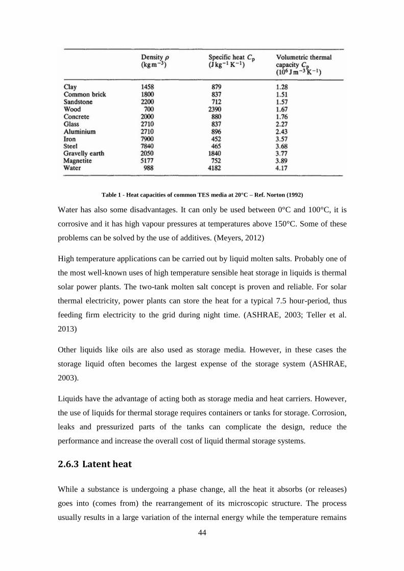
44
Table 1 - Heat capacities of common TES media at 20°C – Ref. Norton (1992)
Water has also some disadvantages. It can only be used between 0°C and 100°C, it is
corrosive and it has high vapour pressures at temperatures above 150°C. Some of these
problems can be solved by the use of additives. (Meyers, 2012)
High temperature applications can be carried out by liquid molten salts. Probably one of
the most well-known uses of high temperature sensible heat storage in liquids is thermal
solar power plants. The two-tank molten salt concept is proven and reliable. For solar
thermal electricity, power plants can store the heat for a typical 7.5 hour-period, thus
feeding firm electricity to the grid during night time. (ASHRAE, 2003; Teller et al.
2013)
Other liquids like oils are also used as storage media. However, in these cases the
storage liquid often becomes the largest expense of the storage system (ASHRAE,
2003).
Liquids have the advantage of acting both as storage media and heat carriers. However,
the use of liquids for thermal storage requires containers or tanks for storage. Corrosion,
leaks and pressurized parts of the tanks can complicate the design, reduce the
performance and increase the overall cost of liquid thermal storage systems.
2.6.3 Latent heat
While a substance is undergoing a phase change, all the heat it absorbs (or releases)
goes into (comes from) the rearrangement of its microscopic structure. The process
usually results in a large variation of the internal energy while the temperature remains

45
constant. This characteristic can be used for thermal storage. Since there is no change in
the temperature of the storage material, the heat appears to be latent.
Latent heat storage is a particularly attractive technique since it provides a high-energy
storage density and has the capacity to store and release heat at a constant temperature.
For example in the case of water, 80 times as much energy is required to melt 1 kg of
ice as to raise the temperature of 1 kg of water by 1°C. This means that a much smaller
weight and volume of material is needed to store a certain amount of energy (see Table
2). (Verma et al., 2006)
Substances and compounds used for latent heat storage are usually known as phase
change materials (PCM). Any kind of phase change process can be employed for heat
storage: solid-liquid, liquid-gas, solid-gas or even transitions between different
crystalline phases (solid-solid). Usually solid-liquid is the preferred choice since it does
not present a large variation in volume. Liquid-gas and solid-gas will not be described
in this section.
However the selection of a PCM should be determined by the following criteria
(Sharma et al., 2009):
Thermal properties - suitable phase-transition temperature, high latent heat of
transition, good heat transfer.
Physical properties - favourable phase equilibrium, high density, small volume
change, low vapour pressure.
Kinetic properties - no supercooling, sufficient crystallization rate.
Chemical properties - long-term chemical stability, compatibility with materials
of construction, no toxicity, no fire hazard.
Economics - abundant, available, cost effective.
The various PCMs are generally divided into three main groups: organic, inorganic and
eutectics (combinations and mixtures of both inorganic or organic PCMs).

46
Table 2 - PCM and sensible heat media properties. Ref: Farid et al. (2004)
Organic PCM
Organic compounds present several advantages such as non-corrosiveness, low or no
under cooling, chemical and thermal stability, ability of congruent melting, self-
nucleating properties and compatibility with conventional materials of construction.
Organic PCM can be further classified as paraffins and non-paraffins. (Verma et al.,
2006)
Paraffins
Paraffins consist of different chains of alkanes. The length of the chains determines
temperature and the latent heat of the phase change providing wide ranges of
operational temperatures. However, their high cost limits the use of paraffin to just
some technical grade ones. (Sharma et al., 2009; Farid et al., 2004)
The advantages of paraffin are: inert and stable below 500°C, small change in volume,
low vapour pressure, good nucleating properties, wide temperature ranges, relatively
high latent heat, non-toxic and non-corrosive over extended periods of storage. (Verma
et al., 2006; Sharma et al., 2009)
On the other hand, the main drawbacks are: low thermal conductivity, non-compatible
with plastic containers and moderately flammable. Nonetheless, some of these negative
characteristics can be partially palliated. (Sharma et al., 2009)
Non-paraffins
Non-paraffin organic are the most numerous PCM. Unlike paraffins, each material
presents different properties. However, overall non-paraffins show high heat of fusion,
47
inflammability, low thermal conductivity, toxicity and instability at high temperatures.
(Sharma et al., 2009)
Among non-paraffins, fatty acids present a potential for heat storage, especially for
space heating applications (Zalba et al., 2003; Farid et al., 2004). Fatty acids show good
no supercooling and latent heats comparable to paraffin’s. Their major drawback is their
cost, which is 2–2.5 times greater than that of technical grade paraffin’s (Sharma et al.,
2009).
Inorganic PCMs
Inorganic compounds include salt hydrates, salts, metals and alloys.
Salt hydrates are the most important group of PCMs. They present high latent heat of
fusion per unit volume, relatively high thermal conductivity (almost double of the
paraffin’s) and small volume changes on melting. They are compatible with plastics, not
very corrosive and only slightly toxic. Many salt hydrates are also fairly inexpensive.
(Sharma et al., 2009, Farid et al., 2004)
The major problem of salt hydrates is that most of them they melt incongruently. This
decreases the performance of the medium after every charge–discharge cycle. Another
shortcoming is that the rate of nucleation is generally very low leading to supercooling.
(Verma et al., 2006; Sharma et al., 2009; Farid et al., 2004)
Some of the features of metals are a low heat of fusion per unit weight, high heat of
fusion per unit volume, high thermal conductivity, low specific heat and relatively low
vapour pressure. Generally, the high weight of metals makes them unsuitable for
storage applications as PCMs. (Sharma et al., 2009)
2.6.4 Thermo-chemical storage
In thermo-chemical TES, heat is stored in the form of chemical compounds created by
an endothermic reaction and it is recovered again by recombining the compounds in an
exothermic reaction. The heat stored and released is equivalent to the heat (enthalpy) of
reaction. Sorption systems are also considered TES.
Thermochemical energy storage has a higher energy density than other types of TES,
allowing large quantities of energy to be stored in small volumes. Energy storage based

48
on chemical reactions is suitable for short and long-term applications but it is
particularly advantageous for long-term storage applications (even seasonal storage)
because the process involves almost no energy losses during the storing period as long
as the reactants are stored separately. Thus, with all these properties it is a promising
technology for residential and commercial buildings. (Abedin and Rosen, 2011; Teller
et al., 2013).
Suitable material for thermo-chemical storage should have large inner surfaces (i.e. high
porosity) and be hygroscopic. Zeolite (aluminium silicates) and silica gel (based on
silicon dioxide) are normally used. The operating range of zeolite is between 100 °C
and 300 °C, the operating range of silica gel between 40 °C and 100 °C. It has been
already proven, as an example, the capacity of zeolite in CHP biogas plants as a flexible
and long term TES material. (Teller et al., 2013; Velasco, 2012).
2.6.5 Applications
TES has a huge potential and innumerable applications. Wherever heat is being
produced, TES systems can store it so it can be used at some other time or even
transport it to some other place. Thus, TES has the ability of totally decouple heat
generation and consumption.
Within power generation, it has already be stated the important role that thermal storage
plays in thermosolar plants. However, it can be equally applied to fossil-fuel fired
generation, especially for CHP systems. Storing heat for its later use instead of releasing
it to the environment would increase the overall efficiency of power. The main reason
why TES is not widely applied yet within every means of energy production is the still
cheap price of fossil-fuels and the elevated cost of thermal storage technologies. The
increasing prices of fossil-fuels are likely to change this situation and make heat storage
worth. (Bailey, 2010)
TES also has a great potential coupled to solar thermal storage both at small scale for
domestic applications and at larger scales, even for seasonal storage. Thermal reservoirs
could be used to provide hot water or space heating and, at larger scales, they could also
be used for power generation by the use of organic Rankine cycles. (McMahan, 2006)

49
Besides power generation, distributed thermal storage in the form of domestic electric
storage heaters or water heaters can act as demand side management and help to
regulate the load in the grid. Flexible day-of-time tariffs would be necessary to make
this application profitable for end-users.
In addition to heat, thermal storage can also provide cooling services. Again, both small
and large scale applications are feasible including seasonal storage. As mentioned
before, ice and snow harvesting was probably the first application of TES and it’s a very
simple but good example of the “cold storage” capabilities of TES.
Related to the previous applications, PCM materials are very suitable for their
integration within the structure of buildings. They could store heat during the day to
avoid the use of heating systems during night and, the other way round, use the coolness
of the nights to avoid the use of cooling systems during the day. This application can
also be met by conventional sensible heat thermal masses but the constant temperature
output/input of PCMs makes them more appropriate and effective. (Richardson and
Woods, 2008)
Another interesting application can be the use of PCM as back-up systems for
protection of goods. They could be used within food, chemicals or medicines storage
and could provide the temperature necessary to preserve these goods in the event of a
temporary power outage. This option can complete or even substitute conventional and
expensive backup power generators. (Bailey, 2010)
These are just some of the most widely discussed applications in the literature.
However, as stated above, heat storage can be applied in a huge number of situations.
2.6.6 Conclusions
The following table summarizes the main characteristics of and differences between
TES systems.

50
Table 3- TES systems comparison. Ref. Abedin and Rosen (2011)
Sensible heat is an already mature technology and can be readily applicable to many
situations. Water is the most widely used storage medium. It makes storage simple,
easily available, hazardless and economic. However, the narrow temperature range of
water limits the number of possible applications. Solid materials are also an economic
and effective way of storing heat but have fewer applications, normally at small scale.
The high heat surface losses, the need of good insulation and the large size necessary to
make it efficient, are limit the potential of sensible heat storage. Nevertheless, it has
been already applied successfully in many areas for several years. Good examples are
domestic storage heaters and water cylinders. Besides some improvements in storage
materials and insulation, not much progress is expected in sensible heat storage.
PCM has higher heat storage capacity than sensible heat media and a wide operational
temperature range. It is also compact, has a very controllable output and a good overall
performance. It is a readily available technology but only for a limited number of

51
applications. Integration of PCMs in building construction materials or the replacement
of big water tanks by smaller PCM containers are good examples of its current
applicability.
The main drawbacks of latent storage are the high cost of PCMs, their low heat
conductivity and some undesirable chemical properties (like corrosion or chemical
instability). A lot of research on new materials suitable for heat storage is still needed to
make it an economic and effective technology. In fact, an enormous research work is
currently being done on PCMs, so they are likely to become the most important heat
storage technology in the near future.
Finally, thermo-chemical storage has the best thermal storage properties of the three
TES methods. It has very high energy densities, potential zero losses, transportability,
seasonal storage capabilities... However, it is not a readily available technology. It is
still being widely researched and, so far, it presents very high costs and puzzling
technical complexity. However, if the challenges associated to this technology were
overcome, the future potential of this technology would be enormous and could change
the current role of thermal storage making it a very effective energy storage method.
In conclusion, TES is not a very extended way of energy storage although it could be
very extensively applied since waste heat is a side product of many industrial processes,
especially power generation. Releasing this heat to the atmosphere instead of using it
limits the efficiency of these industrial processes to very low levels. One of the main
reasons for not using this waste heat is because it is not immediately necessary in the
place or at the time of production. TES can be used precisely to decouple generation and
use of heat and, thus, it has a large potential. Furthermore, the wide range of
technologies and temperature ranges that TES covers make the storage of thermal
technology suitable for almost any type of application.

52
2.7 Summary
The following table presents a brief comparison of the main characteristics of the
different storage technologies discussed in this section:
Technology Advantages Disadvantages Applications Power vs Energy
CAES High storage
capacity
(underground),
efficient partial-load
operation, flexibility
Low efficiency,
need of favourable
geological
formations, needs
natural gas
Energy arbitrage, renewable integration,
grid balancing, non-spinning reserves Best suited for
energy
applications
Flywheels High power
capacity, long life,
no environmental
impact
High self-discharge
rates, requires high
engineering
precision, high costs
Bridging of power disturbances, grid
support, renewable firming Best suited for
power
applications
PHS Mature, very high
storage capacity,
long life, flexibility
Low energy density,
need of favourable
geological
formations,
environmental
impact
Energy arbitrage, renewable integration,
grid balancing, non-spinning reserves Best suited for
energy
applications
Chemical
storage:
Hydrogen
and SNG
High storage
capabilities (TWh),
can be used directly
as fuel
Elevated cost, needs
complex
infrastructure, low
overall efficiency,
hydrogen storage
Energy arbitrage, seasonal storage,
ancillary services Best suited for
energy
applications
Lead-acid
batteries
Mature technology,
low cost, easy to
recycle
Low specific energy
and power, short
cycle life,
maintenance
Stand-alone systems, substation auxiliary
power, renewables firming
Well suited both
for energy and
power
applications
Ni-based
batteries
Mature, good energy
densities, long life,
flat discharge
voltage
Cost, toxicity Renewable integration, voltage support,
grid regulation
Li-ion
batteries
High efficiency,
high energy density,
huge potential
Cost, fragile, unsafe
at large scales
Renewable integration, voltage support,
grid regulation, T&D deferral
Sodium-
based
Long lifetime, good
discharge times, fast
High temperature,
insulation,
Power quality, grid stabilisation, time-
shifting, renewable integration

53
batteries response, large
potential
efficiency, fire
hazard
Flow
batteries
Sizeable capacity,
long life, short
response time
Low energy density,
efficiency, require
pumps, sensor…
Time-shifting, T&D deferral, renewable
integration, grid regulation
Supercapaci
tors
Durability, low
environmental
impact, high
efficiency. discharge
times from seconds
to hours
High self-discharge,
cost, low energy
density
Voltage support, power quality
Suitable for
power
applications
Sensible
thermal
storage
Mature, materials
readily available,
high temperature
range, low cost
High surface losses,
low energy densities
Efficiency improvement of industrial and
power generation processes with high
amounts of waste heat, solar thermal,
domestic hot water and space heating with
DSM and frequency response, industrial
and domestic cooling
Usually suitable
for thermal
energy storage
but, depending on
the material, it
can also provide
high heat power
outputs
PCM
thermal
storage
Constant
temperature
input/output, high
efficiency, small
losses, high energy
densities,
Materials not readily
available, limited
temperature range
for each material
cost
Potentially similar applications as sensible
heat storage but with reduced volumes
and effective building integration
Thermoche
mical
energy
storage
Very high energy
density, potentially
zero losses,
transportability
Still in the R&D
phases, cost,
reactions
Potentially similar applications as sensible
heat storage but with reduced volumes
and effective seasonal storage
Table 4 - Energy storage technologies comparison
It is remarkable that one of the simplest and most mature technologies with one of the
widest applicability ranges, sensible thermal storage, still has a high and unexploited
potential.
A very interesting application comes from the capabilities for DSM and frequency
response of domestic sensible TES. These are particularly well-suited for integrating
renewable generation in small isolated grids and can really make a difference in these
communities. Surprisingly, there is a lack of research and publications on this topic.
That is why the next part of this thesis gives an insight on how electrical sensible heat
storage can play a very important role in these scenarios and also provides an
experimental investigation of a storage heater.

54
3. Storage Heaters
3.1 Storage heater basics
3.1.1 Introduction
A storage heater is an electric heating device that stores thermal energy during low
electricity demand periods, usually at night, and releases the heat stored when required
during the day. They are also known as “night storage heaters”.
Heat is stored in a core formed of ceramic refractory bricks made of materials with a
high density and specific heat. The bricks have several grooves so that electric heating
elements can be embedded between them and heat them up. The core is well insulated
to prevent undesired energy losses, making the heat output as controllable as possible
and to avoid excessive temperatures in the outer surfaces of the heater.
Heat is usually released from the heater by radiation and convection processes in the
surface of the heater and/or by circulating air through the core of the heater.
Storage heaters were introduced in the domestic heating scheme back in the 1950s
(SotrageHeaters.com, 2013). Energy companies had a high base-load generation
capacity to meet the peak demand during the day. However, the demand was much
lower overnight resulting in an underutilised infrastructure and an inefficient operation2.
Electric heating was well regarded (just like everything that was electric) and very
common at that time. It was also, as it is today, very energy-consuming. The concepts of
storage heater and hot water cylinder (electric hot water tank boiler) were then
developed as a measure to make a better use of the energy resources at night by shifting
part of the energy demand from peak to off-peak times.
However, storage heaters and water cylinders could only report benefits to the end user
if off-peak energy was priced cheaper than on-peak electricity. Thus, the development
of storage heaters led to the introduction of off-peak tariffs. As an example, the British
economy 7 tariff was created in the late 70s for that purpose. These tariffs offered
2 As it has been stated before, base-load generation is cheap and efficient when running at maximum
capacity and the expenses of turning on or off large generators are large.
55
cheaper energy prices during the night so users could reduce their electricity bill by
using electrical appliances overnight. Obviously, off-peak tariffs were especially
attractive and designed for storage heaters and hot water cylinder users. Off-peak tariffs
require the installation of an extra electricity meter for off-peak electricity.
Generally, consumers have a strong opinion about storage heaters. There are people
who support them unconditionally while others are totally against any means of electric
heating. Nevertheless, just like any other technology, electric storage heaters present a
number of advantages and disadvantages when compared to other means of space
heating like gas boilers.
Advantages
The main advantages of storage heaters are:
They have a low capital cost
Their installation is very simple.
They require virtually no maintenance.
In combination with an off-peak tariff they are more economic than
conventional electric heating and the newest models claim to be comparable to
gas heating systems.
They are a good option for users out of the gas grid distribution area
100% of the energy consumed by the heater goes into the heating space.
They do not produce emissions at the place of use which can be a hazard (like
CO).
The can be CO2-free if the energy consumed is supplied renewables and nuclear
sources.
New models have the capability of being remotely controlled combined with
smart heaters and act, then, as demand side management.
Disadvantages
A large amount of heat is released by radiative and convective processes during
charging.
Also, some heat is released during the day by the same processes when not
needed.
56
They require planning the heating requirements for the following day. This can
be a problem during warm seasons when the temperature varies widely
depending on the time of the day or in case of the home owners being absent of
the building unexpectedly.
Closely related to the previous one, the controls can result complicated and, if
not operated correctly, over- or under-heating are likely to occur decreasing the
efficiency of the system.
Sizing of the device is also challenging and can lead to excess or lack of heating
too.
It is not an immediate source of heat.
If there is not an off-peak tariff available, their operation is very expensive and
less efficient than conventional electric heating
3.1.2 Structure, types and operation of storage heaters
Storage heaters possess a very simple structure. They basically consist of a metallic box
with a core formed by ceramic bricks. There are some heating elements embedded
between the bricks and a good insulation surrounds the core (see Figure 19 and Figure
20). There two possible core configurations available in the market: with horizontal
heating elements (Figure 20) and with vertical heating elements (Figure 19). These
configurations usually correspond to dynamic and static heaters respectively.
Static storage heaters
Static storage heaters are designed so that around 80%3 of the heat stored in the core is
released by radiative and convective processes occurring in the surface of the heater.
Another important characteristic is that the air is circulated in the core of the heater
solely by natural convection processes (see figure below).
3 This number is just an approximation based on different manufacturers’ claims. It varies from model to
model.

57
Figure 19 - Structure of a static storage heater - Source: http://www.heatersuk.com/g/48166/guide-to-storage-
heaters.html
Static storage heaters commonly include two controls: input and output.
The input control determines the amount of heat stored in the heater during the charging
period. It is usually a thermostatic control (Laverick, 2011) that simply sets the
maximum allowable core temperature. Logically, the higher the temperature the more
heat stored.
The output control regulates the air that enters (and leaves) the core of the heater by
adjusting the position of a number of dampers. The dampers are usually attached to
bimetal systems so that they are only opened when the core of the heater starts to cool
down and a ‘boost’ of the heat output is required. This system only controls around the
20% of the total heat released by the heater and it is usually not well understood by the
users. (Storage-heaters.com, 2013)
It is easy to see from the characteristics explained above that this kind of storage heaters
provide a gradual heat output throughout the day that is not very controllable. Thus,
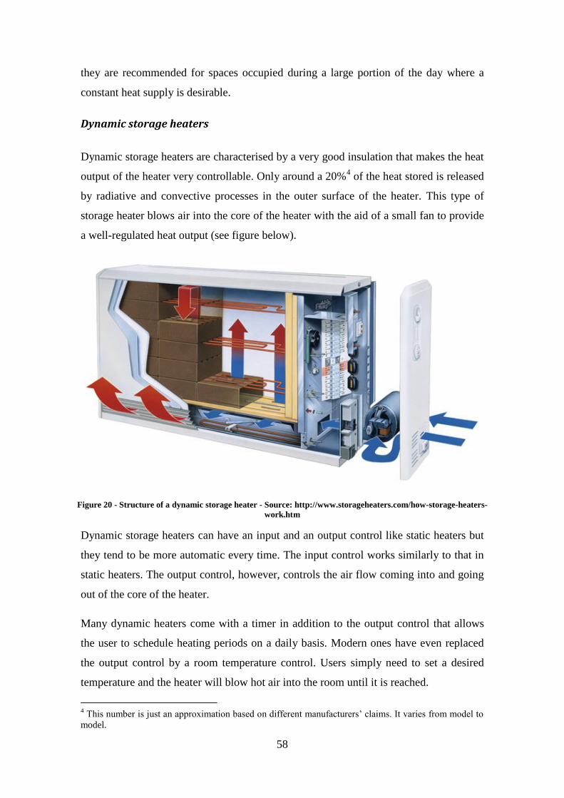
58
they are recommended for spaces occupied during a large portion of the day where a
constant heat supply is desirable.
Dynamic storage heaters
Dynamic storage heaters are characterised by a very good insulation that makes the heat
output of the heater very controllable. Only around a 20%4 of the heat stored is released
by radiative and convective processes in the outer surface of the heater. This type of
storage heater blows air into the core of the heater with the aid of a small fan to provide
a well-regulated heat output (see figure below).
Figure 20 - Structure of a dynamic storage heater - Source: http://www.storageheaters.com/how-storage-heaters-
work.htm
Dynamic storage heaters can have an input and an output control like static heaters but
they tend to be more automatic every time. The input control works similarly to that in
static heaters. The output control, however, controls the air flow coming into and going
out of the core of the heater.
Many dynamic heaters come with a timer in addition to the output control that allows
the user to schedule heating periods on a daily basis. Modern ones have even replaced
the output control by a room temperature control. Users simply need to set a desired
temperature and the heater will blow hot air into the room until it is reached.
4 This number is just an approximation based on different manufacturers’ claims. It varies from model to
model.

59
The current tendency in dynamic storage heaters is to eliminate the input control and
replace it by an automatic system. Modern heaters usually include a small built-in
computer that estimates the heating requirements of the following day based on weather
and usage patterns using a self-learning algorithm that charges the heater accordingly.
State-of-the-art dynamic heaters can also include a communication link system to allow
remote control from the grid utility suppliers. This way, the storage heater can help to
regulate the load in the grid acting as demand side management.
Finally, these heaters usually include a convector powered by a ‘boost element’ to
provide on-peak extra heating in case the stored heat is not enough to meet the heating
requirements.
Typical heat output profile
The following figure compares the typical heat output profiles from a static and a
dynamic storage heater:
Figure 21 - Static vs dynamic storage heater. Source: Heat Book Dimplex
http://www.dimplex.co.uk/assets/kb/brochure/0/Heat_Book.pdf
Their high controllability and reduced losses make dynamic heaters a more efficient and
effective way of providing space heating. The difference is height between the curves
gives an idea of the possible energy savings that a dynamic heater can provide
compared to static models. However, as stated before, static storage heaters may
provide adequate space heating in specific situations.

60
3.2 Storage heaters as demand side management
(DSM)
3.2.1 Demand side management
Definition and basics
Qureshi et al. (2011) define demand side management as “the planning,
implementation, and monitoring of distribution network utility activities designed to
influence customer use of electricity in ways that will produce desired changes in the
load shape, i.e. changes in the time pattern and magnitude of the network load.”
Put in simple terms, demand side management is the adjustment of consumer’s
electricity demand for the benefit of the grid. This can be performed manually by the
customer or automatically by the utility operator and can serve to accommodate an
excess of supply by increasing the load on the system or, contrarily, to avoid further
problems in case of a supply shortage by decreasing the demand.
As discussed in previous sections, the grid needs to provide a safe and reliable service
in every situation. In order to do that, power generation and distribution infrastructures
are designed to accommodate peak and not average demand. This way, it is ensured that
there is enough generation and transmission capacity installed to deal with unpredicted
deficits in the energy supply or sudden increases in the demand.
Historically, a capacity margin of around 20% was considered sufficient to provide
adequate security levels. Nevertheless, given the typical demand throughout a year, the
average utilisation of the global generation and transmission capacity is near 50%
(Strbac, 2008). Furthermore, it has already been discussed that the generation reserves
are mostly provided by inefficient partially-loaded generators and that the upgrading of
T&D lines is highly expensive.
Hence, a considerable fraction of the overall system capacity is underutilised because it
is necessary to accommodate the fluctuations of the energy demand (and variable
supply). The high-level objective of DSM is to flatten the load over time by “shaving
the peaks” and “filling the troughs” or, in other words: to transfer as much of the
flexible demand as possible away from peak time into periods of lower activity. The

61
main objectives of DSM are summarized in the figure below and their fulfilment would
result in a much more efficient system that would make feasible to downscale the
existing infrastructure without negative impacts on the power consumption. (Saffre and
Gedge, 2010)
Figure 22 - Main objectives of DSM - Ref. Qureshi et al. (2011)
In order to be beneficial for the end user, DSM has to be combined with dynamic
electricity prices that vary accordingly to the expected demand and supply. Nowadays,
only very basic day-night tariffs are available for the average customer. However, DSM
needs real-time reactive pricing mechanisms to be effective for the regulation of the
grid.
Currently, large industrial customers already curtail their demand when the frequency
drops below a certain value after a power loss in a generator or a similar event. They
usually obtain economic benefits from it. As an example, in the UK aluminium smelters
take part in this activity. Besides large industries, frequency could also be regulated by
time-flexible domestic electrical appliances. HVAC systems are good candidates for
this application. (Strbac, 2008)
Real-time reactive pricing mechanisms will be especially necessary with larger
integration of intermittent renewables. A communication infrastructure between the load
and the grid operators will be necessary to track supply and demand in real-time.
Depending on how well balanced the grid is at every time-step, prices would be updated
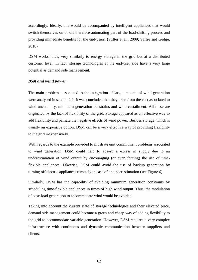
62
accordingly. Ideally, this would be accompanied by intelligent appliances that would
switch themselves on or off therefore automating part of the load-shifting process and
providing immediate benefits for the end-users. (Stifter et al., 2009; Saffre and Gedge,
2010)
DSM works, thus, very similarly to energy storage in the grid but at a distributed
customer level. In fact, storage technologies at the end-user side have a very large
potential as demand side management.
DSM and wind power
The main problems associated to the integration of large amounts of wind generation
were analysed in section 2.2. It was concluded that they arise from the cost associated to
wind uncertainty, minimum generation constrains and wind curtailment. All these are
originated by the lack of flexibility of the grid. Storage appeared as an effective way to
add flexibility and palliate the negative effects of wind power. Besides storage, which is
usually an expensive option, DSM can be a very effective way of providing flexibility
to the grid inexpensively.
With regards to the example provided to illustrate unit commitment problems associated
to wind generation, DSM could help to absorb a excess in supply due to an
underestimation of wind output by encouraging (or even forcing) the use of time-
flexible appliances. Likewise, DSM could avoid the use of backup generation by
turning off electric appliances remotely in case of an underestimation (see Figure 6).
Similarly, DSM has the capability of avoiding minimum generation constrains by
scheduling time-flexible appliances in times of high wind output. Thus, the modulation
of base-load generation to accommodate wind would be avoided.
Taking into account the current state of storage technologies and their elevated price,
demand side management could become a green and cheap way of adding flexibility to
the grid to accommodate variable generation. However, DSM requires a very complex
infrastructure with continuous and dynamic communication between suppliers and
clients.

63
Large vs. small scale DSM
The larger the network the more generation and T&D facilities, the more customers and,
consequently, the more complex the creation of a DSM infrastructure. This is the main
reason why DSM is not widely applied. The operational challenges, the necessary
technological infrastructure, the introduction of time-varying tariffs and the social
acceptance of remote control make large-scale DSM out-of-reach nowadays.
Nevertheless, DSM has a very important role to play in small isolated communities that
generate and administrate their own electricity, like islands. Due to the reduced size of
these grids, the implementation of a DSM infrastructure becomes more feasible. In
addition, these ‘experiments’ in small communities can provide very valuable
information for larger scale projects.
Many islands are not connected to the mainland electricity network and therefore need
to rely on their own power generation resources and manage their network. The Aegean
Islands in Greece, the King Island in Australia or the Shetlands and Eigg in Scotland are
good examples of this type of communities.
Just like in the mainland, islands need a reliable power generation source. This can only
be provided, at least currently, by fossil-fuel fired power stations. Islands usually install
diesel-fired power stations as their main energy supply. However, they result in
increasingly high running and maintenance costs. (Tsakiris, 2010; Hydro Tasmania,
2011; Eigg Electric, 2013; Pure energy centre, 2008).
Islands usually have greater renewable resources than the mainland. Wind is an
especially abundant resource in many of them. However, the capacity to deal with large
amounts of variable generation is very limited in small grids. The reduced number of
conventional generation makes the grid very inflexible. Therefore, these communities
cannot rely on wind or other intermittent renewables to obtain their electricity.
DSM has the potential to increase the amount of variable generation that can be
integrated in small energy networks. By monitoring the frequency of the grid, smart
appliances can turn on/off or increase/lower their consumption depending on the
availability of renewable resources. Furthermore, the conventional generation capacity
could be downsized since less generation reserves would be needed. This would reduce
the cost of energy production. Electric heating has a large potential as DSM.

64
3.2.2 Dynamic storage heaters capabilities for DSM
In addition to not being hooked into the mainland electric power network, small
communities are usually not connected to the gas grid either. Thus, electric space and
water heating usually represents a high percentage of the total energy consumption.
Storage heaters and hot water cylinders are the preferred means of electric heating since
they normally have low running costs if combined with night off-peak tariffs. Thus, hot
water cylinders and storage heaters are numerous and offer therefore a great potential
for DSM. Water cylinders will not be studied in this report although some of their
characteristics are very similar to those of storage heaters.
Modern dynamic storage heaters have a very good insulation and a highly controllable
output that makes them ideal candidates for DSM smart appliances. Two main types of
DSM can be identified for these devices:
- Charging scheduling:
It has been already stated that modern dynamic storage heaters have automated
charging controls that estimate the heating requirements for the following day
based on usage and weather patterns.
Utility providers can use the available wind speed and energy demand forecasts to
establish and schedule the optimum charging times for the heater.
In addition, the weather forecast information could also be used to estimate the
amount of heat necessary to meet the requirements of the household.
This information would be ideally sent to the heater on a daily basis although
updates throughout the day would be possible too.

65
Figure 23 - Storage heater as DSM. Charging scheduling
- Frequency response
Short-term demand side response can potentially be performed by storage heaters
too. By monitoring the frequency of the grid, heaters could detect imbalances in the
grid and automatically modify their energy consumption in real time.
Storage heaters usually have 3 heating elements and a boost function. By turning
on/off different numbers of heating elements, the energy consumption of the heater
can be modulated in real-time as well to provide frequency response.
The usage of storage heaters as DSM seems as a very effective way of regulating the
grid and making a better use of renewable resources in small communities. However,
storage heaters also present a number of issues that can affect their performance and
compromise their effectiveness as DSM:
Core temperature distribution and control– ceramic bricks used in the core of
the heaters exhibit low conductivities. This can lead to very uneven temperature
distributions in the core that can affect the amount of energy stored in the heater.
Furthermore, the level of charge is usually controlled by a single thermal sensor

66
located at the bottom of the core. This sensor reads the local temperature so it
may not give an accurate estimation of actual the level of stored energy. If only
some of the heating elements near the sensor are used to charge the heater up,
these problems are likely to be a larger concern.
Standing losses – passive heat losses reduce the amount of stored energy that
can be employed effectively.
Human factors – users usually do not usually have a deep understanding of the
operation of the heater. A wrong programming of the heater can result in
significant amounts of wasted energy (e.g. by opening a window due to an
excessive set temperature) and, thus, reduce the performance of heater.
The standard procedure to measure the performance of a storage heater is to use a
calorimeter room at a constant temperature. 24 hour tests with different charging and
discharging cycles are performed while energy is supplied to the room to keep a
constant temperature. Using a simple energy balance, the power supplied by the heater
can be estimated (NORDTEST, 1993)
This method can give a good idea of the heating capabilities and the heat losses in
standard test conditions. However, it does not provide any information about the
internal processes that take place inside the core of the heater and does not account for
real-life usage conditions. No relevant information has been found in the literature about
these issues so an experimental analysis of a dynamic storage heater is necessary to
better understand its behaviour and its real capabilities of storage heaters.
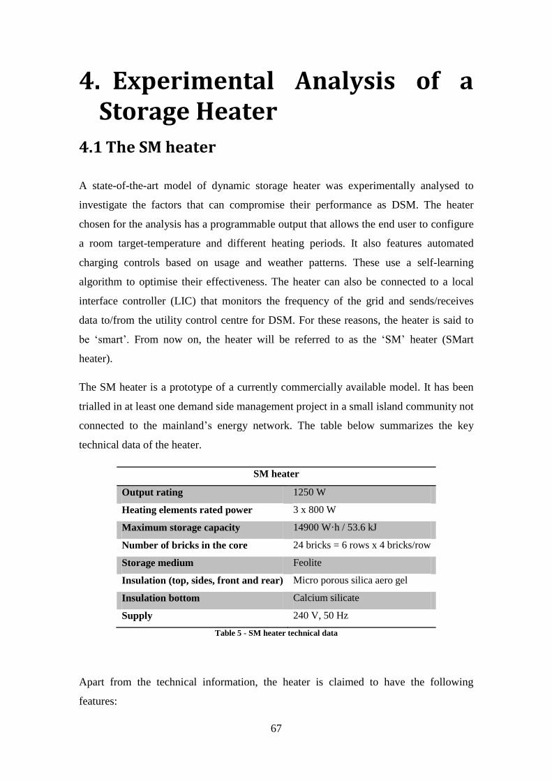
67
4. Experimental Analysis of a Storage Heater
4.1 The SM heater
A state-of-the-art model of dynamic storage heater was experimentally analysed to
investigate the factors that can compromise their performance as DSM. The heater
chosen for the analysis has a programmable output that allows the end user to configure
a room target-temperature and different heating periods. It also features automated
charging controls based on usage and weather patterns. These use a self-learning
algorithm to optimise their effectiveness. The heater can also be connected to a local
interface controller (LIC) that monitors the frequency of the grid and sends/receives
data to/from the utility control centre for DSM. For these reasons, the heater is said to
be ‘smart’. From now on, the heater will be referred to as the ‘SM’ heater (SMart
heater).
The SM heater is a prototype of a currently commercially available model. It has been
trialled in at least one demand side management project in a small island community not
connected to the mainland’s energy network. The table below summarizes the key
technical data of the heater.
SM heater
Output rating 1250 W
Heating elements rated power 3 x 800 W
Maximum storage capacity 14900 W·h / 53.6 kJ
Number of bricks in the core 24 bricks = 6 rows x 4 bricks/row
Storage medium Feolite
Insulation (top, sides, front and rear) Micro porous silica aero gel
Insulation bottom Calcium silicate
Supply 240 V, 50 Hz
Table 5 - SM heater technical data
Apart from the technical information, the heater is claimed to have the following
features:

68
A highly insulated storage core with very limited standing losses during non-
heating periods.
An energy efficient heat output that gives an accurate control of time and
temperature.
A simple user interface for setting comfort temperature and programming
heating periods.
An electronic control fully compatible with the distribution network operator
(DNO) interface, that provides:
o A communications link to utility for charging scheduling and frequency
response.
o Mains frequency monitoring.
o Variable frequency response.
o Variable input power of 0%, 33%, 66% and 100%.
o Core temperature sensing and setting.
o Ambient and room temperature sensing and setting.
Finally, the structure and the main elements of the SM heater are presented in the figure
below:
Figure 24- SM heater structure and main elements
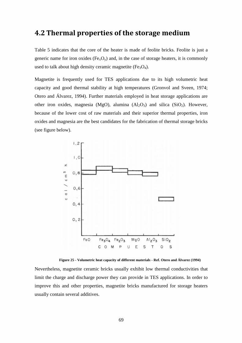
69
4.2 Thermal properties of the storage medium
Table 5 indicates that the core of the heater is made of feolite bricks. Feolite is just a
generic name for iron oxides (FexOy) and, in the case of storage heaters, it is commonly
used to talk about high density ceramic magnetite (Fe3O4).
Magnetite is frequently used for TES applications due to its high volumetric heat
capacity and good thermal stability at high temperatures (Gronvol and Sveen, 1974;
Otero and Álvarez, 1994). Further materials employed in heat storage applications are
other iron oxides, magnesia (MgO), alumina (Al2O3) and silica (SiO2). However,
because of the lower cost of raw materials and their superior thermal properties, iron
oxides and magnesia are the best candidates for the fabrication of thermal storage bricks
(see figure below).
Figure 25 - Volumetric heat capacity of different materials - Ref. Otero and Álvarez (1994)
Nevertheless, magnetite ceramic bricks usually exhibit low thermal conductivities that
limit the charge and discharge power they can provide in TES applications. In order to
improve this and other properties, magnetite bricks manufactured for storage heaters
usually contain several additives.

70
There is a lack of publications about the composition and thermal properties of
magnetite bricks used in storage heaters due to the possible economic consequences this
could bring to manufacturers. Therefore, prior to other analyses, the thermal properties
of the bricks used in the SM heater were studied.
4.2.1 Experimental set-up
Three samples were cut from different bricks of the SM heater and analysed in the range
from 25°C to 660°C. This is the range that can be expected in normal operational
conditions. The equipment used in this analysis comprises:
A scale and a calliper to measure the mass, volume and density of the samples at
room temperature.
A Netzsch DIL 402 C dilatometer.
A Netzsch LFA 427 laser flash analyser.
The thermal properties investigated in this analysis are interrelated by the definition of
thermal diffusivity,
Equation 1 - Thermal diffusivity
where α represents the thermal diffusivity, k the thermal conductivity, ρ the density and
CP is the specific heat capacity.
The thermal diffusivity of the three samples was directly measured by means of laser
flash analysis using the LFA 427. The basics of the laser flash analysis method (based
on the operation of the LFA 427) are explained below:
A small flat sample of material (10 mm x 10 mm x 5 mm in this case) is introduced in a
furnace where it faces a pulsed laser (see Figure 27). The sample is then heated up to a
certain temperature. When it attains a stable temperature, the laser emits a pulse of
energy that is absorbed at the front face of the sample. This results in a homogeneous
surface heating. The relative temperature increase on the rear face of the sample is then
monitored and measured as a function of time by an IR detector. A typical heating
profile can be found in Figure 26. These data are used to compute the thermal

71
diffusivity of the sample using especial software. For adiabatic conditions, α can be
estimated by the following equation:
Equation 2 - LFA thermal diffusivity
where l is the sample thickness and t0.5 the time at 50% of the temperature increase in
the rear face of the sample. (NETZSCH, 2013)
Figure 26 - Temperature increase in the rear face of a sample in LFA. Source:
http://www.calce.umd.edu/TSFA/laser_flash/Results.pdf
The specific heat of the samples was also analysed by the LFA 427. To do so, the
device measures the final temperature of the sample under investigation after the laser
pulse has been absorbed and compares this value with a standard reference sample
(graphite in this case). The basic concept behind this method is the following:
( ) ( ) ( ) ( )
Equation 3 - Cp estimation by comparison with standard reference sample.

72
Figure 27 - LFA 427 structure. Ref. NETZSCH (2013)
The density of one of the samples was measured at room temperature by estimating its
volume and weighting its mass. Then, its thermal expansion was analysed using the DIL
402 C dilatometer.
Finally, the results were combined via Equation 1 to work out the thermal conductivity
of the samples.
Three individual measures were taken per temperature point. The LFA method is
claimed to be have an accuracy of less than 4% for thermal diffusivity, heat capacity
and conductivity. In addition, the random uncertainty (reproducibility/precision)
amounts to 1–2% with three individual measurements taken per temperature point.
(Müller, n.d.)

73
4.2.2 Results
The results presented in this section are separated into a comparison and an average of
the three samples. The data shown for individual samples represent the mean value of
the three measurements taken per temperature point. Since the LFA method is very
precise (see above), the standard deviation is not significant in this case. However, the
average of the three samples accounts for the nine measurements taken per temperature
point (three per sample). The repeatability of LFA and the differences between samples
are both taken into account in the standard deviation which is represented as error bars.
Density
Graph 1 shows a very linear relation between density and temperature. The values of the
density of the sample at 25°C and 660°C differ roughly a 2%. Thus, it can be concluded
that the magnetite used in the SM heater presents excellent thermo-mechanical
properties within the studied temperature range.
These results are similar to other studies found in the literature. Densities from 3.6 to
4.0 g/cm3 are expected in the production of magnetite ceramic bricks and the rated
density of TAO-35 feolite bricks is 3.5 g/cm3 (Otero and Álvarez, 1994; Samot, n.d.).
Graph 1 - Density of magnetite used in the SM heater

74
Thermal diffusivity
The three samples exhibit slightly different results but a very similar variation of their
thermal diffusivity with temperature (see Graph 2 below). It is challenging to cut
identical samples of such a reduced size (10 mm x 10 mm x 5 mm) from a fragile
material like ceramic magnetite resulting in different masses and sizes. This is the origin
of the slight dissimilarities presented by the results of the three samples.
Ceramic and stone materials typically present low thermal diffusivities (~1 mm/s2).
Diffusivity represents the thermal inertia of materials, i.e. the ‘resistance’ that they
oppose to a change in its temperature. The lower the value of the diffusivity, the larger
the thermal inertia.
Graph 2 (right) shows that the diffusivity of the samples decreases from around 1.4
mm2/s at room temperature down to 0.5 mm
2/s at 660°C. This means that the bricks will
present sharper temperature profiles at high temperatures and, therefore, the temperature
distribution inside the core of the heater will tend to be more inhomogeneous as well.
Graph 2 – Storage medium. Thermal diffusivity

75
Specific heat
Again, the three samples present different results and a similar variation profile.
However, this time sample 1 displays significantly higher results than the other two
samples. As stated in section 4.2.1, the LFA 427 estimates CP by comparing the final
temperature after the heating with a reference sample. Therefore, slight variations in the
mass of the samples result in differences in the final temperature of the samples that
originate the dissimilarities shown in the graph below.
The higher the heat capacity the larger the amount of energy stored for a constant
temperature increase (see Equation 1). Graph 3 shows that the average specific heat of
the samples increases from 1.07 J/g·K at room temperature up to 1.94 J/g·K. However,
it does not grow steadily and presents a small dip at 400°C.
Graph 3 – Storage medium. Specific heat
Gronvold and Sveen (1974) carried out an extensive analysis of the heat capacity of
synthetic magnetite and its ferrimagnetic phase transition back in 1974. The results of
their research are summarized in the figure below:

76
Figure 28 - Specific heat of synthetic magnetite. Source: Gronvold and Sveen (1974) [1 mol magnetite = 231.54 g]
The results obtained in the present analysis differ widely from the ones shown in the
figure above. It can be easily observed that the overall heat capacity obtained for the
samples is significantly higher and there is no trace of a phase transition.
In addition, Samot (n.d.) sates that the mean value for the heat capacity of feolite bricks
TAO-35 in the range 20°C -700°C is 0.94 J/g·K.
In this study, the mean value of CP can be easily estimated from the data provided in
Graph 3 as:
∫ ( )
∫ ( )
Equation 4 - Mean value of CP from Graph 3. [The integration was performed assuming linear variation of the
heat capacity between consecutive points of Graph 3]
It is therefore clear that the heat capacity of the magnetite used in the SM heater does
not behave like standard synthetic magnetite or commercial TAO-35 feolite and
presents a significantly higher heat capacity.
Finally, it is important to note that CP is roughly double at high than at low temperatures
and, thus, the storage capabilities of the SM heater are double too.
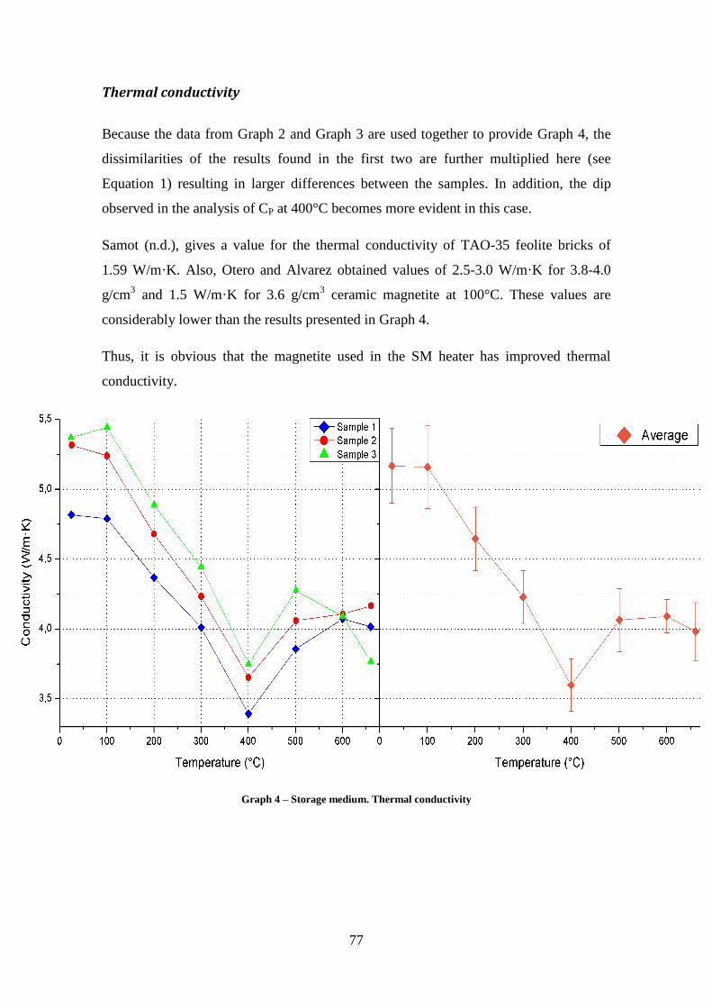
77
Thermal conductivity
Because the data from Graph 2 and Graph 3 are used together to provide Graph 4, the
dissimilarities of the results found in the first two are further multiplied here (see
Equation 1) resulting in larger differences between the samples. In addition, the dip
observed in the analysis of CP at 400°C becomes more evident in this case.
Samot (n.d.), gives a value for the thermal conductivity of TAO-35 feolite bricks of
1.59 W/m·K. Also, Otero and Alvarez obtained values of 2.5-3.0 W/m·K for 3.8-4.0
g/cm3 and 1.5 W/m·K for 3.6 g/cm
3 ceramic magnetite at 100°C. These values are
considerably lower than the results presented in Graph 4.
Thus, it is obvious that the magnetite used in the SM heater has improved thermal
conductivity.
Graph 4 – Storage medium. Thermal conductivity

78
4.2.3 Discussion and conclusions
The use of the word ‘feolite’ instead of magnetite in the specifications of the SM heater
was properly employed since the material analysed does not present any of the expected
properties of magnetite, apart from density.
In the manufacture of the bricks several grinding and heating processes are required to
obtain the final product. During these processes additives can be added to the raw
material in order to improve its consistency and its thermal properties. As stated in
sections 2.6.2 and 4.2 (see also Figure 25), MgO is also a very suitable material for
energy storage with a volumetric specific heat close to that of magnetite. Its main
advantage over the latter is its superior thermal conductivity (see figure below).
Therefore, the higher than expected thermal conductivity of the samples can be due to
MgO being used as an additive during the production of the bricks.
Figure 29 - Thermal conductivity of MgO. Source: http://nvlpubs.nist.gov/nistpubs/jres/103/4/j34sli.pdf
Likewise, the ferrimagnetic phase change of magnetite is not found explicitly in the
results. It has probably been shifted to higher temperatures or even smoothed out as a
consequence of the high temperature (above the critical temperature of magnetite)
processes during the manufacture of the bricks.
As stated above, CP represents the amount of energy that a material can store when its
temperature changes. At a microscopic level this is translated into vibration of

79
molecules in different modes. The root of the anomalous dip observed in the data at
400°C was investigated but no conclusions were attained. However, it can have its
origin in the unavailability of some of those vibrational modes at that specific
temperature. A deeper study of the specific heat should be performed around 400°C
using a better temperature resolution in order to determine the final cause of this
anomaly. Nevertheless, it does not affect significantly the storage capacity or
performance of the storage material.
With regard to the margin of error of the measurements, the standard deviation of the
results (around 5% for diffusivity and conductivity and 8% for specific heat) does not
account for the differences encountered compared to the values found in the literature.
Furthermore, a large portion of these uncertainties is due to the small differences in size
and mass of the samples more than to the accuracy and repeatability of LFA method.
In summary, the properties presented by the storage material of the SM heater can be
considered as very good for a ceramic storage medium. Thermal diffusivity and
conductivity indicate that the overall performance of the heater is likely to be better at
low temperatures with higher heat transfer rates and smoother temperatures profiles. On
the other hand, the storage capacity of the heater is potentially larger at high
temperatures. However, this higher capacity can be prevented by sharper temperature
profiles and less effective charging and discharging processes.
In order to better evaluate the overall performance of the heater and, particularly, its
effectiveness as DSM, it will be useful a direct study of the temperature distribution
inside its core.
4.3 Temperature distribution
The low thermal diffusivity and conductivity of the bricks of the SM heater may prevent
the heat to spread effectively from the heating elements to the rest of the core. In
addition, large heat losses may as well occur in some parts of the heater. All this can
cause some bricks or parts of them to be significantly colder or hotter than others.
A very inhomogeneous temperature distribution inside the core can significantly affect
the performance of a storage heater. If the temperature is not evenly distributed, the high
volumetric heat capacity of magnetite is under-used. This is especially true in the case

80
of heaters, like the SM heater, in which charge control is carried out by a single
thermosensor.
The temperature distribution inside the core of the heater during a typical charging cycle
was studied to analyse these issues.
4.3.1 Experimental set-up
As stated above, the SM heater determines the level of charge for the following day
from usage and weather patterns using smart controls and a self-learning algorithm.
However, a misconfiguration (or even damage) was caused to these controls prior to
this project and prevented their use in this study unfortunately.
In order to perform the experiments presented in this section, the internal controls of the
heater were bypassed. The three heating elements were connected directly to the mains
supply and three switches were installed to allow their individual operation.
Nevertheless, bypassing the internal controls of the heater resulted in some negative
consequences. The built-in temperature/charge control was lost. Thus, the heater had to
be operated manually without any knowledge about the maximum safely achievable
level of charge. In order to avoid possible hazards, the local core temperature was
maintained always below 650°C. However, this meant that the heater was used at
random conditions that did not correspond necessarily to standard operation settings or
rated storage capacity. In addition, the internal fan stopped working. Thus, it was not
possible to study the heat output and discharging processes.
The equipment provided for the realisation of the experiments was rather simple. It
basically consisted of 8 K-type thermocouples (TCs) and two USB interface to monitor
their readings using LabView. Also, a current clamp was supplied to monitor the current
going into the heater.
Due to the very reduced number of thermocouples, the heater had to be approximated to
a 2D system. The thermocouples were located as close as possible to the centre of the
bricks (red line in the figure below) and, thus, the temperature in this position was
assumed to represent the average transversal temperature.
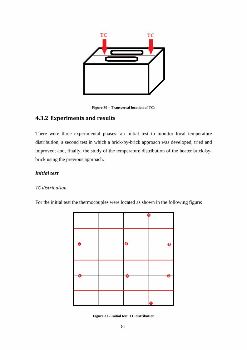
81
Figure 30 – Transversal location of TCs
4.3.2 Experiments and results
There were three experimental phases: an initial test to monitor local temperature
distribution, a second test in which a brick-by-brick approach was developed, tried and
improved; and, finally, the study of the temperature distribution of the heater brick-by-
brick using the previous approach.
Initial test
TC distribution
For the initial test the thermocouples were located as shown in the following figure:
Figure 31 - Initial test. TC distribution

82
The figure above represents the different bricks of the core of the heater with the
heating elements highlighted in red.
This distribution was chosen so that the thermocouples were as far as possible from the
heating elements to protect the sensors from excessive temperatures and to avoid
possible false readings caused by direct thermal radiation from the elements.
TC 1 was placed inside the bottom insulation, just where the original thermal sensor
used to control the temperature of the core of the SM heater is located. This
thermocouple was intended to be used as a reference temperature to compare the results
of different experiments.
Experimental conditions
The test was run for a 24-hour period. Prior to the start of the test the heater was
warmed up until TC1 was at around 100°C. Then, the heater was left stabilising for a
couple of hours. This warming up was performed to start the test with a stable
temperature distribution in approximately static conditions. When, TC6 and TC3 were
giving stable and similar readings of around 120°C the heating elements were turned on
for 6 hours. After the heating up period, the heater was left cooling down solely by
passive heat loss processes for near 18 hours.
Results
The results of this initial test are shown in the graph below:

83
Graph 5 – Initial test. TC temperature distribution.
It is easy to observe that some of the thermocouples give anomalous readings during the
experiment. The reason for this was discovered when the cover of the heater was
removed after the experiment. The coating of the thermocouple wire had melted down.
Some of the wires were in contact with others producing a mixed signal. It is difficult to
estimate the actual temperature at which this happened. However, it is clear that the
thermocouple wire provided for the project was not prepared for medium-high
temperature applications.
Besides these strange readings, Graph 5 shows an inhomogeneous temperature
distribution. The temperature is much higher in the centre of the heater than near the
sides. This difference exceeds 100°C at the end of the charging period.
It is interesting to note that TC2 and TC4 as well as TC5 and TC7 are found to give
similar readings throughout the experiment. This could mean that, although there is an
uneven distribution of temperatures, there may exist some symmetries in it.
Overall, the differences between the readings of the thermocouples increase during the
heating up period as the temperature rises and tend to be lower during the cooling down.

84
It can be found in the technical specifications of the heater states that the core has
reached its maximum storage capacity, Tcore = 600°C, when the thermal sensor located
at the bottom insulation gives a reading of 190°C. Nevertheless, Graph 5 indicates that
TC1 reached 190°C just after 2.5 hours of heating up. A typical charging period is much
longer than 2.5 hours so this result is largely inconsistent with the manufacturer’s
claims. The original thermosensor has a protective cover while the TC1 is completely
exposed. Thus, this is probably the origin of the discrepancy. Sadly, this means that the
results of the project cannot really be compared with nor calibrated against previous
studies and information from the manufacturer.
In summary, the temperature distribution in the core of the heater is very
inhomogeneous. The temperature in the centre and sides of the heater differs in more
than 100°C, roughly a 20%. However, the temperature distribution tends to homogenise
with time once the heating elements are turned off.
As a final remark, when the cover of the heater was removed at the end of the
experiments, besides the melted thermocouple wiring, the insulation panels of the heater
were found to be slightly burned. This probably means that, although the readings of the
thermocouples did not go beyond the maximum allowable core temperature (600°C),
some parts of the heater exceeded this value by far. This gives an idea of how local the
temperature can be and led to the design of the following test.
Second test – First brick-by-brick approach
To avoid the problems of the initial test, the thermocouples were covered in a high
temperature sleeving that can stand temperatures up to 650°C.
The previous results were useful to observe the inhomogeneities in the temperature
distribution at high-level. However, a more detailed study is needed to understand the
performance of the SM heater. Thus, it was decided to carry out a brick-by-brick
approach, i.e. to monitor every brick in an individual basis.
TC distribution
In order to carry out the brick-by-brick approach, the temperature of every brick was
monitored at four (three for the top bricks) different points (see Figure 32 and Figure
33). The temperature of the brick was then estimated averaging the four temperatures.

85
This is equivalent to a 2D integration assuming that the temperature varies linearly from
thermocouple to thermocouple.
An advantage of this method is that, inevitably, two of the thermocouples are placed
very near the heating elements and provide information about the maximum local core
temperature. That way, it is possible to avoid the excessive temperatures of the initial
test that led to the slight burning of the insulation panels.
Obviously several experiments are needed to monitor the temperature of the 24 bricks
that form the core of the SM heater using only eight thermocouples. In addition, the
initial and final conditions of the experiments need to be similar in order to join the data
from the different experiments together. TC1 was placed at the same location as in the
initial test for this purpose.
Only two experiments were performed in this second test. The first experiment
monitored the temperature of the first three bricks of the heater. The location of the
thermocouples can be found in the picture below:
Figure 32 – Second test. Experiment 1. TC distribution.
The second experiment monitored the temperature of the three following bricks:

86
Figure 33 - Second test. Experiment 2. TC distribution.
As seen in Figure 32 and Figure 33, two extra thermocouples, TC7/TC2 and TC8/TC3
are used as an extra reference to ensure similar conditions in both experiments.
However, for similar values of TC1, both experiments showed a mismatch in the
reading of the extra reference thermocouples (see graph below).
Graph 6 - Second test. Reference TCs comparison in experiments 1 and 2.

87
Although small, this gap represents a lack correlation between both experiments and
means that the initial conditions were different in each experiment and could not be
determined accurately from the reading of TC1. In order to make the results more
coherent, the data of the second experiment were time-shifted to match the first
experiment and the differences between the readings of T1, TC7/TC2 and TC8/TC3
were averaged.
Experiment conditions
The test was run for a 21.5 hours period. The core was first warmed up, like in the
previous test, until TC1 was giving a reading of around 150°C. Then the heater was left
stabilising for a couple of hours until the reading of TC1 was stable around 120°C. At
that point the heating elements were turned on for 5 hours and then the heater was left
cooling down solely by passive heat loss processes for 16 hours.
Results
The results of the two experiments are shown below:
Graph 7 - Second test. TC temperatures in experiments 1 (left) and 2 (right)
The graph above shows that the temperatures near the heating elements are much higher
than the others. In addition, just after the heating elements have been turned off, the
temperature of these thermocouples decreases very abruptly. This temperature drop is

88
generated by the sudden decrease of radiative heat arriving to the thermocouples as the
temperature of the heating elements decreases (Stefan-Boltzmann law E~T4). This
confirms the suspicions that led to the design of the initial test (see Figure 31) to avoid
false readings.
Beside these effects, experiment 1 shows a very diverse temperature distribution during
the whole cycle while in experiment 2, TC2, TC4, TC 6 and TC 8 (all of them located at
the right side of the heater, see Figure 32 and Figure 33) give similar readings.
Furthermore, all the thermocouples tend to reduce their differences during the cooling
period.
Some minor fluctuations of TC5 near the end of experiment 2 indicate that even with
the high temperature sleeving, the thermocouple wire is still likely to fail.
The results for the brick temperatures are now analysed. It should be remembered that
the data were modified to show coherence between experiments 1 and 2 as stated above.
Graph 8 - Second test. Brick temperature distribution

89
Although the temperature distribution is generally quite inhomogeneous locally, Graph
8 indicates that with a brick-by-brick approach the temperature distribution tends to be
more homogeneous for these six bricks.
Brick 1 shows a low temperature compared to the others. This is mainly due to the
readings of TC1. It is not in direct contact with brick 1 so its readings only account for
radiative and convective processes from the surface of the brick to the thermocouple
and, thus, tend to be lower.
Graph 8 also exhibits a sudden drop in the brick temperatures just after the heating
elements have been switched off. Although it is lower than for individual
thermocouples, it indicates that this first approach does not account for the expected
behaviour of the temperatures of the bricks. These should increase or remain a bit stable
just after the heating elements have been turned off since the latter are still hot and
provide energy for some time.
In conclusion, the brick-by-brick approach seems a reasonable way to study the
temperature distribution of the heater in detail. However, to monitor the temperature of
every brick using four thermocouples offers results deviated from the expected
behaviour. Thus, it should be avoided to place thermocouples near the heating elements
what, in fact, is quite challenging since a direct contact between the heating element and
the thermocouple wire would seriously damage the latter. In addition, too many
experiments are required using this approach and very little time was available for the
execution of the tests. Finally, it was quite challenging to perform the experiments in
the same exact initial condition using TC1 as a reference which is not in contact with
the bricks.
This is why only two experiments were performed using this method and a new
approach was developed.
A new approach
The results of the second test show that monitoring the temperature of the core brick by
brick provides a detailed view of the temperature distribution inside the core of the SM
heater. However, a simpler approach that requires fewer experiments and avoids placing
thermocouples near the heating elements is necessary.

90
Returning to Graph 7, it is easy to notice that the temperature of the thermocouples
located near the heating elements decreases very fast just after the latter are switched
off. A closer analysis reveals that their temperature does not only decrease but also
tends to reach a value slightly higher than the reading of the thermocouple located
directly below. As an example, on the left side of Graph 7, it can be observed that the
reading of TC8 decreases to values just above those of TC6 in less than 30 minutes.
In addition, Graph 5 and Graph 7 show that the higher the thermocouples are located
inside the heater the greater their readings.
Using these findings, a new approach was derived. Instead of placing four
thermocouples in every brick, the effective temperature near the heating elements is
now estimated as the average between the thermocouples located directly above and
below that position. The following figure illustrates the new approach.
Figure 34 – Finals tests. New approach for the estimation of the temperature of the bricks
In the figure above, thermocouples are located at positions 1, 2, 3 and 4. The
temperature in a and b would then be:
Ta and Tb computed this way, present values:
Lower than the real temperature while the heating elements are active
Similar to the temperature after the heating elements are switched off
Higher than the reading of the thermocouple located just below
Lower than the reading of the thermocouple located just above
This is in accordance with the observations stated above and, thus, can be used as an
effective temperature near the heating elements, i.e. as a temperature without the

91
distorting effects of the heating elements. However, it is important to stress that they do
not represent the real temperature at those locations. This is only an approximation in
order to estimate of the temperature of the bricks.
The following graph shows a comparison between the results of the second test using
the old approach and the new one:
Graph 9 – Final tests. Comparison between second test approach and the new one using the results from the
second test
The graph shows that the temperature evolution of the bricks remains very similar to the
second test but the abrupt drop after the deactivation of the heating elements is not
present. Furthermore, the temperature of the bricks keeps increasing after the heating
elements have been switched off. This is more like the expected behaviour. Therefore,

92
this new approach seems a better and more effective approximation to monitor the
temperature distribution inside the core of the heater.
Final test. Complete temperature distribution using a brick-by-brick approach.
TC distribution
5 experiments (plus some repetitions) were performed to obtain a complete picture of
the temperature distribution during a full charging cycle of the SM heater. The results
from all the experiments were joined together so that, overall, they are equivalent to a
single experiment using 18 thermocouples distributed in the following manner across
the core of the heater:
Figure 35 – Final tests. TC distribution
Experiment conditions
The tests were run for a 21.5 hours period. Prior to every test the heater was warmed up
until TC3 was giving a reading of around 120°C. Then the heater was left stabilising for
a couple of hours until the reading of TC3 was stable around 110°C. At that point the
heating elements were turned on for 5 hours and 40 minutes and then the heater was left
cooling down solely passive heat loss processes for 14 hours and 20 minutes.

93
TC results
Before investigating the temperature distribution in the core of the SM heater with the
new brick-by-brick approach, the results from individual thermocouples are analysed.
The following graph presents the readings of the thermocouples located at the sides of
the heater:
Graph 10 - Side thermocouples
The graph above shows very similar results for both sides of the heater indicating some
symmetry of the temperature distribution in the edges of the heater. The following
graph gathers together the readings of the thermocouples row by row:

94
Graph 11 – TC comparison between different rows
The graph above confirms that the temperature distribution in the SM heater presents
some symmetry. The lowest temperatures are found at the bottom side of the heater
(TC1-TC3-TC5). In contrast, the two middle rows exhibit the highest temperatures. The
top row (TC16-TC17-TC18) also presents high temperatures but slightly below the
latter. Within the rows, the temperature is observed to be much higher in the middle
than in the sides in all of them.
Brick-by-brick results
The temperatures of the bricks were estimated using the approach explained above. The
following graph presents the evolution of the temperature in every brick during the
whole cycle. The different graphs correspond to individual bricks and are located at the
position that they occupy inside the core of the heater (see Figure 35).

95
Graph 12 - Temperature evolution of every brick within the core of the SM heater

96
Although it is difficult to obtain a detailed picture of the instantaneous distribution of
temperature throughout the core from the graph above, it can be easily observed that the
temperatures in the sides are considerably lower than in the middle columns. In
addition, there is not an evident symmetry in the temperature distribution as in the case
of the analysis of the individual thermocouples presented above.
The following pages contain ‘snapshots’ of the temperature distribution in the core of
the SM heater taken every 30 minutes during the whole cycle. This way, it is easier to
picture the instantaneous distribution of temperatures. The higher temperatures are
symbolized with redder tonalities. It should be noted that all the values in the tables
below are given in °C.

97
t = 0 hours
122 125 123 120
120 125 122 116
118 125 121 114
116 124 120 112
113 120 117 111
108 113 112 108
t = 1.5 hours
210 248 244 211
208 243 234 201
208 247 231 198
212 251 235 202
209 246 233 203
198 231 224 200
t = 3 hours
300 359 353 297
301 354 341 290
304 360 337 288
309 365 343 293
302 354 336 292
284 329 318 284
t = 0.5 hours
148 168 166 147
142 158 155 138
140 159 151 136
144 164 155 139
143 163 155 139
137 155 151 138
t = 2 hours
241 288 283 241
240 282 272 231
242 287 268 229
246 292 273 233
241 284 269 234
228 266 257 230
t = 3.5 hours
329 394 388 326
332 389 375 319
336 396 371 318
340 401 377 324
332 388 369 321
312 359 347 311
t = 1 hour
178 207 204 179
174 201 194 170
174 204 192 167
178 209 196 170
176 205 195 171
168 194 189 170
t = 2.5 hours
272 325 320 270
272 320 308 262
274 326 304 260
278 330 310 265
273 321 305 264
257 299 289 258
t = 4 hours
358 428 421 354
362 423 408 348
367 431 404 348
371 435 410 353
361 421 401 350
339 389 376 336
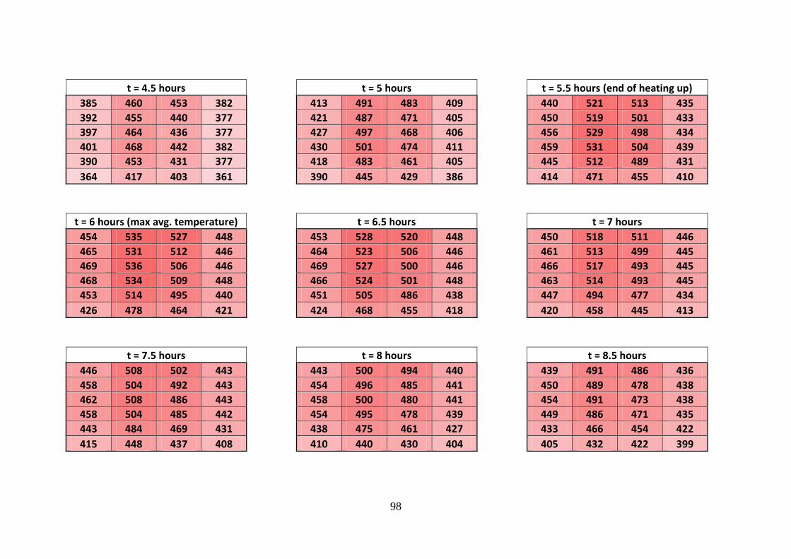
98
t = 4.5 hours
385 460 453 382
392 455 440 377
397 464 436 377
401 468 442 382
390 453 431 377
364 417 403 361
t = 6 hours (max avg. temperature)
454 535 527 448
465 531 512 446
469 536 506 446
468 534 509 448
453 514 495 440
426 478 464 421
t = 7.5 hours
446 508 502 443
458 504 492 443
462 508 486 443
458 504 485 442
443 484 469 431
415 448 437 408
t = 5 hours
413 491 483 409
421 487 471 405
427 497 468 406
430 501 474 411
418 483 461 405
390 445 429 386
t = 6.5 hours
453 528 520 448
464 523 506 446
469 527 500 446
466 524 501 448
451 505 486 438
424 468 455 418
t = 8 hours
443 500 494 440
454 496 485 441
458 500 480 441
454 495 478 439
438 475 461 427
410 440 430 404
t = 5.5 hours (end of heating up)
440 521 513 435
450 519 501 433
456 529 498 434
459 531 504 439
445 512 489 431
414 471 455 410
t = 7 hours
450 518 511 446
461 513 499 445
466 517 493 445
463 514 493 445
447 494 477 434
420 458 445 413
t = 8.5 hours
439 491 486 436
450 489 478 438
454 491 473 438
449 486 471 435
433 466 454 422
405 432 422 399

99
t = 9 hours
435 483 478 433
446 481 472 435
449 483 467 434
444 477 463 431
427 458 446 418
399 424 416 394
t = 10.5 hours
422 459 456 421
433 460 452 424
435 461 448 423
428 454 443 418
411 435 426 404
384 403 397 380
t = 12 hours
408 439 436 408
419 441 434 411
420 441 430 410
412 433 424 404
396 415 408 390
370 386 381 367
t = 9.5 hours
431 475 471 429
442 474 465 431
444 475 460 431
439 469 456 427
422 450 439 413
394 417 409 390
t = 11 hours
417 452 449 416
428 453 446 419
430 454 441 418
423 446 436 413
406 428 420 399
379 397 391 376
t = 12.5 hours
404 433 430 403
414 435 428 406
415 434 424 405
407 427 418 400
391 409 402 385
365 380 375 362
t = 10 hours
426 467 463 425
437 467 458 428
440 468 454 427
433 461 450 423
416 442 433 409
389 410 403 385
t = 11.5 hours
413 445 442 412
423 447 439 415
425 447 435 414
417 440 430 409
401 421 414 395
374 391 386 371
t = 13 hours
399 426 424 398
409 429 422 402
410 428 418 400
402 420 412 395
386 403 397 381
360 375 370 358

100
t = 13.5 hours
394 420 418 394
404 423 416 397
405 422 412 396
397 414 407 390
381 397 391 376
355 370 365 354
t = 15 hours
380 403 400 379
389 406 399 383
390 404 396 382
382 397 390 376
366 380 375 362
342 355 351 341
t = 16.5 hours
367 386 384 366
375 390 384 369
375 388 380 368
368 381 375 362
352 365 360 349
329 341 338 328
t = 14 hours
390 414 412 389
399 417 410 392
400 416 407 391
392 408 401 385
376 391 386 371
351 364 360 349
t = 15.5 hours
376 397 395 375
384 400 394 378
385 398 390 377
377 391 385 371
361 375 370 357
338 350 346 336
t = 17 hours
362 381 379 361
370 385 378 364
371 383 375 363
363 376 370 357
348 360 356 344
325 337 333 324
t = 14.5 hours
385 408 406 384
394 411 405 388
395 410 401 386
387 402 395 380
371 386 380 367
346 360 356 345
t =16 hours
371 391 389 370
379 395 389 373
380 393 385 372
372 386 380 366
357 370 365 353
333 345 342 332
t = 17.5 hours
358 376 374 357
366 379 373 360
366 378 370 359
358 370 365 353
343 355 351 340
321 332 329 320

101
t = 18 hours
353 371 369 352
361 374 368 355
361 372 365 354
354 365 360 348
339 351 346 336
317 328 325 316
t = 19.5 hours
340 356 354 339
347 360 354 342
347 358 351 341
340 351 346 335
326 337 333 323
305 316 313 305
t = 21 hours
328 343 341 326
335 346 341 329
335 344 338 328
328 338 333 323
314 324 320 311
294 304 301 294
t = 18.5 hours
349 366 364 348
356 369 364 351
357 367 361 349
349 361 355 344
335 346 342 331
313 324 321 312
t = 20 hours
336 352 350 335
343 355 349 338
343 353 346 336
336 346 341 331
322 333 329 319
302 312 309 301
t = 21.5 hours
324 338 336 322
330 341 336 325
330 339 333 324
323 333 328 319
310 320 316 307
291 300 298 290
t = 19 hours
345 361 359 343
352 364 359 346
352 362 356 345
345 356 350 339
330 341 337 327
309 320 317 309
t = 20.5 hours
332 347 345 330
339 350 345 333
339 348 342 332
332 342 337 327
318 328 324 315
298 308 305 297

102
It is easy to see from the tables above that during the heating up, the temporal evolution
of the temperature distribution looks very inhomogeneous. The middle columns heat up
much faster than the side columns and the difference between them increases rapidly
with the time. In addition, the middle-left column heats up faster than the middle-left
column and achieves greater maximum temperatures. On the other hand, the left side
column exhibits higher temperatures than the right side one. Thus, the temperature
distribution is not symmetric during the heating up since the right hand side of the
heater is appreciably colder than the left side.
In contrast, once the heating elements are switched off, the average temperature of the
core keeps increasing for almost 20 minutes (see also Graph 13). After this extra heating
period, the heater starts to lower its temperature. The hotter columns cool down faster.
Consequently, the temperature of the core tends to be more homogeneous.
Still, the tables presented above can be tedious to interpret due the high amount of data
they contain. Using very simple descriptive statistics techniques, the main features of
the temperature distribution are summarized in the two graphs below:
Graph 13 – Minimum, maximum and average core temperature

103
Graph 14 - Measurement of the dispersion of temperatures inside the core. Descriptive statistics
In Graph 14, the range indicates the difference between the maximum and minimum
temperatures inside the core (which are plotted in Graph 13). The range increases
rapidly and almost linearly during the heating up until reaching 120°C and the end of it.
Providing that the initial temperature of the core was around 120°C, the range shows a
maximum temperature difference of roughly a 30% between the coldest and the hottest
brick of the core. However, the range starts to go down just after the heating elements
are turned off decreasing rather fast until it reaches a value of approximately 50°C.
The interquartile range and the standard deviation represent the degree of dispersion of
the temperatures of the bricks. The larger they are, the more disperse the temperature
distribution is. Thus, Graph 14 confirms what was already described above when
describing the time evolution tables and the results in Graph 12: the temperature
distribution becomes more and more inhomogeneous during the heating up and starts to
homogenise just after the heating elements are switched off. From that point, the

104
homogenisation level keeps increasing although more and more slowly as the time
passes by.
Finally, the difference between the range and the interquartile range gives an idea of
how ‘extreme’ the minimum and maximum temperatures are with respect to the mean
value. Contrarily to the previous observations, this function achieves its maximum value
during the cooling down around two hours after the heating elements have been
switched off.
4.3.3 Storage capacity
Using the temperatures of the bricks, their masses and their heat capacity (see Graph 3)
it is possible to estimate the amount of heat stored in the core of the heater at each stage
of the cycle analysed above. In addition, the power input of the heater can be easily
estimated as well.
Finally, it is possible to perform a rough and simple approximation of the heat losses of
the SM heater during the heating up by comparing the power input and the energy
stored in the heater (losses = input – energy stored). It is also possible to estimate the
standing losses during the cooling down using this method at every point of the cycle
(losses = initial energy – final energy).
Power input
In order to monitor the power going into the heater during the charging process, two
different methods were used. On the one hand, a current clamp was used to monitor the
current passing through the heater directly. On the other hand, the resistance of the
heating elements and voltage were measured using a multimeter.
Both method showed rather stable power during the charging up of the heater and very
similar values to the rated power provided in the technical specifications of the heater.
The results are presented in the table below:
Resistance Total resistance Voltage Intensity Power Rated Power
67Ω + 68Ω + 69Ω
(in parallel) 22.7Ω 233 V (average)
10.33 A
(average)
2405 W
(average) 2400 W
Table 6 - Power, resistance, voltage and intensity of the SM heater

105
Thus, the total power input to the heater can be easily calculated as:
( )
Equation 5 - Total power input to the SM heater
Evaluation of the energy stored in the core of the SM heater
The energy stored in a single brick can be estimated by means of the following integral:
∫ ( )
Equation 6 - Estimation of the energy stored in a brick
If CP is constant during the temperature interval, then the equation above transforms
into the well-known expression E = m·CP·ΔT. In this analysis, CP is assumed to vary
linearly between consecutive points of Graph 3 in the form
( )
Equation 7 - Linear variation of CP (T)
The following parameters were found for the different steps of Graph 3:
Step a [·10-3
J/g·°C2] b [J/g·°C]
100°C - 200°C 1.18 1.172
200°C - 300°C 1.20 1.169
300°C - 400°C -0.19 1.585
400°C - 500°C 3.28 0.197
500°C - 600°C 0.160 1.037
Table 7 - Parameters of linear variation of CP
Combining Equation 6 and Equation 7 the following expression is obtained for the
determination of the energy stored in a brick in each temperature step:
∫ ( )
[ (
) ( )]
Equation 8 - Resolution of an integration step
Summing all the integration steps for every brick and, then, the results obtained for the
24 bricks that form the core of the SM heater, the energy contained in core is obtained.

106
Before performing these calculations, it should be stated that the average mass of the
bricks (using 6 bricks) was found to be 4.9 kg. Their original mass was 5 kg, but due to
their fragility and all the tests performed with the heater before and during this project,
some of them have lost part of their original mass.
Using the data of the heater at the initial conditions and its maximum temperature, the
following energies were calculated:
With these data, the total energy stored in the heater is found to be 17.8 kWh.
Obviously, there has been an overestimation of the energy stored in the heater since this
value is a 31% higher than the energy input to the heater.
A simpler but less ‘accurate’ method to estimate the energy stored, is to use the average
temperature of the heater and average CP. That way, the energy obtained would be:
Ti average Tf average Energy stored
118°C 480°C 17.6 kWh
Table 8 - Estimation of the stored energy using average temperatures
The value is very similar to the one obtained brick by brick and, thus, it is an
overestimation too.
The heater has been assumed to be a 2D system. It is likely that this is the main cause
for the overestimation of the energy stored inside the heater.
A last-minute experiment was conducted using the last four thermocouples that were
still working to monitor the temperature on the top of brick 19 (see Figure 35) at three
different transversal points. The figure below shows the locations of the thermocouples:

107
Figure 36 - 3D effect experiment. TC location
The results obtained in this last experiment are shown in the graph below:
Graph 15 - 3D effect experiment. Top of brick 19
Although a slight temperature difference is present between the three thermocouples, it
is evident that it is too small to account for the overestimation of the heat stored in the
core of the heater. The difference between the middle and the rear thermocouples
oscillated between 6.5% and 1.5 % with a 4% average. Compared to the 31% gap
between the energy input and the energy stored, this difference is insignificant.
It is important to notice that only two surfaces out of the six (plus the internal surfaces
of the air circulation holes) available in the bricks have been monitored throughout this
project. This was due to the very reduced number of thermocouples available for this
project. Therefore, further experiments to monitor the temperature of the bricks in every

108
surface are needed to address this issue. Unfortunately, they will have to be carried out
in following projects.
Another possible cause for the excessive value obtained of the energy stored inside the
heater could be an overestimation of CP. It has been shown in section 4.2.2 that the
average value obtained for CP is near a 70% higher than that of TAO-35 feolite.
This topic is further discussed in section 4.4.4.
Finally, since the results of the energy stored in the heater have been largely
overestimated using the brick-by-brick approach, a detailed study of the heat losses
using a comparison between the energy input and the energy stored is not possible.
4.3.4 Outer surface temperature
This section briefly presents the results obtained from a thermocouple placed at the
centre of the front panel of the heater. The following graph corresponds to the last-
minute experiment performed to assess the possible 3D effects in the heater and, thus, it
only covers 7 hours.
Graph 16 - Outer surface temperature
The graph above shows that the surface temperature increases steadily as the core of the
heater heats up. It reaches a maximum value of 57°C. As explained in section 4.3.1, the
controls were bypassed so it is not possible to know when the heater is at its maximum
rated capacity. Nevertheless, the experiments were designed to attain levels of charge

109
close to those in normal operation conditions. Therefore, the surface temperature is not
likely to be much hotter than 60°C at the heater’s rated storage capacity.
NSH (2013) states that exposed surfaces should not be hotter than 43°C to prevent
burns. Low surface temperature (LTS) heaters are designed to comply with that
indication. The SM heater is not an LTS heater and, therefore, needs to be used with
caution to avoid burning hazards. Nevertheless, its temperature is lower than that of
standard wall radiators. These usually reach temperatures of around 75°C and can
produce partial thickness burns in one second and full thickness burns in less than 10
seconds (Jaga, 2013; Ciphe, 2005).
4.4 Discussion
4.4.1 Remark about the validity of the experimental results
The experiments have shown that the brick-by-brick approach used to study the
temperature distribution in the core of the SM heater overestimates the average
temperature of the bricks. However, it still is a very reasonable and visual way of
monitoring the temperature distribution.
Likewise, it should be noted that this method was not designed to give accurate values
and was only adopted due to the limited number of thermocouples and overall resources
available for the experiments in this project.
Thus, in the following discussion, the reader should always bear in mind that the
approach is only valid to provide comparative values of the temperatures of the bricks
and not their real magnitude.
4.4.2 SM heater as a ‘night storage heater’
In this section, it is discussed how the performance of a storage heater may be affected
by its temperature distribution and heat losses when used as a night storage heater.
Some of the results from the experiments are used in the discussion.

110
Temperature distribution
As expected from the properties of ceramic magnetite, the temperature distribution has
been shown to be very inhomogeneous in all the tests performed on the heater.
However, if the SM heater is used simply as a night storage heater, i.e. charging it
solely during the night at off-peak time, the degree of inhomogeneity exhibited in the
experiments is not likely to affect the performance of the heater.
The SM heater automatically sets and controls the temperature of the core to meet the
energy requirements of the following day. Typically, the time necessary to charge the
heater, i.e. to achieve the set temperature, is significantly lower than the duration of the
off-peak charging period. Due to the standing heat losses of the heater, the heating
elements need to be switched on intermittently to maintain a constant temperature in the
core until the off-peak charging period finishes.
All the results obtained in the different experiments, especially those of Graph 14, show
that the temperature tends to homogenise rather fast just after the heating elements are
switched off due to the elevated temperature difference between different parts of the
heater. Thus, maintaining the temperature of the core at its maximum value during the
end of the charging period will tend to make the temperature distribution more
homogeneous.
This way, it is ensured that even if the local temperature around the thermosensor that
controls the charging process becomes eventually too high and the heating elements are
switched off too early, the inhomogeneities in the temperature distribution will tend to
be smoothed out. The heating elements will be turned on again and the rated level of
storage will probably be attained by the end of the charging period.
Therefore, the temperature distribution is likely to be less important if the SM heater is
used as a night storage heater. Probably, this is the reason why this topic cannot be
easily found in the literature. However, as it will be explained later on, the situation is
totally different when the heater is used as DSM.
Likewise, blowing air through the core of the heater to release the stored heat is also
likely to affect the temperature distribution of the core.

111
Since the internal controls of the heater had to be bypassed for the realisation of this
project, there were no automatic controls to regulate and maintain the temperature of the
core at a constant level nor the internal fan was working so these matters could not be
investigated in this project.
Heat losses
Heating up
Graph 16 gives a very approximate idea of how the temperature of the outer surface of
the heater changes during the heating up. It is clear that the larger the outside
temperature, the more radiative and convective losses from the heater to the room.
The convective losses have an approximately linear dependence with the surface
temperature while radiative losses typically increase with T4 so the latter will be the
dominant heat loss process.
Thus, the only idea that can be extracted from Graph 16 is that, logically, the heat losses
will increase during the charging up as the temperature of the core increases.
The standing losses that occur during the charging up of the heater are released to the
room during the night while the outside temperature is low and the dwelling is fully
occupied. Therefore, these heat losses are not wasted. They can be considered useful
heat since they help to maintain the temperature inside the house during night. This
results in less of the energy stored in the heater having to be released during the first
heating period in the morning (see Figure 21).
In addition, the losses will be greater with higher set core temperatures and these, in
turn, will set to higher values when the weather is colder so overheating problems are
not likely to happen.
Therefore, heat losses during the charging up of the heater should not be an important
concern in the SM heater if used as a night storage heater.
Cooling down
Graph 13 illustrates a good representation of the average loss of temperature in the core
of the heater during the cooling down. It shows that the temperature decreases very
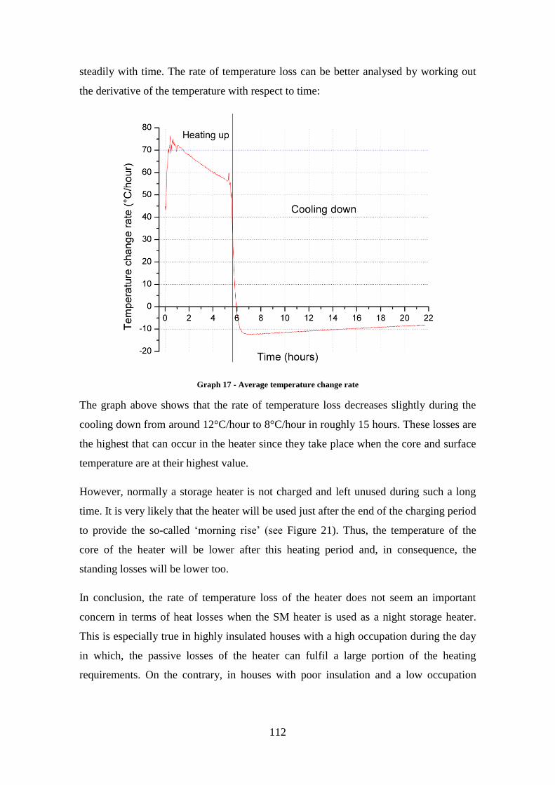
112
steadily with time. The rate of temperature loss can be better analysed by working out
the derivative of the temperature with respect to time:
Graph 17 - Average temperature change rate
The graph above shows that the rate of temperature loss decreases slightly during the
cooling down from around 12°C/hour to 8°C/hour in roughly 15 hours. These losses are
the highest that can occur in the heater since they take place when the core and surface
temperature are at their highest value.
However, normally a storage heater is not charged and left unused during such a long
time. It is very likely that the heater will be used just after the end of the charging period
to provide the so-called ‘morning rise’ (see Figure 21). Thus, the temperature of the
core of the heater will be lower after this heating period and, in consequence, the
standing losses will be lower too.
In conclusion, the rate of temperature loss of the heater does not seem an important
concern in terms of heat losses when the SM heater is used as a night storage heater.
This is especially true in highly insulated houses with a high occupation during the day
in which, the passive losses of the heater can fulfil a large portion of the heating
requirements. On the contrary, in houses with poor insulation and a low occupation
113
during the day in which the heater is left unused during long periods, the passive output
of the heater would be translated into lots of heat being wasted.
4.4.3 SM heater as demand side management
In this section, it is discussed how the performance of a storage heater may be affected
by its temperature distribution and heat losses when used as DSM. It is also explained
why the results from the experiments are not useful in this case and what type of
experiments should be done to address these issues.
Temperature distribution
Possible scenarios that may affect the performance of the SM heater
As explained above, the temperature distribution should not pose a problem if the heater
is used as a night storage heater because of the long charging period.
However, if used as demand side management the situation is totally different. Instead
of one long charging period overnight, there are several partial charges throughout the
day. Each charge has a set temperature associated and, therefore, a maximum allowable
core temperature.
If the heater is used as DSM to accommodate wind generation as discussed in section
3.2.2, the charging periods are usually in the scale from several minutes to a couple of
hours typical for the diurnal variation of the wind speed (Bentek Energy, 2010).
These kind of charging patterns were not studied in this project. Nevertheless, for the
results obtained for a full charging cycle, a very inhomogeneous temperature
distribution can be expected in short charging periods, with temperatures much higher
near the heating elements and in the centre of the heater (see Graph 7 and Graph 11).
In addition, the utility providers can programme one, two or the three heating elements
to turn on depending on the expected conditions of the grid. Only one or two heating
elements charging the heater may make the temperature much more unevenly
distributed than in the experiments performed during this project. Taking all this into
consideration, the following scenarios could occur:
114
If the local temperature near the thermosensor that controls the level of charge of the
heater increases faster than in other parts of the core, the heating elements may be
turned off too early. Since this sensor is located at the bottom of the SM heater, this
situation is more likely to occur when only the bottom heating element is used to charge
the heater. Contrarily to night storage heaters, there may not be enough time for this
local temperature to smooth out before the heating period ends. Thus, the heater would
not attain the expected level of charge.
This can lead to an early depletion of the heat stored and, consequently, to the activation
of the heating elements out of the predetermined heating periods, to avoid the core
temperature going below the minimum allowable.
On the other hand, if the local temperature near the sensor remains lower than in other
parts of the core, the opposite situation may take place resulting in too much energy
being charged. Furthermore, if during a heat output period the temperature near the
sensor is lower than it should be, the heating elements may need to be activated
although there may be enough energy stored in the heater to provide heating.
Finally, a very inhomogeneous temperature distribution during the release of heat may
cause the air to heat up at some points of the core and cool down at others decreasing its
effectiveness carrying the heat out of the heater.
Heat losses
The standing losses may be more significant for the performance of the heater as DSM
than they were for night storage heaters.
With partial charging cycles spread throughout the day, the temperature of the heater is
likely to be maintained at higher levels on average. Thus, the heat losses are potentially
greater.
If the heat losses occur in a highly insulated dwelling with a high level of occupancy
during the day, they will help to maintain the temperature of the house and contribute to
the fulfilment of the heating requirements. Nevertheless, if the heater is maintained at a
rather high temperature during a warm day it could lead to overheating.

115
On the other hand, in poorly insulated houses with long periods of no occupancy and no
usage of the heater, a higher average temperature means that more heat will be wasted.
Therefore, heat losses appear as a more important concern for DSM partial charging
cycles.
4.4.4 Energy stored and heat losses
The results of the brick-by-brick approach used to monitor the temperature of the core
of the heater during a charging cycle showed a value of 17.8 kWh for the energy stored
in the bricks (see section 4.3.3). This is an overestimation since the energy input to the
heater during the charging period was estimated to be a 31% lower.
According to the technical specifications of the SM heater, its storage capacity is rated
at 14.9 kWh (see Table 5). Unfortunately, the conditions under which this capacity was
estimated are not given.
However, the following assumption can be made: since the SM heater is designed to be
used mainly as a night storage heater using an off-peak tariff, it is likely that the rated
storage capacity corresponds to a full 7 hours overnight charging period. Thus, using the
rated charging power of the heater, it can be obtained that
2.4 kW · 7 h = 16.8 kWh
are delivered to the heater during the charging period. Using the method proposed in
section 4.3.3, it is possible to obtain a very rough approximation of the expected heat
losses that take place during the charging process of the heater as
16.8 kWh – 14.9 kWh = 1.9 kWh
Therefore, it can be concluded that the expected heat losses during the charging up of
the heater are in the range of 13% in normal operation conditions.
This result can be applied to the outcomes of the present project to provide a very crude
idea of the actual energy stored after the charging up period. Since the power input to
the heater has been estimated to be 13.4 kWh, the total energy would be around
13.4 kWh · 0.87 = 11.7 kWh.

116
This is a 21.5% less that the rated capacity of the SM heater. It is possible to estimate
the average CP that the storage medium should have in order to store 11.7 kWh with the
temperature difference obtained from the brick-by-brick approximation (see Table 8):
( )
Interestingly, this value is very similar to the specific heat of TAO-35 feolite (Samot,
n.d.) and the results by Gronvold and Sveen (1974). LFA is an accurate method and
three different samples were analysed giving similar results. In addition, the density and
thermal diffusivity obtained from the analysis of the samples present values within the
expected range. Conductivity, in contrast, exhibits improved characteristics but, as
explained in section 4.2.3, it is probably due to the presence of MgO in the storage
medium. Therefore, it is scarcely possible that a systematic error was committed during
the analysis that led to an overestimation of CP only without affecting other thermal
properties. The following discussion indicates that an overestimation of the temperature
of the core is a more probable cause.
In addition to the duration of the charging period, the initial conditions for the
estimation of the rated capacity are also unknown. Graph 5 and Graph 7 show, however,
that with heating times of 5-6 hours, very high local temperatures (more than 600°C) are
reached within the core. The manufacturer claims that, at full charge, the temperature of
the core should be around 600°C. It also needs to be taken into account, that the
manufacturer is likely to provide the value of the maximum storage capacity achievable
with the heater. Thus, for a 7 hour charging period, it seems reasonable that the storage
capacity has been worked out with heater starting the charging up at room temperature.
This way, local temperatures higher than 600°C are avoided and the value represents the
highest storage capacity.
Using these assumptions and the average heat capacity of the storage medium obtained
in section 4.2.2 (see Graph 3), it is possible to perform a rough investigation of the
maximum average core temperature expected at the rated heat capacity level:
( )

117
In contrast to this temperature, the average core temperature obtained from the
experimental data is 480°C. This is a 57% higher value than the one just obtained
above. The level of charge after the experiments carried out in this thesis is near the
rated storage capacity. Thus, it can be concluded that the overestimation of the core
temperature is approximately 50%.
As explained above, this overestimation arises from approximating the heater to a 2D
system. In addition, only the temperatures in the upper and lower surface of the bricks
were monitored. It is clear now that the temperature at these surfaces is much higher
than the average temperature of the bricks. Since the front and rear surfaces of the
bricks are in contact with the insulation panels their temperature is likely to be much
lower than in the upper and lower surfaces that are in contact with other hot bricks.
Therefore, the 3D characteristics of the temperature distribution need to be studied to
obtain a good approximation of the energy stored in the heater and the heat losses.
Sensors should be located in every external and internal surface of every brick to obtain
a 3D mapping of the temperature distribution. Unfortunately, this was not possible
during the project due to the limited time and equipment as mentioned before.
4.5 Conclusions and further work
4.5.1 Temperature distribution
The experimental results show clearly that the temperature distribution is very
inhomogeneous during the cycle studied. Since there are no data in the literature about
this topic, the information provided by this project is very valuable to understand the
internal behaviour of the SM heater.
In addition, the brick-by-brick approach introduced in this project appears as a useful
methodology to monitor the temperature distribution in high-detail using a small
number of sensors. However, as discussed above, the values that it provides are only
valid for temperature comparison between different parts of the bricks and do not
correspond the actual values of the average temperature of the bricks.
It should be noted that the heater needs to cool down completely to allow the
redistribution of the thermocouples between consecutive experiments and that one or

118
more reference temperatures are needed to gather the outcomes from the different
experiments together coherently. This evidently is very challenging and time-
consuming and, therefore, it is not an effective way of monitoring the temperature
distribution of the heater. It took more than eight experiments and around 25 days to
analyse a single charging cycle using this method. In addition, the temperature
distribution during discharging periods could not be studied either since the bypassing
of the controls made the internal fan to stop working.
In order to obtain a detailed study of the performance of the heater as DSM from its
temperature distribution, many different partial charging and discharging situations
have to be evaluated. This cannot be performed as several experiments are needed to
obtain a complete picture of the temperature distribution due to the difficulty of
replicating the exact same conditions in every partial experiment.
In addition, the performance of the heater as DSM will only be properly analysed if the
internal charging controls are employed. This was a very important limitation as well
for the possible outcomes of this project.
Therefore, the data provided by the experiments are obviously insufficient to evaluate
how the temperature distribution affects the performance of the heater as DSM. Thus,
the original aim of this project has been shown to be unreachable with the available
equipment and will need to be addressed in further studies. The results from the
experiments done in this project suggest that the temperature distribution is likely to
affect the performance of the heater as DSM as discussed above. Therefore, it is vital to
study this topic in detail.
For further work, the temperature distribution of the core should be monitored
completely and continuously using a very elevated number of sensors in a fixed
position. Using the internal control, different charging and discharging corresponding to
real life conditions should be simulated. Thus, dynamic information about the internal
state of the heater would be provided and would give results to better understand how
the SM heater behaves. From these data, it would be possible to optimise the charging
and discharging patterns and controls.

119
4.5.2 Energy stored and heat losses
Heat losses are usually monitored using a calorimeter room. This provides very accurate
results but they are only valid for the standard conditions of the experiment that do not
correspond to real-life conditions.
The method proposed in this project, i.e. to evaluate the heat losses from the amount of
energy stored in the heater at every moment, is a less accurate but very flexible method
that can be easily applied to monitor real-life standing losses. However, it has been
shown that it is necessary to have a detailed 3D map of the temperature distribution in
the core to provide a more or less accurate value of the energy stored and, thus, of the
losses.
Overall, heat losses are a very complex topic and depend on many different factors like
the location of the heater in the room, insulation of the building, usage patterns, open
doors and windows or occupancy. Thus, it very difficult to make generalisations about it
and could better be studied in further projects using computer modelling simulations.
The model proposed would provide simple experimental data that could be introduced
into the model.
4.5.3 Summary
In the early stages of the project, it seemed rather simple to monitor the temperatures
inside the core of the heater but soon after obtaining and analysing the first results it
came out that a very detailed study would be needed to obtain useful outcomes from the
experiments. The difficulty and technical complexity of the experimental part of this
project was highly underestimated.
Unfortunately, due to innumerable technical problems, by the time the author of this
thesis arrived to those conclusions, it was already too late to change the direction of the
experimental research to more achievable objectives. That is why the temperature
distribution was studied in detail although it was insufficient for evaluating the
performance of the heater as DSM.

120
However, the project has useful outputs like the methodology used for the study of the
temperature distribution using a limited number of thermocouples and the heat losses
evaluation from the amount of energy stored.
The concepts behind this project are of vital importance for the understanding of the
performance of storage heaters as DSM and highly advisable for further studies.
For future investigations it would be recommend to pay a great amount of attention
from the very early stages of the experiment to the high technical complexity associated
to the monitoring a very inhomogeneous temperature distribution, analyse in detail the
available resources and set achievable goals.
121
5. REFERENCES Abedin, AH and Rosen, MA. (2011). A Critical Review of Thermochemical Energy
Storage Systems . The Open Renewable Energy Journal. 4, 42-56.
Ackermann, T; Ancell, G; Borup, LD; Eriksen, PB; Ernst, B; Groome, F; Lange, M;
Möhrlen, C; Orths, AG; O’Sullivan, J; De la Torre, M. (2009). Where the Wind
Blows. IEEE power & energy magazine. 1540-7977
ASHRAE (2003). 2003 ASHRAE Applications Handbook.
Bailey, J. (2010). Modelling Phase Change Material Thermal Storage Systems.
Battery University. (2013). Alternate Battery Systems. Available:aaaaaaaaaaaaaaaaaaaa
http://batteryuniversity.com/learn/article/alternate_battery_systems.aaaaaaaaaaaaaaaa
Last accessed 16th Sep 2013.
Bentek Energy, LLC. (2010). Wind, Power and Unintended Consequences in the
Colorado Energy Market.
Brendan Kirby and Eric Hirst. (1997). ANCILLARY SERVICE DETAILS: VOLTAGE
CONTROL. OAK RIDGE NATIONAL LABORATORY. ORNL/CON-453
Carrington, D. (2013). Wind power capacity grew 20% globally in 2012, figures
show. Available: http://www.theguardian.com/environment/2013/feb/11/wind-power-
capacity-grew-2012. Last accessed 16th Sep 2013.
Chen, H; Zhang, X; Liu, J; Tan, C . (2013). Compressed Air Energy Storage. In: Energy
Storage - Technologies and Applications. Institute of Engineering Thermophysics,
Chinese Academy of Sciences, Beijing, 100190, China: INTECH.
Ciphe. (2005). Safe Surface Temperatures. Ciphe Data Byte.
D. S. Callaway and I. A. Hiskens. (2011). Achieving controllability of electric
loads. Proceedings of the IEEE. 99 (1), 184-199.
Dell, RM and Rand, DAJ. (2001). Energy storage — a key technology for global energy
sustainability. Journal of Power Sources. 100, 2-17.

122
Denholm, P and Sioshansi, R. (2009). The value of compressed air energy storage with
wind in transmission-constrained electric power systems. Energy Policy. 37 (8), 3149–
3158.
Denholm, P. (2012). Electric System Flexibility and Storage. Available:
http://www.nrel.gov/analysis/key_activities_integ_flex.html. Last accessed 16th Sep
2013.
Department of Energy (DOE). (1977). DOE Interagency Coordination Meeting on
Energy Storage, 1977, CONF 7709116.
Dincer, I and Rosen, M. (2011). In: Thermal energy storage : systems and applications.
John Wiley & Sons
Eames, P. (2013). The Future Role of Thermal Energy Storage in the UK Energy
System: Assessment of Technical Feasibility and Factors Influencing
Adoption. Available:
http://www.ukerc.ac.uk/support/RF3SmallThermalStorage&structure=Research.aaaa
Last accessed 16th Sep 2013.
Eckroad, S; Key, T.; Kamath, H. (2004). Assesment of Alternatives to Lead-Acid
Batteries for Substations. Bat-Con 2003.
Eigg Electric. (2013). Eigg Electric. Available: http://islandsgoinggreen.org/about/eigg-
electric/. Last accessed 16th Sep 2013.
energinet.dk. (2013). The Danish Market. Available:aaaaaaaaaaaaaaaaaaaaaaaaaaaaaaaa
http://www.windpower.org/en/knowledge/statistics/the_danish_market.html.aaaaaaaaa
Last accessed 16th Sep 2013.
EPRI-DOE. (2003). Handbook of Energy Storage for Transmission &Distribution
Applications. 1001834
Espinar, B and Mayer, D. (2011). The role of energy storage for mini-grid
stabilization. PVPS. IEA-PVPS T11-02:2011
European Commission. (2012). The EU climate and energy package.Available:
http://ec.europa.eu/clima/policies/package/index_en.htm. Last accessed 16th Sep 2013.

123
Eyer, J and Corey, G . (2010). Energy Storage for the Electricity Grid: Benefits and
Market Potential Assessment Guide. SANDIA REPORT. SAND2010-0815
Farid, MM; Khudhaira, AM; Razackb, SAK; Al-Hallajb, S. (2004). A review on phase
change energy storage: materials and applications.Energy Conversion and Management.
45 (9-10), 1597–1615.
Gronvold, F and Sveen, A. (1974). Heat capacity and thermodynamic properties of
synthetic magnetite from 300 to 1050K. Ferrimagnetic Transition and zero point
entropy. Journal of Chemical Thermodynamics. 6, 859-872.
Hadjipaschalis, I; Poullikkas, A; Efthimiou, V. (2009). Overview of current and future
energy storage technologies for electric power applications. Renewable and Sustainable
Energy Reviews. 13, 1513–1522.
Hydro Tasmania. (2011). Smart Grid. Available:aaaaaaaaaaaaaaaaaaaaaaaaaaaaaaaaaa
http://www.kingislandrenewableenergy.com.au/project-information/smart-grid.aaaaa
Last accessed 16th Sep 2013.
IEC. (2011). Electrical Energy Storage. White Paper.
Jaga. (2013). LST LOW SURFACE TEMPERATURE TECHNOLOGY. Available:
http://www.jaga.co.uk/technology/lst/. Last accessed 22th Sep 2013.
Karl Zach, Hans Auer, Günther Körbler, Georg Lettner. (2012). The Role of Bulk
Energy Storage in Facilitating Renewable Energy Expansion. stoRE.
Lannoye, E. (2012). Evaluation of Power System Flexibility. IEEE TRANSACTIONS
ON POWER SYSTEMS. 27, 922-93.
Laverick, R. (2011). Storage Heaters. Available: http://www.fastlec.co.uk/blog/?p=315.
Last accessed 16th Sep 2013.
Liu H and Jiang, J. (2007). Flywheel energy storage—An upswing technology for
energy sustainability. Energy and Buildings. 39, 599–604.
MCMAHAN, AC. (2006). Design & Optimization of Organic Rankine Cycle Solar-
Thermal Powerplants .

124
Meyers, R. (2012). Thermal Energy Storage. In: Encyclopedia of Sustainability Science
and Technology. Springer Science + Business Media.
Müller, WE. (n.d.). LFA – Laser flash apparatus. Available:aaaaaaaaaaaaaaaaaaaaa
http://www.dlr.de/wf/en/desktopdefault.aspx/tabid-2191/3208_read-4841/. Last
accessed 21st Sep 2013.
National Grid. (n.d.). Black Start. Available:aaaaaaaaaaaaaaaaaaaaaaaaaaaaaaaaaaaaaaa
http://www.nationalgrid.com/uk/electricity/balancing/services/balanceserv/systemsecuri
ty/blackstart/. Last accessed 22th Sep 2013.
National Grid. (2005). Understanding Electric Demand.
NETZSCH. (2013). Laser Flash Analysis. LFA 427 Technical Specification
NORDTEST. (1993). THERMAL STORAGE HEATERS: PERFORMANCE TEST.
Norton B., (1992) Solar Energy Thermal Technology, Springer-Verlag, Heidelburg,
Germany.
Nourai, A. (2007). Installation of the First Distributed Energy Storage System (DESS)
at American Electric Power (AEP). SANDIA REPORT. SAND2007-3580
Nourai, A.; Kogan, V.I.; Schafer, C.M.. (2008). Load Leveling Reduces T&D Line
Losses. IEEE Transactions on Power Delivery. 23 (4), 2168-2173.
Otero, JL and Álvarez, P. (1994). La magnetite en la fabricación de ladrillos para la
acumulación de calor. Rev Metal Madrid. 30 (3),
Paul Denholm, Erik Ela, Brendan Kirby, Michael Milligan. (2010). The Role of Energy
Storage with Renewable Electricity Generation. NREL.
Pradeep, K and Mohan, K . (2007). Alternative energy facilities based on site matching
and generation unit sizing for remote area power supply.Renewable Energy. 32, 1346-
1362.
Priyanka Samant. (2011). ENERGY STORAGE: APPLICATIONS AND DEVELOPING
REGULATION. Available:aaaaaaaaaaaaaaaaaaaa
http://www.dailyenergyreport.com/energy-storage-applications-and-developing-
regulation-2/. Last accessed 16th Sep 2013.

125
Pure energy centre. (2008). Shetland Energy SourceAnalysis. Available:
http://www.pureenergycentre.com/pureenergycentre/Energy%20Analysis%20Report.pd
f. Last accessed 16th Sep 2013.
Qureshi, WA; Nair, NKC; Farid, MM. (2011). Impact of energy storage in buildings on
electricity demand side management. Energy Conversion and Management. 52, 2110-
2120.
Rahul Walawalkar, Jay Apta, Rick Mancini. (2004). Economics of electric energy
storage for energy arbitrage and regulation in New York. Energy Policy. 35 (4), 2558–
2568.
Red Eléctrica de España. (2012). Síntesis. El Sistema Eléctrico Español.
Richardson MJ and Woods AW. (2008). An analysis of phase change material as
thermal mass. Available:aaaaaaaaaaaaaaaaaaaaaaaaaaaaaaaaaaaaaaaaaaaaaaaaaaaaaaaaa
http://rspa.royalsocietypublishing.org/content/464/2092/1029.full. Last accessed 16th
Sep 2013.
Richey, S. (2004). Flywheel Technology Helps Life Spring Eternal for Battery
Systems. Available: http://ecmweb.com/content/flywheel-technology-helps-life-spring-
eternal-battery-systems. Last accessed 16th Sep 2013.
Saffre, F and Gedge, R. (2010). Demand-Side Management for the Smart Grid . IEEE.
Samot. (n.d.). Thermal accumulation bricks (heavy) FEOLITE BRICKS. Available:
http://www.samot.co.rs/images/pdf/2%20alumino%20silicate%20%20sve%20strane%2
0refractry/Termal%20Acumulation%20Feolitebricks.PDF?Dir_level=2&Dir_Id=48.
Last accessed 16th Sep 2013.
Sandia Corporation. (2012). Glossary. Available:aaaaaaaaaaaaaaaaaaaaaaaaaaaaaaaa
http://www.energystorageexchange.org/application/glossary. Last accessed 16th Sep
2013.
Sayeef, S; Heslop, S; Cornforth, D; Moore, T; Percy, S; Ward, JK; Berry, A; Rowe, D.
(2012). Characterising the effect of high penetration solar intermittency on Australian
electricity networks. Australian Solar Institute.

126
Sharma, A; Tyagi, VV; Chen, CR; Buddhi, D. (2009). Review on thermal energy
storage with phase change materials and applications. Renewable and Sustainable
Energy Reviews. 13, 318–345.
Stifter, M et al.. (2009). Integration of Demand Side Management, Distributed
Generation, Renewable Energy Sources and Energy Storages. ieadsm.
StorageHeaters.com. (2013). History of storage heaters and the economy 7
tariff. Available: http://www.storageheaters.com/history-of-storage-heaters.htm. Last
accessed 16th Sep 2013.
Strbac, G. (2008). Demand side management: Benefits and challenges.Energy Policy.
36 (12), 4419–4426.
Strbac, G; Aunedi, M; Pudjianto, D; Djapic, P; Teng, F; Sturt, A; Jackravut, D; Sansom,
R; Yufit, V; Brandon, N. (2012). Strategic Assessment of the Role and Value of Energy
Storage Systems in the UK Low Carbon Energy Future. Imperial College London.
Teller, O. et al.. (2013). Joint EASE/EERA recommendations for a European Energy
Storage Technology Development Roadmap towards 2030.
Tsakiris, FR. (2010). Energy Development in the Non-Connected Islands of the Aegean
Sea . ORKUSTOFNUN.
Velasco, C. (2012). Compact and flexible thermal storage. Available:aaaaaaaaaaaaaaaaa
http://www.fraunhofer.de/en/press/research-news/2012/june/compact-and-flexible-
thermal-storage.html. Last accessed 16th Sep 2013.
Verma, P; Varun; Singal, SK. (2006). Review of mathematical modelling on latent heat
thermal energy storage systems using phase-change material. Renewable and
Sustainable Energy Reviews. 12, 999–1031.
Zalba, B; Marín, JM; Cabeza, LF; Mehling, H. (2003). Review on thermal energy
storage with phase change: materials, heat transfer analysis and applications. Applied
Thermal Engineering. 23, 251-283.