
An example of constraining well test interpretation with .... Well test Illumination.pdf · An...
24
An example of constraining well test interpretation with the help of seismic By Hamidreza Hamdi Patrick Corbett Andrew Curtis (Edinburgh Uni.) Colin MacBeth 1 “Joint Interpretation of Rapid 4D Seismic with Pressure Transient Analysis”, EAGE/SPE EUROPEC 2010
Transcript of An example of constraining well test interpretation with .... Well test Illumination.pdf · An...
An example of constraining well test interpretation with the help of seismic
ByHamidreza Hamdi
Patrick CorbettAndrew Curtis (Edinburgh Uni.)
Colin MacBeth
1
“Joint Interpretation of Rapid 4D Seismic with Pressure Transient Analysis”, EAGE/SPE EUROPEC 2010
Outline
• Overview of Well Testing– Information obtained from well test– Importance of Model recognition
• An integration example– Stratigraphic discontinuity detection (4D seismic)– Numerical well-test interpretation
• Deterministic approach• Inverse approach
• Conclusions
2
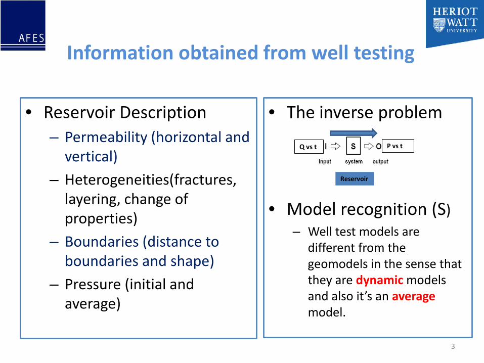
Information obtained from well testing
• Reservoir Description– Permeability (horizontal and
vertical)
– Heterogeneities(fractures, layering, change of properties)
– Boundaries (distance to boundaries and shape)
– Pressure (initial and average)
3
• The inverse problem
• Model recognition (S)– Well test models are
different from the geomodels in the sense that they are dynamic models and also it’s an averagemodel.
Q vs t
Reservoir
P vs t
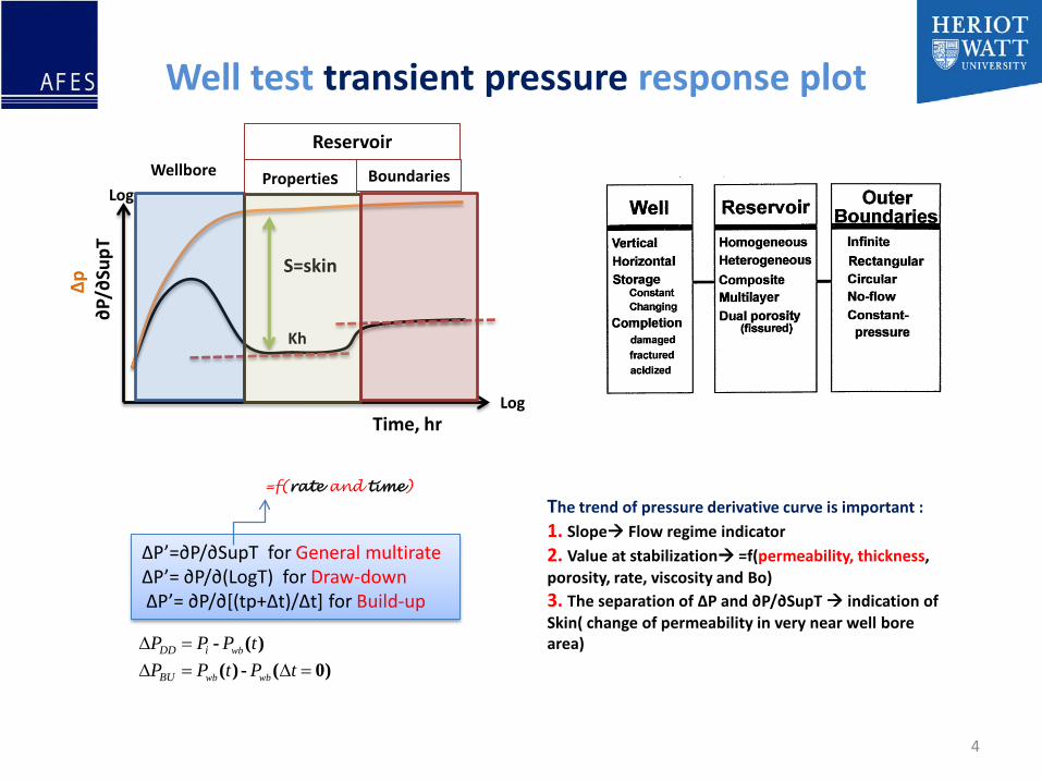
Well test transient pressure response plot
4
wb
wb wb
DD i
BU
P P P tP P t P t
∆ =∆ = ∆ =
- ( )( ) - ( 0)
∆P’=∂P/∂SupT for General multirate∆P’= ∂P/∂(LogT) for Draw-down∆P’= ∂P/∂[(tp+∆t)/∆t] for Build-up
∂P/∂
SupT
Time, hrLog
Log
Kh
∆p S=skin
Wellbore
Reservoir
Properties Boundaries
=f(rate and time)The trend of pressure derivative curve is important :1. Slope Flow regime indicator2. Value at stabilization =f(permeability, thickness, porosity, rate, viscosity and Bo)3. The separation of ∆P and ∂P/∂SupT indication of Skin( change of permeability in very near well bore area)
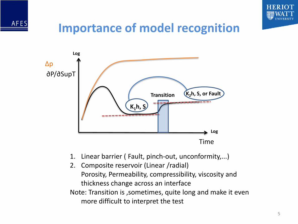
Importance of model recognition
5
∂P/∂SupT
Time
Log
Log
1. Linear barrier ( Fault, pinch-out, unconformity,...) 2. Composite reservoir (Linear /radial)
Porosity, Permeability, compressibility, viscosity and thickness change across an interface
Note: Transition is ,sometimes, quite long and make it even more difficult to interpret the test
Transition K2h, S, or Fault
K1h, S
∆p
outline
• Overview of Well Testing– Information obtained from well test– Uncertainty in model recognition
• An Integration Example– Stratigraphic discontinuity detection (4D seismic)– Numerical well-test Interpretation
• Deterministic approach• Inverse Approach
• Conclusions
6
7
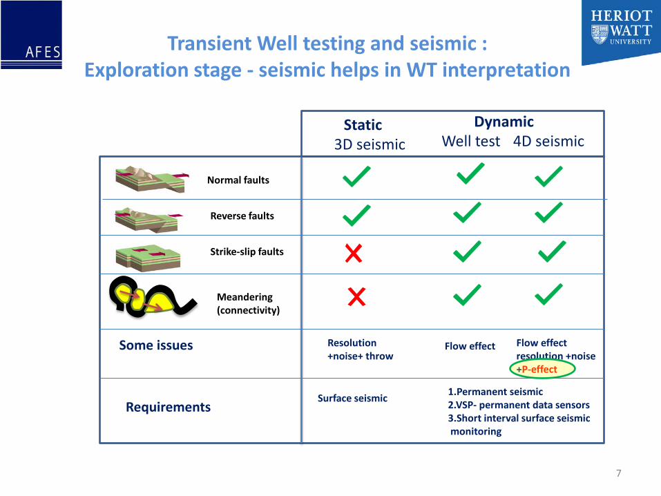
Static DynamicWell test 4D seismic3D seismic
Resolution +noise+ throw
Flow effect Flow effect resolution +noise +P-effect
Some issues
1.Permanent seismic2.VSP- permanent data sensors3.Short interval surface seismicmonitoring
Surface seismicRequirements
Normal faults
Reverse faults
Strike-slip faults
Meandering(connectivity)
Transient Well testing and seismic :Exploration stage - seismic helps in WT interpretation
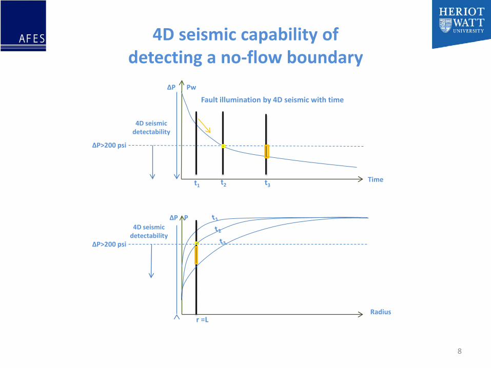
4D seismic capability of detecting a no-flow boundary
8
∆P Pw
4D seismic detectability
∆P>200 psi
Time
Radius
∆P4D seismic
detectability∆P>200 psi
P
Fault illumination by 4D seismic with time
t1 t2 t3
r =L
9
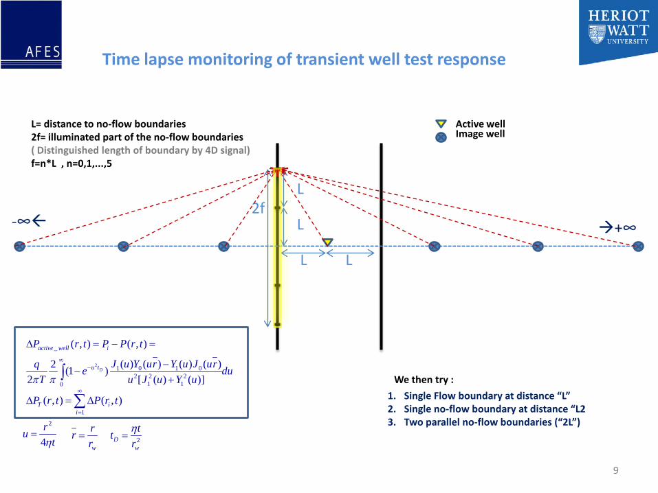
Time lapse monitoring of transient well test response
+∞-∞
L L
L
L2f
L= distance to no-flow boundaries2f= illuminated part of the no-flow boundaries( Distinguished length of boundary by 4D signal)f=n*L , n=0,1,...,5
Active wellImage well
2
_
1 0 1 02 2 2
1 10
( , ) ( , )
( ) ( ) ( ) ( )2 (1 )2 [ ( ) ( )]
D
active well i
u t
P r t P P r t
J u Y ur Y u J urq e duT u J u Y uπ π
∞−
∆ = − =
−−
+∫
1( , ) ( , )T i
iP r t P r t
∞
=
∆ = ∆∑
w
rrr
= 2Dw
ttrη
=2
4ru
tη=
1. Single Flow boundary at distance “L”2. Single no-flow boundary at distance “L23. Two parallel no-flow boundaries (“2L”)
We then try :
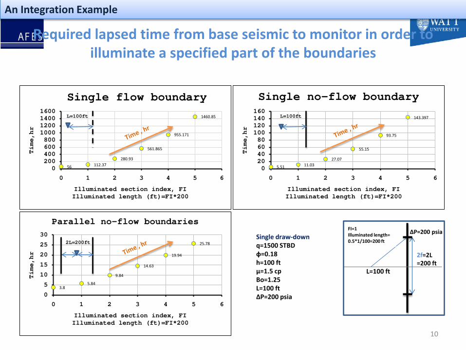
Required lapsed time from base seismic to monitor in order to illuminate a specified part of the boundaries
10
56 112.37280.93
561.865
955.171
1460.85
0200400600800
1000120014001600
0 1 2 3 4 5 6
Time,hr
Illuminated section index, FIIlluminated length (ft)=FI*200
Single flow boundaryL=100ft
5.51 11.0327.07
55.15
93.75
143.397
020406080
100120140160
0 1 2 3 4 5 6
Time,hr
Illuminated section index, FIIlluminated length (ft)=FI*200
Single no-flow boundary
L=100ft
3.85.84
9.84
14.63
19.94
25.78
0
5
10
15
20
25
30
0 1 2 3 4 5 6
Time,hr
Illuminated section index, FIIlluminated length (ft)=FI*200
Parallel no-flow boundaries
2L=200ftSingle draw-downq=1500 STBDф=0.18h=100 ftμ=1.5 cpBo=1.25L=100 ft∆P=200 psia
2f=2L =200 ft
L=100 ft
FI=1Illuminated length= 0.5*1/100=200 ft
An Integration Example
∆P=200 psia
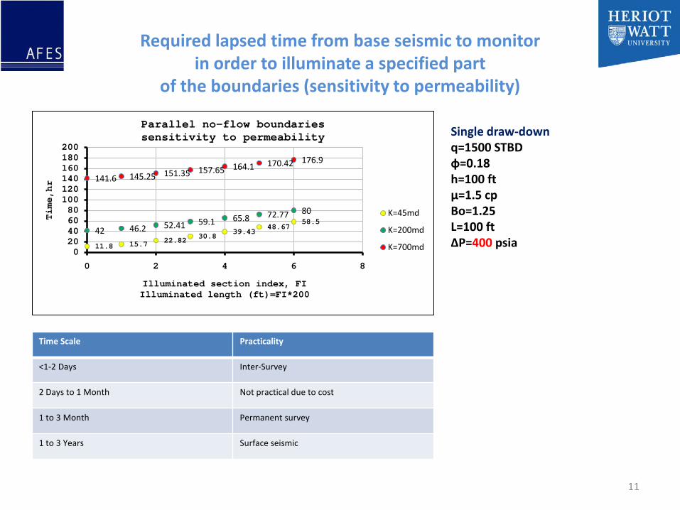
Required lapsed time from base seismic to monitor in order to illuminate a specified part
of the boundaries (sensitivity to permeability)
11
11.8 15.7 22.82 30.839.43
48.6758.5
42 46.2 52.41 59.1 65.8 72.77 80
141.6 145.25 151.35 157.65 164.1 170.42 176.9
020406080
100120140160180200
0 2 4 6 8
Time,hr
Illuminated section index, FIIlluminated length (ft)=FI*200
Parallel no-flow boundariessensitivity to permeability
K=45md
K=200md
K=700md
Single draw-downq=1500 STBDф=0.18h=100 ftμ=1.5 cpBo=1.25L=100 ft∆P=400 psia
Time Scale Practicality
<1-2 Days Inter-Survey
2 Days to 1 Month Not practical due to cost
1 to 3 Month Permanent survey
1 to 3 Years Surface seismic
Well testing and Seismic Example
• Seismic can help well test interpretation– Major Faults (3D Seismic)
– Sub-seismic faults (3D & 4D)
– Permeability baffles (4D)
• Numerical well test interpretation– Deterministic permeability profile+ seismic
– Inverse mobility and diffusivity map +seismic• Laplacian operator as a sectorization operator
12
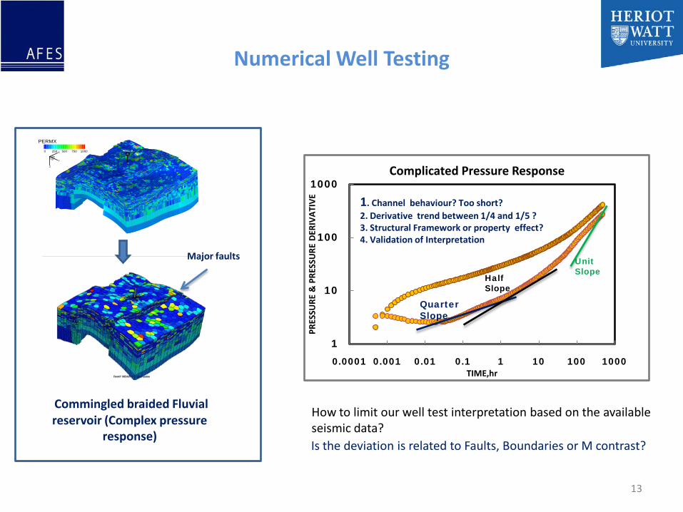
Numerical Well Testing
Is the deviation is related to Faults, Boundaries or M contrast?
Commingled braided Fluvial reservoir (Complex pressure
response)
How to limit our well test interpretation based on the available seismic data?
13
WELL-AX
Z
Y
0 250 500 750 1000
PERMX
Major faults
1
10
100
1000
0.0001 0.001 0.01 0.1 1 10 100 1000
PRES
SURE
& P
RESS
URE
DER
IVA
TIV
E
TIME,hr
Complicated Pressure Response
Quarter Slope
Half Slope
UnitSlope
1. Channel behaviour? Too short?2. Derivative trend between 1/4 and 1/5 ? 3. Structural Framework or property effect?4. Validation of Interpretation
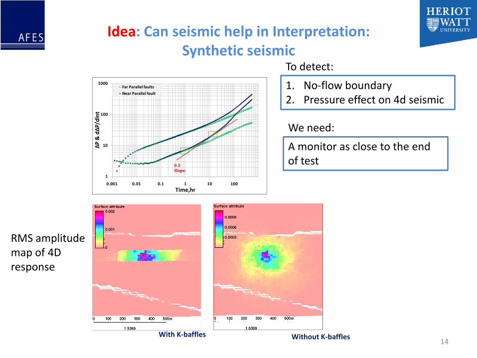
1
10
100
1000
0.001 0.01 0.1 1 10 100
∆P &
d∆P
/dln
t
Time,hr
Far Parallel faults
Near Parallel fault
0.5 Slope
Idea: Can seismic help in Interpretation: Synthetic seismic
14Without K-bafflesWith K-baffles
RMS amplitude map of 4D response
1. No-flow boundary2. Pressure effect on 4d seismic
A monitor as close to the end of test
To detect:
We need:
15
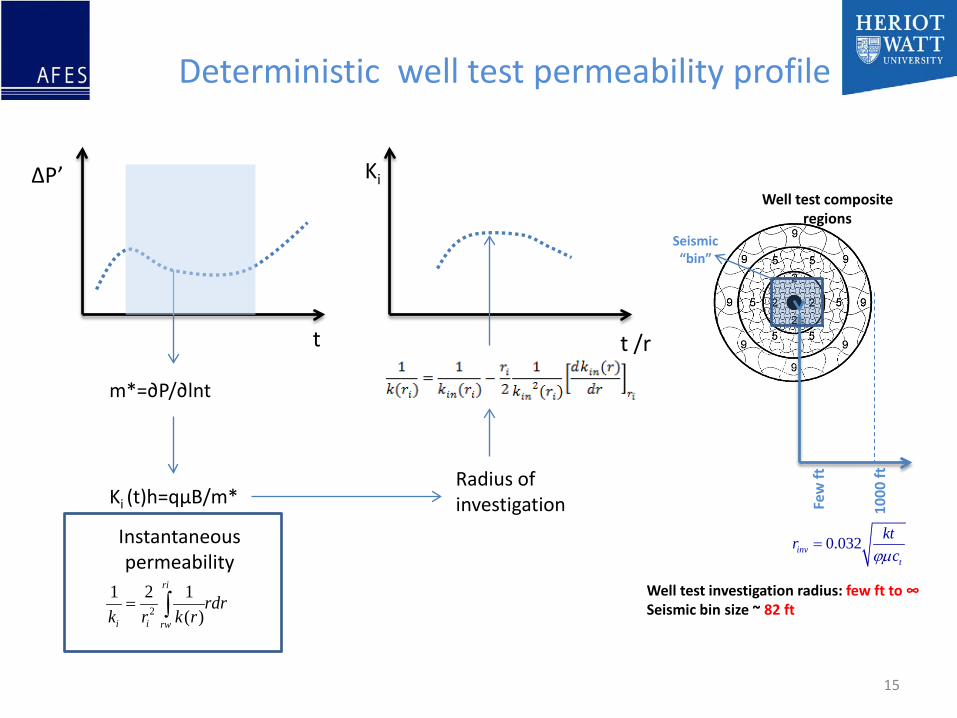
m*=∂P/∂lnt
Ki (t)h=qμB/m*Radius of investigation
2
1 2 1( )
ri
i i rw
rdrk r k r= ∫
∆P’
t t /r
Ki
Instantaneous permeability
Deterministic well test permeability profile
Few
ft
1000
ft
0.032invt
ktrcϕµ
=
Well test composite regions
Seismic “bin”
Well test investigation radius: few ft to ∞Seismic bin size ~ 82 ft
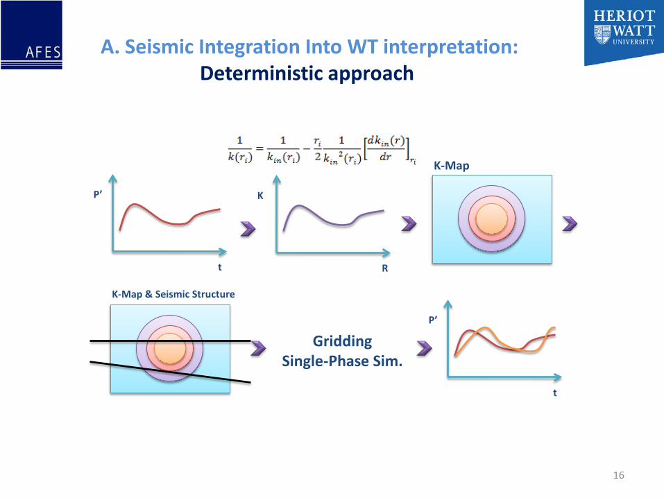
A. Seismic Integration Into WT interpretation:Deterministic approach
P’
t
K
R
K-Map
K-Map & Seismic Structure
P’
t
GriddingSingle-Phase Sim.
16
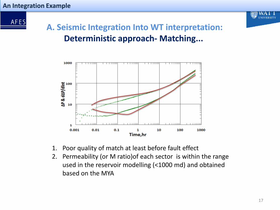
A. Seismic Integration Into WT interpretation:Deterministic approach- Matching...
1. Poor quality of match at least before fault effect2. Permeability (or M ratio)of each sector is within the range
used in the reservoir modelling (<1000 md) and obtained based on the MYA
17
An Integration Example
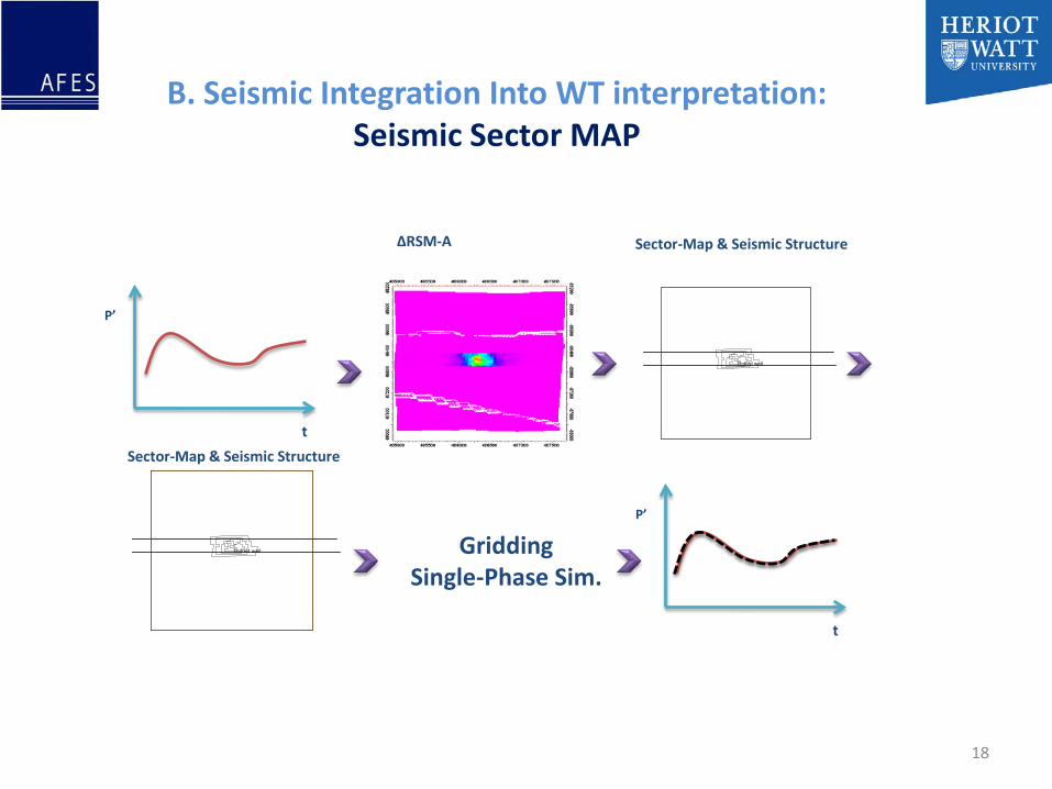
B. Seismic Integration Into WT interpretation:Seismic Sector MAP
P’
t
P’
t
Tested well
Tested well
Sector-Map & Seismic Structure∆RSM-A
Sector-Map & Seismic Structure
18
GriddingSingle-Phase Sim.
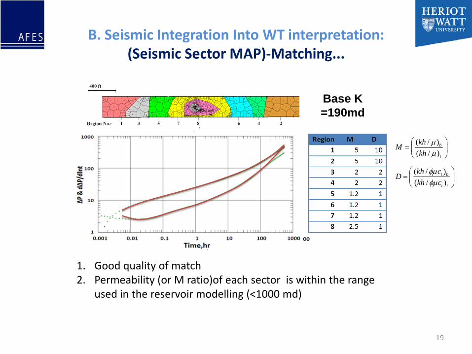
Base K =190md
1. Good quality of match2. Permeability (or M ratio)of each sector is within the range
used in the reservoir modelling (<1000 md)
B. Seismic Integration Into WT interpretation:(Seismic Sector MAP)-Matching...
19
( / )( / )
t b
t i
kh cDkh c
φµφµ
=
( / )( / )
b
i
khMkh
µµ
=
50 100 150 200 250
50
100
150
200
250
-0.15
-0.1
-0.05
0
0.05
0.1
0.15
0.2
50 100 150 200 250
50
100
150
200
250 -2
-1
0
1
2
3
4
5
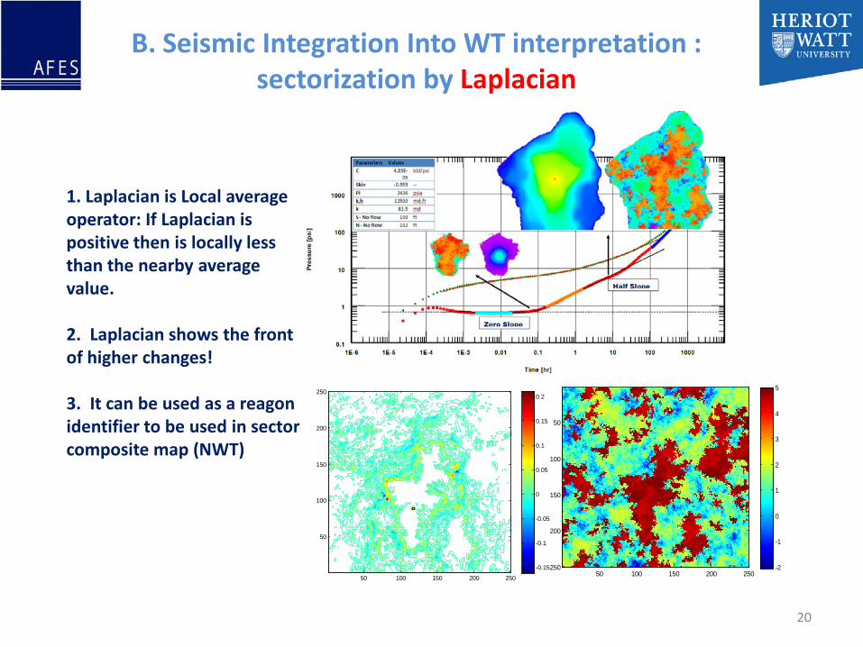
B. Seismic Integration Into WT interpretation : sectorization by Laplacian
1. Laplacian is Local average operator: If Laplacian is positive then is locally less than the nearby average value.
2. Laplacian shows the front of higher changes!
3. It can be used as a reagonidentifier to be used in sector composite map (NWT)
20
outline
• Overview of Well Testing– Information obtained from well test– Uncertainty in model recognition
• An Integration Example– Stratigraphic discontinuity detection (4D seismic)– Numerical well-test Interpretation
• Deterministic approach• Inverse Approach
• Conclusions
21
Conclusion
• Well test interpretation was constrained• Larger faults mapped out using 3D & 4D seismic • Permeability baffles were realized by 4D signal• Numerical well testing was performed using the information
from seismic data – reduce the uncertainty in model detection
• 4D& 3D seismic help sectorize the map used in numerical well testing software
• reasonable match obtained by integration of numerical well testing and seismic
22

Acknowledgements
• Schlumberger
• Weatherford
• Kappa
23
References
• Boutad de la Comb, J.L., Akinwunmi, O., 2005. Use of DST for effective dynamic appraisal: case studies from deep offshore west Africa and associated methodology, SPE 97113
• Gringarten, A., 2009. From straight lines to deconvolution - the evolution of the state-of-the-art in well test analysis, EAGE/SPE joint workshop of well testing and seismic, Berlin
• Feitosa,G.S., Lifu, C., Thompson, L.G. and Reynolds, A.C.,1994. Determination of permeability distribution from well-test pressure data, SPE 26047
• MacBeth, C., Floricich, M. and Soldo, J., 2005. Going quantitative with 4D seismic analysis, Geophysical Prospecting, 54, 303–317
• Sahni, A., Kelsch, K., Samorn, H., Boonmeelapprasert, C., 2007. Integrating pressure transient test data with seismic attribute analysis to characterize an offshore fluvial reservoir, SPE 110272
• Zheng, S.Y, Corbett, P.W.M. and Emery, A., 2003.Geological interpretation of well test analysis: case study from a fluvial reservoir in the gulf of Thailand, Journal of Petroleum Geology, Vol. 26(1)
• Zheng, S.Y, Legrand,V.M. and Corbett, P.W.M. ,2007. Geological model evaluation through well test simulation: a case study from the Wytch Farm oilfield, southern England, Journal of Petroleum Geology, Vol. 30(1), pp 41-58
24