AN EXAMINATION OF THE STATISTICAL DISCREPANCY · PDF fileAN EXAMINATION OF THE STATISTICAL...

27AN EXAMINATION OF THE STATISTICAL DISCREPANCY

Journal of Applied Economics, Vol. IV, No. 1 (May 2001), 27-61

AN EXAMINATION OF THE STATISTICALDISCREPANCY AND PRIVATE INVESTMENT

EXPENDITURE*

CHRISTOPHER BAJADA

School of Finance and EconomicsUniversity of Technology, Sydney Broadway

The statistical discrepancy is often used to gauge the reliability of national accounts data.Particularly since the mid-1980’s the statistical discrepancy in Australia has grownsignificantly in size and variance. In this paper we demonstrate that the overwhelmingcontribution to the size of the statistical discrepancy is mismeasurement of private investmentexpenditure. We demonstrate that this mismeasurement not only adds to the volatility ofinvestment but may have a significant impact on the volatility of the business cycle ingeneral.

JEL classification codes: E32, C82Key words: statistical discrepancy, national accounts, investment, businesscycles

I. Introduction

In the Australian National Accounts (ANA), the Australian Bureau ofStatistics (ABS) estimates the size of economic activity in Australia bycalculating Gross Domestic Product (GDP). There are three alternative

* I would like to thank Ross Milbourne, Graham Voss, Jorge Streb, Jayne Baker, and RossHarvey for their comments and information pertaining to the methods of data collection. Iwould also like to thank two anonymous referees for their helpful suggestions. Naturally,any errors and omissions are my own.

28 JOURNAL OF APPLIED ECONOMICS

measures by which the ABS calculates GDP1 : (1) the expenditure approach;(2) the income approach; and (3) the production approach. In principle thesethree methods should yield the same results but in practice they do not. TheABS statistician is required to introduce a "Statistical Discrepancy" item inthe ANA in order to reconcile the income side with the expenditure side.

The statistical discrepancy in the national accounts has in recent yearsincreased significantly both in mean and variance. Since 1970 the discrepancyhas averaged 2% of GDP and in more than 36% of quarters, the growth in thestatistical discrepancy was greater than or equal to the growth in GDP. Unlikemost of the OECD countries, Australia’s statistical discrepancy is quite largeand it has been so particularly since the mid-1970’s. In recent years, particularlysince the mid-1980’s, the statistical discrepancy has been predominantlypositive and growing. Evidently the implication of this are that one or moreof the major expenditure components in the ANA, such as investment andconsumption, are under-reported. Clearly there is an issue regarding accuracyand reliability.

The question of how accurate and reliable are the national accounts isimportant for many reasons. It is of considerable policy interest to haveaccurately measured economic data because these are intended to providenot only a comprehensive and systematic summary of economic activity, butalso a resource from which to gauge economic policies. Secondly, the existenceof a non-negligible and volatile statistical discrepancy has implications notonly for investigating economic theories but implications also for the business

1 Recently the ABS implemented the System of National Accounts (SNA93) into the ANA.While significantly contributing to an improvement in the measurement of national output,the changes have only had a small impact on the movement of GDP (ABS, 1998). Thethree alternative measures of calculating GDP are no longer explicitly published, replacednow by a single measure. To ensure that the components do balance, the statisticaldiscrepancy is now allocated to each of the components based on information from input-output tables. Although the statistical discrepancy is no longer explicitly reported, an estimateof its size is nevertheless possible to construct.


cycle in general. Consequently it is important to know something about thestatistical properties of the discrepancy.

Weale (1992) proposed a maximum likelihood procedure to identifywhether income or expenditure measures of GDP contribute most to the sizeof the statistical discrepancy. The aim of this paper is twofold. First, togeneralise the procedure in order to determine which component(s) of thenational accounts have contributed most to the statistical discrepancy. Second,to investigate the implication that such mismeasurement may have on thebusiness cycle.

The remainder of this paper is organised as follows. Section II addressesthe statistical properties of the discrepancy. In Section III we extend on Weale's(1992) methodology. Our findings suggest that private investment has beensubject to the most measurement error and consequently if measured correctlyprivate investment is more volatile than existing measures suggest. Thiscoincides with previous results which suggest that actual investment data isnot as volatile as theory might suggest (Guest and McDonald, 1995). Theseresults are summarised in Section IV. In Section V we demonstrate that ifmeasured correctly, investment may have a significant impact on the natureof the business cycle. Section VI presents our major conclusions.

II. Analysing the Statistical Discrepancy

In recent years there has been a growing concern about the accuracy andreliability of the national accounts (see McDonald, 1973,1975; Johnson, 1982;Matthews, 1984; Lim, 1985; Young, 1987). Claims suggesting the quality ofthe national accounts have been significantly undermined in recent years aregenerally supported by the large and volatile statistical discrepancy. Perhapsthe volatility of the statistical discrepancy should be a major concern to thosewho use and interpret the national accounts. It is clear though, that the largerthe swings in the statistical discrepancy, the larger are the inconsistencies orquarter-to-quarter growth rates of income and expenditure estimates of GDP


over time. The grounds for such concern are primarily two fold; (1) the datasource and procedures used to construct missing observations are unavailableto the statistician from existing data sources (De Leeuw, 1990), and (2) thetiming of the recording of transactions (McDonald and Monk, 1975).

A. Data Sources and Procedures

It is generally costly to collect information frequently, so naturally theABS makes use of interpolations and extrapolations in order to construct, forexample, quarterly observations if it only has annual data.2 Sometimes theABS is dependent on alternative data sources in the construction of particularvariables which often come from surveys of businesses and households, theAustralian Taxation Office and government data. At other times it is necessaryto transform the data into an appropriate national accounting basis andmeasurement errors are likely to arise particularly if the available data sourcesdo not conform with the definitions implied in the national accounts.Furthermore, these approximations may become more unreliable in a rapidlychanging environment. However not all components of the national accountsare equally susceptible to these sort of measurement problems. In fact,components of the national accounts which measure government consumptionand investment expenditure are likely to be measured more accurately thanprivate consumption and investment expenditure as the latter are based onsurveys which at times are incomplete, while the former are usually extractedfrom government source data which contain the actual expenditures.

To highlight the sources of potential measurement problems in the

2 The use of interpolation techniques are not without their problems. It has been shownby Milbourne and Bewley (1992) that a quarterly time series constructed using linearinterpolation of annual data will, in a dynamic framework, appear to be Granger caused bythe statistical discrepancy. This is because when quarterly data are interpolated from annualdata, the quarterly estimates are in fact functions of the annual benchmarks from whichthey were constructed. Trying to establish causal relationships then is clearly not appropriate.


compilation of the national accounts data, it is necessary to have a brief lookat the measurement of each of the major components. At the outset it is possibleto give a preliminary ordering of the components on the basis of reliability. InSection IV we implement a maximum likelihood procedure to construct astatistical ordering to either confirm or reject the conclusions drawn in thissection. In Table 1 we outline the data sources for each of the majorcomponents in the national accounts and the deficiencies which may arisefrom their measurement. These are briefly discussed below.

Table 1. Data Sources and Reliability

Variable Data Sources (a) Problems

HouseholdConsumptionExpenditure

Household ExpenditureSurvey; Retail Census(every 4 years); ServiceIndustry Surveys; Surveyof Retail Trade;Hospitality IndustrySurvey; Census ofPopulation and Housing;Building Activity Survey;Survey of Motor Vehicleuse; Transport IndustrySurvey.

Collection of data is takeninfrequently andextrapolations, particularlyfrom censuses, have to bemade using less completedata. Independent datasources may not alwaysconform with the definitionsof expenditure required bythe national accountant butare not as frequent as in thecase of private investmentexpenditure.

GovernmentConsumptionExpenditure

Public Accounts Ledgers;Budget papers; AuditorGeneral's report;

Most data is sourced directlyfrom government records andas a result the quality of the


CommonwealthDepartment of Financeand Administration;Commonwealth GrantsCommission; StateGovernment monthly andquarterly statements.

Table 1. (Continue) Data Sources and Reliability


data is much better than forprivate consumption.However a number of surveysare used for local government(as there are many of these)data which unfortunately isnot as reliable as data comingfrom State andCommonwealth governmentdepartments.

PrivateInvestmentExpenditure

Annual and PeriodicSurveys of Industries;Sub-annual surveys ofbusinesses acrossindustries; AustralianTaxation Office data; ABSgovernment finance data;Building Activity Survey;Household ExpenditureSurvey; Survey of NewCapital Expenditure;Engineering ConstructionSurvey; Survey ofInformation Technology.

There is a significant use ofinterpolations andextrapolations in thecollection of privateinvestment expenditure.Many independent surveysdot no usually conform withthe definitions used in thenational accounts nor do theycover the range ofinvestments that are stated asmeasured in the accounts.Extrapolation of data fromparts of one industry aremade into another for whichdata is not available.


Table 1. (Continue) Data Sources and Reliability


GovernmentInvestmentExpenditure

Annual Report ofPublic non-financialCorporations; Auditor'sGeneral Reports; JointABS / CommonwealthGrants Commission;Commonwealth and StateBudget papers; Survey ofExpenditure on FixedAssets; CommonwealthDepartment of Financeand Administration.

As with governmentconsumption, the data sourcesare directly taken fromgovernment records.However, for localgovernment there is a moreextensive use of surveyswhich undoubtedlyintroduces the possibility ofmeasurement errors. As withgovernment consumption, theextent of these errors are notsignificant.

Imports andExports

ABS International TradeStatistics; ABS QuarterlySurvey of PrincipalTransport Enterprises;ABS Quarterly Survey ofInternational Trade inservices; Department ofDefence documents;Survey of ReturnedAustralian travellers andInternational VisitorSurvey.

Mainly sourced from ABSInternational Trade Statistics,this data source covers mostflows of imports and exports.Supplementary surveys arealso used to measure, forexample, goods procured inforeign ports. As thesesupplementary surveys aresmall in number, the extent oflikely measurement errors areexpected to be small.

Notes: (a) Identifies the major data sources for each variable. The ABS does use other, lessexhaustive surveys which are not mentioned here.


Consumption

Much of the data for private consumption expenditure is benchmarkedperiodically from Retail Censuses which are often adjusted for sales whichare out of the scope of the census. The last census was conducted in 1991-92and this benchmark is moved forward using data from a number of sourcesnamely, the Monthly Surveys of Retail Trade, Service Industry Surveys,Household Expenditure Surveys (HES) and Public Finance Statistics. Howevernot all these data sources are collected frequently and in some yearsextrapolations have to be made using less complete data. For example, theexpenditure on new motor vehicles is estimated using information in Glass'sGuide for Passenger Vehicles and automotive magazines and extrapolatedusing information collected for the CPI. By multiplying the estimated numberof sales by the estimated average price, the national accountant obtains anestimate of expenditure on new motor vehicles.

Government final consumption expenditure covers net outlays by generalgovernment on goods and services such as defence, public order and education.Since on most occasions these are provided free of charge or at a small markup on costs, the output has no directly observable market value and so it isvalued in the national accounts at its cost of production. Commonwealth andState government expenditure are sourced directly from public account ledgers,budget papers, Auditor's General Reports and supplementary departmentaldocuments. For local government, data is collected from either theCommonwealth Grants Commission, the Department of Local Government,or from ABS surveys of local government activities. Since governmentconsumption is predominantly measured directly from expenditure records,it implies that this variable is more reliably measured than is privateconsumption expenditure, which relies more heavily on surveys. For this reasongovernment consumption expenditure is likely to contribute less to the sizeof the statistical discrepancy than is private consumption expenditure.


Investment

Many data sources are used in the construction of investment expenditurenamely annual and periodic surveys of industries, sub-annual surveys ofbusinesses across industries, Australian Tax Office data and ABS governmentfinance data. However in many cases these collections are taken infrequentlyand extrapolations of the data are necessary. In other circumstances the nationalaccountant makes extensive use of benchmarks from which other indicatordata is extrapolated. For example, the value of alterations and additions tobuildings are estimated using data from regular surveys of building activityand from the periodic HES. However a significant part of alterations andadditions are not covered in the Building Activity Survey. Nevertheless thisdata is used as an indicator to move forward benchmark estimates ofexpenditure obtained from the HES. Similar problems are true for expendituremeasures of machinery and equipment. Quarterly estimates are interpolatedbetween and extrapolated from taxation data using the Quarterly Survey ofNew Capital Expenditure. For example, annual estimates of expenditures onfarm machine and equipment are based on data from the Tractor MachineAssociation, which unfortunately does not collect data from all industries.Expenditure in industries which do not fall in the scope of this survey areestimated by applying the average movements from industries which arecovered by the survey to those that are not. Clearly these approximationsappear to be more ad hoc for the measurement of private investmentexpenditure than they are for private consumption expenditure.

For Commonwealth and State government investment expenditure, datais collected from administrative by-product sources such as financialstatements prepared by the Minister of Finance, Commonwealth and Statebudget papers, Auditors'- General Reports, Commonwealth Department ofFinance and Administration ledgers, supplementary departmental documents,and by direct collection from general government units. Since governmentfinal investment expenditure is predominantly sourced directly from


government expenditure records it implies that this is more reliably measuredthan is private investment expenditure.

Exports and Imports

The main source of data for imports and exports are from the ABSInternational Trade Statistics (ITS) compilation, which are derived frominformation provided by the importers or exporters, or their agents, to theAustralian Custom Services. Although such data covers predominantly mostof import and export flows, there are however some flows which theinternational trade statistics do not capture such as goods procured in foreignports. Therefore a number of other data sources are used to supplement theInternational Trade Statistics. These include the ABS's quarterly Survey ofPrincipal Transport Enterprises, the ABS's quarterly Survey of InternationalTrade in Services, quarterly data from the Department of Defence on exportsand imports of defence equipment and monthly and quarterly advice from theReserve Bank of Australia.3 Although there are some issues regarding thereliability of these supplementary surveys, the data collected for imports andexports are reasonably well measured since most of the data is sourced fromITS.

It appears from this discussion that the various aggregates in the nationalaccounts are susceptible to various reliability concerns. In particular privateconsumption and investment expenditure are likely to be most unreliablyestimated, with investment expenditure contributing more to the size of thestatistical discrepancy than would consumption. Less likely to be susceptibleto measurement error are government expenditure components, imports andexports for reasons already discussed. In order to test this claim, in the

3 The survey of Principal Transport Enterprises provides information on offshore installationsof ships, aircraft and satellites operating in Australian and international waters; and theReserve Bank of Australia provides information on gold sales and purchases by non-residents.


following section we implement a statistical procedure which will help orderthe components of the national accounts likely to be contributing most to thesize of the statistical discrepancy in Australia.

B. Timing Issues

The second area of concern relating to the accuracy and reliability of thenational accounts are the timing of recording of transactions. Directobservations of the early revisions in the statistical discrepancy highlights theexistence of timing problems. When the recording of transactions are madewith some delay, the effects show up in the statistical discrepancy ascombinations of volatility and seasonality. The sensitivity of the timing problemmay be illustrated by the following example. Suppose that in June 1999 therecording of a particular transaction ($100m) had been delayed by one quarter.This would affect three quarterly growth rates centred on the quarter at whichthe delayed transaction is recorded. The measured effects on the growth rateswould be – 0.09%, 0.19% and – 0.1% respectively. The effects on individualcomponents in the national accounts would be much larger (Johnson, 1982).

However this is predominantly a problem in the early stages of revisionsof the national accounts. After the release of preliminary figures, nationaleconomic data are subject to a further eight revisions as more accurate andtimely information becomes available. Although timely data is not a perplexingissue after two years, the statistical discrepancy does exhibits additionalvolatility and seasonality within this two year period, in fact more so fromsome variables than others. For example, income taxation is a source ofstatistical information which is used in the national accounts but is availablewith a lag. This lag is approximately two years for companies and about oneyear for individuals, sole traders, partnerships and trusts. Prior to 1978-79this latter group was also subject to a 2 year lag.

Much of the volatility of the statistical discrepancy after timely correctionshave been made are predominantly measurement errors arising from inadequate


surveys and samples. In fact, since the mid-1970’s the statistical discrepancyhas increased significantly in size and volatility suggesting a growth in thesemeasurement errors. Figure 1 plots the real quarterly statistical discrepancysince September 1959.

-4000.00

-3000.00

-2000.00

-1000.00

0.00

1000.00

2000.00

3000.00

4000.00

Sep-59

Jun-62

Mar-65

Dec-67

Sep-70

Jun-73

Mar-76

Dec-78

Sep-81

Jun-84

Mar-87

Dec-89

Sep-92

Jun-95

$m

Figure 1. Real (at 1989/90 prices) Statistical Discrepancy

III. Statistical Model

Since by definition, GDP is the market value of goods and servicesproduced in any economy over a period of time, we can define aggregateexpenditure as the sum of the smaller expenditure components. Since in theabsence of measurement error, GDP(E) = GDP(I), it must be true that thesum of the smaller income components equal the sum of all the expenditurecomponents. The asterisks defines the true value of the aggregates.


**OS* TSGW ++≡

*)I(GDP≡

where*)E(GDP = the expenditure measure of GDP

*)I(GDP = the income measure of GDP

*pC = Private final consumption expenditure

*gC = Public final consumption expenditure

*pI = Investment (private gross fixed capital expenditure +

+ increases in stocks)*gI = Public gross fixed capital expenditure

*X = Exports of goods and services*M = Imports of goods and services*W = Wages, salaries and supplements

*OSG = Gross Operating Surplus

*TS = Indirect taxes less subsidies

(1)

Each component in (1) is subject to measurement error for reasonsdiscussed in Section II. In the national accounts the following expression holds

XIICCTSG gpgpOS ++++=++

)E(GDP GDP(I) = + SD (2)

***g

*p

*g

*p

* MXIICC)E(GDP −++++≡

W − M + SD


where SD denotes the statistical discrepancy.Since the statistical discrepancy is defined as the sum of the measurement

error of each component of aggregate demand, we can write (2) as

*)I(GDP=

(3)

TSGwmxIgIpcgcp OSSD ε+ε+ε+ε+ε−ε−ε−ε−ε−=

cpp*p CC ε−= ;

cgg*g CC ε−= ;

Ip*p II ε−= p

; Kgg

*g II ε−= ;

x* XX ε−= ;

where

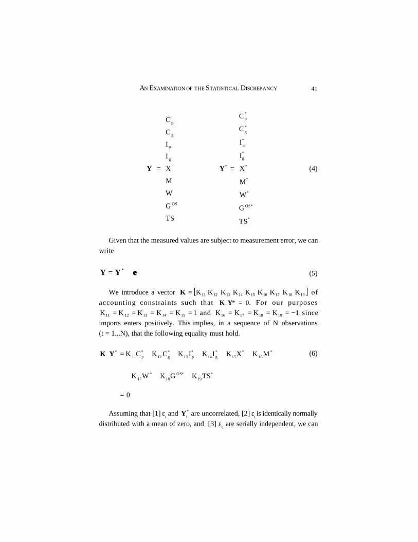
We apportion SD betweenusing a generalisation of Weale (1992).4 We begin with a (9×1) vector ofaccounting aggregates Y as measured by the national accounts and anothervector , unobservable but true measures of the same aggregates.

T SGwmxIgIpcgcp and , , , , , , , OS εεεεεεεεε

4 Since the statistical discrepancy is a measure of ‘net’ error this apportionment is at bestan approximation of the truth. It will however give a more accurate relative contribution ofeach component of aggregate demand on the size of the statistical discrepancy.

*Y

+ (X − εx) − (M − εm)

= (W − εw) + (Gos − εGos) + (TS − εTS)

εIg; X* = X − εx;

M* = M − εm; W* = W − εw; GOS* = GOS − εGos; TS* = TS − εTS

GDP(E)* = (Cp − εcp) + (Cg − εcg) + (Ip − εI) + (Ig − εKg) +

p;


=

=

*

*OS

*

*

*

*g

*p

*g

*p

*

OS

g

p

g

p

TS

G

W

M

X

I

I

C

C

TS

G

W

M

X

I

I

C

C

YY (4)

Given that the measured values are subject to measurement error, we canwrite

εε+= *YY (5)

We introduce a vector [ ]191817161514131211 K K K K K K K K K=K ofaccounting constraints such that K Y* = 0. For our purposes

1KKKKK 1514131211 ===== and 1KKKK 19181716 −==== sinceimports enters positively. This implies, in a sequence of N observations(t = 1...N), that the following equality must hold.

*16

*15

*g14

*p13

*g12

*p11

* MKXKIKIKCKCK ++++++=YK

*19

*OS18

*17 TSKGKWK +++

(6)

= 0

Assuming that [1] εt and *tY are uncorrelated, [2] εt is identically normally

distributed with a mean of zero, and [3] εt are serially independent, we can


estimate the true unobserved values of each of the aggregates in (4) by

maximising the following log-likelihood function:5

subject to the constraint (6).The constrained quadratic loss function may be written as

where Z = Y - Y* and V is a (9 x 9) unknown variance covariance matrix.The accounting constraint (6) may alternatively be written as KZ - KY = 0

since KY* = 0. Therefore

Differentiating and solving with respect to Z gives

Pre-multiplying by K, substituting KY for KZ and solving for λ gives:

5 We assume serial independence because the data set used does not contain any observationswhich are under revision. For this reason the timing concerns on Section II.B does notpose a problem in our estimation.

( * ,L YVY (7)

*1T

21

KYZVZ λ−= −L (8)

( )KYKZZVZ −λ−= −1T

21L (9)

λ= TVKZ (10)

( ) KYKVK1T −

=λ (11)

) ( ) (−π−= ln2N

2ln2N

V ) ( ) ( −− −1T*

21

YVYY )− *Y


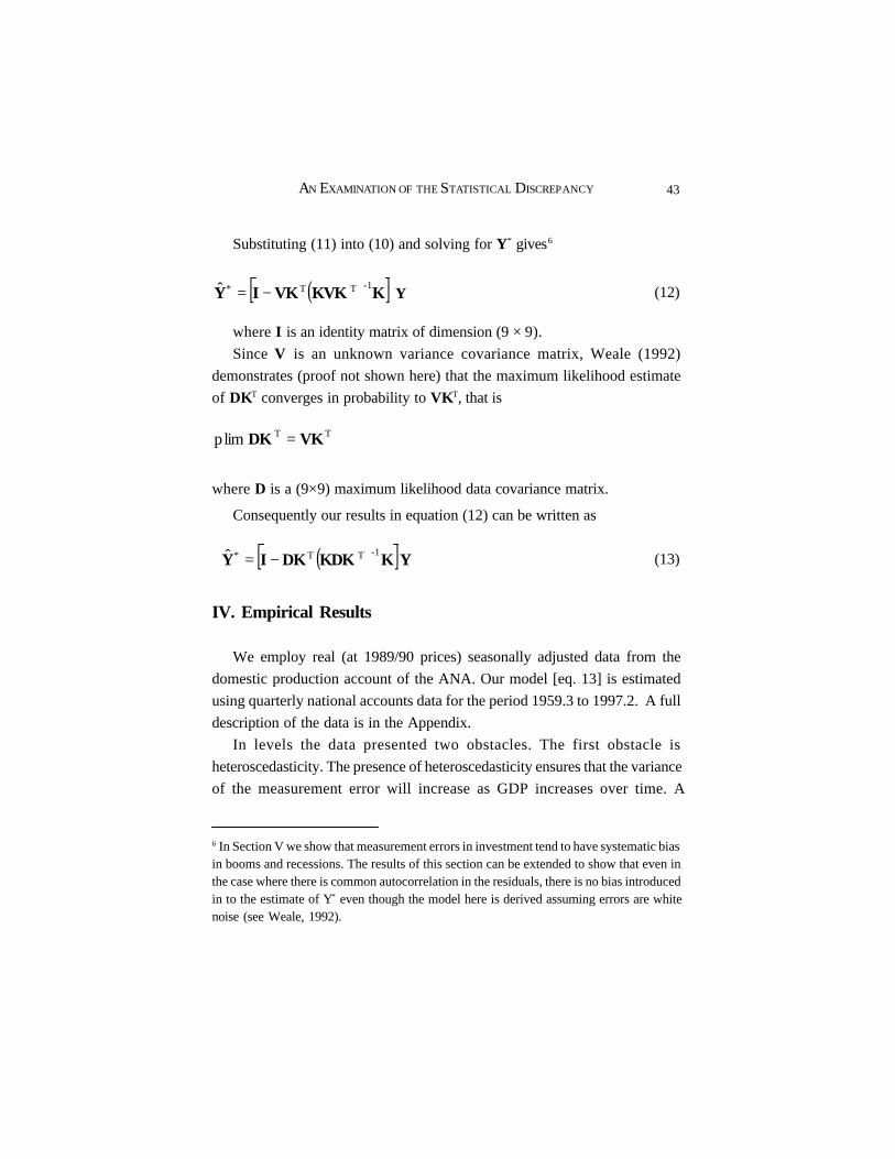
Substituting (11) into (10) and solving for Y* gives6

where I is an identity matrix of dimension (9 × 9).Since V is an unknown variance covariance matrix, Weale (1992)

demonstrates (proof not shown here) that the maximum likelihood estimateof DKT converges in probability to VKT, that is

where D is a (9×9) maximum likelihood data covariance matrix.

Consequently our results in equation (12) can be written as

IV. Empirical Results

We employ real (at 1989/90 prices) seasonally adjusted data from thedomestic production account of the ANA. Our model [eq. 13] is estimatedusing quarterly national accounts data for the period 1959.3 to 1997.2. A fulldescription of the data is in the Appendix.

In levels the data presented two obstacles. The first obstacle isheteroscedasticity. The presence of heteroscedasticity ensures that the varianceof the measurement error will increase as GDP increases over time. A

6 In Section V we show that measurement errors in investment tend to have systematic biasin booms and recessions. The results of this section can be extended to show that even inthe case where there is common autocorrelation in the residuals, there is no bias introducedin to the estimate of Y* even though the model here is derived assuming errors are whitenoise (see Weale, 1992).

( )[ ]YKKVKVKIY-1TT*ˆ −= (12)

TT limp VKDK =

(13)( )[ ]YKKDKDKIY ˆ -1TT* −=

Y


logarithmic transformation of the data has the advantage of reducing thepresence of heteroscedasticity by compressing the scale in which the variablesare measured. However using a logarithmic transformation of the data disturbsthe accounting constraint given by (6). The second obstacle is non-stationarity.This is generally overcome by first differencing the data.

To ensure that our model produces consistent results with Weale’ssimplified model, we require an alternative data transformation.7 For thesmaller expenditure aggregates, namely Cp, Cg, Ip, Ig, X and M, we take firstdifferences as a proportion of GDP(E). For the smaller income aggregates,namely W, Gos and TS, we take first differences as a proportion of GDP(I).These transformations ensure that [1] the accounting constraint (6) is notdisturbed, [2] the data is stationary.8 Testing for the presence of non-stationaritywe find that in levels all the variables exhibit evidence of a unit root but arestationary under the new transformation. These results are reported in Table2; and [3] the sum of the proportion, δ, of the statistical discrepancy contributedby each of the smaller national accounting aggregates sum to the proportionscontributed by the larger aggregates, namely GPD(I) and GDP(E), that is,

7 Weale (1992) used logarithmic first differenced data since the methodology is unaffectedusing this particular data transformation in a two variable case.

8 The model may alternatively have been estimated using a recursive process where theestimates of GDP(I*) = GDP(E*) from the first round could have been used to divide all thecomponents in the second round by a single number. The estimates are unaffected eitherway.

)E(YNXGIC δ=δ+δ+δ+δ and

where C = Cp; I = Ip; G = Cg + Ig and NX = X - M

We are now in a position to construct maximum likelihood estimates for thetrue but unobservable values of national output. We do so by estimating

)I(YTSGW OS δ=δ+δ+δ


Table 2. Dickey-Fuller Unit Root Tests

Levels First Difference

Variable

Yt

q

Constant

No Trend

α(1) = 0

τ

Constant

Trend

α(1) = α(2) = 0

F-test Φ3 d

Constant

No Trend

α(1) = 0

τ

Constant

Trend

α(1) = α(2) = 0

F-test Φ3

Cp 6 3.26 5.30 5 -4.01 11.64Cg 3 -0.05 3.35 5 -3.81 09.58Ip 10 -0.80 8.00 11 -4.49 10.70Ig 1 -2.22 2.59 8 -4.42 15.47X 9 2.99 4.58 8 -4.70 11.52M 12 2.15 2.83 12 -4.43 09.83W 0 0.44 2.34 11 -2.95 07.08Gos 0 0.42 3.15 7 -4.70 11.75T S 11 1.52 2.85 9 -4.17 8.65

GDP(I) 4 1.39 3.31 12 -2.95 6.87GDP(E) 2 1.48 2.64 12 -2.95 7.77

Notes: a) Columns 3 and 4 have the following Dickey-Fuller specifications:

and Columns 6 and 7 have the following specifications (where t = time trend)

b) Null hypotheses are found at the head of each column. α(1) = 0 in columns 3 and 6 areτ-tests and in columns 4 and 7, α(1) = α(2) = 0 are unit root tests with non-zero drift(F-test Φ 3). The critical τ-statistic for columns 3 and 6 is -2.57, and the critical F-test Φ 3 forcolumns 4 and 7 is 5.34.

c) d and q were chosen as the highest lag from the autocorrelation function of the firstdifferenced series at the 95% confidence interval.

∑=

ε+−+α+−α+α=q

1i titYib1tY10tY 2 t

∑=

ε+−∆+α+−α+α=∆d

1i titYibt21tY10tY

t


equation (13) using the newly transformed data, and calculating the contributionto the total statistical discrepancy from the measurement errors in GDP(E) andGDP(I) by − Y.9 The proportion of the statistical discrepancy attributed toeach of these two inconsistent measures of national output are given in Table3. Also in Table 3 is a measure of how sensitive changes in sample size are onthe measurement of these proportions.

Y *ˆ

9 To ensure that both our model and Weale’s model produce consistent results, GDP(I) andGDP(E) are measured in quarterly growth rates. This is consistent with Weale’s logarithmicfirst differencing of the data.

10 Weale (1992) also finds the expenditure measure contributes most to the size of thestatistical discrepancy in the United States.

Table 3. Proportion of the Statistical Discrepancy Contributed by GDP(I)and GDP(E)

No. of end-point observations removed from data set

Variable δ 5 10 15 20 25 30 35

GDP(E) 0.90 0.91 0.91 0.90 0.91 0.92 0.92 0.93

GDP(I) 0.10 0.09 0.09 0.10 0.09 0.08 0.08 0.07

Notes: δ denotes the proportion of the total measurement error attributed to either GDP(E)or GDP(I). Columns 3 to 9 represent the same proportion except the number of end-pointobservations dropped from the data set is denoted at the head of each column.

Table 3 suggests that the statistical discrepancy is predominantlyunmeasured aggregate expenditure. Approximately 90% of the statisticaldiscrepancy is the result of measurement error in GDP(E) with 10% accountedfor by mis-measurement in aggregate income.10 These results appear relatively


robust to changes in sample size as shown in columns 3-9 in Table 3. Varyingthe sample size has no significant effect on these results.

In Table 4 we present results for the generalised model. The proportion ofthe statistical discrepancy contributed by each of the smaller nationalaccounting aggregates are presented in column 1 of Table 4. As expected thesum of the contributions from Cp, Cg, Ip, Ig, X and M sum in absolute value tothe contributions for GDP(E). Similarly the contributions from W, Gos andTS sum in absolute value to the contribution for GDP(I). The proportion ofthe statistical discrepancy contributed by GDP(E) and GDP(I) are thosereported in Table 3.

Table 4. Proportion of the Statistical Discrepancy Contributed by theComponents of Aggregate Demand

Variable δ Variable δ Variable δ Variable δ

Cp 0.06 Cp 0.06 Cp 0.06 Cp 0.06Cg 0.04 Ip 0.69 Ip 0.69 Ip 0.69Ip 0.69 Cg + Ig 0.09 Cg + Ig 0.09 Cg + Ig 0.09Ig 0.05 X 0.04 X – M 0.06 X – M 0.06X 0.04 M 0.02 W 0.03 GDP(I) 0.10M 0.02 W 0.03 Gos 0.06W 0.03 Gos 0.06 T S 0.01Gos 0.06 T S 0.01T S 0.01

These results demonstrate, as was suggested in Section II, that governmentdata is less likely to be influenced by measurement error than is non-government data as sources for government data are much more reliable.Public consumption expenditure was found to contribute approximately 4%of total measurement error in the national accounts. Trade data appears to do

(1) (2) (3) (4)


relatively well, as was also expected from Section II, with imports contributingthe least to the measurement error (2%) and exports contributing 4% of totalmeasurement error.

Private final consumption and private investment expenditure do notperform so well. Private consumption expenditure contributed 6% to the totalmeasurement error while private investment expenditure contributed astaggering 69% of total measurement error.11 This is easily reflected in thequality of the surveys and samples used to compile private investment andconsumption expenditure. The greater use of interpolations and extrapolationsin the construction of investment in association with a large number ofinadequate data sources is reflected in this result. Private investment is by farthe most incorrectly measured series in the ANA. The extent of themeasurement error in investment (74%) may have significant impact of thevolatility of the business cycle (to be discussed below) particularly if thevolatility of correctly measured private investment is greater than the volatilityof existing measures.12

In columns 2 and 3 of Table 4 an exercise is undertaken to reinforce therobustness of these results. In column 2 the sum of Cp, I p, G (= Cg + Ig), X andM in absolute value sum to GDP(E) as does the sum of Cp, I, G and NX(= X – M) [column 3]. From either disaggregation [columns 1, 2 or 3] privateinvestment expenditure contributes to approximately 74% of the size andvariation of the statistical discrepancy. It is to the implications of such mis-

11 The model produces consistent and robust results using time series variance because theaccounting constraint can be used in the model to purge the genuine volatility, leaving onlythe noise. This implies that although investment is a highly volatile series, the results of themodel do not depend on the volatility of the variables in the model. In fact there are greatervolatility in external flows of goods and services than there are for consumption expenditure,yet consumption expenditure contributes more to the size of the statistical discrepancythan do imports and exports.

12 Investment referred to here is the sum of private and public gross fixed capital expenditureand increases in stocks.


measurement, particularly private investment expenditure, that we now turn.

V. Mismeasurement of Investment

There have been a number of attempts (see Milbourne and Bewley, 1992;McKibbin and Morling, 1989; and Gregory, 1989) to determine whichaggregates in the national accounts have contributed most to the size andvariability of the statistical discrepancy. Gregory (1989) takes the view thatprivate sector saving-investment imbalances may explain most of themeasurement error in the national accounts. The premise is based on the viewthat public and external flows of goods and services are more likely to beaccurately measured than are private flows because good records of the dataexist.

McKibbin and Morling (1989) argue that the statistical discrepancy isunmeasured consumption expenditure. This argument is mistakenly premisedon a negative correlation found to exist between the statistical discrepancyand consumption. It is possible to demonstrate that such a correlation naturallyexists. Assuming the measurement error in consumption, εc (= εp + εg) iswhite noise, the covariance with the statistical discrepancy (SD), may bewritten as follows:

since E[SD] = 0, εc is white noise and SD = -εc - εI - εG - εX + εM

Similarly, it is possible to show that the covariance between the remainingexpenditure components and the statistical discrepancy are:

] ]C[EC [ ] ]SD[ESD [Ec,sd −−=σ

] ]C[EC(SD [E c* −ε+×=

c

2εσ−=

(14)

I

2I,sd εσ−=σ G

2G,sd εσ−=σ; ; X

2X,sd εσ−=σ ;

M

2M,sd εσ=σ

)]


Therefore, as long as ε is white noise the covariance of the statisticaldiscrepancy with private and public consumption and investment expenditureand exports should be negative. The covariance of the statistical discrepancywith imports should be positive. Table 5 presents the covariances betweeneach of the aggregates in the ANA and the statistical discrepancy. As expectedthe covariances have the right sign.

Table 5. Covariance of the Statistical Discrepancy with the ExpenditureComponents of the National Accounts

Covariance

Cp Cg Ip Ig X M

SD -0.47E-04 -0.35E-04 -0.38E-04 -0.20E-04 -0.65E-05 0.17E-05

Notes: The covariances are measured between each of the aggregate demand componentsas a proportion of GDP and the statistical discrepancy as a proportion of GDP.

Milbourne and Bewley (1992), using innovation analysis and variancedecomposition methods, find that a significant proportion of measurementerror in the national accounts arises from private sector investment expenditure.This appears to conform with our results that private investment expenditureis significantly mis-measured. What Milbourne and Bewley (1992) findsurprising in their results is that imports is the next most likely factorcontributing to the size of the statistical discrepancy. They expected, contraryto their findings, that imports (and exports) would be well measured for reasonsdiscussed in Section II.13 Our results support their expectation that importsand exports are well measured variables in the national accounts.

13 However their results are a function of the causal ordering of the variables used in theinnovation analysis. Although the results may change with different ordering, privateinvestment expenditure is by far the biggest contributing factor to the size of the statisticaldiscrepancy. However their methodology cannot attribute a specific quantity of the statisticaldiscrepancy to the components of the ANA.


There are several implications of these results particularly for investment.First, changes in investment usually conveys valuable information about thefuture movements in the economy and measurement error is only likely tobias such information. Second, changes in investment have a significant impacton the movements in national output and hence may suggest that the businesscycle is more volatile than is actually reported.

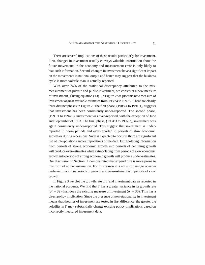
With over 74% of the statistical discrepancy attributed to the mis-measurement of private and public investment, we construct a new measureof investment, I* using equation (13). In Figure 2 we plot this new measure ofinvestment against available estimates from 1988:4 to 1997:2. There are clearlythree distinct phases in Figure 2. The first phase, (1988:4 to 1991:1), suggeststhat investment has been consistently under-reported. The second phase,(1991:1 to 1994:3), investment was over-reported, with the exception of Juneand September of 1993. The final phase, (1994:3 to 1997:2), investment wasagain consistently under-reported. This suggest that investment is under-reported in boom periods and over-reported in periods of slow economicgrowth or during recessions. Such is expected to occur if there are significantuse of interpolations and extrapolations of the data. Extrapolating informationfrom periods of strong economic growth into periods of declining growthwill produce over-estimates while extrapolating from periods of slow economicgrowth into periods of strong economic growth will produce under-estimates.Our discussion in Section II demonstrated that expenditure is more prone tothis form of ad hoc estimation. For this reason it is not surprising to observeunder-estimation in periods of growth and over-estimation in periods of slowgrowth.

In Figure 3 we plot the growth rate of I* and investment data as reported inthe national accounts. We find that I* has a greater variance in its growth rate(σ2 = 39) than does the existing measure of investment (σ2 = 30). This has adirect policy implication. Since the presence of non-stationarity in investmentmeans that theories of investment are tested in first difference, the greater thevolatility in I* may substantially change existing policy implications based onincorrectly measured investment data.


10000.00

12000.00

14000.00

16000.00

18000.00

20000.00

22000.00D

ec-8

8

Sep-

89

Jun-

90

Mar

-91

Dec

-91

Sep-

92

Jun-

93

Mar

-94

Dec

-94

Sep-

95

Jun-

96

Mar

-97

$m

Old Invest

New Invest

Figure 2. Measures of Investment: New (I*) and Existing

-20

-15

-10

-5

0

5

10

15

20

Dec

-88

Sep-

89

Jun-

90

Mar

-91

Dec

-91

Sep-

92

Jun-

93

Mar

-94

Dec

-94

Sep-

95

Jun-

96

Mar

-97%

Gwth Old Invest

Gwth New Invest

Figure 3. Measured Growth Rates of Investment: New (I*) and Existing


Blinder (1981) and Blinder and Maccini (1991) have suggested that inperiods of recession, falls in investment account for the bulk of the decline inGDP. In Table 6 we date the growth cycle using the Bry-Boschan (1971)business cycle dating procedure for the new measure of investment, I* andGDP(I).14 Both I* share similar turning points in the growth cycle whichsuggests that investment may have a significant impact on the short run growthof GDP. Investment, I*, is a noisy time series and consequently the averagepeak-to-peak (37 months) and the average trough-to-trough (36 months)durations are shorter than those for GDP, which are 52 and 50 monthsrespectively. In Figure 4 we plot the business cycle components for these twodata series. It appears that for Australia the cyclical movements in investment,I*, share a similar cyclical pattern present in output. This implies that anyimprovement in the measurement of investment which affects its variancemay significantly impact on the movement of measured national output andhence the business cycle.

It is important to examine the cyclical properties of the new measure ofinvestment given that investment affects significantly the cyclical swings ofGDP (to be discussed below). As the usual linear and Gaussian models whichare most frequently used to model economic behaviour are not be capable ofgenerating asymmetric business cycles, it is important to identify whether I*

introduces any asymmetry into the aggregate business cycle. To do this wetest for evidence of asymmetry in I* by considering steepness (whencontractions are steeper than expansions) and deepness (when troughs aredeeper than peaks are taller) as first proposed by Sichel (1993). The resultsfor this test of asymmetry are given in Table 7. In column 2 are the results forsteepness and deepness and in columns 3 and 4 are the asymptotic Newey-West standard errors and the one-sided p-values. From this table there appearsto be no evidence of either steepness or deepness in I*. So our results conclude

14 This procedure is based on the well known NBER business cycle datingmethodology.


Table 6. Growth Cycle Turning Points

Investment I* Gross Domestic Product: GDP(I)

Peak Trough Peak Trough

1961:03 1961:12 1960:06 1961:121963:06 1963:12 - -1965:09 1967:12 1965:09 1966:12 - - 1967:06 1968:061969:03 1970:03 1969:03 1972:121971:06 1972:12 - -1974:06 1975:09 1974:03 1976:031977:09 1978:03 - -1979:03 1980:03 1979:06 1983:091982:03 1983:09 - -1985:03 1986:12 1985:12 1986:121989:12 1991:12 1989:09 1992:091995:03 1995:03 1995:09

Average P-P 37 months Average P-P 51 monthsAverage T-T 36 months Average T-T 50 monthsAverage P-T 15 months Average P-T 24 monthsAverage T-P 22 months Average T-P 26 months

Notes: Liner interpolation of the data was required to generate monthly observations of thequarterly data in order to implement the set of Bry-Boscahn business cycle dating procedures.

that although I* adds to the volatility of the aggregate business cycle, it doesnot introduce any asymmetry, an important result from a modelling perspective.

Table 8 shows the contributions of investment, including I*, to GDP growthfor the Australian business cycle since 1960. The first two columns identifythe peaks and troughs of the business cycle. The third column identifies the


-5000

-4000

-3000

-2000

-1000

0

1000

2000

3000

4000

5000

Dec

-61

Jun-

64

Dec

-66

Jun-

69

Dec

-71

Jun-

74

Dec

-76

Jun-

79

Dec

-81

Jun-

84

Dec

-86

Jun-

89

Dec

-91

Jun-

94

Dec

-96

$m

Cycle New Invest

Cycle GDP(I)

Figure 4. Business Cycle Components of GDP and the New Measure ofInvestment (I*)

peak-to-trough change in GDP and the fourth and fifth columns, thecontributions to GDP growth from present measures of investment and thenew measure of investment, I*, The sixth, seventh and eight columns showsimilar figures for the first year of recovery.

The first notable observation from Table 8 is that the new measure ofinvestment, I*, contributes much more to GDP growth than implied by existingmeasures of investment. For example, in 1960/61 the contributions to GDPfrom existing measures of investment was three times the fall in GDP whilethe contributions from I* was nearly four times the fall in GDP. During thefirst year of recovery the differences between the two measures of investmentwere not so great. I* contributed 0.14% more to GDP growth than the existingmeasures of investment. This suggests that investment has a greater effectduring the downswing of the business cycle than it does during a recovery.Throughout 1990/91, I* contributed 1.67% more to GDP growth than impliedfrom existing official statistics on investment. During the first year of recovery


Table 7. Tests for Asymmetry in Business Cycles - Measures of Steepnessand Deepness

Steepness

Variable S(∆c) Asy. Std. Err p-value

I 0.039 0.304 0.89I* 0.104 0.353 0.76

GDP -0.602 0.748 0.42

Deepness

Variable D(c) Asy. Std. Err p-value

I 0.134 0.479 0.78I* 0.064 0.526 0.89

GDP 0.022 0.507 0.96

Notes: The coefficient of deepness is calculated using 3c

Y3

cY

c

tY

N

1)c(D

σ÷

∑

−= and

the coefficient of steepness is calculated using 3c

Y3

cY

c

tY

N

1)c(S

∆σ÷

∑

∆−∆=∆ where

Yc = cyclical component of the data; cY = mean of Yc and σ(Yc) = standard deviation of Yc

are calculated using the asymptotically valid procedure suggested by Newey and West(1987).

however, the contributions to GDP growth from the existing measures ofinvestment was only one-quarter of the growth in GDP, while the contributionfrom I* was only 7% of the growth of GDP. Whichever point in the businesscycle one examines, the new measure of investment, appears to contributesignificantly to changes in output, hence the business cycle, particularly soduring a downswing.


VI. Conclusion

The growth in the statistical discrepancy particularly since the mid 1980’shas prompted a number of researchers to investigate the components ofaggregate demand likely to have contributed most to its size and variance.Overwhelming evidence seems to suggest that private investment expenditurecontributes significantly to measurement errors in the national accounts. Thiscoincides with previous results that actual investment data is not as volatileas theory would suggest (McDonald and Guest, 1995), while investment datacontributes most to the size of the statistical discrepancy (Milbourne andBewley, 1992). Consistent with expectations, it was also found that publicdata appears to be measured more accurately simply because it is determineddirectly by government and good records of this data exist. This finding alsocoincides these earlier results that public and external flows tend to be more

accurately measured variables.

Table 8. Contributions of Investment to GDP Growth

Peak to Trough First Year of Recovery

Contributions Contributionsfrom from

Peak Trough %∆ GDP I I* %∆ GDP I I*

1960:09 1961:09 -3.16 -9.27 -11.80 7.92 7.02 7.16

1974:03 1977:12 -0.50 -0.46 0.10 2.99 -4.66 -6.55

1981:06 1986:03 -2.34 -5.53 -6.42 8.41 4.03 6.03

1990:03 1991:06 -2.94 -4.71 -6.37 2.53 0.63 0.17


Having estimated that private investment expenditure contributes three-quarters of the total measurement error in the national accounts, an interestingresult came to light. First, the volatility of an error corrected investment seriesis much larger than the variance of the existing measure of investment.Ultimately this may have a significant implication for testing existing theoriesof investment. Second, and equally interesting, the new measure of investmenthas a significant impact on the nature of the business cycle in Australia, namelythat it increases business cycle volatility.

It is imperative therefore that policy makers take seriously the implicationsof measurement error in the national accounts while investigating avenues toimprove the quality of variables measured.

Appendix. Data Source and Description

We employ the following real (at 1989/90 prices) seasonally adjusted data- (Source: ABS Time Series (TS): Table 5206-22: Domestic ProductionAccount (DPA)- Seasonally Adjusted) using the implicit GDP(E) deflator. Itis constructed as the ratio of GDP (exp. based, current prices; Source: ABSTS: DPA - Table 5206.23) and GDP (exp. based, 1989/90 prices; Source:ABS TS: Measures of GDP - Table 5206-1). DX Database identifiers inbrackets.

Cp= Private Final Consumption Expenditure [NADQ.AC#PH#99FCE]Cg = Government Final Consumption [NADQ.AC#GG#99FCE]Ip = Investment. This is made up of two categories:

1. Private Gross Fixed Capital Expenditure - constructed as the sumof the following four categories:a. Dwellings [NADQ.AC#P##99GFC_DWL]b. Non-dwelling Construction [NADQ.AC#P##99GFC_NDC]c. Equipment [NADQ.AC#P##99GFC_EQP]d. Real Estate Transfer Expenses [NADQ.AC#P##99GFC_RET]

2. Increases in Stocks - the sum of the following four categories:


a. Private Non-farm Stocks [NADQ.AC#P##98IST]b. Farm Stocks [NADQ.AC_IS_FAR#]c. Public Marketing Authority Stocks [NADQ.AC_IS_PMA#]d. Other Public Authority Stocks [NADQ.AC_IS_OPA#]

Ig = Public Gross Fixed Capital Expenditure. This is made up of twocategories:1. Public Enterprise Gross Fixed Capital Expenditure

[NADQ.AC#GE#99GFC]2. General Government Gross Fixed Capital Expenditure

[NADQ.AC#GG#99GFC]X = Exports of Goods and Services [NBDQ.AC_XGS#]M = Imports of Goods and Services [NBDQ.AC_MGS#]GDP(E) = Gross Domestic Product : Expenditure MeasureSD = Statistical Discrepancy: Difference between the real seasonally

adjusted income measure and the exp. measure of GDP[NODQ.AL_STAT_DIS]

GDP(I) = Gross Domestic Product: Income Measure [NODQ.AC_GDP]W = Wages, Salaries and Supplements [NWDQ.ACW_#T_99WS]GO S = Gross Operating Surplus: The sum of the following six categories:

a. Gross Operating Surplus: Private Trading CorporateEnterprises [NIDO.AC_GOS_TEAA]

b. Gross Operating Surplus: Private Trading UnincorporatedEnterprises [NIDO.AC_GOS_UNIC]

c. Gross Operating Surplus: Private Trading Enterprises:Dwelling owned by persons [NIDO.AC_GOS_DWEL]

d. Gross Operating Surplus: Public Trading Enterprises[NIDO.AC_GOS_PUTE]

e. Gross Operating Surplus: Financial Enterprises (less imputedbank service changes) [NAD.AC_GOS_FELC]

f. Gross Operating Surplus: General Government[NADQ.UC#GG#99CFC]

TS = Indirect Taxes less Subsidies [NIDQ.AC_ITX_LSUB]


References

Australian Bureau of Statistics (ABS) (1998), “ Upgraded Australian NationalAccounts - Information Paper, Catalogue No. 5253.0.

Australian Bureau of Statistics (ABS) (1990), Australian National Accounts:Concepts, Sources and Methods, Catalogue No. 5216.0.

Bry, G. and Boschan, C., (1971), Cyclical Analysis of Time Series: SelectedProcedures and Computer Programs, NBER, New York.

Blinder, A.S., (1981), “Retail Inventory Behaviour and Business Fluctuations”,Brooking Papers on Economic Activity, Vol. 2, pp. 443-505.

Blinder, A.S., and Maccini, L.J., (1991), “Taking Stock: A Critical Assessmentof Recent Research on Inventories,” Journal of Economic Perspectives,Vol.5, pp. 73-96.

De Leeuw, F., (1990), “The Reliability of US Gross National Product”, Journalof Business and Economic Statistics, April, Vol. 8, No. 2, pp. 191-203.

Gregory, R.G., (1989), “The Current Account and Australian Economic Policyunder the Labor Government”, Paper prepared for the 18th Pacific Tradeand Development Conference, December, Kuala Lumpur, Malaysia.

Guest, R.S., and McDonald, I.M., (1995), "The Volatility of the SociallyOptimal Level of Investment", University of Melbourne Research Paper,No. 486, October.

Johnson, A.D., (1982), “The Accuracy and Reliability of the QuarterlyAustralian National Accounts,” Australian Bureau of Statistics OccasionalPaper, No. 1982/2.

Lim, G.C., (1985), “GDP Growth Rates Calculated from Quarterly NationalAccounts: Discrepancies and Revisions,” Australian Economic Review0(72), pp. 21-27.

Matthews, K.G.P., (1984), “The GDP Residual Error and the Black Economy:A Note,” Applied Economics, 16, pp. 443-448.

McDonald, J., (1972), “An Examination of the Residual Error in the UKNational Accounts,” Manchester School of Economic and Social Studies,40(2), June, pp. 193-207.


McDonald, J., (1973), “An Analysis of the Residual Error in the QuarterlyNational Accounts of the UK,” Applied Statistics, Vol 22, No. 3, pp. 354-367.

McDonald, I. And Guest, R. (1995), "The Volatility of Socially Optimal Levelof Investment", University of Melbourne Research Paper, No. 486.

McDonald, J, and Monk, P., (1975), “An Analysis of the StatisticalDiscrepancy in the Australian Quarterly National Accounts,” AustralianJournal of Statistics, 17(3), pp. 148-160.

McKibbin, W.J., and Morling, S.R., (1989), “Macroeconomic Policy inAustralia: A Long Run Perspective”, Paper prepared for the Conferenceon Australian Economic Policy”, November.

Milbourne, R., and Bewley, R., (1992) “Analysing the Statistical Discrepancy”University of New South Wales Discussion Paper, No. 92/25.

Newey, W. and West, K. (1987) "A simple Positive Definite Heteroskedasticityand Autocorrelation Consistent Covariance matrix", Econometrica, Vol.55, pp. 703-8.

Sichel, D. (1993), "Business Cycle Asymmetry: A Closer Look", EconomicEnquiry, Vol. 31, pp. 224-236.

Weale, M., (1985), “ Testing Linear Hypotheses on National Accounts Data,Review of Economic and Statistics, Vol. 90, pp. 685-689.

Weale, M., (1992), “Estimation of Data Measured With Errors and Subject toLinear Restrictions”, Journal of Applied Econometrics, Vol. 7, pp. 167-174.

AN EXAMINATION OF THE STATISTICAL DISCREPANCY · PDF fileAN EXAMINATION OF THE STATISTICAL...

Documents

Transcript of AN EXAMINATION OF THE STATISTICAL DISCREPANCY · PDF fileAN EXAMINATION OF THE STATISTICAL...