An Evaluation of Spacecraft Pointing Requirements for Optically Linked Satellite Systems

AE 8900 MS Special Problems Report Space Systems Design Lab (SSDL)

Guggenheim School of Aerospace Engineering Georgia Institute of Technology

Atlanta, GA

Author: Trevor A. Dahl

Advisor:

Prof. Brian C. Gunter

August 4, 2017

An Evaluation of Spacecraft Pointing Requirements for Optically Linked Satellite Systems

Trevor A. Dahl1 Georgia Institute of Technology, Atlanta, GA

Advisor Brian C. Gunter2

Georgia Institute of Technology, Atlanta, GA

This study evaluates pointing requirements for free space optical data links of a

satellite network. For many applications, optical links pose a distinct advantage over radio

frequency (RF) links for their far higher data transmission rates. They can also be much

lighter than RF antennas and require far less power, making them ideal transmission

methods for small satellites and CubeSats. While more power efficiency is achieved thru

narrow beam divergence, the narrower beams pose a technical challenge due to the higher

pointing accuracy required for effective transmission. A general method for characterizing

pointing tolerance, angular rates and angular accelerations for Line-of-Site (LoS) vectors is

devised. Several case studies involving different (single-layer) constellation designs were

evaluated. Varying degrees of inclination and offset of true anomaly from one plane to a

connecting plane were evaluated and corresponding angular velocity and accelerations are

reported. The study finds that the methodology outlined gives crucial information to assess

pointing requirements against various constellation designs. This assessment can then drive

the trade space for designs for optically linked networks from the hardware aboard each

satellite, to the design of the satellite constellation itself.

1 Master’s Student, Department of Aerospace Engineering, Georgia Institute of Technology, Member AIAA 2 Assistant Professor, Space System Design Laboratory, Georgia Institute of Technology, Senior Member AIAA

Nomenclature

𝑎𝑙𝑡 = altitude

𝐷 = diameter

𝑑 = distance

𝐹 = beam flux

𝑓! = reference true anomaly

i = object number corresponding with the transmitter

j = object number corresponding with the receiver

𝑃 = transmitter power

𝑅!"#$%&$# = radius of transmitter aperture

𝑅! = Earth radius

𝐫 = position vector

𝑟 = norm of position vector

𝐯 = velocity vector

𝑣 = norm of velocity vector

∆𝑓! = angle offset from cross-plane connections

∆𝐿𝐴𝑁 = delta of Longitude of Ascending Node

𝛿 = beam divergence angle

µ = gravitational constant

𝜏! = component of tolerance by transmitter properties

𝜏! = component of tolerance by receiver properties

𝜏 = tolerance

𝛚 = angular velocity vector

𝛚 = angular acceleration vector

I.Introduction and Motivation

REE-space optical communication refers to the utilization of light to encode and transmit signals from a light

source to a receiver through a free-space medium (i.e. vacuum or air). This is distinct from technologies such as F

fiber optics in that there is no physical transmission line. Before the advent of lasers, practical techniques of free-

space optical communication involved the use of various light sources and encoding methods, including Morse code.

In the 1960s, methods of encoding signals in lasers gave way to research into data transmission via lasers including

fiber optics. While fiber optics is now widely used for the transmission of data through physical networks that have

laid the foundation of our information infrastructure, free space laser communication technologies are still far less

mature.

Laser linked communication, commonly referred to as lasercomm, promises a substantial improvement over RF

links in the data rates available to data-links of modern satellite networks. While the highest bandwidth available in

the RF spectrum is achieved in the Extremely High Frequency (EHF) range (30 GHz – 300GHz; though not

practically used above 100 GHz), the infrared band is a frequency range roughly 1000 times that of EHF. This

means that optical data-links represent a potential improvement over the rate at which data can be encoded and

transmitted by roughly 1000 times over that of RF [2]. Additional benefits of free-space laser over RF include a far

greater directivity of the transmitted energy. RF, with large wavelengths, require large reflectors or arrays in order to

increase directivity, costing weight and even then, are limited in how directional the beam can be. Optical

communications have much smaller wavelengths, giving them the potential to be much more directional with much

less mass. A more directional beam also means that a larger fraction of the transmitted power reaches the receiver,

and so requires less power to transmit data. These benefits make optical communication ideal for small satellites

such as CubeSats. The directivity of optical transmissions also means that there is less potential for interference

from other transmitting sources and hence the International Telecommunications Union does not issue frequency

allocations for optical bands. This also means that optical communication is less vulnerable to attempts at signal

jamming. However, optical communication shows deficiencies primarily in ground linking. The atmosphere can

degrade power through absorption, scatter, and optical turbulence [3]. Weather can exacerbate these effects.

Atmospheric penetrability of optical ground links is therefore weak compared with many frequency bands in the RF

spectrum. To mitigate some of these challenges and reap the benefits of lasercomm, many experiments have been

conducted to mature space based laser communication technology. The Optical PAload for Lasercomm Science

(OPALS) is one such experiment, which features a payload aboard the International Space Station connected to a

receiver station on the ground via laser. Another planned mission includes NASA’s Laser Communication Relay

Demonstration (LCRD) that will launch in 2019, according to a NASA public release [4]. Hosted on a commercial

satellite, LCRD will investigate encoding methods, tracking techniques, and mitigating options for disruptions to

communication.

While lasercomm opens potential for networks of small satellites, particularly in the rising research and

utilization of CubeSats, due to its energy efficiency and compactness, a clear challenge of optical links is the

required pointing accuracy for narrow laser beams. In order to satisfy receiver sensitivity, larger link range and

higher data rates require narrower beam divergence. Too high a beam divergence at too great a distance will result in

signal intensity too weak for the receiver. Sufficient reduction in beam divergence may require either an adjustment

of the optics in the transmitter, or changes in the wavelength. Conversely, narrow beam divergence increases

demand on the satellite pointing accuracy. Achieving necessary pointing accuracy not only involves sufficient

tracking accuracy (knowledge of position and orientation), but also sufficient control accuracy (actuation to desired

orientation). In addition to the fine pointing control that may be achieved by a Fast Steering Mirror (FSM) or a

piezoelectric actuator, coarse pointing control is needed for a broad azimuth and elevation range. These coarse

pointing methods are especially needed for large and sustained angular rates and accelerations. Understanding the

requirements for these angle rates is necessary for navigating the design trade-space and making engineering

decisions on pointing methods and network design. Angle rates and acceleration requirements can be tied to

performance specifications of reaction control wheels commercially available.

The potential network designs are infinite. Most current networks of satellites, including Iridium, Globalstar, and

Planet Labs, involve constellations of crosslinked satellites in circular LEO of constant altitude. These are single

layered satellites constellations relaying large amounts of communication or imagery data and relying on several

ground terminals in the network architecture. Studies have been conducted to examine the concepts of networks less

dependent on ground stations and involving more complex, multi-layer constellations [1]. Such concept networks as

well as current networks would further benefit from increasing the network capacity and data rate capabilities

through the utilization of optical data links. This study aims to present tools for the analysis of pointing requirements

for lasercomm of cross linked and ground linked satellites in a subset of possible network designs that is

representative of most current crosslinked satellite networks. The study also presents analysis of a few trade

considerations in the design of such constellations.

II.Methodology

The requirements concerning beam pointing are defined by the pointing tolerance and the pointing dynamics.

The pointing accuracy is defined as accuracy that the center of a transmitted laser beam must be to line of sight

between the transmitter and the receiver. The satellite can maintain pointing within this tolerance as long as the line-

of-sight is not interrupted by the Earth or its thick atmosphere. It is also constrained by the distance at which a link

can be established, dictated by the sensitivity of the receiver, the power of the transmitting, and the divergence angle

of the transmitting beam. Two objects that are moving relative to each other, either two satellites, or a satellite and a

ground terminal, will see a rotating line of sight. This requires the transmitting beam to slew in order to track the line

of sight. These slew rates are calculated as well as the corresponding angular accelerations.

Assumptions on orbital mechanics neglect orbital perturbations including those due to earth oblateness, 3rd

bodies, and atmospheric drag. Positions and velocities calculated for the ground terminal assume spherical, rotating

Earth. The ground terminal location was the location of the observatory of the Georgia Institute of Technology.

A. Definition of Pointing Tolerance

A requirement for linkage is an existing line-of-sight between the transmitter and receiver. It is assumed that if

the line of sight does not cross below the lower 50km of the Earth’s atmosphere, that a link can be established. In

Fig. 1, an optical link connects a transmitter to a receiver. A transmitter or receiver may be a ground terminal or a

satellite. In either case, each object has a position that is defined by a reference position vector. The origin of the

reference frame is the center of the body about which the object orbits.

Fig. 1 Relative position of transmitter and receiver

For cross links a given transmitter corresponds to satellite number 𝑖 and a receiver corresponds to satellite

number 𝑗 (a receiver may also correspond to a ground terminal). The radius vector from transmitter to receiver is the

difference from the position of the receiver and the position of the transmitter, as shown in Eq. 1. The relationship is

the same for the relative velocity.

𝐫!" = 𝐫! − 𝐫!            𝐯!" =𝜕𝜕𝑡

𝐫!" = 𝐯! − 𝐯!                                                                                                                                                (1)

𝑟!" = 𝐫!"            𝑣!" = 𝐯!"                                                                                                                                          (2)

Fig. 2 Pointing tolerance for a Gaussian flux distribution

Fig. Exaggerates scales of distance and beam divergence in order to clearly present the relationships in a

condensed illustration. It is assumed that the transmitter aperture is so close to the center about which any pointing

control is actuated that the two are estimated as collocated. The actual distance is on the order of centimeters for

CubeSats, to meters for the larger satellites. Therefor the pointing tolerance is referenced from the center of this

aperture.

In this study, the transmitter is assumed to have a uniform beam flux distribution across the beam front. This

implies that at a given distance, the beam flux is the same as long as the pointing accuracy is within its tolerance.

Additionally, the pointing tolerance does not vary considerably with distance. Most practical transmitters, however,

do not have a uniform distribution. Error! Reference source not found. shows a distribution that is Gaussian. This

is more representative of many real world optical transmitters. If we were to maintain that pointing tolerance is

defined as the accuracy in which a connection can be established, it becomes clear that for a non-uniform

distribution, the required pointing tolerance then becomes a function of distance from the transmitter to the receiver.

Greater distances require tighter pointing accuracy. Additionally, there is no distinct beam edge for non-uniform

distributions, begging the question over how beam divergence is then defined. A proposed definition of beam

divergence as some multiple of a standard deviation in flux from the beam center was adopted here. But this then

disrupts the previously satisfactory definition for a uniform flux distribution, where the edge of the beam marks the

cutoff and divergence angle. However, the edge of a uniformly distributed beam can be defined by a multiple of a

standard deviation, which is how beam divergence is defined. The key notion illustrated by Error! Reference

source not found. is that beam distribution is a critical consideration when investigating pointing tolerances for the

beam of an optical transmitter.

From here on, a uniform distribution is assumed for transmitted beams. The analytical interpretation of pointing

tolerance for this definition can then be computed as follows, where the beam divergence angle is represented as 𝛿

and the size of the transmitter aperture is defined by its radius, 𝑅!"#$%&$#. The transmitters pointing tolerance is

calculated in q 4.

𝑟!" tan 𝜏! = 𝑟!" tan 𝛿 + 𝑅!"#$%&$#                                                                                                                                    (3)

𝝉𝑻 = 𝐭𝐚𝐧!𝟏 𝐫𝒊𝒋 𝐭𝐚𝐧 𝜹 + 𝑹𝒂𝒑𝒆𝒓𝒕𝒖𝒓𝒆 /𝒓𝒊𝒋                                                                                                                (4)

The component of the pointing tolerance that is induced by the receiver characteristics is largely defined by the

receiver geometry. In Error! Reference source not found.Fig. , the orientation of the receiver has no effect on link

power. Eq 5 shows the receiver’s component of pointing tolerance.

𝜏! = tan!!𝑅!"#$%!𝑟!"

                                                                                                                                                               (5)

The overall pointing tolerance is then a combination of these two tolerances,

𝝉 = 𝝉𝑻 + 𝒌𝝉𝑹                                                                                                                                                                              (6)

𝑘 is a parameter that is defined by how well covered the receiver must be by the transmitted beam in order to

establish a link. For the case in which it must be fully covered, 𝑘 is equal to -1. For the case in which only part of the

beam must cover the receiver, it is between -1 and 1. 𝑘 is another parameter that is a function of distance from

receiver to transmitter. It is reasonable to assume that 𝜏! bears negligible role on overall pointing tolerance, it is

equally reasonable to assume that the beam divergence is high enough that it can be assumed to be equal to the beam

tolerance. Therefor a simplified Eq. 7 for this beam tolerance for a uniform distribution is

𝜏 = 𝛿                                                                                                                                                                                                                  (7)

B. Beam Flux

The receiver sensitivity defines a threshold flux or intensity of the beam. In order for a transmitter to transmit data to

a receiver, this threshold must be reached. As discussed in the pointing tolerance section this flux drops with the

square of the distance. The transmitter has a beam power 𝑃 and an aperture diameter 𝐷. Eq. 8 gives an expression

for beam flux. Along any off-boresight angle, this equation describes how the flux drops with distance from the

transmitter (assuming uniform distribution of the beam flux).

𝐹 =𝑃

𝜋 𝑑! tan! 𝛿                                                                                                                                                                              (8)

A receiver is composed of optics with an aperture diameter and a sensor. The sensitivity of the sensor drives the

sensitivity of the receiver. For this analysis, the transceiver parameters shown in Table 1 were used.

Table 1: Characteristics of Optical Transmitter and Reciever

Transmitter   Reciever  

Power   Distribution   Divergence   Sensitivity   Aperture  Diameter  

3  W   uniform   1  mrad   10  nW   1  in  

These parameters are derived from the sensitivity of commercially available avalanche photodiode (APD) detectors

and estimated laser power/divergence from a literature survey of existing laser comm systems. The sensitivity of the

receiver in beam flux can be computed with Eq 9.

𝐹 =𝑠𝑒𝑛𝑠𝑜𝑟  𝑠𝑒𝑛𝑠𝑖𝑡𝑖𝑣𝑦

𝑎𝑟𝑒𝑎  𝑜𝑓  𝑡ℎ𝑒  𝑟𝑒𝑐𝑖𝑒𝑣𝑒𝑟  𝑎𝑝𝑒𝑟𝑎𝑡𝑢𝑟𝑒  =

10nW𝜋4 1in !

=10nW

𝜋4 0.0254m !

≈ 19.7 ∙ 10!!  W m!                                  (9)

This is the minimum flux at the receiver for transmission. The distance to the receiver that gives it this minimum

flux is the maximum distance. This of course assumes that the transmitted beam’s divergence angle cannot be

adjusted. This maximum distance is calculated with equation 8. The power of the transmitter is 3 Watts and the

beam divergence angles is 1 mrad.

𝐹 =𝑃

𝜋 𝑑! tan! 𝛿      →      𝑑 =

𝑃𝜋𝐹 tan! 𝛿

≈𝑃

𝜋𝐹𝛿!= 220  km

Therefor a connection cannot be established for this pair of transmitter and receivers unless the two are within 220

km. To increase link distance alone, several parameters can be adjusted. The most effective adjustment is the

receiver aperture size. Doubling the receiver’s aperture diameter in turn doubles the link distance. Halving the

divergence angle also doubles the link distance, but at the cost of a corresponding increased demand in pointing

accuracy. Increasing the transmitter power and a more sensitive receiver sensor help as well. These parameters alone

dictate the distance at which a link can be established, and the example given is a fair representation of what could

be expected with a small satellite. However, a network that demands larger link distances may wish to also utilize

small satellites in which compactness and power efficiency is a core tenet. In this case, the easiest parameter to

improve the link range is the divergence angle. This, though, also increases demand on the pointing tolerance.

C. Line-of-Sight Dynamics

The line-of-sight is a notional line that extends uninterrupted from the transmitting satellite to the receiving

satellite. In addition to pointing tolerance, a changing line-of-sight introduces additional challenges to maintaining

optical connection. Indeed, the pointing accuracy must be maintained through the time in which a connection is

achievable. To characterize this challenge, an understanding of the rate of change of relative position and its effects

on the line-of-sight between the transmitter and the receiver is investigated.

D.1 Angular Velocity

Vehicle orientation is assumed to be such that tracking the line-of-sight requires rotation about a principle axis

about which a minimum angle rate required to maintain pointing is achieved. This minimum angle rate is referred to

as the slew rate. 𝐯!!" is the component of 𝐯!" orthogonal to 𝐫!". By definition of slew rate, 𝛚!" must be orthogonal to

𝐫!" because 𝛚!" is along the principal axis that minimizes the angular velocity of the line-of-sight. From these facts,

the following relationships can be made.

𝐯!!" = 𝛚!"×𝐫!"      →      𝑣!!" = 𝑟!"𝜔!"                                                                                                                                                      (10)

From eq. 10, we can also say that 𝐯!!" is orthogonal to 𝛚!". A property of orthonormal vectors gives

𝛚!"

𝜔!"=𝐫!"𝑟!"×𝐯!!"𝑣!!"

=𝐫!"×𝐯!!"𝑟!"𝑣!!"

                                                                                                                                                               (11)

Factoring in Eq. 10

𝛚!"

𝜔!"=𝐫!"×𝐯!!"𝑟!"!𝜔!"

                                                                                                                                                                                     (12)

Because 𝐯!!" is the component of 𝐯!" orthogonal to 𝐫!" ,

𝛚!" =𝐫!"×𝐯!!"𝑟!"!

=𝐫!"×𝐯!"𝑟!"!

                                                                                                                                                               (13)

This established a general expression, in vector form, for the slew rate of the line-of-sight between a transmitter and

a receiver that is moving relative to the transmitter.

D.2 Angular Acceleration

The angular acceleration, in vector form can be calculated as the time differential of this angular velocity.

𝛚!" =𝜕𝜕𝑡𝛚!" =

𝜕𝜕𝑡

𝐫!"×𝐯!"𝑟!"!

                                                                                                                                         (14)

The chain rule of differentiation expands Eq. 14.

𝛚!" =𝜕𝜕𝑡

𝐫!"𝑟!"!

×𝐯!" +𝐫!"𝑟!"!×𝜕𝜕𝑡

𝐯!" = 𝐫!"𝜕𝜕𝑡

1𝑟!"!

+1𝑟!"!

𝜕𝜕𝑡

𝐫!" ×𝐯!" +𝐫!"𝑟!"!×𝜕𝜕𝑡

𝐯!"                                          (15)

Performing the differentiations,

𝛚𝒊𝒋 = −𝟐𝐫𝒊𝒋𝟏𝒓𝒊𝒋𝟑𝝏𝒓𝝏𝒕 𝒊𝒋

×𝐯𝒊𝒋 +𝐫𝒊𝒋𝒓𝒊𝒋𝟐×𝝏𝝏𝒕

𝐯𝒊𝒋                                                                                                (𝟏𝟔)  

Condensing the above expression,

𝛚!" =𝐫!"𝑟!"!× 𝐯!" −

2𝑟!"𝜕𝑟𝜕𝑡 !"

𝐯!"                                                                                                                    (17)

This establishes a general expression, in vector form, for the angular acceleration of the line of site as a function

of the position, velocity, and acceleration of the receiver relative to the transmitter. Note that in the case for both

angular velocity and angular acceleration, compressing the vectors to a single dimension through a norm operation

will not allow for negative values. Conveying a decreasing angular velocity through a negative angular acceleration

value necessitates the definition of a reference frame in which such a negative value is meaningful. This requires a

less than general approach. For the purposes of this study, consider the acceleration vector in Eq. (17)

𝐯!" = 𝐯! − 𝐯!                                                                                                                                                                                        (18)

If both 𝑖 and 𝑗 are respectively transmitters and receivers of satellites orbiting about a single massive body, orbital

mechanics dictates their respective accelerations.

𝐯! = −𝜇𝑟!!𝐫!            𝐯! = −

𝜇𝑟!!𝐫!                                                                                                                                                        (19)

For circular orbits of equal altitude, 𝑟! and 𝑟! are both constant and equal. This gives a convenient form for the

relative acceleration.

𝐯!" = 𝐯! − 𝐯! = −𝜇𝑟!!𝐫! +

𝜇𝑟!!𝐫! = −

𝜇𝑟!!

𝐫! − 𝐫! = −𝜇𝑟!!𝐫!"                                                                  (20)

Plugging this expression into Eq. (17), we see the cross product cancels this term.

𝛚!" =𝐫!"𝑟!"!× −

𝜇𝑟!!𝐫!" −

2𝑟!"𝜕𝑟𝜕𝑡 !"

𝐯!" = −2𝑟!"𝜕𝑟𝜕𝑡 !"

𝐫!"×𝐯!"𝑟!"!

                                                                 (21)

𝛚𝒊𝒋 = −𝟐𝒓𝒊𝒋𝝏𝒓𝝏𝒕 𝒊𝒋

𝛚𝒊𝒋                                                                                                                                                                                              (𝟐𝟐)

In this special case, the angular velocity and angular acceleration of the line-of-sight are always collinear. This

makes it meaningful to express the norm of angular acceleration as the rate of change of the norm of angular

velocity and introduces meaning to a negative angular acceleration.

𝜕𝜕𝑡𝛚!" =

𝜕𝜕𝑡

𝛚!"            iff            𝜕𝜕𝑡

𝛚!" ≥ 0                                                                                                              (23)

This logic is used in the results of this study.

D. Constellation Designs

A constellation has M orbital planes and N satellites per orbit. A constellation is composed of satellites numbered 1

through N*M, where N*M is the total number of satellites in the constellation. Each orbital plane has the same

number of evenly distributed satellites and the same inclination. The Longitude of Ascending Node (LAN) for each

plane is separated by from the LAN of the last plane by an angle, ∆𝐿𝐴𝑁 as illustrated in Fig 3. A Leader-Follower

connection is one in which a satellite from connects to a neighboring satellite in the same orbital plane. Each

satellite has two leader-follower connections; one to a leading satellite, and one to a trailing satellite.

A cross-plane connection in one in which a satellite connects to another satellite in the neighboring plane.

Because the orbits are circular, their true anomaly is referenced from the ascending node. In a cross-plane

connection, the transmitter may not have the same true anomaly as the receiver. This difference in anomaly is

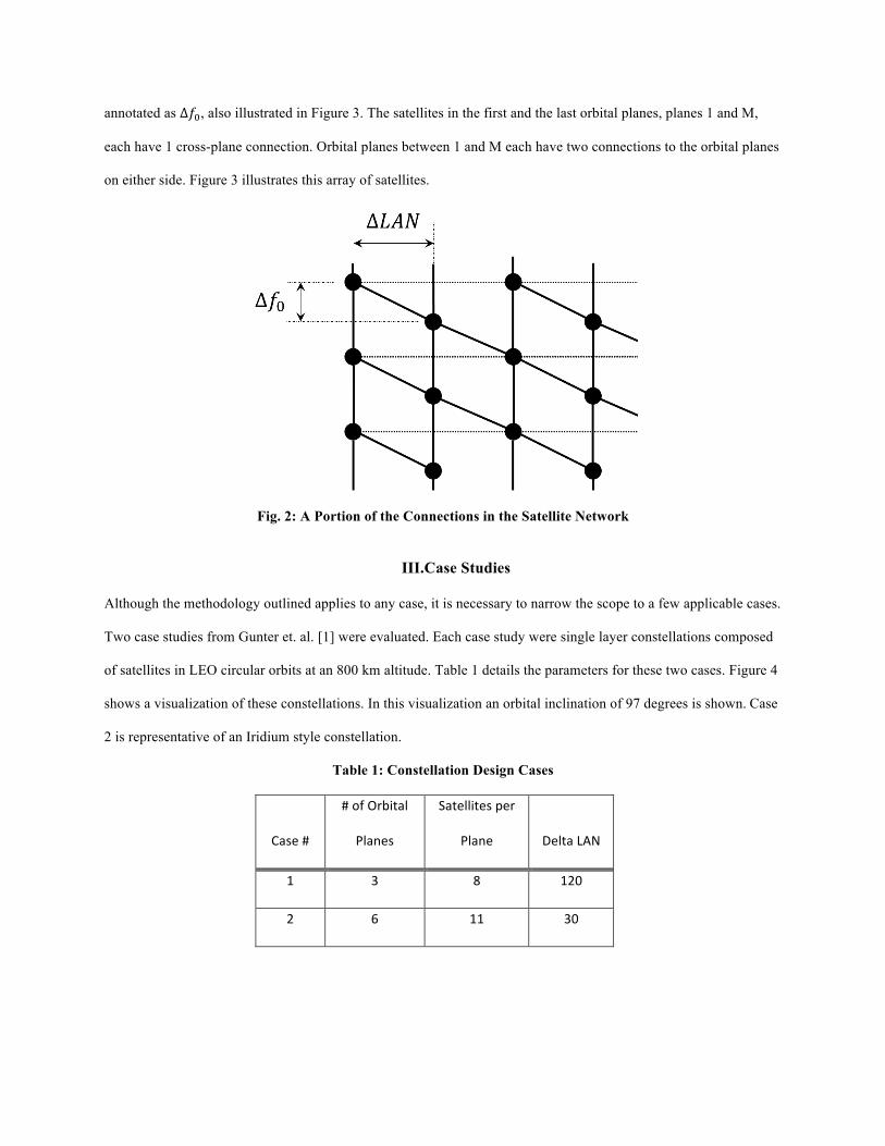
annotated as ∆𝑓!, also illustrated in Figure 3. The satellites in the first and the last orbital planes, planes 1 and M,

each have 1 cross-plane connection. Orbital planes between 1 and M each have two connections to the orbital planes

on either side. Figure 3 illustrates this array of satellites.

Fig. 2: A Portion of the Connections in the Satellite Network

III.Case Studies

Although the methodology outlined applies to any case, it is necessary to narrow the scope to a few applicable cases.

Two case studies from Gunter et. al. [1] were evaluated. Each case study were single layer constellations composed

of satellites in LEO circular orbits at an 800 km altitude. Table 1 details the parameters for these two cases. Figure 4

shows a visualization of these constellations. In this visualization an orbital inclination of 97 degrees is shown. Case

2 is representative of an Iridium style constellation.

Table 1: Constellation Design Cases

 

Case  #  

#  of  Orbital  

Planes  

Satellites  per  

Plane   Delta  LAN  

1   3   8   120  

2   6   11   30  

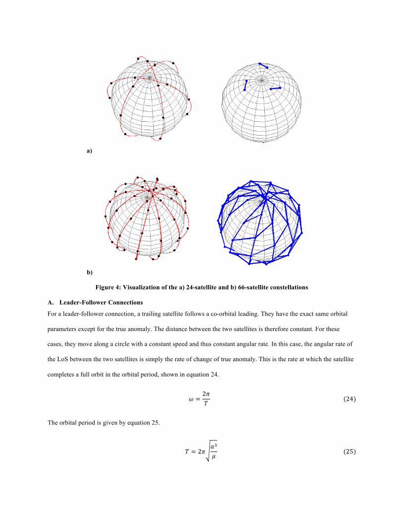
a)

b)

Figure 4: Visualization of the a) 24-satellite and b) 66-satellite constellations

A. Leader-Follower Connections

For a leader-follower connection, a trailing satellite follows a co-orbital leading. They have the exact same orbital

parameters except for the true anomaly. The distance between the two satellites is therefore constant. For these

cases, they move along a circle with a constant speed and thus constant angular rate. In this case, the angular rate of

the LoS between the two satellites is simply the rate of change of true anomaly. This is the rate at which the satellite

completes a full orbit in the orbital period, shown in equation 24.

𝜔 =2𝜋𝑇                                                                                                                                                                                      (24)

The orbital period is given by equation 25.

𝑇 = 2𝜋𝑎!

𝜇                                                                                                                                                                            (25)

For a satellite orbiting Earth at an 800 km altitude, the angular rate of the line of sight is,

𝜔 =𝜇𝑎!

=398600 km! s!

6371km + 800km ! = 0.00104rads= 0.0596  deg/s

Because this angular velocity is constant and in a constant direction, the angular acceleration is zero.

B. Cross Plane Connections

For each case evaluated, the distance and corresponding flux is evaluated for the duration of a pass, where a pair of

satellites experience closest approach. These results for flux are compared against a receiver sensitivity. By

observing where the reported flux crosses the sensitivity threshold, the connection time can be taken as the period in

which flux is above this threshold. Figures 5-12 show slew rate, angular acceleration, distance, and flux over the

duration of a pass. Figures 13-20 show the maximum slew rates, angular accelerations, and flux, and closest

approach for combinations of orbital inclination and offset of true anomaly.

Figure 5: Case 1, Slew Rate over Time for Various Orbital Inclinations

Figure 6: Case 1, Angular Acceleration over Time for Various Orbital Inclinations

Figure 7: Case 1, Distance over Time for Various Orbital Inclinations

Figure 8: Case 1, Flux over Time for Various Orbital Inclinations

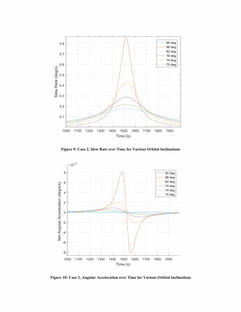
Figure 9: Case 2, Slew Rate over Time for Various Orbital Inclinations

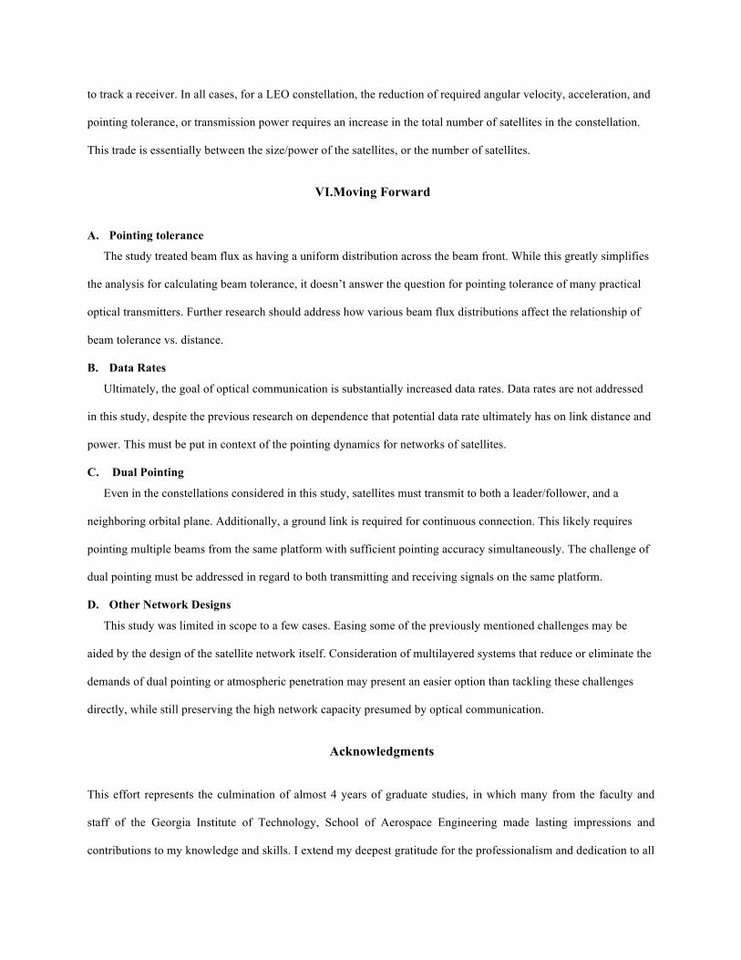
Figure 10: Case 2, Angular Acceleration over Time for Various Orbital Inclinations

Figure 11: Case 2, Distance over Time for Various Orbital Inclinations

Figure 12: Case 2, Flux over Time for Various Orbital Inclinations

Figure 13: Case 1, Closest Approach

Figure 14: Case 1, Peak Flux

Figure 15: Case 1, Peak Slew Rate

Figure 16: Case 2, Peak Angular Accelerations

Figure 17: Case 2, Closest Approach

Figure 18: Case 2, Max Flux

Figure 19: Case 2, Peak Slew Rate

Figure 20: Case 2, Peak Angular Acceleration

C. Downlinking Pointing

A network of satellites involves one or more ground terminals. This section aims to address feasibility of extending

optical communication to these receiving ground stations simply on the basis of pointing control. In practical

context, the distance and elevation at which connections can be established are affected by the atmosphere. The

analysis of downlinking is relatively simple in contrast to cross-linking, because in any case the satellites connecting

to a ground terminal moves at relatively the same speed of this ground terminal, and since all cases have the

satellites orbiting at the same, constant altitude, there will be little difference between each case. Granted the ground

station does move with the rotation of the earth. In this analysis, the only varied parameter is the downrange from

the passing satellite’s ground track, showed in figure 21.

Figure 21: Distance for various downrange angles

Figure 22: Flux for various downrange angles

Figure 23: Slew Rates for various downrange angles

Figure 24: Angular Acceleration for various downrange angles

IV.Discussion

This study evaluated a limited number of use cases all of which had the following similarities: single layer:

circular LEO; coorbital satellites were evenly distributed; all satellites had same inclination; difference in LAN of

orbital planes was constant until last orbital plane. These types of constellations are commonly used for networks of

communication satellites that often employ a large number of datalinks between antennas. Another assumption made

in the analysis is a uniform beam profile. This profile meant that the beam intensity was constant anywhere in the

beam at a given distance from the transmitter. This is not entirely accurate for most lasers, which often have beam

flux that tapers off gradually toward moving away from the boresight of the beam. The investigation on beam

tolerance did not address these types of non-uniform beam distributions. The study also did not address travel time

of the beam. The transmitted beam takes approximately 0.01 seconds to travel 3000, enough time for a receiver to

move by about 75 meters. This would need to be corrected for

This study focused primarily on the dynamics of the beam in slew rates and angular accelerations. It gave a

preliminary demonstration of the analysis techniques outlined in the methodology. The methodology gives general

expressions for the various parameters computed, including angular velocity and acceleration in vector form. The

benefit of these general expressions is that they can be further simplified for special cases, such as the ones in this

study, or they can be kept general for more complicated scenarios. The results of the case studies can then lead to

implications on necessary pointing control techniques and hardware, laying a trade-space for constellation and

satellite design.

Recall that a connection can only be established if the beam flux is above the sensitivity of the receiver.

This beam flux can be raised by adjusted the transmitter, or the sensitivity can be lowered (more sensitivity) by

adjusting the receiver. The case studies assumed the same transmitter and receiver as in Table 1. Case 2 results are

illustrated in Figure 8 and 12 and show that even if the closest approach for the cross-linked satellites is near

collision, the time for connection is at most 100 seconds. Figures 14 and 18 show that the constellation design is

somewhat constrained in order to have even brief moments of cross-plane connectivity. Additionally, the constraint

that these must be within 220 km for connection means that the 4000 km distance between the Iridium style

constellation (case 2) cannot establish leader-follower connections for this set of transmitter and receiver. This is the

least demanding of the cases. This means the transmitter and the receiver are not sufficiently powerful and sensitive

respectively for either constellation design. Recalling equation 8 and holding all other parameters constant, in order

for a leader-follower connection to be possible, the transmitter power must be 330 times higher, at roughly 1 kW.

A potential constellation concept could involve cross-plane connections that only occur at the poles. However,

the link distance for leader-follower connections must be short enough for sustained connection through the entire

orbital plane. If it is insisted that the optics for these links stay the same as in Table 1, this requires the entire length

of the 45,000 km circumference orbit have satellites equally spaced less than 220 kms. This subsequently requires a

minimum of 205 satellites per orbital plane. For constellations of small satellites, this may be reasonable. These are

in fact the cases in which power or receiver aperture may be constrained in size. This illuminates a trade-off between

satellite size/power and number satellites per orbital plane.

Examining the implications on pointing control, Figures 5 and 9 show the angular velocity over time for Case 1

and 2 respectively. Figures 6 and 10 show angular acceleration over time for Case 1 and 2 respectively. To

determine the maximum required slew rate and accelerations, refer to 15 and 16 for case 1 and 19 and 20 for case

two. A direct correlation between maximum slew rate and acceleration should be noted. Easing one requirement also

eases the other. It should also be noted that essentially, the only difference between case 1 and case 2 from the

requirements perspective for cross-plane links is the ∆𝐿𝐴𝑁. In comparing figure 15 (a case in which and 19, the a

shorter ∆𝐿𝐴𝑁 eases the requirements for slew rate and angular acceleration at the cost of more orbital planes. The

closeness of the neighboring planes also assists link margin by reducing the link distance. So it is clear that

increasing the number of orbital planes reduces every pointing requirement examined in the case study. It is clear

from this that relaxing the requirement for pointing control and link distance requires a substantial increase in the

number of satellites in the constellation.

A lingering question is what the technical possibility of maintaining pointing accuracy is. One provider of

CubeSat buses and attitude control systems is Blue Canyon Technologies. Their XACT integrated attitude control

system provides a pointing accuracy of 0.003 degrees, well below the 1 mrad (or 0.057 degrees) pointing tolerance

required in the trade studies [6]. It also produces a slew rate of over 10 deg/sec as well as providing torque and

momentum specifications for various reaction control wheels. However, it is not clear that the system can maintain

this pointing accuracy while also maintaining the slew rate, which is what is required for these optical links.

V.Conclusion

This study examined the pointing requirements of optical (laser) communications for networks of satellites. For

these optical connections, tolerance of pointing accuracy, angular velocity, and angular acceleration were quantified

for 2 different cases over the time frame of closest approach, with varying degrees of orbital inclination and anomaly

offsets. Two distinct categories of links were identified for these cases: leader-follower, and cross-plane. Leader-

follower connections were found to have little demand on angular velocity and angular acceleration due to their

constant angular velocity. This means that satellites within the same orbital plane and within required distances are

arguably the simplest feasible connection for satellite crosslinking of optical connections. Connecting one satellite to

another in a different orbital plane presented a challenge for the actuation of beam orientation due to varying slew

rates required to maintain pointing tolerance, though it was demonstrated how various constellation design

parameters can relax the requirements for these pointing dynamics. A preliminary examination of available CubeSat

attitude control systems showed the technology for these pointing requirements is already commercially available.

Though it still needs to be determined if the required pointing tolerance can be maintained while a transmitter slews

to track a receiver. In all cases, for a LEO constellation, the reduction of required angular velocity, acceleration, and

pointing tolerance, or transmission power requires an increase in the total number of satellites in the constellation.

This trade is essentially between the size/power of the satellites, or the number of satellites.

VI.Moving Forward

A. Pointing tolerance

The study treated beam flux as having a uniform distribution across the beam front. While this greatly simplifies

the analysis for calculating beam tolerance, it doesn’t answer the question for pointing tolerance of many practical

optical transmitters. Further research should address how various beam flux distributions affect the relationship of

beam tolerance vs. distance.

B. Data Rates

Ultimately, the goal of optical communication is substantially increased data rates. Data rates are not addressed

in this study, despite the previous research on dependence that potential data rate ultimately has on link distance and

power. This must be put in context of the pointing dynamics for networks of satellites.

C. Dual Pointing

Even in the constellations considered in this study, satellites must transmit to both a leader/follower, and a

neighboring orbital plane. Additionally, a ground link is required for continuous connection. This likely requires

pointing multiple beams from the same platform with sufficient pointing accuracy simultaneously. The challenge of

dual pointing must be addressed in regard to both transmitting and receiving signals on the same platform.

D. Other Network Designs

This study was limited in scope to a few cases. Easing some of the previously mentioned challenges may be

aided by the design of the satellite network itself. Consideration of multilayered systems that reduce or eliminate the

demands of dual pointing or atmospheric penetration may present an easier option than tackling these challenges

directly, while still preserving the high network capacity presumed by optical communication.

Acknowledgments

This effort represents the culmination of almost 4 years of graduate studies, in which many from the faculty and

staff of the Georgia Institute of Technology, School of Aerospace Engineering made lasting impressions and

contributions to my knowledge and skills. I extend my deepest gratitude for the professionalism and dedication to all

in the Institute who helped to make my MSAE a reality. I thank my advisor, Dr. Brian Gunter for his guidance over

the course of this research and for introducing me to the fascinating concepts explored with small satellites and

Lasercomm.

References

[1] Gunter, B. C., and Maessen, D. C., “Space-Based Distributed Computing Using a Networked Constellation of Small

Satellites,” Journal of Spacecraft and Rockets, September 2013

[2] Panahi, A., and Kazemi, A. A., “Optical Laser Cross-Link in Space-Based Systems used for Satellite Communications,”

presented at SPIE, 5 Apr 2010

[3] Noble, L.A., “Dual Fine Tracking Control of a Satellite Laser Communication Uplink,” M.S. Thesis, Aeronotics and

Astronautics Dept, Air Force Institute of Technology, Wright-Patterson AFB, OH, 2006.

[4] Dunbar, B., and Mohon, L., “Laser Communications Relay Demonstration (LCDR) Overview,” NASA Mission Pages [online

archive], URL: https://www.nasa.gov/mission_pages/tdm/lcrd/overview.html, retrieved 4 August 2017.

[5] Sburlan, S., and Kueppers, M., “Introduction to Optical Communications for Satellites,” Presented at Keck Institute for Space

Studies, 11 July 2016.

[6] Blue Canyon Technologies Incorporated, bluecanyontech.com, data retrieved 4 August 2017