An Evaluation of Dvorak Technique–Based Tropical Cyclone ... · An Evaluation of Dvorak...
18
An Evaluation of Dvorak Technique–Based Tropical Cyclone Intensity Estimates JOHN A. KNAFF NOAA/NESDIS/Regional and Mesoscale Meteorology Branch, Fort Collins, Colorado DANIEL P. BROWN NOAA/NWS/National Hurricane Center, Miami, Florida JOE COURTNEY Bureau of Meteorology, Perth, Western Australia, Australia GREGORY M. GALLINA NOAA/NESDIS/Satellite Analysis Branch, Camp Springs, Maryland JOHN L. BEVEN II NOAA/NWS/National Hurricane Center, Miami, Florida (Manuscript received 28 October 2009, in final form 1 April 2010) ABSTRACT The satellite-based Dvorak technique (DVKT) is the most widely available and readily used tool for op- erationally estimating the maximum wind speeds associated with tropical cyclones. The DVKT itself produces internally consistent results, is reproducible, and has shown practical accuracy given the high cost of in situ or airborne observations. For these reasons, the DVKT has been used in a reasonably uniform manner globally for approximately 20 years. Despite the nearly universal use of this technique, relatively few systematic verifications of the DVKT have been conducted. This study, which makes use of 20 yr of subjectively de- termined DVKT-based intensity estimates and best-track intensity estimates influenced by aircraft observations (i.e., 62 h) in the Atlantic basin, seeks to 1) identify the factors (intensity, intensity trends, radius of outer closed isobar, storm speed, and latitude) that bias the DVKT-based intensity estimates, 2) quantify those biases as well as the general error characteristics associated with this technique, and 3) provide guidance for better use of the operational DVKT intensity estimates. Results show that the biases associated with the DVKT-based intensity estimates are a function of intensity (i.e., maximum sustained wind speed), 12-h intensity trend, latitude, and translation speed and size measured by the radius of the outer closed isobar. Root-mean-square errors (RMSE), however, are shown to be primarily a function of intensity, with the best signal-to-noise (intensity to RMSE) ratio occurring in an intensity range of 90–125 kt (46–64 m s 21 ). The knowledge of how these factors affect intensity estimates, which is quantified in this paper, can be used to better calibrate Dvorak intensity estimates for tropical cyclone forecast operations, postseason best-track analysis, and climatological reanalysis efforts. As a demonstration of this capability, the bias corrections developed in the Atlantic basin are also tested using a limited east Pacific basin sample, showing that biases and errors can be significantly reduced. 1. Introduction The Dvorak technique (DVKT), which estimates the intensity of tropical cyclones (TCs) by analyzing satellite image patterns (Dvorak 1972, 1975, 1984) and infrared cloud-top temperatures (Dvorak 1984, 1995), has become an important operational tool over the last 30 years (Velden et al. 2006a). The DVKT assigns an intensity estimate in terms of intensity units or ‘‘T numbers,’’ which range from 1 to 8 in increments of 0.5 where a unit T number was designed to correspond to the climato- logical rate of tropical cyclone intensification. Corresponding author address: John Knaff, NOAA/NESDIS/ RAMMB, Colorado State University, CIRA, Foothills Campus Delivery 1375, Fort Collins, CO 80523-1375. E-mail: [email protected] 1362 WEATHER AND FORECASTING VOLUME 25 DOI: 10.1175/2010WAF2222375.1
Transcript of An Evaluation of Dvorak Technique–Based Tropical Cyclone ... · An Evaluation of Dvorak...

An Evaluation of Dvorak Technique–Based Tropical Cyclone Intensity Estimates
JOHN A. KNAFF
NOAA/NESDIS/Regional and Mesoscale Meteorology Branch, Fort Collins, Colorado
DANIEL P. BROWN
NOAA/NWS/National Hurricane Center, Miami, Florida
JOE COURTNEY
Bureau of Meteorology, Perth, Western Australia, Australia
GREGORY M. GALLINA
NOAA/NESDIS/Satellite Analysis Branch, Camp Springs, Maryland
JOHN L. BEVEN II
NOAA/NWS/National Hurricane Center, Miami, Florida
(Manuscript received 28 October 2009, in final form 1 April 2010)
ABSTRACT
The satellite-based Dvorak technique (DVKT) is the most widely available and readily used tool for op-
erationally estimating the maximum wind speeds associated with tropical cyclones. The DVKT itself produces
internally consistent results, is reproducible, and has shown practical accuracy given the high cost of in situ or
airborne observations. For these reasons, the DVKT has been used in a reasonably uniform manner globally
for approximately 20 years. Despite the nearly universal use of this technique, relatively few systematic
verifications of the DVKT have been conducted. This study, which makes use of 20 yr of subjectively de-
termined DVKT-based intensity estimates and best-track intensity estimates influenced by aircraft observations
(i.e., 62 h) in the Atlantic basin, seeks to 1) identify the factors (intensity, intensity trends, radius of outer closed
isobar, storm speed, and latitude) that bias the DVKT-based intensity estimates, 2) quantify those biases as well
as the general error characteristics associated with this technique, and 3) provide guidance for better use of the
operational DVKT intensity estimates. Results show that the biases associated with the DVKT-based intensity
estimates are a function of intensity (i.e., maximum sustained wind speed), 12-h intensity trend, latitude, and
translation speed and size measured by the radius of the outer closed isobar. Root-mean-square errors (RMSE),
however, are shown to be primarily a function of intensity, with the best signal-to-noise (intensity to RMSE)
ratio occurring in an intensity range of 90–125 kt (46–64 m s21). The knowledge of how these factors affect
intensity estimates, which is quantified in this paper, can be used to better calibrate Dvorak intensity estimates
for tropical cyclone forecast operations, postseason best-track analysis, and climatological reanalysis efforts. As
a demonstration of this capability, the bias corrections developed in the Atlantic basin are also tested using
a limited east Pacific basin sample, showing that biases and errors can be significantly reduced.
1. Introduction
The Dvorak technique (DVKT), which estimates the
intensity of tropical cyclones (TCs) by analyzing satellite
image patterns (Dvorak 1972, 1975, 1984) and infrared
cloud-top temperatures (Dvorak 1984, 1995), has become
an important operational tool over the last 30 years
(Velden et al. 2006a). The DVKT assigns an intensity
estimate in terms of intensity units or ‘‘T numbers,’’
which range from 1 to 8 in increments of 0.5 where a unit
T number was designed to correspond to the climato-
logical rate of tropical cyclone intensification.
Corresponding author address: John Knaff, NOAA/NESDIS/
RAMMB, Colorado State University, CIRA, Foothills Campus
Delivery 1375, Fort Collins, CO 80523-1375.
E-mail: [email protected]
1362 W E A T H E R A N D F O R E C A S T I N G VOLUME 25
DOI: 10.1175/2010WAF2222375.1

Without going into great detail, the method involves
locating the storm center, assigning a pattern (e.g., eye,
shear, banded, central dense overcast, etc.), making mea-
surements from satellite imagery (visible or enhanced in-
frared), assigning a T number, and estimating the current
intensity (CI) by following the rules or constraints speci-
fied by the technique. The visible and enhanced IR (EIR)
techniques also provide similar results [i.e., 95% were
within a half T number; Gaby et al. (1980)]. The CI then
corresponds to a maximum wind speed, as show in Table 1,
which comes from Dvorak (1984). Other CI versus max-
imum wind speed/minimum sea level pressure (MSLP)
tables have also been developed for use at other World
Meteorological Organization (WMO) Regional Special-
ized Meteorological Centres (RSMCs) and Australian
Tropical Cyclone Warning Centres (TCWCs) to account
for different wind-averaging periods and wind–pressure
relationships. For more information on wind–pressure
relationships, see Koba et al. (1990, 1991), Knaff and
Zehr (2007, 2008), Courtney and Knaff (2009), Holland
(2008), and Harper (2002). It should also be noted that
users of the DVKT in other basins have also applied
regional variations and modifications (Velden et al.
2006b) to the DVKT as described in Dvorak (1984).
Throughout the late 1980s and 1990s, there was a
concerted WMO training effort to educate forecasters in
the use of proven/standard techniques for tropical cyclone
forecasting, including the Dvorak technique (WMO
2000). As a result of this effort, most WMO RSMCs and
TCWCs were using the Dvorak technique in operations
by the late 1980s (Harper et al. 2008; Velden et al.
2006a). The DVKT has been shown to be relatively
stable with respect to satellite sensor resolution (Zehr
et al. 2010). The DVKT has also been shown to be re-
producible and internally consistent [i.e., different ana-
lysts using the same imagery produce roughly the same
results; Guard (1988); Mayfield et al. (1988)]. Guard
(1988) found that 54% and 82% of 87 of the more difficult
1986 western North Pacific cases were within 60.5 and
61.0, respectively, T numbers when analysts were
shielded from operational information. Mayfield et al.
(1988) examined the reliability of DVKT estimates by
using as many as 14 analysts in a controlled study of
eastern Pacific tropical cyclones to produce dispersion
statistics associated with the DVKT; finding standard
deviations from the consensus average of 4.3, 9.0, 10.7,
and 12.0 kt for tropical depressions, tropical storms,
hurricanes with intensities of 65–95 kt (33–49 m s21;
1 kt 5 0.514 m s21), and hurricanes with intensities greater
than 95 kt, respectively. Historical records of DVKT-
based intensity estimates also exist, which represents
a quality global climate record of tropical cyclone in-
tensity (e.g., Sampson and Schrader 2000; Nakazawa
and Hoshino 2009). However, few systematic, multiyear
validations of these estimates versus aircraft reconnais-
sance estimated/influenced maximum surface winds es-
timates (i.e., via best track when aircraft reconnaissance is
available) have been performed. One such study (Sheets
and McAdie 1988) examined the error distribution based
on best-track intensities with aircraft reconnaissance
within 6 h of the DVKT estimate in the Atlantic basin.
Sheets and McAdie (1988) found biases of 2.1, 23.5,
and 23.2 kt and RMS errors of 5.7, 8.0, and 13.2 kt for
the tropical depression, tropical storm, and hurricane
cases, respectively. This paper will conduct a similar,
yet more comprehensive, study.
The purpose of this verification is to document error
characteristics and possible systematic biases associated
with the use of the DVKT. Specifically we seek to answer
the following questions: How accurate is the DVKT?
Does the DVKT have systematic biases? Are there sys-
tematic differences between estimates made at different
agencies? Can the DVKT be better calibrated by using
conditional information available in the operational
setting?
Previous studies have documented DVKT biases and
errors as functions of intensity (Sheets and McAdie 1988),
latitude (Kossin and Velden 2004), and intensification
trend (Koba et al. 1990, 1991; Brown and Franklin 2002,
2004). Several authors have also mentioned that the
DVKT assumes a climatological translation speed (e.g.,
Velden et al. 2006a; Courtney and Knaff 2009; Harper
2002; Harper et al. 2008). In addition to latitude and
intensification trends, biases and errors will be quantified
as a function of intensity, size in terms of the radius of the
outer closed isobar (ROCI), and storm translation speed.
TABLE 1. The lookup table for Dvorak CI vs tropical cyclone
maximum wind speed from Dvorak (1984). Wind speeds are valid
for 1-min maximum sustained winds at a 10-m elevation and
a marine exposure and are given in knots (kt).
Dvorak CI Max wind speed (kt)
1.0 25
1.5 25
2.0 30
2.5 35
3.0 45
3.5 55
4.0 65
4.5 77
5.0 90
5.5 102
6.0 115
6.5 127
7.0 140
7.5 155
8.0 170
OCTOBER 2010 K N A F F E T A L . 1363
Those results will then be used to create a conditional
calibration of DVKT intensity estimates that may be
useful in operations as well as for climatological rean-
alyzes. The following sections describe the datasets used
in this study, details about how the verification was con-
ducted, results of the verification, and a description of the
resulting calibration method. The final section will sum-
marize the important results and discuss their implica-
tions for climatological tropical cyclone reanalysis and
operational tropical cyclone forecasting.
2. Datasets
All of the datasets used in this study come from the
databases of the Automated Tropical Cyclone Forecast
(ATCF; Sampson and Schrader 2000) system. This study
makes use of all tropical cyclones occurring from 08 to
1408W longitude during the years 1989–2008. The Atlantic
basin sample is used as a dependent sample and the east
Pacific is used as an independent sample. Specifically, the
intensity estimates used for verification come from the best
tracks (i.e., B decks). The Dvorak intensity estimates, from
the National Environmental Satellite, Data, and Informa-
tion Service’s (NESDIS) Satellite Analysis Branch (SAB)
and the Tropical Analysis and Forecast Branch (TAFB),
which is part of the Tropical Prediction Center/National
Hurricane Center, and aircraft reconnaissance fixes come
from the fix file (i.e., F deck). Since it was also desirable to
examine the effects of TC size, the radius of the outer
closed isobar (ROCI) was provided in the objective aid file
(A deck). The ROCI values are not available in the best
track, prior to 2004, so ROCI estimates are taken from the
A deck, which is the same procedure used in
the ‘‘extended best track’’ (Kimball and Mulekar 2004;
Demuth et al. 2006). ROCI is not reevaluated following
the season as is the track and intensity and, thus, is likely of
lower quality. Since the native units for intensity are knots,
or nautical miles per hour, and for ROCI are nautical
miles (n mi, where 1 n mi 5 1.85 km), these units will
be used throughout the remainder of the manuscript.
There are also a few modifications to the fix files that
were necessary to properly complete this study. The fix
files were modified in the following ways for use with the
software developed for this study: 1) intensities for the
Dvorak fixes were added to the files in 2002 using the CI
to intensity table (CI was in the fix files); 2) if the aircraft
fixes reported a minimum sea level pressure and a maxi-
mum wind estimate, an ‘‘I’’ (i.e., as an intensity fix) was
added to the fix identifier in 2002; 3) all references to the
site KSAB were changed to SAB in 1989; and 4) all the
fixes from the National Hurricane Center in Miami,
Florida [i.e., those from the Tropical Satellite Analysis
Center (TSAC), Tropical Satellite Analysis and Forecast
(TSAF) unit, and TAFB] are treated as coming from
TAFB, and references to TSAC and TSAF were changed
to TAFB. None of these changes introduced intensity
information not already included in the individual fixes,
but allowed for a longer homogeneous record by cor-
recting inconsistencies in the file format and errors
introduced by different operational procedures and
software.
Since the rules or ‘‘constraints’’ of the DVKT limit the
rate of change of the DVKT intensity estimates, the timing
of the first DVKT intensity classification can be important
in determining the final DVKT intensity estimate or CI.
For this reason, this study will also examine the timing of
the initial fix times for each of the two agencies. This was
accomplished by examining all of the DVKT-based in-
tensity fixes from SAB and TAFB, with and without air-
craft reconnaissance, in the same 08–1408W domain and
years.
One could also argue that once an aircraft intensity
estimate has been obtained, the estimate influences sub-
sequent DVKT- based intensity estimates. To examine
the possible influence of aircraft-based fixes on subse-
quent DVKT intensity estimates, this study will also ex-
amine biases with respect to intensity associated with
DVKT intensity fixes that coincide or proceeded the time
of the first aircraft MSLP estimate/fix on a tropical
cyclone.
Infrared imagery archives maintained at the Cooper-
ative Institute for Research in the Atmosphere (CIRA;
Zehr and Knaff 2007) and the NHC are also examined to
interpret the DVKT validation results. It should be men-
tioned that both of these datasets have reduced precision
when compared to the raw Geostationary Operational
Environmental Satellite (GOES) data. The CIRA archive
has 8-bit resolution (256 counts) and the NHC archive has
7-bit resolution (128 counts). Despite these differences,
the calibration at colder temperatures is the same for the
CIRA and NHC archives. GOES imagery has 10-bit
precision (1024 counts). The use of 7-bit data in opera-
tions, however, results in a random (rather than a system-
atic) cloud-top enhancement differences. This reduction
in precision will occasionally change the interpretation
of individual cases if 10- or 8-bit GOES data are en-
hanced and the EIR technique applied.
3. Methodology
A homogeneous verification of the DVKT-based in-
tensity estimates is constructed using a time window of
62 h of a best-track time. The verification was based
upon periods that the best-track intensity was influenced
by a reconnaissance fix (i.e., within 62 h) and the
DVKT fixes were also within the same time window. For
1364 W E A T H E R A N D F O R E C A S T I N G VOLUME 25
each DVKT-based intensity fix, the best-track intensity
is interpolated to the time of that individual fix obser-
vation. From these individual verification points the
biases and errors associated with the fixes are calculated.
The verifications are further stratified by intensity and
latitude, storm speed, intensity trend, and ROCI in com-
bination with intensity. Statistics associated with the er-
rors and biases, as well as the stratification factors, are
compiled for each verification subset. Figure 1 shows the
best-track locations of the homogeneous fixes used in this
study. The reader should notice the reliance on aircraft
results in relatively few fixes west (east) of 1108W (608W)
and equatorward (poleward) of 128N (408N). For this
study we will initially concentrate on intensity estimates
made in the Atlantic basin and then apply the Atlantic
results to a much smaller sample of east Pacific cases. This
stratification in the Atlantic resulted in a sample of 2003
cases, of which 6.0%, 43.7%, 31.1%, and 19.2% were
tropical depressions, tropical storms, minor hurricanes,
and major hurricanes, respectively. Similarly, there were
49 cases in the east Pacific, of which 0.0%, 30.6%, 38.7%,
and 30.6% were tropical depressions, tropical storms,
minor hurricanes, and major hurricanes, respectively.
The fact that these distributions vary from climatology
will be addressed by binning classifications to equalize
their influences on subsequently presented statistics.
Since the timing of the first DVTK intensity estimate
is potentially important in the determination of the DVKT
intensity estimation or CI because the constraints limit the
rate of intensification to 2.5 T numbers per day, statistics
concerning the time differences between the first fix made
by each agency were also compiled based on the combi-
nation of all fixes in both basins. These statistics are then
used to examine the possible effects of first classification
timing differences on interagency intensity estimation
differences.
To examine the potential impacts of aircraft-based
intensity estimates on subsequent DVKT intensity esti-
mates, best-track times were identified that were influ-
enced by aircraft fixes, but the DVKT intensity estimates
near those best-track times were created coincidently or
after the first aircraft estimate of MSLP was observed.
For this limited analysis the DVKT intensity estimates
from both agencies had to be made coincidently or be-
fore, but within 2 h of when the first aircraft-based in-
tensity estimate was available. Presumably, the DVKT
fixes from these cases will not benefit from knowing the
observed intensity of the storm at any prior time and thus
are more independent.
4. Results
a. Interannual statistics
The interannual variations of the DVKT intensity
estimates are first examined to see if known changes in
technology have affected the bias and error character-
istics of the DVKT-based intensity estimates. Examples
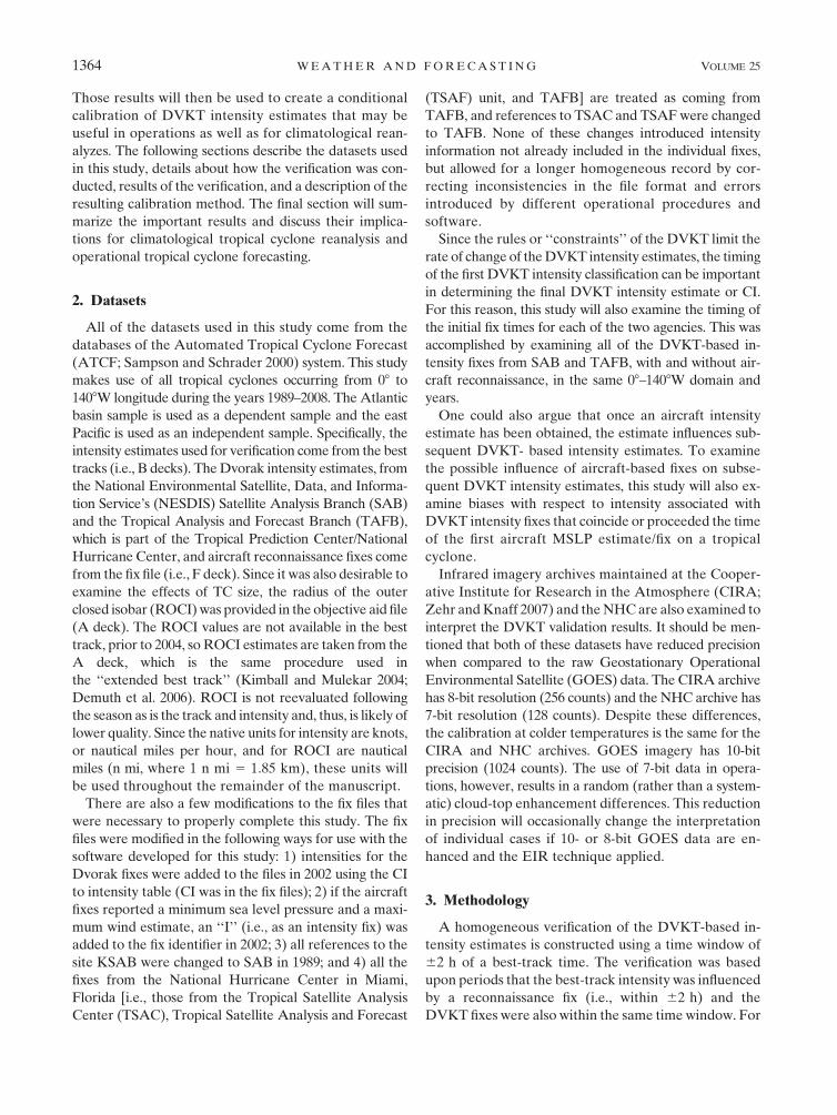
FIG. 1. A map showing the locations of the homogeneous verification points whose best-track
intensities were influenced (within 62 h) by aircraft reconnaissance used in this study. The
black and gray hurricane symbols indicate that the best-track intensity was greater than or
equal to the hurricane strength and less than the hurricane strength, respectively, for that
verification point. Points in the Atlantic basin are used to examine biases and errors associated
with the DVKT and points in the east Pacific are used as an independent dataset to test the
results found in the Atlantic sample.
OCTOBER 2010 K N A F F E T A L . 1365

of such changes include satellite coverage and resolution1
changes in the analysis domain and viewing angles with
the introduction of GOES-8 in 1995 and GOES-9 in 1997,
which replaced GOES-7, which was located in a central
location (1058W). Other factors include the impacts of
changes in flight-level to surface wind reductions based
on GPS dropwindsonde analyses that started in approx-
imately 2000 [and that are documented in Franklin et al.
(2003)] might have had on operational and best-track
intensity estimates. There were also potential procedural
differences that occurred during this time period, such as
the treatment of weakening systems (i.e., Brown and
Franklin 2004)2 and the Dvorak (1995) notes on the shear
pattern.
Figure 2 shows the interannual variations of biases,
mean absolute error (MAE), and root-mean-square error
(RMSE) of the 2003 Atlantic DVKT cases. There is a
tendency for TAFB’s estimates to be slightly higher than
SAB’s estimates. These differences have diminished
since 2002. One would expect technological (e.g., satellite
resolution and viewing angles, dropwindsondes) and
procedural changes (e.g., flight-level to surface reduction)
to effect the performance of both agencies. However,
there do not seem to be any visually detectable change
points associated with known changes in operational
procedures or technology. There is however a slight
upward trend in errors in the TAFB fixes that explains
about 13% of the variance, which does not seem to be
associated with any of the changes in technology and may
reflect other internal changes. No statistically significant
trends were found in the MAE or RMSE statistics. There
is also a fair amount of interannual variance in the biases
and errors, but the statistics from the two agencies seem
to have a reasonable covariance. The DVKT is also
shown to be much more reproducible than in the Guard
(1988) study, with 95% and 55% of the SAB and TAFB
fixes being within 60.5 T number and equal, respectively,
for the 2003-case Atlantic sample. Average MAEs and
RMSEs are also remarkably stable during 1989–2008, with
mean values of approximately 8 and 11 kt, respectively.
Note here that the Guard (1988) study purposely exam-
ined the 87 most difficult cases and was likely more
shielded from the intensity information coming from air-
craft. The lack of coincident change points,3 particularly in
the MAE and RMSE, provides confidence that the entire
1989–2008 time period can be treated as quasi-stationary
and can be examined in a homogeneous manner. This
assumption is further supported by the interagency cor-
relation coefficients of 0.81, 0.48, and 0.48 for biases,
MAEs and RMSEs, respectively, and the detrending of
these datasets did not change these correlations. These
calculations suggest that there are likely systematic,
rather than random, causes for the interannual variations
that affect the DVKT performance at both agencies that
have remained consistent throughout the time of analysis.
The assumption of quasi-stationary also allows for the
more thorough examination of potential conditional biases
FIG. 2. Time series of the (top) interannual variability of biases,
(middle) MAEs, and (bottom) RMSEs associated with the Dvorak
tropical cyclone intensity estimation technique. Statistics are based
on a homogeneous comparison between fixes made at SAB and
TAFB that were made within 62 h of an aircraft reconnaissance fix
and have units of knots. The verification is based on best-track
intensity estimates at those times, and the analysis domain was the
Atlantic basin. The number of cases is provided in the bottom
panel.
1 The spatial resolutions of the visible and IR imagery are ap-
proximately 2 and 8 km for GOES-7 and 1 and 4 km for GOES-8
and GOES-9.2 While Brown and Franklin (2004) made recommendations on
how to improve the treatment of weakening systems, these rec-
ommendations were never formally adopted at SAB or TAFB.3 A rank-order change-point test was inconclusive; see Peterson
et al. (1998) for test details.
1366 W E A T H E R A N D F O R E C A S T I N G VOLUME 25

associated with the DVKT. To provide the reader with
additional information, many of the analyses that are
discussed in the following sections were performed on
the full 1989–2008 period and on the much shorter
2002–08 period; comments about the differences found
are provided.
b. Biases and errors as a function of intensity
The results of the homogeneous verification are
compiled in overlapping bins that have endpoints that
correspond to the CI versus intensity table shown in
Table 1. For instance, the first and second bins have best-
track intensity ranges of 20–35 and 25–45 kt, respec-
tively. Figure 3 shows the biases, MAEs, and RMSEs
associated with the DVKT-based intensity estimates.
Also shown in Fig. 3 is the number of cases in each bin.
The last bin extends from 127 to 170 kt because there
are limited numbers of cases with best-track intensities
greater than 140 kt. The biases, MAEs, and RMSEs
shown in Fig. 3 appear to be a function of intensity. The
biases show that the DVKT has a tendency to under-
estimate intensities when TCs have intensities between
35 and 55 kt and greater than 125 kt. On the other hand,
overestimation of intensities occurs for intensities between
75 and 105 kt. These results are mirrored in the shorter
2002–08 results (not shown), though the differences be-
tween SAB and TAFB are nearly zero above 80 kt; the
implications of which will be discussed in section 4e. The
low biases between 35 and 55 kt (CIs between 2.5 and
3.5) are consistent with those found by Sheets and
McAdie (1988), Koba et al. (1990, 1991), and Brown and
Franklin (2002). This issue likely resulted in Koba et al.
(1990, 1991) adjusting the CI versus intensity table used
at RSMC Tokyo, effectively increasing the intensities
for CI , 4.5. Independently, Brown and Franklin (2002)
suggested that DVKT rules limiting the rate of
strengthening of these weaker systems may be too re-
strictive. The high biases between 75 and 100 kt were
attributed to rules concerning a sometimes unrealistic
persistence of peak intensities in Brown and Franklin
(2002) and led Koba et al. (1990, 1991) earlier to de-
crease their intensities for CI . 5.0. Intensity estimates
in this range can also be obtained by using the embedded
center pattern, which is difficult to apply without accu-
rate center positions. Noteworthy for this discussion is
that the embedded eye pattern appears to give higher
than warranted intensity estimates when the embedded
center pattern is used after employing some other pat-
tern (Burton 2005). The low biases above approximately
125 kt were not apparent in the Brown and Franklin
(2002, 2004) or Koba studies, but in this study they were
primarily associated with several long-lived major
hurricanes (Ivan in 2004; Dennis, Emily, and Wilma in
2005; and Dean in 2007) that occurred since that time.
These results roughly agree with Sheets and McAdie
(1988), who found underestimation occurred for a rela-
tively large sample of hurricanes within 66 h of re-
connaissance.
MAEs and RMSE, also shown in Fig. 3, are lowest for
weak storms and largest for the higher intensities. The
errors associated with hurricanes and tropical storms in
this study, in general, are slightly smaller (;1 kt) than
those reported by Sheets and McAdie (1988). A possibly
better measure of the DVKT ability is the signal (in-
tensity) to noise (RMSE error) ratio. Using this metric,
the intensity estimate is most skillful–least in error in an
FIG. 3. (top) Biases, (middle) MAEs, and (bottom) RMSEs as-
sociated with Dvorak tropical cyclone intensity estimates (kt) from
SAB and TAFB that were made with 62 h of an aircraft re-
connaissance fix. The verification is based on the best-track in-
tensities at those times, and the analysis domain was the Atlantic
basin. The number of cases is provided in the bottom panel.
OCTOBER 2010 K N A F F E T A L . 1367
intensity range from approximately 90 to 125 kt (i.e., CIs
of from 5.0 to 6.5), where signal to noise ratios are greater
than 7. This is likely due to the existence of the relatively
stable ‘‘eye’’ pattern that exists in these intensity ranges;
therefore, the technique is more objective in this range. It
also appears that the method has more difficulty in esti-
mating the intensities of weaker tropical cyclones, where
the signal-to-noise ratio has a value between 5 and 6. At
these lower intensities, there can be multiple DVKT
patterns associated with a given intensity estimate and
the centers of these systems are often more difficult to
locate. Somewhat surprising are the errors that result
from large negative biases at the highest intensity ranges
that suggest that above ;125 kt there is less skill in dis-
criminating the stronger category 4 (114–135 kt) from
category 5 (.135 kt) storms. Possible reasons for these
findings include the following. 1) Because the climato-
logical tropopause temperature in the Atlantic is about
2768C, it is more difficult for convection to produce a
complete ring of cloud tops 2768C or colder with a
minimum width requirement of 55 km. This type of pat-
tern is generally required for intensity estimates of 6.5 T
numbers or greater using the EIR method. 2) Smaller
very intense storms are likely underestimated due to not
having a cold ring of convection surrounding the eye that
meets the minimum width requirement in the EIR tech-
nique. 3) There is an inability in some cases to resolve the
warm eye temperatures that occur with very small eyes
or ‘‘pinhole eyes’’ or at steep satellite viewing angles.
4) Dvorak constraints can be too restrictive for rapidly
intensifying storms. 5) There is no explicit treatment of
concentric multiple eyewalls and there are no explicit
rules that apply to eyewall replacement cycles. These
potential shortcomings will be discussed further in sec-
tion 4e. The results discussed above are not significantly
different from the results obtained using the 2002–08 time
period, though the differences corresponding to near-
hurricane intensity between the SAB and TAFB errors
are reduced (not shown).
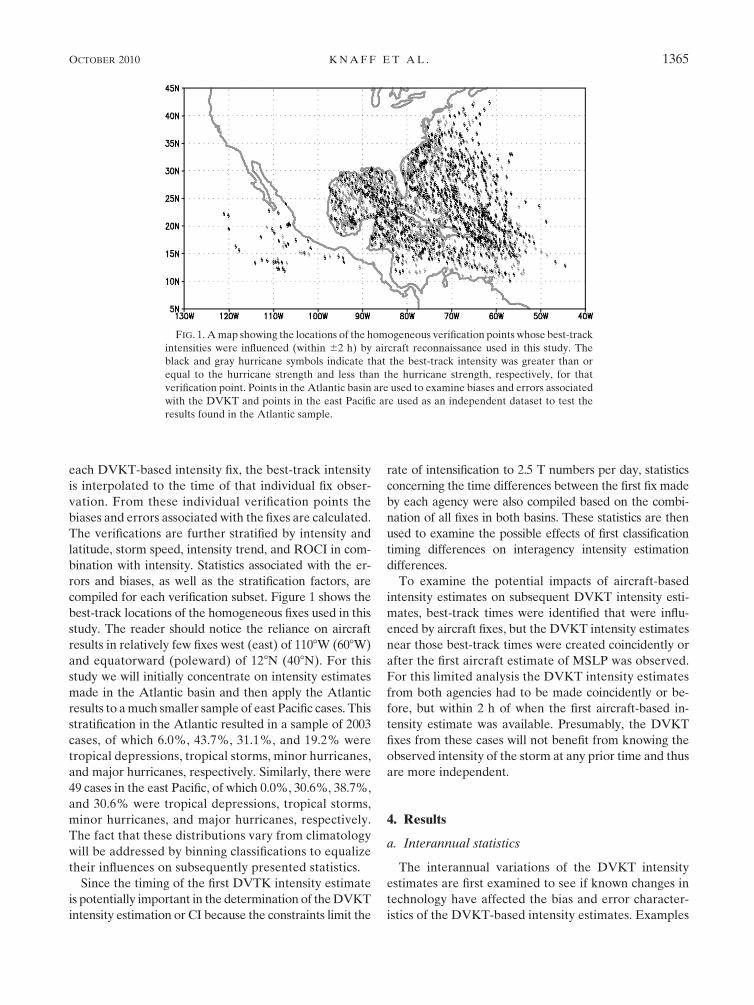
Since the precision of the DVKT CI versus intensity
table (i.e., Table 1) is itself a function of intensity, it is
worth calculating the RMSEs in terms of DVKT T num-
bers as a function of CI. This comparison is shown in Fig. 4.
It appears that the DVKT was designed to have RMSEs
of roughly 0.5 T number. This transformation does not
change the results shown in Fig. 3 and still shows that the
relative errors are larger for weak and very strong storms
with a relative ‘‘sweet spot’’ for intensity estimation for
CI ranging from 5.0 to 6.5. However, it also suggests that
the signal-to-noise ratio in terms of T numbers is roughly
increasing linearly from a low of ;4 at CI 5 2.0 to a high
near ;14 at CI 5 7.0. This transformation also highlights
the larger TAFB errors for CIs of 4.0 and 4.5, which are
largely attributed to overestimation or high bias in this
intensity range.
c. Influences of aircraft reconnaissance
Following the initial DVKT-based intensity estimate,
subsequent DVKT intensity estimates are influenced by
an expectation based on previous intensity estimates.
There is also the possibility of aircraft intensity infor-
mation potentially influencing DVKT-based intensity
estimates, if the analyst were privy to that informa-
tion. One could argue that once aircraft intensity in-
formation influences the DVKT, it is difficult to claim
the DVKT intensity estimates are truly independent. This
debate has been going on essentially since Dvorak first
proposed the method. Other studies (e.g., Guard 1988)
shielded analysts from aircraft reconnaissance informa-
tion. Here, we will simply examine the first DVKT-based
intensity estimates from both SAB and TAFB that oc-
curred coincident to or prior to the first aircraft re-
connaissance center fix (i.e., vortex message containing
MSLP estimates). This should create an assessment of
DVKT intensity biases and errors that is more in-
dependent of aircraft reconnaissance.
In the Atlantic there were 180 cases when DVKT in-
tensity estimates were made by both SAB and TAFB at
or before the first aircraft center fix and within 2 h of
that center fix. The average intensity, latitude, speed,
size, and 12-h intensity trend of the sample are 49.5 kt,
21.98N, 9.4 kt, 166 n mi, and 6.0 kt respectively. The
sample biases, MAEs, and RMSEs are 23.9, 6.4, and
8.6 kt, respectively, for SAB fixes and are 21.5, 6.2, and
8.2 kt, respectively, for TAFB fixes. Figure 5 shows
these bias and error distributions for these cases for
comparison with Fig. 3. In general, this first fix sample
has lower errors than the whole sample, which seems a
bit counterintuitive given the lack of previous aircraft-
based intensity information. This first fix sample is dom-
inated by storms with intensities less than 80 kt, so not
much can be said about the biases above 80 kt, but the
FIG. 4. The RMSE results in Fig. 3 are transformed so that both
intensity and RMSE are in terms of DVKT CI numbers.
1368 W E A T H E R A N D F O R E C A S T I N G VOLUME 25

shape of the biases at lower intensity is similar to the
larger Atlantic sample. These first-fix cases are also
dominated by intensifying systems and systems located
in the tropics. These sample specific factors are also
important in determining biases, which are discussed in
section 4e.
d. Fix timing and its consequences
Figures 2 and 3 show the tendency for biases of TAFB
to be more positive when compared to SAB, which is
even true, below 80 kt, in the 2002–08 period (not shown).
Upon closer examination, the first TAFB fix (i.e., CI $
1.0) also has a tendency to lead the SAB fixes, on average,
by about 6 h. Using all of the initial fixes during 1989–2008,
these time differences (Fig. 6) seem to offer a partial ex-
planation for the mean differences between the two
agencies. When the intensity differences at the first ho-
mogeneous fix are examined, the intensity difference is
on the order of 1.4 kt for time differences between 3 and
6 h (Fig. 7). This difference is roughly 25% of a T number.
If a climatological rate of intensification occurs, this initial
difference would affect subsequent intensity estimates. For
instance if at a later time the CI 5 4.0 or 65 kt (Table 1),
these same 25% differences are on the order of 5 kt. Our
results show that the intensity differences between the
two agencies are about 1–4 kt for the intensities between
25 and 100 kt. So it appears that the mean intensity dif-
ferences between TAFB and SAB could be partially ex-
plained by TAFB beginning their initial DVKT analysis
on average about 6 h prior to SAB. Further evidence of
the effects of timing differences can be seen in Fig. 2,
where the biases at SAB and TAFB are nearly identical
to those from 2002–08, as mentioned in section 4a. This
later period also corresponds to the time when the first
DVKT fix time differences are the least.
This improved first intensity estimate timing is thought
to be partially due to better coordination between SAB
and TAFB. Around 2002, TAFB and SAB increased
their coordination by instituting notification of initial
classifications being initiated via telephone to SAB (and
vice versa) for suspect areas warranting position fixes
and/or Dvorak classifications; note that the actual center
fixing process and Dvorak intensity estimation remained
independent. It is also noteworthy that in 2000–02 other
FIG. 5. As in Fig. 3, but for the cases of the first DVKT intensity
estimate occurring coincidently or within 2 h before the aircraft-
based center fix including an MSLP estimate.
FIG. 6. The frequency distribution of the time differences be-
tween the first Dvorak intensity estimates from SAB and TAFB.
The time differences are shown in terms of TAFB leading SAB.
The analysis is based on all Dvorak tropical cyclone intensity fixes
during 1989–2008 in the 08–1408W domain. The average of the
distribution is 5.75 h.
OCTOBER 2010 K N A F F E T A L . 1369

significant operational changes were also taking place.4
The relative independence of the intensity estimates is
inferred by a systematic difference (TAFB higher than
SAB) between the two agencies that persists throughout
the whole 1989–2008 period, centered on T number of 4.0
or 65 kt (not shown); the cause of this difference is likely
procedural and abates at higher intensity when the DVKT
becomes more objective (i.e., eye-pattern dominated). For
purely practical purposes, it is worth noting that the biases
and errors for the whole sample decrease when a simple
equally weighted consensus is applied to the two inde-
pendent fixes. Individually, SAB (TAFB) had biases of
21.93 kt (0.42 kt) and RMSEs of 10.59 kt (10.94 kt). The
simple consensus results in biases of 20.66 kt and an
RMSE of 10.01 kt for the same sample—a 5% reduction
of the SAB RMSE. These results indicate that having
multiple agencies or analysts make independent DVKT
intensity estimations is beneficial to operations and that a
more comprehensive study of the use of consensus DVKT-
based and satellite-based estimates is warranted.
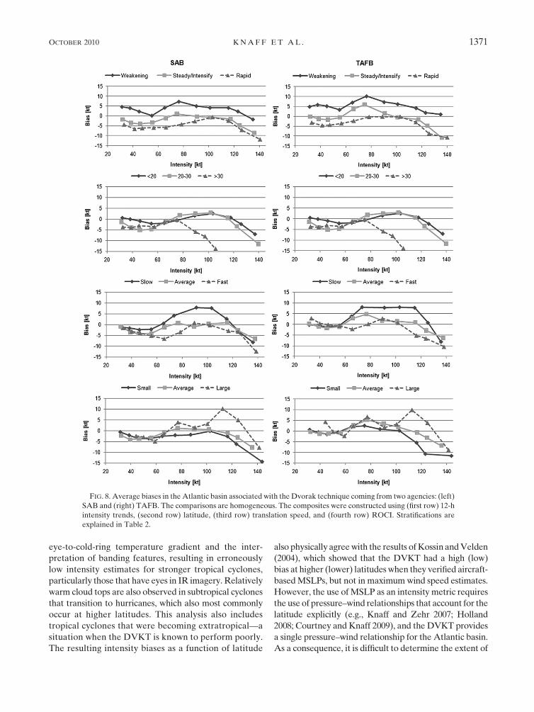
e. The effects of intensification, latitude, translation,and size
The same intensity binning methodology that is used
in section 4a is used here to further stratify the verification
results by 12-h intensification trends, latitude, translation
speed, and size or ROCI for the 1989–2008 Atlantic
samples. Each of the intensity bins is further subdivided
into three composites of each of these factors using the
ranges shown in Table 2. The data distributions de-
termined these ranges, which are approximately 61
standard deviation from the mean, except in the case of
ROCI, where the work of Kimball and Mulekar (2004)
was used as guidance. Results are shown in Fig. 8 and
the corresponding number of cases is listed in Table 3
for both agencies used in this study (TAFB and SAB).
These results show that the Dvorak intensity estimations
in general produce high and low biases for weakening and
strengthening, respectively. Upon closer examination,
this finding is primarily the result of biases associated
with DVKT intensity estimates for storms experienc-
ing the most rapid intensity changes, where weaken-
ing (strengthening) cases, produce pronounced large
high (low) biases. This finding suggests that the DVKT
intensification/weakening constraints [i.e., DVKT rules 8
(final T-number constraints) and 9 (CI number rules)]
may be too strict. The effects of translation speed also
show that fast- (slow-) moving storms have low (high)
biases associated with their intensity estimates. These
results support the discussions in Brown and Franklin
(2002, 2004), Holland (2008), Velden et al. (2006a), and
Courtney and Knaff (2009). These results suggest the
DVKT CI versus intensity table (Table 1) includes an
implicit climatological translation speed, which was not
documented in Dvorak (1972, 1975, 1984, or 1995).
The effects of variations of latitude seem primarily
confined to those storms poleward of 308 latitude and
with intensities greater than 80 kt. The probable cause
of these results is that the cloud-top temperatures used
with the EIR technique (Dvorak 1984) are warmer at
high latitudes. These warmer IR temperatures affect the
FIG. 7. The mean intensity difference between the first homo-
geneous pair of fixes from SAB and TAFB, plotted as a function of
the binned time difference between the first fix produced by each
agency. Note that the bins are large and the vast majority (199%)
of the fixes are separated by increments of 6 h 6 15 min.
TABLE 2. Description of the ranges of values used for the com-
posites of the DVKT intensity biases as a function of 12-h intensity
trend, latitude, translation speed, and ROCI.
12-h intensity trend (kt)
Weakening Steady/intensifying Rapid
,22.5 $22.5 and ,7.5 $7.5
Latitude (8N)
,20 $20 and ,30 $30
Translation speed (kt)
Slow Avg Fast
,6.0 $6.0 and ,14.0 $14.0
ROCI (n mi)
Small Avg Large
,165 $165 and ,270 $270
4 NHC changed its image analysis software from McIDAS to
NMAP, and the ATCF was updated to a UNIX version during
2000–02.
1370 W E A T H E R A N D F O R E C A S T I N G VOLUME 25
eye-to-cold-ring temperature gradient and the inter-
pretation of banding features, resulting in erroneously
low intensity estimates for stronger tropical cyclones,
particularly those that have eyes in IR imagery. Relatively
warm cloud tops are also observed in subtropical cyclones
that transition to hurricanes, which also most commonly
occur at higher latitudes. This analysis also includes
tropical cyclones that were becoming extratropical—a
situation when the DVKT is known to perform poorly.
The resulting intensity biases as a function of latitude
also physically agree with the results of Kossin and Velden
(2004), which showed that the DVKT had a high (low)
bias at higher (lower) latitudes when they verified aircraft-
based MSLPs, but not in maximum wind speed estimates.
However, the use of MSLP as an intensity metric requires
the use of pressure–wind relationships that account for the
latitude explicitly (e.g., Knaff and Zehr 2007; Holland
2008; Courtney and Knaff 2009), and the DVKT provides
a single pressure–wind relationship for the Atlantic basin.
As a consequence, it is difficult to determine the extent of
FIG. 8. Average biases in the Atlantic basin associated with the Dvorak technique coming from two agencies: (left)
SAB and (right) TAFB. The comparisons are homogeneous. The composites were constructed using (first row) 12-h
intensity trends, (second row) latitude, (third row) translation speed, and (fourth row) ROCI. Stratifications are
explained in Table 2.
OCTOBER 2010 K N A F F E T A L . 1371
the wind speed biases, if any, from the Kossin and Velden
(2004) study alone. The wind speed biases presented here
help clarify at what latitudes and intensities the intensity
biases are most pronounced in terms of wind speed. The
impacts of warmer cloud-top temperatures at higher lati-
tude result in DVKT intensity estimates that are too low, as
the most pronounced impacts on intensity estimation are at
latitudes greater than 30 8 and for storms with intensities
greater than 80 kt. We feel confident that this cloud-top
temperature effect is dominant, though it is worth
noting that latitude is correlated with 12-h intensity trends
(r 5 20.27) and ROCI (r 5 0.16), suggesting simply that
higher-latitude storms tend to be both larger and weak-
ening. These issues will be revisited in section 5.
The effects of tropical cyclone size on the DVKT in-
tensity estimates are also mostly confined to the higher-
intensity storms (those with intensities greater than
100 kt). Large storms are systematically overestimated
for intensities 100–125 kt and average and small storms
tend to be underestimated. This finding is believed to be
related to a combination of the application of the EIR
technique, scaling differences, and varying intensification
rates. In stronger TCs the extent of the coldest cloud is
related to tropical cyclone size and wind radii (Zehr and
Knaff 2007), suggesting a general proportionality among
the various TCs’ sizes. The relationship between the ra-
dial profiles of the IR brightness temperature and the
resulting TC wind field (i.e., proportionality) was further
demonstrated by the objective techniques developed by
Mueller et al. (2006) and Kossin et al. (2007), which
showed that the radial extent of the coldest cloud tops
was related to the radial extent of the winds and the
radius of maximum winds. IR imagery of small, average,
and large 125-kt cases with ROCI estimated at 100, 200,
and 300 n mi, respectively, visually shows this general
proportionality (Fig. 9). The EIR technique, which is
most commonly used because of its ability to make fixes
at all times, uses a specific one-size-fits-all width criteria
for the cold cloud ring that surround the eyewall (55 km
for 6.0 and 6.5 T numbers); ignoring the relative pro-
portionality among very strong storms. As a result, some
very small storms do not meet the minimum ring width
requirement necessary to reach the highest intensity
(i.e., CI) estimates. This was certainly the case for some
of the smallest storms examined in this study5 (e.g.,
Bret, 1145 UTC 22 August 1999; Felix, 1745 UTC
2 September 2007). However, it is more often the case
that the scaling shown in Fig. 9 effects both the mea-
surement of the eye temperature (too cold/not resolved)
and the ring width, as was the case with Hurricane
Charley (1745 UTC 13 August 2004).
The high bias associated with large tropical cyclones
in the intensity range 100–125 kt appears to be primarily
associated with the weakening phase of several cases. The
DVKT appears to not weaken several of these storms
fast enough and this is responsible for the high bias in
Fig. 8. Specific cases include Hurricane Floyd (1999)
during the period 1745 UTC 13 September–1745 UTC
14 September, Hurricane Katrina (2005) at 0615 and
1145 UTC 29 August, and Hurricane Rita (2005) during the
period 1745 UTC 22 September–2345 UTC 23 September.
This directly relates to DVKT rule 9 (CI rules), discussed
in Dvorak (1995) and in Velden et al. (1998), which limits
weakening, holding the T number constant from the peak
intensity during the first 12 h of weakening and then
holding the CI 0.5 to 1 T number higher as the storm
weakens. This result suggests that larger storms may
generally present cloud patterns that are suggestive of a
slower weakening and, when combined with the CI rules,
may result in an overestimation of this sample. However,
the sample is relatively small and this result is thus
tentative. It is also noteworthy that the large TC with
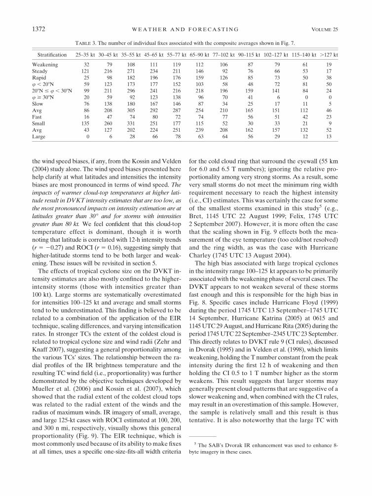
TABLE 3. The number of individual fixes associated with the composite averages shown in Fig. 7.
Stratification 25–35 kt 30–45 kt 35–55 kt 45–65 kt 55–77 kt 65–90 kt 77–102 kt 90–115 kt 102–127 kt 115–140 kt .127 kt
Weakening 32 79 108 111 119 112 106 87 79 61 19
Steady 121 216 271 234 211 146 92 76 66 53 17
Rapid 25 98 182 196 176 159 126 85 73 50 38
u , 208N 59 123 173 177 152 103 58 48 72 81 50
208N # u , 308N 99 211 296 241 216 218 196 159 141 84 24
u $ 308N 20 59 92 123 138 96 70 41 6 0 0
Slow 76 138 180 167 146 87 34 25 17 11 5
Avg 86 208 305 292 287 254 210 165 151 112 46
Fast 16 47 74 80 72 74 77 56 51 42 23
Small 135 260 331 251 177 115 52 30 33 21 9
Avg 43 127 202 224 251 239 208 162 157 132 52
Large 0 6 28 66 78 63 64 56 29 12 13
5 The SAB’s Dvorak IR enhancement was used to enhance 8-
byte imagery in these cases.
1372 W E A T H E R A N D F O R E C A S T I N G VOLUME 25

the largest high bias, mentioned above, also had eyewall
replacement cycles near peak intensity. The effects of
tropical cyclone size on DVKT intensity estimates, which
are seen at intensities greater than 100 kt, seem to be pri-
marily caused by changes in tropical cyclone scale with the
requirements for the largest DVKT intensities generally
being more difficult to obtain for the smaller storms. The
results of the large composite, which are dominated by
weakening cyclones in the 115–130-kt range further re-
iterates the likelihood that the CI rules for weakening are
too strict.
It is also noteworthy that, on average, all sizes of
tropical cyclones with intensities greater than 140 kt
(i.e., CI 5 7.0) are underestimated. To obtain a CI of
7.0, the storm must have a cold ring with a 55-km width
and a relatively warm eye. Closely examining the cases
used in this study, there are several causes for not meeting
these criteria. There are some cases when the eye was
unresolved by the ;4-km resolution of the geostationary
satellite imagery (e.g., Opal, 1145 UTC 4 October 1995;
Dennis, 1145 UTC 8 July 2005; Wilma, 2345 UTC
18 October 2005). Notably, Hugo (1989) at 1800 UTC
15 September also falls into this category due to the
steep viewing angle from GOES-7, but is not considered
in our dataset because of a lack of a ROCI estimate.
Some storms have eyewall replacement cycles that disrupt
the cold cloud tops and result in lower estimates (e.g.,
Isabel, 0615 UTC 13 September 2003; Ivan, 0645 UTC
13 September 2004). Other cases show that the cold cloud
tops are just not cold enough (e.g., Luis, 0645 UTC
4 September 1995; Isabel, 1745 UTC 14 September
2003; Felix, 2345 UTC 2 September 2007), which re-
iterates the potential effect of the relatively warm At-
lantic tropical tropopause temperature compared to the
Eastern Hemisphere during the months of November –
March (Newell and Gould-Stewart 1981; Seidel et al.
2001). There were also cases that had a combination
of too warm of a ring of cold cloud temperatures and
too cold eye temperatures in combination. So it appears
that, at least in this Atlantic sample, that there is a pro-
pensity for the EIR DVKT to underestimate very strong
FIG. 9. Examples of how tropical cyclones are scaled by size.
Shown are (top) Hurricane Iris (2001), (middle) Hurricane Dean
(2007), and (bottom) Hurricane Floyd (1999). Each storm has a best-
track intensity of 125 kt at the time of the image and ROCIs of 100,
200, and 300 n mi, respectively. Date and time information is pro-
vided for each panel, a 110-km circle is shown to provide spatial
scale, and the imagery is show on a sinusoidal equal area projection.
The temperature scale is provided at the bottom of the image.
OCTOBER 2010 K N A F F E T A L . 1373

tropical cyclones (.140 kt) because of 1) the relatively
warm climatological tropopause temperatures in the At-
lantic that make it difficult to observe cold rings with tem-
peratures colder than 2768C, 2) the occasional occurrence
of erroneous cold eye temperatures resulting from an in-
ability to resolve very small eyes and poor viewing an-
gles, and 3) the occasional disruption of the cold cloud
top and eye by eyewall replacement. The latter two points
are likely true in all tropical cyclone basins and were also
touched upon in Velden et al. (2006a), and the third point
suggests that the weakening of storms, in terms of wind
speed, during eyewall replacement cycles is less than
the DVKT would indicate. This last point is being ad-
dressed by adding microwave information to the ad-
vanced Dvorak technique (Olander and Velden 2007;
C. Velden 2010, personal communication).
Results using the 2002–08 Atlantic sample exhibited
similar patterns. However, the numbers of large cate-
gory 4 and 5 hurricanes are insufficient to address the
impacts of size on the biases.
5. Quantification and testing
a. Quantifying the various effects
Using the composites described in the previous sec-
tion, multiple linear regressions are used to quantify the
effects of each of these factors. The first step in this pro-
cess is to remove the biases that are solely a function of
intensity. This is accomplished by averaging the biases
from SAB and TAFB as a function of intensity, shown in
Fig. 3 (top), and then fitting a quadratic function to the
result as a function of best-track intensity (Vmax). Equa-
tion (1) below provides an estimate of the biases as a
function of Vmax. A similar procedure was performed that
quantifies the RMSE as a function of intensity and is
shown in (2). In application, one would use the estimated
Vmax to calculate the biases and RMSEs. Both equations
are valid for intensities ranging from 30 to 140 kt (or CI of
2.0 to 7.0). Above and below those values, users are ad-
vised to employ the estimates calculated at the closest
valid range:
Bias(Vmax
) 5 32.174� 1.990Vmax
1V
max
5.070
� �2
�V
max
15.076
� �3
1V
max
34.351
� �4
, (1)
RMSE(Vmax
) 5�10.887 1 0.748Vmax�
Vmax
11.196
� �2
1V
max
33.023
� �3
. (2)
To determine the effects of the various operational var-
iables composited in Fig. 8, the biases estimated from (1)
are then subtracted from the composites based on in-
tensity trend, latitude, translation speed, and ROCI. In
addition, a storm speed factor is introduced to better
parameterize for the effects of translation speed on the
tropical cyclone wind structure, particularly the maxi-
mum winds. The storm speed factor is equal to 1.5c0.63,
where c is the storm speed (in kt) to provide that portion
of the asymmetric wind field associated with translation;
these values (i.e., 1.5 and 0.63) ‘‘yielded satisfactory re-
sults’’ according to the developers Schwerdt et al. (1979).
Other applications (e.g., Demuth et al. 2006; Knaff and
Zehr 2007; Courtney and Knaff 2009) have also used this
formulation successfully for maximum wind applications.
The remaining residual biases are standardized (i.e., by
subtracting the mean and dividing by the standard de-
viation) and regressed against the mean standardized
values of intensity trend, storm speed factor, sine of lat-
itude (u), and ROCI that were created during the com-
positing procedures shown in Fig. 7. The means and
standard deviations of each variable along with the
normalized regression coefficients are shown in Table 4.
The resulting normalized regression coefficients show
that each of the factors is relatively important in de-
termining the resulting DVKT biases, with the intensity
trend having the greatest effect and the ROCI having
the least effect. Table 5 offers an estimate of the impacts
that each of these factors and their raw components have
on DVKT-based intensity estimation. These results also
appear to indirectly justify the use of the Schwerdt et al.
(1979) speed factor, which has a 20.86 kt21 sensitivity,
indirectly suggesting that it is a good approximation (i.e.,
close to 21.0 kt21 sensitivity). The sensitivities shown in
Table 5 are relatively small individually, given that in-
tensity is estimated to the nearest 5-kt interval, but in
combination they could produce larger biases.
Combining the results of (1) to the regression equa-
tion developed to estimate the impacts of the intensity
trend (DVmax), latitude (u), speed factor (i.e., 1.5c0.63),
and ROCI leads to a rather complicated equation for the
TABLE 4. List of factors associated with Dvorak intensity esti-
mation biases along with their mean and standard deviation values
for the Atlantic 1989–2008 sample. Also listed are the normalized
regression coefficients associated with each of these factors.
Factors Mean Std dev
Normalized regression
coefficients
Bias residual 20.049 3.356
Sin (latitude) 0.399 0.059 20.398
Speed factor (1.5c0.63) 6.316 1.211 20.310
ROCI (n mi) 196.753 43.227 0.211
Intensity trend 3.544 6.235 20.574
1374 W E A T H E R A N D F O R E C A S T I N G VOLUME 25

biases associated with the DVKT [see Eq. (3) below],
which explains 70% of the composite biases. In appli-
cation, DVmax would be estimated from the 12-h-old
operational intensity estimate and the current DVKT-
derived CI. Equation (3), as was the case for (1) and (2),
is valid for intensities ranging from 30 to 140 kt (or CI of
from 2.0 to 7.0). Above and below those values users are
advised to employ the estimates calculated at the closest
valid range. Equation (3) also was developed with few
cases equatorward of 128 latitude and poleward of 408
latitude (see Fig. 1), suggesting that those latitudes should
be used as a minimum and maximum value in application:
Bias 5 44.559� 1.990Vmax
1V
max
5.070
� �2
�V
max
15.076
� �3
1V
max
34.351
� �4
� 22.639 sin uj j� 0.859(1.5c0.63)
1 0.016ROCI� 0.309DVmax
. (3)
A similar procedure was performed for RMSE, but only
the intensity trend and latitude factors were statistically
significant, and the sensitivity of those factors was found
to be approximately two orders of magnitude less than
the effects of intensity alone. Thus, it appears that the
RMSE associated with the DVKT is primarily a function
of intensity, as shown in (2).
b. Testing bias corrections
Using the eastern North Pacific cases shown in Fig. 1,
the bias correction shown in (3) is tested. This is thought
to be a good test of (3) since the eastern Pacific sample
contains generally lower-latitude (16.58 versus 23.68),
slower-moving (8.1 versus 10.0 kt), and smaller tropical
cyclones (178 versus 197 n mi) when compared the At-
lantic basin. The 12-h intensity change of this sample is
2.0 kt versus the 3.5 kt found in the Atlantic sample.
From Tables 4 and 5, one might expect that the eastern
Pacific biases are high, and that is the case.
During 1989–2008, there were 49 cases when both
SAB and TAFB had DVTK intensity estimates within
62 h of aircraft reconnaissance. The intensities of this
sample range from 35 to 140 kt. SAB (TAFB) intensity
estimates had average biases of 4.53 kt (6.04 kt), MAEs
of 8.48 kt (8.74 kt), and RMSEs of 10.77 kt (11.34 kt)
before Eq. (3) is applied. Applying (3) to the individual
intensity estimates resulted in sample average SAB
(TAFB) biases of 2.12 kt (3.87 kt), MAEs of 7.19 kt
(7.80 kt), and RMSEs of 9.32 kt (9.89 kt). Since opera-
tional intensity estimates are reported to the nearest 5-kt
interval, intensity estimates from (3) were rounded to
the nearest 5-kt interval. This resulted in SAB (TAFB)
biases of 2.17 kt (4.14 kt), MAEs of 6.98 kt (7.66 kt),
and RMSEs of 9.48 kt (10.03 kt). These small changes
are nonetheless significant, resulting in 40%, 15%, and
11% reductions, respectively, in the intensity biases,
MAEs, and RMSEs of the total 98-case sample.
6. Summary, implications, and applications totropical cyclone analysis
The DVKT has been an important operational tool for
estimating tropical cyclone intensity and is the primary
basis for the global tropical cyclone intensity climatology
for the last 25 to 30 years. More recently, new satellite
techniques have been developed and are used in operations
to assess tropical cyclone intensities. However, the DVKT
remains the primary tool when aircraft reconnaissance is
unavailable for this exercise. The documentation provided
here gives the users of the raw DVKT intensity estimates
and the historical best tracks, based on the DVKT, quan-
titative estimates of the biases and errors associated with
this method based on a long and large Atlantic sample.
The findings of this study are based on DVTK practices
that have been used at SAB and TAFB. The practices at
SAB and TAFB closely follow those of Dvorak (1984).
Users of the DVKT in other basins have applied regional
variations and modifications to the DVKT (Velden et al.
2006b), which may have resulted in DVKT biases in those
regions that are different from those found in this study.
Given that caveat, this study has shown that the DVKT
has a tendency to slightly underestimate intensities of
storms receiving CI estimates ranging from 2.5 to 3.5
by an average of 1.5–2.5 kt, overestimate intensities of
storms receiving CI estimate ranging from 4.5 to 5.5 by
1.5–2.5 kt, and underestimate intensity estimates of storms
receiving CIs ranging from 6.5 to 7.0 by 4–9 kt. The DVKT
also has its best intensity estimate (signal) to RMSE
(noise) ratio in a range from 90 to 125 kt. Below 90 kt,
the technique has its least skill and above 125 kt the er-
rors increase. These situations suggest that the technique
has greater limitations when estimating maximum wind
speeds below 90 kt and above 125 kt. There is also an
indication that the DVKT may have difficulty discrimi-
nating between category 4 (114–135 kt) and category 5
TABLE 5. Estimates of Dvorak technique-based intensity bias
sensitivities examined by this study.
Factors Predicted bias sensitivity
Latitude (mean 5 23.58N) ’20.38 kt deg21
Sin latitude (mean 5 0.40) 222.6 kt (sin unit)21
Translation speed (mean 5 10.0 kt) ’20.55 kt kt21
Speed factor (mean 5 6.3 kt) 20.86 kt kt21
ROCI (mean 5 196 n mi) 0.016 kt (n mi)21
Intensity trend (mean 5 3.4) 20.31 kt kt21
OCTOBER 2010 K N A F F E T A L . 1375

(.135 kt) hurricanes in our Atlantic sample. This diffi-
culty appears to be related to cold cloud conditions
needed to obtain the highest DVKT intensities. Those
conditions are not as common as in the Eastern Hemi-
sphere during the months of November–March where the
climatological tropopause temperatures are colder. It is
worth noting that this result may not be applicable ev-
erywhere because, according to Harper (2002), the orig-
inal DVKT (i.e., Dvorak 1972, 1975) was developed using
a sample dominated by western North Pacific cases, and
that this is likely true of Dvorak (1984) as well. This study
also examined the first DVKT-based intensity estimate
coincident or prior to aircraft reconnaissance. The results
found using this limited sample show that the errors and
biases are similar to the larger Atlantic basin sample
where aircraft-based information could have influenced
the application of the DVKT. This should also provide
DVKT users some confidence that the influence and
availability of aircraft reconnaissance information does
not adversely affect the results of this study.
If the biases, which are a function of intensity (maxi-
mum wind speed), are accounted for, additional DVKT
biases are found to be related to 12-h intensity changes,
latitude, translational speed, and the ROCI. These re-
sults are generally consistent with past studies. Indi-
vidually, these factors result in relatively small biases
(Table 5), but the combination of these factors and the
built-in biases related solely to intensity can be appre-
ciable. Forecasters should be aware of these biases when
determining tropical cyclone intensities, be it operation-
ally or during any postevent reanalysis (i.e., ‘‘best track-
ing’’). Equation (3) provides a method for estimating the
biases of the DVKT based on these factors. Again, cau-
tion should be used in applying these results blindly to
other TC basins. There are several newly highlighted and
remaining shortcomings of the DVKT based on this At-
lantic sample. Translation speed, if faster or slower than
the sample mean, results in low or high biases, respec-
tively. The translation speed however can be accounted
for by using the Schwerdt et al. (1979) equation for
wind asymmetry. This speed factor has nearly a 1-to-1
correspondence with the biases related to the trans-
lation speed (i.e., Table 5). The average translation
speeds found for our sample were 7.5, 8.3, 8.7, 8.9, 9.1,
9.9, 11.0, 11.1, 11.2, 11.2, and 11.0 kt for CI numbers of
2.0, 2.5. . . 7.0, respectively. This finding highlights the
fact that weaker storms often move slower, which is
likely similar to the translation speeds that are implicit
in Table 1. It is clear that the rules associated with rapid
changes in intensity should be revisited and may be
abandoned given the frequency (typically half-hourly)
of the modern imagery, though this would require more
frequent intensity fixes. Currently, the DVKT rules do
not allow storms to intensify or weaken as fast as they
are observed to do so. The rule of holding storms at
peak intensity for 12 h and then keeping the CI from
1 to 0.5 T numbers higher during weakening, which has
been discussed by others (Brown and Franklin 2002;
Velden et al. 1998; Velden et al. 2006a), is also a rule
that should at the very least be accounted for when
assigning operational intensities. This rule, however,
should likely be formally reevaluated and eventually
modified for use in operations. This weakening issue is
an example of something that has already been ad-
dressed by regional modifications to the DVKT. High-
latitude DVKT intensity estimates are sometimes low
biased due to cold cloud-top temperatures being warmer
than in the deep tropics due to tropopause temperature
and height variations. This shortcoming is easily under-
stood and could likely be resolved by incorporating ad-
dition information either from global forecast model
analyses or from recent satellite imagery. With respect
to the size variations of intense cyclones (.95 kt), the
DVKT underestimates the intensity of the average and
small cyclones. Our results suggest that because different-
sized tropical cyclones scale to one another (Fig. 9), the
minimum requirements (cold cloud ring, eye tempera-
ture) used by the EIR DVKT for the higher intensities
are more difficult to obtain for smaller storms. The rela-
tively warm climatological tropopause temperatures in
the Atlantic, when compared to the western Pacific,
where most of the initial (i.e., Dvorak 1975) develop-
mental data were collected (Harper 2002), also seem to
be a factor in the DVKT’s relative inability to dis-
criminate strong category 4 from category 5 hurricanes
in this Atlantic sample. While it is likely that similar
biases are found in other TC basins, particularly those
biases related to the intensity, 12-h intensity change,
size (i.e., ROCI), and translation, caution should be used
when applying these results blindly to those TC basins,
particularly when regional modifications to the DVTK
practices have also been made.
It is notable that the digital Dvorak technique (Zehr
1989; Dvorak 1995), which has been carried over to the
objective Dvorak techniques described in Velden et al.
(1998) and Olander and Velden (2007), does not require
a minimum ring width and can be automated to estimate
an intensity and T number associated with every avail-
able image. The use of all available images and some
time averaging of the recent results may eventually en-
able the abandonment or at least the relaxation of the
DVKT CI rules. The advanced Dvorak technique (ADT;
Olander and Velden 2007), which already uses modified
pressure–wind relationships developed by Kossin and
Velden (2004) based on Atlantic aircraft data, also now
makes use of microwave image information that will
1376 W E A T H E R A N D F O R E C A S T I N G VOLUME 25

address center fix ambiguity as well as some of the in-
tensity estimation uncertainty between 35 kt, 2.5 T num-
ber, and 55 kt, 3.5 T number. Other intensity estimation
techniques, namely from the Advanced Microwave
Sounding Unit (AMSU; e.g., Herndon and Velden 2004;
Demuth et al. 2006), are being combined to form
consensus estimates that will further improve opera-
tional intensity estimates (C. Velden 2010, personal
communication).
The RMSEs associated with the DVKT are shown
here to be primarily a function of intensity [Fig. 3, Eq. (2)].
The DVKT appears to be designed to produce RMSEs
that are 0.5 T numbers when examined in terms of CI (i.e.,
given in Table 1). This result provides a measure of the
expected accuracy of the DVKT, and because the DVKT
is used as the primary intensity estimation tool at most
times and in most tropical cyclone basins, it offers an es-
timate of the errors associated with the historical best
tracks. Errors associated with the DVKT also can be
further reduced by using a consensus of DVKT fixes
from different agencies/analysts. Though a more com-
prehensive study is needed, this finding certainly suggests
that having multiple agencies providing independently
derived fixes to operations reduces the uncertainty as-
sociated with intensity estimation. Some coordination
between agencies, in particular, on policies (i.e., consis-
tent guidelines) as to when to consider initiating tropical
cyclone fixes, would result in more uniform DVKT re-
sults. Improving the initiation time of fixes would likely
result in more consistent, yet independent interagency
intensity fixes. Independence is important because it leads
to a better consensus estimate (Sampson et al. 2008, their
appendix B). These topics merit further investigation.
Also unresolved and deserving investigation is the po-
tential error reducing effects of more frequent DVKT
intensity estimation, which is now possible given the global
availability to more timely geostationary satellite imagery.
Biases and RMSEs associated with TAFB and SAB
DVKT estimates in the Atlantic basin during 1989–2008
have been quantified as a function of intensity in Eqs. (1)
and (2). Biases in this sample were also shown to be
a function of intensity, 12-h intensity trend, latitude,
translation speed, and size in terms of ROCI in Eq. (3).
Equation (3) has been applied to the eastern Pacific cases
with aircraft-influenced best-track intensity estimates in
those same 20 yr and has been shown to decrease the bias
by about 40% and the RMSE by about 10%. This makes
possible the creation of an intensity best track based
solely on the DVTK estimates and routinely available
operational information. The output would also contain
information about the expected RMSE. It is also note-
worthy that (1)–(3) are based on an Atlantic sample and
from fixes from TAFB and SAB and thus are likely most
applicable for DVKT estimates from those agencies and
in the Atlantic basin.
In the process of preparing this manuscript, it also
became clear that different agencies apply slightly dif-
ferent constraints to their fixes and use slightly different
procedures when arriving at their intensity estimates or
CIs. A discussion of regional modifications is included
in Velden et al. (2006b). This would suggest that the
RSMCs and other agencies, like SAB and JTWC, that
make intensity fixes could communicate more efficiently
and ultimately agree on one set of procedures to best
arrive at the DVKT CI. This would be a good exercise
for the World Meteorological Organization.
From a more practical standpoint, the information
provided here should 1) provide reassurance that the
DVKT is a skillful and internally consistent method that
has biases that are small compared to the RMSEs,
2) provide some of the known biases and expected ac-
curacies associated with making DVKT-based intensity
estimates based on an Atlantic sample, and 3) provide
some information as to where further studies are needed.
It is noteworthy that studies such as this one would not
be possible without the aircraft-based hurricane recon-
naissance available from the U.S. Air Force Reserve and
the National Oceanic and Atmospheric Administration
(NOAA) Aircraft Operations Center. This fact highlights
the desire for similar reconnaissance missions in other
tropical cyclone basins to better validate this and sim-
ilar studies. Despite the many caveats associated with
this study, we feel the results of this research will prove
useful for those in operational tropical cyclone forecast
centers, those performing climatological analyses with
the current best-track datasets, and those groups and
individuals conducting best-track reanalyses.
Acknowledgments. The authors thank Caroline Woods,
Mark Welshinger and Ken Barnett for helping locate
some of the historical literature; Ray Zehr, Chris Landsea,
Hugh Cobb, and Mark DeMaria for improving this paper
through an internal review process; and Chris Velden and
Andrew Burton who provided peer reviews. We also ac-
knowledge the countless individuals who left us won-
derful historical databases from which this study was
constructed. This research was supported by a NOAA
grant (NA17RJ1228). The views, opinions, and findings
contained in this report are those of the authors and
should not be construed as an official National Oceanic
and Atmospheric Administration or U.S. government
position, policy, or decision.
REFERENCES
Brown, D. P., and J. L. Franklin, 2002: Accuracy of pressure–wind
relationships and Dvorak satellite intensity estimates for
OCTOBER 2010 K N A F F E T A L . 1377

tropical cyclones determined from recent reconnaissance-based
‘‘best track’’ data. Preprints, 25th Conf. on Hurricanes and Trop-
ical Meteorology, San Diego, CA, Amer. Meteor. Soc., 458–459.
——, and ——, 2004: Dvorak TC wind speed biases determined
from reconnaissance-based best track data (1997–2003). Pre-
prints, 26th Conf. on Hurricanes and Tropical Meteorology,
Miami, FL, Amer. Meteor. Soc., 86–87.
Burton, A. D., 2005: Notes on the application of the Dvorak
technique. Bureau of Meteorology Meteorological Note 225,
8 pp.
Courtney, J., and J. A. Knaff, 2009: Adapting the Knaff and Zehr
pressure–wind relationship for operational use in Tropical Cy-
clone Warning Centres. Aust. Meteor. Oceanogr. J., 58, 167–179.
Demuth, J., M. DeMaria, and J. A. Knaff, 2006: Improvement of
Advanced Microwave Sounder Unit tropical cyclone intensity
and size estimation algorithms. J. Appl. Meteor. Climatol., 45,
1573–1581.
Dvorak, V. F., 1972: A technique for the analysis and forecasting of
tropical cyclone intensities from satellite pictures. NOAA Tech.
Memo. NESS 36, 15 pp. [Available from NOAA/NESDIS,
5200 Auth Rd., Washington, DC 20333.]
——, 1975: Tropical cyclone intensity analysis and forecasting from
satellite imagery. Mon. Wea. Rev., 103, 420–430.
——, 1984: Tropical cyclone intensity analysis using satellite data.
NOAA Tech. Rep. 11, 45 pp. [Available from NOAA/NESDIS,
5200 Auth Rd., Washington, DC 20333.]
——, 1995: Tropical clouds and cloud systems observed in satellite
imagery: Tropical cyclones. Workbook Vol. 2. NOAA/NESDIS,
359 pp. [Available from NOAA/NESDIS, 5200 Auth Rd.,
Washington, DC 20333.]
Franklin, J. L., M. L. Black, and K. Valde, 2003: GPS dropwind-
sonde wind profiles in hurricanes and their operational im-
plications. Wea. Forecasting, 18, 32–44.
Gaby, D., J. Lushine, B. Mayfield, S. Pearce, and F. Torres, 1980:
Satellite classifications of Atlantic tropical and subtropical
cyclones: A review of eight years of classifications at Miami.
Mon. Wea. Rev., 108, 587–595.
Guard, C. P., 1988: Tropical cyclone studies: Part 3—Results of
a tropical cyclone accuracy study using polar orbiting satellite
data. FCM-R11-1988, Federal Coordinator for Meteorologi-
cal Services and Supporting Research, 3-1–3-36. [Available
from Office of the Federal Coordinator for Meteorology, 8455
Colesville Rd., Ste. 1500, Silver Spring, MD 20910.]
Harper, B. A., 2002: Tropical cyclone parameter estimation in the
Australian region—Wind–pressure relationships and related
issues for engineering planning and design—A discussion pa-
per. SEA Rep. J0106-PR003E, Systems Engineering Australia
Pty. Ltd. (SEA) for Woodside Energy, Ltd., 83 pp. [Available
from Systems Engineering Australia Pty. Ltd., 106/71 Beeston
St., Newstead, QLD, 4006, Australia.]
——, S. A. Stroud, M. McCormack, and S. West, 2008: A review of
historical tropical cyclone intensity in northwestern Australia
and implications for climate change trend analysis. Aust. Me-
teor. Mag., 57, 121–141.
Herndon, D., and C. Velden, 2004: Upgrades to the UW-CIMSS
AMSU-based TC intensity algorithm. Preprints, 26th Conf. on
Hurricanes and Tropical Meteorology, Miami, FL, Amer.
Meteor. Soc., 118–119.
Holland, G., 2008: A revised hurricane pressure–wind model. Mon.
Wea. Rev., 136, 3432–3445.
Kimball, S. K., and M. S. Mulekar, 2004: A 15-year climatology of
North Atlantic tropical cyclones. Part I: Size parameters.
J. Climate, 17, 3555–3575.
Knaff, J. A., and R. M. Zehr, 2007: Reexamination of tropical cy-
clone wind–pressure relationships. Wea. Forecasting, 22, 71–88.
——, and ——, 2008: Reply. Wea. Forecasting, 23, 762–770.
Koba, H., S. Osano, T. Hagiwara, S. Akashi, and T. Kikuchi, 1990:
Relationship between the CI-number and central pressure and
maximum wind speed in typhoons (in Japanese). J. Meteor.
Res., 42, 59–67.
——, ——, ——, ——, and ——, 1991: Relationship between the
CI-number and central pressure and maximum wind speed in
typhoons (English translation). Geophys. Mag., 44, 15–25.
Kossin, J. P., and C. S. Velden, 2004: A pronounced bias in tropical
cyclone minimum sea level pressure estimation based on the
Dvorak technique. Mon. Wea. Rev., 132, 165–173.
——, J. A. Knaff, H. I. Berger, D. C. Herndon, T. A. Cram,
C. S. Velden, R. J. Murnane, and J. D. Hawkins, 2007: Esti-
mating hurricane wind structure in the absence of aircraft
reconnaissance. Wea. Forecasting, 22, 89–101.
Mayfield, M., C. J. McAdie, and A. C. Pike, 1988: Tropical cyclone
studies. Part 2—A preliminary evaluation of the dispersion of
tropical cyclone position and intensity estimates determined
from satellite imagery. FCM-R11-1988, Federal Coordinator for
Meteorological Services and Supporting Research, 2-1–2-17.
[Available from Office of the Federal Coordinator for Meteo-
rology, 8455 Colesville Rd., Ste. 1500, Silver Spring, MD 20910.]
Mueller, K. J., M. DeMaria, J. A. Knaff, J. P. Kossin, and
T. H. Vonder Haar, 2006: Objective estimation of tropical
cyclone wind structure from infrared satellite data. Wea.
Forecasting, 21, 990–1005.
Nakazawa, T., and S. Hoshino, 2009: Intercomparison of Dvorak
parameters in the tropical cyclone datasets over the western
North Pacific. Sci. Online Lett. Atmos., 5, 33–36, doi:10.2151/
sola.2009-009.
Newell, R. E., and S. Gould-Stewart, 1981: A stratospheric foun-
tain? J. Atmos. Sci., 38, 2789–2796.
Olander, T. L., and C. S. Velden, 2007: The advanced Dvorak
technique: Continued development of an objective scheme to
estimate tropical cyclone intensity using geostationary in-
frared satellite imagery. Wea. Forecasting, 22, 287–298.
Peterson, T. C., and Coauthors, 1998: Homogeneity adjustments of
in situ atmospheric climate data: A review. Int. J. Climatol., 18,
1493–1517.
Sampson, C. R., and A. J. Schrader, 2000: The Automated Tropical
Cyclone Forecasting system (version 3.2). Bull. Amer. Meteor.
Soc., 81, 1231–1240.
——, J. L. Franklin, J. A. Knaff, and M. DeMaria, 2008: Experi-
ments with a simple tropical cyclone intensity consensus. Wea.
Forecasting, 23, 304–312.
Schwerdt, R. W., F. P. Ho, and R. R. Watkins, 1979: Meteorological
criteria for standard project hurricane and probable maximum
hurricane wind fields, Gulf and East Coasts of the United
States. NOAA Tech. Rep. NWS 23, 317 pp. [Available from
National Hurricane Center Library, 11691 SW 117 St., Miami
FL 33165-2149.]
Seidel, D. J., R. J. Ross, J. K. Angell, and G. C. Reid, 2001: Cli-
matological characteristics of the tropical tropopause as re-
vealed by radiosondes. J. Geophys. Res., 106, 7857–7878.
Sheets, R. C., and C. McAdie, 1988: Tropical cyclone studies. Part
1—Preliminary results of a study of the accuracy of satellite-
based tropical cyclone position and intensity estimates. FCM-
R11-1988, Federal Coordinator for Meteorological Services
and Supporting Research, 1-1–1-49. [Available from Office of
the Federal Coordinator for Meteorology, 8455 Colesville
Rd., Ste. 1500, Silver Spring, MD 20910.]
1378 W E A T H E R A N D F O R E C A S T I N G VOLUME 25
Velden, C. S., T. Olander, and R. M. Zehr, 1998: Development of
an objective scheme to estimate tropical cyclone intensity
from digital geostationary satellite imagery. Wea. Forecasting,
13, 172–186.
——, and Coauthors, 2006a: The Dvorak tropical cyclone in-
tensity estimation technique: A satellite-based method that
has endured for over 30 years. Bull. Amer. Meteor. Soc., 87,
1195–1210.
——, and Coauthors, 2006b: Supplement to: The Dvorak tropical
cyclone intensity estimation technique: A satellite-based
method that has endured for over 30 years. Bull. Amer. Meteor.
Soc., 87 (Suppl.), S6–S9, doi:10.1175/BAMS-87-9-Velden.
WMO, 2000: Twenty years of progress and achievement of the WMO
Tropical Cyclone Programme (1980-1999). WMO/TD-1039,
Rep. TCP-43, World Meteorological Organization, Geneva,
Switzerland, 36 pp.
Zehr, R. M., 1989: Improved objective satellite estimates of trop-
ical cyclone intensity. Preprints, 18th Conf. on Hurricanes and
Tropical Meteorology, San Diego, CA, Amer. Meteor. Soc.,
J25–J28.
——, and J. A. Knaff, 2007: Atlantic major hurricanes, 1995–
2005—Characteristics based on best track, aircraft, and IR
images. J. Climate, 20, 5865–5888.
——, J. L. Beven II, and M. DeMaria, cited 2010: Analysis of high
resolution infrared images of hurricanes from polar satellites
as a proxy for GOES-R. [Available online at http://www.
goes-r.gov/downloads/GOES%20Users’%20Conference%
20IV/Complete%20Posters/GUC4_poster_Zehr.ppt.]
OCTOBER 2010 K N A F F E T A L . 1379