Please cite this document as:

A. B. Lambe, J. R. R. A. Martins, and G. J. Kennedy. An evaluation of constraint aggregation strategies for wing boxmass minimization. Structural and Multidisciplinary Optimization, 55(1):257–277, January 2017.This document can be found at: http://mdolab.engin.umich.edu.

An Evaluation of Constraint Aggregation Strategies forWing Box Mass Minimization

Andrew B. Lambe1, Graeme J. Kennedy2, Joaquim R. R. A. Martins3

Abstract Constraint aggregation makes it feasible to solve large-scale stress-constrained mass mini-mization problems efficiently using gradient-based optimization where the gradients are computed usingadjoint methods. However, it is not always clear which constraint aggregation method is more effective, andwhich values to use for the aggregation parameters. In this work, the accuracy and efficiency of several ag-gregation methods are compared for an aircraft wing design problem. The effect of the type of aggregationfunction, the number of constraints, and the value of the aggregation parameter are studied. Recommen-dations are provided for selecting a constraint aggregation scheme that balances computational effort withthe accuracy of the computed optimal design. Using the recommended aggregation method and associatedparameters, a mass of within 0.5% of the true optimal design was obtained.

1 IntroductionWe are interested in the problem of minimizing structural mass subject to constraints on structural failure. Inparticular, we are interested in failure criteria based on yield stress and buckling under static loads. Checkingthe failure criteria in the optimization problem is desirable from an engineering design perspective becausedoing so allows us to immediately verify that the structure is suitable for the prescribed loading conditions.

The primary issue with including failure constraints directly in the structural optimization problem is theresulting size of the optimization problem. Conceptually, for a continuum structure, failure constraints needto be enforced throughout the material domain, leading to an infinite number of constraints. More practically,failure constraints may be enforced element-wise in the finite element model. For detailed, high-fidelitystructural models, this can lead to an optimization problem with many thousands or millions of failureconstraints. These constraints are costly to enforce because they can only be checked by completing thestructural analysis. Specialized algorithm implementations are required to solve the optimization problemefficiently (Duysinx and Bendsøe, 1998).

The number of constraints in the optimization problem can be reduced through aggregation. The con-straint aggregate then represents an effective failure criteria evaluated over a large part of the material do-main. A natural choice for these constraint aggregates is a maximum- or minimum-value function. How-ever, the maximum- and minimum-value functions are not differentiable and cannot be used efficiently inconjunction with gradient-based design optimization. Instead, these functions are replaced by smooth es-timators like the Kreisselmeier–Steinhauser (KS) function (Kreisselmeier and Steinhauser, 1979, 1983) orthe p-norm function (Duysinx and Sigmund, 1998; Qiu and Li, 2010). These estimators do not preciselyreproduce the true feasible design space provided by the original constraints, so the final design determinedby the optimizer will be different depending on the aggregation scheme.

1Postdoctoral Fellow, Department of Mechanical Engineering, York University, Toronto, Ontario, Canada2Assistant Professor, School of Aerospace Engineering, Georgia Institute of Technology, Atlanta, Georgia, USA3Professor, Department of Aerospace Engineering, University of Michigan, Ann Arbor, Michigan, USA

1

Because of the need to aggregate failure constraints, there exists a natural compromise between the qual-ity of the optimal structural design, i.e., how close the computed design is to the “true” optimal solution thatcould be computed by the model, and the computational effort to find it. This compromise has been observedin the literature before, particularly in the field of topology optimization. Parıs et al. (2009, 2010) comparedthe use of local stress constraints with a global stress constraint (aggregation into one failure constraint)and block aggregation of contiguous regions of the structure. Their results confirm our intuition about thetrade-off: local constraints produce the highest quality results, but block aggregation greatly reduces thecomputational expense. However, their results only compare a single choice for the number of blocks, oraggregation domains, with global aggregation and no aggregation. No information is given about how tochoose the number of aggregation domains.

Le et al. (2010) compared aggregation based on physical location in the design domain with aggrega-tion based on the stress distribution. In the latter scheme, an interlacing approach was used in which theelements were sorted based on the failure criteria and every m elements in order were allocated to m differ-ent constraints. While this scheme gives better control over local constraint violation, (the highly stressedelements are aggregated to many different constraints, reducing aggregation error,) it results in changes tothe optimization problem formulation every time the elements are sorted and reallocated. Consequently, thischanging problem statement may impede the convergence of the optimizer. Holmberg et al. (2013) study a“stress level” aggregation scheme in which elements with similar stresses are grouped in the same failureconstraint. They also consider cases in which the elements are reallocated infrequently, rather than at eachiteration. However, only the effects on the final solution are examined in detail in this study.

What is missing from the previous research is a detailed study of the influence of the aggregation schemeon computational effort. In this paper, we take aggregation scheme to mean both the number of constraints,the choice of aggregation function, and the choice of parameters in the aggregation function. In all cases,we take the aggregation domains to be fixed and based on physical location. While not as advanced as someof the other methods mentioned above, this approach is easy to implement, requires no a priori knowledgeabout the problem, and will not alter the problem formulation as the optimization algorithm progresses. Weaim to provide general recommendations for solving failure constrained mass minimization problems usingaggregation to balance low computational effort with accuracy of the optimal solution.

Another important contribution of this work is a comparative study of classical and induced aggregationmethods. Induced aggregation methods were recently introduced by Kennedy and Hicken (2015) with theaim of providing greater accuracy in the optimal solution under aggregated constraints. This paper representsthe first detailed comparison of these two classes of aggregate.

Our application of interest is aircraft wing design. Our previous studies of both structural and mul-tidisciplinary (aerostructural) wing design subject to failure constraints (Kenway et al., 2014b; Kennedyand Martins, 2014b; Kenway and Martins, 2014; Kenway et al., 2014a) generally used a small number ofKS aggregation functions with a fixed choice of parameter. We have also experimented with specializedoptimizers which can accommodate a large number of design constraints (Lambe and Martins, 2015) andoptimizers that tightly integrate adaptive constraint aggregation (Kennedy, 2015). In this paper, we use awing design problem to examine the effects of varying the aggregation scheme. Our problem contains bothmaterial yield constraints and buckling constraints.

The remainder of this paper is organized as follows. Section 2 reviews the major approaches to con-straint aggregation in the literature. Section 3 lays out our wing design test problem and our analysis andoptimization software. Section 4 discusses the optimization results of the different aggregation schemes.Section 5 makes recommendations for applying constraint aggregation to general mass minimization prob-lems. Finally, Section 6 summarizes our work.

2

2 Review of Constraint Aggregation TechniquesIn this paper, we are concerned with minimizing structural mass subject to a bound on a measure of the localstress. We write the local stress or failure constraint as

g(ξ ,~x,~u)≤ 1,

where ξ ∈ Ω is a point within the structural domain Ω, ~x are the design variables, and ~u are the structuraldegrees of freedom. Common failure constraints include the von Mises yield criterion which can be writtenas

g =σv

σd,

where σv is the von Mises stress and σd is the design stress. Throughout the following, we omit the argu-ments to the failure function g to simplify our notation.

As previously described, one method to impose the bound g≤ 1 everywhere within the structural domainis to use the maximum-value function such that

maxξ∈Ω

g = maxg≤ 1. (1)

However, because the constraint (1) is not smooth, efficient gradient-based optimization algorithms cannotbe used to solve the resulting optimization problem. Instead, we use smooth constraint aggregation functions~c ∈ RM to approximately impose maxg ≤ 1 over M disjoint partitions of the structural domain Ωk, k =1, . . . ,M. These functions satisfy the limit property

limρ→∞

~ck(g,ρ) = maxξ∈Ωk

g k = 1, . . . ,M. (2)

Increasing the parameter ρ simultaneously reduces the aggregation error while also making the optimizationproblem more difficult to solve with a gradient-based optimizer due to the increased curvature in regionswhere the maximum-value function is not differentiable. Therefore, we are interested in selecting functionsfor which moderate values of ρ yield accurate constraint aggregates.

To review the different constraint aggregation approaches, we make reference to the following modelproblem.

minimize m(~x)

with respect to ~x,~u

such that ~c(g,ρ)≤ 1

governed by ~K(~x)~u = ~f .

(3)

In this problem, m(~x) represents the structural mass, and ~K(~x)~u = ~f represents the finite element governingequations.

We solve the optimization problem (3) using two types of constraint aggregates: discrete and continuous.Discrete aggregates operate on a finite set of stress constraints that are obtained by evaluating g at trialpoints within the structural domain. Typically, these trial points correspond to the quadrature points in eachelement. As a result of this construction, some discrete aggregates exhibit mesh-dependence (Kennedy andHicken, 2015). In contrast, continuous aggregation techniques seek an approximation of the maximum valuefunction using integrals over the domain. As a result, continuous aggregates have a well-defined limit forincreasing mesh size. However, for a fixed mesh the discrete and continuous aggregates share the samelimit as ρ increases if the quadrature scheme for the continuous aggregate shares the same trial points as thediscrete aggregate.

3

One elusive property of constraint aggregation methods is conservatism. An aggregate c is said to beconservative if, given a threshold parameter value ρ∗,

c(g,ρ)> maxg ∀ρ > ρ∗. (4)

In other words, the estimate of the maximum value produced by a conservative aggregate is necessarilyan overestimate. As a result, a conservative aggregate would guarantee g ≤ 1 everywhere within the do-main. Unfortunately, to our knowledge, a truly conservative aggregate does not exist for an arbitrary stressdistribution, g. While some discrete aggregates, such as the KS function and p-norm, are discretely con-servative, they make no guarantees about the value of the stress constraint at points other than the triallocations (Kennedy and Hicken, 2015).

2.1 Classical Constraint Aggregation

In this section, we review two classical approaches to constraint aggregation: Kreisselmeier–Steinhauser(KS) aggregation (Kreisselmeier and Steinhauser, 1979, 1983; Akgun et al., 2001) and p-norm aggrega-tion (Duysinx and Sigmund, 1998; Qiu and Li, 2010). When applied to the continuous constraint g, theseaggregation approaches reduce to functionals over the domain Ω. The KS functional is given by

cKS(g,ρ) =1ρ

ln[

1α

∫Ω

eρgdΩ

]= k+

1ρ

ln[

1α

∫Ω

eρ(g−k)dΩ

],

(5)

where α > 0 is a normalization factor and k is an arbitrary constant. The factor α is typically chosen tobe either 1 or |Ω|, but may be chosen arbitrarily provided it does not affect the asymptotic convergence ofthe functional at large values of ρ (Kennedy and Hicken, 2015). The second form of the KS functional ispreferable when using finite-precision arithmetic since very large powers of e can be avoided with a suitablechoice of k. The p-norm functional is given by

cPN(g,ρ) =[

1α

∫Ω

|g|ρdΩ

] 1ρ

= k[

1α

∫Ω

∣∣∣gk

∣∣∣ρ dΩ

] 1ρ

(6)

where α > 0 and k > 0 have the same meaning as in the KS functional. Again, the second form of thefunctional is preferable when finite-precision arithmetic is used. Despite calling Equation (6) a p-normfunctional, we use ρ as the norm value for consistency in the presentation of the different methods.

The presence of the absolute value operator in the p-norm functional compromises its applicability asan aggregator. If g can take both positive and negative values, then the functional is not differentiable inregions where g transitions from positive to negative. For some failure criteria, such as the von Mises stresscriterion, this is not an issue because g is restricted to nonnegative real values. If the failure criterion hasa finite, negative lower bound, such as the Tsai–Wu failure criterion, the criterion should be remapped tononnegative real values to exploit p-norm aggregation. If g can take arbitrarily negative values, for instancein buckling envelope calculations, remapping is not possible and the KS functional is recommended instead.

Both the KS and p-norm functionals have analogues for finite sets of constraints. Let us define a finiteset of constraints by selecting nt trial points in Ω at which to check for failure. Let ξi, i = 1, ...,nt be the trialpoint locations and gi = g(ξi,~x,~u) be the constraint values at the trial points. The KS function for this set of

4

constraints is

cDKS(ρ) =1ρ

ln

[nt

∑i=1

eρgi

]

= maxi

gi +1ρ

ln

[nt

∑i=1

eρ(gi−maxi gi)

],

(7)

while the p-norm function is

cDPN(ρ) =

[nt

∑i=1|gi|ρ

] 1ρ

= maxi|gi|

[nt

∑i=1

∣∣∣∣ gi

maxi gi

∣∣∣∣ρ] 1

ρ

.

(8)

On the right side of both Equations (7) and (8), we have chosen the constant k to be the maximum value ofg obtained in the trial points.

2.2 Induced Constraint Aggregation

Recently, Kennedy and Hicken (2015) introduced a new class of aggregation methods known as inducedaggregation methods. Induced aggregates are designed to provide more accurate estimates of maxg for agiven value of ρ than classical aggregates. We focus on two aggregation functionals within the class ofinduced aggregates which are closely related to the KS and p-norm functionals. The induced exponentialfunctional is given by

cIE(g,ρ) =∫

ΩgeρgdΩ∫

ΩeρgdΩ

. (9)

Kennedy and Hicken (2015) show how cIE can be obtained from cKS by taking a Richardson extrapolationof cKS to ρ → ∞. The induced power functional is given by

cIP(g,ρ) =∫

Ωgρ+1dΩ∫

ΩgρdΩ

. (10)

The induced power functional is only suited to strictly positive functions g (Kennedy and Hicken, 2015).This is analogous to the p-norm functional requiring nonnegative g values to be effective.

The induced aggregation functionals also have discrete analogues for finite sets of constraints. Theinduced exponential function is given by

cDIE(ρ) =∑

nti=1 gieρgi

∑nti=1 eρgi

. (11)

The induced power function is given by

cDIP(ρ) =∑

nti=1 gρ+1

i

∑nti=1 gρ

i. (12)

Similar to cIP, cDIP is only applicable if gi ≥ 0 for i = 1, ...,nt . One advantage these induced aggregationfunctions possess over the classical aggregation functions is convergence to a single value for an arbitrarynumber of sample points. This is evident from the fact that functions (11) and (12) are ratios of sums ratherthan single sums.

5

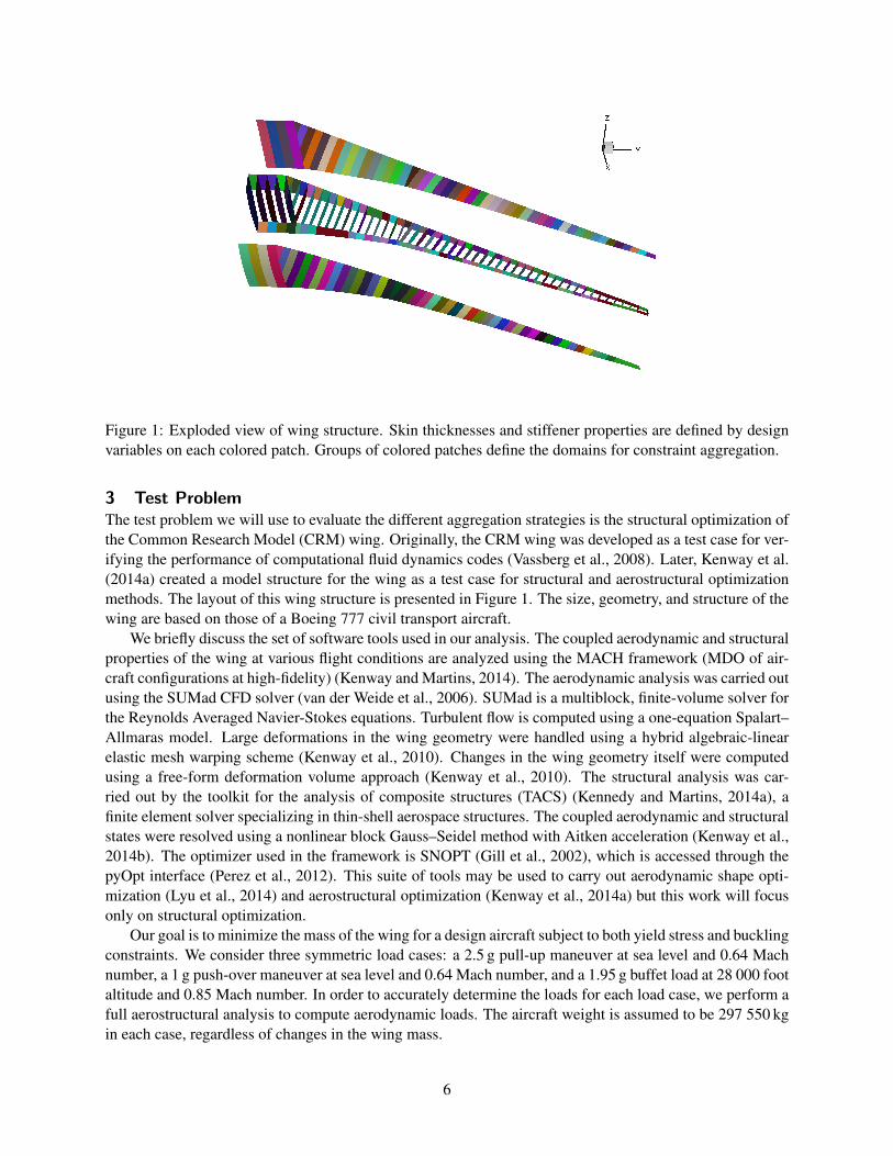
Figure 1: Exploded view of wing structure. Skin thicknesses and stiffener properties are defined by designvariables on each colored patch. Groups of colored patches define the domains for constraint aggregation.

3 Test ProblemThe test problem we will use to evaluate the different aggregation strategies is the structural optimization ofthe Common Research Model (CRM) wing. Originally, the CRM wing was developed as a test case for ver-ifying the performance of computational fluid dynamics codes (Vassberg et al., 2008). Later, Kenway et al.(2014a) created a model structure for the wing as a test case for structural and aerostructural optimizationmethods. The layout of this wing structure is presented in Figure 1. The size, geometry, and structure of thewing are based on those of a Boeing 777 civil transport aircraft.

We briefly discuss the set of software tools used in our analysis. The coupled aerodynamic and structuralproperties of the wing at various flight conditions are analyzed using the MACH framework (MDO of air-craft configurations at high-fidelity) (Kenway and Martins, 2014). The aerodynamic analysis was carried outusing the SUMad CFD solver (van der Weide et al., 2006). SUMad is a multiblock, finite-volume solver forthe Reynolds Averaged Navier-Stokes equations. Turbulent flow is computed using a one-equation Spalart–Allmaras model. Large deformations in the wing geometry were handled using a hybrid algebraic-linearelastic mesh warping scheme (Kenway et al., 2010). Changes in the wing geometry itself were computedusing a free-form deformation volume approach (Kenway et al., 2010). The structural analysis was car-ried out by the toolkit for the analysis of composite structures (TACS) (Kennedy and Martins, 2014a), afinite element solver specializing in thin-shell aerospace structures. The coupled aerodynamic and structuralstates were resolved using a nonlinear block Gauss–Seidel method with Aitken acceleration (Kenway et al.,2014b). The optimizer used in the framework is SNOPT (Gill et al., 2002), which is accessed through thepyOpt interface (Perez et al., 2012). This suite of tools may be used to carry out aerodynamic shape opti-mization (Lyu et al., 2014) and aerostructural optimization (Kenway et al., 2014a) but this work will focusonly on structural optimization.

Our goal is to minimize the mass of the wing for a design aircraft subject to both yield stress and bucklingconstraints. We consider three symmetric load cases: a 2.5 g pull-up maneuver at sea level and 0.64 Machnumber, a 1 g push-over maneuver at sea level and 0.64 Mach number, and a 1.95 g buffet load at 28 000 footaltitude and 0.85 Mach number. In order to accurately determine the loads for each load case, we perform afull aerostructural analysis to compute aerodynamic loads. The aircraft weight is assumed to be 297 550 kgin each case, regardless of changes in the wing mass.

6

b

wb

hs

tstb

tw

Figure 2: Cross-section of a skin panel with the design parameters labelled. Only skin thickness ts, stiffenerheight hs, stiffener thickness tw, and stiffener pitch b are independent variables in our problem.

The design variables of the problem are the thicknesses of the skin panels ts, the stiffener height hs, thestiffener thickness tw, and the distance between stiffeners b, known as the pitch. The colored patches shownin Figure 1 represent stiffened skin panels over which individual design variables apply. Figure 2 showsa cross-section of a typical skin panel and the definition of each variable. For simplicity, we let tb = twand wb = hs in the stiffener model. In addition, a single variable defines the stiffener pitch on the entirelower skin, the entire upper skin, and both wing spars. Linear adjacency constraints are introduced for thethickness, stiffener thickness, and stiffener height variables to restrict the difference between the variablevalues in adjacent skin panels. In our finite element model, instead of modeling the stiffeners directly, theincrease in stiffness resulting from the stiffeners is smeared over the whole panel. In total, the problemcontains 842 design variables and 660 linear constraints.

The failure criteria of the problem are aggregated over the four main wing components: lower skin,upper skin, spars, and ribs. Each component has one yield stress failure criterion and one buckling failurecriterion per load case, for a total of 24 constraints. This number is reduced to 17 failure constraints byignoring buckling for the wing skin that is in tension in each load case and ignoring yield stress failure forthe 1.95 g buffet load case. The latter simplification is justified because those constraints are supersededby the yield stress failure in the 2.5 g load case. The number of constraints is altered by subdividing eachcomponent into more aggregation domains. We use between one and 40 domains per component, yieldingbetween 17 and 680 failure constraints in the optimization problem.

4 Aggregation Strategy ComparisonIn Section 2, we defined eight different functions that could be used for aggregating failure constraints in astructural optimization problem. In addition to selecting the aggregation function, the user must also selectthe aggregation parameter ρ and the number of domains into which the structure is split. As stated in theintroduction, choosing larger parameter values and splitting the structure into more aggregation domainsleads to a more accurate optimal mass estimate, but increases the cost of the optimization. Our goal with theremainder of this paper is to quantify the trade-off between accuracy and computational cost as we vary theaggregation scheme.

As stated in the Section 1, each aggregation scheme comprises a choice of aggregation function, achoice of aggregation parameter ρ , and a choice of how many domains into which each wing componentis divided. Each component may be divided into one, two, five, ten, 20, or 40 smaller domains. For eachchoice of domains, we choose from among 13 possible values of aggregation parameter between 20 and 500and one of the eight aggregation functions described earlier. This yields a total of 624 possible aggregation

7

0.00 0.01 0.02 0.03 0.04 0.05 0.061/ρ

14000

14500

15000

15500

16000

16500

Optimal Mass(kg)

1 DKS2 DKS5 DKS

10 DKS20 DKS40 DKS

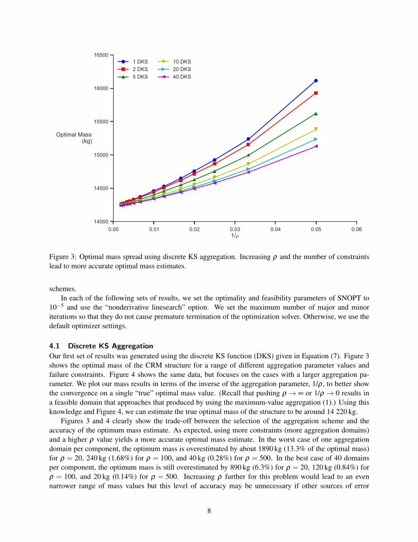
Figure 3: Optimal mass spread using discrete KS aggregation. Increasing ρ and the number of constraintslead to more accurate optimal mass estimates.

schemes.In each of the following sets of results, we set the optimality and feasibility parameters of SNOPT to

10−5 and use the “nonderivative linesearch” option. We set the maximum number of major and minoriterations so that they do not cause premature termination of the optimization solver. Otherwise, we use thedefault optimizer settings.

4.1 Discrete KS Aggregation

Our first set of results was generated using the discrete KS function (DKS) given in Equation (7). Figure 3shows the optimal mass of the CRM structure for a range of different aggregation parameter values andfailure constraints. Figure 4 shows the same data, but focuses on the cases with a larger aggregation pa-rameter. We plot our mass results in terms of the inverse of the aggregation parameter, 1/ρ , to better showthe convergence on a single “true” optimal mass value. (Recall that pushing ρ → ∞ or 1/ρ → 0 results ina feasible domain that approaches that produced by using the maximum-value aggregation (1).) Using thisknowledge and Figure 4, we can estimate the true optimal mass of the structure to be around 14 220 kg.

Figures 3 and 4 clearly show the trade-off between the selection of the aggregation scheme and theaccuracy of the optimum mass estimate. As expected, using more constraints (more aggregation domains)and a higher ρ value yields a more accurate optimal mass estimate. In the worst case of one aggregationdomain per component, the optimum mass is overestimated by about 1890 kg (13.3% of the optimal mass)for ρ = 20, 240 kg (1.68%) for ρ = 100, and 40 kg (0.28%) for ρ = 500. In the best case of 40 domainsper component, the optimum mass is still overestimated by 890 kg (6.3%) for ρ = 20, 120 kg (0.84%) forρ = 100, and 20 kg (0.14%) for ρ = 500. Increasing ρ further for this problem would lead to an evennarrower range of mass values but this level of accuracy may be unnecessary if other sources of error

8

0.000 0.002 0.004 0.006 0.008 0.010 0.012 0.0141/ρ

14000

14100

14200

14300

14400

14500

14600

Optimal Mass(kg)

1 DKS2 DKS5 DKS

10 DKS20 DKS40 DKS

Figure 4: Optimal mass spread using discrete KS aggregation and high ρ values. The optimal mass at ρ = ∞

appears to be 14 220 kg regardless of the number of constraints used.

overwhelmed the error due to constraint aggregation.Figures 3 and 4 show that increasing the number of constraints leads to a more accurate estimate of the

optimum mass. However, the relative increase in accuracy diminishes with every increase in the numberof constraints. Figure 4 shows that using ten aggregation domains per component (170 failure constraints)reduces the optimum mass by 75% of the difference between one and 40 aggregation domains across allvalues of ρ > 100. In other words, we realize three-quarters of the accuracy improvement using one-quarter the number of constraints. If we are prepared to use half the maximum number of constraints, (340constraints or 20 domains per component,) we realize 90% of the benefit. Therefore, if ρ is large enough,the number of constraints need not be excessive to yield accurate estimates of optimum mass.

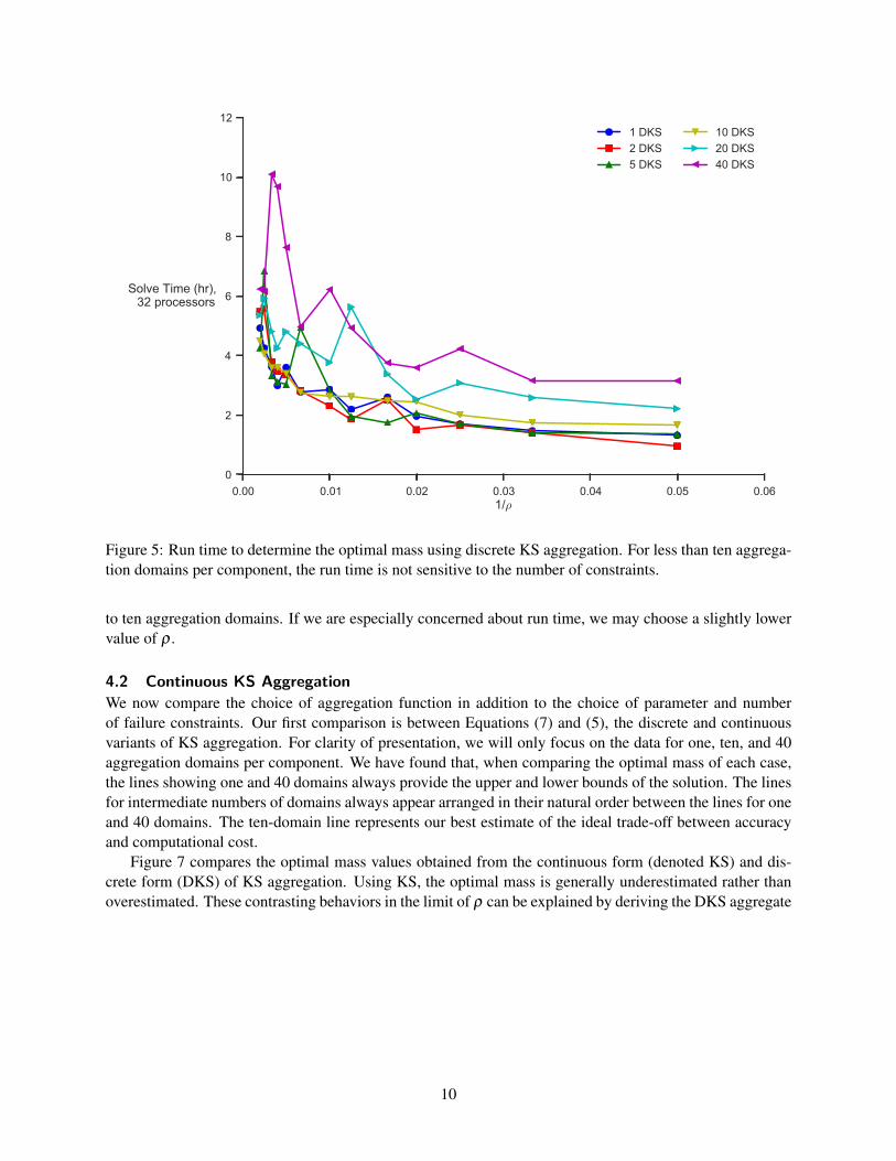
An issue that arises with increasing the number of constraints is the computational cost of the optimiza-tion. In particular, the cost of computing gradients at each iteration using the adjoint method scales withthe number of constraints. Figure 5 shows the wall time of the optimization for each case presented inFigure 3. As we expect, larger values of ρ lead to longer run times because of the increased curvature ofthe aggregated constraints and the resulting ill-conditioning in the optimization problem. For ρ ≥ 200, runtime begins to rise rapidly. However, Figure 5 also suggests that when the number of constraints is not toolarge (less than ten aggregation domains per component in our problem) the run time is insensitive to thenumber of constraints. The increased cost of evaluating more constraint gradients at each iteration is offsetby a reduction in the number of iterations needed to solve the optimization problem.

The analysis of the solution data to this point suggests that there is a “sweet spot” or ideal trade-offbetween accuracy and computational effort. Figure 6 provides a visualization of that trade-off. It shows thesame run time information as Figure 5, but plotted against the optimal mass instead of ρ . Treating Figure 6as a solution plot for a multiobjective problem, we see that the ideal trade-off occurs using ρ ≈ 200 and five

9

0.00 0.01 0.02 0.03 0.04 0.05 0.061/ρ

0

2

4

6

8

10

12

Solve Time (hr),32 processors

1 DKS2 DKS5 DKS

10 DKS20 DKS40 DKS

Figure 5: Run time to determine the optimal mass using discrete KS aggregation. For less than ten aggrega-tion domains per component, the run time is not sensitive to the number of constraints.

to ten aggregation domains. If we are especially concerned about run time, we may choose a slightly lowervalue of ρ .

4.2 Continuous KS Aggregation

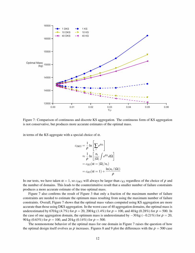
We now compare the choice of aggregation function in addition to the choice of parameter and numberof failure constraints. Our first comparison is between Equations (7) and (5), the discrete and continuousvariants of KS aggregation. For clarity of presentation, we will only focus on the data for one, ten, and 40aggregation domains per component. We have found that, when comparing the optimal mass of each case,the lines showing one and 40 domains always provide the upper and lower bounds of the solution. The linesfor intermediate numbers of domains always appear arranged in their natural order between the lines for oneand 40 domains. The ten-domain line represents our best estimate of the ideal trade-off between accuracyand computational cost.

Figure 7 compares the optimal mass values obtained from the continuous form (denoted KS) and dis-crete form (DKS) of KS aggregation. Using KS, the optimal mass is generally underestimated rather thanoverestimated. These contrasting behaviors in the limit of ρ can be explained by deriving the DKS aggregate

10

14200 14300 14400 14500 14600 14700Optimal Mass (kg)

0

2

4

6

8

10

12

Solve Time (hr),32 processors

1 DKS2 DKS5 DKS

10 DKS20 DKS40 DKS

Figure 6: Trade-off between run time and computed optimal mass using discrete KS aggregation. Theaggregation scheme that provides the best balance between these objectives uses ρ ≈ 200 and five to tenaggregation domains.

11

0.00 0.01 0.02 0.03 0.04 0.05 0.061/ρ

13500

14000

14500

15000

15500

16000

16500

Optimal Mass(kg)

1 DKS10 DKS40 DKS

1 KS10 KS40 KS

Figure 7: Comparison of continuous and discrete KS aggregation. The continuous form of KS aggregationis not conservative, but produces more accurate estimates of the optimal mass.

in terms of the KS aggregate with a special choice of α .

cDKS =1ρ

ln

[∑

ieρgi

]

≈ 1ρ

ln[

nt

|Ω|

∫eρg dΩ

]= cKS(α = |Ω|/nt)

= cKS(α = 1)+ln(nt/|Ω|)

ρ

In our tests, we have taken α = 1, so cDKS will always be larger than cKS regardless of the choice of ρ andthe number of domains. This leads to the counterintuitive result that a smaller number of failure constraintsproduces a more accurate estimate of the true optimal mass.

Figure 7 also confirms the result of Figure 3 that only a fraction of the maximum number of failureconstraints are needed to estimate the optimum mass resulting from using the maximum number of failureconstraints. Overall, Figure 7 shows that the optimal mass values computed using KS aggregation are moreaccurate than those using DKS aggregation. In the worst case of 40 aggregation domains, the optimal mass isunderestimated by 670 kg (4.7%) for ρ = 20, 200 kg (1.4%) for ρ = 100, and 40 kg (0.28%) for ρ = 500. Inthe case of one aggregation domain, the optimum mass is underestimated by −30 kg (−0.21%) for ρ = 20,90 kg (0.63%) for ρ = 100, and 20 kg (0.14%) for ρ = 500.

The nonmonotone behavior of the optimal mass for one domain in Figure 7 raises the question of howthe optimal design itself evolves as ρ increases. Figures 8 and 9 plot the differences with the ρ = 500 case

12

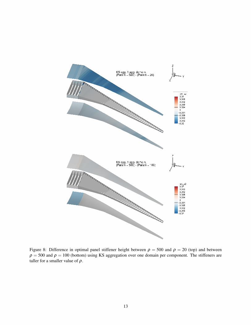
Figure 8: Difference in optimal panel stiffener height between ρ = 500 and ρ = 20 (top) and betweenρ = 500 and ρ = 100 (bottom) using KS aggregation over one domain per component. The stiffeners aretaller for a smaller value of ρ .

13

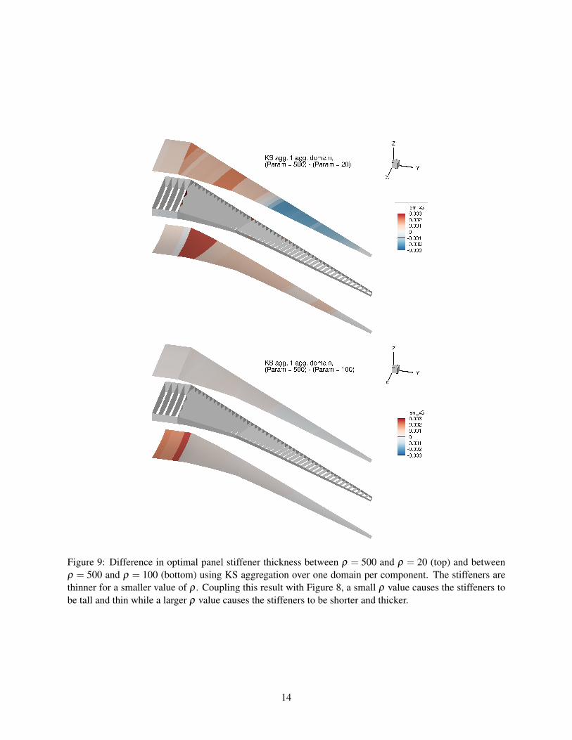
Figure 9: Difference in optimal panel stiffener thickness between ρ = 500 and ρ = 20 (top) and betweenρ = 500 and ρ = 100 (bottom) using KS aggregation over one domain per component. The stiffeners arethinner for a smaller value of ρ . Coupling this result with Figure 8, a small ρ value causes the stiffeners tobe tall and thin while a larger ρ value causes the stiffeners to be shorter and thicker.

14

for two sets of design variables: the stiffener height and the stiffener thickness. As we might expect, thedifferences between the ρ = 500 case and ρ = 100 case are smaller than those between the ρ = 500 andρ = 20 case. However, while the optimum stiffener thickness increases with increasing ρ over much of thewing—indicated by the positive difference value in Figure 9—the optimum stiffener height decreases withincreasing ρ . These two trends have competing influences on the optimal mass; the higher thickness in-creases optimal mass while the lower height decreases optimal mass. Therefore, the nonmonotone behaviorcan be explained by a rapid decrease in stiffener height as ρ increases for a small number of aggregationdomains. When more domains are used, as shown in Figure 10, the difference in optimal height is lower andthe difference in optimal thickness is greater, mitigating the nonmonotone change in optimal mass with ρ .

The run time for obtaining the optimal masses using the KS aggregation is plotted in Figure 11. Theserun times can be directly compared with those obtained using DKS aggregation. Clearly, the run timesobtained using both types of aggregation functions are similar regardless of the number of failure constraints.In terms of the cost-accuracy trade-off, the results in Figures 7 and 11 argue in favor of using KS aggregationin place of DKS aggregation because a more accurate solution can be obtained in a similar computationaltime.

4.3 p-norm Aggregation

As mentioned in Section 2, both the discrete form (8) and the continuous form (6) of p-norm aggregationare only appropriate for failure functions that evaluate to nonnegative values. The buckling constraints inthis problem do not fit that criterion. Tensile loads cause the buckling criterion to become negative andthe absolute value of that negative number can cause a large overestimation of the buckling criterion in theaggregate. Nevertheless, we attempted to use these aggregation schemes in the optimization problems tosee how much progress SNOPT could make from the starting point. In every case, SNOPT terminated afteronly a few minor iterations with the error that it could not satisfy the nonlinear constraints. We interpret thisto mean that the negative values in the buckling criterion caused so much overestimation of the aggregatedbuckling failure that the problem became infeasible. We do not consider the discrete or continuous p-normaggregation strategies further in this study.

4.4 Induced Exponential Aggregation

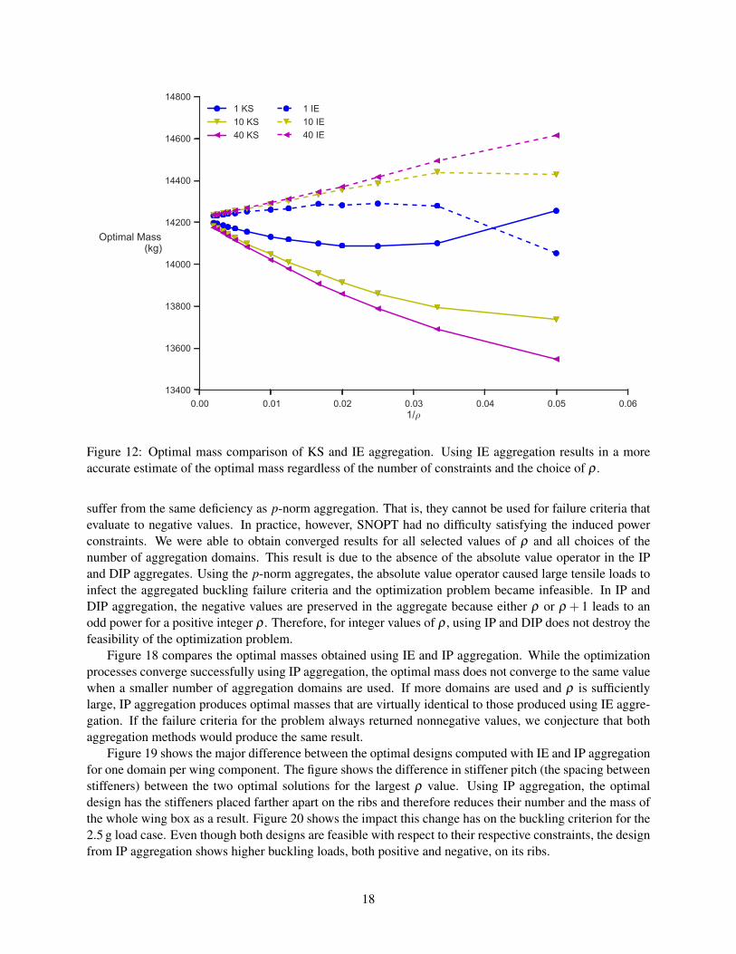
We now directly compare KS aggregation with its induced counterpart, induced exponential aggregation.Figure 12 compares the optimal masses obtained using the continuous form of induced exponential aggre-gation (IE) (9) with those obtained using KS aggregation. Like KS aggregation, we observe that, counter-intuitively, using more IE-aggregated failure constraints reduces the accuracy of the optimal mass estimate.In addition, using more constraints has the advantage of producing a more predictable progression of theoptimal mass as ρ increases. The most interesting feature of Figure 12 is that each optimal mass curve forIE aggregation resembles a reflected version of the corresponding KS aggregation curve. IE aggregationoverestimates the optimal mass where KS aggregation underestimates it, and vice-versa.

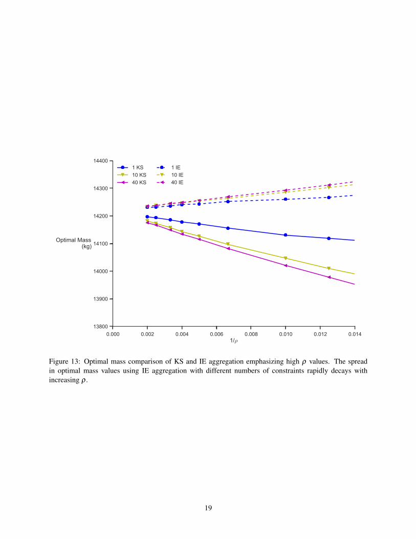
The main advantage of IE aggregation in place of KS aggregation is the rapid decrease in the spreadof optimal mass values with increasing ρ . Figure 13 shows the same data as Figure 12, but focuses on theresults for the largest values of ρ . The optimal mass spread—the difference between the optimal massesof the one domain and 40 domain tests—for ρ = 100 is about 30 kg or 0.21% of the optimal mass. Forρ = 500, the spread is about 5kg or 0.035% of the optimal wing mass. By comparison, the same spreadvalues using KS aggregation are 110 kg (0.77%) and 20 kg (0.14%) respectively. By using IE aggregationin place of KS, the spread has been reduced by 70–75% for large values of ρ . Using IE aggregation withone domain per component, the most accurate in terms of optimal mass, the mass is overestimated by 40 kg(0.28%) for ρ = 100 and 10 kg (0.070%) for ρ = 500. Adding the spread in the optimal mass to the errorin the best case, we see that for ρ ≥ 100 and any number of failure constraints, the maximum error in the

15

Figure 10: Difference in optimal panel stiffener height (top) and thickness (bottom) between ρ = 500 andρ = 20 using KS aggregation and 40 domains per component. The difference in optimal height is smaller,compared to Figure 8, and the difference in optimal thickness is larger, compared to Figure 9, mitigating thenonmonotone behaviour of the optimal mass with changing ρ .

16

0.00 0.01 0.02 0.03 0.04 0.05 0.061/ρ

0

2

4

6

8

10

12

Solve Time (hr),32 processors

1 DKS10 DKS40 DKS

1 KS10 KS40 KS

Figure 11: Run time comparison between KS and DKS aggregation schemes. Both strategies yield similarrun times for the same parameter values and number of domains.

optimal mass is about 1.4% using KS aggregation but only 0.5% using IE aggregation. Therefore, using IEaggregation in place of KS aggregation reduces the error in the optimal mass estimate by more than 60%.

There is a computational price to be paid for this level of accuracy. Figure 14 plots the run time requiredto solve the optimization problems for each case displayed in Figures 12 and 13. Regardless of the choice ofρ and the number of constraints used, the problems that used IE aggregation required much more computa-tional effort. Both aggregation methods used the same quadrature scheme to evaluate the failure constraints,so this increase in effort must be caused by the difficulty of solving the optimization problem, i.e., the num-ber of major iterations taken by SNOPT. This result suggests that robust optimization algorithms are neededin order to use IE aggregation reliably.

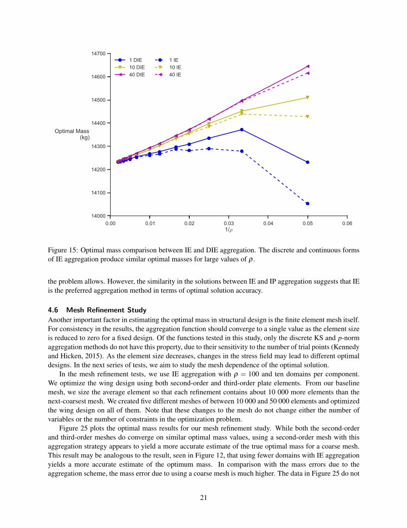
Figures 15 and 16 compare the optimal masses obtained between the continuous and discrete (DIE) (11)forms of induced exponential aggregation. For small values of ρ and a small number of aggregation domains,there is a significant difference between the optimal mass values. Furthermore, the spread in optimal massis much higher using DIE aggregation than using IE aggregation. However, as both ρ and the number ofaggregation domains increases, the difference in optimal mass decreases rapidly. For ρ ≥ 100, both thecontinuous and discrete forms yield nearly identical results.

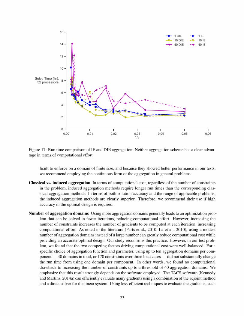
Figure 17 compares the run times of IE and DIE. While there is significant noise in the data, (most likelydue to variations in the optimal search path,) neither aggregation method reliably computes the optimalsolution in less time than the other. Our recommendation, therefore, is to use the continuous form of IEaggregation over the discrete form because of the smaller spread in the optimal mass value discussed above.

4.5 Induced Power Aggregation

In principle, the continuous (IP) (10) and discrete (DIP) (12) forms of induced power aggregation should

17

0.00 0.01 0.02 0.03 0.04 0.05 0.061/ρ

13400

13600

13800

14000

14200

14400

14600

14800

Optimal Mass(kg)

1 KS10 KS40 KS

1 IE10 IE40 IE

Figure 12: Optimal mass comparison of KS and IE aggregation. Using IE aggregation results in a moreaccurate estimate of the optimal mass regardless of the number of constraints and the choice of ρ .

suffer from the same deficiency as p-norm aggregation. That is, they cannot be used for failure criteria thatevaluate to negative values. In practice, however, SNOPT had no difficulty satisfying the induced powerconstraints. We were able to obtain converged results for all selected values of ρ and all choices of thenumber of aggregation domains. This result is due to the absence of the absolute value operator in the IPand DIP aggregates. Using the p-norm aggregates, the absolute value operator caused large tensile loads toinfect the aggregated buckling failure criteria and the optimization problem became infeasible. In IP andDIP aggregation, the negative values are preserved in the aggregate because either ρ or ρ + 1 leads to anodd power for a positive integer ρ . Therefore, for integer values of ρ , using IP and DIP does not destroy thefeasibility of the optimization problem.

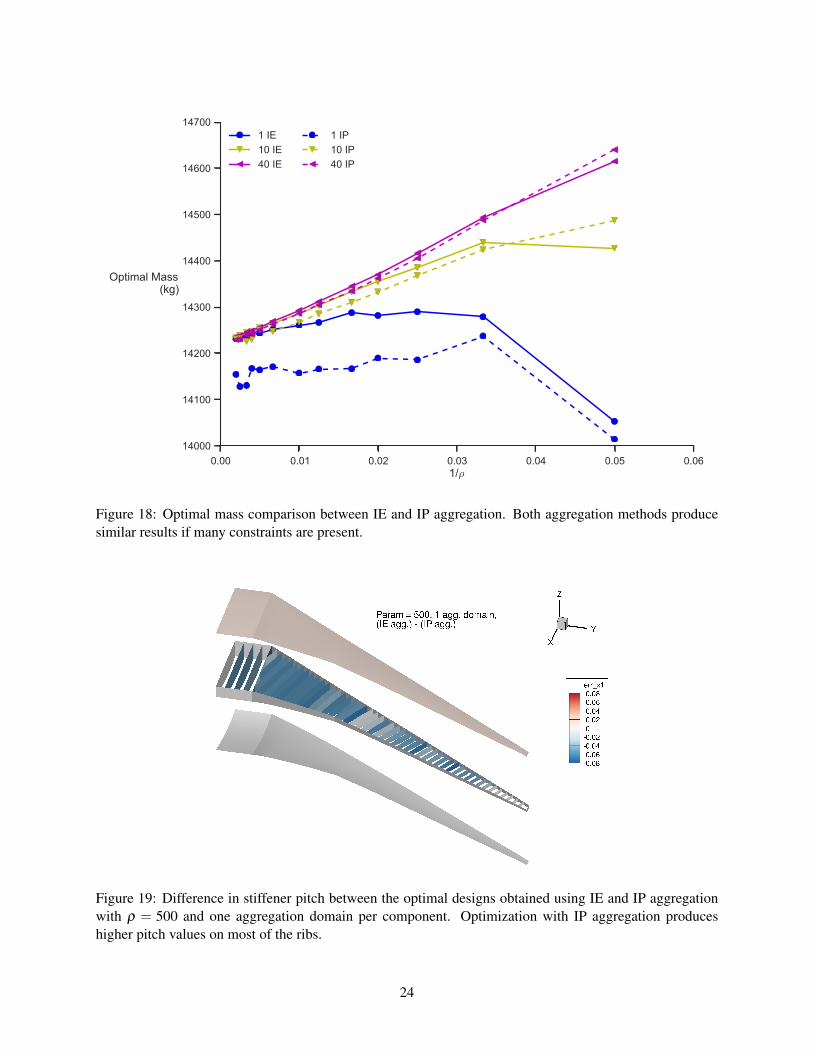
Figure 18 compares the optimal masses obtained using IE and IP aggregation. While the optimizationprocesses converge successfully using IP aggregation, the optimal mass does not converge to the same valuewhen a smaller number of aggregation domains are used. If more domains are used and ρ is sufficientlylarge, IP aggregation produces optimal masses that are virtually identical to those produced using IE aggre-gation. If the failure criteria for the problem always returned nonnegative values, we conjecture that bothaggregation methods would produce the same result.

Figure 19 shows the major difference between the optimal designs computed with IE and IP aggregationfor one domain per wing component. The figure shows the difference in stiffener pitch (the spacing betweenstiffeners) between the two optimal solutions for the largest ρ value. Using IP aggregation, the optimaldesign has the stiffeners placed farther apart on the ribs and therefore reduces their number and the mass ofthe whole wing box as a result. Figure 20 shows the impact this change has on the buckling criterion for the2.5 g load case. Even though both designs are feasible with respect to their respective constraints, the designfrom IP aggregation shows higher buckling loads, both positive and negative, on its ribs.

18

0.000 0.002 0.004 0.006 0.008 0.010 0.012 0.0141/ρ

13800

13900

14000

14100

14200

14300

14400

Optimal Mass(kg)

1 KS10 KS40 KS

1 IE10 IE40 IE

Figure 13: Optimal mass comparison of KS and IE aggregation emphasizing high ρ values. The spreadin optimal mass values using IE aggregation with different numbers of constraints rapidly decays withincreasing ρ .

19

0.00 0.01 0.02 0.03 0.04 0.05 0.061/ρ

0

2

4

6

8

10

12

14

Solve Time (hr),32 processors

1 KS10 KS40 KS

1 IE10 IE40 IE

Figure 14: Run time comparison of KS and IE aggregation. Optimizing with IE aggregation is more com-putationally expensive across all values of ρ and any number of constraints.

The presence of both positive and negative values of the buckling criterion on the wing ribs in Figure 20explains why IE and IP aggregation yield optimal designs that differ only on the wing ribs. On both skins andthe wing spars, the stresses are either all tensile or all compressive so the aggregation of these stresses willnecessarily be tensile or compressive. On the ribs, however, there is a mixture of tensile and compressivestresses. Integrating the failure criterion over the domain causes these stresses to cancel each other out inthe aggregate. This effect can result in a local violation of the buckling constraint that is not picked up bythe aggregate, regardless of the quadrature scheme used to evaluate the integral. Figure 21 clearly showsthis local violation of the buckling constraints. Note that this cancellation phenomenon cannot occur inIE aggregation because the exponential term prevents it. As the number of aggregation domains increases,there is less opportunity for mixed loading to occur in a given aggregation domain, and the optimal designsfrom IP and IE aggregation move into agreement. While this analysis demonstrates that IP aggregation ismore robust than p-norm aggregation, in that it is less likely to lead to an infeasible problem, it is still notas robust as IE aggregation in its handling of negative values of failure criteria.

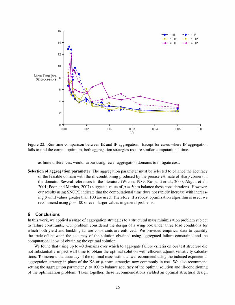
Figure 22 compares the run times for IE and IP aggregation. Generally, the run times using the twodifferent aggregation strategies are similar. The main exception is the case of one aggregation domain andlarge values of ρ . However, we attribute this behavior to the difficulty of handling the mixed loading in theribs using IP aggregation. Using more domains mitigates these ill effects and produces run times similar tothose found with IE aggregation.

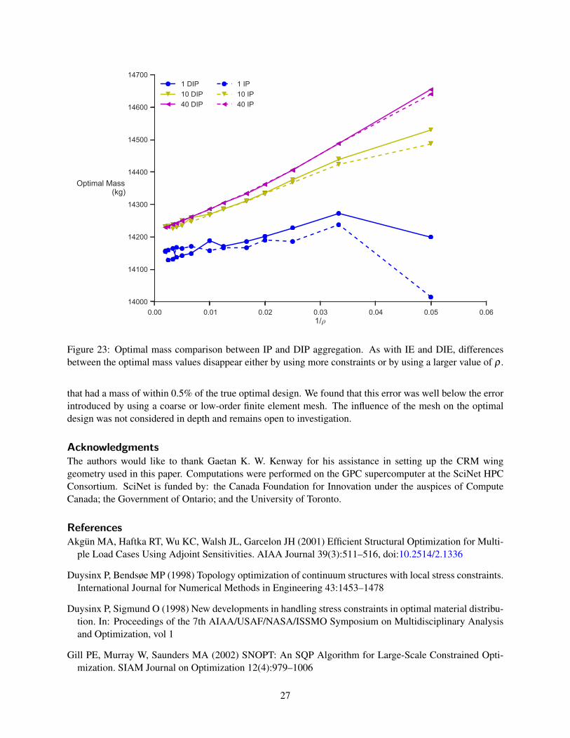
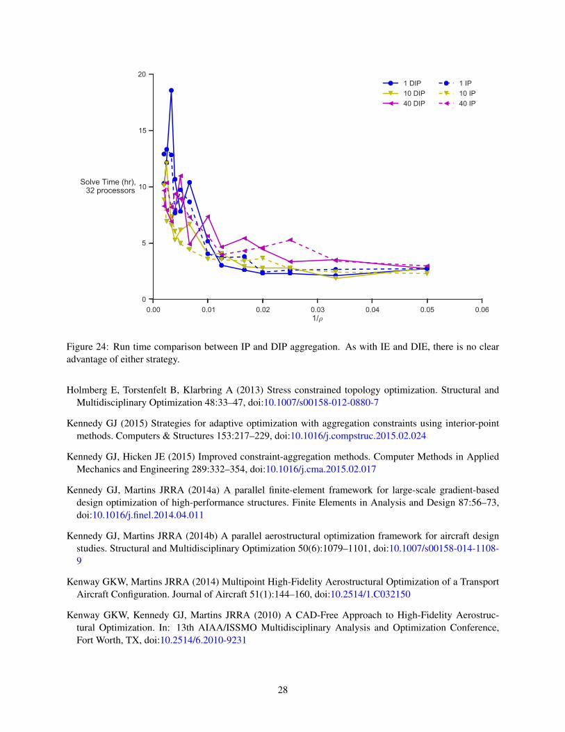
As with IE and DIE aggregation, the differences in the results observed between IP and DIP aggregationare minute when large values of ρ and many aggregation domains are used. Figure 23 compares the optimalmass values while Figure 24 compares run time. Because the error in the optimal mass is smaller for thesame computational effort, we recommend using IP aggregation in place of DIP aggregation in general, if

20

0.00 0.01 0.02 0.03 0.04 0.05 0.061/ρ

14000

14100

14200

14300

14400

14500

14600

14700

Optimal Mass(kg)

1 DIE10 DIE40 DIE

1 IE10 IE40 IE

Figure 15: Optimal mass comparison between IE and DIE aggregation. The discrete and continuous formsof IE aggregation produce similar optimal masses for large values of ρ .

the problem allows. However, the similarity in the solutions between IE and IP aggregation suggests that IEis the preferred aggregation method in terms of optimal solution accuracy.

4.6 Mesh Refinement Study

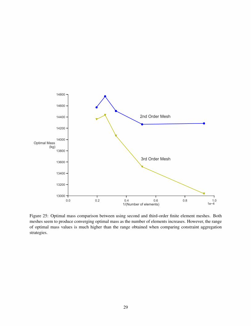
Another important factor in estimating the optimal mass in structural design is the finite element mesh itself.For consistency in the results, the aggregation function should converge to a single value as the element sizeis reduced to zero for a fixed design. Of the functions tested in this study, only the discrete KS and p-normaggregation methods do not have this property, due to their sensitivity to the number of trial points (Kennedyand Hicken, 2015). As the element size decreases, changes in the stress field may lead to different optimaldesigns. In the next series of tests, we aim to study the mesh dependence of the optimal solution.

In the mesh refinement tests, we use IE aggregation with ρ = 100 and ten domains per component.We optimize the wing design using both second-order and third-order plate elements. From our baselinemesh, we size the average element so that each refinement contains about 10 000 more elements than thenext-coarsest mesh. We created five different meshes of between 10 000 and 50 000 elements and optimizedthe wing design on all of them. Note that these changes to the mesh do not change either the number ofvariables or the number of constraints in the optimization problem.

Figure 25 plots the optimal mass results for our mesh refinement study. While both the second-orderand third-order meshes do converge on similar optimal mass values, using a second-order mesh with thisaggregation strategy appears to yield a more accurate estimate of the true optimal mass for a coarse mesh.This result may be analogous to the result, seen in Figure 12, that using fewer domains with IE aggregationyields a more accurate estimate of the optimum mass. In comparison with the mass errors due to theaggregation scheme, the mass error due to using a coarse mesh is much higher. The data in Figure 25 do not

21

0.000 0.002 0.004 0.006 0.008 0.010 0.012 0.014 0.0161/ρ

14000

14100

14200

14300

14400

14500

14600

Optimal Mass(kg)

1 DIE10 DIE40 DIE

1 IE10 IE40 IE

Figure 16: Optimal mass comparison between IE and DIE aggregation focusing on large values of ρ . Forρ ≥ 100, the two aggregation functions produce virtually identical results.

point to a clear estimate of the true optimal mass, but the optimal mass computed by the second order meshfalls in a 600-kg range of values. The optimal mass computed by the third order mesh falls in a 1400-kg rangeof values. By comparison, the range of mass values displayed in Figure 12 for every IE aggregation schemeis less than 500 kg. If we only consider ρ ≥ 100, the range of mass values is less than 100 kg. These resultsall suggest that the choice of mesh can be even more important than the choice of constraint aggregationmethod for obtaining an accurate optimal mass estimate in stress-constrained structural optimization.

5 Discussion and RecommendationsOur study is fundamentally limited to one large structural optimization problem. Because of the smearedstiffness model employed in the structural analysis, multiple variables on each panel could be used to in-crease the apparent stiffness of that panel. We found that this resulted in multiple local minima on thisoptimization problem when only yield stress failure was constrained. Therefore, we are not able to com-pare the KS and p-norm aggregation directly or to compare p-norm with IP aggregation directly. We couldmix the aggregation types in a single problem, such as using KS functions for the buckling failure and p-norm functions for the yield stress failure, but have not done so to better study the aggregation methodsthemselves.

With the above limitation in mind, we present some general recommendations for employing constraintaggregation based on our results.

Continuous vs. discrete aggregation While some discrete aggregation methods are conservative with re-spect to failure at prescribed points in the domain, they also exhibit mesh-dependence and produceless accurate estimates of the true optimum mass compared to their continuous analogues. Theseproperties are especially evident when a small value of ρ is chosen. Because conservatism is so dif-

22

0.00 0.01 0.02 0.03 0.04 0.05 0.061/ρ

0

2

4

6

8

10

12

14

16

Solve Time (hr),32 processors

1 DIE10 DIE40 DIE

1 IE10 IE40 IE

Figure 17: Run time comparison of IE and DIE aggregation. Neither aggregation scheme has a clear advan-tage in terms of computational effort.

ficult to enforce on a domain of finite size, and because they showed better performance in our tests,we recommend employing the continuous form of the aggregation in general problems.

Classical vs. induced aggregation In terms of computational cost, regardless of the number of constraintsin the problem, induced aggregation methods require longer run times than the corresponding clas-sical aggregation methods. In terms of both solution accuracy and the range of applicable problems,the induced aggregation methods are clearly superior. Therefore, we recommend their use if highaccuracy in the optimal design is required.

Number of aggregation domains Using more aggregation domains generally leads to an optimization prob-lem that can be solved in fewer iterations, reducing computational effort. However, increasing thenumber of constraints increases the number of gradients to be computed at each iteration, increasingcomputational effort. As noted in the literature (Parıs et al., 2010; Le et al., 2010), using a modestnumber of aggregation domains instead of a large number can greatly reduce computational cost whileproviding an accurate optimal design. Our study reconfirms this practice. However, in our test prob-lem, we found that the two competing factors driving computational cost were well-balanced. For aspecific choice of aggregation function and parameter, using up to ten aggregation domains per com-ponent — 40 domains in total, or 170 constraints over three load cases — did not substantially changethe run time from using one domain per component. In other words, we found no computationaldrawback to increasing the number of constraints up to a threshold of 40 aggregation domains. Weemphasize that this result strongly depends on the software employed. The TACS software (Kennedyand Martins, 2014a) can efficiently evaluate many gradients using a combination of the adjoint methodand a direct solver for the linear system. Using less-efficient techniques to evaluate the gradients, such

23

0.00 0.01 0.02 0.03 0.04 0.05 0.061/ρ

14000

14100

14200

14300

14400

14500

14600

14700

Optimal Mass(kg)

1 IE10 IE40 IE

1 IP10 IP40 IP

Figure 18: Optimal mass comparison between IE and IP aggregation. Both aggregation methods producesimilar results if many constraints are present.

Figure 19: Difference in stiffener pitch between the optimal designs obtained using IE and IP aggregationwith ρ = 500 and one aggregation domain per component. Optimization with IP aggregation produceshigher pitch values on most of the ribs.

24

Figure 20: Comparison of buckling criterion values between optimal designs obtained using IE and IPaggregation with ρ = 500 and one aggregation domain per component. The ribs are the only part of thewing structure where we observe a mixture of tensile and compressive loads.

Figure 21: Same data as Figure 20, but focused on the ribs. The high positive values of the buckling criterionobserved on some ribs of the IP optimum are infeasible with respect to the IE constraints. In the aggregation,however, they are offset by the high negative values observed on ribs near the wing root.

25

0.00 0.01 0.02 0.03 0.04 0.05 0.061/ρ

0

2

4

6

8

10

12

14

16

Solve Time (hr),32 processors

1 IE10 IE40 IE

1 IP10 IP40 IP

Figure 22: Run time comparison between IE and IP aggregation. Except for cases where IP aggregationfails to find the correct optimum, both aggregation strategies require similar computational time.

as finite differences, would favour using fewer aggregation domains to mitigate cost.

Selection of aggregation parameter The aggregation parameter must be selected to balance the accuracyof the feasible domain with the ill-conditioning produced by the precise estimate of sharp corners inthe domain. Several references in the literature (Wrenn, 1989; Raspanti et al., 2000; Akgun et al.,2001; Poon and Martins, 2007) suggest a value of ρ = 50 to balance these considerations. However,our results using SNOPT indicate that the computational time does not rapidly increase with increas-ing ρ until values greater than 100 are used. Therefore, if a robust optimization algorithm is used, werecommend using ρ = 100 or even larger values in general problems.

6 ConclusionsIn this work, we applied a range of aggregation strategies to a structural mass minimization problem subjectto failure constraints. Our problem considered the design of a wing box under three load conditions forwhich both yield and buckling failure constraints are enforced. We provided empirical data to quantifythe trade-off between the accuracy of the solution obtained using aggregated failure constraints and thecomputational cost of obtaining the optimal solution.

We found that using up to 40 domains over which to aggregate failure criteria on our test structure didnot substantially impact wall time to obtain the optimal solution with efficient adjoint sensitivity calcula-tions. To increase the accuracy of the optimal mass estimate, we recommend using the induced exponentialaggregation strategy in place of the KS or p-norm strategies now commonly in use. We also recommendsetting the aggregation parameter ρ to 100 to balance accuracy of the optimal solution and ill-conditioningof the optimization problem. Taken together, these recommendations yielded an optimal structural design

26

0.00 0.01 0.02 0.03 0.04 0.05 0.061/ρ

14000

14100

14200

14300

14400

14500

14600

14700

Optimal Mass(kg)

1 DIP10 DIP40 DIP

1 IP10 IP40 IP

Figure 23: Optimal mass comparison between IP and DIP aggregation. As with IE and DIE, differencesbetween the optimal mass values disappear either by using more constraints or by using a larger value of ρ .

that had a mass of within 0.5% of the true optimal design. We found that this error was well below the errorintroduced by using a coarse or low-order finite element mesh. The influence of the mesh on the optimaldesign was not considered in depth and remains open to investigation.

AcknowledgmentsThe authors would like to thank Gaetan K. W. Kenway for his assistance in setting up the CRM winggeometry used in this paper. Computations were performed on the GPC supercomputer at the SciNet HPCConsortium. SciNet is funded by: the Canada Foundation for Innovation under the auspices of ComputeCanada; the Government of Ontario; and the University of Toronto.

ReferencesAkgun MA, Haftka RT, Wu KC, Walsh JL, Garcelon JH (2001) Efficient Structural Optimization for Multi-

ple Load Cases Using Adjoint Sensitivities. AIAA Journal 39(3):511–516, doi:10.2514/2.1336

Duysinx P, Bendsøe MP (1998) Topology optimization of continuum structures with local stress constraints.International Journal for Numerical Methods in Engineering 43:1453–1478

Duysinx P, Sigmund O (1998) New developments in handling stress constraints in optimal material distribu-tion. In: Proceedings of the 7th AIAA/USAF/NASA/ISSMO Symposium on Multidisciplinary Analysisand Optimization, vol 1

Gill PE, Murray W, Saunders MA (2002) SNOPT: An SQP Algorithm for Large-Scale Constrained Opti-mization. SIAM Journal on Optimization 12(4):979–1006

27

0.00 0.01 0.02 0.03 0.04 0.05 0.061/ρ

0

5

10

15

20

Solve Time (hr),32 processors

1 DIP10 DIP40 DIP

1 IP10 IP40 IP

Figure 24: Run time comparison between IP and DIP aggregation. As with IE and DIE, there is no clearadvantage of either strategy.

Holmberg E, Torstenfelt B, Klarbring A (2013) Stress constrained topology optimization. Structural andMultidisciplinary Optimization 48:33–47, doi:10.1007/s00158-012-0880-7

Kennedy GJ (2015) Strategies for adaptive optimization with aggregation constraints using interior-pointmethods. Computers & Structures 153:217–229, doi:10.1016/j.compstruc.2015.02.024

Kennedy GJ, Hicken JE (2015) Improved constraint-aggregation methods. Computer Methods in AppliedMechanics and Engineering 289:332–354, doi:10.1016/j.cma.2015.02.017

Kennedy GJ, Martins JRRA (2014a) A parallel finite-element framework for large-scale gradient-baseddesign optimization of high-performance structures. Finite Elements in Analysis and Design 87:56–73,doi:10.1016/j.finel.2014.04.011

Kennedy GJ, Martins JRRA (2014b) A parallel aerostructural optimization framework for aircraft designstudies. Structural and Multidisciplinary Optimization 50(6):1079–1101, doi:10.1007/s00158-014-1108-9

Kenway GKW, Martins JRRA (2014) Multipoint High-Fidelity Aerostructural Optimization of a TransportAircraft Configuration. Journal of Aircraft 51(1):144–160, doi:10.2514/1.C032150

Kenway GKW, Kennedy GJ, Martins JRRA (2010) A CAD-Free Approach to High-Fidelity Aerostruc-tural Optimization. In: 13th AIAA/ISSMO Multidisciplinary Analysis and Optimization Conference,Fort Worth, TX, doi:10.2514/6.2010-9231

28

0.0 0.2 0.4 0.6 0.8 1.01/(Number of elements) 1e 4

13000

13200

13400

13600

13800

14000

14200

14400

14600

14800

Optimal Mass(kg)

2nd Order Mesh

3rd Order Mesh

Figure 25: Optimal mass comparison between using second and third-order finite element meshes. Bothmeshes seem to produce converging optimal mass as the number of elements increases. However, the rangeof optimal mass values is much higher than the range obtained when comparing constraint aggregationstrategies.

29

0.0 0.2 0.4 0.6 0.8 1.01/(Number of elements) 1e 4

0

5

10

15

20

Solve Time (hr),32 processors

2nd Order Mesh

3rd Order Mesh

Figure 26: Run time comparison between second and third-order finite element meshes. Not surprisingly,using a lower-order mesh greatly reduces computational effort.

Kenway GKW, Kennedy GJ, Martins JRRA (2014a) Aerostructural optimization of the Common Re-search Model configuration. 15th AIAA/ISSMO Multidisciplinary Analysis and Optimization Conferencedoi:10.2514/6.2014-3274

Kenway GKW, Kennedy GJ, Martins JRRA (2014b) Scalable Parallel Approach for High-FidelitySteady-State Aeroelastic Analysis and Adjoint Derivative Computations. AIAA Journal 52(5):935–951,doi:10.2514/1.J052255

Kreisselmeier G, Steinhauser R (1979) Systematic Control Design by Optimizing a Vector PerformanceIndicator. In: Symposium on Computer-Aided Design of Control Systems, IFAC, Zurich, Switzerland,pp 113–117

Kreisselmeier G, Steinhauser R (1983) Application of Vector Performance Optimization to a Ro-bust Control Loop Design for a Fighter Aircraft. International Journal of Control 37(2):251–284,doi:10.1080/00207179.1983.9753066

Lambe AB, Martins JRRA (2015) Matrix-Free Aerostructural Optimization of Aircraft Wings. Structuraland Multidisciplinary Optimization

Le C, Norato J, Bruns T, Ha C, Tortorelli D (2010) Stress-based topology optimization for continua. Struc-tural and Multidisciplinary Optimization 41(4):605–620, doi:10.1007/s00158-009-0440-y

Lyu Z, Kenway GKW, Martins JRRA (2014) Aerodynamic Shape Optimization Investigations of the Com-mon Research Model Wing Benchmark. AIAA Journal 53(4):968–985, doi:10.2514/6.2014-0567

30

Parıs J, Navarrina F, Colominas I, Casteleiro M (2009) Topology optimization of continuum structureswith local and global stress constraints. Structural and Multidisciplinary Optimization 39:419–437,doi:10.1007/s00158-008-0336-2

Parıs J, Navarrina F, Colominas I, Casteleiro M (2010) Block aggregation of stress con-straints in topology optimization of structures. Advances in Engineering Software 41:433–441,doi:10.1016/j.advengsoft.2009.03.006

Perez RE, Jansen PW, Martins JRRA (2012) pyOpt: A Python-Based Object-Oriented Framework forNonlinear Constrained Optimization. Structural and Multidisciplinary Optimization 45(1):101–118,doi:10.1007/s00158-011-0666-3

Poon NMK, Martins JRRA (2007) An adaptive approach to constraint aggregation using adjoint sensitivityanalysis. Structural and Multidisciplinary Optimization 34:61–73, doi:10.1007/s00158-006-0061-7

Qiu GY, Li XS (2010) A note on the derivation of global stress constraints. Structural and MultidisciplinaryOptimization 40:625–628, doi:10.1007/s00158-009-0397-x

Raspanti CG, Bandoni JA, Biegler LT (2000) New strategies for flexibility analysis and design under uncer-tainty. Computers & Chemical Engineering 24:2193–2209, doi:10.1016/S0098-1354(00)00591-3

Vassberg JC, DeHaan MA, Rivers SM, Wahls RA (2008) Development of a Common Research Model forapplied CFD validation studies. AIAA 2008-6919

van der Weide E, Kalitzin G, Schluter J, Alonso J (2006) Unsteady Turbomachinery Computations Us-ing Massively Parallel Platforms. In: 44th AIAA Aerospace Sciences Meeting and Exhibit, AerospaceSciences Meetings, American Institute of Aeronautics and Astronautics, doi:doi:10.2514/6.2006-421

Wrenn GA (1989) An Indirect Method for Numerical Optimization Using the Kreisselmeier–SteinhauserFunction. Tech. rep., NASA Langley Research Center, Hampton, VA

31