An essay on assignment games - Universitat de Barcelona
57
GRAU DE MATEMÀTIQUES Facultat de Matemàtiques i Informàtica Universitat de Barcelona DEGREE PROJECT An essay on assignment games Rubén Ureña Martínez Advisor: Dr. Javier Martínez de Albéniz Dept. de Matemàtica Econòmica, Financera i Actuarial Barcelona, January 2017
Transcript of An essay on assignment games - Universitat de Barcelona
GRAU DE MATEMÀTIQUES
Facultat de Matemàtiques i InformàticaUniversitat de Barcelona
DEGREE PROJECT
An essay on assignment games
Rubén Ureña Martínez
Advisor: Dr. Javier Martínez de AlbénizDept. de Matemàtica Econòmica, Financera i Actuarial
Barcelona, January 2017

Abstract
This degree project studies the main results on the bilateral assignment game. This isa part of cooperative game theory and models a market with indivisibilities and money.There are two sides of the market, let us say buyers and sellers, or workers and firms, suchthat when we match two agents from different sides, a profit is made.
We show some good properties of the core of these games, such as its non-emptiness andits lattice structure. There are two outstanding points: the buyers-optimal core allocationand the sellers-optimal core allocation, in which all agents of one sector get their bestpossible outcome.
We also study a related non-cooperative mechanism, an auction, to implement the buyers-optimal core allocation.
Resumen
Este trabajo de fin de grado estudia los resultados principales acerca de los juegos deasignación bilaterales. Corresponde a una parte de la teoría de juegos cooperativos yproporciona un modelo de mercado con indivisibilidades y dinero. Hay dos lados delmercado, digamos compradores y vendedores, o trabajadores y empresas, de manera quecuando se emparejan dos agentes de distinto lado, se produce un cierto beneficio.
Se muestran además algunas buenas propiedades del núcleo de estos juegos, tales como sucondición de ser siempre no vacío y su estructura de retículo. Encontramos dos puntosdestacados: la distribución óptima para los compradores en el núcleo y la distribuciónóptima para los vendedores en el núcleo, en las cuales todos los agentes de cada sectorobtienen simultáneamente el mejor resultado posible en el núcleo.
También estudiamos un mecanismo no cooperativo, una subasta, para implementar ladistribución óptima para los compradores en el núcleo.

Contents
Abstract iii
Contents v
1 Introduction 1
2 Cooperative games 52.1 Introduction to cooperative games . . . . . . . . . . . . . . . . . . . . . . . 52.2 The core and related concepts . . . . . . . . . . . . . . . . . . . . . . . . . . 8
3 Assignment problems and linear programming 113.1 Assignment problems . . . . . . . . . . . . . . . . . . . . . . . . . . . . . . . 113.2 Linear programming . . . . . . . . . . . . . . . . . . . . . . . . . . . . . . . 13
4 Assignment games 214.1 The assignment model . . . . . . . . . . . . . . . . . . . . . . . . . . . . . . 214.2 The assignment game . . . . . . . . . . . . . . . . . . . . . . . . . . . . . . 224.3 The core of the assignment game . . . . . . . . . . . . . . . . . . . . . . . . 254.4 Lattice structure of the core of the assignment game . . . . . . . . . . . . . 304.5 Buyer and seller optima . . . . . . . . . . . . . . . . . . . . . . . . . . . . . 354.6 The extreme core allocations of the assignment game . . . . . . . . . . . . . 364.7 Some single-valued solutions . . . . . . . . . . . . . . . . . . . . . . . . . . . 41
5 Multi-item auctions 435.1 Multi-item auction mechanism . . . . . . . . . . . . . . . . . . . . . . . . . 43
6 Conclusions 47
Bibliography 49

Chapter 1
Introduction
This degree project covers the study of assignment problems in a game theoretical frame-work, focusing on assignment games and especially in stability notions, that is the core.
What is game theory about?
Decisions are made every day, by all type of agents, let it be individual persons, firms,governments or any kind of economic agent. The outcomes of the decision do not onlydepend on the decision of the agent but also on the decisions of others. Therefore GameTheory is a formal approach (mathematical in form) to analyze the process of decisionmaking of several agents in mutually dependent situations.
Von Neumann and Morgenstern (1944) [42] introduces for the first time the term GameTheory in their book “Theory of Games and Economic Behavior”. They distinguish in thisbook two major approaches, non-cooperative game theory and cooperative game theory.
Nash (1951) [23] defines the difference in between the two approaches that in a non-cooperative game “each participant acts independently, without collaboration or commu-nication with any of the others”, while in a cooperative game they “may communicate andform coalitions which will be enforced by an umpire”, and also “this theory is based on ananalysis of the interrelationships of the various coalitions which can be formed by the play-ers of the game”. While non-cooperative game theory deals with situations with possiblyopposing interests and which actions agents would choose in such situations, cooperativegame theory is concerned with what kinds of coalitions would be formed and how muchpayoff every agent should receive.
A cooperative game with transferable utility, or simply a TU-game, considers the situationin which agents are able to cooperate to form coalitions and the total payoff obtained fromtheir cooperation can be freely distributed among the agents in the coalition.
More precisely, a TU-game is described by a finite set of agents, called players, and acharacteristic function. A characteristic function of a TU-game assigns to each coalitionthe total profit, or worth, which can be obtained by the coalition without cooperating withplayers outside the coalition. A fundamental question of TU-games is how much payoff
1
INTRODUCTION 2
each player must receive.
A solution concept for TU-games assigns to each TU-game a set of allocations that satisfycertain properties, or axioms. One of the well-known solution concepts of TU-games is thecore introduced by Gillies (1959) [13], as the set of allocations that are efficient and exactlydistribute the worth of the grand coalition of all players, and are stable in the sense thatno group of players has the incentive to leave the grand coalition and obtain the worth ofthemselves.
Assignment problems and assignment games
One of the earliest works on assignment problems within an economic context is Koopmansand Beckmann (1957) [16]. The authors study a market situation in which industrial plantshad to be assigned to the designated locations. The idea is to match two disjoint sets(plants and locations) by mixed-pairs where each possible mixed-pair has a given value.The problem in this context is to find a matching with the highest total valuation of mixed-pairs. Making use of Birkhoff-von Neumann Theorem (Birkhoff (1946) [2]; von Neumann(1953) [43]), they show that an optimal assignment can be obtained by solving a linearprogram. Furthermore, they introduce a system of rents (prices) on the locations thatsustain the optimal assignment by solving the dual linear program. Related to that, Gale(1960) [11] defines competitive equilibrium prices and shows they exist for any assignmentproblem.
Shapley and Shubik (1971) [36] introduces the assignment problem in a cooperative gameframework. The authors study a two-sided (house) market. In their setting, there aretwo disjoint sets that consist of m buyers and n sellers respectively. Each buyer wantsto buy at most one house and each seller has one house on sale. Utility is identified withmoney, each buyer has a value (which can be different) for every house, and each seller has areservation value. The valuation matrix represents the joint profit obtained by each mixed-pair. They define the corresponding cooperative game (assignment game) for the market.The question is how to share the profit and, to this end, the authors analyze a solutionconcept: the core (the set of allocations that cannot be improved upon by any coalition).They show that the core of an assignment game is always non-empty. Furthermore, itcoincides with the set of dual solutions to the assignment problem, also with the set ofcompetitive equilibrium payoff vectors, and has a lattice structure. Demange (1982) [9]and Leonard (1983) [18] prove that in the buyers-optimal core allocation each buyer attainshis/her marginal contribution and in the sellers-optimal core allocation each seller attainshis/her marginal contribution.
This monograph is organized as follows. In Chapter 2, we introduce formally the conceptof cooperative game, and to this end we introduce a short overview of the notion of util-ity and a first distinction between non-transferable utility (NTU) cooperative games andtransferable utility (TU) cooperative games. Besides that, we introduce the core of a gameand several other essential definitions.
In Chapter 3 we discuss the assignment problem as a part of Operations Research. Linearsum assignment problem is the first and most important assignment problem, and imme-diately this connects with linear programming. Therefore, this chapter also presents the
INTRODUCTION 3
linear programming as a mathematical technique going through the most basic notions un-til reaching the duality theorem, which is indispensable to enter into assignment marketsand games.
Next chapter, Chapter 4, is the central core of this dissertation. It introduces the assign-ment market and its associated assignment game. This model of cooperative game wasintroduced by Shapley and Shubik (1971) [36]. We study the model, an outstanding setsolution and the core. We show some good properties of the core of these games, such asits non-emptiness and its lattice structure. We also speak of two outstanding points: thebuyers-optimal core allocation and the sellers-optimal core allocation. Some single-valuedsolutions worthy of mention are the τ -value or fair solution (Thompson, 1981) [39], andthe nucleolus (Schmeidler, 1969) [35].
An assignment market with only one seller is the setting of an auction, either a single-object auction or a multi-item auction, depending on the number of objects on sale by theseller. In the final chapter of this dissertation, Chapter 5, we study an auction, which isa mechanism non-cooperative in nature, to obtain the buyers-optimal core allocation: themulti-item auction.
Some final conclusions end this dissertation.

Chapter 2
Cooperative games
2.1 Introduction to cooperative games
Game theory can be broadly divided in non-cooperative and cooperative game theory. Asopposed to the non-cooperative models, where the main focus is on the strategic aspects ofthe interaction among the players, the approach in cooperative game theory is completelydifferent. Now, it is assumed that players can commit to behave in a way that is sociallyoptimal, and therefore the benefits can be as big as possible. The reason can be a contract,a law or a custom. The main issue is how to share the benefits arising from cooperation.Important elements in this approach are the different subgroups of players, referred toas coalitions, and the set of outcomes that each coalition can get regardless of what theplayers outside the coalition do1. When discussing the different equilibrium concepts fornon-cooperative games, we are concerned about whether a given strategy profile is self-enforcing or not, in the sense that no player has incentives to deviate. We now assume thatplayers can make binding agreements and, hence, instead of being worried about issues likeself-enforceability, we care about notions like fairness and equity.
Utility
In economics, utility is a measure of preferences over some set of goods. The conceptis an important underpinning of rational choice theory in economics and game theory:since one cannot directly measure benefit, satisfaction or happiness from a good or service,economists instead have devised ways of representing and measuring utility in terms of mea-surable economic choices. Economists have attempted to perfect highly abstract methodsof comparing utilities by observing and calculating economic choices; in the simplest sense,economists consider utility to be revealed in people’s willingness to pay different amountsfor different goods.
In fact it is assumed that any agent has preferences over goods (binary relation, complete1In Peleg and Sudhölter (2003, Chapter 11) [30], the authors discuss in detail some relations between
the two approaches and, in particular, they derive the definition of cooperative game without transferableutility (Definition 2.1 below) from a strategic game in which the players are allowed to form coalitions anduse them to coordinate their strategies through binding agreements.
5
CHAPTER 2. COOPERATIVE GAMES 6
and transitive), and if this preference satisfy some assumptions it can be represented byan utility function.
Depending on whether transference of utility between players is restricted or not, we distin-guish between nontransferable utility games (NTU-games) and transferable utility games(TU-games), respectively.
Nontransferable Utility Games
In this section we present a brief introduction to the most general class of cooperativegames: nontransferable utility cooperative games or NTU-games. The main source ofgenerality comes from the fact that, although binding agreements between the players areimplicitly assumed to be possible, utility is not transferable across players. Below, wepresent the formal definition and then we illustrate it with an example.
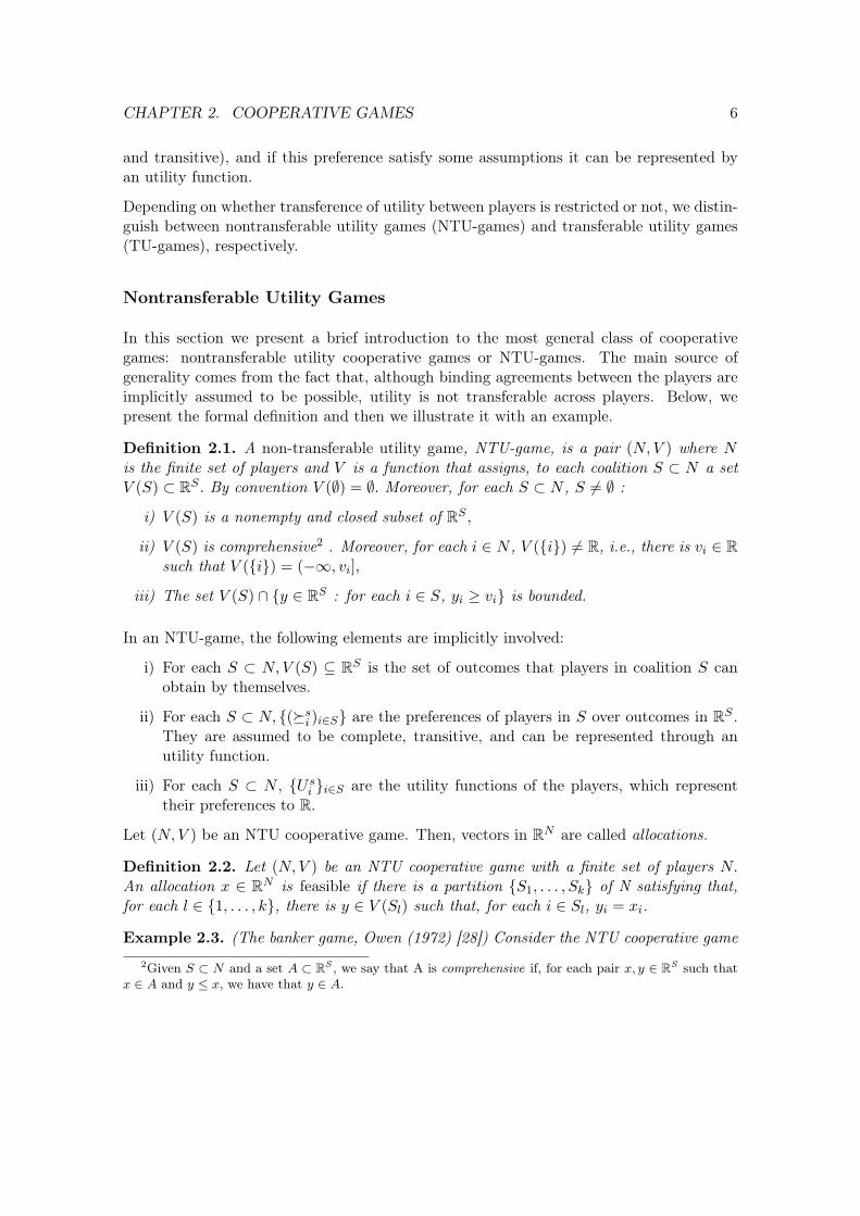
Definition 2.1. A non-transferable utility game, NTU-game, is a pair (N,V ) where Nis the finite set of players and V is a function that assigns, to each coalition S ⊂ N a setV (S) ⊂ RS . By convention V (∅) = ∅. Moreover, for each S ⊂ N , S 6= ∅ :
i) V (S) is a nonempty and closed subset of RS ,
ii) V (S) is comprehensive2 . Moreover, for each i ∈ N , V ({i}) 6= R, i.e., there is vi ∈ Rsuch that V ({i}) = (−∞, vi],
iii) The set V (S) ∩ {y ∈ RS : for each i ∈ S, yi ≥ vi} is bounded.
In an NTU-game, the following elements are implicitly involved:
i) For each S ⊂ N,V (S) ⊆ RS is the set of outcomes that players in coalition S canobtain by themselves.
ii) For each S ⊂ N, {(�si )i∈S} are the preferences of players in S over outcomes in RS .They are assumed to be complete, transitive, and can be represented through anutility function.
iii) For each S ⊂ N , {U si }i∈S are the utility functions of the players, which representtheir preferences to R.
Let (N,V ) be an NTU cooperative game. Then, vectors in RN are called allocations.
Definition 2.2. Let (N,V ) be an NTU cooperative game with a finite set of players N.An allocation x ∈ RN is feasible if there is a partition {S1, . . . , Sk} of N satisfying that,for each l ∈ {1, . . . , k}, there is y ∈ V (Sl) such that, for each i ∈ Sl, yi = xi.
Example 2.3. (The banker game, Owen (1972) [28]) Consider the NTU cooperative game2Given S ⊂ N and a set A ⊂ RS , we say that A is comprehensive if, for each pair x, y ∈ RS such that
x ∈ A and y ≤ x, we have that y ∈ A.
CHAPTER 2. COOPERATIVE GAMES 7
(N,V ) given by:
V ({i}) = {xi : xi ≤ 0}, i ∈ {1, 2, 3},V ({1, 2}) = {(x1, x2) : x1 + 4x2 ≤ 1000, x1 ≤ 1000}V ({1, 3}) = {(x1, x3) : x1 ≤ 0, x3 ≤ 0},V ({2, 3}) = {(x2, x3) : x2 ≤ 0, x3 ≤ 0},V ({N}) = {(x1, x2, x3) : x1 + x2 + x3 ≤ 1000}.
One can think of this game in the following way. On its own, no player can get anything.Player 1, with the help of player 2, can get 1000 dollars. Player 1 can reward player 2by sending him money, but the money sent is lost or stolen with probability 0.75. Player3 is a banker, so player 1 can ensure his transactions are safely delivered to player 2 byusing player 3 as intermediary. Hence, the question is how much should player 1 pay toplayer 2 for his help to get the 1000 dollars and how much to player 3 for helping himto make transactions to player 2 at no cost. The reason for referring to these games asnontransferable utility games is that some transfers among the players may not be allowed.In this example, for instance, (1000, 0) belongs to V ({1, 2}), but players 1 and 2 cannotagree to the share (500, 500) without the help of player 3.
In the next part, we define games with transferable utility, in which all transfers areassumed to be possible.
Transferable Utility Games
We now move to the most widely studied class of cooperative games: those with transferableutility, in short, TU-cooperative games, or TU-games. Here, the different coalitions thatcan be formed among the players in N can enforce certain allocations (possibly throughbinding agreements); the problem is to decide how benefits generated by the cooperationof the players (formation of coalitions) have to be shared among them. However, there isone important departure from the general NTU-games framework.
Definition 2.4. A TU-game is a pair (N, v), where N is the (finite) set of players andv : 2N → R is the characteristic function of the game. By convention, v(∅) := 0.
In general, we interpret v(S), the worth of coalition S, as the benefit that players in Scan generate. When no confusion arises, we denote the game (N, v) by v. Also, we denotev({i}) and v({i, j}) by v(i) and v(ij), respectively. Let GN be the class of TU-games withplayer set N .
Example 2.5. (The glove game, Owen (1975) [29]) Three players are willing to divide thebenefits of selling a pair of gloves. Player 1 has a left glove and players 2 and 3 have oneright glove each. A left-right pair of gloves can be sold for one euro. This situation can bemodeled as the TU-game (N, v), where N = {1, 2, 3}, v(1) = v(2) = v(3) = v(23) = 0, andv(12) = v(13) = v(N) = 1.
Example 2.6. (The Parliament of Aragón, González-Díaz et al. (2010) [14]) In this case,we consider the Parliament of Aragón, one of the regions of Spain. After the electionswhich took place in May 1991, its composition was: PSOE had 30 seats, PP had 17 seats,
CHAPTER 2. COOPERATIVE GAMES 8
PAR had 17 seats, and IU had 3 seats. In a Parliament, the most relevant decisions aremade using the simple majority rule. We can use TU-games to measure the power ofthe different parties in a Parliament. This can be seen as "dividing" the power amongthem. A coalition is said to have the power if it collects more than half of the seats of theParliament, 34 seats in this example. Then, this situation can be modeled as the TU-game(N, v), where N = {1, 2, 3, 4} (we denote 1=PSOE, 2=PP, 3=PAR, 4=IU), v(S) = 1 ifthere is T ∈ {{1, 2}, {1, 3}, {2, 3}} with T ⊂ S and v(S) = 0 otherwise. The objectivewhen dealing with these kind of games is to define power indices that measure how the totalpower is divided among the players.
The main solution concept studied for cooperative games is the core. In the next sectionwe introduce this concept and several other notions we need.
2.2 The core and related concepts
In this section we study the most important concept dealing with stability: the core. Tothis end, we introduce some definitions and properties of the allocations associated with aTU-game.
Definition 2.7. Let (N, v) be a TU-game and x ∈ RN an allocation. Then, x is efficientif∑
i∈N xi = v(N).
Definition 2.8. Let (N, v) be a TU-game and x ∈ RN an allocation. The allocation x isindividually rational if, for each i ∈ N, xi ≥ v(i), that is, no player get less than what hecan get by himself.
The set of imputations of a TU-game, I(v), consists of all the efficient and individuallyrational allocations.
Definition 2.9. Let (N, v) be a TU-game. The set of imputations of v, I(v), is defined by
I(v) := {x ∈ RN :∑i∈N
xi = v(N)∣∣ ∀i ∈ N, xi ≥ v(i)}.
Now, we do have the main concepts to define the core. The core of (N, v) is the set ofpayoff vectors x ∈ RN , where xi stands for the payoff to agent i ∈ N , that satisfy efficiencyand coalitional rationality:
Definition 2.10. Let (N, v) be a TU-game. The core of v, C(v), is defined by
C(v) := {x ∈ I(v) : ∀S ⊂ N,∑i∈S
xi ≥ v(S)}.
The elements of C(v) are usually called core allocations. The core is always a subset ofthe set of imputations. By definition, in a core allocation no coalition receives less thanwhat it can get on its own (coalitional rationality). Hence, core allocations are stable inthe sense that no coalition has incentives to secede. Notice that the core may be empty.
CHAPTER 2. COOPERATIVE GAMES 9
Now we will see two examples of TU-games, and we describe their cores.
Example 2.11. (The glove game from Example 2.5 is a cooperative game with 3 agents)Let N = {1, 2, 3} be the set of players and let w be the characteristic function:
w({1}) = 0 w({1, 2}) = 1 w({1, 2, 3}) = 1w({2}) = 0 w({1, 3}) = 1w({3}) = 0 w({2, 3}) = 0
Table 2.1: Characteristic function of a cooperative game with 3 agents
A payoff distribution x = (x1, x2, x3) ∈ C(w) has to be coalitionally rational and hence ithas to satisfy the following inequalities:
x1 ≥ 0 = w({1}) x1 + x2 ≥ 1 = w({1, 2}) x1 + x2 + x3 ≥ 1 = w({1, 2, 3})x2 ≥ 0 = w({2}) x1 + x3 ≥ 1 = w({1, 3})x3 ≥ 0 = w({1}) x2 + x3 ≥ 0 = w({2, 3})
Table 2.2: Inequalities for a payoff x to be coalitionally rational
The payoff distribution x ∈ R3 also needs to be efficient and distribute the worth of thegrand coalition w(N) = w({1, 2, 3}) among the three agents:
x1 + x2 + x3 = 1.
To obtain a better idea of geometry of the core, we use a diagram. Even though the coreC(w) is a set in R3 the constraint x1 + x2 + x3 = 1 makes it possible to draw the corein a two-dimensional subset of R3 that contains (1, 0, 0), (0, 1, 0) and (0, 0, 1). We use thefollowing inequalities to determine the core.
x1 + x2 ≥ 1 → x3 ≤ 0x1 + x3 ≥ 1 → x2 ≤ 0x2 + x3 ≥ 0 → x1 ≤ 1
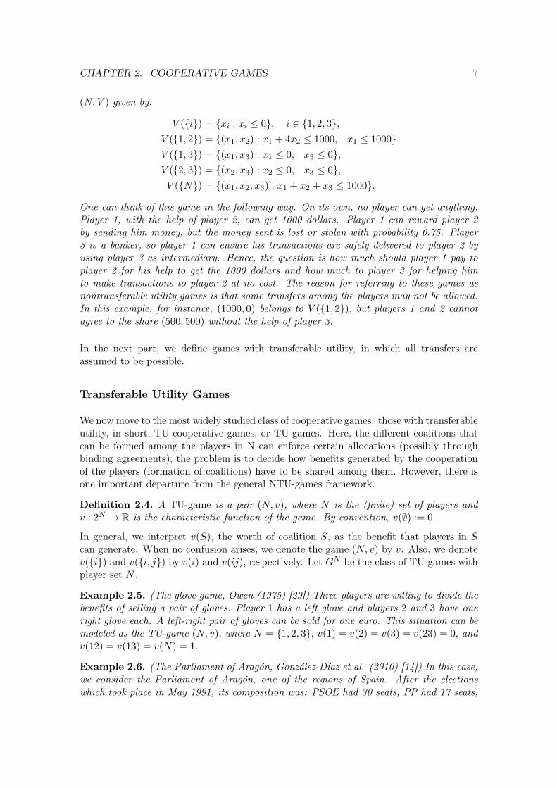
Figure 2.1: The Core of a Cooperative Game with 3 Agents (Example 2.11)
(1, 0, 0)
(0, 1, 0)
(0, 0, 1)
x1 ≤ 1
x3 ≤ 0
x2 ≤ 0
It is easy to see that the only point that meets the constraints is (1, 0, 0) and hence we haveC(w) = {(1, 0, 0)}.
CHAPTER 2. COOPERATIVE GAMES 10
Example 2.12. (Example with 4 agents) Let us consider another cooperative game withfour agents N = {1, 2, 3, 4} and the following characteristic function:
ω({1}) = 0 ω({1, 2}) = 0 ω({1, 2, 3}) = 1 ω({1, 2, 3, 4}) = 2ω({2}) = 0 ω({1, 3}) = 1 ω({1, 2, 4}) = 1ω({3}) = 0 ω({1, 4}) = 1 ω({1, 3, 4}) = 1ω({4}) = 0 ω({2, 3}) = 1 ω({2, 3, 4}) = 1
ω({2, 4}) = 1ω({3, 4}) = 0
Table 2.3: Characteristic Function of a Cooperative Game with 4 Agents
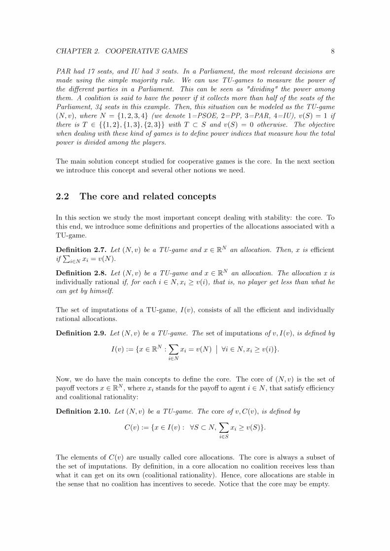
First we will show that the set {(α, α, 1 − α, 1 − α)|α ∈ [0, 1]} is part of the core, i.e.{(α, α, 1− α, 1− α) | α ∈ [0, 1]} ⊆ C(ω). To show it, we just have to prove that (0, 0, 1, 1)and (1, 1, 0, 0) are part of the core. These two payoff distributions are obviously efficientand it is easy to check that they are also coalitionally rational. The core is a convex andcompact polyhedron and hence every linear combination of (0, 0, 1, 1) and (1, 1, 0, 0) is alsopart of the core, i.e.{(α, α, 1− α, 1− α) | α ∈ [0, 1]} ⊆ C(ω).
Now we will prove that C(ω) ⊆ {(α, α, 1 − α, 1 − α) | α ∈ [0, 1]}. A payoff distributionx in the core has to be efficient, thus ω(N) = 2 = x1 + x2 + x3 + x4. It also has to becoalitionally rational hence x1 + x3 ≥ 1, x2 + x4 ≥ 1 and x1 + x4 ≥ 1, x2 + x3 ≥ 1. Ifx1 + x3 > 1 or x2 + x4 > 1, then x1 + x2 + x3 + x4 > 2 = ω(N), therefore x1 + x3 = 1 andx2 + x4 = 1. And if x1 + x4 > 1 or x2 + x3 > 1 then x1 + x2 + x3 + x4 > 2 = ω(N), hencex1 + x4 = 1, x2 + x3 = 1. Since x1 + x3 = 1, x2 + x3 = 1, we can conclude x1 = x2. Sincex1 + x3 = 1 and x1 + x4 = 1, we can conclude x3 = x4. Let x1 = x2 = α then α ≥ 0 sincex1 ≥ 0 = ω({1}). From x1 + x3 = α+ x3 = 1→ x3 = 1− α and x3 ≥ 0 = ω({3}), we seethat α ≤ 1.
Now have proved that C(ω) ⊆ {(α, α, 1 − α, 1 − α) | α ∈ [0, 1]} ⊆ C(ω) hence the core ofour game is C(ω) = {(α, α, 1− α, 1− α) | α ∈ [0, 1]}.
Figure 2.2: The Core of a Cooperative Game with 4 Agents (Example 2.12)
(0, 0, 1, 1)
(0, 0, 0, 2)
(1, 1, 0, 0)
(0, 0, 2, 0)
(2, 0, 0, 0)
(0, 2, 0, 0)
Chapter 3
Assignment problems and linearprogramming
3.1 Assignment problems
Assignment problems deal with the question how to assign n items (e.g. jobs) to nmachines(or workers) in the best possible way. They consist of two components: the assignment asunderlying combinatorial structure and an objective function modeling the “best way”.
Mathematically an assignment is nothing else than a bijective mapping of a finite setinto itself, i.e., a permutation. Assignments can be modeled and visualized in differentways: every permutation Φ of the set N = {1, . . . , n} corresponds in a unique way to apermutation matrix AΦ = (xij) with xij = 1 for j = Φ(i) and xij = 0 for j 6= Φ(i).
We can view this matrix as adjacency matrix of a bipartite graph GΦ = (V,W ;E), wherethe vertex sets V andW have n vertices, i.e., |V | = |W | = n, and there is an edge (i, j) ∈ Eif and only if j = Φ(i).
Pentico (2007) [31] explains the development of what is called “assignment problems” mo-tivated by the 50th aniversary of the seminal paper by Kuhn. This field is a part ofOperations Research, the branch of decision sciences using analytical tools and methods tohelp making better decisions. Usually is devoted to applied problems related to businesses,engineering and organizations. Kuhn’s result allowed a solution of real-world instances,without computers, and the research area is known today as combinatorial optimization.
It is generally recognized that the beginning of the development of practical solution meth-ods for the classic assignment problem was the publication in 1955 of Kuhn’s article on theHungarian method for its solution (Kuhn, 1955) [17]. Naval Research Logistics reprintedit in honor of its 50th anniversary.
There are many different variations corresponding to the assignment problem, and Burkardet al. (2009) [5] is an excellent survey on theoretical methods, algorithms and practicaldevelopments.
Assignment problems involve optimally matching the elements of two or more sets, where
11
CHAPTER 3. ASSIGNMENT PROBLEMS AND LINEAR PROGRAMMING 12
the dimension of the problem refers to the number of sets of elements to be matched. Whenthere are only two sets, they are referred to as “tasks” and “agents”. Thus, for example,“tasks” may be jobs to be done and “agents” the people or machines that can do them, orstudents to be assigned to schools.
The original version of the assignment problem is discussed in almost every textbook foran introductory course in either management science/operations research or productionand operations management. As usually described, the problem is to find a one-to-onematching between n tasks and n agents, the objective being to minimize the total cost ofthe assignments. Classic examples involve such situations as assigning jobs to machines,jobs to workers, or workers to machines.
The linear sum assignment problem (LSAP) is one of the most famous problems in linearprogramming and in combinatorial optimization. Informally speaking, we are given ann× n cost matrix C = (cij) and we want to match each row to a different column in sucha way that the sum of the corresponding entries is minimized. In other words, we want toselect n elements of C so that there is exactly one element in each row and one in eachcolumn and the sum of the corresponding costs is a minimum.
Alternatively, one can define it through a graph theory model. Define a bipartite graphG = (U, V ;E) having a vertex of U for each row, a vertex of V for each column, and costcij associated with edge [i, j] for i, j = 1, 2, . . . , n: The problem is then to determine aminimum cost perfect matching in G (weighted bipartite matching problem: find a subsetof edges such that each vertex belongs to exactly one edge and the sum of the costs ofthese edges is a minimum).
Without loss of generality, we assume that the costs cij are non-negative. Cases withnegative costs can be handled by adding to each element of C a fixed value, the minimumof all entries, ξ. Since we need to select one element per row, any solution of value z for theoriginal cost matrix corresponds to a solution of value z + n × ξ for the transformed costmatrix. In this way we can manage the maximization version of the problem by solvingLSAP on a transformed instance having costs cij = −cij .
We also assume in general that the values in C are finite, with some cij possibly having avery large value (<∞) when assigning i to j is forbidden.
The mathematical expression of the linear sum assignment problem is the following one1:
Minimize z =∑i∈N
∑j∈N
cijxij (3.1)
subject to∑i∈N
xij = 1, for all j ∈ N,∑j∈N
xij = 1, for all i ∈ N,
xij ∈ {0, 1} for all (i, j) ∈ N ×N.
In this dissertation we will use this kind of problems to build a cooperative model usedin economics. The optimal (linear sum) assignment problem is that of finding an optimal
1N:={1,2,. . . ,n}.
CHAPTER 3. ASSIGNMENT PROBLEMS AND LINEAR PROGRAMMING 13
matching, given a matrix that collects the potential profit of each pair of agents. Someexamples are the placement of workers to jobs, of students to colleges, of physicians tohospitals or the pairing of men and women in marriage. Once an optimal matching hasbeen found, one question arises: how to share the output among the partners.
Cooperative games arising from Operations Research have been studied by different authorsand Curiel (1997) [7] or Borm et al. (2001) [4] are good surveys.
3.2 Linear programming
Linear programming is a mathematical technique for solving constrained maximization andminimization problems when there are many constraints and the objective function to beoptimized, as well as the constraints faced, are linear (i.e., can be represented by straightlines).
The subject of linear programming is older than the Second World War. Fourier2 wasamong the first to investigate this subject and point outs its importance to mechanics andprobability theory. The problem that attracted his attention was that of finding a leastmaximum deviation fit to a system of linear equations. He reduced the problem to thatof finding the lowest point of a polyhedron. His suggested solution to this problem can beviewed as a precursor to the modern day simplex algorithm devised by Dantzig3. Dantzigat the time was engaged in a project of an American research program that resulted fromthe intensive scientific activity during the Second World War, aimed at rationalizing thelogistics of the war effort. In the Soviet Union, Kantorovitch4 had already proposed asimilar method for the analysis of economic plans, but his contribution remained unknownto the general scientific community until much later.
The problem of optimizing a linear function subject to linear inequality and equality con-straints is called linear programming (LP). Every linear programming problem can bewritten in the following standard form:
max c · x (3.2)s.t. Ax = b,
x ≥ 0.
Here ’s.t.’ is an abbreviation for ’subject to’. In this standard form, we are given two vectorsb ∈ Rm, c ∈ Rn with a matrix A ∈ Rm×n. In this LP problem, (x1, x2, . . . , xn) ∈ Rn are
2Joseph Fourier (1768-1830) was a French mathematician and physicist best known for initiating theinvestigation of Fourier series and their applications to problems of heat transfer and vibrations. TheFourier transform and Fourier’s law are also named in his honor. Fourier is also generally credited withthe discovery of the greenhouse effect.
3George Bernard Dantzig (November 8, 1914 – May 13, 2005) was an American mathematical scientistwho made important contributions to operations research, computer science, economics, and statistics.Dantzig is known for his development of the simplex algorithm, an algorithm for solving linear programmingproblems.
4Leonid Kantorovitch (1912-1986) was a Soviet mathematician and economist, known for his theory anddevelopment of techniques for the optimal allocation of resources. He is regarded as the founder of linearprogramming. He was the winner of the Stalin Prize in 1949 and the Nobel Memorial Prize in Economicsin 1975.

CHAPTER 3. ASSIGNMENT PROBLEMS AND LINEAR PROGRAMMING 14
the variables that satisfy the constraints which form a polyhedron. This polyhedron iscalled the feasible region of the LP.
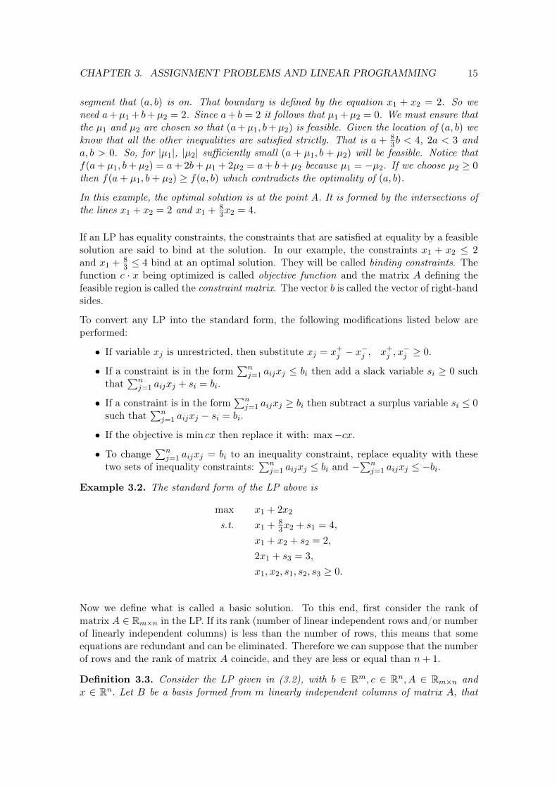
Example 3.1. Here is an example of a Linear Program (LP).
max x1 + 2x2
s.t. x1 + 83 x2 ≤ 4,
x1 + x2 ≤ 2,
2x1 ≤ 3,
x1, x2 ≥ 0.
Figure 3.1: The feasible region of Example 3.1
x2
0 x12x1 = 3 x1 + x2 = 2
B
x1 + 83x2 = 4
A
This polyhedron, the shaded part of Figure 3.1 is called the feasible region of the LP. In thiscase, the feasible region is a polytope. A geometrical rendition of our optimization problemis to find a point in the feasible region that maximizes f(x1, x2) = x1 + 2x2.
Observe that the optimal solution cannot be in the interior of the feasible region.
Suppose it were. Call it (a, b). Let ε ≥ 0 be sufficiently small such that (a + ε, b + ε) isfeasible. Such an ε exists because (a, b) is in the interior of the feasible region. Notice thatf(a+ε, b+ε) = f(a, b)+3ε > f(a, b), contradicting the optimality of (a, b). Therefore thatthe optimal solution must lie on the boundary of the feasible region.
Last remark suggests that one of the extreme points of the feasible region must be an optimalsolution.
Suppose there is an optimal solution on the boundary between the points A and B markedon the figure but not the extreme points A,B. Call it (a, b). Since this point is on theboundary our previous argument does not apply because (a+ ε, b+ ε) need not be feasible.The idea is to perturb (a, b) to a new feasible point that is still on the same boundarysegment. Consider the point (a + µ1, b + µ2). We want this to be on the same boundary
CHAPTER 3. ASSIGNMENT PROBLEMS AND LINEAR PROGRAMMING 15
segment that (a, b) is on. That boundary is defined by the equation x1 + x2 = 2. So weneed a+µ1 + b+µ2 = 2. Since a+ b = 2 it follows that µ1 +µ2 = 0. We must ensure thatthe µ1 and µ2 are chosen so that (a+µ1, b+µ2) is feasible. Given the location of (a, b) weknow that all the other inequalities are satisfied strictly. That is a + 8
3b < 4, 2a < 3 anda, b > 0. So, for |µ1|, |µ2| sufficiently small (a + µ1, b + µ2) will be feasible. Notice thatf(a+ µ1, b+ µ2) = a+ 2b+ µ1 + 2µ2 = a+ b+ µ2 because µ1 = −µ2. If we choose µ2 ≥ 0then f(a+ µ1, b+ µ2) ≥ f(a, b) which contradicts the optimality of (a, b).
In this example, the optimal solution is at the point A. It is formed by the intersections ofthe lines x1 + x2 = 2 and x1 + 8
3x2 = 4.
If an LP has equality constraints, the constraints that are satisfied at equality by a feasiblesolution are said to bind at the solution. In our example, the constraints x1 + x2 ≤ 2and x1 + 8
3 ≤ 4 bind at an optimal solution. They will be called binding constraints. Thefunction c · x being optimized is called objective function and the matrix A defining thefeasible region is called the constraint matrix. The vector b is called the vector of right-handsides.
To convert any LP into the standard form, the following modifications listed below areperformed:
• If variable xj is unrestricted, then substitute xj = x+j − x
−j , x+
j , x−j ≥ 0.
• If a constraint is in the form∑n
j=1 aijxj ≤ bi then add a slack variable si ≥ 0 suchthat
∑nj=1 aijxj + si = bi.
• If a constraint is in the form∑n
j=1 aijxj ≥ bi then subtract a surplus variable si ≤ 0such that
∑nj=1 aijxj − si = bi.
• If the objective is min cx then replace it with: max−cx.
• To change∑n
j=1 aijxj = bi to an inequality constraint, replace equality with thesetwo sets of inequality constraints:
∑nj=1 aijxj ≤ bi and −
∑nj=1 aijxj ≤ −bi.
Example 3.2. The standard form of the LP above is
max x1 + 2x2
s.t. x1 + 83x2 + s1 = 4,
x1 + x2 + s2 = 2,
2x1 + s3 = 3,
x1, x2, s1, s2, s3 ≥ 0.
Now we define what is called a basic solution. To this end, first consider the rank ofmatrix A ∈ Rm×n in the LP. If its rank (number of linear independent rows and/or numberof linearly independent columns) is less than the number of rows, this means that someequations are redundant and can be eliminated. Therefore we can suppose that the numberof rows and the rank of matrix A coincide, and they are less or equal than n+ 1.
Definition 3.3. Consider the LP given in (3.2), with b ∈ Rm, c ∈ Rn, A ∈ Rm×n andx ∈ Rn. Let B be a basis formed from m linearly independent columns of matrix A, that
CHAPTER 3. ASSIGNMENT PROBLEMS AND LINEAR PROGRAMMING 16
is the corresponding submatrix. Choose x ∈ Rn so as for xj such that j ∈ B is to solveBxB = b, and xj = 0 if j /∈ B. The resulting solution is called a basic solution.
Notice the choice will be unique because B is a non-singular square matrix.
If a basic solution x associated with the basis B, x = [xB|0] = [B−1b|0], is non-negativethen x is a basic feasible solution to the LP.
Example 3.4. Consider the LP
x1 + x2 + x3 = 1,2x1 + 3x2 = 1,x1, x2, x3 ≥ 0.
The constraint matrix is (1 1 12 3 0
),
and here is one basis: (1 12 0
).
To find the basic solution associated with this basis, we set x2 = 0 and solve
x1 + x3 = 1,2x1 + 0x3 = 1.
So, the basic solution is x1 = 12 , x2 = 0 and x3 = 1
2 , which also happens to be a basicfeasible solution.
Another basis is (1 12 3
),
The basic solution associated with this basis is found by setting x3 = 0 and solving
x1 + x2 = 1,2x1 + 3x2 = 1.
The basic solution is x1 = 2, x2 = −1 and x3 = 0 which is not a basic feasible solution.
Now we prove that the solution of the LP is found in an extreme point if the program isfeasible.
Lemma 3.5. Consider the LP given in (3.2), with b ∈ Rm, c ∈ Rn, A ∈ Rm×n and x ∈ Rn.If the set {x ∈ Rn : Ax = b, x ≥ 0} is feasible, then it has a basic feasible solution.
Proof. Let x′ ∈ Rn be a feasible solution. Then x′j ≥ 0, j ∈ {1, 2, . . . , n} and∑
j∈S aijx′j =
bi, for i ∈ {1, 2, . . . ,m} where A = (aij). We can ignore terms such that x′j = 0 and takeS = {j ∈ {1, . . . , n} : x′j 6= 0}. Let {aj} be the columns of matrix A, for j ∈ {1, . . . , n}.If the set {aj : j ∈ S} are linearly independent we are done: if the cardinality of this set
CHAPTER 3. ASSIGNMENT PROBLEMS AND LINEAR PROGRAMMING 17
is less than m, throw in some additional columns of the A matrix to produce a set of mlinearly independent vectors. The variables associated with these extra columns take thevalue zero. Then x′ is a basic feasible solution.
Assume {aj : j ∈ S} are not linearly independent. Then there exists {λj} not all zero s.t.∑j∈S λja
j = 0. Let x′′ = x′ − θλ ≥ 0 by picking θ as small as necessary. The columns ofA associated with the positive components of x′′ involve one fewer independent column.Next, we verify that x′′ is feasible.
Ax′′ = A(x′ − θλ) = Ax′ − θAλ = Ax′ − θ∑j∈S
λj ∗ aj = Ax′ − θ ∗ 0 = Ax′ = b
If the columns associated with the non-zero components of x′′ are linearly dependent, repeatthe argument above. As there are finite number of columns and the method eliminates onecolumn at each iteration, it will terminate after a finite number of steps.
Lemma 3.6. Consider the LP given in (3.2), with b ∈ Rm, c ∈ Rn, A ∈ Rm×n and x ∈ Rn.If x∗ is a basic feasible solution of the set {x : Ax = b, x ≥ 0}, then x∗ is an extreme pointof the set.
Proof. If x* is not an extreme point there exist feasible y and z, distinct from x*, such thatx* = λy+ (1− λ)z. Let B the basis associated with x* and set x* = [xB|xN ], A = [B|N ],y = [yB|yN ], z = [zB|zN ], where N is the rest of the columns. From the definitions wehave λyN + (1− λ)zN = xN = 0⇒ yN = zN = 0 = xN .
Feasibility impliesAy = b⇒ ByB = b
andAz = b⇒ BzB = b,
but xB is the unique solution to Bx = b. Then xB = zB = yB, so x*= z = y. As a resultthere do not exist z, y different than x∗. Therefore x∗ is an extreme point.
Theorem 3.7. Consider the LP given in (3.2), with b ∈ Rm, c ∈ Rn, A ∈ Rm×n andx ∈ Rn and let P = {x ∈ Rn : Ax = b, x ≥ 0}. If A is of full row rank and maxx∈P cx hasa finite optimal solution, there is an optimal solution at one of the extreme points of P .
Proof. In order to prove this theorem, Lemma 3.5 can be used. The reader is referred toVohra (2005) [40] for its complete proof.
Associated with each LP is another LP called its dual. The original LP is called the primal.
Upper bounds on the optimal objective function value can be found by taking appropriatelinear combinations of constraints (yA) that dominate the objective function c, i.e., c ≤yA⇒ cx ≤ yAx since x ≥ 0. Using the fact that Ax = b allows one to conclude that
CHAPTER 3. ASSIGNMENT PROBLEMS AND LINEAR PROGRAMMING 18
cx ≤ yAx = yb⇒ cx ≤ yb
Thus yb is an upper bound on the objective function value.
Definition 3.8. The dual is the problem of finding the smallest function value such upperbound from the primal LP.
Primal(P)
Zp = max cxs.t. Ax = b
x ≥ 0
=⇒
Dual(D)
Zp = min ybs.t. yA ≥ c
y unrestricted.
Example 3.9 (Example 3.2 continued). We derive the dual to the Example 3.2 above.
max x1 + 2x2
s.t. x1 + 83x2 + s1 = 4,
x1 + x2 + s2 = 2,
2x1 + s3 = 3,
x1, x2, s1, s2, s3 ≥ 0.
The dual of the example problem will be
min 4y1 + 2y2 + 3y3
s.t. y1 + y2 + 2y3 ≥ 1,83y1 + y2 ≥ 2,
y1, y2, y3 ≥ 0.
Now we introduce Farkas’ Lemma. It is used for our LP problem and it can also be usedin the proof of the Karush-Kuhn-Tucker Theorem. It simply says that a vector is either ina convex cone or there is an hyperplane separating the vector from the cone (separatinghyperplane).
Lemma 3.10. (Farkas’ 5 Lemma) Let A be an m×n matrix, b ∈ Rm, and F = {x ∈ Rn :Ax = b, x ≥ 0}. Then either F 6= ∅ or there exists y ∈ Rm such that yA ≥ 0 and yb < 0but not both.
Proof. The proof of Farkas’ Lemma can be found in several books under different forms.The reader is referred to Vohra (2005) [40].
Lemma 3.11. If problem (P) is infeasible then (D) is either infeasible or unbounded. If(D) is unbounded then (P) is infeasible.
5Farkas Gyula, or Julius Farkas (1847–1930) was a Hungarian mathematician and physicist. TheHungarian Academy of Science elected him corresponding member May 6, 1898. He has made contributionto linear algebra with Farkas’ lemma, which is named after him for his derivation of it.
CHAPTER 3. ASSIGNMENT PROBLEMS AND LINEAR PROGRAMMING 19
Proof. Suppose for a contradiction that (D) has a finite optimal solution, y∗, say. Infea-sibility of (P) implies by Lemma 3.10 (Farkas’ Lemma) that there exists a vector y suchthat yA ≥ 0 and y · b < 0. Let t > 0. The vector y∗ + ty is a feasible solution for (D)since (y∗ + ty)A ≥ y∗A ≥ c. Its objective function value is (y∗ + ty) · b < y∗b, contradict-ing the optimality of y∗. Since (D) cannot have a finite optimal, it must be infeasible orunbounded.
Now suppose (D) is unbounded. Because of the feasible set is a polyhedron, we can writeany solution of (D) as y + r where y is a feasible solution to the dual and r is a ray, i.e.,yA ≥ c and rA ≥ 0. Furthermore r·b < 0 since (D) is unbounded. By Farkas’ Lemma, theexistence of r implies the primal is infeasible.
Theorem 3.12. (Duality theorem) Let ZP , ZD be the sets of optimal solutions for (P)and (D) respectively. If a finite optimal solution for either the primal or dual exists, thenZP = ZD.
Proof. The reader can find two proofs of this theorem in Vohra (2005) [40].


Chapter 4
Assignment games
The aim of this chapter is to present formally the assignment market, focusing on theassociated cooperative game, introduced by Shapley and Shubik (1971). The assignmentproblem has been analyzed in operations research long before the assignment game wasinvestigated.
The assignment game is a model for a two-sided market in which a product that comesin indivisible units (e.g., houses, cars, etc.) is exchanged for money, and in which eachparticipant either supplies or demands exactly one unit. The units need not be alike, andthe same unit may have different values to different participants.
4.1 The assignment model
An assignment game is a model for a two-sided market introduced by Shapley1 and Shubik2
(1971). There are two disjoint sets of agents, let us call them buyers and sellers and denotethem by M and M ′ respectively. In this market, there are m buyers and m′ sellers.Therefore, the assignment market is integrated by a finite set of agents M of cardinality|M | = m which has to be assigned to a set of tasks M ′ of cardinality |M ′| = m′. Eachbuyer i ∈ M is willing to buy at most one good and each seller j ∈ M ′ has exactly onegood on sale. Assume hij ≥ 0 is how much buyer i ∈ M values the good of seller j ∈ M ′and cj ≥ 0 is the reservation value of this seller, meaning j will not sell his good for a lowerprice. Then, whenever hij ≥ cj , there is room too agree on some price hij ≥ p ≥ cj and thejoint profit of this trade is (hij − p) + (p− cj). As a consequence, we consider a valuationmatrix A = (aij)(i,j)∈M×M ′ that represents the joint profit obtained by a mixed-pair of abuyer and a seller that is aij = max{hij − cj , 0} ∀i ∈M,∀j ∈M ′.
Formally, we denote this market by γ = (M,M ′;A).1Lloyd Stowell Shapley (June 2, 1923 - March 12, 2016) was a distinguished American mathematician
and Nobel Prize winning economist (2012). He was a Professor Emeritus at University of California, LosAngeles (UCLA), affiliated with departments of Mathematics and Economics. He contributed to the fieldsof mathematical economics and especially game theory.
2Martin Shubik (born March 24, 1926) is an American economist, who is Professor Emeritus of Math-ematical Institutional Economics at Yale University. Shubik specializes in strategic analysis, the study offinancial institutions, the economics of corporate competition, and game theory.
21

CHAPTER 4. ASSIGNMENT GAMES 22
4.2 The assignment game
Shapley and Shubik (1971) [36] associates to each assignment market (M,M ′, A) a coop-erative game which is called the assignment game.
Definition 4.1. Let γ = (M,M ′;A) be an assignment market. The associated assignmentgame (M ∪M ′, ωA) is defined by a set of agents (the union of buyers and sellers: M ∪M ′)and the characteristic function ωA which associates to each coalition of agents the maximumbenefit they can get by assigning buyers and sellers inside this coalition.
Definition 4.2. Let γ = (M,M ′;A) be an assignment market. A matching µ between Mand M ′ is a subset of the cartesian product, M ×M ′, such that each agent belongs to atmost one pair.
We denote byM(M,M ′) the set of all possible matchings.
Definition 4.3. A matching µ ∈ M(M,M ′) is optimal for the market (M,M ′;A) if∑(i,j)∈µ
aij ≥∑
(i,j)∈µ′aij for all µ′ ∈M(M,M ′).
The set of all optimal matchings for the market (M,M ′;A) is denoted byMA(M,M ′). Anoptimal matching µ can be found by solving the so-called linear assignment problem.
Definition 4.4. Let γ = (M,M ′;A) be an assignment market and (M ∪ M ′, ωA) itsassociated assignment game. The value for the total coalition ωA(M ∪M ′) is the optimumvalue of the linear program:
max z =∑i∈M
∑j∈M ′
aijµij (4.1)
s.t.∑i∈M
µij ≤ 1, for all j ∈M ′,∑j∈M ′
µij ≤ 1, for all i ∈M,
µij ∈ {0, 1} for all (i, j) ∈M ×M ′.
Notice that this is an integer linear program, and by the definition of the linear program,matrix (µij)(i,j)∈M×M ′ has at most only one non-zero entry for each row and column. Ifµ ∈ {0, 1}M×M ′ is a solution of (4.1), then µ = {(i, j) | µij = 1} is an optimal matching.
We now consider the continuous relaxation, or continuous case of this integer linear pro-gram. This is our next linear program (4.2) and we will solve it using several well knownalgorithms. Notice that matrices (µij)(i,j)∈M×M ′ which are solutions of our first programare also solutions of the continuous relaxation program:
CHAPTER 4. ASSIGNMENT GAMES 23
max z =∑i∈M
∑j∈M ′
aijµij (4.2)
s.t.∑i∈M
µij ≤ 1, for all j ∈M ′,∑j∈M ′
µij ≤ 1, for all i ∈M,
µij ≥ 0 for all (i, j) ∈M ×M ′.
One of most well-known solutions of the assignment problem, the Hungarian method, wasprovided by Harold Kuhn 3 [17] in 1955, even though Carl Gustav Jacobi already discoveredthe same solution in the 19th century4.
In fact, the assignment problem is a special case of the transportation problem. Othersolutions e.g. the simplex method provided by Dantzig (1963) [8] can also be used to findan optimal matrix that maximizes z. The solution of the assignment problem (see Dantzig(1963), p. 318) shows that the optimal value for 4.2 is attained with all µij ∈ {0, 1}, forall (i, j) ∈M ×M ′ . This result was independently proved in Birkhoff5 (1946) [2] and vonNeumann6 (1953) [43]. Hence this implies a solution to the assignment problem 4.1.
Since the solution of the assignment problem deals with a linear program, it allows us toconsider the linear program that is dual to the first program (4.2):
min z =∑i∈M
ui +∑j∈M ′
vj (4.3)
s.t. ui + vj ≥ aij for all (i, j) ∈M ×M ′,ui ≥ 0, for all i ∈M,
uj ≥ 0, for all j ∈M ′.
Therefore, because of the Duality Theorem (Theorem 3.12) for linear programming, wecan state the following corollary.
Corollary 4.5. The solution of the dual program (4.3) coincides with the solution of thelinear program (4.1).
3Harold William Kuhn (July 29, 1925 – July 2, 2014) was an American mathematician known for theKarush–Kuhn–Tucker conditions, for Kuhn’s theorem, for developing Kuhn poker as well as the descriptionof the Hungarian method for the assignment problem.
4Jacobi’s solution was rediscovered in 2006. Further information can be found in Cariñena, J. et al.(2006) [6].
5George David Birkhoff (March 21, 1884 – November 12, 1944) was an American mathematician, bestknown for what is now called the ergodic theorem. He introduced the chromatic polynomiale and provedPoincaré’s "Last Geometric Theorem," a special case of the three-body problem.
6John von Neumann (December 28, 1903 – February 8, 1957) was a Hungarian-American pure andapplied mathematician, physicist, inventor, computer scientist, and polymath. He was a pioneer of theapplication of operator theory to quantum mechanics, in the development of functional analysis, and a keyfigure in the development of game theory.
CHAPTER 4. ASSIGNMENT GAMES 24
To finish the description of the game, now we can define the characteristic function. Recallthat N = M ∪ M ′, The characteristic function ωA(S) defines the benefit that can beobtained by each coalition.
Definition 4.6. Let γ = (M,M ′;A) be an assignment market and (M ∪ M ′, ωA) itsassociated assignment game. The characteristic function ωA(S) defines the benefit that canbe obtained by each coalition and it is expressed in the following form
ωA(S) = maxµ∈M(M∩S,M ′∩S)
∑(i,j)∈µ
aij for all S ⊆ N.
Notice that ωA(S) is the optimal value of the linear program (4.1) restricted to i ∈ S ∩Mand j ∈ S ∩M ′.
The concept of solution more studied for cooperative games in general, and for the assign-ment games in particular, is the core.
CHAPTER 4. ASSIGNMENT GAMES 25
4.3 The core of the assignment game
Definition 4.7. Given an assignment game (M ∪M ′, ωA), an imputation is a vector ofpayments (u, v) ∈ Rm+ × Rm
′+ where ui ≥ 0 is the payment to buyer i ∈ M and vj ≥ 0 is
the payment to seller j ∈M ′, such that∑i∈M
ui +∑j∈M ′
vj = ωA(M ∪M ′).
We denote I(ωA) the set of imputations of the assignment game.
Now we define the core of the assignment game.
Definition 4.8. The core of an assignment game (M ∪M ′, ωA) is the set of those impu-tations such that every coalition receives, at least, its value according to the characteristicfunction:
C(ωA) =
(u, v) ∈ I(ωA)
∣∣∣∣ ∑i∈S∩M
ui +∑
j∈S∩M ′vj ≥ ωA(S) ∀S ⊆M ∪M ′
.
Theorem 4.9. (Shapley and Shubik, 1971 [36]) Let γ = (M,M ′;A) be an assignment mar-ket. Then, its corresponding assignment game (N,ωA) has a non-empty core. Moreover,the core coincides with the set of dual solutions to the linear assignment problem.
Proof. Consider the assignment market γ = (M,M ′;A) and its corresponding game (N,ωA).An optimal matching µ can be found by solving the so-called linear assignment problem:
max∑i∈M
∑j∈M ′
aijxij (4.4)
s.t.∑i∈M
xij ≤ 1, for all j ∈M ′,∑j∈M ′
xij ≤ 1, for all i ∈M,
xij ∈ {0, 1} for all (i, j) ∈M ×M ′.
By the Birkhoff-von Neumann Theorem the solution of the above integer linear programcoincides with its LP relaxation, which is the related continuous linear program withxij ≥ 0 for all (i, j) ∈M ×M ′. The fundamental duality theorem states that every linearprogram can be transposed into a dual form and, if the primal program has a solution,then the optimal values of both programs coincide. Then, the dual of the LP relaxation ofthe primal program (4.4) is:
min∑i∈M
ui +∑j∈M ′
vj (4.5)
s.t. ui + vj ≥ aij for all (i, j) ∈M ×M ′,ui ≥ 0 for all i ∈M,
vj ≥ 0 for all j ∈M ′.
CHAPTER 4. ASSIGNMENT GAMES 26
In our case, the fundamental duality theorem tells that (4.5) has a solution and, over therespective sets of constraints, min
∑i∈M
ui +∑j∈M ′
vj = max∑i∈M
∑j∈M ′
aijxij = ωA(M ∪M ′).
Hence, a payoff vector (u, v) is a solution of the dual program (4.5) if and only if it is anelement of the core of (N,ωA). As a consequence, the core is non-empty.
Shapley and Shubik (1971) [36] shows that it is sufficient to take into account mixed-paircoalitions to describe the core. Then, for each optimal matching µ ∈MA(M,M ′), the coreof the corresponding assignment game (N,ωA) is described by
C(ωA) =
{(u, v) ∈ RM+ × RM
′+
∣∣∣∣ ui + vj = aij for all (i, j) ∈ µ andui + vj ≥ aij for all (i, j) ∈M ×M ′
}.
By the nature of the assignment game, the core only considers ui, uj ≥ 0 for all i ∈M, j ∈M ′ where ui = 0 if i is unmatched by µ and vj = 0 if j unmatched by µ.
Shapley and Shubik prove that the core of an assignment game is always non-empty, thatis, assignment games are balanced7.
The set of dual solutions of the assignment problem had already been analyzed by Gale(1960) [11] and related to his notion of competitive equilibrium. As in Roth and Sotomayor(1990) [33], let us assume that M ′ contains as many copies as necessary of a null objecto ∈ O such that aiO = 0 for all i ∈ M . Then, for any matching µ, all buyers can beassumed to be matched either to a real object or to a null object O.
Definition 4.10 (Gale, 1960 [11]). Given a vector of non-negative prices p ∈ RM ′, withpO = 0, the demand set of buyer i ∈M at prices p is
Dp(i) = {j ∈M ′ | aij − pj = maxk∈M ′
{aik − pk}}.
This means that buyer i asks for those objects that give him the maximum profit, givenby the difference of valuation and price.
Then, a pair (p, µ) formed by a vector of prices and a matching is a competitive equilibriumif µ(i) ∈ Di(p) for all i ∈ M and pj = 0 whenever j ∈ M ′ is unassigned by µ. In thiscase, p is said to be a competitive equilibrium price vector. Given a competitive equilibrium(p, µ), the payoff vector (u, v) where ui = aiµ(i) − pµ(i) for all i ∈ M and vj = pj for allj ∈M ′ is a competitive equilibrium payoff vector.
Theorem 4.11 (Gale, 1960 [11]). For any assignment game, the set of solutions of thedual program of (4.1) coincides with the set of competitive equilibrium payoff vectors.
Proof. Given a solution (u, v) of the dual program, define p = v ∈ RM ′+ . Take µ an optimalmatching. From
∑(i,j)∈µ
aij =∑i∈M
ui +∑j∈M ′
vj and ui + vj ≥ aij for all (i, j) ∈ µ it follows
that pj = vj = 0 for all unassigned object j ∈M ′ and ui + vj = aij if (i, j) ∈ µ. Moreover,for all i ∈M ,
aiµ(i) − pµ(i) = ui ≥ aij − pj for all j ∈M ′,7A game (N, v) is said to be balanced if it has a non-empty core.
CHAPTER 4. ASSIGNMENT GAMES 27
where the inequality follows from the dual program constraints. Hence, p is a competitiveprice vector.
Conversely, if p is a competitive price vector, then there exists µ ∈ M(M,M ′) such thatpj = 0 if j is unassigned by µ and for all i ∈M ,
µ(i) ∈ Di(p).
Define now (u, v) ∈ RM × RM ′ by vj = pj for all j ∈ M ′ and ui = aiµ(i) − pµ(i) for alli ∈ M . Notice that if i ∈ M is assigned to a null object, then ui = 0. Also, vj = 0 ifj /∈ µ(M). Let us check that (u, v) is a solution of the dual problem.
We see first that if (p, µ) is a competitive equilibrium, then µ is an optimal matching.Indeed, take another matching µ′ ∈ M(M,M ′). Now, since aiµ(i) − pµ(i) ≥ aiµ′(i) − pµ′(i)for all i ∈M ,∑
(i,j)∈µ
aij =∑i∈M
aiµ(i) ≥∑i∈M
(aiµ′(i) − pµ′(i)) +∑i∈M
pµ(i)
=∑i∈M
aiµ′(i) −∑
j∈µ′(M)
pj +∑
j∈µ(M)
pj
=∑i∈M
aiµ′(i) −∑
j∈µ′(M)\µ(M)
pj +∑
j∈µ(M)\µ′(M)
pj
≥∑i∈M
aiµ′(i)
where the last inequality follows from the fact that (p, µ) is a competitive equilibrium andhence pj = 0 for all j /∈ µ(M).
Since µ is an optimal matching and agents assigned to the null object receive zero,
ωA(M ∪M ′) =∑i∈M
aiµ(i) =∑i∈M
ui + vµ(i) =∑i∈M
ui +∑j∈M ′
vj ,
which means (u, v) is efficient.
Finally, for all i ∈M and for all j ∈M ′,
ui + vj = ui + pj = aiµ(i) − pµ(i) + pj
≥ aij − pj + pj = aij ,
which concludes the proof that (u, v) is a solution of the dual program.
Theorem 4.12. Let γ = (M,M ′;A) be an assignment market and (M ∪ M ′, ωA) itsassociated assignment game. For the assignment game, the four sets below coincide:
• The core, C(wA).
• The set of dual solutions to the assignment problem (4.1).
• The set of competitive equilibrium payoff vectors of the market.
CHAPTER 4. ASSIGNMENT GAMES 28
• The set of pairwise-stable payoff vectors.
Now we put several examples of an assignment game and its core.
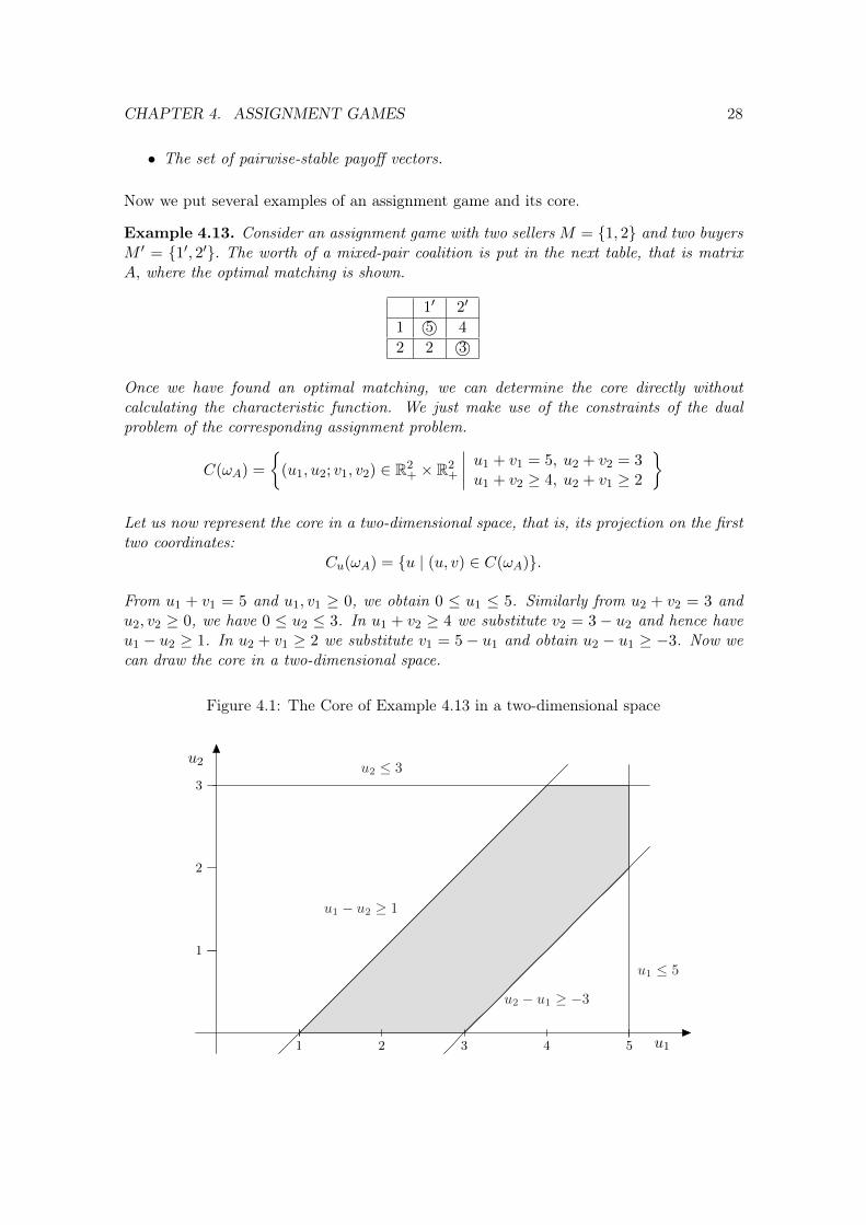
Example 4.13. Consider an assignment game with two sellers M = {1, 2} and two buyersM ′ = {1′, 2′}. The worth of a mixed-pair coalition is put in the next table, that is matrixA, where the optimal matching is shown.
1′ 2′
1 5© 4
2 2 3©
Once we have found an optimal matching, we can determine the core directly withoutcalculating the characteristic function. We just make use of the constraints of the dualproblem of the corresponding assignment problem.
C(ωA) =
{(u1, u2; v1, v2) ∈ R2
+ × R2+
∣∣∣∣ u1 + v1 = 5, u2 + v2 = 3u1 + v2 ≥ 4, u2 + v1 ≥ 2
}
Let us now represent the core in a two-dimensional space, that is, its projection on the firsttwo coordinates:
Cu(ωA) = {u | (u, v) ∈ C(ωA)}.
From u1 + v1 = 5 and u1, v1 ≥ 0, we obtain 0 ≤ u1 ≤ 5. Similarly from u2 + v2 = 3 andu2, v2 ≥ 0, we have 0 ≤ u2 ≤ 3. In u1 + v2 ≥ 4 we substitute v2 = 3− u2 and hence haveu1 − u2 ≥ 1. In u2 + v1 ≥ 2 we substitute v1 = 5− u1 and obtain u2 − u1 ≥ −3. Now wecan draw the core in a two-dimensional space.
Figure 4.1: The Core of Example 4.13 in a two-dimensional space
1 2 3 4 5
u2
u1
1
2
3
u2 − u1 ≥ −3
u1 − u2 ≥ 1
u1 ≤ 5
u2 ≤ 3
CHAPTER 4. ASSIGNMENT GAMES 29
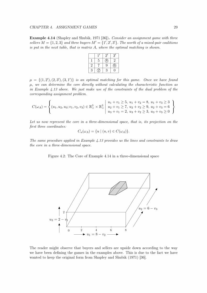
Example 4.14 (Shapley and Shubik, 1971 [36]). Consider an assignment game with threesellersM = {1, 2, 3} and three buyersM ′ = {1′, 2′, 3′}. The worth of a mixed-pair coalitionsis put in the next table, that is matrix A, where the optimal matching is shown.
1′ 2′ 3′
1 5 8© 2
2 7 9 6©3 2© 3 0
µ = {(1, 2′), (2, 3′), (3, 1′)} is an optimal matching for this game. Once we have foundµ, we can determine the core directly without calculating the characteristic function asin Example 4.13 above. We just make use of the constraints of the dual problem of thecorresponding assignment problem.
C(ωA) =
(u1, u2, u3; v1, v2, v3) ∈ R3+ × R3
+
∣∣∣∣∣∣u1 + v1 ≥ 5, u1 + v2 = 8, u1 + v3 ≥ 3u2 + v1 ≥ 7, u2 + v2 ≥ 9, u2 + v3 = 6u3 + v1 = 2, u3 + v2 ≥ 3, u3 + v3 ≥ 0
Let us now represent the core in a three-dimensional space, that is, its projection on thefirst three coordinates:
Cu(ωA) = {u | (u, v) ∈ C(ωA)}.
The same procedure applied in Example 4.13 provides us the lines and constraints to drawthe core in a three-dimensional space.
Figure 4.2: The Core of Example 4.14 in a three-dimensional space
2 4 6 8
2
0u1 = 8− v2
u3 = 2− v1
u2 = 6− v3
The reader might observe that buyers and sellers are upside down according to the waywe have been defining the games in the examples above. This is due to the fact we havewanted to keep the original form from Shapley and Shubik (1971) [36].
CHAPTER 4. ASSIGNMENT GAMES 30
Notice that some examples seen as cooperative games from Chapter 2 are actually assign-ment games. Let us show them down below.
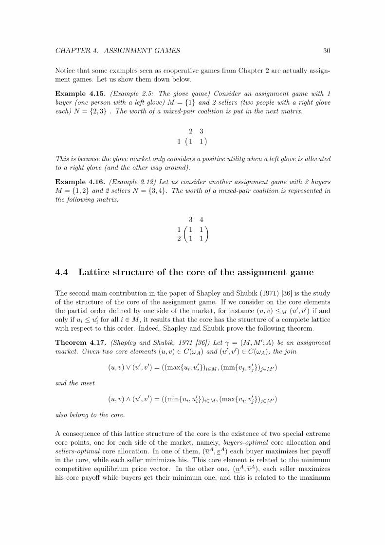
Example 4.15. (Example 2.5: The glove game) Consider an assignment game with 1buyer (one person with a left glove) M = {1} and 2 sellers (two people with a right gloveeach) N = {2, 3} . The worth of a mixed-pair coalition is put in the next matrix.
( 2 3
1 1 1)
This is because the glove market only considers a positive utility when a left glove is allocatedto a right glove (and the other way around).
Example 4.16. (Example 2.12) Let us consider another assignment game with 2 buyersM = {1, 2} and 2 sellers N = {3, 4}. The worth of a mixed-pair coalition is represented inthe following matrix.
( 3 4
1 1 12 1 1
)
4.4 Lattice structure of the core of the assignment game
The second main contribution in the paper of Shapley and Shubik (1971) [36] is the studyof the structure of the core of the assignment game. If we consider on the core elementsthe partial order defined by one side of the market, for instance (u, v) ≤M (u′, v′) if andonly if ui ≤ u′i for all i ∈M , it results that the core has the structure of a complete latticewith respect to this order. Indeed, Shapley and Shubik prove the following theorem.
Theorem 4.17. (Shapley and Shubik, 1971 [36]) Let γ = (M,M ′;A) be an assignmentmarket. Given two core elements (u, v) ∈ C(ωA) and (u′, v′) ∈ C(ωA), the join
(u, v) ∨ (u′, v′) = ((max{ui, u′i})i∈M , (min{vj , v′j})j∈M ′)
and the meet
(u, v) ∧ (u′, v′) = ((min{ui, u′i})i∈M , (max{vj , v′j})j∈M ′)
also belong to the core.
A consequence of this lattice structure of the core is the existence of two special extremecore points, one for each side of the market, namely, buyers-optimal core allocation andsellers-optimal core allocation. In one of them, (uA, vA) each buyer maximizes her payoffin the core, while each seller minimizes his. This core element is related to the minimumcompetitive equilibrium price vector. In the other one, (uA, vA), each seller maximizeshis core payoff while buyers get their minimum one, and this is related to the maximum
CHAPTER 4. ASSIGNMENT GAMES 31
competitive equilibrium price vector. Moreover, these are the two more distant pointsinside the core. What is remarkable is that all agents on the same side of the market,despite being competing for the best deal, obtain their maximum core payoff in the samecore element.
Theorem 4.18. (Shapley and Shubik, 1971 [36]) Let γ = (M,M ′;A) be an assignmentmarket. The core of the assignment game C(ωA) always contains a buyer and a selleroptimum.
Proof. The basic idea behind the proof is related to the special form of the restrictions ofthe core, where each variable has 1 as a coefficient. Figure of Example 4.13 might helpvisualizing this idea. We will show that for any allocations (u′, v′) and (u′′, v′′) that arepart of the core the allocations (
˜u, v) and (u,
˜v) with
˜ui = min{u′i, u′′i } i ∈M,
˜vj = min{v′j , v′′j } j ∈M ′,ui = max{u′i, u′′i } i ∈M,
vj = max{v′j , v′′j } j ∈M ′.
are themselves in the core. This is equivalent to say that the core points form a lattice(Birkhoff, 1973) [3]. We first prove that (
˜u, v) is coalitionally rational. For all i ∈ M ,
j ∈M ′, we have
˜ui + vj = min{u′i + vj , u
′′i + vj}
≥ min{u′i + v′j , u′′i + v′′j }
≥ aij .
Now we have to show that (˜u, v) is an imputation. Let µ be an optimal assignment, then
we have
˜ui = min{u′i, u′′i }
= min{aiµ(i) − v′µ(i), aiµ(i) − v′′µ(i)}= aiµ(i) −max{v′µ(i), v
′′µ(i)}
= aiµ(i) − vµ(i).
For any player that is not assigned we have˜ui = 0 and vj = 0, and hence∑
i∈M ˜ui +
∑j∈M ′
vj =∑i∈M
aiµ(i) = w(M ∪M ′).
Similarly (˜u, v) ∈ C(ωA).
Let us consider ui = min(u,v)∈C(ωA){ui} for all i ∈ M and ui = max(u,v)∈C(ωA){ui} for alli ∈ M . In the same way we define vj and vj . Since the core is compact (for any generalcooperative game), there exists a vector that contains the minimum uk and another vectorwhich contains the minimum ul. With these two vectors we can construct a new vector,using the lattice structure, which contains uk and ul and is also part of the core. If
CHAPTER 4. ASSIGNMENT GAMES 32
we continue this process we obtain a core allocation (u, v) where all sellers receive thereminimum payoff. We know that in the core each optimal pair (i, µ∗(i)) receives aiµ∗(i) ,i.e. ui + vµ∗(i) = aiµ∗(i). So if ui is minimum vµ∗(i) is maximum, i.e. vµ∗(i) = aiµ∗(i) − ui.Therefore we have (u, v) = (u, v). In the same way we can show that (u, v) is part of thecore, too.
It is quite obvious that there are no other core allocations which are further away from eachother than (u, v) and (u, v) since for any core elements (u′, v′) and (u′′, v′′) the followinginequalities hold true:
|ui − ui| ≥ |u′i − u′′i | ∀i ∈M ,|vj − vj | ≥ |v′j − v′′j | ∀j ∈M ′.
We have proved that the core is a lattice with a maximum and a minimum. Since thetotal payoff of any core vector is always the same, a maximum in this context refers to amaximum payoff for all buyers or all sellers. If the payoff for all buyers is maximum, thepayoff for sellers is also determined and minimum.
Roth and Sotomayor (1990) [33] provides a neat proof of a result presented, independently,in Demange [9] (1982) and Leonard [18] (1983). It says that the maximum core payoff ofan agent, be it a buyer or a seller, is her/his marginal contribution to the grand coalition.That is the following lemma.
Lemma 4.19. Given an assignment game (M ∪M ′, wA), the maximum core payoff of anagent is his/her marginal contribution to the grand coalition, that is,
uAi = wA(M ∪M ′)− wA((M \ {i}) ∪M ′), ∀i ∈M,
vAj = wA(M ∪M ′)− wA(M ∪ (M ′ \ {j})), ∀j ∈M ′.
Then we can state the following theorem.
Theorem 4.20. There exists an element in the core of the assignment game where eachbuyer receives her marginal contribution to the grand coalition.
Demange proves that in any mechanism that, from the valuation matrix, implements thebuyers-optimal core allocation, truth telling is dominant strategy for each buyer.
Another question that was first studied by Mo [22] (1988) in the assignment game, andlater also consider by Roth and Sotomayor [33] (1990) for the marriage market, is concernedwith the effect on the core of changing the market by introducing a new agent.
Remark 4.21. Let (M∪M ′, ωA) be an assignment game and assume a new buyer i∗ entersthe market. The new game will be ((M ∪ {i∗}) ∪M ′, ωA′) where a′ij = aij for all i ∈ Mand j ∈M ′. Then,
uAi ≥ uA′
i and uAi ≥ uA′
i for all i ∈M ,vAj ≤ vA
′j and vAj ≤ vA
′j for all j ∈M ′.
CHAPTER 4. ASSIGNMENT GAMES 33
This means that each of the previously existing buyers is worse off in the market with thenew entrant and each of the sellers is better off in this new market.
We find more precise conclusions in Mo (1988) [22] about the changes in the core whenthe market faces a new entrant.
Remark 4.22. If the new buyer i∗ gets matched by some optimal assignment for the newmarket, then there exists a non-empty set of agents such that for all buyer i in this setuA′
i = uAi ; and for all seller j in this set uA′j = uAj . That is, all buyers in this set are sopunished by the presence of the new entrant that their best payoff in the core of the newmarket equals their worst payoff in the core of the original market.
Earlier, we have seen the proof which proves the core of these kind of games is always alattice. Observing the core of a 2 × 2 assignment game, when projected to the space ofpayoffs to one side of the market, has a quite particular shape: it is a 45-degree lattice.8
This fact is extensively analyzed in Núñez and Rafels (2015) [27].
Definition 4.23. Let γ = (M,M ′;A) be a square assignment market, and µ an optimalmatching. Denote by i′ = µ(i) the i-th seller and then µ = {(i, i′) | i ∈ M}. Then, theprojection of C(ωA) to the space of the buyers’ payoff is
Cu(ωA) =
{u ∈ RM
∣∣∣∣ aij − ajj ≤ ui − uj ≤ aij − aji for all i, j ∈ {1, 2, . . . ,m}0 ≤ ui ≤ aii for all i ∈ {1, 2, . . . ,m}
}.
Notice that Cu(ωA) is a 45-degree lattice9.
Theorem 4.24. (Quint, 1991 [32]; Characterization of the core ) Given any 45-degreelattice L, there exists an assignment game (M,M ′, A) such that Cu(ωA) = L.
For m = 2, the lattice L determines either a unique valuation matrix A with two rows andtwo columns such that C(ωA) = L, or a unique valuation matrix A with two rows andthree columns such that C(ωA) = L.
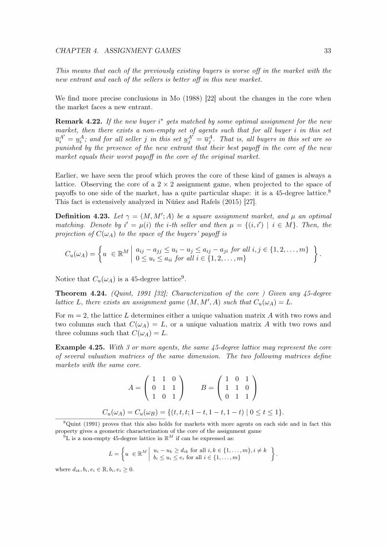
Example 4.25. With 3 or more agents, the same 45-degree lattice may represent the coreof several valuation matrices of the same dimension. The two following matrices definemarkets with the same core.
A =
1 1 00 1 11 0 1
B =
1 0 11 1 00 1 1
Cu(ωA) = Cu(ωB) = {(t, t, t; 1− t, 1− t, 1− t) | 0 ≤ t ≤ 1}.
8Quint (1991) proves that this also holds for markets with more agents on each side and in fact thisproperty gives a geometric characterization of the core of the assignment game
9L is a non-empty 45-degree lattice in RM if can be expressed as:
L =
{u ∈ RM
∣∣∣∣ ui − uk ≥ dik for all i, k ∈ {1, . . . ,m}, i 6= kbi ≤ ui ≤ ei for all i ∈ {1, . . . ,m}
}.
where dik, bi, ei ∈ R, bi, ei ≥ 0.
CHAPTER 4. ASSIGNMENT GAMES 34
Quint (1991) [32] poses the question of which is the maximum matrix A among thosematrices with C(ωA) = L, given a 45-degree lattice L. Clearly, this maximality requiresthat no matrix entry can be raised without modifying the core, that is, for each (i, j) ∈M ×M ′ there must be a core element (u, v) ∈ C(ωA) with ui + vj = aij . This is a weakerform of exactness10.
Theorem 4.26. A square assignment game (M∪M ′, ωA), with an optimal matching placedon the main diagonal, is exact if and only if matrix A has:
• a dominant diagonal: aii ≥ aij and aii ≥ aji, for all i, j ∈M and
• a doubly dominant diagonal: aij + akk ≥ aij + ajk, for all i, j, k ∈M .
Proof. The reader is referred to Solymosi and Raghavan (2001) [37].
If an assignment game is exact, its valuation matrix is maximum among those leading tothe same core.
Theorem 4.27. Given an assignment game (M ∪M ′, ωA), there exists a unique matrixA that is buyer-seller exact and give rise to the same core, C(ωA) = C(ωA).
Proof. The theorem above is proved in Núñez and Rafels (2002a) [24].
In Núñez and Rafels (2002a) [24], under the assumption that A is square and µ an optimalmatching, for all (i, j) ∈M ×M ′, the entry in A is given by
aij = aiµ(i) + aµ−1(j)j + ωA(M ∪M ′ \ {µ−1(j), µ(i)}
)− ωA(M ∪M ′).
Corollary 4.28. An assignment game (M ∪M ′, ωA) is buyer-seller exact if and only if Ahas a doubly dominant diagonal.
Example 4.29. The buyer-seller exact representative of matrices A and B in Example4.25 is the matrix with entries aij = 1 for all i, j = 1, 2, 3. This is a glove market, of thesame type that the one mentioned in Example 2.5.
10A coalitional game (N, v) is exact if for all S ⊂ N there exists x ∈ C(v) such that∑i∈S xi = v(S).
CHAPTER 4. ASSIGNMENT GAMES 35
4.5 Buyer and seller optima
In 1982/83 Leonard [18] and Demange [9] discovered independently from each other asimple procedure to find the buyer or seller optimum of an assignment market. We willexplain this procedure briefly, and first we will explain what this concept means.
Let (M,M ′;A) be an assignment market and (M ∪M ′, ωA) be its associated assignmentgame. We start with calculating the maximum payoff each buyer j in the core can receive.This is equal to vj , and Leonard and Demange prove that it is the value that buyer j addsto the grand coalition N = M ∪M ′ in case he joins as the last member:
vj = ωA(N)− ωA(N\{j}) ∀j ∈M ′.
Roth and Sotomayor [33] have a rather simpler proof to show this equality. Once eachbuyer received his maximum payoff, it easy to determine the minimum payoff for eachseller i hence for any optimal assignment µ the equation ui + vµ(i) = aiµ(i) holds true.Hence each seller i receives
ui = aiµ(i) − vµ(i) = aiµ(i) − ωA(N) + ωA(N\{µ(i)}) ∀i ∈M.
To calculate the seller optimum we use the same procedure but starting with calculatingthe sellers’ maximum payoffs
ui = ωA(N)− ωA(N\i) ∀i ∈M ,
and afterward the buyers’ minimum payoffs
vj = aµ−1(j)j − uµ−1(j) = aµ−1(j)j − ωA(N) + ωA(N\µ−1(j)) ∀j ∈M ′.
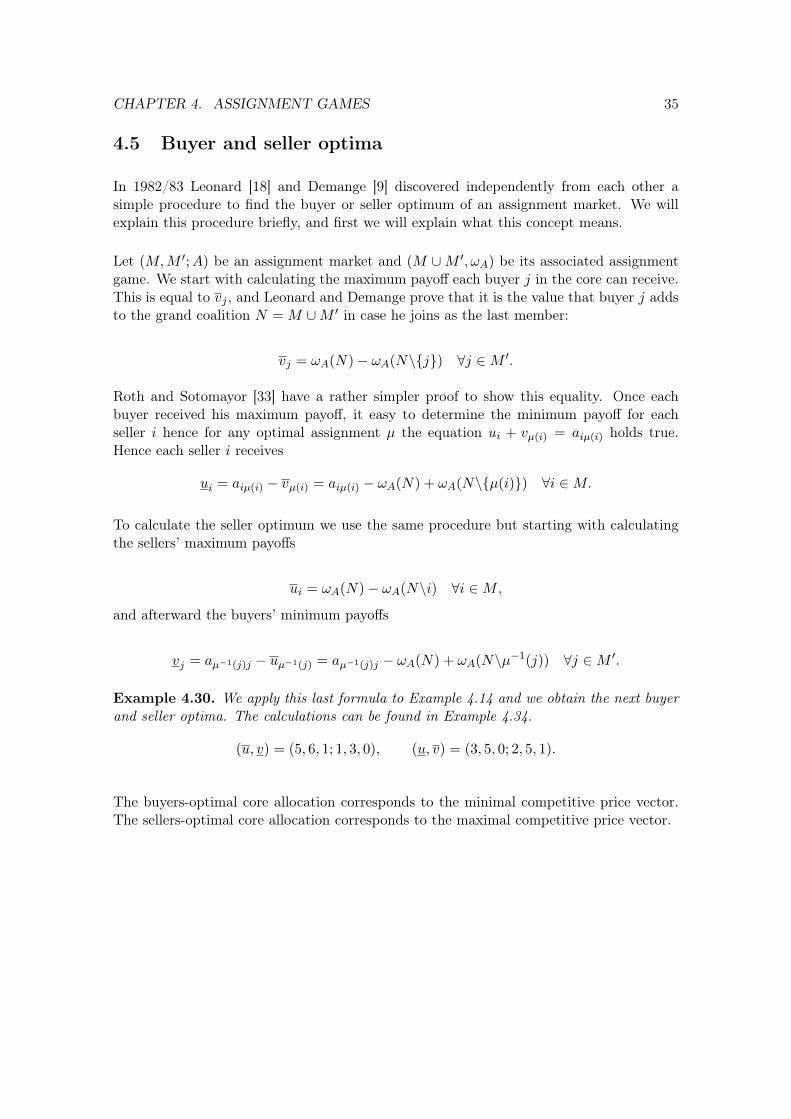
Example 4.30. We apply this last formula to Example 4.14 and we obtain the next buyerand seller optima. The calculations can be found in Example 4.34.
(u, v) = (5, 6, 1; 1, 3, 0), (u, v) = (3, 5, 0; 2, 5, 1).
The buyers-optimal core allocation corresponds to the minimal competitive price vector.The sellers-optimal core allocation corresponds to the maximal competitive price vector.

CHAPTER 4. ASSIGNMENT GAMES 36
4.6 The extreme core allocations of the assignment game
The core of a cooperative game can be described with a set of equalities and inequalitiesand it is always a compact and convex set. Therefore it can also be described by its extremepoints. There does not exist a simple procedure to find these extreme points in general.Due to the special form of the core of the assignment game, it is a lattice, there existsa quite intuitive way, similarly to the finding of the sellers-optimal and buyers-optimalallocation, to find the extreme allocations of the core of the assignment game.
Núñez and Rafels (2003) [26] shows that the set of extreme core allocations of the assign-ment game coincides with the set of reduced marginal worth vectors. It is a complex butcomplete procedure to calculate the set of reduced marginal worth vectors11. However, in2007, Izquierdo, Núñez and Rafels [15] discovered another and simpler method to calculatethe extreme core allocations of an assignment game.
To this end, let us introduce a set of vectors called max-payoff vectors. with one max-payoffvector xθ(A) for each possible ordering of the agents. An ordering θ = (k1, k2, . . . , kn) is
a bijection from N = M ∪ M ′ to N = M ∪ M ′. Each agent ki ∈ N is assigned toa position i ∈ {1, 2, . . . , n}. The function θ(i) returns agent ki for all i ∈ N and theinverse function θ−1(ki) = i gives back the position i for each agent ki ∈ N . The set oforderings on N is called Θ. The set of antecessors of an agent k ∈ N in the ordering θ isP θk = {j ∈M ∪M ′|θ−1(j) < θ−1(k)}.
Definition 4.31. Given an assignment game (M ∪M ′, ωA) we recursively define a payoffvector xθ(A) ∈ RM × RM ′, named a max-payoff vector, for each possible order θ on theplayer set in the following way: xθk1(A) = 0 and
xθkr(A) =
maxi∈P θkr∩M{0, aikr − xθi (A)} if kr ∈M ′,
maxj∈P θkr∩M′{0, akrj − xθj(A)} if kr ∈M .
Example 4.32. As an exercise, take the order θ = (1, 2′, 1′, 2) on the player set of the as-signment game of Example 4.13. The associated max-payoff vector is xθ1(A) = 0, xθ2′(A) =max{0, 4−0} = 4, xθ1′(A) = max{0, 5−0} = 5 and xθ2(A) = max{0, 2−5, 3−4} = 0. Thenxθ(A) = (0, 0, 5, 4). It is not efficient, which is not surprising since A has not a dominantdiagonal. Some other orders, take for instance θ′ = (2, 2′, 1, 1′), lead to an extreme corepoint.
The total number of orderings |Θ| = (m+m′)! is large even for small games. It is possibleto reduce to the number of required orderings to a subset Θµ. Here each buyer or seller
11Given a coalitional game (N, v) and any order k on the player set N , the marginal worth vectormk,v ∈ RN pays each agent his/her contribution to the set of predecessors according to the order k. Thatis, mk,v
k(1) = v({k(1)}) and, for all i ∈ {2, . . . , n},
mk,vk(i) = v({k(1), . . . , k(i)})− v({k(1), . . . , k(i− 1)})

CHAPTER 4. ASSIGNMENT GAMES 37
who occupies an odd number is followed by his optimal match, i.e. for µ ∈M∗A(M,M ′):
Θµ =
θ = (k1, . . . , kn) ∈ Θ
∣∣∣∣∣∣for all r ∈
{0, 1, 2, . . . , n2 − 1
}if k2r+1 ∈M then k2r+2 = µ(k2r+1)if k2r+1 ∈M ′ then k2r+2 = µ−1(k2r+1)
.
The number of required orderings |Θµ| for an assignment game with an equal numberof buyers and sellers (m = m′) still increases rapidly since there are m optimal buyer-seller pairs, hence m! different pair orderings. Each optimal pair can be switched around(k, µ(k)) → (µ(k), k) thus another 2m different combinations are possible. If we combinethese two numbers we obtain the number of orderings:
|Θµ| = m!× 2m.
This number is already much smaller than the total number of orderings |Θ| = (2m)! butstill quite large. To show the increasing number of orderings, we calculate the number oforderings for games with different size. It becomes quite obvious that for large games e.g.a used car market with 30 different cars the max-payoff vectors are so numerous that itbecomes impossible to calculate them.
Table 4.1: Number of Orderings |Θµ| and |Θ|m |Θµ| |Θ|1 2 2
2 8 24
3 48 720
4 384 40, 320
5 3, 840 3, 628, 800
6 46, 080 479, 001, 600
7 645, 120 87, 178, 291, 200
8 10, 321, 920 20, 922, 789, 888, 000
9 185, 794, 560 6.402, 373, 705, 728, 000
10 3, 715, 891, 200 2, 432, 902, 008, 176, 640, 000
11 81, 749, 606, 400 1, 124, 000, 727, 777, 607, 680, 000
12 1, 961, 990, 553, 600 620, 448, 401, 733, 239, 439, 360, 000
Izquierdo, Núñez, and Rafels [15] prove that max-payoff vectors are not, in general, efficientand that only the efficient max-payoff vectors are extreme core allocations.
Theorem 4.33. Let (M ∪M ′, ωA) be an assignment game with an equal number of buyersand sellers and let µ∗ be an optimal matching, µ∗ ∈M∗A(M,M ′). Then,
Ext(C(ωA)) = {xθ | θ ∈ Θµ, xθi + xθj = aij for all (i, j) ∈ µ∗}.
This is a full characterization of the extreme core allocations and therefore closes the searchfor the extreme points.
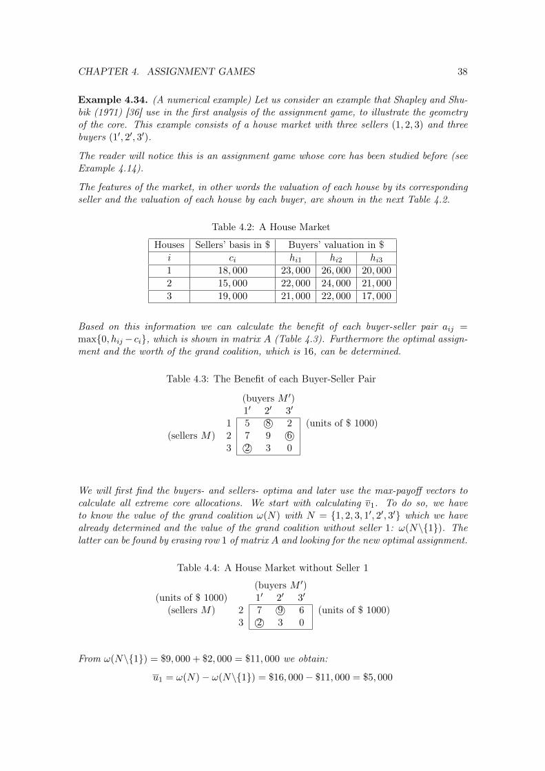
CHAPTER 4. ASSIGNMENT GAMES 38
Example 4.34. (A numerical example) Let us consider an example that Shapley and Shu-bik (1971) [36] use in the first analysis of the assignment game, to illustrate the geometryof the core. This example consists of a house market with three sellers (1, 2, 3) and threebuyers (1′, 2′, 3′).
The reader will notice this is an assignment game whose core has been studied before (seeExample 4.14).
The features of the market, in other words the valuation of each house by its correspondingseller and the valuation of each house by each buyer, are shown in the next Table 4.2.
Table 4.2: A House Market
Houses Sellers’ basis in $ Buyers’ valuation in $i ci hi1 hi2 hi31 18, 000 23, 000 26, 000 20, 000
2 15, 000 22, 000 24, 000 21, 000
3 19, 000 21, 000 22, 000 17, 000
Based on this information we can calculate the benefit of each buyer-seller pair aij =max{0, hij− ci}, which is shown in matrix A (Table 4.3). Furthermore the optimal assign-ment and the worth of the grand coalition, which is 16, can be determined.
Table 4.3: The Benefit of each Buyer-Seller Pair
(buyers M ′)1′ 2′ 3′
1 5 8© 2 (units of $ 1000)(sellers M) 2 7 9 6©
3 2© 3 0
We will first find the buyers- and sellers- optima and later use the max-payoff vectors tocalculate all extreme core allocations. We start with calculating v1. To do so, we haveto know the value of the grand coalition ω(N) with N = {1, 2, 3, 1′, 2′, 3′} which we havealready determined and the value of the grand coalition without seller 1: ω(N\{1}). Thelatter can be found by erasing row 1 of matrix A and looking for the new optimal assignment.
Table 4.4: A House Market without Seller 1
(buyers M ′)(units of $ 1000) 1′ 2′ 3′
(sellers M) 2 7 9© 6 (units of $ 1000)3 2© 3 0
From ω(N\{1}) = $9, 000 + $2, 000 = $11, 000 we obtain:
u1 = ω(N)− ω(N\{1}) = $16, 000− $11, 000 = $5, 000
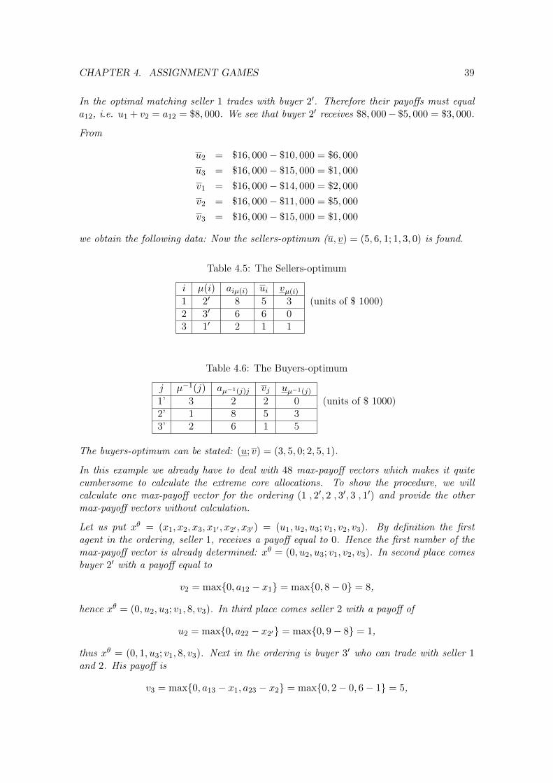
CHAPTER 4. ASSIGNMENT GAMES 39
In the optimal matching seller 1 trades with buyer 2′. Therefore their payoffs must equala12, i.e. u1 + v2 = a12 = $8, 000. We see that buyer 2′ receives $8, 000− $5, 000 = $3, 000.
From
u2 = $16, 000− $10, 000 = $6, 000
u3 = $16, 000− $15, 000 = $1, 000
v1 = $16, 000− $14, 000 = $2, 000
v2 = $16, 000− $11, 000 = $5, 000
v3 = $16, 000− $15, 000 = $1, 000
we obtain the following data: Now the sellers-optimum (u, v) = (5, 6, 1; 1, 3, 0) is found.
Table 4.5: The Sellers-optimum
i µ(i) aiµ(i) ui vµ(i)
1 2′ 8 5 3 (units of $ 1000)2 3′ 6 6 03 1′ 2 1 1
Table 4.6: The Buyers-optimum
j µ−1(j) aµ−1(j)j vj uµ−1(j)
1’ 3 2 2 0 (units of $ 1000)2’ 1 8 5 33’ 2 6 1 5
The buyers-optimum can be stated: (u; v) = (3, 5, 0; 2, 5, 1).
In this example we already have to deal with 48 max-payoff vectors which makes it quitecumbersome to calculate the extreme core allocations. To show the procedure, we willcalculate one max-payoff vector for the ordering (1 , 2′, 2 , 3′, 3 , 1′) and provide the othermax-payoff vectors without calculation.
Let us put xθ = (x1, x2, x3, x1′ , x2′ , x3′) = (u1, u2, u3; v1, v2, v3). By definition the firstagent in the ordering, seller 1, receives a payoff equal to 0. Hence the first number of themax-payoff vector is already determined: xθ = (0, u2, u3; v1, v2, v3). In second place comesbuyer 2′ with a payoff equal to
v2 = max{0, a12 − x1} = max{0, 8− 0} = 8,
hence xθ = (0, u2, u3; v1, 8, v3). In third place comes seller 2 with a payoff of
u2 = max{0, a22 − x2′} = max{0, 9− 8} = 1,
thus xθ = (0, 1, u3; v1, 8, v3). Next in the ordering is buyer 3′ who can trade with seller 1and 2. His payoff is
v3 = max{0, a13 − x1, a23 − x2} = max{0, 2− 0, 6− 1} = 5,
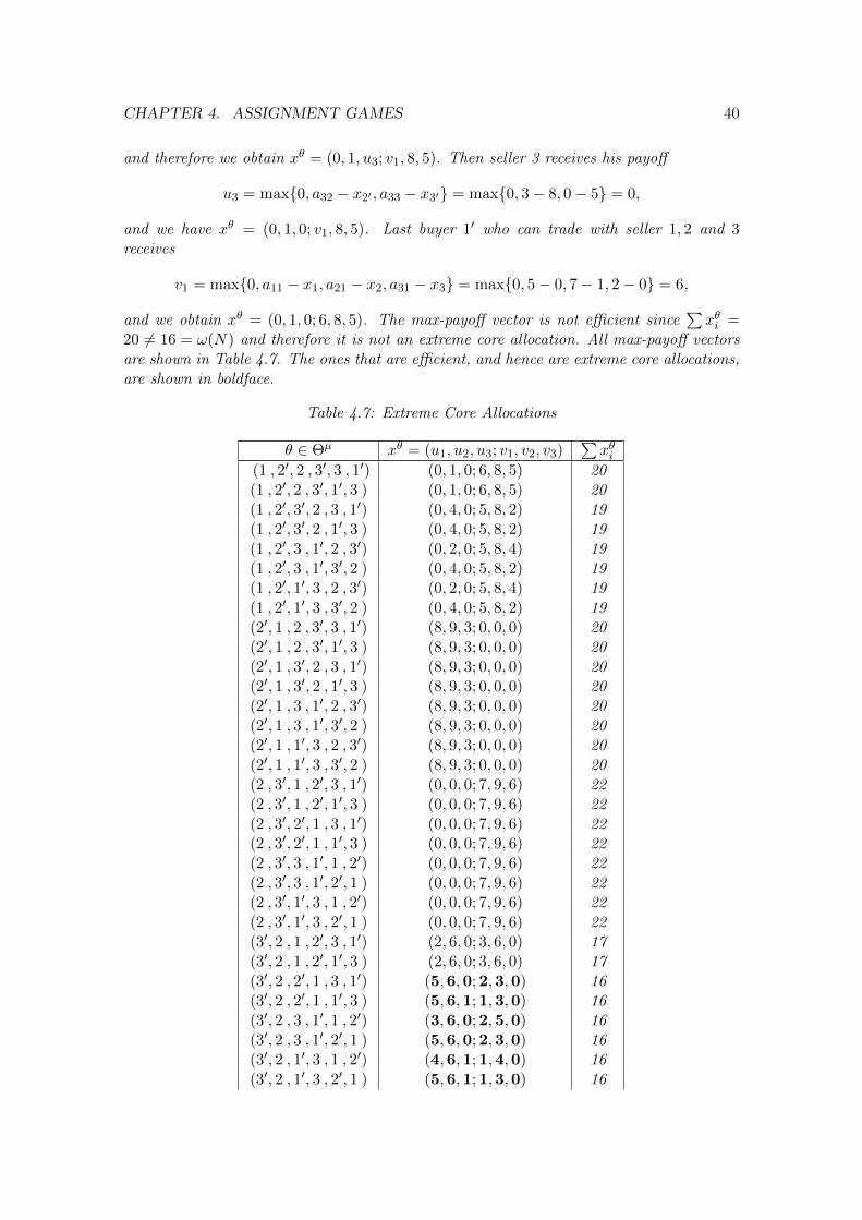
CHAPTER 4. ASSIGNMENT GAMES 40
and therefore we obtain xθ = (0, 1, u3; v1, 8, 5). Then seller 3 receives his payoff
u3 = max{0, a32 − x2′ , a33 − x3′} = max{0, 3− 8, 0− 5} = 0,
and we have xθ = (0, 1, 0; v1, 8, 5). Last buyer 1′ who can trade with seller 1, 2 and 3receives
v1 = max{0, a11 − x1, a21 − x2, a31 − x3} = max{0, 5− 0, 7− 1, 2− 0} = 6,
and we obtain xθ = (0, 1, 0; 6, 8, 5). The max-payoff vector is not efficient since∑xθi =
20 6= 16 = ω(N) and therefore it is not an extreme core allocation. All max-payoff vectorsare shown in Table 4.7. The ones that are efficient, and hence are extreme core allocations,are shown in boldface.
Table 4.7: Extreme Core Allocations
θ ∈ Θµ xθ = (u1, u2, u3; v1, v2, v3)∑xθi
(1 , 2′, 2 , 3′, 3 , 1′) (0, 1, 0; 6, 8, 5) 20(1 , 2′, 2 , 3′, 1′, 3 ) (0, 1, 0; 6, 8, 5) 20(1 , 2′, 3′, 2 , 3 , 1′) (0, 4, 0; 5, 8, 2) 19(1 , 2′, 3′, 2 , 1′, 3 ) (0, 4, 0; 5, 8, 2) 19(1 , 2′, 3 , 1′, 2 , 3′) (0, 2, 0; 5, 8, 4) 19(1 , 2′, 3 , 1′, 3′, 2 ) (0, 4, 0; 5, 8, 2) 19(1 , 2′, 1′, 3 , 2 , 3′) (0, 2, 0; 5, 8, 4) 19(1 , 2′, 1′, 3 , 3′, 2 ) (0, 4, 0; 5, 8, 2) 19(2′, 1 , 2 , 3′, 3 , 1′) (8, 9, 3; 0, 0, 0) 20(2′, 1 , 2 , 3′, 1′, 3 ) (8, 9, 3; 0, 0, 0) 20(2′, 1 , 3′, 2 , 3 , 1′) (8, 9, 3; 0, 0, 0) 20(2′, 1 , 3′, 2 , 1′, 3 ) (8, 9, 3; 0, 0, 0) 20(2′, 1 , 3 , 1′, 2 , 3′) (8, 9, 3; 0, 0, 0) 20(2′, 1 , 3 , 1′, 3′, 2 ) (8, 9, 3; 0, 0, 0) 20(2′, 1 , 1′, 3 , 2 , 3′) (8, 9, 3; 0, 0, 0) 20(2′, 1 , 1′, 3 , 3′, 2 ) (8, 9, 3; 0, 0, 0) 20(2 , 3′, 1 , 2′, 3 , 1′) (0, 0, 0; 7, 9, 6) 22(2 , 3′, 1 , 2′, 1′, 3 ) (0, 0, 0; 7, 9, 6) 22(2 , 3′, 2′, 1 , 3 , 1′) (0, 0, 0; 7, 9, 6) 22(2 , 3′, 2′, 1 , 1′, 3 ) (0, 0, 0; 7, 9, 6) 22(2 , 3′, 3 , 1′, 1 , 2′) (0, 0, 0; 7, 9, 6) 22(2 , 3′, 3 , 1′, 2′, 1 ) (0, 0, 0; 7, 9, 6) 22(2 , 3′, 1′, 3 , 1 , 2′) (0, 0, 0; 7, 9, 6) 22(2 , 3′, 1′, 3 , 2′, 1 ) (0, 0, 0; 7, 9, 6) 22(3′, 2 , 1 , 2′, 3 , 1′) (2, 6, 0; 3, 6, 0) 17(3′, 2 , 1 , 2′, 1′, 3 ) (2, 6, 0; 3, 6, 0) 17(3′, 2 , 2′, 1 , 3 , 1′) (5,6,0;2,3,0) 16(3′, 2 , 2′, 1 , 1′, 3 ) (5,6,1;1,3,0) 16(3′, 2 , 3 , 1′, 1 , 2′) (3,6,0;2,5,0) 16(3′, 2 , 3 , 1′, 2′, 1 ) (5,6,0;2,3,0) 16(3′, 2 , 1′, 3 , 1 , 2′) (4,6,1;1,4,0) 16(3′, 2 , 1′, 3 , 2′, 1 ) (5,6,1;1,3,0) 16
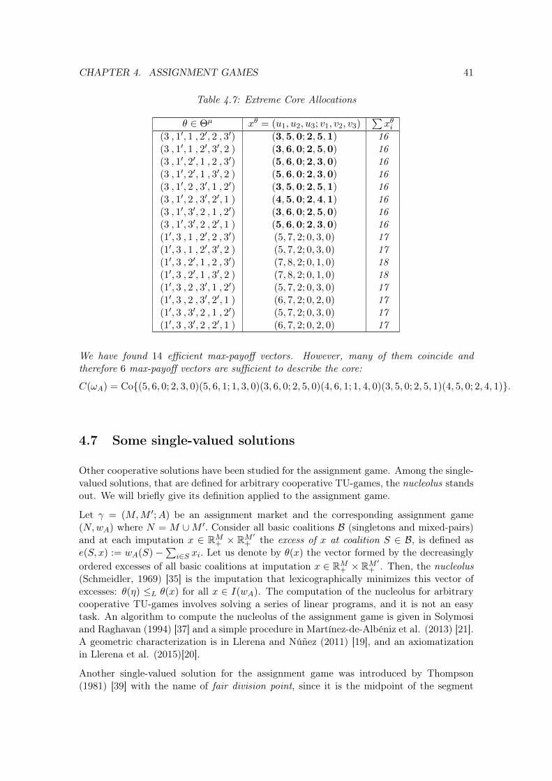
CHAPTER 4. ASSIGNMENT GAMES 41
Table 4.7: Extreme Core Allocations
θ ∈ Θµ xθ = (u1, u2, u3; v1, v2, v3)∑xθi
(3 , 1′, 1 , 2′, 2 , 3′) (3,5,0;2,5,1) 16(3 , 1′, 1 , 2′, 3′, 2 ) (3,6,0;2,5,0) 16(3 , 1′, 2′, 1 , 2 , 3′) (5,6,0;2,3,0) 16(3 , 1′, 2′, 1 , 3′, 2 ) (5,6,0;2,3,0) 16(3 , 1′, 2 , 3′, 1 , 2′) (3,5,0;2,5,1) 16(3 , 1′, 2 , 3′, 2′, 1 ) (4,5,0;2,4,1) 16(3 , 1′, 3′, 2 , 1 , 2′) (3,6,0;2,5,0) 16(3 , 1′, 3′, 2 , 2′, 1 ) (5,6,0;2,3,0) 16(1′, 3 , 1 , 2′, 2 , 3′) (5, 7, 2; 0, 3, 0) 17(1′, 3 , 1 , 2′, 3′, 2 ) (5, 7, 2; 0, 3, 0) 17(1′, 3 , 2′, 1 , 2 , 3′) (7, 8, 2; 0, 1, 0) 18(1′, 3 , 2′, 1 , 3′, 2 ) (7, 8, 2; 0, 1, 0) 18(1′, 3 , 2 , 3′, 1 , 2′) (5, 7, 2; 0, 3, 0) 17(1′, 3 , 2 , 3′, 2′, 1 ) (6, 7, 2; 0, 2, 0) 17(1′, 3 , 3′, 2 , 1 , 2′) (5, 7, 2; 0, 3, 0) 17(1′, 3 , 3′, 2 , 2′, 1 ) (6, 7, 2; 0, 2, 0) 17
We have found 14 efficient max-payoff vectors. However, many of them coincide andtherefore 6 max-payoff vectors are sufficient to describe the core:
C(ωA) = Co{(5, 6, 0; 2, 3, 0)(5, 6, 1; 1, 3, 0)(3, 6, 0; 2, 5, 0)(4, 6, 1; 1, 4, 0)(3, 5, 0; 2, 5, 1)(4, 5, 0; 2, 4, 1)}.
4.7 Some single-valued solutions
Other cooperative solutions have been studied for the assignment game. Among the single-valued solutions, that are defined for arbitrary cooperative TU-games, the nucleolus standsout. We will briefly give its definition applied to the assignment game.
Let γ = (M,M ′;A) be an assignment market and the corresponding assignment game(N,wA) where N = M ∪M ′. Consider all basic coalitions B (singletons and mixed-pairs)and at each imputation x ∈ RM+ × RM ′+ the excess of x at coalition S ∈ B, is defined ase(S, x) := wA(S)−
∑i∈S xi. Let us denote by θ(x) the vector formed by the decreasingly
ordered excesses of all basic coalitions at imputation x ∈ RM+ × RM ′+ . Then, the nucleolus(Schmeidler, 1969) [35] is the imputation that lexicographically minimizes this vector ofexcesses: θ(η) ≤L θ(x) for all x ∈ I(wA). The computation of the nucleolus for arbitrarycooperative TU-games involves solving a series of linear programs, and it is not an easytask. An algorithm to compute the nucleolus of the assignment game is given in Solymosiand Raghavan (1994) [37] and a simple procedure in Martínez-de-Albéniz et al. (2013) [21].A geometric characterization is in Llerena and Núñez (2011) [19], and an axiomatizationin Llerena et al. (2015)[20].
Another single-valued solution for the assignment game was introduced by Thompson(1981) [39] with the name of fair division point, since it is the midpoint of the segment
CHAPTER 4. ASSIGNMENT GAMES 42
between the buyers-optimal and the sellers-optimal core allocation. If (M ∪M ′, wA) is anassignment game, the fair division point is given by
τ(wA) = 12(uA, vA) + 1
2(uA, vA).
Nuñez and Rafels (2002b) [25] proves that the fair division point coincides with the τ -value(Tijs, 1981) [38].
Chapter 5
Multi-item auctions
As seen in Chapter 4, the core of the assignment game coincides with the competitiveequilibria of the assignment market. There is a one-to-one correspondence between eachcore allocation and competitive prices. A very natural question arises from this fact, if itis possible to design a mechanism (non-cooperative in nature) such that the equilibrium ofthe associated non-cooperative game correspond to some of these competitive equilibria1.In particular we care about the buyers-optimal core allocation.
5.1 Multi-item auction mechanism
In this section we describe a mechanism to determine the buyers-optimal core allocationgiven the data of the market. The question above is addressed in Demange et al. (1986)[10]. Studies by Demange (1982) [9], Leonard (1983) [18] and Gale and Demange (1985) [12]consider an allocation mechanism that turns out to be a generalization of the well-known“second-price2” auction first described by Vickrey (1961) [41].
In order to describe the multi-item generalization of this mechanism it is convenient tothink of the second-price scheme as an ordinary competitive equilibrium, when there isonly one item on sale. The most important property of the second highest bid is that it isthe smallest equilibrium price since for any smaller price at least two bidders would demandthe item. In the multi-item generalization it is assumed that each bidder is interested inacquiring at most one item, as might be the case if, for example, the auction was designedto assign individuals to positions, as considered by Leonard (1983) [18].
The multi-item auction mechanism requires each bidder (buyer) to submit in a sealed bidlisting his valuation of all the items. The auctioneer then allocates the items in accordancewith the minimum price equilibrium.
A main point of the papers cited is that the important “incentive capability” of the single-item auction carries over to the multi-item case, meaning that submitting true valuation is
1Reader can check the definition of competitive equilibrium in Definition 4.10.2In this auction, the participants submit sealed bids for a single item. That item is sold to the highest
bidder at a price equal to the second highest bid.
43

CHAPTER 5. MULTI-ITEM AUCTIONS 44
a dominant strategy for the bidders. Therefore, by jointly falsifying valuations, no subsetof bidders can improve the outcome for all its members.
In this chapter we are going to study the exact auction mechanism from Demange et al.(1986) [10] applied to a second-price auction.
Clearly, a second-price auction can be read into as an assignment game within the nextframework.
• A finite set Nof agents and a finite set O′of indivisible objects.
• The finite set of objects O ⊂ N that includes O′ and as many copies of a null objectas agents in N. This null object is denoted by ∅.
• Each i ∈ N can acquire at most one object and each i ∈ N has a valuation aij ∈ R+
for each j ∈ O. Null objects have a valuation of zero.
• Agent i’s valuation ai = (aij)j∈O ∈ A and a valuation profile a = (ai)i∈N ∈ ANwhere AN = A× ...×A.
• An assignment µ = (µi)i∈N is a vector that assigns µi ∈ O to i and each object isassigned at most to one agent.
• LetM(S,Q) be the set of all allocations of objects Q ⊆ O to agents S ⊆ N .
• A price vector is p ∈ RO+ such that p∅ = 0 for each ∅.
Thus, as we can see, we have an assignment problem where the question is how to assignobjects to agents in the best possible way. In Vickrey (1961) [41], it is shown a mechanismto find the maximum competitive equilibrium and the minimum competitive equilibriumunder certain circumstances: the gross-substitutes (GS) condition3 and quasi-linear prefer-ences4.
In other words, the GS condition supposes that given an initial price vector, an agentwants to consume a bundle of objects. Assume that some prices increase and considers anew vector of prices, then the agent still wants to consume those objects belonging to thebundle with the same price in both price vectors. This is exactly what is happening inthe framework above. The quasi-linear preferences are satisfied by the assignment gamewe are considering. We have seen in Chapter 4 that competitive equilibrium price vectorsof an assignment game belong to the core of the assignment game. And we have also seenthat the core of the assignment game is non-empty and forms a complete lattice.
Once checked these two conditions, it is possible to apply which is known as VCG mech-anism5 to obtain the maximum competitive equilibrium and the minimum competitive
3A valuation ai = (aij)j∈O ∈ A satisfies gross-substitutes condition if, and only if, for every pricep ∈ RO+, every set S ∈ Di(p), and every q > p, q ∈ RO+, there is a set T ⊆ A with (S \A)∪T ∈ Di(p) whereA = {j : q(j) > p(j)}, j ∈ O.
4The set of competitive equilibrium price vectors of the market is non-empty and forms a completelattice.
5VCG mechanisms allow for the selection of a socially optimal outcome out of a set of possible out-comes in a Vickrey–Clarke-Groves (VCG) auction. This is a type of sealed-bid auction of multiple items.The auction is named after Vickrey (1961) [41], Clarke (1971) and Groves (1973) for their papers thatsuccessively generalized the idea. The VCG auction is a specific use of the more general VCG mechanism.
CHAPTER 5. MULTI-ITEM AUCTIONS 45
equilibrium.
This mechanism is not shown in this dissertation6 but two interesting results come outfrom this process.
• The payoff obtained via VCG belongs to the core of the assignment game.
• The payoff obtained via VCG is supported by the minimum competitive equilibriumin the replicated market.
The exact auction mechanism derived in order to find the best possible outcome for all theagents works as follows:
• Step 1: The auctioneer announces the initial price vector. Then, every agent “bids”by announcing which object or objects are in his demand set given the prices.
• Step t (t ≥ 2): If it is possible to allocate to each agent an object belonging to hisdemand set given the price vector, the algorithm stops. If no such allocation exists,then there is an overdemanded set of objects. The auctioneer chooses a minimaloverdemanded set of objects and raises the price of each object in the set by oneunit. The price of all other objects remain at the same level.
The example below represents the operating of this mechanism.
Example 5.1. Consider a second-price auction with a set of 3 agents {1, 2, 3} and a setof 3 objects {1′, 2′, 3′}. Suppose the valuations are a1 = (10, 9, 8), a2 = (10, 9, 4) anda3 = (10, 4, 2).
The auction begins, consider the initial price vector p1 = (0, 0, 0). The demand sets of theagents are:
• D1(p0) = {1′}, D2(p0) = {1′}, D3(p0) = {1′}.
Since there is an overdemanded set, the auctioneer raises the price. Consider now p1 =(1, 0, 0) (p1 > p0, satisfies the GS condition).
• D1(p1) = {1′, 2′}, D2(p1) = {1′, 2′}, D3(p1) = {1′}.
Notice that {1′} is not an overdemanded set because
|{i ∈ N |Di(p1) ⊆ {1′}}| = |{3}| = |{1′}|,
but, note that {1′, 2′} is overdemanded:
|{i ∈ N |Di(p1) ⊆ {1′, 2′}}| = |{1, 2, 3}| > |{1′, 2′}|.
Now prices in the overdemanded set are raised. Consider p2 = (2, 1, 0) (p2 > p1, satisfiesthe GS condition again).
• D1(p2) = {1′, 2′, 3′}, D2(p2) = {1′, 2′}, D3(p2) = {1′}.
Now we can assign object 1′ to agent 3, object 2′ to agent 2 and object 3′ to agent 1.
6Interested reader is referred to Vickrey (1961) [41].

Chapter 6
Conclusions
Matching markets is an active area of research. This research consists of the study ofresource allocation problems in which two sets of agents, or a set of agents and a set ofgoods, have to be assigned to one another in a way the respects the preferences of themarket participants. There are several types of allocation problems. For example, two-sided matching markets where prices cannot be used; markets without money where wedesire to assign or re-allocate indivisible goods; and assignment markets where we want tofind prices that clear markets for potentially distinct and heterogeneous indivisible goods.
These are marriage markets, college admission problem, roommate problem, dependingon the precise characteristics of preferences, and so on. There are mechanisms that havebeen succesfully applied for the allocation of students to universities, resident doctors tohospitals (see Roth and Sotomayor (1990) [33]) or kidneys to patients in need of a transplant(Roth et al. (2005) [34]).
In this dissertation we have focused on markets with money, that is markets where pref-erences are quasilinear in money, and agents ask for one unit each. Money is the commonutility for all agents.
These markets allow the modeling of auctions of multiple objects (Demange et al. (1986)[10]) as it has been introduced in Chapter 5: Multi-items auctions. In the case of auctionswhere agents are allowed to bid for bundles of objects, it is also possible to model throughthe assignment markets. For instance, licenses for mobile telephony in different stateswhich are represented by what is known as package assignment game (Bikhchandani andOstroy (2002) [1]).
The multi-item auction model seen in this project is “unsymmetrical” which means thateach seller specifies only one number, his reservation price, while buyers specify theirvaluations for each of the items. There are, however, economically natural situations inwhich sellers “discriminate” specifying different reservation prices to different buyers. Thejob assignment problem is an example of this situation. Here the sellers are workers whoare selling their services to employers. Clearly, the minimum salary a worker would acceptmight vary depending on the job; for example, the more disagreeable the job, the higherthe minimum acceptable salary.
47
CHAPTER 6. CONCLUSIONS 48
The model of the assignment game, as defined by Shapley and Shubik (1971) [36], relies onseveral economic assumptions: there are two sides in the market, utility is identified withmoney, side-payments are allowed and the supply of each seller and the demand of eachbuyer are unitary. We could consider two different extensions that follow from relaxingthe two-sided nature of the market and the unitary demand and supply of the agents. Itresults that some of the nice properties and structure of solutions do not hold when weconsider these generalized assignment markets. The extension of the assignment marketwith multiple sides and multiple partners is called multi-sided assignment markets and isstudied in Núñez and Rafels (2015) [27].
Bibliography
[1] Bikhchandani, S., Ostroy J.M. (2002). The package assignment model. J Econ Theory,107:377–406.
[2] Birkhoff, G. (1946). Tres observaciones sobre el álgebra lineal. Rev Univ Nac Tucumán,Series A 5, 147–151.
[3] Birkhoff, G. (1973). Lattice theory. 3rd edition, AMS, Providence.
[4] Borm, P., Hamers, H., Hendrickx, R. (2001). Operations research games: a survey.TOP 9:139–216.
[5] Burkard, R., Dell’Amico. M., Martello, S. (2009). Assignment Problems. Society forIndustrial and Applied Mathematics, Philadelphia.
[6] Cariñena, J., Gràcia, X., Martínez, E., Muñoz, M., Marmo, G., Román-Roy N. (2006).Geometric Hamilton-Jacobi theory, International Journal of Geometric Methods inModern Physics, Volume 03.
[7] Curiel, I. (1997). Cooperative game theory and applications. Cooperative games aris-ing from combinatorial optimization problems. Kluwer Academic Publishers, Boston.
[8] Dantzig, G.B. (1963). Linear programming and extensions. Princeton University Press,Princeton.
[9] Demange, G. (1982). Strategyproofness in the assignment market game, mimeo, Lab-oratoire d’économetrie de l’École Polytechnique, Paris.
[10] Demange, G., Gale, D., Sotomayor, M. (1986). Multi-Item Auctions. Journal of Po-litical Economy 94(4):863–872.
[11] Gale, D. (1960). The Theory of Linear Economic Models, University of Chicago Press,Chicago and London.
[12] Gale, D., Demange, G. (1985) The Strategy Structure of Two-sided Matching Markets.Econometrica 53(1):873–83.
[13] Gillies, D.B. (1959). Solutions to general non-zero-sum games. In H.W. Kuhn and A.W. Tucker (eds.), Contributions to the Theory of Games IV. Princeton UniversityPress, Princeton. pp. 47–85.
[14] González-Díaz, J., García-Jurado, I., Fiestras-Janeiro, M.G. (2010). An introductorycourse on mathematical game theory. American Mathematical Society / Real Sociedad
49

BIBLIOGRAPHY 50
Matemática Española, Graduate Studies in Mathematics, Volume 115.
[15] Izquierdo, J.M., Núñez, M., Rafels, C. (2007). A simple procedure to obtain theextreme core allocations of an assignment market. Int J Game Theory 36:17–26.
[16] Koopmans, T.C., Beckmann, M. (1957). Assignment problems and the location ofeconomic activities. Econometrica 25(1):53–76.
[17] Kuhn, H. W. (1955). The Hungarian method for the assignment problem. Naval ResLogistics (NRL) 52(1):7–21.
[18] Leonard, H. B. (1983). Elicitation of honest preferences for the assignment of individ-uals to positions. J Pol Econ 93(3):461–479.
[19] Llerena, F., Núñez, M. (2011). A geometric characterization of the nucleolus of theassignment game. Economics Bulletin, 31(4):3275–3285.
[20] Llerena, F., Núñez, M., Rafels, C. (2015). An axiomatization of the nucleolus ofassignment markets international Journal of Game Theory 44(1):1–15.
[21] Martínez-de-Albéniz, F.J., Rafels, C., Ybern, N. (2013). A procedure to compute thenucleolus of the assignment game. Oper Res Letters 41:675–678.
[22] Mo, J. P. (1988). Entry and structures of interest groups in assignment games. Eco-nomic Theory 46:66–96.
[23] Nash, J.F. (1951). Non-cooperative games. Annals of Mathematics 54(2):286–295.
[24] Núñez, M., Rafels, C. (2002a). Buyer-seller exactness in the assignment game. Int JGame Theory, 31(2):423–436.
[25] Núñez, M., Rafels, C. (2002b). The assignment game: the τ -value. Int J Game Theory,31(2):411–422.
[26] Núñez, M., Rafels, C. (2003). Characterization of the extreme core allocations of theassignment game. Games Econ Behav 44:311–331.
[27] Núñez, M., Rafels, C. (2015). A survey on assignment markets. Journal of Dynamicsand Games 2:227–256.
[28] Owen, G. (1972). Values of games without side payments. Int J Game Theory 1:95–109.
[29] Owen, G. (1975). On the core of linear production games. Math Programming 9:358–370.
[30] Peleg, B., Sudhölter, P. (2003). Introduction to the Theory of Cooperative Games.Springer-Verlag.
[31] Pentico, D.W. (2007). Assignment problems: A golden anniversary survey. Eur J OperResearch 176:774–793.
[32] Quint, T. (1991). Characterization of cores of assignment games. Int J Game Theory19:413–420.
[33] Roth, A.E., Sotomayor, M.A.O. (1990). Two-sided matching. Econometric Society
BIBLIOGRAPHY 51
Monographs, 18. Cambridge University Press.
[34] Roth, A.E., Sönmez, T., Ünver M.U. (2005). Pairwise kidney exchange. Journal ofEconomic Theory 125:151–188.
[35] Schmeidler, D. (1969). The nucleolus of a characteristic function game. SIAM Journalon Applied Mathematics 17:1163–1170.
[36] Shapley, L.S., Shubik, M. (1971). The assignment game I: The core. Int J GameTheory 1:111–130.
[37] Solymosi, T., Raghavan, T.E.S. (2001). Assignment games with stable core, Int JGame Theory 30:177–185.
[38] Tijs, S.H. (1981). Bounds for the core and the τ -value. In Game Theory and Mathe-matical Economics, O. Moeschlin and D. Pallaschke (eds.) North Holland PublishingCompany, pp. 123–132.
[39] Thompson, G.L. (1981). Auctions and market games. In: Essays in Game Theoryand Mathematical Economics in honor of Oskar Morgenstern. R. Aumann et al., eds.Bibliographisches Institut–Wissenschaftsverlag Mannheim, pp. 181–196.
[40] Vohra, R. (2005). Advanced mathematical economics. Routledge.
[41] Vickrey, W. (1961). Counterspeculation, auctions and competitive sealed tenders.Journal of Finance 6:8–37.
[42] von Neumann, J., Morgenstern O. (1944). The Theory of Games and Economic Be-havior. 2nd edition, Princeton University Press, Princeton.
[43] von Neumann, J. (1953). A certain zero-sum two-person game equivalent to the opti-mal assignment problem. In Contributions to the theory of games II, H.W. Kuhn (ed)Ann of Math Studies, 28, Princeton Univ Press, pp. 5–12.