AN ENGINEER’S GUIDE TO MATLAB 3rd Edition CHAPTER 2 VECTORS and MATRICES
117
Copyright © Edward B. Magrab 2009 1 Copyright © Edward B. Magrab 2009 Chapter 2 An Engineer’s Guide to MATLAB AN ENGINEER’S GUIDE TO MATLAB 3rd Edition CHAPTER 2 VECTORS and MATRICES
-
Upload
tashya-brady -
Category
Documents
-
view
40 -
download
0
description
AN ENGINEER’S GUIDE TO MATLAB 3rd Edition CHAPTER 2 VECTORS and MATRICES. Chapter 2 – Objective Introduce MATLAB syntax in the context of vectors and matrices and their manipulation. Topics. Definitions of Matrices and Vectors Creation of Vectors Creation of Matrices Dot Operations - PowerPoint PPT Presentation
Transcript of AN ENGINEER’S GUIDE TO MATLAB 3rd Edition CHAPTER 2 VECTORS and MATRICES

Copyright © Edward B. Magrab 2009 1Copyright © Edward B. Magrab 2009
Chapter 2An Engineer’s Guide to MATLAB
AN ENGINEER’S GUIDE TO MATLAB
3rd Edition
CHAPTER 2
VECTORS and MATRICES

Copyright © Edward B. Magrab 2009 2Copyright © Edward B. Magrab 2009
Chapter 2An Engineer’s Guide to MATLAB
Chapter 2 – Objective
Introduce MATLAB syntax in the context of vectors and matrices and their manipulation.

Copyright © Edward B. Magrab 2009 3Copyright © Edward B. Magrab 2009
Chapter 2An Engineer’s Guide to MATLAB
Topics
• Definitions of Matrices and Vectors
• Creation of Vectors
• Creation of Matrices
• Dot Operations
• Mathematical Operations with Matrices Addition and Subtraction Multiplication Determinants Matrix Inverse Solution of a System of Equations
Copyright © Edward B. Magrab 2009 4Copyright © Edward B. Magrab 2009
Chapter 2An Engineer’s Guide to MATLAB
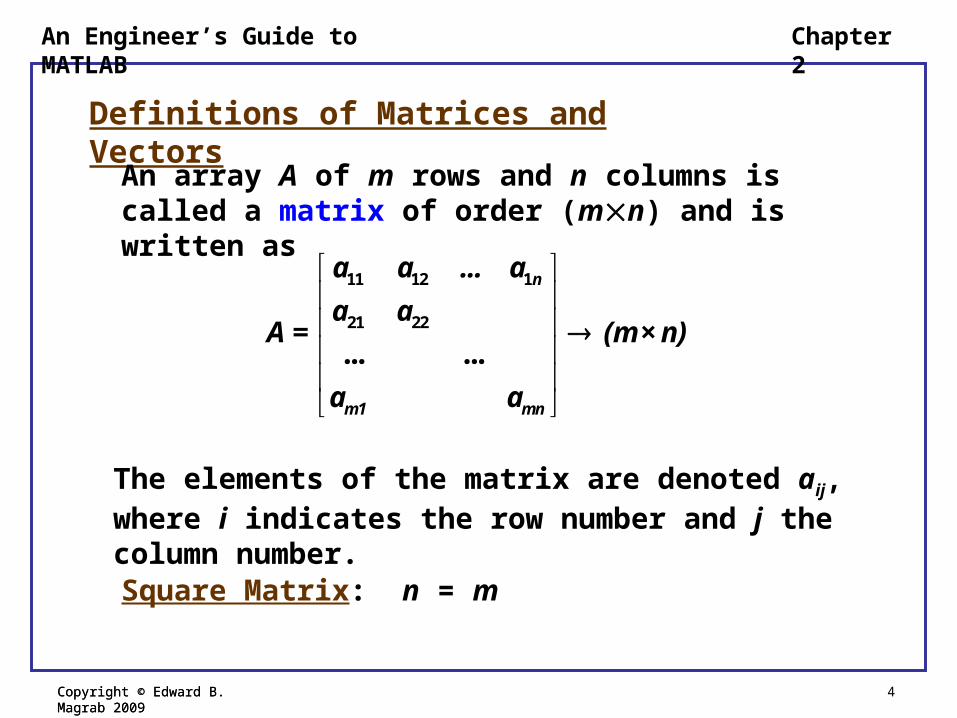
Definitions of Matrices and Vectors
An array A of m rows and n columns is called a matrix of order (mn) and is written as
11 12 1
21 22
... ...
n
m1 mn
a a ... a
a aA = (m×n)
a a
The elements of the matrix are denoted aij, where i indicates the row number and j the column number.
Square Matrix: n = m

Copyright © Edward B. Magrab 2009 5Copyright © Edward B. Magrab 2009
Chapter 2An Engineer’s Guide to MATLAB
Diagonal Matrix: When n = m and aij = 0, i ≠j; thus
11
22 ( )
0 ... 0
0
... ...
0 nn
a
aA = n n
a
Identity Matrix: Diagonal matrix with aii = 1; thus
1 0 ... 0
0 1=
... ...
0 1
I
Copyright © Edward B. Magrab 2009 6Copyright © Edward B. Magrab 2009
Chapter 2An Engineer’s Guide to MATLAB
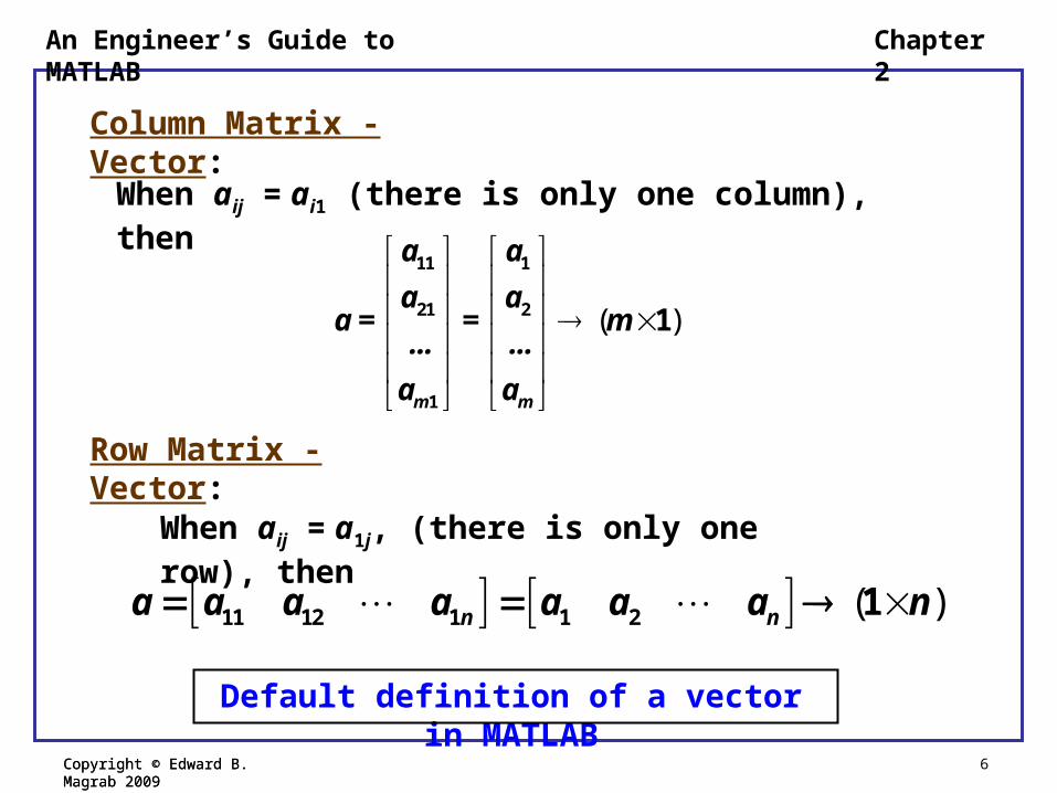
Column Matrix - Vector:
Row Matrix - Vector:
When aij = ai1 (there is only one column), then
( )
11 1
21 2
1
1
m m
a a
a aa = = m
... ...
a a
When aij = a1j, (there is only one row), then
( )11 12 1 1 2 1 n na a a a a a a n
Default definition of a vector in MATLAB

Copyright © Edward B. Magrab 2009 7Copyright © Edward B. Magrab 2009
Chapter 2An Engineer’s Guide to MATLAB
Transpose of a Matrix and a Vector
The transpose of a matrix is denoted by an apostrophe (). If A is defined as before and W = A, then
( )
11 11 12 21 1 1
21 12 22 22
1 1
m m
n n nm mn
w = a w = a ... w = a
w = a w = aW = A = n m
... ...
w = a w = a
11 12 1
21 22
... ...
n
m1 mn
a a ... a
a aA = (m×n)
a a
Recall that

Copyright © Edward B. Magrab 2009 8Copyright © Edward B. Magrab 2009
Chapter 2An Engineer’s Guide to MATLAB
For a row vector -
( ) ( )
1
21 2If ... 1 then 1
m
m
a
aa a a a m a m
a
1
21 2( ) ( )m
m
If 1 then ... 1...
a
aa m a a a a m
a
For a column vector -

Copyright © Edward B. Magrab 2009 9Copyright © Edward B. Magrab 2009
Chapter 2An Engineer’s Guide to MATLAB
If a, x, b, … are either variable names, numbers, expressions, or strings, then vectors are expressed as either
f = [a x b …] (Blanks required)
or
f = [a, x, b, …] (Blanks optional)
Creation of Vectors
Caution about blanks: If a = h + ds, then f is written as either
f = [h+d^s x b ...]
or
f = [h+d^s, x, b, ...]
No blanks permitted within expression

Copyright © Edward B. Magrab 2009 10Copyright © Edward B. Magrab 2009
Chapter 2An Engineer’s Guide to MATLAB
Ways to Assign Numerical Values to the Elements of a Vector -
• Specify the range of the values and the increment between adjacent values – called colon notation.
Used when the increment is either important or has been specified.
• Specify the range of the values and the number of values desired.
Used when the number of values is important.

Copyright © Edward B. Magrab 2009 11Copyright © Edward B. Magrab 2009
Chapter 2An Engineer’s Guide to MATLAB
If s, d, and f are any combination of numerical values, variable names, and expressions, then the colon notation that creates a vector x is either
x = s:d:f or x = (s:d:f) or x = [s:d:f]
where
s = start or initial valued = increment or decrementf = end or final value
Thus, the following row vector x is created
x = [s, s+d, s+2d, …, s+nd] (Note: s+nd f )

Copyright © Edward B. Magrab 2009 12Copyright © Edward B. Magrab 2009
Chapter 2An Engineer’s Guide to MATLAB
Also, when d is omitted MATLAB assumes that d = 1. Then
x = s:f
creates the vector
x = [s, s+1, s+2, … , s+n]
where s+n f
The number of terms, called the length of the vector, that this expression has created is determined from
length(x)

Copyright © Edward B. Magrab 2009 13Copyright © Edward B. Magrab 2009
Chapter 2An Engineer’s Guide to MATLAB
Example –
Create a row vector that goes from 0.2 to 1.0 in increments of 0.1.
x = 0.2:0.1:1n = length(x)
When executed, we obtainx = 0.20 0.30 0.40 0.50 0.60 0.70 0.80 0.90 1.00n = 9
To create a column vector, we use
x = (0.2:0.1:1)n = length(x)
x = 0.2000 0.3000 0.4000 0.5000 0.6000 0.7000 0.8000 0.9000 1.0000n = 9

Copyright © Edward B. Magrab 2009 14Copyright © Edward B. Magrab 2009
Chapter 2An Engineer’s Guide to MATLAB
Generation of n Equally Spaced Values
x = linspace(s, f, n)
where the increment (decrement) is computed by MATLAB from
The values of s and f can be either positive or negative and either s > f or s < f. When n is not specified, it is assigned a value of 100. Thus, linspace creates the vector
x = [s, s+d, s+2d, …, f = s+(n1)d]
1
f sd =
n

Copyright © Edward B. Magrab 2009 15Copyright © Edward B. Magrab 2009
Chapter 2An Engineer’s Guide to MATLAB
If equal spacing on a logarithmic scale is desired, then
x = logspace(s, f, n)
where the initial value is xstart = 10s, the final value is xfinal = 10f and d is defined above.
This expression creates the row vector
x = [10s 10s+d 10s+2d … 10f] 1
f sd =
n

Copyright © Edward B. Magrab 2009 16Copyright © Edward B. Magrab 2009
Chapter 2An Engineer’s Guide to MATLAB
Examples -
x = linspace(0, 2, 5)
gives
x =
0 0.5000 1.0000 1.5000 2.0000
and
x = logspace(0, 2, 5) % [100, 100.5, 101, 101.5, 102]
gives
x =
1.0000 3.1623 10.0000 31.6228 100.0000

Copyright © Edward B. Magrab 2009 17Copyright © Edward B. Magrab 2009
Chapter 2An Engineer’s Guide to MATLAB
Transpose of a Vector with Complex Values
If a vector has elements that are complex numbers, then taking its transpose also converts the complex quantities to their complex conjugate values.
Consider the following script
z = [1, 7+4j, -15.6, 3.5-0.12j];w = z
which, upon execution, gives
w = 1.0000 7.0000 - 4.0000i -15.6000 3.5000 + 0.1200i
Copyright © Edward B. Magrab 2009 18Copyright © Edward B. Magrab 2009
Chapter 2An Engineer’s Guide to MATLAB
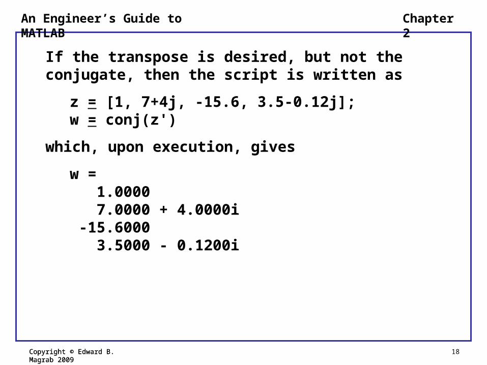
If the transpose is desired, but not the conjugate, then the script is written as
z = [1, 7+4j, -15.6, 3.5-0.12j];w = conj(z')
which, upon execution, gives
w = 1.0000 7.0000 + 4.0000i -15.6000 3.5000 - 0.1200i

Copyright © Edward B. Magrab 2009 19Copyright © Edward B. Magrab 2009
Chapter 2An Engineer’s Guide to MATLAB
Accessing Elements of Vectors – Subscript Notation
Consider the row vector
b = [b1 b2 b3 … bn]
Access to one or more elements of this vector is accomplished using subscript notation in which the subscript refers to the location in the vector as follows:
b(1) b1
…
b(k) bk
...
b(n) bn % or b(end)

Copyright © Edward B. Magrab 2009 20Copyright © Edward B. Magrab 2009
Chapter 2An Engineer’s Guide to MATLAB
Example –
x = [-2, 1, 3, 5, 7, 9, 10];b = x(4)c = x(6)xlast = x(end)
When executed, we obtain
b = 5c = 9xlast = 10

Copyright © Edward B. Magrab 2009 21Copyright © Edward B. Magrab 2009
Chapter 2An Engineer’s Guide to MATLAB
Accessing Elements of Vectors Using Subscript Colon Notation
The subscript colon notation is a shorthand method of accessing a group of elements.
For a vector b with n elements, one can access a group of them using the notation
b(k:d:m)
where 1 k < m n, k and m are positive integers and, in this case, d is a positive integer.
Thus, if one has 10 elements in a vector b, the third through seventh elements are selected by using
b(3:7)

Copyright © Edward B. Magrab 2009 22Copyright © Edward B. Magrab 2009
Chapter 2An Engineer’s Guide to MATLAB
Example –
Consider the following script
z = [-2, 1, 3, 5, 7, 9, 10];z(2) = z(2)/2;z(3:4) = z(3:4)*3-1;z
When executed, we obtain
z = -2.00 0.50 8.00 14.00 7.00 9.00 10.00
Copyright © Edward B. Magrab 2009 23Copyright © Edward B. Magrab 2009
Chapter 2An Engineer’s Guide to MATLAB
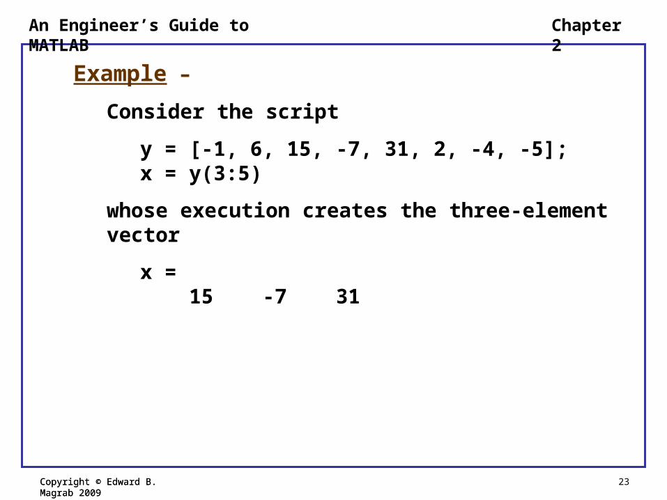
Example –
Consider the script
y = [-1, 6, 15, -7, 31, 2, -4, -5];x = y(3:5)
whose execution creates the three-element vector
x = 15 -7 31

Copyright © Edward B. Magrab 2009 24Copyright © Edward B. Magrab 2009
Chapter 2An Engineer’s Guide to MATLAB
Example –
We shall show that there are several ways to create a vector x that is composed of the first two and the last two elements of a vector y. Thus,
y = [-1, 6, 15, -7, 31, 2, -4, -5];x = [y(1), y(2), y(7), y(8)]
or
y = [-1, 6, 15, -7, 31, 2, -4, -5];index = [1, 2, 7, 8]; % or [1:2, length(y)-1, length(y)] x = y(index)
or more compactly
y = [-1, 6, 15, -7, 31, 2, -4, -5];x = y([1, 2, 7, 8]) % or y([1:2, length(y)-1, length(y)])

Copyright © Edward B. Magrab 2009 25Copyright © Edward B. Magrab 2009
Chapter 2An Engineer’s Guide to MATLAB
Two useful functions: sort and find
sort: Sorts a vector y in ascending order (most negative to most positive) or descending order (most positive to most negative)
[ynew, indx] = sort(y, mode) % mode = 'ascend‘ or 'descend'
where ynew is the vector with the rearranged (sorted) elements of y and indx is a vector containing the original locations of the elements in y.
find: Determines the locations (not the values) of all the elements in a vector (or matrix) that satisfy a user-specified relational and/or logical condition or expression Expr
indxx = find(Expr)

Copyright © Edward B. Magrab 2009 26Copyright © Edward B. Magrab 2009
Chapter 2An Engineer’s Guide to MATLAB
Example –
y = [-1, 6, 15, -7, 31, 2, -4, -5];z = [10, 20, 30, 40, 50, 60, 70, 80];[ynew, indx] = sort(y, 'ascend')znew = z(indx)
when executed, gives
ynew = -7 -5 -4 -1 2 6 15 31indx = 4 8 7 1 6 2 3 5znew = 40 80 70 10 60 20 30 50

Copyright © Edward B. Magrab 2009 27Copyright © Edward B. Magrab 2009
Chapter 2An Engineer’s Guide to MATLAB
Example –
y = [-1, 6, 15, -7, 31, 2, -4, -5];indxx = find(y<=0)s = y(indxx)
Upon execution, we obtain
indxx = 1 4 7 8s = -1 -7 -4 -5

Copyright © Edward B. Magrab 2009 28Copyright © Edward B. Magrab 2009
Chapter 2An Engineer’s Guide to MATLAB
One of the great advantages of MATLAB’s implicit vector and matrix notation is that it provides the user with a compact way of performing a series of operations on an array of values.
Example –
The script
x = linspace(-pi, pi, 10);y = sin(x)
yields the following vector
y = -0.0000 -0.6428 -0.9848 -0.8660 -0.3420 0.3420 0.8660 0.9848 0.6428 0.0000

Copyright © Edward B. Magrab 2009 29Copyright © Edward B. Magrab 2009
Chapter 2An Engineer’s Guide to MATLAB
Minimum and Maximum Values of a Vector: min and max
To find the magnitude of the smallest element xmin and its location locmin in a vector, we use
[xmin, locmin] = min(x)
To find the magnitude of the largest element xmax and its location locmax in a vector, we use
[xmax, locmax] = max(x)

Copyright © Edward B. Magrab 2009 30Copyright © Edward B. Magrab 2009
Chapter 2An Engineer’s Guide to MATLAB
Example –
x = linspace(-pi, pi, 10);y = sin(x);[ymax, kmax] = max(y)[ymin, kmin] = min(y)
Upon execution, we find that
ymax = 0.9848kmax = 8ymin = -0.9848kmin =
3
y = -0.0000 -0.6428 -0.9848 -0.8660 -0.3420 0.3420 0.8660 0.9848 0.6428 0.0000

Copyright © Edward B. Magrab 2009 31Copyright © Edward B. Magrab 2009
Chapter 2An Engineer’s Guide to MATLAB
Example - Analysis of the elements of a vector
Consider 50 equally-spaced points of the following function
We shall
(a) determine the time at which the minimum positive value of f(t) occurs
(b) the average value of its negative values
The script is
( ) sin( ) 0 2f t t t

Copyright © Edward B. Magrab 2009 32Copyright © Edward B. Magrab 2009
Chapter 2An Engineer’s Guide to MATLAB
t = linspace(0, 2*pi, 50);f = sin(t);fAvgNeg = mean(f(find(f<0)))MinValuef = min(f(find(f>0)));tMinValuef = t(find(f==MinValuef))
Upon execution, we find that
fAvgNeg = -0.6237tMinValuef = 3.0775
0 1 2 3 4 5 6-1
-0.5
0
0.5
1
Copyright © Edward B. Magrab 2009 33Copyright © Edward B. Magrab 2009
Chapter 2An Engineer’s Guide to MATLAB
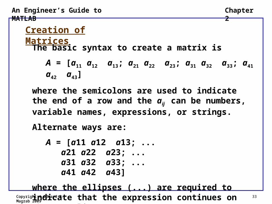
Creation of Matrices
The basic syntax to create a matrix is
A = [a11 a12 a13; a21 a22 a23; a31 a32 a33; a41 a42 a43]
where the semicolons are used to indicate the end of a row and the aij can be numbers, variable names, expressions, or strings.
Alternate ways are:
A = [a11 a12 a13; ... a21 a22 a23; ... a31 a32 a33; ... a41 a42 a43]
where the ellipses (...) are required to indicate that the expression continues on the next line.

Copyright © Edward B. Magrab 2009 34Copyright © Edward B. Magrab 2009
Chapter 2An Engineer’s Guide to MATLAB
For the second alternate way,
One can omit the ellipsis (…) and instead to use the Enter key to indicate the end of a row. In this case, the expression will look like
A = [a11 a12 a13 %<Enter> a21 a22 a23 %<Enter> a31 a32 a33 %<Enter> a41 a42 a43]

Copyright © Edward B. Magrab 2009 35Copyright © Edward B. Magrab 2009
Chapter 2An Engineer’s Guide to MATLAB
For a third alternate way,
Create four separate row vectors, each with the same number of columns, and then combine these vectors to form the matrix as follows
v1 = [ a11 a12 a13];v2 = [ a21 a22 a23];v3 = [ a31 a32 a33];v4 = [ a41 a42 a43]; A = [ v1; v2; v3; v4]
where the semicolons in the first four lines are used to suppress display to the command window.
The order of the matrix is determined by
[r, c] = size(A)

Copyright © Edward B. Magrab 2009 36Copyright © Edward B. Magrab 2009
Chapter 2An Engineer’s Guide to MATLAB
Transpose of a matrix with complex elements
If a matrix has elements that are complex numbers, then taking its transpose also converts the complex quantities to their complex conjugate values.
Consider the following script
Z = [1+2j, 3+4j; 5+6j, 7+9j]W = Z'
the execution of which gives
Z = 1.0000 + 2.0000i 3.0000 + 4.0000i 5.0000 + 6.0000i 7.0000 + 9.0000iW = 1.0000 - 2.0000i 5.0000 - 6.0000i 3.0000 - 4.0000i 7.0000 - 9.0000i

Copyright © Edward B. Magrab 2009 37Copyright © Edward B. Magrab 2009
Chapter 2An Engineer’s Guide to MATLAB
Special Matrices
A matrix of all 1’s
ones(r, c) on(1:r,1:c) = 1 on = ones(2, 5) on = 1 1 1 1 1 1 1 1 1 1
A null matrix
zeros(r, c) zer(1:r,1:c) = 0 zer = zeros(3, 2) zer = 0 0 0 0 0 0

Copyright © Edward B. Magrab 2009 38Copyright © Edward B. Magrab 2009
Chapter 2An Engineer’s Guide to MATLAB
Diagonal matrix –
Create an (nn) diagonal matrix whose diagonal elements are a vector a of length n
diag(a)
a = [4, 9, 1];A = diag(a)A = 4 0 0 0 9 0 0 0 1
Extract the diagonal elements of a square matrix A
diag(A)
Ad = diag([11, 12, 13, 14; … 21, 22, 23, 24; … 31, 32, 33, 34; … 41, 42, 43, 44])Ad = 11 22 33 44

Copyright © Edward B. Magrab 2009 39Copyright © Edward B. Magrab 2009
Chapter 2An Engineer’s Guide to MATLAB
Identity matrix whose size is (nn)
eye(n) A = eye(3)A = 1 0 0 0 1 0 0 0 1

Copyright © Edward B. Magrab 2009 40Copyright © Edward B. Magrab 2009
Chapter 2An Engineer’s Guide to MATLAB
Accessing Matrix Elements
: means all elements of
column 2
: means all elements of
row 2
B = A(1:3,3:5)B = 7.0000 9.0000 11.0000 20.5000 20.7500 21.0000 1.0000 1.0000 1.0000
Matrix created with –
A = [3:2:11; … linspace(20, 21, 5); … ones(1, 5)];
3 5 7 9 11
20.0 20.25 20.5 20.75 21.0
1 1 1 1 1
A
A(1,1)
A(:,2) A(3,4)
A(1:3,3:5)
A(2,:)

Copyright © Edward B. Magrab 2009 41Copyright © Edward B. Magrab 2009
Chapter 2An Engineer’s Guide to MATLAB
In several of the following examples, we shall use
magic(n)
which creates an (nn) matrix in which the sum of the elements in each column and the sum of the elements of each row and the sum of the elements in each diagonal are equal.
For example,
magic(4)
creates
16 2 3 135 11 10 89 7 6 12
4 14 15 1

Copyright © Edward B. Magrab 2009 42Copyright © Edward B. Magrab 2009
Chapter 2An Engineer’s Guide to MATLAB
Example –
We shall set all the diagonal elements of magic(4) to zero; thus
Z = magic(4);Z = Z-diag(diag(Z))
which results in
Z= 0 2 3 13 5 0 10 8 9 7 0 12 4 14 15 0
diag(Z) = 16 11 6 1
diag(diag(Z)) = 16 0 0 0 0 11 0 0 0 0 6 0 0 0 0 1
magic(4) = 16 2 3 135 11 10 89 7 6 124 14 15 1

Copyright © Edward B. Magrab 2009 43Copyright © Edward B. Magrab 2009
Chapter 2An Engineer’s Guide to MATLAB
Example –
We shall replace all the diagonal elements of magic(4) with the value 5; thus,
Z = magic(4);Z = Z-diag(diag(Z))+5*eye(4)
which results in
Z = 5 2 3 13 5 5 10 8 9 7 5 12 4 14 15 5
magic(4) = 16 2 3 135 11 10 89 7 6 124 14 15 1

Copyright © Edward B. Magrab 2009 44Copyright © Edward B. Magrab 2009
Chapter 2An Engineer’s Guide to MATLAB
Use of find with Matrices
For a matrix,
[row, col] = find(Expr)
where row and col are column vectors of the locations in the matrix that satisfied the condition represented by Expr.
Let us find all the elements of magic(3) that are greater than 5. The script is
m = magic(3) [r, c] = find(m > 5);subscr = [r c] % Column augmentation

Copyright © Edward B. Magrab 2009 45Copyright © Edward B. Magrab 2009
Chapter 2An Engineer’s Guide to MATLAB
Upon execution, we obtain
m = 8 1 6 3 5 7 4 9 2subscr = 1 1 3 2 1 3 2 3
Copyright © Edward B. Magrab 2009 46Copyright © Edward B. Magrab 2009
Chapter 2An Engineer’s Guide to MATLAB
which, upon execution, gives
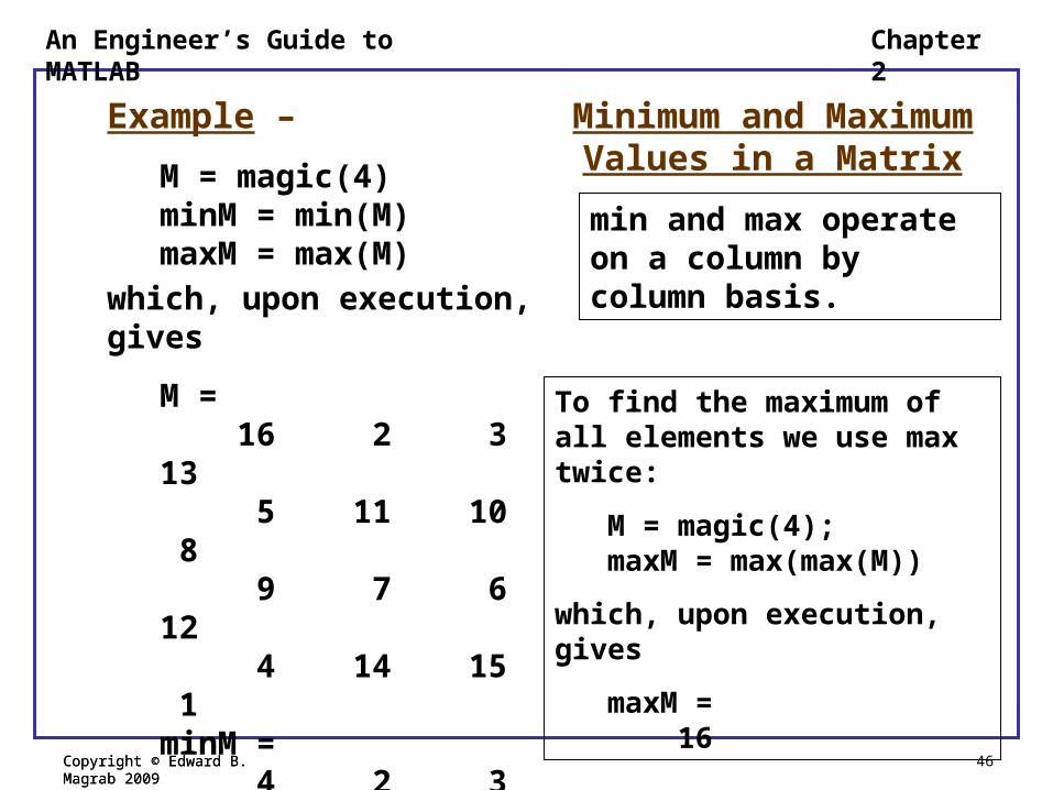
M = 16 2 3 13 5 11 10 8 9 7 6 12 4 14 15 1minM = 4 2 3 1maxM = 16 14 15 13
Example –
M = magic(4)minM = min(M)maxM = max(M)
To find the maximum of all elements we use max twice:
M = magic(4);maxM = max(max(M))
which, upon execution, gives
maxM = 16
Minimum and Maximum Values in a Matrix
min and max operate on a column by column basis.
Copyright © Edward B. Magrab 2009 47Copyright © Edward B. Magrab 2009
Chapter 2An Engineer’s Guide to MATLAB
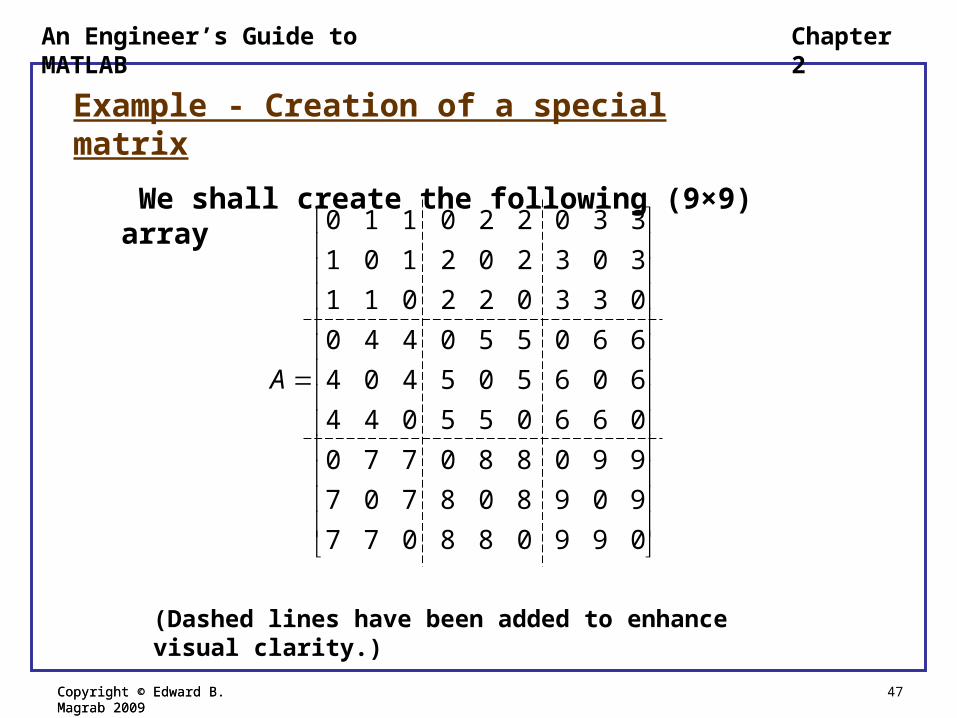
Example - Creation of a special matrix
We shall create the following (9×9) array
(Dashed lines have been added to enhance visual clarity.)
0 1 1 0 2 2 0 3 3
1 0 1 2 0 2 3 0 3
1 1 0 2 2 0 3 3 0
0 4 4 0 5 5 0 6 6
4 0 4 5 0 5 6 0 6
4 4 0 5 5 0 6 6 0
0 7 7 0 8 8 0 9 9
7 0 7 8 0 8 9 0 9
7 7 0 8 8 0 9 9 0
A
Copyright © Edward B. Magrab 2009 48Copyright © Edward B. Magrab 2009
Chapter 2An Engineer’s Guide to MATLAB
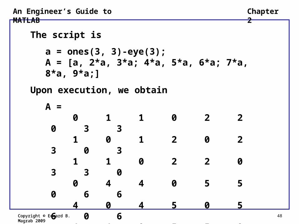
The script is
a = ones(3, 3)-eye(3);A = [a, 2*a, 3*a; 4*a, 5*a, 6*a; 7*a, 8*a, 9*a;]
Upon execution, we obtain
A = 0 1 1 0 2 2 0 3 3 1 0 1 2 0 2 3 0 3 1 1 0 2 2 0 3 3 0 0 4 4 0 5 5 0 6 6 4 0 4 5 0 5 6 0 6 4 4 0 5 5 0 6 6 0 0 7 7 0 8 8 0 9 9 7 0 7 8 0 8 9 0 9 7 7 0 8 8 0 9 9 0

Copyright © Edward B. Magrab 2009 49Copyright © Edward B. Magrab 2009
Chapter 2An Engineer’s Guide to MATLAB
Example - Rearrangement of Sub Matrices of a Matrix
Consider the following (9×9) array
1 2 3 4 5 6 7 8 9
10 11 12 13 14 15 16 17 18
19 20 21 22 23 24 25 26 27
28 29 30 31 32 33 34 35 36
37 38 39 40 41 42 43 44 45
46 47 48 49 50 51 52 53 54
55 56 57 58 59 60 61 62 63
64 65 66 67 68 69 70 71 72
73 74 75 76 77 78 79 80 81
A
1 2
4 3
(Dashed lines have been added to enhance visual clarity.)

Copyright © Edward B. Magrab 2009 50Copyright © Edward B. Magrab 2009
Chapter 2An Engineer’s Guide to MATLAB
For the four (33) sub matrices identified by the circled numbers 1 to 4, we shall perform a series of swaps of these sub matrices to produce the following array
61 62 63 4 5 6 55 56 57
70 71 72 13 14 15 64 65 66
79 80 81 22 23 24 73 74 75
28 29 30 31 32 33 34 35 36
37 38 39 40 41 42 43 44 45
46 47 48 49 50 51 52 53 54
7 8 9 58 59 60 1 2 3
16 17 18 67 68 69 10 11 12
25 26 27 76 77 78 19 20 21
A
3 4
2 1
1 2 3 4 5 6 7 8 9
10 11 12 13 14 15 16 17 18
19 20 21 22 23 24 25 26 27
28 29 30 31 32 33 34 35 36
37 38 39 40 41 42 43 44 45
46 47 48 49 50 51 52 53 54
55 56 57 58 59 60 61 62 63
64 65 66 67 68 69 70 71 72
73 74 75 76 77 78 79 80 81
A
1 2
4 3

Copyright © Edward B. Magrab 2009 51Copyright © Edward B. Magrab 2009
Chapter 2An Engineer’s Guide to MATLAB
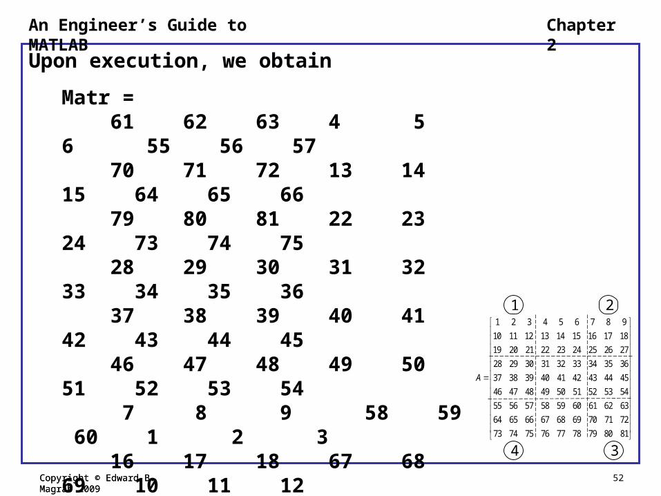
The script is
Matr = [1:9; 10:18; 19:27; 28:36; 37:45; ... 46:54; 55:63; 64:72; 73:81];
Temp1 = Matr(1:3, 1:3);Matr(1:3, 1:3) = Matr(7:9, 7:9);Matr(7:9, 7:9) = Temp1;Temp1 = Matr(1:3, 7:9);Matr(1:3, 7:9) = Matr(7:9, 1:3);Matr(7:9, 1:3) = Temp1;Matr
Copyright © Edward B. Magrab 2009 52Copyright © Edward B. Magrab 2009
Chapter 2An Engineer’s Guide to MATLAB
Upon execution, we obtain
Matr = 61 62 63 4 5 6 55 56 57 70 71 72 13 14 15 64 65 66 79 80 81 22 23 24 73 74 75 28 29 30 31 32 33 34 35 36 37 38 39 40 41 42 43 44 45 46 47 48 49 50 51 52 53 54 7 8 9 58 59 60 1 2 3 16 17 18 67 68 69 10 11 12 25 26 27 76 77 78 19 20 21 1 2 3 4 5 6 7 8 9
10 11 12 13 14 15 16 17 18
19 20 21 22 23 24 25 26 27
28 29 30 31 32 33 34 35 36
37 38 39 40 41 42 43 44 45
46 47 48 49 50 51 52 53 54
55 56 57 58 59 60 61 62 63
64 65 66 67 68 69 70 71 72
73 74 75 76 77 78 79 80 81
A
1 2
4 3

Copyright © Edward B. Magrab 2009 53Copyright © Edward B. Magrab 2009
Chapter 2An Engineer’s Guide to MATLAB
Manipulation of Arrays
Two functions that create matrices by replicating a specified number of times either a scalar, a column or row vector, or a matrix are
repmat
and
meshgrid
which uses repmat. The general form of repmat is
repmat(x, r, c)
where x is either a scalar, vector, or matrix, r is the total number of rows of x that will be replicated, and c is the total number of columns of x will be replicated.

Copyright © Edward B. Magrab 2009 54Copyright © Edward B. Magrab 2009
Chapter 2An Engineer’s Guide to MATLAB
Example –
We shall produce the following matrix three ways
W = 45.7200 45.7200 45.7200 45.7200 45.7200 45.7200 45.7200 45.7200 45.7200
Thus,
W = repmat(45.72, 3, 3) % Function
or
W = [45.72, 45.72, 45.72; … % Hard code 45.72, 45.72, 45.72; … 45.72, 45.72, 45.72]
or
W(1:3,1:3) = 45.72 % Subscript colon notation

Copyright © Edward B. Magrab 2009 55Copyright © Edward B. Magrab 2009
Chapter 2An Engineer’s Guide to MATLAB
Example –
Consider the vector
s = [a1 a2 a3 a4]
The expression
V = repmat(s, 3, 1)
creates the numerical equivalent of the matrix
1 2 3 4
1 2 3 4
1 2 3 4
=
a a a a
V a a a a
a a a aReplicated
row

Copyright © Edward B. Magrab 2009 56Copyright © Edward B. Magrab 2009
Chapter 2An Engineer’s Guide to MATLAB
whereas
repmat(s, 3, 2)
creates the numerical equivalent of the matrix
1 2 3 4 1 2 3 4
1 2 3 4 1 2 3 4
1 2 3 4 1 2 3 4
=
a a a a a a a a
V a a a a a a a a
a a a a a a a a
Replicated ‘column’
Replicated 1st row
Copyright © Edward B. Magrab 2009 57Copyright © Edward B. Magrab 2009
Chapter 2An Engineer’s Guide to MATLAB
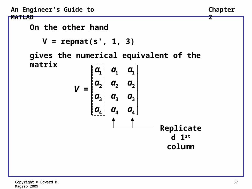
On the other hand
V = repmat(s', 1, 3)
gives the numerical equivalent of the matrix
1 1 1
2 2 2
3 3 3
4 4 4
=
a a a
a a aV
a a a
a a a
Replicated 1st column

Copyright © Edward B. Magrab 2009 58Copyright © Edward B. Magrab 2009
Chapter 2An Engineer’s Guide to MATLAB
and
V = repmat(s', 2, 3)
gives the numerical equivalent of the matrix
1 1 1
2 2 2
3 3 3
4 4 4
1 1 1
2 2 2
3 3 3
4 4 4
=
a a a
a a a
a a a
a a aV
a a a
a a a
a a a
a a a

Copyright © Edward B. Magrab 2009 59Copyright © Edward B. Magrab 2009
Chapter 2An Engineer’s Guide to MATLAB
meshgrid
If we have two row vectors s and t, then
[U, V] = meshgrid(s, t)
gives the same result as that produced by the two commands
U = repmat(s, length(t), 1)
V = repmat(t', 1, length(s)) % Notice transpose
In either case, U and V are each matrices of order
(length(t)length(s))

Copyright © Edward B. Magrab 2009 60Copyright © Edward B. Magrab 2009
Chapter 2An Engineer’s Guide to MATLAB
Example –
If
s = [s1 s2 s3 s4] % (1×4) t = [t1 t2 t3] % (1×3)
then
[U, V] = meshgrid(s, t) % Sizes of U and V are (3×4)
produces the numerical equivalent of two (34) matrices
1 2 3 4
1 2 3 4
1 2 3 4
=
s s s s
U s s s s
s s s s
1 1 1 1
2 2 2 2
3 3 3 3
=
t t t t
V t t t t
t t t t

Copyright © Edward B. Magrab 2009 61Copyright © Edward B. Magrab 2009
Chapter 2An Engineer’s Guide to MATLAB
Example –
u = [1, 2, 3, 4];v = [5, 6, 7];[U, V] = meshgrid(u, v)
Upon execution, we obtain
U = 1 2 3 4 1 2 3 4 1 2 3 4V = 5 5 5 5 6 6 6 6 7 7 7 7
However, u = [1, 2, 3, 4];v = [5, 6, 7];[V, U] = meshgrid(v, u)
gives
V = 5 6 7 5 6 7 5 6 7 5 6 7U = 1 1 1 2 2 2 3 3 3 4 4 4

Copyright © Edward B. Magrab 2009 62Copyright © Edward B. Magrab 2009
Chapter 2An Engineer’s Guide to MATLAB
There are two matrix manipulation functions that are useful in certain applications –
fliplr(A)
which flips the columns and
flipud(A)
which flips the rows.
Consider the (25) matrix
( )
11 12 13 14 15
21 22 23 24 25
= 2×5a a a a a
Aa a a a a
which is created with the statement
A = [a11 a12 a13 a14 a15; a21 a22 a23 a24 a25]

Copyright © Edward B. Magrab 2009 63Copyright © Edward B. Magrab 2009
Chapter 2An Engineer’s Guide to MATLAB
Then
15 14 13 12 11
25 24 23 22 21
21 22 23 24 25
11 12 13 14 15
( ) = (2×5)
( ) = (2×5)
a a a a aA
a a a a a
a a a a aA
a a a a a
fliplr
flipud
and
( ( ))
25 24 23 22 21
15 14 13 12 11
(2×5)a a a a a
Aa a a a a
flipud fliplr
These results are obtained with the colon notation. For example,
C = fliplr(A)
produces the same results as
C = A(:,length(A):-1:1)
( )
11 12 13 14 15
21 22 23 24 25
= 2×5a a a a a
Aa a a a a

Copyright © Edward B. Magrab 2009 64Copyright © Edward B. Magrab 2009
Chapter 2An Engineer’s Guide to MATLAB
Clarification of Notation –
Consider the following two (25) matrices A and B
11 12 13 14 15 11 12 13 14 15
21 22 23 24 25 21 22 23 24 25
a a a a a b b b b bA B
a a a a a b b b b b
Addition or subtraction: C = A B
11 11 12 12 13 13 14 14 15 15
21 21 22 22 23 23 24 24 25 25
± ± ± ± ±(2×5)
± ± ± ± ±
a b a b a b a b a bC
a b a b a b a b a b

Copyright © Edward B. Magrab 2009 65Copyright © Edward B. Magrab 2009
Chapter 2An Engineer’s Guide to MATLAB
Column augmentation: C = [A, B]
11 12 13 14 15 11 12 13 14 15
21 22 23 24 25 21 22 23 24 25
(2×10)a a a a a b b b b b
Ca a a a a b b b b b
Row augmentation: C = [A; B]
11 12 13 14 15
21 22 23 24 25
11 12 13 14 15
21 22 23 24 25
(4×5)
a a a a a
a a a a aC
b b b b b
b b b b b
Copyright © Edward B. Magrab 2009 66Copyright © Edward B. Magrab 2009
Chapter 2An Engineer’s Guide to MATLAB
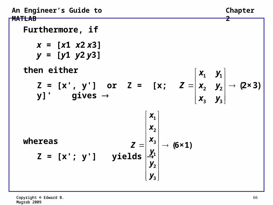
Furthermore, if
x = [x1 x2 x3]y = [y1 y2 y3]
then either
Z = [x', y'] or Z = [x; y]' gives
whereas
Z = [x'; y'] yields
1 1
2 2
3 3
(2× 3)
x y
Z x y
x y
1
2
3
1
2
3
(6×1)
x
x
xZ
y
y
y

Copyright © Edward B. Magrab 2009 67Copyright © Edward B. Magrab 2009
Chapter 2An Engineer’s Guide to MATLAB
We illustrate these results with the following two vectors: a = [1, 2, 3] and b = [4, 5, 6]. The script is
x = [1, 2, 3];y = [4, 5, 6];Z1= [x', y']Z2= [x; y]'Z3= [x'; y']
Z1 = 1 4 2 5 3 6
Z3 = 1 2 3 4 5 6
Z2 = 1 4 2 5 3 6

Copyright © Edward B. Magrab 2009 68Copyright © Edward B. Magrab 2009
Chapter 2An Engineer’s Guide to MATLAB
Dot Operations
A means of performing, on matrices of the same order, arithmetic operations on an element-by-element basis.
Consider the following (34) matrices
11 12 13 14
21 22 23 24
31 32 33 34
x x x x
X x x x x
x x x x
11 12 13 14
21 22 23 24
31 32 33 34
m m m m
M m m m m
m m m m

Copyright © Edward B. Magrab 2009 69Copyright © Edward B. Magrab 2009
Chapter 2An Engineer’s Guide to MATLAB
11 11 12 12 13 13 14 14
21 21 22 22 23 23 24 24
31 31 32 32 33 33 34 34
* * * *
* * * *
* * * *m
x m x m x m x m
Z X.* M x m x m x m x m
x m x m x m x m
Then, the dot multiplication of X and M is
The dot division of X by M is
11 11 12 12 13 13 14 14
21 21 22 22 23 23 24 24
31 31 32 32 33 33 34 34
/m /m /m /m
/m /m /m /m
/m /m /m /md
x x x x
Z X./M x x x x
x x x x

Copyright © Edward B. Magrab 2009 70Copyright © Edward B. Magrab 2009
Chapter 2An Engineer’s Guide to MATLAB
11 11 12 12 13 13 14 14
21 21 22 22 23 23 24 24
31 31 32 32 33 33 34 34
^ ^ ^ ^
^ ^ ^ ^
^ ^ ^ ^e
x m x m x m x m
Z X.^ M x m x m x m x m
x m x m x m x m
The dot exponentiation of X and M is

Copyright © Edward B. Magrab 2009 71Copyright © Edward B. Magrab 2009
Chapter 2An Engineer’s Guide to MATLAB
Use of Dot Operations
Let a, b, c, d, and g each be a (32) matrix, and consider the expression
2
tand
bZ = a - g
c
Then the MATLAB expression is
Z = (tan(a)-g.*(b./c).^d).^2;
which is equivalent to
11 11 11 11 11 12 12 12 12 12
21 21 21 21 21 22 22 22 22 22
31 31 31 31 31 32 32 32 32 32
(tan( ) - * ( / )^ )^ 2 (tan( ) - * ( / )^ )^ 2
(tan( ) - * ( / )^ )^ 2 (tan( ) - * ( / )^ )^ 2
(tan( ) - * ( / )^ )^ 2 (tan( ) - * ( / )^ )^ 2
a g b c d a g b c d
Z a g b c d a g b c d
a g b c d a g b c d

Copyright © Edward B. Magrab 2009 72Copyright © Edward B. Magrab 2009
Chapter 2An Engineer’s Guide to MATLAB
Example –
Evaluate
1 1 1
1
sin( )a t b t cv e
t c
for 6 equally-spaced values of t in the interval 0 t 1 when a1 = 0.2, b1 = 0.9, and c1 = /6. The script is
a1 = 0.2; b1 = 0.9; c1 = pi/6;t = linspace(0, 1, 6);v = exp(-a1*t).*sin(b1*t+c1)./(t+c1)
Upon execution, we obtain
v = 0.9549 0.8590 0.7726 0.6900 0.6097 0.5316

Copyright © Edward B. Magrab 2009 73Copyright © Edward B. Magrab 2009
Chapter 2An Engineer’s Guide to MATLAB
Example –
Create the elements of an (N×N) matrix H when each element is given by
1 , 1, 2,...
1mnh m n Nm n
The script to generate this array for N = 4 is
N = 4;mm = 1:N; nn = mm;[n, m] = meshgrid(nn, mm)h = 1./(m+n-1)
Upon execution, we get h = 1.0000 0.5000 0.3333 0.2500 0.5000 0.3333 0.2500 0.2000 0.3333 0.2500 0.2000 0.1667 0.2500 0.2000 0.1667 0.1429

Copyright © Edward B. Magrab 2009 74Copyright © Edward B. Magrab 2009
Chapter 2An Engineer’s Guide to MATLAB
We return to meshgrid and again consider the two vectors s = [s1 s2 s3 s4] and t = [t1 t2 t3]. Using the MATLAB expression
[U, V] = meshgrid(s, t) % U and V are (3×4) matrices
we obtained the matrices
If we perform the dot multiplication
Z = U.*V
then the execution of the program
1 2 3 4
1 2 3 4
1 2 3 4
=
s s s s
U s s s s
s s s s
1 1 1 1
2 2 2 2
3 3 3 3
=
t t t t
V t t t t
t t t t
and
Copyright © Edward B. Magrab 2009 75Copyright © Edward B. Magrab 2009
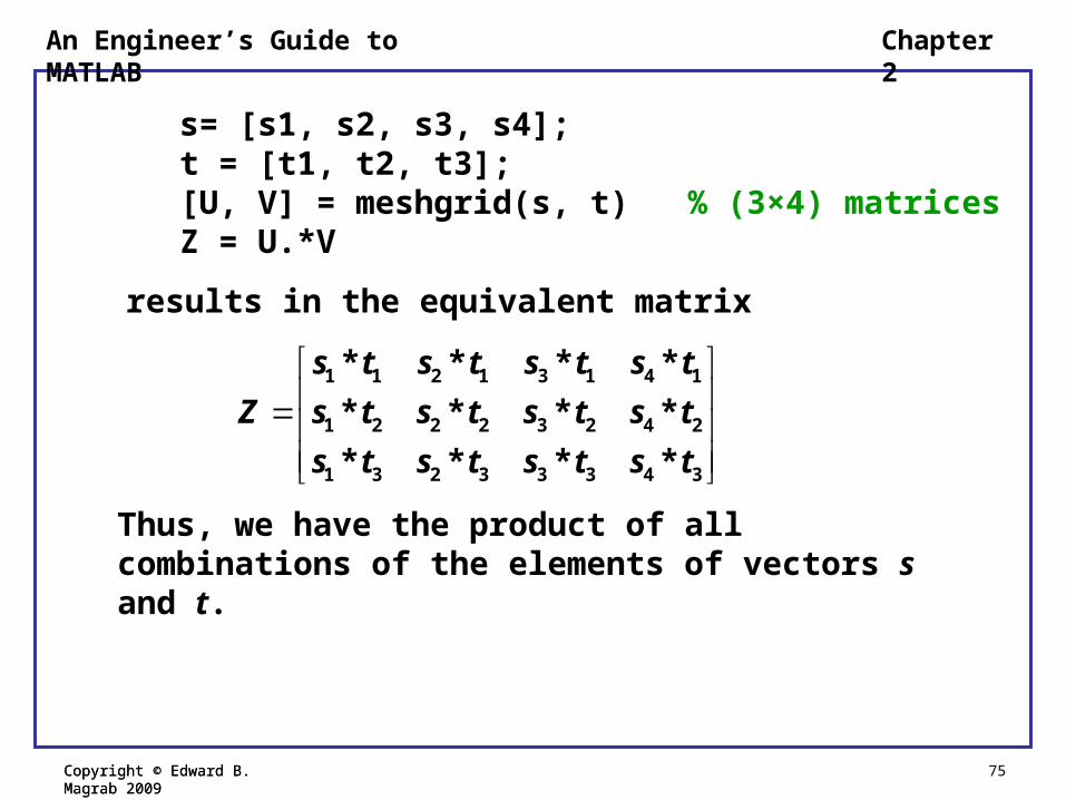
Chapter 2An Engineer’s Guide to MATLAB
s= [s1, s2, s3, s4];t = [t1, t2, t3];[U, V] = meshgrid(s, t) % (3×4) matricesZ = U.*V
results in the equivalent matrix
1 1 2 1 3 1 4 1
1 2 2 2 3 2 4 2
1 3 2 3 3 3 4 3
* * * *
* * * *
* * * *
s t s t s t s t
Z s t s t s t s t
s t s t s t s t
Thus, we have the product of all combinations of the elements of vectors s and t.

Copyright © Edward B. Magrab 2009 76Copyright © Edward B. Magrab 2009
Chapter 2An Engineer’s Guide to MATLAB
Summation and Cumulative Summation Functions
sum: When v = [v1, v2, …, vn], then
( )
1
( )v
kk
S v vlength
sum
where S a scalar.
If Z is a (34) matrix with elements zij, then
( )
3 3 3 3
1 2 3 4=1 =1 =1 =1
, , , (1×4)n n n nn n n n
S Z z z z zsum
To sum all the elements in an array, we use
( ( )) 3 3 3 3 4 3
1 2 3 4=1 =1 =1 =1 =1 =1
+ + + (1×1)n n n n nin n n n i n
S Z z z z z zsum sum

Copyright © Edward B. Magrab 2009 77Copyright © Edward B. Magrab 2009
Chapter 2An Engineer’s Guide to MATLAB
Example –
Evaluate
4
=1
m
m
z m
Thus,
m = 1:4;z = sum(m.^m)
which, when executed, gives
z = 288

Copyright © Edward B. Magrab 2009 78Copyright © Edward B. Magrab 2009
Chapter 2An Engineer’s Guide to MATLAB
cumsum: For a vector v composed of n elements vj, cumsum creates another vector of length n whose elements are
( )
1 2
=1 =1 =1
, , ... (1× )n
k k kk k k
y v v v v ncumsum
If W is (mn) matrix composed of elements wjk, then
( ) ( )
1 1 1
1 2=1 k =1 k =1
2 2
1 2=1 k =1
1=1 k =1
...
... ...
k k knk
k kk
m m
k knk
w w w
w wY W m×n
w w
cumsum

Copyright © Edward B. Magrab 2009 79Copyright © Edward B. Magrab 2009
Chapter 2An Engineer’s Guide to MATLAB
Example –
Consider the convergence of the series
N N=10
2=1
1
n
Sn
Thus,
S = cumsum(1./(1:10).^2)
which, upon execution, gives
S = 1.0000 1.2500 1.3611 1.4236 1.4636 1.4914 1.5118 1.5274 1.5398 1.5498

Copyright © Edward B. Magrab 2009 80Copyright © Edward B. Magrab 2009
Chapter 2An Engineer’s Guide to MATLAB
Example –
We shall evaluate the following series expression for the hyperbolic secant for N = 305 and for five equally spaced values of x from 0 x 2 and compare the results to the exact values.
4
( -1)/2
2 2=1,3,5
(-1)sech
+ 4
nN
n
nx
nπ xThus,
nn = 1:2:305; % (1153) xx = linspace(0, 2, 5); % (15)[x, n] = meshgrid(xx, nn); % (1535)s = 4*pi*sum(n.*(-1).^((n-1)/2)./…
((pi*n).^2+4*x.^2)); % (15)se = sech(xx); % (15)compare = [xx ' s' se' (100*(s-se)./se)'] % (52)

Copyright © Edward B. Magrab 2009 81Copyright © Edward B. Magrab 2009
Chapter 2An Engineer’s Guide to MATLAB
which, upon execution, gives
compare = 0.0000 1.0021 1.0000 0.2080 0.5000 0.8889 0.8868 0.2346 1.0000 0.6501 0.6481 0.3210 1.5000 0.4272 0.4251 0.4894
2.0000 0.2679 0.2658 0.7827 x approx sech(x) % error

Copyright © Edward B. Magrab 2009 82Copyright © Edward B. Magrab 2009
Chapter 2An Engineer’s Guide to MATLAB
Mathematical Operations with Matrices
Addition and Subtraction
If we have two matrices A and B, each of the order (mn), then
11 11 12 12 1n 1n
21 21 22 22
m1 m1 mn mn
± ± ... ±
± ±( × )
... ...
± ±
a b a b a b
a b a bA± B m n
a b a b
The MATLAB expression for matrix addition or subtraction is
W = A + B or W = A – B

Copyright © Edward B. Magrab 2009 83Copyright © Edward B. Magrab 2009
Chapter 2An Engineer’s Guide to MATLAB
Multiplication
If we have an (mk) matrix A and a (kn) matrix B, then
11 12 1
21 22
1
( )
n
m mn
c c c
c cC AB m n
c c
where
1
k
lp lj jpj
c a b
For the conditions stated, the MATLAB expression for matrix multiplication is
W = A*B

Copyright © Edward B. Magrab 2009 84Copyright © Edward B. Magrab 2009
Chapter 2An Engineer’s Guide to MATLAB
Note: The product of two matrices is defined only when the adjacent integers of their respective orders are equal; k in this case. In other words,
(mk)(kn) (mn)
where the notation indicates that we have summed the k terms.
1
k
lp lj jpj
c a b
Matrix Transpose
It can be shown that if C = AB, then its transpose is ( )C AB B A
If A is an identity matrix (A = I) and m = n, then
C IB BI B

Copyright © Edward B. Magrab 2009 85Copyright © Edward B. Magrab 2009
Chapter 2An Engineer’s Guide to MATLAB
Example –
We shall multiply the following two matrices and show numerically that the transpose can be obtained either of the two ways indicated previously.
11 1211 12 13
21 2221 22 23
31 32
A B
The script is
A = [11, 12, 13; 21, 22, 23];B = [11, 12; 21, 22; 31, 32];C = A*BCtran1 = C'Ctran2 = B'*A'

Copyright © Edward B. Magrab 2009 86Copyright © Edward B. Magrab 2009
Chapter 2An Engineer’s Guide to MATLAB
Upon execution, we obtain
C = 776 812 1406 1472Ctran1 = 776 1406 812 1472Ctran2 = 776 1406 812 1472
A = [11, 12, 13; 21, 22, 23];B = [11, 12; 21, 22; 31, 32];C = A*BCtran1 = C'Ctran2 = B'*A'
Copyright © Edward B. Magrab 2009 87Copyright © Edward B. Magrab 2009
Chapter 2An Engineer’s Guide to MATLAB
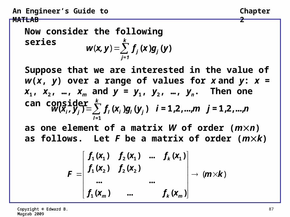
Now consider the following series
( ) ( ) ( )k
j jj=1
w x, y f x g y
Suppose that we are interested in the value of w(x, y) over a range of values for x and y: x = x1, x2, …, xm and y = y1, y2, …, yn. Then one can consider
=1
( ) ( ) ( ) = 1,2, ..., = 1,2, ...,k
i j l i l jl
w x , y f x g y i m j n
as one element of a matrix W of order (mn) as follows. Let F be a matrix of order (mk)
( )
1 1 2 1 1
1 2 2 2
1
( ) ( ) ... ( )
( ) ( )
... ...
( ) ... ( )
k
m k m
f x f x f x
f x f xF m k
f x f x

Copyright © Edward B. Magrab 2009 88Copyright © Edward B. Magrab 2009
Chapter 2An Engineer’s Guide to MATLAB
and G be a matrix of order (kn)
( )
1 1 1 2 1
2 1 2 2
1
( ) ( ) ... ( )
( ) ( ) ...
... ...
( ) ... ( )
n
k k n
g y g y g y
g y g yG k n
g y g y
then
11 12 1
21 22
1
...
...( )
... ...
...
n
m mn
w w w
w wW FG m n
w w
where
1
( , ) ( ) ( )k
ij i j l i l jl
w w x y f x g y

Copyright © Edward B. Magrab 2009 89Copyright © Edward B. Magrab 2009
Chapter 2An Engineer’s Guide to MATLAB
We now consider three special cases of this general matrix multiplication:
1. The product of a row and a column vector
2. The product of a column and a row vector
3. The product of a row vector and a matrix
Thus, matrix multiplication performs the summation of the series at each combination of values for x and y.

Copyright © Edward B. Magrab 2009 90Copyright © Edward B. Magrab 2009
Chapter 2An Engineer’s Guide to MATLAB
Product of a Row Vector and Column Vector
Let a be the row vector
a = [a1 a2 … ak] (1k)
and b be the column vector
b = [b1 b2 … bk] (k1)
Then the product d = ab is the scalar
)
1
11 2
=1 =1
... = (1×1...
k k
k j j j jj j
k
b
bd ab a a a a b a b
b
(1k)(k1)
l =1 and p = 1
11 12 1
21 22
1
1
n
m mn
k
lp lj jpj
c c c
c cC AB
c c
c a b

Copyright © Edward B. Magrab 2009 91Copyright © Edward B. Magrab 2009
Chapter 2An Engineer’s Guide to MATLAB
This is called the dot product of two vectors.
The MATLAB notation for this operation is either
d = a*b
or
d = dot(a, b)

Copyright © Edward B. Magrab 2009 92Copyright © Edward B. Magrab 2009
Chapter 2An Engineer’s Guide to MATLAB
Product of a Column and Row Vector
Let a be an (m1) column vector and b a (1n) row vector. Then the product H = ba is
( )
1 1 1 1 2 1
2 2 1 2 21 2
1
...
......
... ... ...
...
n
n
m m m n
a a b a b a b
a a b a bH ba b b b m n
a a b a b
The elements of H, which are hij = biaj, are the individual products of all the combinations of the elements of b and a.
1
k
lp lj jpj
c a b
l = 1, 2, …, mp = 1, 2, …, n

Copyright © Edward B. Magrab 2009 93Copyright © Edward B. Magrab 2009
Chapter 2An Engineer’s Guide to MATLAB
Example - Polar to Cartesian Coordinates
Consider a vector of radial values
r = [r1 r2 … rm]
and a vector of angular values
= [1 2 … n]
then
*
1
21 2
1 1 1 2 1
2 1 2 2
1
cos( ) cos cos ... cos...
cos cos ... cos
cos cos
... ...
cos ... cos
n
m
n
m m n
r
rX r θ θ θ θ
r
r θ r θ r θ
r θ r θ
r θ r θ
r
y = rsin
x = rcos x
y

Copyright © Edward B. Magrab 2009 94Copyright © Edward B. Magrab 2009
Chapter 2An Engineer’s Guide to MATLAB
and
*
1
21 2
1 1 1 2 1
2 1 2 2
1
sin( ) sin sin ... sin...
sin sin ... sin
sin sin
... ...
sin ... sin
n
m
n
m m n
r
rY r θ θ θ θ
r
r θ r θ r θ
r θ r θ
r θ r θ
A typical MATLAB program would look like
r = [0:0.05:1]'; % (211)phi = 0:pi/20:2*pi; % (141)x = r*cos(phi); % (2141)y = r*sin(phi); % (2141)

Copyright © Edward B. Magrab 2009 95Copyright © Edward B. Magrab 2009
Chapter 2An Engineer’s Guide to MATLAB
Product of a Row Vector and a Matrix
Let B be an (mn) matrix and a a (1m) row vector. Then, the product g = aB is
( )
11 12 1
21 221 2
1
1 2=1 j=1 j=1
...
...... ...
...
... 1
n
m
m mn
m m m
j j j j j jnj
b b b
b bg aB a a a
b b
a b a b a b n
1
k
lp lj jpj
c a b
l = 1p = 1, 2, …, n

Copyright © Edward B. Magrab 2009 96Copyright © Edward B. Magrab 2009
Chapter 2An Engineer’s Guide to MATLAB
( ) =1
( )m
k kk
r x p h x
Now consider the series
Suppose that we are interested in the value of r(x) over a range of values x1, x2, …, xn. Then
is one element of a vector r of order (1n) as follows.
Let p be a vector of order (1m) with elements pk and V be the (mn) matrix
( )
1 1 1 2 1
2 1 2 2
1
( ) ( ) ... ( )
( ) ( )
... ...
( ) ( )
n
m m n
h x h x h x
h x h xV m n
h x h x
( ) =1
( ) = 1,2, ...,m
i k k ik
r x p h x i n

Copyright © Edward B. Magrab 2009 97Copyright © Edward B. Magrab 2009
Chapter 2An Engineer’s Guide to MATLAB
Then, r = pV gives
( ) 1 2
=1 =1 =1
( ) ( ) ... ( ) 1m m m
k k k k k k nk k k
r pV p h x p h x p h x n

Copyright © Edward B. Magrab 2009 98Copyright © Edward B. Magrab 2009
Chapter 2An Engineer’s Guide to MATLAB
Example - Summation of a Fourier Series
The Fourier series representation of a rectangular pulse of duration d and period T is given by
( )
=1
sin1 + 2 cos(2 )
K
k
kπd/Tdf πk
T kπd/T
where = t/T. Let us sum 150 terms of f() (K = 150) and plot it from 1/2 ≤ ≤ 1/2 when d/T = 0.25.
We see that
( ) ( )
( ) ( )
sin
cos(2 )
i
k
k i k i
r x f
kπd/Tp
kπd/T
h x h τ πk
( ) =1
( ) = 1,2, ...,m
i k k ik
r x p h x i n

Copyright © Edward B. Magrab 2009 99Copyright © Edward B. Magrab 2009
Chapter 2An Engineer’s Guide to MATLAB
The program is
k = 1:150; % (1150)tau = linspace(-0.5, 0.5, 100); % (1100)sk = sin(pi*k/4)./(pi*k/4); % (1150)cntau = cos(2*pi*k'*tau); % (150100)f = 0.25*(1+2*sk*cntau); % (1150) (150100) (1100)plot(tau, f)

Copyright © Edward B. Magrab 2009 100Copyright © Edward B. Magrab 2009
Chapter 2An Engineer’s Guide to MATLAB
Example -
31
1 cos( )( , ) 4 sin( )
Nn
n
nu e n
n
Assume that the length of is Nx and that the length of is Ne. Then, we note that
1 cos
sin3
(1 ) (1 )(1 ) (1 )[Not permissible](1 ) [Not permissible]
ex
n ne nn N NN N
N

Copyright © Edward B. Magrab 2009 101Copyright © Edward B. Magrab 2009
Chapter 2An Engineer’s Guide to MATLAB
1 cos
sin3
( 1)(1 )( 1)(1 )( ) (1 ) ( )
( )
eex
x
x
n ne nn N NN N
N NN N N
N N
In order to have the matrices compatible for multiplication, we take the transpose of vector n
1 cos
sin3
( )( )
[dot multiplication]
e
x
n ne nn N N
N N
From meshgrid(, f(n))

Copyright © Edward B. Magrab 2009 102Copyright © Edward B. Magrab 2009
Chapter 2An Engineer’s Guide to MATLAB
1 cos
sin ( )3
( )( ) ( )
e
x x
n ne n N Nx en N N
N N N N
Now we take the transpose and perform matrix multiplication
From the matrix multiplication of these two expressions, we are summing over n, which is what we set out to do.

Copyright © Edward B. Magrab 2009 103Copyright © Edward B. Magrab 2009
Chapter 2An Engineer’s Guide to MATLAB
n = (1:25)*pi; % (125)eta = 0:0.025:1; % (141)xi = 0:0.05:0.7; % (115)[X1, temp1] = meshgrid(xi, (1-cos(n))./n.^3); % (2515)temp2 = exp(-n'*xi); % (2515)Rnx = temp1.*temp2; % (2515)temp3 = sin(n'*eta); % (2541)u = 4*Rnx'*temp3; % (1541)mesh(eta, xi, u)
00.2
0.40.6
0.8
1
0
0.2
0.4
0.6
0.80
0.05
0.1
0.15
0.2
0.25
0.3
0.35

Copyright © Edward B. Magrab 2009 104Copyright © Edward B. Magrab 2009
Chapter 2An Engineer’s Guide to MATLAB
Determinants
A determinant of an array A of order (nn) is represented symbolically as
11 12 1
21 22
1
...
...
... ...
...
n
n nn
a a a
a aA
a a
For n = 2:
For n = 3:
11 22 12 21A a a a a
11 22 33 12 23 31 13 21 32 13 22 31
11 23 32 12 21 33
+ +
A a a a a a a a a a a a a
a a a a a a
Copyright © Edward B. Magrab 2009 105Copyright © Edward B. Magrab 2009
Chapter 2An Engineer’s Guide to MATLAB
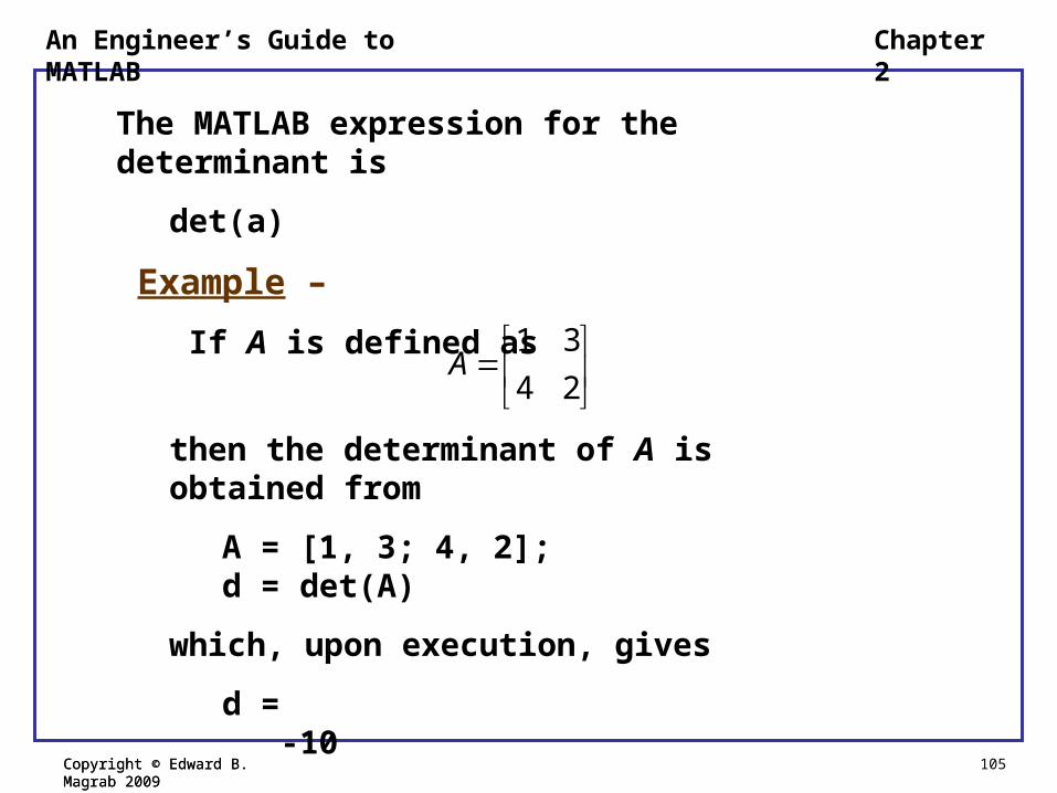
The MATLAB expression for the determinant is
det(a)
Example –
If A is defined as 1 3
4 2A
then the determinant of A is obtained from
A = [1, 3; 4, 2];d = det(A)
which, upon execution, gives
d = -10

Copyright © Edward B. Magrab 2009 106Copyright © Edward B. Magrab 2009
Chapter 2An Engineer’s Guide to MATLAB
A class of problems, called eigenvalue problems, results in a determinant of the form
0A λB
where A and B are (nn) matrices and j, j = 1, 2, , …, n are the roots (called eigenvalues) of this equation.
One form of the MATLAB expression to obtain is
lambda = eig(A, B)
Copyright © Edward B. Magrab 2009 107Copyright © Edward B. Magrab 2009
Chapter 2An Engineer’s Guide to MATLAB
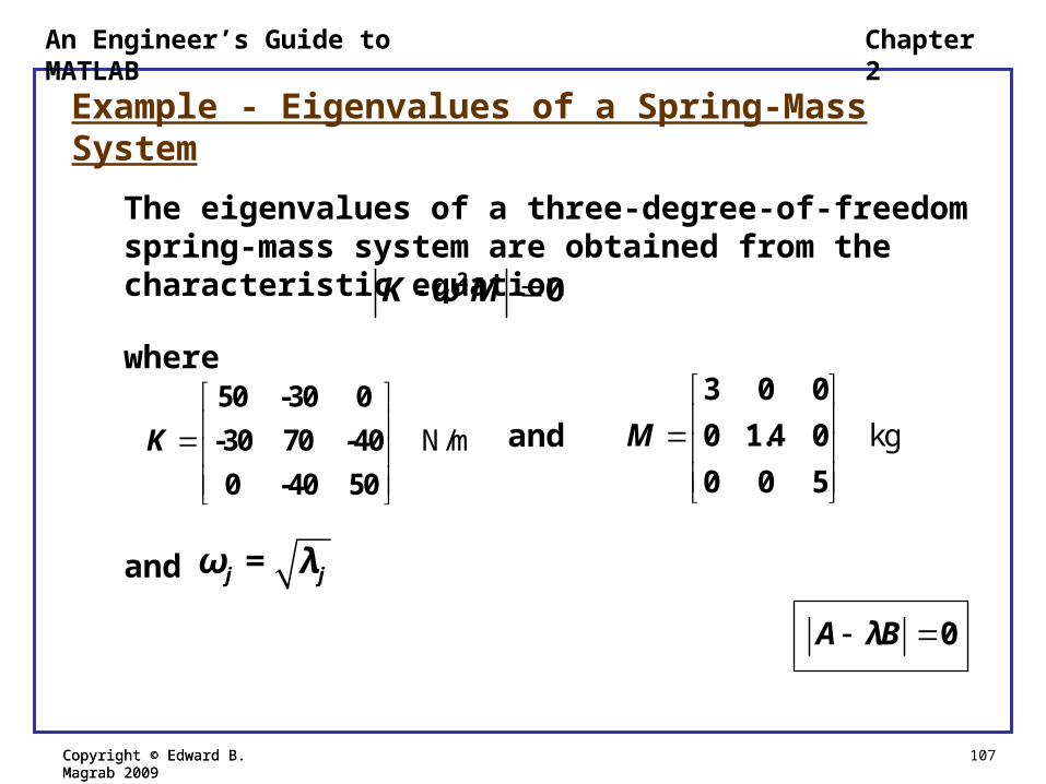
Example - Eigenvalues of a Spring-Mass System
The eigenvalues of a three-degree-of-freedom spring-mass system are obtained from the characteristic equation
2 0K - ω M
where
N/m
50 -30 0
-30 70 -40
0 -40 50
K kg
3 0 0
0 1.4 0
0 0 5
Mand
j jω = λand
0A λB

Copyright © Edward B. Magrab 2009 108Copyright © Edward B. Magrab 2009
Chapter 2An Engineer’s Guide to MATLAB
The program is
K = [50, -30, 0; -30, 70, -40; 0, -40, 50];M = diag([3, 1.4, 5]);w = sqrt(eig(K, M))
which, upon execution, gives
w = 1.6734 3.7772 7.7201
% rad/s
50 -30 0
-30 70 -40
0 -40 50
K
3 0 0
0 1.4 0
0 0 5
M
Copyright © Edward B. Magrab 2009 109Copyright © Edward B. Magrab 2009
Chapter 2An Engineer’s Guide to MATLAB
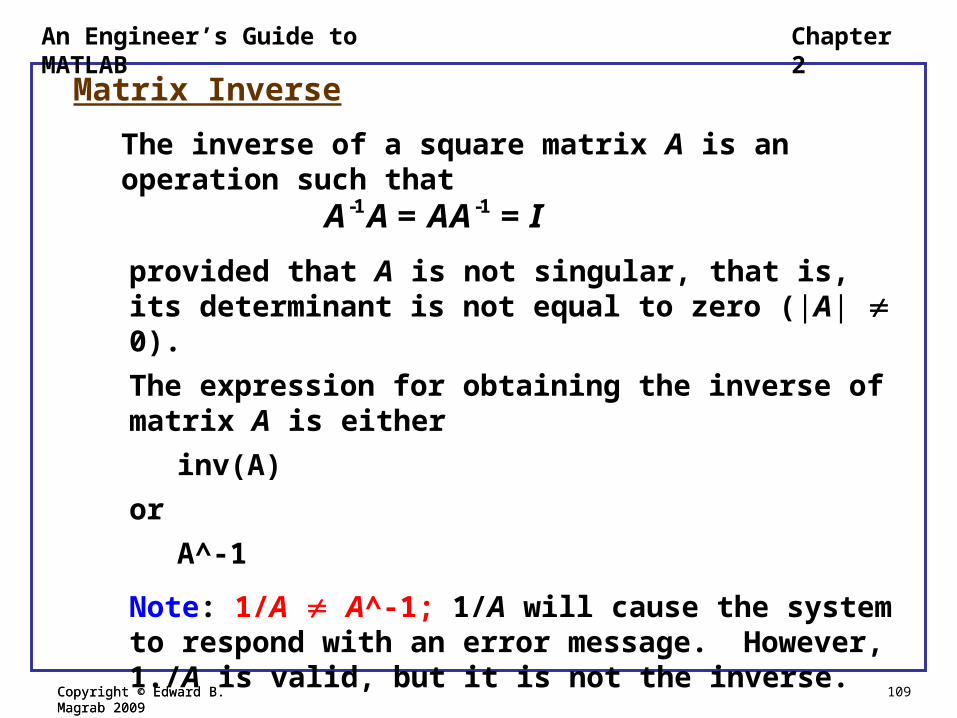
Matrix Inverse
The inverse of a square matrix A is an operation such that
-1 -1A A = AA = I
provided that A is not singular, that is, its determinant is not equal to zero (|A| 0).
The expression for obtaining the inverse of matrix A is either
inv(A)
or
A^-1
Note: 1/A A^-1; 1/A will cause the system to respond with an error message. However, 1./A is valid, but it is not the inverse.

Copyright © Edward B. Magrab 2009 110Copyright © Edward B. Magrab 2009
Chapter 2An Engineer’s Guide to MATLAB
Example - Inverse of Matrix
We shall determine the inverse of the magic matrix and the product of the inverse with the original matrix. The program is
invM = inv(magic(3))IdentMat = invM*magic(3)
Its execution gives
invM = 0.1472 -0.1444 0.0639 -0.0611 0.0222 0.1056 -0.0194 0.1889 -0.1028IdentMat = 1.0000 0 -0.0000 0 1.0000 0 0 0.0000 1.0000

Copyright © Edward B. Magrab 2009 111Copyright © Edward B. Magrab 2009
Chapter 2An Engineer’s Guide to MATLAB
Solution of a System of Equations
Consider the following system of n equations and n unknowns xk, k = 1, 2, …, n
11 1 12 2 1 1
21 1 22 2 2 2
1 1 2 2
+ + ... + =
+ + ... + =
...
+ + ... + =
n n
n n
n n nn n n
a x a x a x b
a x a x a x b
a x a x a x b
We rewrite this system of equations in matrix notation as follows:
Ax = b
where A is the following (nn) matrix

Copyright © Edward B. Magrab 2009 112Copyright © Edward B. Magrab 2009
Chapter 2An Engineer’s Guide to MATLAB
( )
11 12 1
21 22
1
...
...
... ...
...
n
n nn
a a a
a aA n n
a a
( ) ( )
1 1
2 21 and 1... ...
bn n
x b
x bx n b n
x
and
The symbolic solution is obtained by pre-multiplying both sides of the matrix equation by A-1. Thus,
since A-1A = I, the identity matrix, and Ix = x.
1 1
1
A Ax A b
x A b

Copyright © Edward B. Magrab 2009 113Copyright © Edward B. Magrab 2009
Chapter 2An Engineer’s Guide to MATLAB
The preferred expression for solving this system of equations is
x = A\b
where the backslash operator indicates matrix division and is referred to by MATLAB as left matrix divide. An equivalent way of solving a system of equations is by using
x = linsolve(A, b)

Copyright © Edward B. Magrab 2009 114Copyright © Edward B. Magrab 2009
Chapter 2An Engineer’s Guide to MATLAB
Example –
Consider the following system of equations
1 2 3
1 2 3
1 2 3
8 + + 6 = 7.5
3 + 5 + 7 = 4
4 + 9 + 2 = 12
x x x
x x x
x x x
which, in matrix notation, is
1
2
3
8 1 6 7.5
3 5 7 4
4 9 2 12
x
x
x
We shall determine xk and verify the results.

Copyright © Edward B. Magrab 2009 115Copyright © Edward B. Magrab 2009
Chapter 2An Engineer’s Guide to MATLAB
A = [8, 1, 6; 3, 5, 7; 4, 9, 2];b = [7.5, 4, 12]';x = A\b
z = A*x
which, upon execution, gives
x = 1.2931 0.8972 -0.6236
z = 7.5000 4.0000 12.0000
1
2
3
8 1 6 7.5
3 5 7 4
4 9 2 12
x
x
x

Copyright © Edward B. Magrab 2009 116Copyright © Edward B. Magrab 2009
Chapter 2An Engineer’s Guide to MATLAB
Example – Temperatures in a Slab
A thin square metal plate has a uniform temperature of 80 C on two opposite edges and a temperature of 120 C on the third edge and a temperature of 60 C on the remaining edge.
A mathematical procedure to approximate the temperature at six uniformly spaced interior points results in the following equations.
1 2 6
1 2 3 5
2 3 4
3 4 5
2 4 5 6
1 5 6
4 200
4 80
4 140
4 140
4 80
4 200
T T T
T T T T
T T T
T T T
T T T T
T T T

Copyright © Edward B. Magrab 2009 117Copyright © Edward B. Magrab 2009
Chapter 2An Engineer’s Guide to MATLAB
The temperatures are determined from the following script.
c = [4 -1 0 0 0 -1 -1 4 -1 0 -1 0 0 -1 4 -1 0 0 0 0 -1 4 -1 0 0 -1 0 -1 4 -1 -1 0 0 0 -1 4];d = [200, 80, 140, 140, 80, 200];T = linsolve(c, d')
The execution of this script gives T = 94.2857 82.8571 74.2857 74.2857 82.8571 94.2857
1 2 6
1 2 3 5
2 3 4
3 4 5
2 4 5 6
1 5 6
4 200
4 80
4 140
4 140
4 80
4 200
T T T
T T T T
T T T
T T T
T T T T
T T T