An Empirical Test of the Fama-French Five-Factor …...AN EMPIRICAL TEST OF THE FAMA-FRENCH...

AN EMPIRICAL TEST OF THE FAMA-FRENCH FIVE-FACTOR MODEL

Applicability to Equitized State-Owned Enterprises in Vietnam

Master’s Thesis

Nguyen Nhat Minh

Aalto University School of Business

Finance

Spring 2018

Aalto University, P.O. BOX 11000, 00076 AALTO

www.aalto.fi

Abstract of master’s thesis

Author Nguyen Nhat Minh

Title of thesis An Empirical Test of the Fama-French Five-Factor Model: Applicability to State-Owned

Enterprises in Vietnam

Degree Master of Science in Economics and Business Administration

Degree programme Finance

Thesis advisor(s) Sami Torstila

Year of approval 2018 Number of pages 84 Language English

Abstract

Research Objectives – Asset pricing is one of the most popular topics in financial economics that has been

studied for decades as various theories and models were established in this field. However, most of these

studies were conducted for the markets in the United States or other developed countries, which can have

questionable implications in the emerging and frontier markets. Thus, this thesis aims to fill the research gap

by selecting Vietnam’s stock market as the market of interest. Besides, this thesis also explores a special

segment pertaining to the market: equitized state-owned enterprises (SOEs) by investigating the relationship

between average stock returns and state-ownership status. With respect to the model of interest, this thesis

will focus on the Fama-French five-factor model and its relative performance to others including the Capital

Asset Pricing Model (CAPM) and the Fama-French three-factor model. The underlying rationale for this

selection is that the five-factor is a recent model, which was first introduced in 2015, and since then there have

been mixed results from empirical tests of this model across different markets. Therefore, there emerges a

need to conduct research on this topic, especially for a developing and under-researched market like Vietnam.

Data & Methodology – The thesis will examine monthly returns of common stocks listed on both Ho Chi

Minh Stock Exchange and Hanoi Stock Exchange from July 2009 to December 2017, 102 months in total.

The sample will be rebalanced annually in June from 2009 to 2017. The sample size amounts to 620 companies

after the last rebalance in June 2017. Asset pricing tests will be implemented to investigate the explanatory

performance of each model by regressing excess returns of test portfolios on factor returns. Besides, the factor

spanning tests will help to determine whether any factor in the five-factor model is redundant by regressing

each of the five factors on the other four. All regressions will be conducted using the ordinary least squares

(OLS) method.

Main Findings – Regarding asset pricing tests, all models fare worst in 12 value-weighted test portfolios

formed from size and state capital. Specifically, the lethal portfolio for all tested models except CAPM

contains large stocks of firms with low state capital (state owns more than 0% and less than 50% of charter

capital). The average adjusted R2s of the CAPM, the three-factor model, and the five-factor model are

respectively 45.6%, 69.8%, and 70.6%. Regarding the factor redundancy issue, High-Minus-Low (HML) is

not a redundant factor in this empirical test. Instead, Robust-Minus-Weak (RMW) and Conservative-Minus-

Aggressive (CMA) appear to be the potential candidates. In general, this thesis provides a cautious support

for the superiority of the five-factor model over the CAPM and the three-factor model after assessing a

combination of criteria. It is important to view the superiority of the five-factor model with caution since

differences in performance between it and the three-factor model are hardly noticeable in many cases.

Furthermore, despite its superior performance, the five-factor model cannot fully capture average returns in

Vietnam’s stock market as it fails when test portfolios are formed from state capital, which is not explicitly

targeted by design.

Keywords asset pricing model, Fama French, five-factor model, three-factor model, CAPM, Vietnam, state

ownership

Table of Contents

1 Introduction ................................................................................................................. 1

1.1 Research Motivation ............................................................................................ 1

1.2 Research Questions .............................................................................................. 1

1.3 Research Contribution ........................................................................................ 2

1.4 Background – Vietnam’s Stock Market.............................................................. 3

1.4.1 Overview and Development ............................................................................... 3

1.4.2 Limitations and Challenges ................................................................................ 5

1.4.3 Stock Exchanges ................................................................................................ 6

1.4.4 SOE Equitization Program ................................................................................. 6

1.5 Main Findings ...................................................................................................... 7

1.6 Structure of the Thesis ......................................................................................... 8

2 Literature Review ...................................................................................................... 10

2.1 Efficient Market Hypothesis.............................................................................. 10

2.1.1 Definition and Foundation ............................................................................... 10

2.1.2 Different Forms and Implications ..................................................................... 10

2.1.3 Joint Hypothesis Problem ................................................................................ 11

2.2 Modern Portfolio Theory .................................................................................. 11

2.3 Capital Asset Pricing Model .............................................................................. 12

2.3.1 Core Concepts ................................................................................................. 12

2.3.2 Theoretical Criticism ....................................................................................... 14

2.3.3 Empirical Evidence and Anomalies .................................................................. 14

2.3.4 CAPM Extensions ........................................................................................... 15

2.4 Fama – French Three-Factor Model ................................................................. 16

2.5 Fama – French Five-Factor Model ................................................................... 17

2.5.1 Foundation ....................................................................................................... 17

2.5.2 Model Specification ......................................................................................... 19

2.5.3 Empirical Evidence .......................................................................................... 20

2.6 Previous Studies on Fama – French Models in Vietnam’s Stock Market ....... 24

3 Hypotheses ................................................................................................................. 28

4 Data and Methodology .............................................................................................. 30

4.1 Sample Description ............................................................................................ 30

4.2 Variable Construction ....................................................................................... 31

4.2.1 Independent variables ...................................................................................... 31

4.2.2 Dependent variable .......................................................................................... 34

4.3 Asset Pricing Tests ............................................................................................. 34

4.4 Factor Spanning Tests ....................................................................................... 35

5 Findings and Discussion ............................................................................................ 37

5.1 The Playing Field ............................................................................................... 37

5.1.1 Size Effect ....................................................................................................... 37

5.1.2 Value Effect ..................................................................................................... 40

5.1.3 Profitability Effect ........................................................................................... 40

5.1.4 Investment Effect ............................................................................................. 40

5.1.5 State-ownership Effect ..................................................................................... 40

5.1.6 Other Patterns .................................................................................................. 41

5.2 Summary Statistics for Factor Returns ............................................................ 41

5.3 Correlations between Factors ............................................................................ 44

5.4 Asset Pricing Test Results ................................................................................. 45

5.4.1 Overview ......................................................................................................... 45

5.4.2 Size – B/M Portfolios ....................................................................................... 49

5.4.3 Size – OP Portfolios ......................................................................................... 54

5.4.4 Size – Inv Portfolios......................................................................................... 58

5.4.5 Size – SO Portfolios ......................................................................................... 62

5.5 Factor Spanning Test Results ............................................................................ 67

6 Conclusion ................................................................................................................. 70

6.1 Main Findings .................................................................................................... 70

6.2 Limitation and Suggestion for Further Research ............................................. 73

6.3 Concluding Remarks ......................................................................................... 74

7 References .................................................................................................................. 76

8 Appendices ................................................................................................................. 80

Appendix A .................................................................................................................... 80

Appendix B .................................................................................................................... 81

Appendix C .................................................................................................................... 83

1

1 INTRODUCTION

1.1 Research Motivation

Asset pricing is one of the most popular topics in financial economics that has been studied for

decades as various theories and models were established in this field. However, most of these

studies were conducted for the markets in the United States (US) or other developed countries,

which can have questionable implications in the emerging and frontier markets. Therefore, this

thesis aims to fill the research gap by selecting Vietnam’s stock market as the market of interest.

Vietnam’s stock market is currently a fledgling and small market with remarkable growth in

recent years. However, compared to other markets in developed countries, it still has several

limitations such as limited investing and trading products, limited transparency, or incidents

related to price manipulation. Given these drawbacks and lack of research attention, it would

be interesting to see whether there are any noticeable differences in the performance of asset

pricing models between Vietnam’s stock market and other markets.

Besides the Vietnam’s stock market as a whole, this thesis also explores a special segment

pertaining to the market: equitized state-owned enterprises (SOEs). In Vietnam, equitization of

an SOE is defined as the act of transforming that SOE into a joint stock company. By the term

“Equitized SOE”, this thesis refers to a joint stock company which is a former SOE but now

jointly owned by the state and the private sector. The equitization program has been a key bullet

point on Vietnamese government’s agenda since the 90s, with the goal to increase the

efficiency of these enterprises and restructure the economy. As equitized SOEs play a crucial

role in Vietnam’s stock market, this segment deserves research attention from my perspective.

With respect to the model of interest, this thesis will focus on the Fama-French (henceforth FF)

five-factor asset pricing model and its relative performance to others. The underlying rationale

for this selection is that FF five-factor is a recent model, which was first introduced in the

Journal of Financial Economics in 2015, and since then there have been mixed results from

empirical tests of this model across different markets. Thus, there emerges a need to conduct

research on this topic, especially for a developing and under-researched market like Vietnam.

1.2 Research Questions

In general, this thesis aims to answer three main research questions, stated as follows:

1. To what extent can Vietnam’s average stock returns be explained by the five-factor

model?

2

2. To what extent can average stock returns of Vietnamese equitized SOEs be explained

by the five-factor model?

3. Is there any factor in the five-factor model whose effect is fully absorbed by other

factors in the case of Vietnam’s stock market?

1.3 Research Contribution

Originally developed from a sample of US stocks during 1963-2013, the Fama-French five-

factor model is an empirically motivated asset pricing model, which raises concerns about data

mining and thus necessitates out-of-sample tests. Therefore, the first and foremost contribution

of this thesis is to provide an out-of-sample test for the model in Vietnam’s stock market,

adding to the comparative evidence across international markets.

Furthermore, this thesis also contributes to the existing literature regarding FF empirical tests

in Vietnam’s stock market in many ways. Firstly, this thesis extends the test period with much

more recent data – nearly nine years from July 2009 to December 2017. Most of FF empirical

tests in Vietnam’s stock market are dated and cover only a short period, which results in small

sample size and observation scarcity given the primitive stage of the market at that time.

Secondly, this thesis also expands the test by including the recent FF five-factor model, which

was firstly introduced by Fama and French in 2015. As abovementioned, the majority of FF

empirical tests in Vietnam’s stock market are dated and thus they only apply the FF three-factor

model. Thirdly, this thesis implements a formal test, the GRS test1, to examine models’

explanatory capability. Most previous studies do not use any formal test for performance

assessment but only compare average adjusted R2s among models and count how many

regression intercepts are statistically significant. Finally, this thesis explores the relationship

between expected stock returns and state ownership by investigating the capability of FF

models in explaining average stock returns of equitized SOEs. Forming test portfolios from

state capital rather than the same variables used to construct risk factors also serves as a robust

test for the models.

Besides contributing to the existing literature, the thesis also has practical implications for

management. It will to help determine which model among the CAPM, the three-factor model,

1 GRS test, derived by Gibbons, Ross, and Shanken (1989), is used to test the null hypothesis that intercepts from

asset pricing regressions are jointly equal zero, implying that the asset pricing model can fully explain average

returns. An asset pricing model will pass the test if this null hypothesis cannot be rejected and vice versa. Lower

GRS statistic is often interpreted as better model performance.

3

and the five-factor model is an appropriate tool for practical applications such as portfolio

performance evaluation and cost-of-equity estimation in Vietnam’s stock market. For the

moment, CAPM is undoubtedly the most frequently used model in these applications thanks to

its elegance and parsimony, also for which it has received various criticisms both theoretically

and empirically2. Therefore, the need for other models emerges.

1.4 Background – Vietnam’s Stock Market

As Vietnam’s stock market is the focus of this thesis, this section will briefly discuss the

development, potential and limitation of the market as well as Vietnam’s equitization program.

This section aims to provide background knowledge and set the context for the study.

1.4.1 Overview and Development

Given its young age and small size, Vietnam’s stock market is considered a developing market.

To avoid confusion for some readers, the term “emerging market” will not be used when

referring to Vietnam since it is a matter of classification that “emerging market” will be

assessed differently across agencies. For example, Vietnam is considered a frontier (pre-

emerging) market by Morgan Stanley Capital International (MSCI) but is included in the

Emerging Markets Bond Index by J.P. Morgan.

Vietnam’s stock market was officially established in July 1998, but not until July 28, 2000 did

the first trading day take place with only two listed stocks. Besides its young age, Vietnam’s

stock market is relatively small compared to other markets in Southeast Asia. For example,

market capitalization of listed domestic companies as a percentage of GDP of Vietnam in 2016

is only 32.8% while those of Singapore, Malaysia, and Thailand are respectively 215.7%,

121.4%, and 106.4% (The World Bank). Figure 1 shows this ratio year-over-year from 1998

to 2016 of six Southeast Asian countries. From this visual representation, it is easy to notice

that Vietnam lies on the lowest line in the chart.

2 To be discussed in Section 2.3.2 and 2.3.3

4

Figure 1 Market Capitalization of listed domestic companies as % of GDP (Adapted from: The World

Bank - Data)

Despite its small scale, Vietnam’s stock market is undoubtedly one of the fastest growing

markets in the world with great potential and enormous room for improvement. According to

updated information from Vietnam Ministry of Finance, Vietnam’s total market capitalization

reached 74.6% of GDP at the end of 2017 (VietStock, 2017). This statement can be further

verified by the evolution of the Vietnam Stock Index (VN-Index), a capitalization-weighted

index of all listed companies on Ho Chi Minh City Stock Exchange with a base index value of

100 as of July 28, 2000.

Figure 2 VN-Index from July 28, 2000 to December 29, 2017 (Adapted from: VNDirect)

Figure 2 shows the development of VN-Index from its inception to December 29, 2017. In the

period 2000 – 2005, the market remained dormant most of the time with low trading volume.

5

However, starting from 2006, prices started to pick up and there was also an increase in trading

volume. This uptrend was consistent until March 13, 2007 when VN-Index reached its all-time

high of 1178.67 points, nearly triple in only one year. After reaching its peak, VN-Index

fluctuated wildly till the end of 2007 and started to plunge throughout 2008 and the first quarter

of 2009. The period from 2006 to 2008 is considered the boom-and-burst period in Vietnam’s

stock market that took place due to a combination of factors, including but not limited to

irrationally high expectation, unstainable growth, herd mentality, and lax credit policy.

From the second quarter of 2009, Vietnam’s stock market began to recover and regain investor

confidence, which resulted in an increase in trading volume. However, not until 2013 did the

stock market fully recuperate from the recession. Since then, VN-Index has become more

stable and grown consistently over years. From Dec 28, 2012 to December 29, 2017, VN-Index

grew at a CAGR of approximately 18.7%/year. In 2017, the index recorded its highest annual

growth in the last 10 years of approximately 51.5%, ending the year at 10-year high.

1.4.2 Limitations and Challenges

Although having a promising future, Vietnam’s stock market currently encounters numerous

limitations and challenges, of which this thesis will name a few. Firstly, trading volume is low

in some stocks due to small market size. Together with inadequate supervision, low liquidity

has created loopholes for price manipulation. For example, in September 2017, a man was

fined 550 million VND by the State Securities Commission for using 28 different trading

accounts to create fake supply and demand for stock ticker VMD for five months (Bao Moi,

2017). Another major case is about a woman who was fined 600 million VND for using 42

different accounts to manipulate the price of stock ticker HNG (ibid.). While these two cases

are the most recent, there are other major and minor cases in the past, which are not hard to

find on the internet with the keyword “stock price manipulation” written in Vietnamese.

Another challenge that Vietnam’s stock market confronts is transparency, which must be

guaranteed to protect the benefits of current investors as well as to build trust and attract

prospective ones. Since the inception, there has been a significant progress in ensuring

information transparency in Vietnam’s stock market. For example, the State Securities

Commission has attempted to revise the legal framework, require listed companies to disclose

information in English, and consider the application of IFRS for listed companies (VN

Securities Investment, 2017). Nevertheless, there is still a huge gap compared to the

international standards. Incidents related to falsified information, fake news, price

6

manipulation, mismatch in information disclosure, or delay in disclosing financial reports still

persist and happen sometimes. However, it is interesting to see how the asset pricing models

perform given the presence of these factors.

1.4.3 Stock Exchanges

Vietnam has two main stock exchanges: Ho Chi Minh City Stock Exchange (HOSE or HSX)

and Hanoi Stock Exchange (HNX). In addition to these two main exchanges, there is another

one organized by HNX called UPCoM, short for Unlisted Public Company Market. UPCoM,

founded in 2009, is an exchange where public companies that are not listed on either HOSE or

HNX are traded. However, this thesis will not take UPCoM into account since it only concerns

listed stocks. Table 1 presents some key information about these two main exchanges.

Table 1 Basic information about Ho Chi Minh City Stock Exchange (HOSE) and Hanoi Stock Exchange

(HNX) as at 31/12/2017 (Adapted from: hnx.vn, hsx.vn)

HOSE HNX

Year of establishment 2000 2005

Main index VN-Index HNX-Index

Market cap (VND billion) 2,101,209 92,796

Number of listed stocks 340 378

1.4.4 SOE Equitization Program

In the context of Vietnam’s stock market, equitization can be understood as the transformation

of SOEs into joint stock companies by sale of shares through public auction or by private

agreement with strategic investors (Allens Linklaters, 2017). As aforementioned, equitization

of SOEs has been a key bullet point on the Vietnamese government’s agenda. For the past 15

years, the number of SOEs has dropped sharply from about 6,000 to over 700 (Vietnam News,

2016). From 2011 to 2015, nearly 600 SOEs were equitized, which completed 96% of the target

number (ibid.).

7

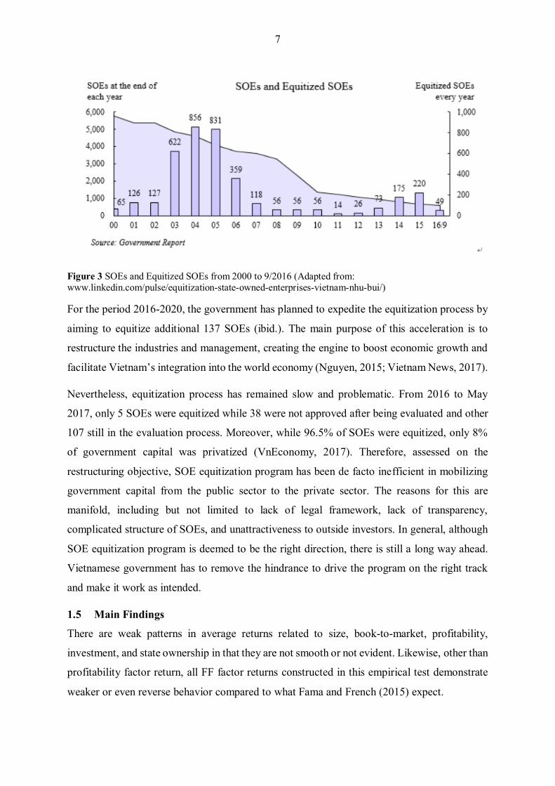
Figure 3 SOEs and Equitized SOEs from 2000 to 9/2016 (Adapted from:

www.linkedin.com/pulse/equitization-state-owned-enterprises-vietnam-nhu-bui/)

For the period 2016-2020, the government has planned to expedite the equitization process by

aiming to equitize additional 137 SOEs (ibid.). The main purpose of this acceleration is to

restructure the industries and management, creating the engine to boost economic growth and

facilitate Vietnam’s integration into the world economy (Nguyen, 2015; Vietnam News, 2017).

Nevertheless, equitization process has remained slow and problematic. From 2016 to May

2017, only 5 SOEs were equitized while 38 were not approved after being evaluated and other

107 still in the evaluation process. Moreover, while 96.5% of SOEs were equitized, only 8%

of government capital was privatized (VnEconomy, 2017). Therefore, assessed on the

restructuring objective, SOE equitization program has been de facto inefficient in mobilizing

government capital from the public sector to the private sector. The reasons for this are

manifold, including but not limited to lack of legal framework, lack of transparency,

complicated structure of SOEs, and unattractiveness to outside investors. In general, although

SOE equitization program is deemed to be the right direction, there is still a long way ahead.

Vietnamese government has to remove the hindrance to drive the program on the right track

and make it work as intended.

1.5 Main Findings

There are weak patterns in average returns related to size, book-to-market, profitability,

investment, and state ownership in that they are not smooth or not evident. Likewise, other than

profitability factor return, all FF factor returns constructed in this empirical test demonstrate

weaker or even reverse behavior compared to what Fama and French (2015) expect.

8

Regarding asset pricing tests, all models fare worst in 12 value-weighted test portfolios formed

from size and state capital when assessed by either GRS statistics or average absolute values

of intercepts. Specifically, the lethal portfolio for all tested models except CAPM contains large

stocks of firms with low state capital (state owns more than 0% and less than 50% of charter

capital). The average adjusted R2s of the CAPM, the three-factor model, and the five-factor

model are respectively 45.6%, 69.8%, and 70.6%.

Regarding the factor redundancy issue, High-Minus-Low (HML) is not a redundant factor in

this empirical test, which is different from the conclusion of Fama and French (2015). Instead,

Robust-Minus-Weak (RMW) and Conservative-Minus-Aggressive (CMA) become the

potential candidates. Both RMW and CMA slopes in the five-factor regressions are mainly not

statistically significant as their average returns are either largely or fully captured by exposure

to other factors, especially HML. Furthermore, the five-factor model shows paltry

improvement or even deterioration (assessed by average adjusted R2) from the five-factor

model that drops RMW or CMA. In the case of RMW, a possible explanation lies in the highly

negative correlation between it and HML over the sample period.

In general, this empirical test provides a cautious support for the superiority of the five-factor

model over the CAPM and the three-factor model after assessing their average adjusted R2s,

GRS statistics, and average absolute values of intercepts. Particularly, the five-factor model

produces the highest average adjusted R2, lowest GRS statistics in two out of four portfolio

sets, and lowest average absolute values of intercepts except in one set. It is important to view

the superiority of the five-factor model with caution since differences in performance between

it and the three-factor model are hardly noticeable in many cases. Furthermore, despite its

superior performance, the five-factor model cannot fully capture average returns in Vietnam’s

stock market. The model fails when test portfolios are formed from state capital, which is not

explicitly targeted by design.

1.6 Structure of the Thesis

The remainder of the thesis is structured as follows. Section 2 presents a review of the main

literature relevant to the topic, including Efficient Market Hypothesis, Modern Portfolio

Theory, Capital Asset Pricing Model, Fama-French Three-Factor Model, and Fama-French

Five-Factor Model. Afterwards, Section 3 outlines the key hypotheses of this thesis. Section 4

continues with details about sample description, variable construction, as well as specifications

of asset pricing and factor spanning tests. Subsequently, Section 5 provides a synthesis of

9

empirical test results together with an in-depth discussion about their possible causes and

implications. Finally, Section 6 concludes the thesis with summary of the main findings,

limitations of the study, suggestions for further research, and concluding remarks.

10

2 LITERATURE REVIEW

2.1 Efficient Market Hypothesis

2.1.1 Definition and Foundation

The efficient market hypothesis (EMH) is considered not only a cornerstone but also one of

the most debatable topics in the field of investment. An efficient market is defined as a market

where prices always “fully reflect” available information (Fama, 1970). With this definition,

the hypothesis asserts that investors cannot consistently beat the market.

According to Miller et al. (2011), the foundation of an efficient market lies at three main

conditions: investor rationality, independent deviations from rationality, and arbitrage. It is

important to note that rationality in this discussion only means investors do not systematically

overvalue or undervalue the assets given the information they have (ibid). If the first condition

is fulfilled that every investor is rational, he or she will have the same expected return for assets

at the same risk level, which eventually reflects in “correct” asset prices. Hence, consistently

earning excess return is extremely difficult if not improbable in this case. The second condition

maintains that even if investors are irrational, the market can still be efficient when their

irrationalities are not dependent and not heading in the same direction. For example, some

investors may overvalue while some may undervalue a certain financial asset. Together, their

contradictory valuations will offset one another and therefore irrationality will be diversified

away (ibid.). Nevertheless, irrationality is not always balanced. If this is the case, the market

can still be efficient if there is a group of rational investors who arbitrage away the mispricing

and make the market efficient again.

2.1.2 Different Forms and Implications

Fama (1970) classifies efficient market into three forms ranked on the information set they

entail, namely weak form, semi-strong form, and strong form, with the weaker nested in the

stronger (see Appendix A1 for a graphical presentation of different forms of EMH).

In weak-form efficient market, the current prices fully reflect all historical information such as

past prices and trading volume (ibid.), and thus the future stock prices will be independent of

these historical data. In other words, weak-form of EMH implies that future price movement

is unpredictable and exhibits a random walk. This implication means that technical analysis,

the practice of analyzing historical trading activity to forecast future price moment, will be

useless in this case.

11

In semi-strong-form efficient market, all publicly available information including historical

data is fully reflected in the current stock prices. Put differently, the stock prices will adjust

unbiasedly in a timely manner when there is new public information such as earning forecasts,

annual reports, or any relevant announcement. Therefore, in this form, neither technical nor

fundamental analysis will prove useful in beating the market.

In strong-form efficient market, all kind of information regardless private or public is fully

reflected in the current stock prices. That is, stock prices are unpredictable in every way and

even possessing insider information does not help to generate abnormal return.

2.1.3 Joint Hypothesis Problem

Although the hypothesis seems to be simple, it has been the center of disputes among

academics for decades and several studies were conducted to test its validity. The results from

these tests, however, are not straightforward conclusions of whether the market is efficient or

not due to the joint hypothesis problem. Since an asset pricing model is needed to validate

EMH, concluding that the market is inefficient can also mean the asset pricing model is mis-

specified. In other words, validating EMH by using an asset pricing model becomes a joint test

of both the EMH and the underlying model. Before the review of asset pricing models, it is

crucial to discuss the Modern Portfolio Theory, which set the foundation for many subsequent

papers on this topic.

2.2 Modern Portfolio Theory

In 1952, Markowitz introduced the Modern Portfolio Theory (MPT) for the first time in his

essay “Portfolio Selection”. The theory assumes that investors are risk-averse. That is,

investors will prefer a less risky portfolio to a riskier one given the same level of return or, in

other words, they will prefer a portfolio with higher return given the same level of risk. Under

this assumption, the theory implies that risk and return should be considered in tandem in that

higher risk should correspond to higher expected return and vice versa.

By consolidating these concepts, Markowitz (ibid.) presented a framework for constructing a

portfolio in which expected return is maximized for a certain level of risk. In this model, the

portfolio return is defined as the mean return, which is the weighted average return of all

component assets. On the other hand, the portfolio risk is defined as the portfolio variance3,

which is not the weighted average of individual assets’ variances. Instead, the portfolio

3 Portfolio risk can be also defined as the portfolio standard deviation (the square-root of variance).

12

variance is calculated by taking into account the standard deviations of component assets and

the correlation coefficients for each pair of assets. For example, considering a portfolio with

only two assets X and Y, its expected return 𝐸(𝑅𝑝) and variance 𝜎𝑝2 are calculated as follows:

𝐸(𝑅𝑝) = 𝑤𝑋𝐸(𝑅𝑋) + 𝑤𝑦𝐸(𝑅𝑦) (1)

𝜎𝑝2 = 𝑤𝑋

2𝜎𝑋2 + 𝑤𝑌

2𝜎𝑌2 + 2𝑤𝑋𝑤𝑌𝜎𝑋𝜎𝑌𝜌𝑥𝑦 ( |𝜌| ≤ 1) (2)

From Equation (2), we can notice that the portfolio variance can be reduced if the correlation

coefficient 𝜌𝑥𝑦 is much smaller than 1. A correlation coefficient of 1 means that the returns of

X and Y are always heading in the same direction by the same amount. On the other hand, a

correlation coefficient different than 1 means that the returns of X and Y vary in different

patterns, which may offset each other and effectively reduce the combination variance. This is

one of the most crucial points that Markowitz (ibid.) wants to deliver through his work. In

general, Markowitz (ibid.) states that investors can lower the portfolio risk by holding a

diversified combination of assets that are not perfectly and positively correlated. Thus,

diversification allows a portfolio with the same level of expected return to have lower risk.

Graphically, all possible combinations of risky assets that offer the highest expected return for

a certain level of risk (optimal portfolios) constitute a curve called the Efficient Frontier (see

Appendix A2). Any combinations that do not lie on the curve are considered sub-optimal since

they have a lower expected return given the same risk level compared to the optimal portfolios.

Note that risk-less asset is not on Markowitz’s Efficient Frontier.

Since its introduction, the MPT became the theoretical foundation for several research papers

at that time, which includes the Capital Asset Pricing Model.

2.3 Capital Asset Pricing Model

2.3.1 Core Concepts

The Capital Asset Pricing Model (CAPM) was independently developed by Sharpe (1964) and

Lintner (1965), built upon the Modern Portfolio Theory of Markowitz (1952, 1959). Before

discussing the model, it is necessary to review its underlying assumptions. Along with the

inherent assumptions in Markowitz’s model, the CAPM adds two more specialized and major

assumptions. Firstly, all investors are able to borrow and lend unlimitedly at the risk-free rate

of interest (Sharpe, 1964). Secondly, all investors have homogenous expectation; that is, they

unanimously agree on the characteristics of different investments such as expected values,

standard deviations, and correlation coefficients (ibid.).

13

The CAPM specifies that in equilibrium, there exists a linear relationship between the expected

return of an individual asset or a portfolio and the market risk (ibid.). In general, this linear

relationship can be expressed in the following formula:

𝐸(𝑅𝑖 ) = 𝑅𝑓 + 𝛽(𝐸(𝑅𝑚) − 𝑅𝑓) (3)

Where 𝑅𝑓 the risk-free rate of return, 𝐸(𝑅𝑚) the expected market return, and 𝛽 equals:

𝛽 =𝐶𝑜𝑣(𝑅𝑖 , 𝑅𝑚)

𝜎𝑚2

(4)

As aforementioned, the MPT shows that by holding a combination of different assets that are

not perfectly positively correlated, investors can cancel out the individual risks and help to

lower the overall risk of the portfolio. Nevertheless, Sharpe (ibid.) contends that this notion is

only a part of the whole picture since not all the risk can be diversified away. This type non-

diversifiable risk, termed systematic risk, represents the risk resulting from fluctuation in the

economy and remains even in efficient portfolios. Intuitively, since an asset itself is included

in the market, the asset’s rate of return unavoidably expresses some correlation to the market

fluctuation that cannot be diversified. The sources of systematic risk, for example, can be

changes in interest rate, market collapse, economic recession, or war, which inevitably affect

the whole economy and its markets.

Systematic risk is measured by the beta coefficient in the CAPM equation, which indicates the

responsiveness of an asset’s rate of return to changes in the economy. Since unsystematic risk

can be diversified away, the CAPM maintains that only the beta coefficient is appropriate in

assessing the risk of an asset (ibid.). In theory, an asset having a lower beta will have a lower

expected return as it tends to be safer (less responsive to market fluctuation) than assets with

higher beta.

Compared to Markowitz’s MPT, Sharpe-Lintner CAPM introduces a few extensions. Firstly,

CAPM can be used to determine the price of an individual asset. Secondly, the CAPM

considers the inclusion of risk-less assets in the market portfolio. In this case, the efficient

portfolios will lie on a straight line - Capital Market Line (CML), which is the tangent line of

Markowitz’s Efficient Frontier (see Appendix A3). Thirdly, the CAPM classifies risk into two

categories: systematic and unsystematic. The former type of risk is related to market fluctuation

and cannot be diversified away.

14

2.3.2 Theoretical Criticism

CAPM has undoubtedly become one of the most popular asset pricing models, which is taught

in every introductory finance class and used in several real-life applications such as assessing

portfolio performance, estimating cost of equity, or calculating abnormal returns. Nevertheless,

like any other models, the CAPM has inevitably received various criticisms both theoretically

and empirically.

From a theoretical perspective, the CAPM was criticized for its highly restrictive assumptions.

For example, the assumption that investors can borrow and lend unlimitedly at the risk-free

rate of return are apparently unrealistic. Likewise, unlimited short sales do not exist in real life

because of regulatory framework that restricts short-selling activities. Nevertheless, some of

these restrictive assumptions were relaxed in extension models (Celik, 2012). Regarding this

issue, even Sharpe (1964) himself admits that his model has “highly restrictive and

undoubtedly unrealistic assumptions” (p. 434). However, he also argues that a theory should

be appropriately tested by the eligibility of its implications rather than the realism of its

assumptions (ibid.).

2.3.3 Empirical Evidence and Anomalies

Besides theoretical criticisms, the CAPM also had questionable empirical applicability. In their

article “The Capital Asset Pricing Model: Theory and Evidence”, Fama and French (2004)

frankly state that Sharpe-Lintner CAPM “has never been an empirical success” (p. 43). This

literature review will discuss a few prominent empirical tests of CAPM.

Among the early tests was a study conducted by Basu (1977), who investigates the relationship

between Price-to-Earning (P/E) ratio and US stock returns. The author (ibid.) find that low P/E

securities on average tend to have higher risk-adjusted returns than high P/E securities during

April 1957 – March 1971. This phenomenon can generally be classified as value effect, which

CAPM failed to explain.

Rosenberg, Reid, and Lanstein (1985) provide further evidence for value effect in US stock

returns. Their research results show that during the period 1980-1984, firms with high Book-

to-Market equity (B/M), on average, yield higher risk-adjusted returns than firms with low

B/M. Similar to Rosenberg et al., Stattman (1980) also documents a positive relationship

between average stock returns and B/M ratio in US’ stock market. Furthermore, this

relationship is also discovered in Japan’s stock market by Chan, Hamao, and Lakonishok

(1992).

15

Improving upon Basu’s study (1977), Reiganum (1981) examines the relationship of Earning-

to-Price (E/P) ratio, firm size, and US stock returns in the period 1962-1978. Like Basu’s

results, Reiganum’s show that portfolios with high E/P seem to outperform ones with low E/P

even after adjusting for CAPM’s beta risk. Moreover, Reiganum (1981) also finds that small

firms, on average, generate significantly higher returns than large firms after adjusting for beta

risk for at least two years. However, the E/P effect will disappear when taking the size effect

into consideration while the size effect persists after controlling for the E/P effect (ibid.). In

brief, Reiganum (ibid.) concludes that the CAPM is mis-specified and the source of

misspecification comes from the missing risk factors that are closely related to size effect.

Banz (1981) also investigates the relationship between size effect and US stock returns but for

a much longer period (1926 - 1975) compared to Reiganum’s study. Like Reiganum, the author

also documents a size effect in US stock returns although this effect is unstable across sub-

periods. Banz (ibid.) finds that small NYSE firms, on average, have significantly higher risk-

adjusted returns than large NYSE firms over a 40-year period.

In general, all the phenomena discussed above are called anomalies, which are “empirical

results that seem to be inconsistent with maintained theories of asset pricing behavior”

(Schwert, 2003). Besides anomalies related to size and value, there are also other types such as

momentum, reversal effect, January effect, or day-of-the-week effect. These anomalies tend to

behave differently in that they might persist, attenuate, reverse or disappear over time. Due to

the joint hypothesis problem, the reason for anomaly’s existence can be either that the market

is not efficient or that the asset pricing model is mis-specified. However, academics usually

attribute anomalies to CAPM misspecification rather than market inefficiency (Basu, 1977;

Ball, 1978; Reiganum, 1981; Banz, 1981; Fama and French, 1992). Regarding this issue, it is

intuitive and reasonable to argue that CAPM beta is not the sole factor to explain variation in

stock returns.

2.3.4 CAPM Extensions

Although having limitations, Sharpe-Lintner CAPM was undeniably the groundwork for the

development of other asset pricing models, which mostly are CAPM extensions by adapting

the original theoretical framework to enhance empirical applicability. These extensions are the

results from various empirical tests, which discovered additional variables that help explain

average stock returns in addition to CAPM beta. Figure 4 below shows the development and

extension of CAPM until 2012.

16

Figure 4 Theoretical development of CAPM till 2012 (Adapted from: Celik, 2012)

2.4 Fama – French Three-Factor Model

Inspired by previous CAPM empirical tests, Fama and French (1992) attempt to evaluate how

market beta, size, E/P, leverage, and B/M can jointly explain the cross-section of average stock

returns. The findings show that size and B/M are the two variables that capture much of the

variation in US average stock returns associated with size, E/P, leverage, and B/M for the 1963-

1990 period (ibid.).

In the subsequent paper “Common risk factors in the returns on stocks and bonds”, Fama and

French (1993) conclude that size (measured by market equity) and value (measured by B/M)

are the proxies for sensitivity to common risk factors in stock returns. The authors then

incorporate these two variables in their asset pricing model, namely the Fama-French three-

factor model. In general, this model can be expressed in the following time-series regression:

𝑅𝑖𝑡 − 𝑅𝐹𝑡 = 𝑎𝑖 + 𝑏𝑖(𝑅𝑀𝑡 − 𝑅𝐹𝑡) + 𝑠𝑖𝑆𝑀𝐵𝑡 + ℎ𝑖𝐻𝑀𝐿𝑡 + 𝑒𝑖𝑡 (5)

where

𝑅𝑖𝑡: return on security or portfolio 𝑖 for period 𝑡

𝑅𝑀𝑡: return on value-weighted market portfolio

17

𝑅𝐹𝑡: risk-free return

𝑅𝑀𝑡 − 𝑅𝐹𝑡: market excess return (market premium)

𝑆𝑀𝐵𝑡: size premium (small minus big)

𝐻𝑀𝐿𝑡: value premium (high minus low)

𝑎𝑖: regression intercept

𝑏𝑖: measure of sensitivity to market fluctuation

𝑠𝑖: measure of sensitivity to size premium

ℎ𝑖: measure of sensitivity to value premium

𝑒𝑖𝑡: a zero-mean residual

The two additional variables besides market excess return are SMB – the difference between

returns on diversified portfolios of small and big companies, and HML– the difference between

returns on diversified portfolios of high B/M and low B/M companies. Since SMB and HML

aim to mimic the risk factors in returns related to size and value respectively, they are also

known as mimicking portfolios.

By regressing the excess returns of 25 test portfolios sorted by size and B/M4 on market excess

return, SMB, and HML, Fama and French find that the three-factor model outperforms CAPM

since most of the intercepts from three-factor regression are close to 0 (ibid.). The authors

further test the robustness of the three-factor model by regressing five portfolios formed on

earning yield (E/P) and other five formed on dividend yield (D/P). The results from these

regressions are equivalent to those from size – B/M portfolio regressions as the intercepts are

mostly close to 0 both statistically and practically (ibid.).

2.5 Fama – French Five-Factor Model

2.5.1 Foundation

In the 2006 paper “Profitability, investment and average returns”, Fama and French conduct

an empirical test of the Miller Modigliani valuation formula (1961), which holds that expected

stock returns are related to B/M, expected profitability, and expected investment. This formula

4 Constructed by 5 x 5 sort based on quintiles of size and B/M.

18

lays the foundation for the inclusion of two new factors in the Fama – French five-factor model

(2015) and it is therefore worth discussing.

To begin with, the market value of a firm’s equity, as in the dividend discount model, equals

the present value of expected dividends:

𝑀𝑡 = ∑ 𝐸(𝐷𝑡+𝜏)/(1 + 𝑟)𝜏 (6)

∞

𝑡=1

where 𝑀𝑡 is the market value of equity at time 𝑡, 𝐸(𝐷𝑡+𝜏) the expected dividend in the period

𝑡 + 𝜏, and 𝑟 the long-term average expected stock return. With clean surplus accounting, the

dividend discount formula can be equivalently transformed into:

𝑀𝑡 = ∑ 𝐸(𝑌𝑡+𝜏 − 𝑑𝐵𝑡+𝜏)/(1 + 𝑟)𝜏 (7)

∞

𝑡=1

where 𝑌𝑡+𝜏 is the total equity earnings for period 𝑡 + 𝜏, and 𝑑𝐵𝑡+𝜏 = 𝐵𝑡+𝜏 − 𝐵𝑡+𝜏−1 is the

change in total book equity in the period 𝑡 + 𝜏. Finally, dividing Equation (7) by book equity

at time 𝑡 results in:

𝑀𝑡

𝐵𝑡=

∑ 𝐸(𝑌𝑡+𝜏 − 𝑑𝐵𝑡+𝜏)/(1 + 𝑟)𝜏 ∞𝑡=1

𝐵𝑡 (8)

Equation (8) can be referred as the Miller Modigliani (1961) valuation formula. In this

equation, the expected total equity earning to current book equity is a measure of profitability

while the expected change in total book equity to current book equity is a measure of

investment. Therefore, Equation (8) generally comprises four terms: current B/M, expected

profitability, expected investment, and expected stock return. Controlling for two of these four

terms will demonstrate a direct relationship, either positive or negative, between the other two.

Specifically, holding all else constant, there exists a positive relationship between current B/M

and expected stock return, a positive relationship between expected profitability and expected

stock return, and a negative relationship between expected investment and expected stock

return.

Fama and French (2006) attempt to test these theoretical relationships empirically. The authors

argue that although their results tend to be in line with the predicted relationships and the

existing evidence from others, profitability and investment factors add little or nothing to the

explanation of stock return provided by size and B/M. Nevertheless, this conclusion has

19

received disagreement from other researchers, notably Novy-Marx (2013) and Aharoni,

Grundy, and Zeng (2013).

As abovementioned, Fama and French (2006) state that profitability factor does not play an

important role in enhancing the explanation of stock return provided by size and value factors.

However, Novy-Marx (2013) succeed in identifying a proxy for expected profitability that is

strongly related to average stock return. Concerning Fama and French’s study (2006), Novy-

Marx (2013) argue that the main difference is in the choice of proxy for future profitability.

While Fama and French (2006) select current earning, Novy-Marx (2013) chooses gross profit

as the proxy for future profitability. He maintains that gross profit is the “cleanest accounting

measure of true economic profitability”, which is unaffected by expensed investments such as

R&D or advertisement (ibid.).

Fama and French (2006) also receive criticism in terms of methodology from Aharoni et al.

(2013). In their 2006 paper, Fama and French fail to find the predicted negative relationship

between expected investment and stock return as they document a positive insignificant

coefficient for expected investment at the per-share level. However, Aharoni et al. (2013) argue

that the valuation formula does not necessarily hold at the per-share level and thus per-share

numbers can be misleading since they are influenced by changes in the number of shares (issues

or repurchases). When empirically investigating the valuation formula at the firm level,

Aharoni et al. (ibid.) indeed find a statistically significant negative relationship between

expected investment and average stock return as predicted.

2.5.2 Model Specification

Motivated by the valuation formula and the mounting evidence that the three factors cannot

explain much of the stock return variation related to profitability and investment, Fama and

French (2015) decide to add profitability and investment factors to the three-factor model. In

general, the Fama – French five-factor model is specified as follows:

𝑅𝑖𝑡 − 𝑅𝐹𝑡 = 𝑎𝑖 + 𝑏𝑖(𝑅𝑀𝑡 − 𝑅𝐹𝑡) + 𝑠𝑖𝑆𝑀𝐵𝑡 + ℎ𝑖𝐻𝑀𝐿𝑡 + 𝑟𝑖𝑅𝑀𝑊𝑡 + 𝑐𝑖𝐶𝑀𝐴𝑡 + 𝑒𝑖𝑡 (9)

where

… (similar to Equation 5)

𝑅𝑀𝑊𝑡: profitability premium (robust minus weak)

𝐶𝑀𝐴𝑡: investment premium (conservative minus aggressive)

20

𝑟𝑖: measure of sensitivity to profitability premium

𝑐𝑖: measure of sensitivity to investment premium

Among the two additional variables is RMW – the difference between returns on diversified

portfolios of firms with robust and weak profitability, measured by operating profit (OP).

However, OP in the five-factor model context is defined as revenues minus cost of goods sold

(COGS), selling, general, and administrative expenses (SG&A), and interest expenses, all

divided by book equity. The other additional variable is CMA – the difference between returns

on diversified portfolios of firms with conservative and aggressive investment, measured by

lagged total asset growth.

Regarding the sample of US stocks from July 1963 to December 2013, the five-factor model

indeed outperforms both the CAPM and the three-factor model, explaining 71%-94% of the

variation in stock returns. Furthermore, the five-factor model is also insensitive to the way its

factors are constructed. That is, although various ways of sorting are applied to construct the

explanatory variables, they all yield similar description of the average stock returns on the test

portfolios. Nevertheless, the model inevitably has a few limitations. Concerning the sample of

US stocks that Fama and French (2015) investigate, the five-factor model fails to explain low

average returns on small stocks whose returns behave like those of companies that invest

heavily despite low profitability. Moreover, HML factor appears to be redundant for describing

average stock returns when RMW and CMA factors are included. As one of the research

objectives, this thesis is interested in testing whether these limitations still hold and whether

new limitations can be discovered in the sample of Vietnamese stocks.

2.5.3 Empirical Evidence

Empirical test results for the Fama-French five-factor model are mixed, varying across

different markets and test periods. This literature review will mention a few prominent tests of

the five-factor model in markets around the world.

The first empirical study to mention is the international tests of the five-factor model conducted

by its own creators. Fama and French (2017) examine the global and local versions of the

model for the period 1990 – 2015 with a sample of 23 developed markets, grouped into four

regions: North America, Japan, Asia Pacific and Europe (ibid.). As expected, the global five-

factor model, using global factor returns (combination of the four regions) to explain regional

returns, fails badly due to either nonintegrated nature of the markets or wrong specification of

the model. Regarding regional models, the five-factor model usually outperforms the three-

21

factor in describing average returns. Although typically rejected in formal tests such as GRS

test by Gibbon, Ross, and Shanken (1989), local versions of the five-factor model capture the

majority of value, profitability, and investment patterns in average returns. As for factor

spanning tests, there are variations among different regions in terms of which factor is

redundant. For example, while all five factors provide unique information about North

American average returns for 1990 – 2015 period, CMA is redundant for Europe, Japan, and

Asia Pacific (Fama and French, 2017). However, factor spanning inferences should be taken

with caution since they tend to be sample specific (ibid.). For instance, HML is redundant for

describing average returns of US stocks during 1963 – 2013 but not during 1990 – 2015.

Guo, Zhang, W., Zhang, Y. and Zhang, H. (2017) conduct empirical tests of the five-factor

model for the Chinese stock market from July 1995 to June 2014. The authors document strong

size, value, and profitability patterns but weak investment pattern in average returns. Regarding

asset pricing tests, the five-factor model clearly outperforms the three-factor as the profitability

factor, RMW, strongly enhances the description of average returns. For example, the five-

factor model passes GRS test most of the time while the three-factor do not. Moreover, average

absolute value of intercepts from the five-factor model is also much lower than that from the

three-factor. Nevertheless, the authors find that the difference in performance between the five-

factor model and the five-factor model dropping CMA is hardly noticeable (ibid.). From the

factor spanning test results, Guo et al. (ibid.) conclude that CMA is redundant in describing

average returns of Chinese stock market as its returns are captured by exposure to other factors.

The redundancy of CMA is consistent with the asset pricing test results and similar to the

findings of Fama and French (2017) in Europe, Japan, and Asia Pacific.

Foye (2017) provides an out-of-sample test for the five-factor model by examining UK stock

market during 1989 – 2016 period. However, instead of using operating profit to form RWM

as in the original work of Fama and French (2015), the author applies alternative profitability

proxies including gross profit, net income, and free cash flow. Foye (2017) find that both the

three-factor and the original five-factor model have trouble describing cross-sectional returns

as HML and CMA have low explanatory power. Nevertheless, when the five-factor model is

respecified with a profitability factor formed from gross profit, the size, value, profitability,

and investment factors are all statistically significant (ibid.). To provide a possible explanation

for this finding, Foye (ibid) argues that the problem lies in Fama and French’s use of operating

profit, which subtracts interest expense in the calculation process. Therefore, this formation of

profitability factor will directly affect both RMW and CMA when companies’ aggressive

22

capital expenditure is financed by borrowing (ibid.). Moreover, the results from the empirical

test show that only the size and profitability factors are consistently priced while the

explanatory power of investment and value factors is unstable, depending on how the test

portfolios are formed (ibid.). In brief, Foye (ibid.) seriously calls the applicability of the three-

and five-factor models in the UK into question and warns researchers and practitioners about

the use of these models as a risk benchmark.

Chiah, Chia, Zhong, and Li (2016) investigate the five-factor model and its comparative

performance to other models for the Australian stock market over 1982 – 2013 period. In short,

the finding supports the superiority of the five-factor model to other competing models

(specifications of the three-factor and the Carhart four-factor models) as it can explain more

asset pricing anomalies. Furthermore, Chiah et al. (ibid.) find that the value factor remains

important in the presence of the profitability and investment factors, unlike the result of Fama

and French (2015). The authors also conduct a robustness analysis and find that this result is

robust to alternative factor construction, proxies for profitability, and formation of test

portfolios (ibid.). Despite the superiority of the five-factor model, Chiah et al. (ibid.) still

conclude that the model cannot fully explain average returns and call for a better model for the

Australian stock market.

Like Chiah et al. (2016), Huynh (2017) also studies the applicability of the five-factor model

in the Australian stock market but extends their work to cover 16 anomalies, including those

not previously examined in Australia. He maintains that using these anomalies that are not

explicitly targeted by the model instead of regular sorted portfolios will mitigate the “home

game” problem. Although Chiah et al. (2016) consider test portfolios sorted from an extended

range of variables, Huynh (2017) argues that some variables are just alternative versions of

profitability and thus their analysis does not stray too far from “home”. By implementing asset

pricing tests, Huynh (2017) find that the number of anomalies persists after risk adjustment

drops under the five-factor model. Furthermore, the five-factor model also has lower average

absolute value of intercepts than that of the three-factor model in 11 out of 16 cases. While the

extent of this reduction in alpha is small, it is statistically significant in several cases. However,

the improvement in average adjusted R2 from the three-factor to the five-factor model seems

paltry, around only 1% (ibid.). Huynh (2017) concludes that both the three-factor and five-

factor models are unable to fully describe average returns in the Australian stock market since

they both fail the GRS test. In short, the author provides “cautious support” for the superiority

23

of the five-factor model but also suggests a search for a better model, consistent with the

concluding remarks from Chiah et al. (2016).

To sum up, the Fama-French five-factor model, since its inception, has been empirically tested

in several markets under alternative specifications, factor construction, and portfolio formation

over multiple periods. Most studies support the superiority of the five-factor model to the three-

factor model and CAPM in explaining average stock returns. Nevertheless, the five-factor

model still has questionable practical applicability as it is not able to fully capture expected

returns in many cases. Furthermore, the contribution of each factor in the five-factor model

seems to be sample specific since it is not consistent across markets and test periods. Therefore,

most researchers have called for a better asset pricing model.

24

2.6 Previous Studies on Fama – French Models in Vietnam’s Stock Market

Empirical tests of FF factor models in Vietnam’s stock market date back to 2008. For example,

Vuong and Ho’s study (2008) is one of the earliest FF empirical tests in Vietnam, covering

2005-2008 period with a modest sample size of only 28 stocks. They find that three-factor

coefficients are statistically significant at 5% significance level and three-factor intercepts are

not statistically distinguishable from zero for all 4 test portfolios (ibid.). Furthermore, the

average adjusted R2s of CAPM and the three-factor model are respectively 62.5% and 86.8%,

showing a large improvement of 24.6% (ibid.).

Subsequent studies including Nguyen and Tran (2012), Hang Nguyen and Hiep Nguyen

(2012), and Le (2015) show seemingly consistent results with the average adjusted R2 range

of 81%-85% for the three-factor model. CAPM, on the other hand, exhibits a wider range of

average adjusted R2 across studies, approximately 61% - 75.6%. This discrepancy in the

explanatory power of CAPM can be justified by differences in sample period, stock selection,

sorting criteria, and portfolio construction. Having said that, these studies have some common

characteristics. Firstly, they have short sample period and small sample size due to the primitive

stage of the market (except Le, 2015). Secondly, they only cover the Fama-French three-factor

model and CAPM since the five-factor model was not available at that time. Thirdly, they do

not implement any formal test to assess the models’ performance when only comparing average

adjusted R2 among models and counting how many regression intercepts are statistically

significant. Therefore, the majority of earlier studies on FF models in Vietnam’s stock market

have questionable reliability and validity.

Nguyen, Ulku, and Zhang (2015) are among the first to conduct empirical tests of the Fama-

French five-factor model in Vietnam’s stock market. Compared to the abovementioned studies,

Nguyen et al.’s study covers an updated and extended sample period with the inclusion of the

five-factor model. Furthermore, they also implement GRS test and use GRS statistics to

examine the models’ relative performance. In brief, Nguyen et al. (ibid.) find that GRS test

fails to reject the null hypothesis that intercepts from the asset pricing regressions are jointly

equal zero for all tested models (CAPM, the three-factor model, the five-factor model without

HML and the five-factor model). Moreover, the authors find that the five-factor model

produces the lowest GRS statistic, which supports its superior performance over other tested

models’ in explaining average returns (ibid.). Assessed by average adjusted R2, the five-factor

model maintains its superiority, showing a large improvement of 16.5% from CAPM but a

25

paltry improvement of only 0.9% from the three-factor model. The average adjusted R2 range

from Nguyen et al. (ibid.) is in line with that of previous studies.

Besides regular testing, Nguyen et al. (ibid.) also investigate the relationship between state-

ownership status and average stock returns. The authors conclude that all the tested models fail

to capture the average returns of equitized SOEs over the sample period (ibid.). Assessed by

the research scale and scope, the study of Nguyen et al. (ibid) is the closest paper to this thesis,

and as such our work will be frequently discussed and compared in subsequent sections.

Table 2 presents a finding summary of previous studies on FF models in Vietnam’s stock

market that have been discussed in this section.

26

Table 2 Finding summary of previous studies on Fama-French models regarding Vietnam's stock market (CAPM:

Capital asset pricing model; FF3F: Fama-French three-factor model; FF5F: Fama-French five-factor model)

Author(s) Models Data Results

Vuong

and Ho,

2008

CAPM

FF3F

Weekly returns

of 28 stocks listed

on HOSE from

02/01/2005 to

26/3/2008

CAPM

For all 4 test portfolios (2x2 sort), beta coefficients are statistically significant at 5%

significance level and intercepts are not statistically different from zero

Average adjusted R-squared: 0.625

FF3F

For all 4 test portfolios, three-factor coefficients are statistically significant at 5%

significance level and three-factor intercepts are not statistically different from zero

Average adjusted R-square: 0.868

Nguyen

and

Tran,

2012

CAPM

FF3F

Monthly returns

of stocks listed on

HNX and HOSE

from 01/01/2007

to 12/03/2011

Sample size5

2007: 162

2008: 204

2009: 308

2010: 382

2011: 382

CAPM

For all 6 test portfolios (2x3 sort), beta coefficients are statistically significant at 1%

significance level and intercepts are not statistically different from zero


FF3F

Most of the three-factor coefficients are statistically significant at 1% significance

level except for those of B/M and B/H portfolios. HML coefficients from the

regressions of B/M and B/H portfolios are both statistically insignificant.


Hang

Nguyen

and Hiep

Nguyen,

2012

CAPM

FF3F

Weekly returns

of stocks listed on

HOSE in 2

periods:

(1) 7/2007 -

26/3/2008

(2) 18/8/2008 -

6/2012

Sample size

2007: 68

PERIOD (1)

CAPM

Beta coefficients for all 8 test portfolios (3x3 sort)6 are statistically significant at the

1% level. However, 3 out of 8 portfolios have intercept statistically different from

zero.


FF3F

Beta coefficients are statistically significant at 1% significance level across all test

portfolios. 2 out of 8 SML/HML coefficients are statistically insignificant. Only 1

out of 8 test portfolios has intercept statistically different from zero and the average

absolute value of intercepts is smaller than that of CAPM.

5 The number of companies 6 In Period (1), 3x3 sort only generates 8 portfolios due to scarcity of observations

27

…

2012: 235


PERIOD (2)

CAPM

Beta coefficients for all 9 test portfolios (3x3 sort) are statistically significant at the

1% level. However, 6 out of 9 portfolios have intercept statistically different from

zero.


FF3F


portfolios. 1 out of 9 SML/HML coefficients is statistically insignificant. However,

8 out of 9 test portfolios has intercept statistically different from zero.


Le, 2015

CAPM

FF3F

Monthly returns

of stocks listed on

HOSE and HNX

from 07/2006 to

10/2014

Sample size as of

10/2014: 651

CAPM

For all 16 test portfolios (4x4 sort), beta coefficients are statistically significant at

1% significance level and intercepts are not statistically different from zero.


FF3F


portfolios. 11 out of 16 SML coefficients are statistically significant. 8 out of 16

HML coefficients are statistically significant. No test portfolio has intercept

statistically different from zero.


Nguyen,

Ulku, and

Zhang,

2015

CAPM

FF3F

FF5F

Monthly returns

of stocks listed on

HOSE and HNX

(inclusive of

UPCoM) from

07/2007 to

08/2015

Sample size

2007: 135

…

2015: 438

GRS test fails to reject the null hypothesis that regression intercepts are jointly

equal zero for all tested models (CAPM, FF3F, and FF5F). GRS test statistics

are lower in FF5F compared to those of CAPM and FF3F

Average adjusted R-squared (27 test portfolios by using three sets of 3x3 sort)

- CAPM: 0.740

- FF3F : 0.896

- FF5F : 0.905

HML’s effect is not absorbed by RMW and CMA in the five-factor regression.

FF5F cannot explain variation in returns of portfolio with average B/M and

profitability and portfolio with average investment ratio.

28

3 HYPOTHESES

As mentioned previously in Section 1.2, one of the key research questions is to assess the

explanatory capability of the Fama-French five-factor model on Vietnam’s average returns.

This question is examined by investigating both the absolute and relative performances of the

five-factor model. Different models (the CAPM, the three-factor model, and the five-factor

model) will be empirically tested on Vietnam’s stock data to determine whether they can

explain average returns of portfolios sorted by different criteria. If an asset pricing model fully

captures expected returns, the regression intercept will be indistinguishable from zero (Fama

and French, 2015). Therefore, the first hypothesis set is as follows:

H1a: The intercepts from CAPM regressions are jointly indistinguishable from zero.

H1b: The intercepts from Fama-French three-factor regressions are jointly indistinguishable

from zero.

H1c: The intercepts from Fama-French five-factor regressions are jointly indistinguishable

from zero.

In terms of this first set, GRS statistics from the GRS test by Gibbons, Ross, and Shanken

(1989) are used for hypothesis testing and performance comparison.

Inspired by Nguyen et al. (2015), this thesis explores a special segment pertaining to Vietnam’s

stock market – equitized SOEs. Specifically, the thesis will investigate the relationship between

state-ownership status and average stock returns by applying asset pricing models on portfolios

sorted by state capital. In their study, Nguyen et al. (ibid) conclude that the CAPM, the three-

factor model, and the five-factor model fail to capture expected stock returns of equitized

SOEs. The second hypothesis set, on the other hand, states that there is no difference in

explanatory power of these models between stocks of private companies and those with state

capital. Details are as follows:

H2a: There is no difference in explanatory power of CAPM between stocks of private

companies and those with state capital.

H2b: There is no difference in explanatory power of Fama-French three-factor model between

stocks of private companies and those with state capital.

H2c: There is no difference in explanatory power of Fama-French five-factor model between

stocks of private companies and those with state capital.

29

The third hypothesis is related to the factor redundancy issue. In their original paper on the

five-factor model, Fama and French (2015) conclude that HML becomes redundant for

describing average returns of US stocks when RMW and CMA come into play, at least during

1963 – 2013. However, they later find that HML is not redundant for US stock data during

1990 – 2015 (Fama and French, 2017). As discussed previously in Section 2.5.3, empirical

tests in different markets yield different conclusions about which factor is redundant.

Therefore, this thesis is interested in how the situation in Vietnam’s stock market looks like in

terms of the factor redundancy issue. The third hypothesis is stated as follows:

H3: No factor among the five-factor model is fully explained by any of the other four.

30

4 DATA AND METHODOLOGY

4.1 Sample Description

The empirical test will examine monthly returns of common stocks listed on both HOSE and

HNX (excluding UPCoM) from July 2009 to December 2017, 102 months in total. Although

a longer period will enhance statistical power of the test, it can cause other problems. Firstly,

for a stock to be included in the sample of year t, it must have Total Assets numbers at the year

ending 𝑡 − 2 and 𝑡 − 1 as prescribed by Fama and French (2015). Since there are relatively

few listed companies prior to 2007, data scarcity issue will emerge, which is exacerbated by

the sorting process and likely to result in undiversified test portfolios. Secondly, the period

from 2006 to 2008 is considered the boom-and-burst period, which is characterized by high

volatility and relatively low trading volume (Figure 2). Therefore, the empirical test will

examine stock returns from 2009 onwards when the market became more stable.

The sample will be rebalanced annually in June from 2009 to 2017. For a stock to be included

in the sample of year 𝑡, it must sufficiently have accounting data as required by Fama and

French (1993, 2015). Moreover, stocks that are delisted during the test period will be excluded

from this sample. Furthermore, the sample will include only non-financial companies because

FF5F variables are not suitable for banks and financial companies. Relevant data about the

stocks and the companies (adjusted closing prices, market capitalization, B/M, revenue, COGS,

SG&A, interest expense, total assets) are retrieved from Thomson Reuters Datastream.

State-ownership status is retrieved from VNDirect7 database as it cannot be found on

Datastream for Vietnam’s stock market. State-ownership status will depend on the percentage

of the charter capital that the state owns in the company. Since ownership data on VNDirect

only reflect the current situation, current state-ownership status is used as a proxy for historical

status. That is, if a company has state capital in 2017, it will also have state capital in the past.

This argument is reasonable as we are safe to assume that the government only divests itself of

state holdings.

The sample size amounts to 620 companies after the last rebalance in June 2017. The sample

size by rebalance periods is showed in Table 3.

7 VNDirect is one of the most reputable securities companies in Vietnam, founded in 2006.

31

Table 3 Sample size by rebalance periods

The sample will be rebalanced annually in June from 2009 to 2017. For a stock to be included in the sample

of year 𝑡, it must sufficiently have accounting data as required by Fama and French (1993, 2015). Delisted

stocks and stocks of banks and financial companies are not included in the sample.

Year Sample Size

2009 234

2010 332

2011 460

2012 502

2013 519

2014 533

2015 552

2016 598

2017 620

4.2 Variable Construction

The regression model’s variables, both independent and dependent, will be constructed mainly

based on the methodology of Fama and French (1993, 2015).

4.2.1 Independent variables

The first independent variable, or factor, is market excess return (RMt − RFt), which equals the

value-weighted return on the “market portfolio” minus the risk-free rate at time 𝑡. The “market

portfolio” in this case contains all available stocks listed on HNX and HOSE, including those

that are filtered out from the sample. For instance, the “market portfolio” will cover stocks of

banks, financial companies, and companies which are traded but not qualified to be included

in the sample that year. As for the risk-free rate, this empirical test will use Vietnam 1-year

government bond yield converted to monthly rate as the proxy.

The remaining four factors are constructed by independent 2 x 3 sorts and the reason for this

selection is two-fold. Firstly, the model is not sensitive to how its factors are defined and

secondly, 2 x 3 sort is flexible in accommodating more or fewer factors (Fama and French,

2015). In each sort, size always takes one side with the other side being either B/M, operating

profit, or investment. The sorts will be implemented after the sample is rebalanced in June

each year from 2009 to 2017. The construction of size (SMB), value (HML), profitability

(RMW), and investment (CMA) factors is detailed as follows.

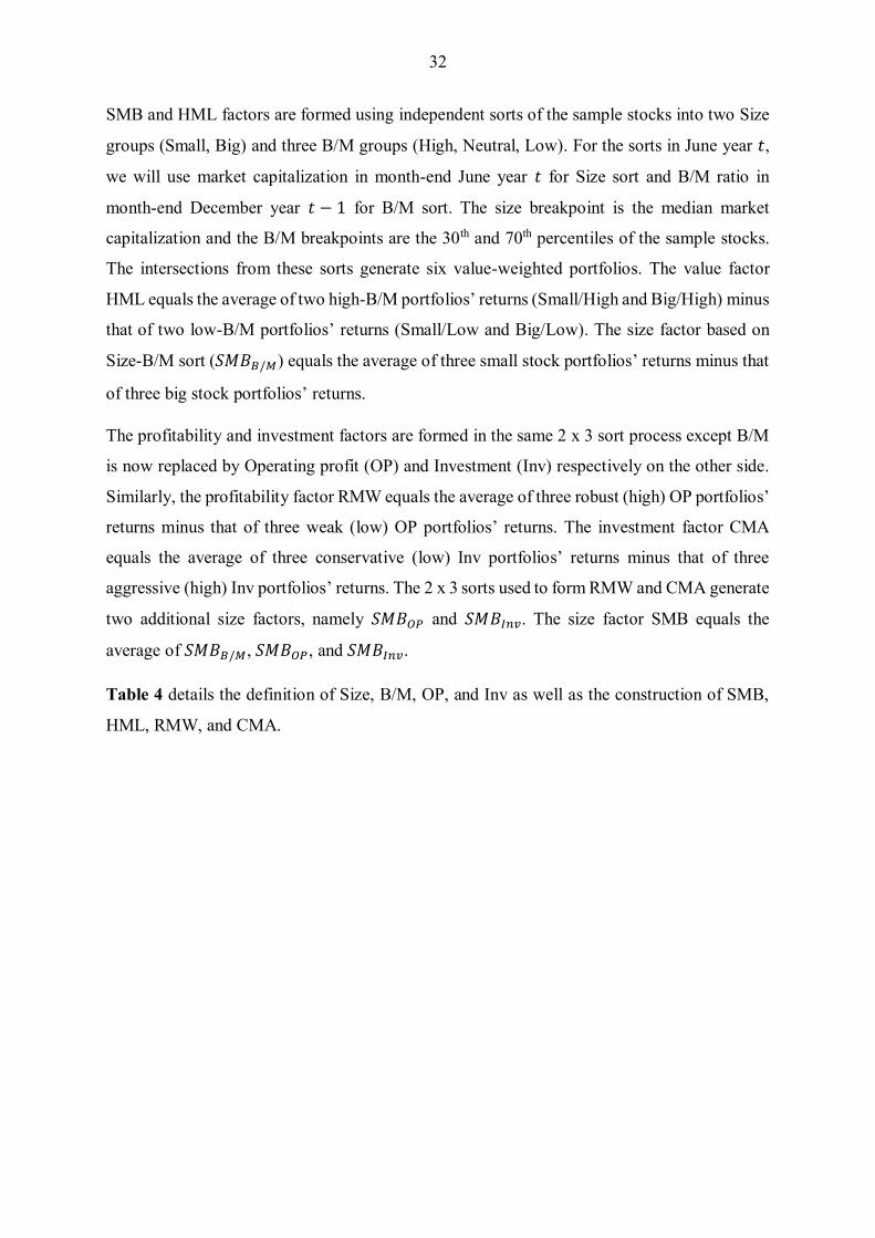
32

SMB and HML factors are formed using independent sorts of the sample stocks into two Size

groups (Small, Big) and three B/M groups (High, Neutral, Low). For the sorts in June year 𝑡,

we will use market capitalization in month-end June year 𝑡 for Size sort and B/M ratio in

month-end December year 𝑡 − 1 for B/M sort. The size breakpoint is the median market

capitalization and the B/M breakpoints are the 30th and 70th percentiles of the sample stocks.

The intersections from these sorts generate six value-weighted portfolios. The value factor

HML equals the average of two high-B/M portfolios’ returns (Small/High and Big/High) minus

that of two low-B/M portfolios’ returns (Small/Low and Big/Low). The size factor based on

Size-B/M sort (𝑆𝑀𝐵𝐵/𝑀) equals the average of three small stock portfolios’ returns minus that

of three big stock portfolios’ returns.

The profitability and investment factors are formed in the same 2 x 3 sort process except B/M

is now replaced by Operating profit (OP) and Investment (Inv) respectively on the other side.

Similarly, the profitability factor RMW equals the average of three robust (high) OP portfolios’

returns minus that of three weak (low) OP portfolios’ returns. The investment factor CMA

equals the average of three conservative (low) Inv portfolios’ returns minus that of three

aggressive (high) Inv portfolios’ returns. The 2 x 3 sorts used to form RMW and CMA generate

two additional size factors, namely 𝑆𝑀𝐵𝑂𝑃 and 𝑆𝑀𝐵𝐼𝑛𝑣. The size factor SMB equals the

average of 𝑆𝑀𝐵𝐵/𝑀, 𝑆𝑀𝐵𝑂𝑃, and 𝑆𝑀𝐵𝐼𝑛𝑣.

Table 4 details the definition of Size, B/M, OP, and Inv as well as the construction of SMB,

HML, RMW, and CMA.

33

Table 4 Sort process and construction of SMB, HML, RMW, and CMA.

Independent sorts are used to assign stocks to two Size groups and three B/M, OP, and Inv groups. The intersections of

Size groups and the other groups define double-sorted portfolios used to construct the factors. These portfolios are labeled

with two letters. The first letter always describes the size groups: Small (S) or Big (B). The second letter describes the

B/M groups: High (H), Neutral (N), or Low (L); the OP groups: Robust (R), Neutral (N), or Weak (W); or the Inv groups:

Conservative (C), Neutral (N), or Aggressive (A). For example, SH portfolio comprises Small (S) stocks with and High

(H) B/M.

Sort criteria and breakpoints

(sort in June year t) Factor construction

Size sorted by: 𝑴𝒂𝒓𝒌𝒆𝒕 𝒄𝒂𝒑 𝒕 (month-end June year t)

Size breakpoint: sample median

𝑆𝑀𝐵𝐵/𝑀 = (𝑆𝐻 + 𝑆𝑁 + 𝑆𝐿)/3 − (𝐵𝐻 + 𝐵𝑁 + 𝐵𝐿)/3

𝑆𝑀𝐵𝑂𝑃 = (𝑆𝑅 + 𝑆𝑁 + 𝑆𝑊)/3 − (𝐵𝑅 + 𝐵𝑁 + 𝐵𝑊)/3

𝑆𝑀𝐵𝐼𝑛𝑣 = (𝑆𝐶 + 𝑆𝑁 + 𝑆𝐴)/3 − (𝐵𝐶 + 𝐵𝑁 + 𝐵𝐴)/3

𝑺𝑴𝑩 = (𝑺𝑴𝑩𝑩/𝑴 + 𝑺𝑴𝑩𝑶𝑷 + 𝑺𝑴𝑩𝑰𝒏𝒗)/𝟑

Value sorted by:

𝑩/𝑴𝒕−𝟏 =𝑩𝒐𝒐𝒌 − 𝒆𝒒𝒖𝒊𝒕𝒚𝒕−𝟏

𝑴𝒂𝒓𝒌𝒆𝒕 𝒄𝒂𝒑 𝒕−𝟏

Value breakpoints: 30th and 70th percentiles

𝑯𝑴𝑳 = (𝑺𝑯 + 𝑩𝑯)/𝟐 – (𝑺𝑳 + 𝑩𝑳)/𝟐

Profitability sorted by:

𝑶𝑷𝒕−𝟏 =𝑹𝒆𝒗𝒕−𝟏 − 𝑪𝑶𝑮𝑺𝒕−𝟏 − 𝑺𝑮&𝑨𝒕−𝟏 − 𝑰𝒏𝒕𝒆𝒓𝒆𝒔𝒕 𝒕−𝟏

𝑩𝒐𝒐𝒌 − 𝒆𝒒𝒖𝒊𝒕𝒚 𝒕−𝟏

Profitability breakpoints: 30th and 70th percentiles

𝑹𝑴𝑾 = (𝑺𝑹 + 𝑩𝑹)/𝟐 – (𝑺𝑾 + 𝑩𝑾)/2

Investment sorted by:

𝑰𝒏𝒗𝒕−𝟏 =𝑻𝒐𝒕𝒂𝒍 𝑨𝒔𝒔𝒆𝒕𝒔𝒕−𝟏 − 𝑻𝒐𝒕𝒂𝒍 𝑨𝒔𝒔𝒆𝒕𝒔𝒕−𝟐

𝑻𝒐𝒕𝒂𝒍 𝑨𝒔𝒔𝒆𝒕𝒔𝒕−𝟐

Investment breakpoints: 30th and 70th percentiles

𝑪𝑴𝑨 = (𝑺𝑪 + 𝑩𝑪)/𝟐 – (𝑺𝑨 + 𝑩𝑨)/𝟐

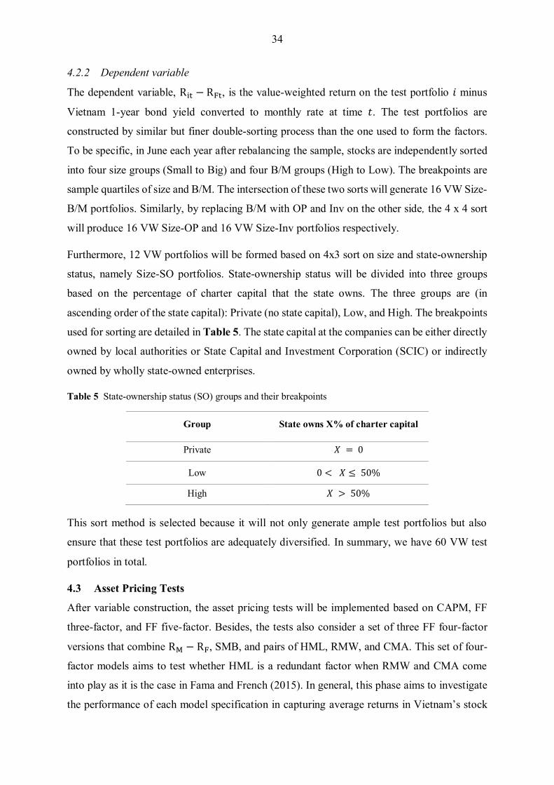
34

4.2.2 Dependent variable

The dependent variable, Rit − RFt, is the value-weighted return on the test portfolio 𝑖 minus

Vietnam 1-year bond yield converted to monthly rate at time 𝑡. The test portfolios are

constructed by similar but finer double-sorting process than the one used to form the factors.

To be specific, in June each year after rebalancing the sample, stocks are independently sorted

into four size groups (Small to Big) and four B/M groups (High to Low). The breakpoints are

sample quartiles of size and B/M. The intersection of these two sorts will generate 16 VW Size-

B/M portfolios. Similarly, by replacing B/M with OP and Inv on the other side, the 4 x 4 sort

will produce 16 VW Size-OP and 16 VW Size-Inv portfolios respectively.

Furthermore, 12 VW portfolios will be formed based on 4x3 sort on size and state-ownership

status, namely Size-SO portfolios. State-ownership status will be divided into three groups

based on the percentage of charter capital that the state owns. The three groups are (in

ascending order of the state capital): Private (no state capital), Low, and High. The breakpoints

used for sorting are detailed in Table 5. The state capital at the companies can be either directly

owned by local authorities or State Capital and Investment Corporation (SCIC) or indirectly

owned by wholly state-owned enterprises.

Table 5 State-ownership status (SO) groups and their breakpoints

Group State owns X% of charter capital

Private 𝑋 = 0

Low 0 < 𝑋 ≤ 50%

High 𝑋 > 50%

This sort method is selected because it will not only generate ample test portfolios but also

ensure that these test portfolios are adequately diversified. In summary, we have 60 VW test

portfolios in total.

4.3 Asset Pricing Tests

After variable construction, the asset pricing tests will be implemented based on CAPM, FF

three-factor, and FF five-factor. Besides, the tests also consider a set of three FF four-factor

versions that combine RM − RF, SMB, and pairs of HML, RMW, and CMA. This set of four-

factor models aims to test whether HML is a redundant factor when RMW and CMA come

into play as it is the case in Fama and French (2015). In general, this phase aims to investigate

the performance of each model specification in capturing average returns in Vietnam’s stock

35

market. The regressions will be conducted using ordinary least squares (OLS) method.

Specifications of asset pricing tests are detailed in Table 6.

Table 6 Specifications of Asset Pricing Tests

Rm-Rf is the value-weighted return on the market portfolio of all sample stocks minus Vietnam 1-year

government bond yield converted to monthly basis; SMB (small-minus-big) is the size factor; HML (high-

minus-low) is the value factor; RMW (robust-minus-weak) is the profitability factor; and CMA

(conservative-minus-aggressive) is the investment factor. All the factors (except Rm-Rf) are constructed

from independent sorts of stocks into two Size groups and three B/M groups, three OP groups, or three Inv

groups.

Model Regression equation

Capital Asset Pricing

Model 𝑅𝑖𝑡 − 𝑅𝐹𝑡 = 𝑎𝑖 + 𝑏𝑖(𝑅𝑀𝑡 − 𝑅𝐹𝑡) + 𝑒𝑖𝑡

Fama – French Three-

Factor Model 𝑅𝑖𝑡 − 𝑅𝐹𝑡 = 𝑎𝑖 + 𝑏𝑖(𝑅𝑀𝑡 − 𝑅𝐹𝑡) + 𝑠𝑖𝑆𝑀𝐵𝑡 + ℎ𝑖𝐻𝑀𝐿𝑡 + 𝑒𝑖𝑡

Fama – French Five-

Factor Model 𝑅𝑖𝑡 − 𝑅𝐹𝑡 = 𝑎𝑖 + 𝑏𝑖(𝑅𝑀𝑡 − 𝑅𝐹𝑡) + 𝑠𝑖𝑆𝑀𝐵𝑡 + ℎ𝑖𝐻𝑀𝐿𝑡 + 𝑟𝑖𝑅𝑀𝑊𝑡 + 𝑐𝑖𝐶𝑀𝐴𝑡 + 𝑒𝑖𝑡

Fama – French Four-

Factor (combine 𝐑𝐌 −

𝐑𝐅, SMB, and pairs of

HML, RMW, and

CMA)

(1) 𝑅𝑖𝑡 − 𝑅𝐹𝑡 = 𝑎𝑖 + 𝑏𝑖(𝑅𝑀𝑡 − 𝑅𝐹𝑡) + 𝑠𝑖𝑆𝑀𝐵𝑡 + ℎ𝑖𝐻𝑀𝐿𝑡 + 𝑟𝑖𝑅𝑀𝑊𝑡 + 𝑒𝑖𝑡

(2) 𝑅𝑖𝑡 − 𝑅𝐹𝑡 = 𝑎𝑖 + 𝑏𝑖(𝑅𝑀𝑡 − 𝑅𝐹𝑡) + 𝑠𝑖𝑆𝑀𝐵𝑡 + ℎ𝑖𝐻𝑀𝐿𝑡 + 𝑐𝑖𝐶𝑀𝐴𝑡 + 𝑒𝑖𝑡

(3) 𝑅𝑖𝑡 − 𝑅𝐹𝑡 = 𝑎𝑖 + 𝑏𝑖(𝑅𝑀𝑡 − 𝑅𝐹𝑡) + 𝑠𝑖𝑆𝑀𝐵𝑡 + 𝑟𝑖𝑅𝑀𝑊𝑡 + 𝑐𝑖𝐶𝑀𝐴𝑡 + 𝑒𝑖𝑡

4.4 Factor Spanning Tests

The factor spanning tests will help to determine whether any factor in the FF five-factor model

can be fully explained by other factors regarding Vietnam’s stock market. Specifically, the tests

will regress each of the five factors on the other four by using OLS method. Specifications of

factor spanning tests are detailed in Table 7.

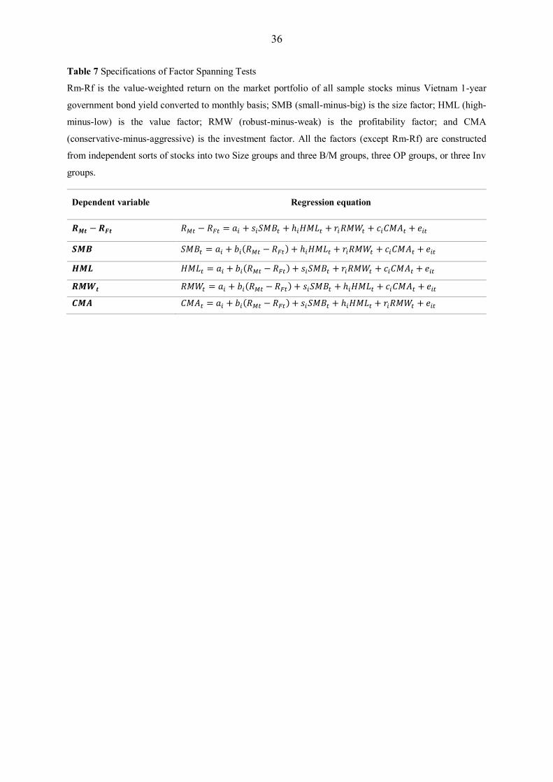
36

Table 7 Specifications of Factor Spanning Tests






groups.

Dependent variable Regression equation

𝑹𝑴𝒕 − 𝑹𝑭𝒕 𝑅𝑀𝑡 − 𝑅𝐹𝑡 = 𝑎𝑖 + 𝑠𝑖𝑆𝑀𝐵𝑡 + ℎ𝑖𝐻𝑀𝐿𝑡 + 𝑟𝑖𝑅𝑀𝑊𝑡 + 𝑐𝑖𝐶𝑀𝐴𝑡 + 𝑒𝑖𝑡

𝑺𝑴𝑩 𝑆𝑀𝐵𝑡 = 𝑎𝑖 + 𝑏𝑖(𝑅𝑀𝑡 − 𝑅𝐹𝑡) + ℎ𝑖𝐻𝑀𝐿𝑡 + 𝑟𝑖𝑅𝑀𝑊𝑡 + 𝑐𝑖𝐶𝑀𝐴𝑡 + 𝑒𝑖𝑡

𝑯𝑴𝑳 𝐻𝑀𝐿𝑡 = 𝑎𝑖 + 𝑏𝑖(𝑅𝑀𝑡 − 𝑅𝐹𝑡) + 𝑠𝑖𝑆𝑀𝐵𝑡 + 𝑟𝑖𝑅𝑀𝑊𝑡 + 𝑐𝑖𝐶𝑀𝐴𝑡 + 𝑒𝑖𝑡

𝑹𝑴𝑾𝒕 𝑅𝑀𝑊𝑡 = 𝑎𝑖 + 𝑏𝑖(𝑅𝑀𝑡 − 𝑅𝐹𝑡) + 𝑠𝑖𝑆𝑀𝐵𝑡 + ℎ𝑖𝐻𝑀𝐿𝑡 + 𝑐𝑖𝐶𝑀𝐴𝑡 + 𝑒𝑖𝑡

𝑪𝑴𝑨 𝐶𝑀𝐴𝑡 = 𝑎𝑖 + 𝑏𝑖(𝑅𝑀𝑡 − 𝑅𝐹𝑡) + 𝑠𝑖𝑆𝑀𝐵𝑡 + ℎ𝑖𝐻𝑀𝐿𝑡 + 𝑟𝑖𝑅𝑀𝑊𝑡 + 𝑒𝑖𝑡

37

5 FINDINGS AND DISCUSSION

The findings and discussion part begins with Section 5.1 – “The Playing Field”, which

examines the patterns in average returns as well as in book-to-market, operating profitability,

and investment. Subsequently, Section 5.2 and 5.3 respectively present summary statistics of

factor returns and correlations among different factors. Section 5.4 continues with findings

from the primary task of the thesis - testing how well different asset pricing models explain

average returns in Vietnam’ stock market. Finally, Section 5.5 shows factor spanning test

results and discusses which factor is redundant.

5.1 The Playing Field

This thesis aims to investigate the capability of the FF five-factor model and models that

include subsets of its factors in explaining variation in Vietnam stock returns. Before discussing

the regression results, we will examine the patterns in average returns as well as in B/M, OP,

and Inv of 60 VW test portfolios. Patterns in average returns are usually referred to as effects.

For instance, size effect is the size pattern in average returns. Section 5.1.1 to 5.1.5 will discuss

the five effects: size, value, profitability, investment, and state-ownership status. Section 5.1.6

will discuss other patterns in B/M, OP, and Inv. Table 8 shows time-series averages of monthly

excess returns, B/M, OP, and Inv of 60 VW test portfolios.

It is important to note that this section only discusses univariate characteristics. Therefore,

interpretation in this section should be taken with caution as univariate characteristics can differ

from multivariate regression slopes, which estimate marginal effects holding other explanatory

variables constant (Fama and French, 2015). However, it is interesting to see whether factor

slopes line up with these univariate characteristics.

5.1.1 Size Effect

For 16 VW Size-B/M portfolios, the size effect is not obvious as average returns do not

typically fall from small stocks to big stocks. That is, average return pattern from small to big

stocks varies across different B/M groups. For example, in the lowest B/M column, stocks in

the 3rd size group have the lowest average return. However, in the highest B/M column, stocks

in this size group have the second highest average return. Although average returns do not

monotonously decrease from small to big stocks for our 16 VW Size-B/M portfolios, the

smallest size portfolios almost always earn the highest average return (with the exception in

2nd B/M group). Thus, size effect still occurs to a weak extent for Size-B/M portfolios.

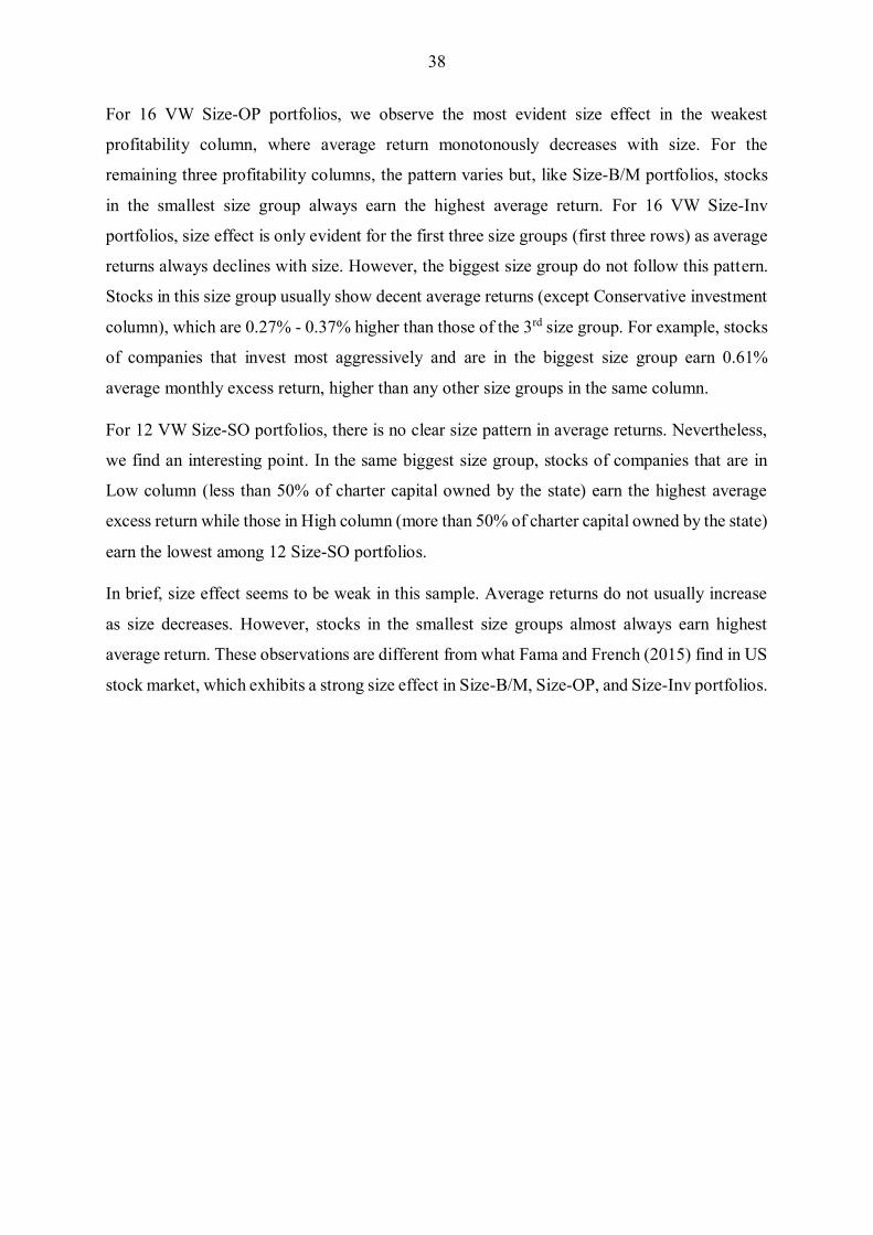
38

For 16 VW Size-OP portfolios, we observe the most evident size effect in the weakest

profitability column, where average return monotonously decreases with size. For the

remaining three profitability columns, the pattern varies but, like Size-B/M portfolios, stocks

in the smallest size group always earn the highest average return. For 16 VW Size-Inv

portfolios, size effect is only evident for the first three size groups (first three rows) as average

returns always declines with size. However, the biggest size group do not follow this pattern.

Stocks in this size group usually show decent average returns (except Conservative investment

column), which are 0.27% - 0.37% higher than those of the 3rd size group. For example, stocks

of companies that invest most aggressively and are in the biggest size group earn 0.61%

average monthly excess return, higher than any other size groups in the same column.

For 12 VW Size-SO portfolios, there is no clear size pattern in average returns. Nevertheless,

we find an interesting point. In the same biggest size group, stocks of companies that are in

Low column (less than 50% of charter capital owned by the state) earn the highest average

excess return while those in High column (more than 50% of charter capital owned by the state)

earn the lowest among 12 Size-SO portfolios.

In brief, size effect seems to be weak in this sample. Average returns do not usually increase

as size decreases. However, stocks in the smallest size groups almost always earn highest

average return. These observations are different from what Fama and French (2015) find in US

stock market, which exhibits a strong size effect in Size-B/M, Size-OP, and Size-Inv portfolios.

39

Table 8 Time-series averages of excess returns, B/M, OP, and Inv of 60 VW test portfolios formed on Size and B/M, OP, Inv, or SO;

July 2009 - December 2017, 102 months.

The table rows always refer to size quartiles while the table columns refer to B/M, profitability, investment, and state-ownership

groups. Both rows and columns are in ascending order; for Size: Small to Big; for B/M: Low to High; for OP: Weak to Robust; for

Inv: Conservative (Cons.) to Aggressive (Aggr.); and for SO: Private (Priv.) to High. The intersections of rows and columns form

double-sorted portfolios. Panel A presents average excess return of 60 VW test portfolios; monthly excess return is equal to monthly

return minus Vietnam 1-year government bond yield converted to monthly basis. Panel B presents average B/M of 60 VW test

portfolios; B/M is equal to book equity divided by market capitalization. Panel C presents average OP; OP is equal to revenue minus

COGS, SG&A, and interest expense, all divided by book equity. Panel D presents average Inv; Inv is equal to total asset growth rate.

Book-to-Market (B/M) Profitability (OP) Investment (Inv) State-ownership (SO)

Low 2 3 High Weak 2 3 Robust Cons. 2 3 Aggr. Priv. Low High

Panel A: Excess return

Small 0.86 0.66 1.03 0.79 1.05 0.46 0.39 1.26 0.76 0.91 0.72 0.59 1.02 0.23 0.28

2 -0.01 0.82 0.44 0.01 0.06 0.12 0.70 0.60 0.20 0.44 0.35 0.23 0.47 -0.10 0.09

3 -0.19 -0.06 0.14 0.74 0.01 0.01 0.04 0.15 -0.05 0.12 -0.07 -0.24 -0.01 0.31 -0.09

Big 0.53 0.06 0.28 0.16 -0.70 0.23 0.10 0.64 -0.24 0.48 0.20 0.61 0.49 1.36 -0.32

Panel B: Book-to-Market (B/M)

Small 0.66 1.07 1.51 2.72 2.27 1.97 1.52 1.38 2.00 1.87 1.77 1.84 1.95 1.71 2.05

2 0.62 1.02 1.53 2.51 2.00 1.65 1.36 1.23 1.62 1.75 1.51 1.46 1.66 1.39 1.46

3 0.59 1.02 1.53 2.42 1.83 1.34 1.09 0.92 1.35 1.31 1.18 1.13 1.27 1.10 1.25

Big 0.56 1.01 1.43 2.36 1.36 1.10 0.98 0.68 1.12 1.11 0.93 0.86 0.98 0.90 1.01

Panel C: Profitability (OP)

Small 0.24 0.16 0.16 0.08 -0.06 0.12 0.23 0.46 0.07 0.13 0.20 0.19 0.13 0.14 0.13

2 0.18 0.22 0.16 0.12 -0.07 0.13 0.23 0.48 0.10 0.16 0.21 0.21 0.14 0.18 0.25

3 0.32 0.24 0.18 0.13 -0.02 0.13 0.23 0.50 0.18 0.24 0.25 0.27 0.19 0.21 0.38

Big 0.28 0.19 0.16 0.10 -0.06 0.12 0.24 0.43 0.14 0.22 0.25 0.24 0.18 0.26 0.29

Panel D: Investment (Inv)

Small 0.04 0.14 0.10 0.07 0.05 0.08 0.15 0.15 -0.12 0.04 0.16 0.57 0.12 0.07 0.07

2 0.17 0.14 0.14 0.09 0.11 0.17 0.14 0.15 -0.11 0.04 0.16 0.54 0.15 0.13 0.11

3 0.24 0.15 0.16 0.10 0.18 0.20 0.15 0.17 -0.10 0.04 0.15 0.57 0.20 0.13 0.13

Big 0.27 0.22 0.19 0.11 0.30 0.26 0.20 0.22 -0.09 0.04 0.15 0.59 0.30 0.18 0.13

40

5.1.2 Value Effect

Value effect, the relation between B/M and average returns, is not evident in 16 VW Size-B/M

portfolios. If value effect takes place, average return should increase with B/M in each size

group. In these Size-B/M portfolios, only stocks in the 3rd size group exhibit a strong value

effect as average return increases monotonously with B/M. However, other size groups seem

to display a reverse value effect as average return decrease with B/M. Specifically, stocks in

the highest B/M group earn the second lowest average returns in the remaining three size

groups. This finding is in contradiction to what Fama and French (2015) observe.

5.1.3 Profitability Effect

Profitability effect, the relation between OP and average returns, is intuitive in a sense that

stocks of companies with robust profit should earn higher average return than those with weak

profit. This effect seems to reflect in our 16 VW Size-OP portfolios. Although the effect is not

smooth, Weak OP column tends to have lower average returns than the Robust one.

Furthermore, stocks in the Robust column almost always gain the highest average returns –

three out of four size groups. Nevertheless, there exists a glaring outlier in Small-Weak

portfolio, which earns the second highest average return among all Size-OP portfolios, only

lower than that of the Small-Robust stocks.

5.1.4 Investment Effect

In Fama and French’s sample (2015), stocks of companies that invest aggressively tend to have

lower average returns than those with conservative investment level, measured by lagged asset

growth. This negative relationship between investment and average stock return is also implied

in the Miller Modigliani valuation formula (Equation 8). However, this pattern is not

consistent in our sample and reversal happens in some instances. For example, stocks in the 2nd

investment quartile tend to have the largest average return (three out of four size groups) while

those in the 1st investment quartile, the most conservative, have the lowest average return in

two out of four size groups. In the biggest size group, average return even monotonously

increases with investment. In this size group, stocks of companies in the 4th investment quartile,

the most aggressive, earn the highest average monthly excess return of 0.61% – a wide spread

of 0.85% with the 1st investment quartile.

5.1.5 State-ownership Effect

State-ownership effect will be examined in 12 VW Size-SO portfolios. Like some effects

discussed above, state-ownership pattern in average returns is not consistent and varies across

41

size groups. In the 1st and 2nd size quartile, stocks of private companies earn the highest average

return while those of low-state-capital companies earn the lowest. However, this pattern

reverses in the 3rd and 4th size quartile, where stocks in the low-state-capital group gain the

highest average return. As for stocks of high-state-capital companies, they usually have

relatively low average return across all size quartiles.

5.1.6 Other Patterns

There exists a strong pattern between B/M and OP: lower B/M tends to associate with higher

OP and vice versa. For example, in 16 VW Size-BM portfolios, OP gradually decreases as B/M

increases from the 1st to the 4th quartile in nearly all size groups except the second one. In the

second size group, the trend is not smooth but it persists. This negative relation between OP

and B/M can be observed in both Size-OP and Size-B/M portfolios. That is, profitability pattern

in B/M (Table 8 Panel B of Size-OP portfolios) is equivalent to B/M pattern in profitability

(Table 8 Panel C of Size-B/M portfolios). Investment also exhibits a negative relation with

B/M in that more aggressive investment level usually comes with lower B/M, which is reflected

in both Size-Inv and Size-B/M portfolios.

Unlike the previous two relations, the relation between profitability and investment is not

straightforward. While profitability pattern in investment is not clear (Table 8 Panel D of Size-

OP portfolios), investment pattern in profitability seems to be strong (Table 8 Panel C of Size-

Inv portfolios). For 16 VW Size-Inv portfolios, companies that invest more aggressively tend

to have more robust profitability. All these observations on the relations between B/M, OP,

and Inv are consistent with what Fama and French (2015) find in their US sample.

When examining 12 VW Size-SO portfolios, we find no evident pattern between ownership

status and B/M. However, when it comes to profitability and investment, companies that have

state capital tend to have more robust profitability but lower investment level than private ones.

Nguyen et al. (2015), on the other hand, find that private companies tend to have higher B/M,

stronger profitability, and more aggressive investment level. This disparity can be attributed to

difference in state-ownership classfication, data source, and test period.

5.2 Summary Statistics for Factor Returns

Table 9 presents the summary statistics for each factor. The range (max minus min) and

standard deviation of these factors do not differ significantly from one another except for CMA,

which has the smallest range and standard deviation. Among all the five factors, RMW has

42

the highest average return of 0.738% per month. This phenomenon is consistent with our

previous univariate analysis that there is a strong profitability effect in the sample.

Table 9 Summary Statistics for Factor Returns; July 2009 - December 2017, 102 months

This table presents time-series mean, median, standard deviation, min, and max of different factor percent

returns. Rm-Rf is the value-weighted return on the market portfolio of all sample stocks minus Vietnam 1-

year government bond yield converted to monthly basis; SMB (small-minus-big) is the size factor; HML

(high-minus-low) is the value factor; RMW (robust-minus-weak) is the profitability factor; and CMA



groups.

Mean Median SD Min Max

RM − RF 0.306 0.747 5.131 -14.00 12.83

SMB 0.174 0.162 4.200 -11.74 14.44

HML 0.060 -0.905 4.852 -10.00 14.04

RMW 0.738 1.266 4.161 -10.88 10.69

CMA -0.126 -0.247 2.664 -6.31 7.53

Other FF factors (SMB, HML, and CMA) show a relatively low average return over the test

period. For example, HML shows a close-to-zero average return of 0.06% per month, meaning

there is little difference in return between low and high B/M stocks on average. CMA, on the

other hand, even exhibits a negative monthly average return of -0.126%. This negative number

indicates that stocks of companies that invest aggressively on average perform better than those

with conservative investment level, which differs from with what Fama and French (2015) find

in US stock market. Besides the summary statistics table, we can also study the behavior of

different factors through their cumulative returns over the test period (Figure 5).

43

Figure 5 Cumulative returns of the market and four Fama-French factors (profit reinvested); July 2009 -

December 2017, 102 months in total

Among the four FF factors, RMW has the highest cumulative return over the test period, which

is above the market cumulative return most of the time. At the end of December 2017, RMW

cumulative return is approximately 94%.

During the test period, SMB cumulative return reached its highest point of 42.4% in June 2010

and then began to decline to below zero until gaining back since September 2014. However,

this factor cumulative return started to plunge again in October 2017, ending the test period

with only 9.3%.

The cumulative return of HML exhibits a generally similar pattern to that of SMB until March

2015 when the two lines diverged. HML cumulative return ends the period below zero at -5.4%

with the lowest point at -30.4% in July 2013.

Among all factors, CMA has the lowest cumulative return as it always stays below zero

throughout the test period. This phenomenon provides evidence that stocks of companies with

aggressive investment tend to perform better than those with conservative investment. If CMA

is called investment premium, this means that investment premium is negative in Vietnam

stock market, at least during this test period.

-60%

-40%

-20%

0%

20%

40%

60%

80%

100%

120%

140%hei

nä.

09

mar

ras.

09

maa

lis.

10

hei

nä.

10

mar

ras.

10

maa

lis.

11

hei

nä.

11

mar

ras.

11

maa

lis.

12

hei

nä.

12

mar

ras.

12

maa

lis.

13

hei

nä.

13

mar

ras.

13

maa

lis.

14

hei

nä.

14

mar

ras.

14

maa

lis.

15

hei

nä.

15

mar

ras.

15

maa

lis.

16

hei

nä.

16

mar

ras.

16

maa

lis.

17

hei

nä.

17

mar

ras.

17

Cumulative Returns Jul 09 - Dec 17

Rm SMB HML RMW CMA

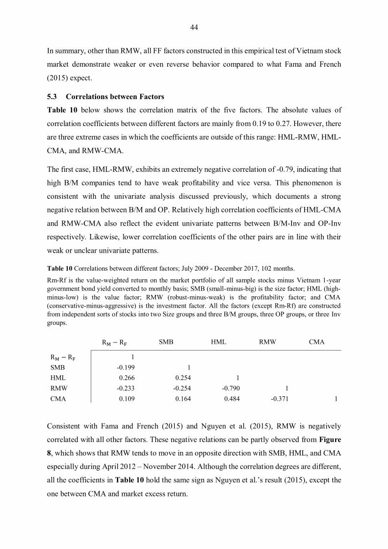
44

In summary, other than RMW, all FF factors constructed in this empirical test of Vietnam stock

market demonstrate weaker or even reverse behavior compared to what Fama and French

(2015) expect.

5.3 Correlations between Factors

Table 10 below shows the correlation matrix of the five factors. The absolute values of

correlation coefficients between different factors are mainly from 0.19 to 0.27. However, there

are three extreme cases in which the coefficients are outside of this range: HML-RMW, HML-

CMA, and RMW-CMA.

The first case, HML-RMW, exhibits an extremely negative correlation of -0.79, indicating that

high B/M companies tend to have weak profitability and vice versa. This phenomenon is

consistent with the univariate analysis discussed previously, which documents a strong

negative relation between B/M and OP. Relatively high correlation coefficients of HML-CMA

and RMW-CMA also reflect the evident univariate patterns between B/M-Inv and OP-Inv

respectively. Likewise, lower correlation coefficients of the other pairs are in line with their

weak or unclear univariate patterns.

Table 10 Correlations between different factors; July 2009 - December 2017, 102 months.






groups.

RM − RF SMB HML RMW CMA

RM − RF 1

SMB -0.199 1

HML 0.266 0.254 1

RMW -0.233 -0.254 -0.790 1

CMA 0.109 0.164 0.484 -0.371 1

Consistent with Fama and French (2015) and Nguyen et al. (2015), RMW is negatively

correlated with all other factors. These negative relations can be partly observed from Figure

8, which shows that RMW tends to move in an opposite direction with SMB, HML, and CMA

especially during April 2012 – November 2014. Although the correlation degrees are different,

all the coefficients in Table 10 hold the same sign as Nguyen et al.’s result (2015), except the

one between CMA and market excess return.

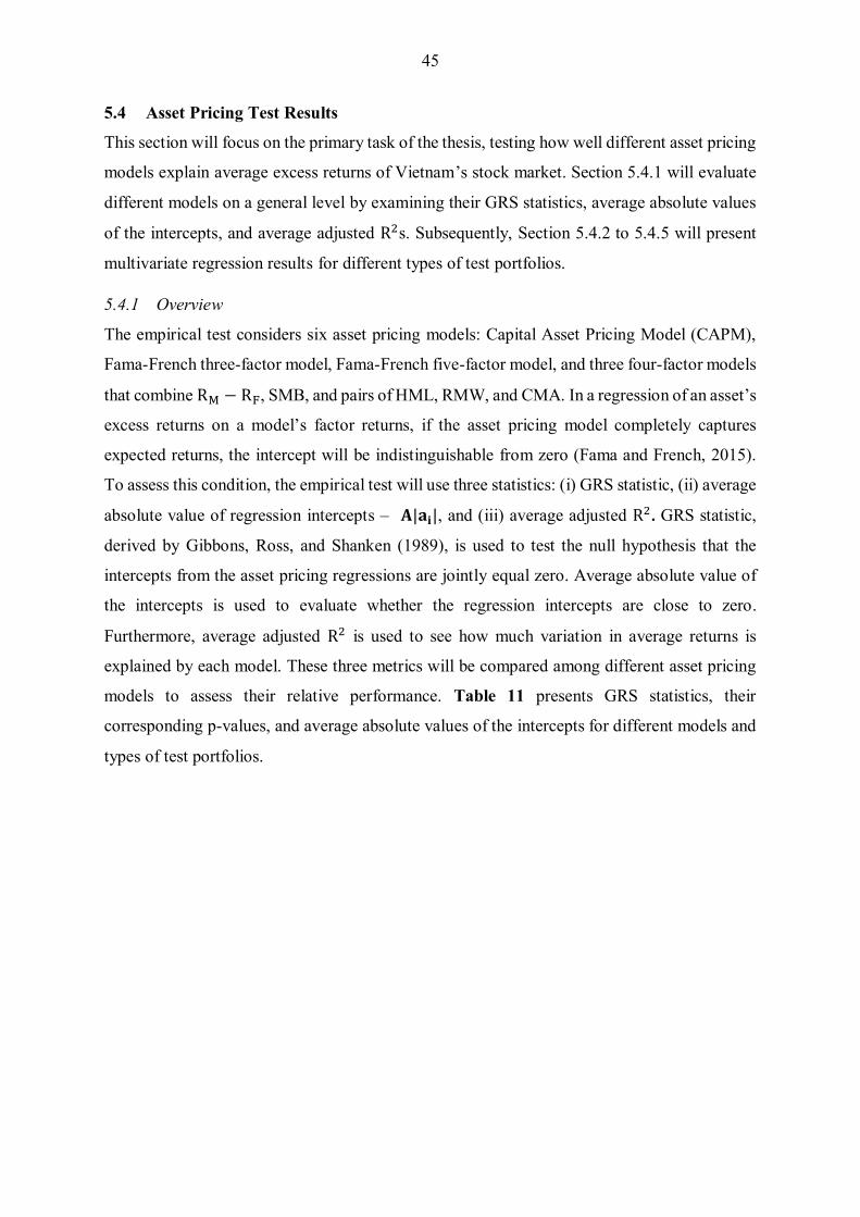
45

5.4 Asset Pricing Test Results

This section will focus on the primary task of the thesis, testing how well different asset pricing

models explain average excess returns of Vietnam’s stock market. Section 5.4.1 will evaluate

different models on a general level by examining their GRS statistics, average absolute values

of the intercepts, and average adjusted R2s. Subsequently, Section 5.4.2 to 5.4.5 will present

multivariate regression results for different types of test portfolios.

5.4.1 Overview

The empirical test considers six asset pricing models: Capital Asset Pricing Model (CAPM),

Fama-French three-factor model, Fama-French five-factor model, and three four-factor models

that combine RM − RF, SMB, and pairs of HML, RMW, and CMA. In a regression of an asset’s

excess returns on a model’s factor returns, if the asset pricing model completely captures

expected returns, the intercept will be indistinguishable from zero (Fama and French, 2015).

To assess this condition, the empirical test will use three statistics: (i) GRS statistic, (ii) average

absolute value of regression intercepts – 𝐀|𝐚𝐢|, and (iii) average adjusted R2. GRS statistic,

derived by Gibbons, Ross, and Shanken (1989), is used to test the null hypothesis that the

intercepts from the asset pricing regressions are jointly equal zero. Average absolute value of

the intercepts is used to evaluate whether the regression intercepts are close to zero.

Furthermore, average adjusted R2 is used to see how much variation in average returns is

explained by each model. These three metrics will be compared among different asset pricing

models to assess their relative performance. Table 11 presents GRS statistics, their

corresponding p-values, and average absolute values of the intercepts for different models and

types of test portfolios.

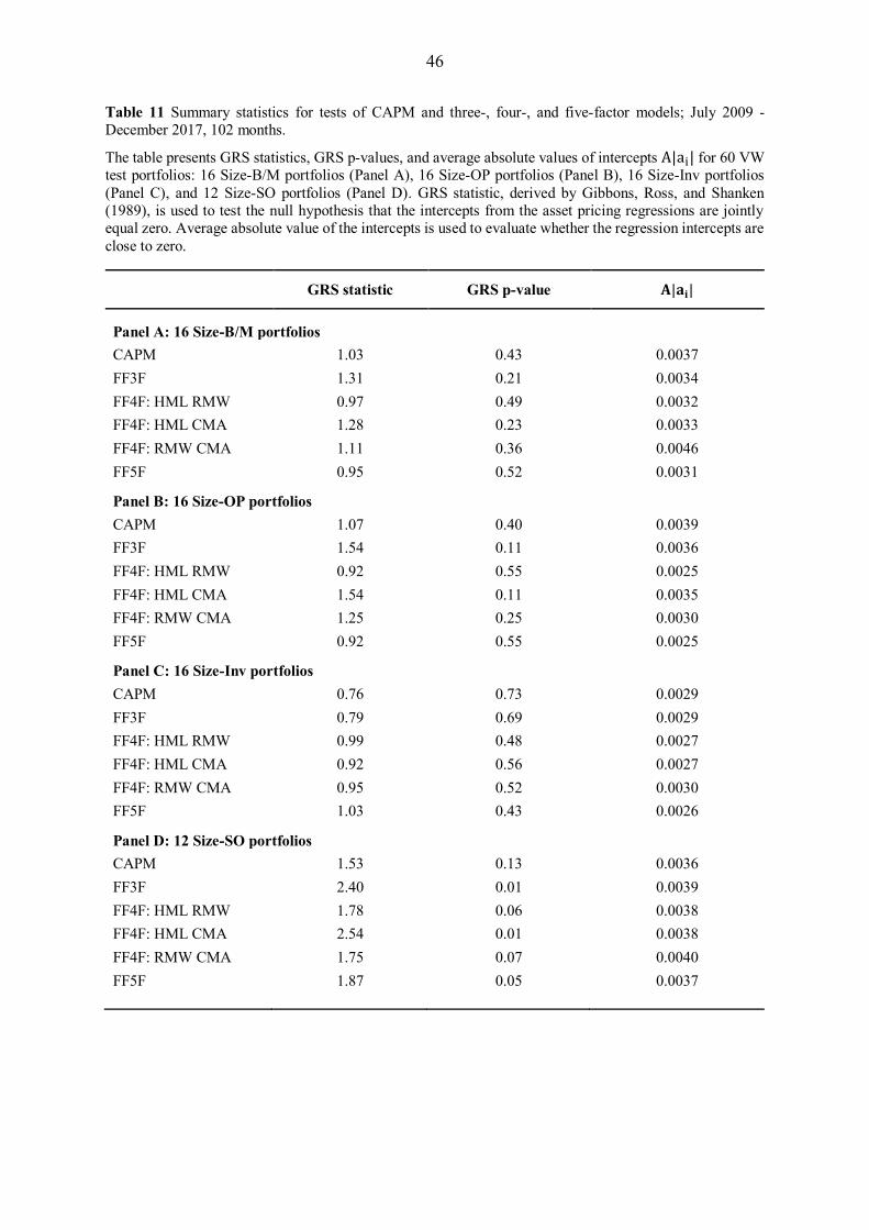
46

Table 11 Summary statistics for tests of CAPM and three-, four-, and five-factor models; July 2009 -

December 2017, 102 months.

The table presents GRS statistics, GRS p-values, and average absolute values of intercepts A|ai| for 60 VW

test portfolios: 16 Size-B/M portfolios (Panel A), 16 Size-OP portfolios (Panel B), 16 Size-Inv portfolios

(Panel C), and 12 Size-SO portfolios (Panel D). GRS statistic, derived by Gibbons, Ross, and Shanken

(1989), is used to test the null hypothesis that the intercepts from the asset pricing regressions are jointly

equal zero. Average absolute value of the intercepts is used to evaluate whether the regression intercepts are

close to zero.

GRS statistic GRS p-value 𝐀|𝐚𝐢|

Panel A: 16 Size-B/M portfolios

CAPM 1.03 0.43 0.0037

FF3F 1.31 0.21 0.0034

FF4F: HML RMW 0.97 0.49 0.0032

FF4F: HML CMA 1.28 0.23 0.0033

FF4F: RMW CMA 1.11 0.36 0.0046

FF5F 0.95 0.52 0.0031

Panel B: 16 Size-OP portfolios

CAPM 1.07 0.40 0.0039

FF3F 1.54 0.11 0.0036

FF4F: HML RMW 0.92 0.55 0.0025

FF4F: HML CMA 1.54 0.11 0.0035

FF4F: RMW CMA 1.25 0.25 0.0030

FF5F 0.92 0.55 0.0025

Panel C: 16 Size-Inv portfolios

CAPM 0.76 0.73 0.0029

FF3F 0.79 0.69 0.0029

FF4F: HML RMW 0.99 0.48 0.0027

FF4F: HML CMA 0.92 0.56 0.0027

FF4F: RMW CMA 0.95 0.52 0.0030

FF5F 1.03 0.43 0.0026

Panel D: 12 Size-SO portfolios

CAPM 1.53 0.13 0.0036

FF3F 2.40 0.01 0.0039

FF4F: HML RMW 1.78 0.06 0.0038

FF4F: HML CMA 2.54 0.01 0.0038

FF4F: RMW CMA 1.75 0.07 0.0040

FF5F 1.87 0.05 0.0037

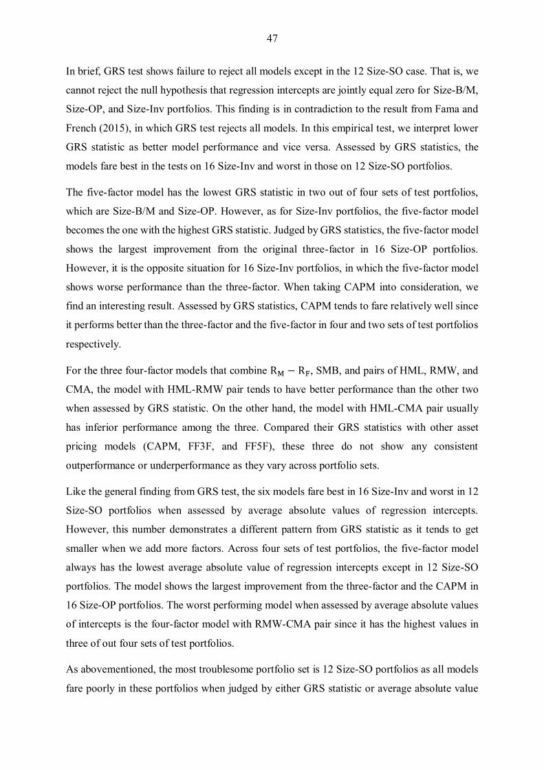
47

In brief, GRS test shows failure to reject all models except in the 12 Size-SO case. That is, we

cannot reject the null hypothesis that regression intercepts are jointly equal zero for Size-B/M,

Size-OP, and Size-Inv portfolios. This finding is in contradiction to the result from Fama and

French (2015), in which GRS test rejects all models. In this empirical test, we interpret lower

GRS statistic as better model performance and vice versa. Assessed by GRS statistics, the

models fare best in the tests on 16 Size-Inv and worst in those on 12 Size-SO portfolios.

The five-factor model has the lowest GRS statistic in two out of four sets of test portfolios,

which are Size-B/M and Size-OP. However, as for Size-Inv portfolios, the five-factor model

becomes the one with the highest GRS statistic. Judged by GRS statistics, the five-factor model

shows the largest improvement from the original three-factor in 16 Size-OP portfolios.

However, it is the opposite situation for 16 Size-Inv portfolios, in which the five-factor model

shows worse performance than the three-factor. When taking CAPM into consideration, we

find an interesting result. Assessed by GRS statistics, CAPM tends to fare relatively well since

it performs better than the three-factor and the five-factor in four and two sets of test portfolios

respectively.

For the three four-factor models that combine RM − RF, SMB, and pairs of HML, RMW, and

CMA, the model with HML-RMW pair tends to have better performance than the other two

when assessed by GRS statistic. On the other hand, the model with HML-CMA pair usually

has inferior performance among the three. Compared their GRS statistics with other asset

pricing models (CAPM, FF3F, and FF5F), these three do not show any consistent

outperformance or underperformance as they vary across portfolio sets.

Like the general finding from GRS test, the six models fare best in 16 Size-Inv and worst in 12

Size-SO portfolios when assessed by average absolute values of regression intercepts.

However, this number demonstrates a different pattern from GRS statistic as it tends to get

smaller when we add more factors. Across four sets of test portfolios, the five-factor model

always has the lowest average absolute value of regression intercepts except in 12 Size-SO

portfolios. The model shows the largest improvement from the three-factor and the CAPM in

16 Size-OP portfolios. The worst performing model when assessed by average absolute values

of intercepts is the four-factor model with RMW-CMA pair since it has the highest values in

three of out four sets of test portfolios.

As abovementioned, the most troublesome portfolio set is 12 Size-SO portfolios as all models

fare poorly in these portfolios when judged by either GRS statistic or average absolute value

48

of intercepts. For example, GRS test rejects all models except CAPM at 10% significance level.

The three-factor model and four-factor model with HML-CMA pair can even be rejected at 1%

significance level. Besides, the average absolute values of intercepts in this test portfolio set

are higher than those in other sets. This finding suggests that our six asset pricing models have

trouble explaining average returns of portfolios formed on size and state-ownership status.

Table 12 Average adjusted R2s for tests of six asset pricing models (CAPM and three-, four-, and five-factor

models) across four sets of test portfolios (Size-B/M, Size-OP, Size-Inv, and Size-SO); July 2009 -

December 2017, 102 months.

Size-B/M Size-OP Size-Inv Size-SO Average

CAPM 0.459 0.443 0.458 0.463 0.456

FF3F 0.727 0.689 0.683 0.692 0.698

FF5F 0.728 0.703 0.698 0.696 0.706

FF4F (HML-RMW) 0.727 0.704 0.685 0.696 0.703

FF4F (HML-CMA) 0.728 0.687 0.697 0.693 0.701

FF4F (RMW-CMA) 0.699 0.690 0.684 0.687 0.690

Table 12 presents average adjusted R2s for different models and portfolio sets. Across portfolio

sets, there seems to be no significant disparity in average adjusted R2 for different models.

Across models, the average adjusted R2 shows large improvement from CAPM to the three-

factor model (24.18% on average). However, there is minor improvement from the three-factor

to the five-factor model (0.88% on average). As for the three four-factor models, there is minor

enhancement or even deterioration (RMW-CMA pair) in average adjusted R2 from the three-

factor model. Compared with the five-factor model, these four-factor models have lower

average adjusted R2 but the difference is paltry. Much of these phenomena can be attributed to

relatively high correlation among HML, RMW, and CMA. For example, since there exists

extremely high correlation between HML and RMW (-0.79), replacing one factor with the

other does not significantly affect explanatory power of the model.

In brief, this analysis of average adjusted R2 only describes the aggregate level as it overlooks

variation within each group. In Section 5.4.2 – 5.4.5, we will discuss regression results in depth

for each type of model and test portfolio. However, these sections only present the results for

CAPM, the three-factor model, and the five-factor model since the empirical test focuses on

these three models. Moreover, because there are 60 VW test portfolios with six asset pricing

models in total, this will make displaying the results more manageable and concise.

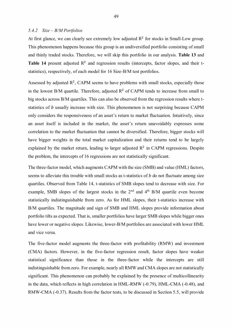
49

5.4.2 Size – B/M Portfolios

At first glance, we can clearly see extremely low adjusted R2 for stocks in Small-Low group.

This phenomenon happens because this group is an undiversified portfolio consisting of small

and thinly traded stocks. Therefore, we will skip this portfolio in our analysis. Table 13 and

Table 14 present adjusted R2 and regression results (intercepts, factor slopes, and their t-

statistics), respectively, of each model for 16 Size-B/M test portfolios.

Assessed by adjusted R2, CAPM seems to have problems with small stocks, especially those

in the lowest B/M quartile. Therefore, adjusted R2 of CAPM tends to increase from small to

big stocks across B/M quartiles. This can also be observed from the regression results where t-

statistics of 𝑏 usually increase with size. This phenomenon is not surprising because CAPM

only considers the responsiveness of an asset’s return to market fluctuation. Intuitively, since

an asset itself is included in the market, the asset’s return unavoidably expresses some

correlation to the market fluctuation that cannot be diversified. Therefore, bigger stocks will

have bigger weights in the total market capitalization and their returns tend to be largely

explained by the market return, leading to larger adjusted R2 in CAPM regressions. Despite

the problem, the intercepts of 16 regressions are not statistically significant.

The three-factor model, which augments CAPM with the size (SMB) and value (HML) factors,

seems to alleviate this trouble with small stocks as t-statistics of 𝑏 do not fluctuate among size

quartiles. Observed from Table 14, t-statistics of SMB slopes tend to decrease with size. For

example, SMB slopes of the largest stocks in the 2nd and 4th B/M quartile even become

statistically indistinguishable from zero. As for HML slopes, their t-statistics increase with

B/M quartiles. The magnitude and sign of SMB and HML slopes provide information about

portfolio tilts as expected. That is, smaller portfolios have larger SMB slopes while bigger ones

have lower or negative slopes. Likewise, lower-B/M portfolios are associated with lower HML

and vice versa.

The five-factor model augments the three-factor with profitability (RMW) and investment

(CMA) factors. However, in the five-factor regression result, factor slopes have weaker

statistical significance than those in the three-factor while the intercepts are still

indistinguishable from zero. For example, nearly all RMW and CMA slopes are not statistically

significant. This phenomenon can probably be explained by the presence of multicollinearity

in the data, which reflects in high correlation in HML-RMW (-0.79), HML-CMA (-0.48), and

RMW-CMA (-0.37). Results from the factor tests, to be discussed in Section 5.5, will provide

50

more evidence on this issue. Although RMW and CMA slopes are mainly indistinguishable

from zero, their magnitude and sign can still provide information about portfolio tilts. When

controlling for other factors, we find that these RMW and CMA slopes do not follow any

evident pattern across B/M quartiles, which does not line up with univariate characteristics

discussed in Section 5.1.6. However, there is no reason to expect multivariate regression slopes,

which estimate marginal effect holding other factors constant, will be consistent with univariate

characteristics (Fama and French, 2015).

51

Table 13 Adjusted R2 of CAPM, FF3F, and FF5F for 16 VW Size-B/M portfolios; July 2009 – December

2017, 102 months.

In June each year after rebalancing the sample, stocks are independently sorted into four size groups (Small

to Big) and four B/M groups (High to Low). The breakpoints are sample quartiles of size and B/M. The

intersection of these two sorts will generate 16 VW Size-B/M portfolios. Small-Low portfolio has extremely

low adjusted R2 across all three models because it is an undiversified portfolio consisting of small and thinly

traded stocks. Therefore, we will skip this portfolio in our analysis.

Panel A: CAPM

Low 2 3 High

Small 0.02 0.26 0.32 0.29

2 0.28 0.46 0.40 0.45

3 0.47 0.55 0.51 0.47

Big 0.74 0.66 0.63 0.41

Panel B: FF3F

Small 0.01 0.57 0.74 0.74

2 0.59 0.76 0.78 0.83

3 0.63 0.67 0.76 0.75

Big 0.79 0.76 0.75 0.76

Panel C: FF5F

Small -0.01 0.57 0.74 0.74

2 0.60 0.75 0.79 0.84

3 0.62 0.66 0.76 0.75

Big 0.80 0.79 0.76 0.76

52

Table 14 Regression results (intercepts, factor slopes, and their t-statistics) of CAPM, FF3F, and FF5F for

16 VW Size-B/M portfolios; July 2009 - December 2017, 102 months.


to Big) and four B/M groups (High to Low). The breakpoints are sample quartiles of size and B/M. The

intersection of these two sorts will generate 16 VW Size-B/M portfolios. Small-Low portfolio is an

undiversified portfolio consisting of small and thinly traded stocks and thus it will be excluded from our

analysis. Italic, Bold-Italic, and Bold font styles represent statistical significance at the 10%, 5%, and 1%

levels, respectively.

B/M Low 2 3 High Low 2 3 High

Panel A: CAPM

a t(a)

Small 0.008 0.004 0.008 0.006 0.72 0.67 1.21 0.90

2 -0.002 0.005 0.002 -0.003 -0.41 0.91 0.28 -0.53

3 -0.005 -0.004 -0.001 0.004 -0.93 -0.80 -0.31 0.64

Big 0.002 -0.003 -0.001 -0.002 0.82 -0.69 -0.24 -0.29

b t(b)

Small 0.34 0.76 0.86 0.78 1.68 6.02 7.02 6.43

2 0.72 1.02 0.93 1.04 6.39 9.37 8.34 9.10

3 0.95 0.98 0.94 1.13 9.48 11.14 10.26 9.43

Big 0.96 1.08 1.32 1.21 16.99 13.90 13.15 8.38

Panel B: FF3F

a t(a)

Small 0.007 0.002 0.006 0.004 0.67 0.42 1.46 1.04

2 -0.005 0.003 0.000 -0.005 -1.05 0.83 -0.05 -1.41

3 -0.006 -0.004 -0.002 0.004 -1.41 -1.15 -0.71 0.84

Big 0.003 -0.002 0.000 -0.001 1.11 -0.69 -0.11 -0.31

b t(b)

Small 0.38 0.90 0.89 0.75 1.71 8.69 10.89 9.59

2 0.94 1.10 0.95 0.98 10.17 13.94 12.98 14.40

3 0.99 0.98 0.88 0.96 10.89 11.99 12.78 10.80

Big 0.94 0.92 1.10 0.86 17.07 13.29 12.42 8.64

s t(s)

Small 0.23 1.00 0.92 0.79 0.83 7.94 9.23 8.30

2 0.98 0.89 0.83 0.68 8.74 9.23 9.32 8.24

3 0.58 0.41 0.44 0.26 5.21 4.08 5.19 2.43

Big -0.25 -0.15 -0.29 -0.20 -3.65 -1.82 -2.71 -1.68

h t(h)

Small -0.01 0.09 0.48 0.61 -0.02 0.80 5.51 7.24

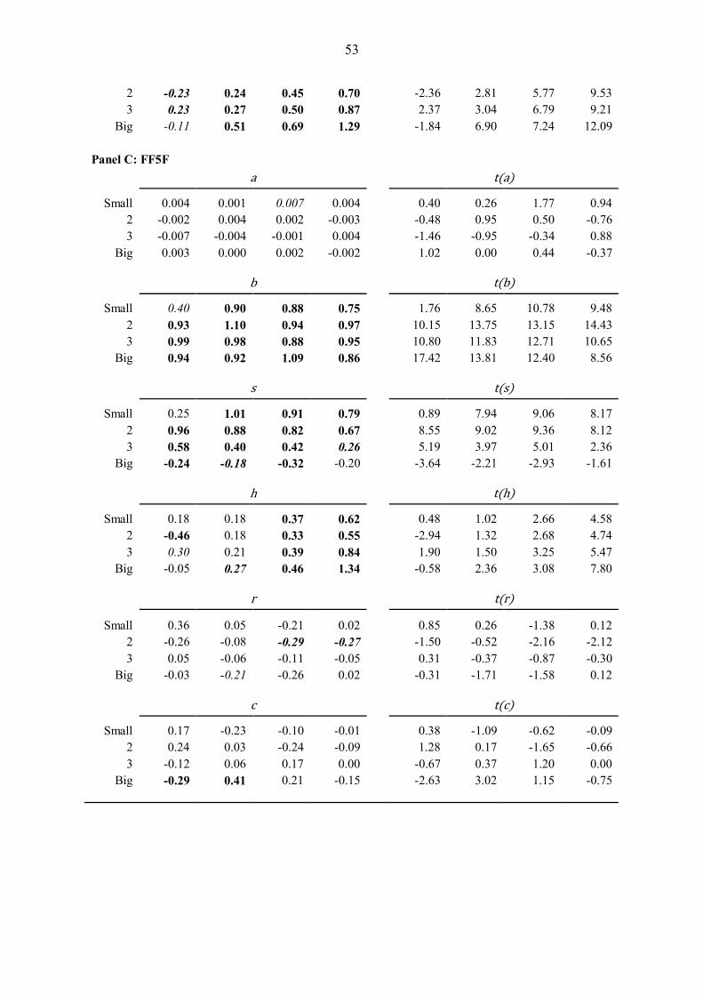
53

2 -0.23 0.24 0.45 0.70 -2.36 2.81 5.77 9.53

3 0.23 0.27 0.50 0.87 2.37 3.04 6.79 9.21

Big -0.11 0.51 0.69 1.29 -1.84 6.90 7.24 12.09

Panel C: FF5F

a t(a)

Small 0.004 0.001 0.007 0.004 0.40 0.26 1.77 0.94

2 -0.002 0.004 0.002 -0.003 -0.48 0.95 0.50 -0.76

3 -0.007 -0.004 -0.001 0.004 -1.46 -0.95 -0.34 0.88

Big 0.003 0.000 0.002 -0.002 1.02 0.00 0.44 -0.37

b t(b)

Small 0.40 0.90 0.88 0.75 1.76 8.65 10.78 9.48

2 0.93 1.10 0.94 0.97 10.15 13.75 13.15 14.43

3 0.99 0.98 0.88 0.95 10.80 11.83 12.71 10.65

Big 0.94 0.92 1.09 0.86 17.42 13.81 12.40 8.56

s t(s)

Small 0.25 1.01 0.91 0.79 0.89 7.94 9.06 8.17

2 0.96 0.88 0.82 0.67 8.55 9.02 9.36 8.12

3 0.58 0.40 0.42 0.26 5.19 3.97 5.01 2.36

Big -0.24 -0.18 -0.32 -0.20 -3.64 -2.21 -2.93 -1.61

h t(h)

Small 0.18 0.18 0.37 0.62 0.48 1.02 2.66 4.58

2 -0.46 0.18 0.33 0.55 -2.94 1.32 2.68 4.74

3 0.30 0.21 0.39 0.84 1.90 1.50 3.25 5.47

Big -0.05 0.27 0.46 1.34 -0.58 2.36 3.08 7.80

r t(r)

Small 0.36 0.05 -0.21 0.02 0.85 0.26 -1.38 0.12

2 -0.26 -0.08 -0.29 -0.27 -1.50 -0.52 -2.16 -2.12

3 0.05 -0.06 -0.11 -0.05 0.31 -0.37 -0.87 -0.30

Big -0.03 -0.21 -0.26 0.02 -0.31 -1.71 -1.58 0.12

c t(c)

Small 0.17 -0.23 -0.10 -0.01 0.38 -1.09 -0.62 -0.09

2 0.24 0.03 -0.24 -0.09 1.28 0.17 -1.65 -0.66

3 -0.12 0.06 0.17 0.00 -0.67 0.37 1.20 0.00

Big -0.29 0.41 0.21 -0.15 -2.63 3.02 1.15 -0.75

54

5.4.3 Size – OP Portfolios

Table 15 and Table 16 present adjusted R2s and regression results (intercepts, factor slopes,

and their t-statistics), respectively, of each model for 16 Size-OP test portfolios. Similar to

Size-B/M portfolios, adjusted R2 of CAPM tends to increase from small to big stocks across

OP quartiles. As adjusted R2 of CAPM is relatively high for big stocks, the three-factor model

shows lower improvement from CAPM for big stocks than for smaller ones. This phenomenon

is also reflected in the negative relation between t-statistics of SMB slopes and size, which is

similar to Size-B/M case.

The intercepts of 16 CAPM regressions are not statistically significant except for the largest

stocks in weak OP quartile. Although the three-factor model mitigates the problem with small

stocks, the trouble with big stocks in weak OP quartile remains and is resolved only when

profitability and investment factors are added. Implied from RMW and CMA slopes, this

portfolio is dominated by big stocks whose returns behave like those of unprofitable firms that

invest aggressively. It is intuitive that the three-factor model falls short on portfolios formed

from size and profitability, which is not included in the model. However, apart from this

troublesome portfolio of big stocks with weak profitability, the five-factor model shows minor

improvement or even deterioration in adjusted R2 from the three-factor as more than half of

RMW and all of CMA slopes are not statistically significant. Like other Size-B/M portfolios,

multivariate regression slopes tend not to line up with univariate characteristics since there is

no clear pattern in RMW and CMA across size and OP quartiles.

55

Table 15 Adjusted R2 of CAPM, FF3F, and FF5F for 16 VW Size-OP portfolios; July 2009 - December

2017, 102 months.


to Big) and four OP groups (Weak to Robust). The breakpoints are sample quartiles of size and OP. The

intersection of these two sorts will generate 16 VW Size-OP portfolios.

Panel A: CAPM

Weak 2 3 Robust

Small 0.24 0.22 0.32 0.28

2 0.43 0.43 0.38 0.46

3 0.38 0.56 0.47 0.52

Big 0.54 0.63 0.59 0.63

Panel B: FF3F

Small 0.67 0.64 0.70 0.47

2 0.80 0.78 0.76 0.76

3 0.70 0.74 0.62 0.67

Big 0.71 0.69 0.60 0.72

Panel C: FF5F

Small 0.68 0.64 0.69 0.51

2 0.83 0.79 0.76 0.76

3 0.72 0.74 0.61 0.66

Big 0.82 0.70 0.59 0.74

56


16 VW Size-OP portfolios; July 2009 - December 2017, 102 months.


to Big) and four OP groups (Weak to Robust). The breakpoints are sample quartiles of size and OP. The

intersection of these two sorts will generate 16 VW Size-OP portfolios. Italic, Bold-Italic, and Bold font

styles represent statistical significance at the 10%, 5%, and 1% levels, respectively.

OP Weak 2 3 Robust Weak 2 3 Robust

Panel A: CAPM

a t(a)

Small 0.008 0.002 0.002 0.010 0.87 0.37 0.31 1.67

2 -0.003 -0.002 0.004 0.003 -0.44 -0.32 0.82 0.62

3 -0.003 -0.003 -0.002 -0.002 -0.46 -0.65 -0.49 -0.33

Big -0.010 -0.001 -0.002 0.004 -2.01 -0.31 -0.48 1.10

b t(b)

Small 0.97 0.72 0.73 0.76 5.76 5.51 6.92 6.33

2 1.06 1.01 0.83 0.92 8.86 8.84 7.91 9.25

3 1.08 1.03 0.90 0.99 7.93 11.28 9.48 10.50

Big 1.12 1.21 0.97 0.88 11.04 13.10 12.14 13.25

Panel B: FF3F

a t(a)

Small 0.005 0.000 0.000 0.009 0.95 0.08 -0.10 1.65

2 -0.004 -0.004 0.002 0.001 -1.14 -0.99 0.66 0.40

3 -0.004 -0.004 -0.003 -0.003 -0.82 -1.04 -0.80 -0.69

Big -0.010 -0.001 -0.002 0.004 -2.46 -0.22 -0.38 1.47

b t(b)

Small 0.93 0.77 0.83 0.83 7.69 8.06 11.01 7.46

2 1.00 1.02 0.97 0.99 13.06 13.27 13.69 13.98

3 0.92 0.96 0.90 1.03 8.91 12.70 10.26 12.10

Big 0.93 1.07 0.91 0.88 10.66 11.61 10.57 14.19

s t(s)

Small 1.01 0.97 0.91 0.71 6.87 8.29 9.85 5.20

2 0.70 0.82 1.00 0.82 7.53 8.75 11.51 9.42

3 0.41 0.34 0.44 0.55 3.24 3.64 4.14 5.35

Big -0.07 -0.19 -0.18 -0.28 -0.66 -1.69 -1.69 -3.72

h t(h)

Small 0.83 0.40 0.16 0.17 6.46 3.91 2.02 1.41

2 0.68 0.47 0.09 0.24 8.31 5.68 1.21 3.18

3 0.91 0.50 0.30 0.20 8.21 6.14 3.22 2.16

Big 0.70 0.44 0.14 -0.21 7.52 4.48 1.55 -3.10

57

Panel C: FF5F

a t(a)

Small 0.008 0.002 -0.002 0.004 1.35 0.40 -0.40 0.74

2 0.001 -0.001 0.002 0.000 0.23 -0.27 0.54 -0.04

3 0.001 -0.004 -0.004 -0.004 0.17 -0.92 -0.82 -1.04

Big -0.002 0.002 -0.002 0.002 -0.70 0.49 -0.52 0.59

b t(b)

Small 0.91 0.77 0.84 0.86 7.65 7.95 11.03 7.94

2 0.98 1.01 0.97 1.00 13.97 13.31 13.57 14.03

3 0.90 0.96 0.90 1.03 9.09 12.54 10.15 12.13

Big 0.89 1.05 0.91 0.89 13.04 11.75 10.49 14.75

s t(s)

Small 0.99 0.96 0.92 0.75 6.80 8.13 9.84 5.66

2 0.66 0.80 1.00 0.83 7.70 8.61 11.41 9.53

3 0.36 0.34 0.45 0.57 2.99 3.58 4.10 5.44

Big -0.13 -0.21 -0.17 -0.26 -1.61 -1.95 -1.61 -3.50

h t(h)

Small 0.67 0.29 0.25 0.54 3.28 1.77 1.90 2.91

2 0.28 0.26 0.14 0.38 2.30 2.00 1.10 3.10

3 0.47 0.50 0.33 0.33 2.78 3.78 2.19 2.29

Big 0.09 0.22 0.20 0.01 0.81 1.41 1.37 0.09

r t(r)

Small -0.38 -0.22 0.15 0.61 -1.72 -1.23 1.07 3.03

2 -0.61 -0.33 0.01 0.17 -4.67 -2.32 0.09 1.25

3 -0.55 -0.04 0.03 0.20 -2.95 -0.29 0.18 1.25

Big -1.00 -0.43 0.08 0.31 -7.86 -2.57 0.49 2.77

c t(c)

Small -0.32 -0.13 0.06 0.11 -1.33 -0.66 0.36 0.49

2 0.03 -0.02 -0.13 -0.11 0.23 -0.15 -0.92 -0.76

3 0.31 -0.09 -0.04 -0.03 1.56 -0.61 -0.23 -0.19

Big -0.18 -0.21 -0.04 -0.04 -1.27 -1.14 -0.20 -0.34

58

5.4.4 Size – Inv Portfolios

Table 17 and Table 18 present adjusted R2s and regression results (intercepts, factor slopes,

and their t-statistics), respectively, of each model for 16 Size-Inv test portfolios. In general, the

multivariate regression results for Size-Inv portfolios are somewhat similar to the previous two

cases. To begin with, adjusted R2 of CAPM also increases from small to big stocks across Inv

quartiles and the three-factor model shows lower improvement from CAPM for big stocks than

for smaller ones. Furthermore, the five-factor model shows minor improvement or even

deterioration in adjusted R2 from the three-factor as the majority of RMW and CMA slopes are

not statistically significant. Finally, multivariate regression slopes do not line up with

univariate characteristics since there is no clear pattern in HML and RMW slopes across size

and Inv quartiles.

59

Table 17 Adjusted R2 of CAPM, FF3F, and FF5F for 16 VW Size-Inv portfolios; July 2009 - December 2017,

102 months.

In June each year after rebalancing the sample, stocks are independently sorted into four size groups, Small

to Big, and four Inv groups, Conservative (Cons.) to Aggressive (Aggr.). The breakpoints are sample

quartiles of size and Inv. The intersection of these two sorts will generate 16 VW Size-Inv portfolios.

Panel A: CAPM

Cons. 2 3 Aggr.

Small 0.30 0.21 0.20 0.41

2 0.49 0.38 0.40 0.42

3 0.46 0.52 0.50 0.53

Big 0.60 0.64 0.69 0.56

Panel B: FF3F

Small 0.69 0.56 0.54 0.70

2 0.83 0.77 0.71 0.71

3 0.66 0.73 0.71 0.66

Big 0.69 0.68 0.69 0.59

Panel C: FF5F

Small 0.71 0.55 0.55 0.73

2 0.83 0.78 0.71 0.73

3 0.66 0.73 0.71 0.65

Big 0.74 0.68 0.70 0.71

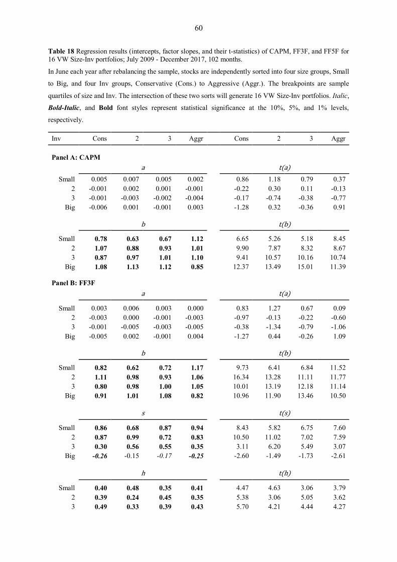
60


16 VW Size-Inv portfolios; July 2009 - December 2017, 102 months.

In June each year after rebalancing the sample, stocks are independently sorted into four size groups, Small

to Big, and four Inv groups, Conservative (Cons.) to Aggressive (Aggr.). The breakpoints are sample

quartiles of size and Inv. The intersection of these two sorts will generate 16 VW Size-Inv portfolios. Italic,

Bold-Italic, and Bold font styles represent statistical significance at the 10%, 5%, and 1% levels,

respectively.

Inv Cons 2 3 Aggr Cons 2 3 Aggr

Panel A: CAPM

a t(a)

Small 0.005 0.007 0.005 0.002 0.86 1.18 0.79 0.37

2 -0.001 0.002 0.001 -0.001 -0.22 0.30 0.11 -0.13

3 -0.001 -0.003 -0.002 -0.004 -0.17 -0.74 -0.38 -0.77

Big -0.006 0.001 -0.001 0.003 -1.28 0.32 -0.36 0.91

b t(b)

Small 0.78 0.63 0.67 1.12 6.65 5.26 5.18 8.45

2 1.07 0.88 0.93 1.01 9.90 7.87 8.32 8.67

3 0.87 0.97 1.01 1.10 9.41 10.57 10.16 10.74

Big 1.08 1.13 1.12 0.85 12.37 13.49 15.01 11.39

Panel B: FF3F

a t(a)

Small 0.003 0.006 0.003 0.000 0.83 1.27 0.67 0.09

2 -0.003 0.000 -0.001 -0.003 -0.97 -0.13 -0.22 -0.60

3 -0.001 -0.005 -0.003 -0.005 -0.38 -1.34 -0.79 -1.06

Big -0.005 0.002 -0.001 0.004 -1.27 0.44 -0.26 1.09

b t(b)

Small 0.82 0.62 0.72 1.17 9.73 6.41 6.84 11.52

2 1.11 0.98 0.93 1.06 16.34 13.28 11.11 11.77

3 0.80 0.98 1.00 1.05 10.01 13.19 12.18 11.14

Big 0.91 1.01 1.08 0.82 10.96 11.90 13.46 10.50

s t(s)

Small 0.86 0.68 0.87 0.94 8.43 5.82 6.75 7.60

2 0.87 0.99 0.72 0.83 10.50 11.02 7.02 7.59

3 0.30 0.56 0.55 0.35 3.11 6.20 5.49 3.07

Big -0.26 -0.15 -0.17 -0.25 -2.60 -1.49 -1.73 -2.61

h t(h)

Small 0.40 0.48 0.35 0.41 4.47 4.63 3.06 3.79

2 0.39 0.24 0.45 0.35 5.38 3.06 5.05 3.62

3 0.49 0.33 0.39 0.43 5.70 4.21 4.44 4.27

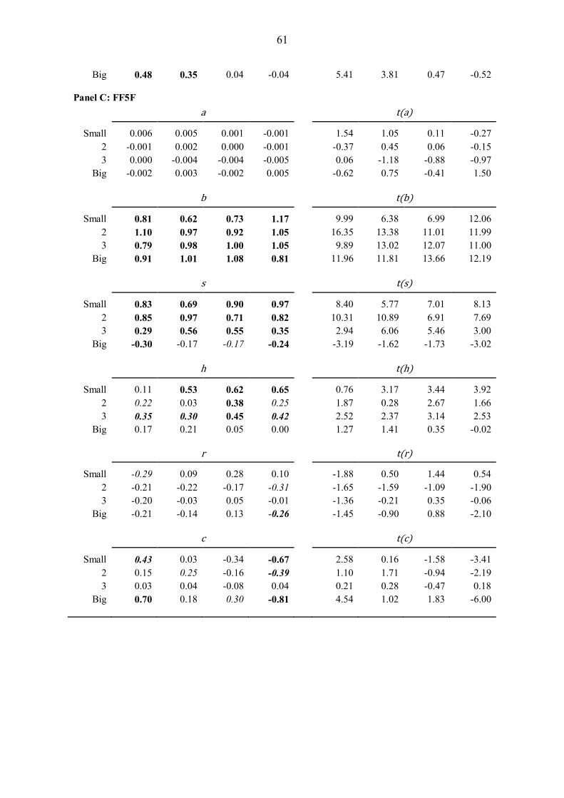
61

Big 0.48 0.35 0.04 -0.04 5.41 3.81 0.47 -0.52

Panel C: FF5F

a t(a)

Small 0.006 0.005 0.001 -0.001 1.54 1.05 0.11 -0.27

2 -0.001 0.002 0.000 -0.001 -0.37 0.45 0.06 -0.15

3 0.000 -0.004 -0.004 -0.005 0.06 -1.18 -0.88 -0.97

Big -0.002 0.003 -0.002 0.005 -0.62 0.75 -0.41 1.50

b t(b)

Small 0.81 0.62 0.73 1.17 9.99 6.38 6.99 12.06

2 1.10 0.97 0.92 1.05 16.35 13.38 11.01 11.99

3 0.79 0.98 1.00 1.05 9.89 13.02 12.07 11.00

Big 0.91 1.01 1.08 0.81 11.96 11.81 13.66 12.19

s t(s)

Small 0.83 0.69 0.90 0.97 8.40 5.77 7.01 8.13

2 0.85 0.97 0.71 0.82 10.31 10.89 6.91 7.69

3 0.29 0.56 0.55 0.35 2.94 6.06 5.46 3.00

Big -0.30 -0.17 -0.17 -0.24 -3.19 -1.62 -1.73 -3.02

h t(h)

Small 0.11 0.53 0.62 0.65 0.76 3.17 3.44 3.92

2 0.22 0.03 0.38 0.25 1.87 0.28 2.67 1.66

3 0.35 0.30 0.45 0.42 2.52 2.37 3.14 2.53

Big 0.17 0.21 0.05 0.00 1.27 1.41 0.35 -0.02

r t(r)

Small -0.29 0.09 0.28 0.10 -1.88 0.50 1.44 0.54

2 -0.21 -0.22 -0.17 -0.31 -1.65 -1.59 -1.09 -1.90

3 -0.20 -0.03 0.05 -0.01 -1.36 -0.21 0.35 -0.06

Big -0.21 -0.14 0.13 -0.26 -1.45 -0.90 0.88 -2.10

c t(c)

Small 0.43 0.03 -0.34 -0.67 2.58 0.16 -1.58 -3.41

2 0.15 0.25 -0.16 -0.39 1.10 1.71 -0.94 -2.19

3 0.03 0.04 -0.08 0.04 0.21 0.28 -0.47 0.18

Big 0.70 0.18 0.30 -0.81 4.54 1.02 1.83 -6.00

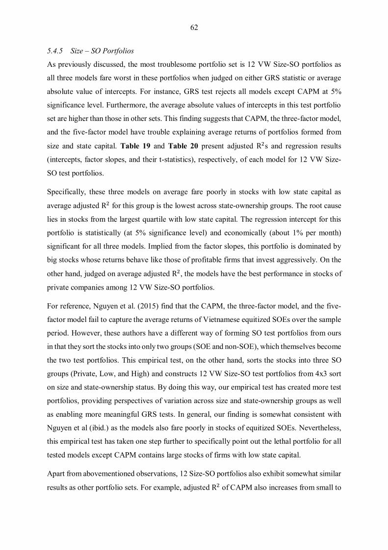
62

5.4.5 Size – SO Portfolios

As previously discussed, the most troublesome portfolio set is 12 VW Size-SO portfolios as

all three models fare worst in these portfolios when judged on either GRS statistic or average

absolute value of intercepts. For instance, GRS test rejects all models except CAPM at 5%

significance level. Furthermore, the average absolute values of intercepts in this test portfolio

set are higher than those in other sets. This finding suggests that CAPM, the three-factor model,

and the five-factor model have trouble explaining average returns of portfolios formed from

size and state capital. Table 19 and Table 20 present adjusted R2s and regression results

(intercepts, factor slopes, and their t-statistics), respectively, of each model for 12 VW Size-

SO test portfolios.

Specifically, these three models on average fare poorly in stocks with low state capital as

average adjusted R2 for this group is the lowest across state-ownership groups. The root cause

lies in stocks from the largest quartile with low state capital. The regression intercept for this

portfolio is statistically (at 5% significance level) and economically (about 1% per month)

significant for all three models. Implied from the factor slopes, this portfolio is dominated by

big stocks whose returns behave like those of profitable firms that invest aggressively. On the

other hand, judged on average adjusted R2, the models have the best performance in stocks of

private companies among 12 VW Size-SO portfolios.

For reference, Nguyen et al. (2015) find that the CAPM, the three-factor model, and the five-

factor model fail to capture the average returns of Vietnamese equitized SOEs over the sample

period. However, these authors have a different way of forming SO test portfolios from ours

in that they sort the stocks into only two groups (SOE and non-SOE), which themselves become

the two test portfolios. This empirical test, on the other hand, sorts the stocks into three SO

groups (Private, Low, and High) and constructs 12 VW Size-SO test portfolios from 4x3 sort

on size and state-ownership status. By doing this way, our empirical test has created more test

portfolios, providing perspectives of variation across size and state-ownership groups as well

as enabling more meaningful GRS tests. In general, our finding is somewhat consistent with

Nguyen et al (ibid.) as the models also fare poorly in stocks of equitized SOEs. Nevertheless,

this empirical test has taken one step further to specifically point out the lethal portfolio for all

tested models except CAPM contains large stocks of firms with low state capital.

Apart from abovementioned observations, 12 Size-SO portfolios also exhibit somewhat similar

results as other portfolio sets. For example, adjusted R2 of CAPM also increases from small to

63

big stocks and the three-factor model shows larger improvement from CAPM for smaller

stocks than for bigger ones. Moreover, the five-factor model shows minor improvement or

even deterioration in adjusted R2 from the three-factor as RMW and CMA slopes are mostly

not statistically indistinguishable from zero. Finally, multivariate regression slopes do not line

up with univariate characteristics since there is no clear pattern in HML, RMW, and CMA

slopes across size and state-ownership groups.

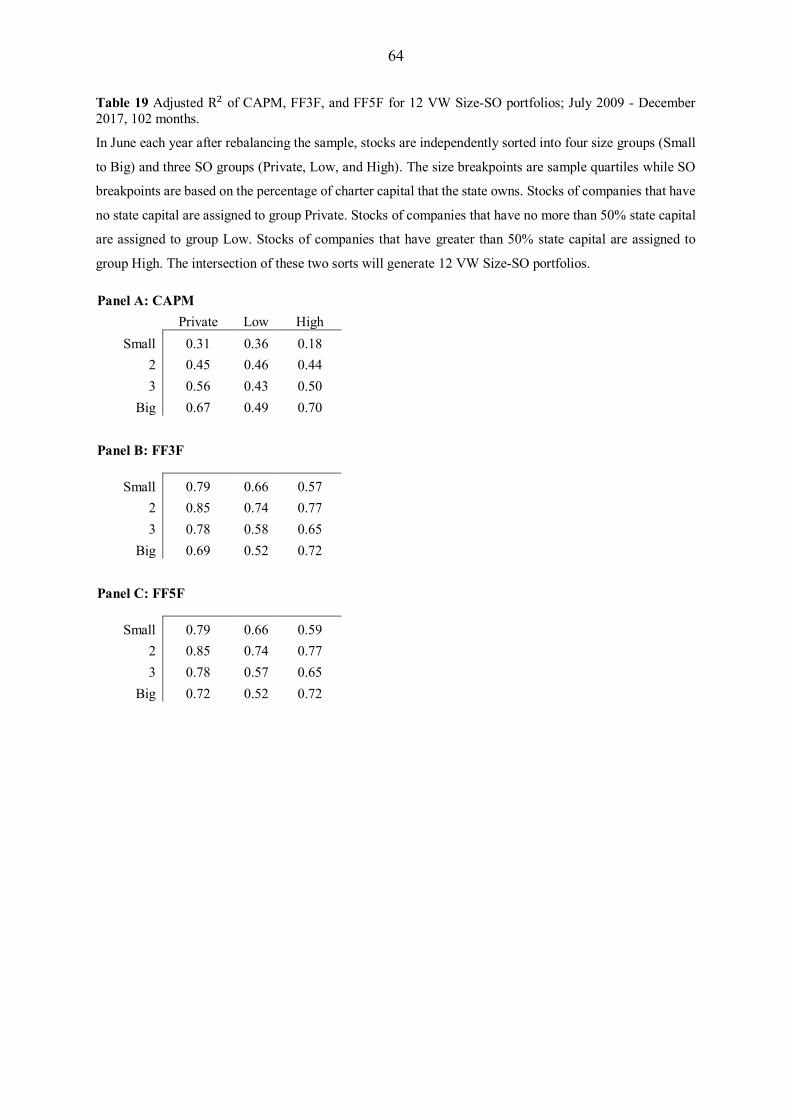
64

Table 19 Adjusted R2 of CAPM, FF3F, and FF5F for 12 VW Size-SO portfolios; July 2009 - December

2017, 102 months.


to Big) and three SO groups (Private, Low, and High). The size breakpoints are sample quartiles while SO

breakpoints are based on the percentage of charter capital that the state owns. Stocks of companies that have

no state capital are assigned to group Private. Stocks of companies that have no more than 50% state capital

are assigned to group Low. Stocks of companies that have greater than 50% state capital are assigned to

group High. The intersection of these two sorts will generate 12 VW Size-SO portfolios.

Panel A: CAPM

Private Low High

Small 0.31 0.36 0.18

2 0.45 0.46 0.44

3 0.56 0.43 0.50

Big 0.67 0.49 0.70

Panel B: FF3F

Small 0.79 0.66 0.57

2 0.85 0.74 0.77

3 0.78 0.58 0.65

Big 0.69 0.52 0.72

Panel C: FF5F

Small 0.79 0.66 0.59

2 0.85 0.74 0.77

3 0.78 0.57 0.65

Big 0.72 0.52 0.72

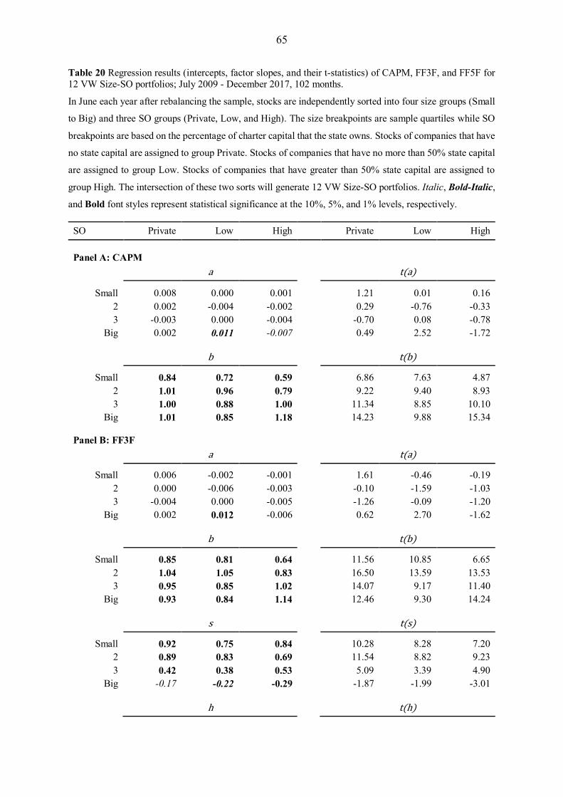
65


12 VW Size-SO portfolios; July 2009 - December 2017, 102 months.


to Big) and three SO groups (Private, Low, and High). The size breakpoints are sample quartiles while SO

breakpoints are based on the percentage of charter capital that the state owns. Stocks of companies that have

no state capital are assigned to group Private. Stocks of companies that have no more than 50% state capital

are assigned to group Low. Stocks of companies that have greater than 50% state capital are assigned to

group High. The intersection of these two sorts will generate 12 VW Size-SO portfolios. Italic, Bold-Italic,

and Bold font styles represent statistical significance at the 10%, 5%, and 1% levels, respectively.

SO Private Low High Private Low High

Panel A: CAPM

a t(a)

Small 0.008 0.000 0.001 1.21 0.01 0.16

2 0.002 -0.004 -0.002 0.29 -0.76 -0.33

3 -0.003 0.000 -0.004 -0.70 0.08 -0.78

Big 0.002 0.011 -0.007 0.49 2.52 -1.72

b t(b)

Small 0.84 0.72 0.59 6.86 7.63 4.87

2 1.01 0.96 0.79 9.22 9.40 8.93

3 1.00 0.88 1.00 11.34 8.85 10.10

Big 1.01 0.85 1.18 14.23 9.88 15.34

Panel B: FF3F

a t(a)

Small 0.006 -0.002 -0.001 1.61 -0.46 -0.19

2 0.000 -0.006 -0.003 -0.10 -1.59 -1.03

3 -0.004 0.000 -0.005 -1.26 -0.09 -1.20

Big 0.002 0.012 -0.006 0.62 2.70 -1.62

b t(b)

Small 0.85 0.81 0.64 11.56 10.85 6.65

2 1.04 1.05 0.83 16.50 13.59 13.53

3 0.95 0.85 1.02 14.07 9.17 11.40

Big 0.93 0.84 1.14 12.46 9.30 14.24

s t(s)

Small 0.92 0.75 0.84 10.28 8.28 7.20

2 0.89 0.83 0.69 11.54 8.82 9.23

3 0.42 0.38 0.53 5.09 3.39 4.90

Big -0.17 -0.22 -0.29 -1.87 -1.99 -3.01

h t(h)

66

Small 0.56 0.15 0.37 7.08 1.82 3.58

2 0.45 0.19 0.28 6.71 2.28 4.30

3 0.48 0.35 0.27 6.64 3.52 2.87

Big 0.21 -0.11 -0.02 2.68 -1.18 -0.24

Panel C: FF5F

a t(a)

Small 0.005 -0.001 0.003 1.27 -0.26 0.58

2 0.002 -0.004 -0.002 0.56 -1.11 -0.71

3 -0.004 0.001 -0.005 -1.03 0.12 -1.14

Big 0.004 0.009 -0.006 1.16 2.02 -1.44

b t(b)

Small 0.85 0.81 0.62 11.57 10.82 6.61

2 1.03 1.05 0.82 16.62 13.46 13.38

3 0.95 0.84 1.02 13.93 9.04 11.27

Big 0.92 0.85 1.14 12.96 9.47 14.11

s t(s)

Small 0.93 0.74 0.81 10.35 8.13 7.02

2 0.87 0.82 0.68 11.47 8.63 9.06

3 0.41 0.38 0.53 4.95 3.29 4.84

Big -0.18 -0.20 -0.30 -2.09 -1.79 -3.02

h t(h)

Small 0.67 0.06 0.07 5.28 0.49 0.40

2 0.30 0.07 0.23 2.81 0.52 2.14

3 0.42 0.28 0.29 3.62 1.77 1.89

Big 0.12 0.10 -0.07 0.98 0.66 -0.49

r t(r)

Small 0.09 -0.04 -0.43 0.63 -0.31 -2.45

2 -0.27 -0.20 -0.12 -2.33 -1.38 -1.02

3 -0.05 -0.14 -0.02 -0.36 -0.80 -0.14

Big -0.31 0.30 -0.02 -2.32 1.80 -0.15

c t(c)

Small -0.20 0.21 0.08 -1.34 1.39 0.44

2 -0.08 -0.04 -0.08 -0.63 -0.25 -0.62

3 0.11 -0.09 -0.13 0.76 -0.50 -0.70

Big -0.40 -0.07 0.13 -2.79 -0.38 0.77

67

5.5 Factor Spanning Test Results

Table 21 shows the results from regressing each of the five factor return on the other four. As

expected from the highly negative correlation coefficient, both HML and RMW slopes in

RMW and HML regression respectively are negative and statistically significant (t-stat = -

10.16). These two factor regressions also show relatively high adjusted R2. Besides RMW,

average HML return is also captured by CMA as CMA slope in HML regression is statistically

different from zero. However, the intercept from HML regression is still statistically (t-stat =

2.24) and economically (1% a month) significant, similar to the intercept from RMW

regression. On the other hand, average CMA return is fully captured by its exposure to other

factors, especially HML (t-stat = 3.42), since CMA regression intercept is indistinguishable

from zero.

As for the market excess return and SMB regressions, their adjusted R2s are relatively low,

approximately 12%. Nevertheless, the intercepts from both regressions are not statistically

different from zero. SMB slope in market excess return regression is statistically significant as

market excess return slope in SMB regression, both with t-stat around 0.88-0.89.

Table 21 Factor Test Results

Using four factors in regressions to explain average returns on the fifth: July 2009 - December 2017, 102

months.




(conservative-minus-aggressive) is the investment factor. All the factors are constructed from independent

sorts of stocks into two Size groups and three B/M groups, three OP groups, or three Inv groups.

Int 𝐑𝐌 − 𝐑𝐅 SMB HML RMW CMA 𝐀𝐝𝐣. 𝐑𝟐

𝐑𝐌 − 𝐑𝐅

Coefficient 0.004 -0.36 0.28 -0.13 -0.02 0.12

t-Statistic 0.88 -2.99 1.61 -0.67 -0.07

SMB

Coefficient 0.004 -0.24 0.16 -0.16 0.08 0.12

t-Statistic 0.89 -2.99 1.10 -1.06 0.46

HML

Coefficient 0.01 0.09 0.08 -0.78 0.39 0.66

t-Statistic 2.24 1.61 1.10 -10.16 3.42

68

RMW

Coefficient 0.01 -0.04 -0.07 -0.66 0.03 0.61

t-Statistic 3.12 -0.67 -1.06 -10.16 0.25

CMA

Coefficient 0.002 0.00 0.03 0.28 0.02 0.20

t-Statistic -0.66 -0.07 0.46 3.42 0.25

In the spirit of Huberman and Kandel (1987), the factor spanning tests suggest that adding

HML will improve the mean-variance-efficient tangency portfolio by combining the risk-free

asset, the market portfolio, SMB, RMW, and CMA. That is, HML is not a redundant factor as

Fama and French (2015) find in US data for 1963–2013. This finding is consistent with that

from Nguyen et al. (2015) and many other empirical tests in different markets discussed in

Section 2.5.3. In this empirical test, adding HML to a two-factor model that includes market

excess return and SMB will improve the average adjusted R2 by approximately 7%.

If a factor must be chosen as the redundant one, CMA appears to be the most promising

candidate. Firstly, the intercept from CMA regression is not distinguishable from zero as

average CMA return is fully absorbed by its exposure to other factors, especially HML.

Secondly, the majority of CMA slopes in the five-factor regressions are not statistically

significant. Thirdly, the five-factor model shows minuscule improvement or even deterioration

in the description of average returns (assessed by average adjusted R2) from the five-factor

model that drops CMA (Table 12). The redundancy of CMA is similar to the findings of Guo

et al. (2017) in Chinese market during 1995 -2014 and those of Fama and French (2017) in

Europe, Japan, and Asia Pacific during 1990 -2015.

Another potential candidate is RMW. Although the intercept from RMW regression is

statistically significant at 1% significance level, average RMW return is largely explained by

its exposure to HML, mainly due to the highly negative correlation between these two factors

of –0.79. When not simultaneously included in a model, HML and RMW do equally well in

enhancing the description of average returns. Specifically, a three-factor model that replaces

HML with RMW produces almost the same average adjusted R2 of approximately 69.4%.

However, when both HML and RMW are incorporated, the majority of HML slopes are

statistically significant while most RMW slopes are not. Furthermore, the five-factor model

69

also exhibits paltry improvement (assessed by average adjusted R2) from the five-factor model

that drops RMW.

The remaining two factors, market excess return and SMB, do a plausible job in improving the

description of average returns. Excess market return on its own captures 45.6% of variation in

stock returns on average and SMB improves this statistic by 17.2% to 62.8% when

incorporated. In brief, the findings from both asset pricing tests and factor spanning tests

suggest that the value factor, HML, does not become redundant when profitability, RMW, and

investment, CMA, factors are added into the model. Instead, RMW and CMA factor returns

are largely absorbed by their exposure to HML. However, it is important to note that factor

spanning inferences should be taken with caution since they tend to be sample specific (Fama

and French, 2017).

70

6 CONCLUSION

6.1 Main Findings

There are weak patterns in average returns related to Size, B/M, profitability, investment, and

state ownership in that they are not smooth or not evident. Likewise, other than RMW, all FF

factors constructed in this empirical test demonstrate weaker or even reverse behavior

compared to what Fama and French (2015) expect. For example, we document negative

cumulative return of CMA throughout the test period from June 2009 to December 2017, which

means stocks of companies that invest aggressively tend to outperform those with conservative

investment level. Table 22 summarizes the expectation and empirical results of the patterns in

average returns.

Table 22 Patterns in Average Returns: Expectation and Empirical Result

Pattern in average

returns

Expectation Empirical Result

Size effect

Average return

decreases with Size

Average returns do not usually decrease with

size. However, smallest stocks almost always

earn the highest average returns.

Value effect Average return

increases with B/M

No clear pattern

Profitability effect Average return

increases with OP

Weak OP tends to have lower average returns than

Robust OP. However, the effect is not smooth

Investment effect Average return

decreases with Inv

No clear pattern. Reversal happens in some instances

State-ownership

effect

For small stocks (1st & 2nd size quartile), stocks of

private companies earn the highest average returns

For big stocks (3rd & 4th size quartile), stocks of

low-state-capital companies earn the highest

average returns

Stocks of high-state-capital companies have

relatively low average return across all size

quartiles.

71

Regarding asset pricing tests, the GRS test fails to reject all models except in 12 VW Size-SO

portfolios. This finding is in contradiction to the result from Fama and French (2015) but

consistent with that from Nguyen et al. (2015). Judged on either GRS statistics or average

absolute values of intercepts, all models fare worst in these 12 VW Size-SO portfolios,

suggesting that our asset pricing models have trouble explaining average returns of portfolios

formed from size and state-ownership status. Indeed, we can conclude that the lethal portfolio

for all tested models except CAPM contains large stocks of firms with low state capital (more

than 0 and less than 50% of charter capital). Particularly, the regression intercept for this

portfolio is statistically (at 5% significance level) and economically (about 1% per month)

significant for all three models. The average adjusted R2s of the CAPM, the three-factor model,

and the five-factor model are respectively 45.6%, 69.8%, and 70.6%.

Regarding factor redundancy issue, HML is not a redundant factor in this empirical test.

Instead, RMW and CMA appear to be the potential candidates. Firstly, both RMW and CMA

slopes in the five-factor regressions are mainly not statistically significant as their average

returns are either largely or fully captured by exposure to other factors, especially HML.

Secondly, the five-factor model shows paltry improvement or even deterioration (assessed by

average adjusted R2) from the five-factor model that drops RMW or CMA. In the case of

RMW, a possible explanation lies in the highly negative correlation between it and HML.

When not simultaneously included in a model, HML and RMW do equally well in enhancing

the description of average returns. Specifically, a three-factor model that replaces HML with

RMW produces almost the same average adjusted R2 of approximately 69.4%. Nevertheless,

when both HML and RMW are incorporated, the majority of HML slopes are statistically

significant while most RMW slopes are not.

In terms of relative model performance, this empirical test provides a cautious support for the

superiority of the five-factor model over the CAPM and the three-factor model after examining

their average adjusted R2s, GRS statistics, and average absolute values of intercepts.

Specifically, the five-factor model produces the highest average adjusted R2, lowest GRS

statistics in two out of four portfolio sets, and lowest average absolute values of intercepts

except in Size-SO set. It is important to view the superiority of the five-factor model with

caution since differences in performance between it and the three-factor model are hardly

noticeable in many cases. Table 23 presents the hypotheses and their respective findings.

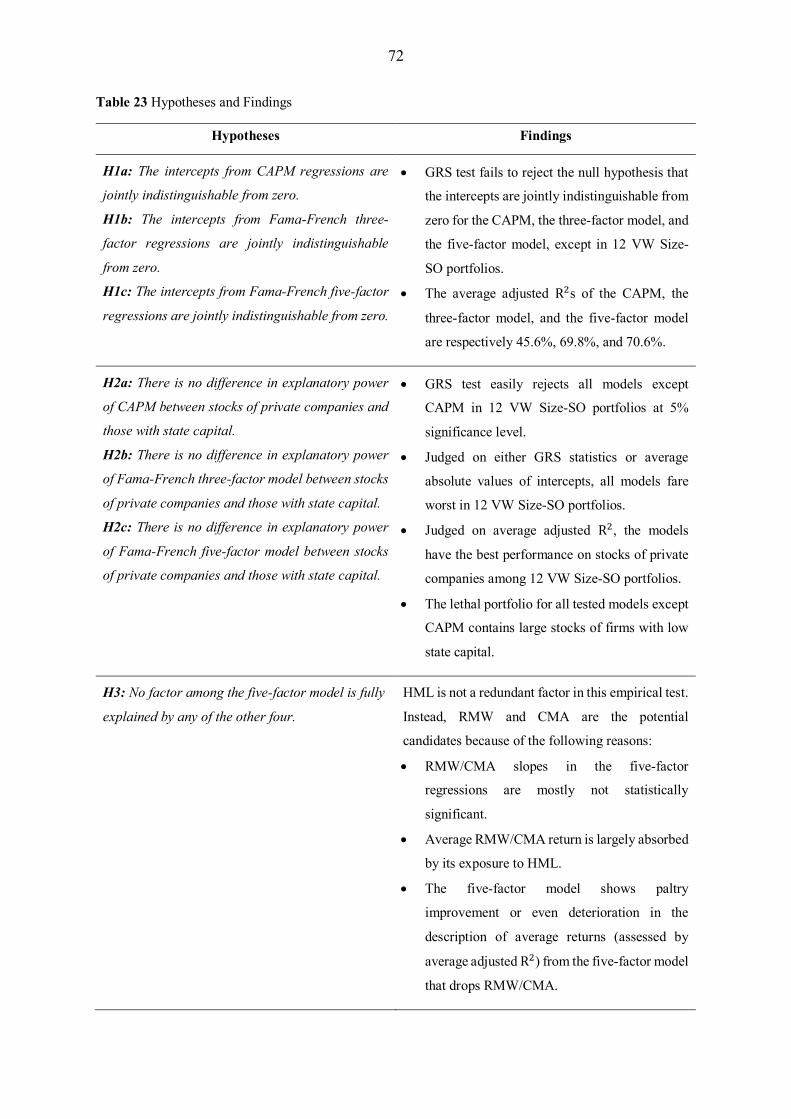
72

Table 23 Hypotheses and Findings

Hypotheses Findings

H1a: The intercepts from CAPM regressions are

jointly indistinguishable from zero.

H1b: The intercepts from Fama-French three-

factor regressions are jointly indistinguishable

from zero.

H1c: The intercepts from Fama-French five-factor

regressions are jointly indistinguishable from zero.

GRS test fails to reject the null hypothesis that

the intercepts are jointly indistinguishable from

zero for the CAPM, the three-factor model, and

the five-factor model, except in 12 VW Size-

SO portfolios.

The average adjusted R2s of the CAPM, the

three-factor model, and the five-factor model

are respectively 45.6%, 69.8%, and 70.6%.

H2a: There is no difference in explanatory power

of CAPM between stocks of private companies and

those with state capital.

H2b: There is no difference in explanatory power

of Fama-French three-factor model between stocks

of private companies and those with state capital.

H2c: There is no difference in explanatory power

of Fama-French five-factor model between stocks

of private companies and those with state capital.

GRS test easily rejects all models except

CAPM in 12 VW Size-SO portfolios at 5%

significance level.

Judged on either GRS statistics or average

absolute values of intercepts, all models fare

worst in 12 VW Size-SO portfolios.

Judged on average adjusted R2, the models

have the best performance on stocks of private

companies among 12 VW Size-SO portfolios.

The lethal portfolio for all tested models except

CAPM contains large stocks of firms with low

state capital.

H3: No factor among the five-factor model is fully

explained by any of the other four.

HML is not a redundant factor in this empirical test.

Instead, RMW and CMA are the potential

candidates because of the following reasons:

RMW/CMA slopes in the five-factor

regressions are mostly not statistically

significant.

Average RMW/CMA return is largely absorbed

by its exposure to HML.

The five-factor model shows paltry

improvement or even deterioration in the

description of average returns (assessed by

average adjusted R2) from the five-factor model

that drops RMW/CMA.

73

6.2 Limitation and Suggestion for Further Research

Like any other studies, this thesis inevitably has its own limitations. Firstly, although the period

of 102 months is considered relatively long when compared with other empirical tests in

Vietnam so far, it falls short when compared with other tests in markets around the world. For

instance, Fama and French (2015), Foye (2017), Huynh (2017), and Guo et al. (2017)

respectively cover 606 months, 324 months, 276 months, and 240 months for markets in the

US, the UK, Australia, and China. Therefore, our test period of 102 months is considered

relatively short when assessed by the typical duration of FF empirical tests, raising concerns

about the statistical power and reliability of the test. Nevertheless, this issue is difficult to avoid

since Vietnam’s stock market is currently a fledgling market with small size and young age.

As such, a longer period will enhance the test in terms of statistical power but it can cause other

problems such as data scarcity and undiversified test portfolios given the primitive stage of the

market in earlier years. This problem will be gradually lessened by further research in the future

when the market becomes more mature. Moreover, it would be interesting to extend the test to

cover the Carhart four-factor model or a six-factor model that adds the momentum factor as it

is a well-documented anomaly in various markets.

Secondly, our robustness analysis only includes test portfolios formed from size and state-

ownership status. Hence, it is unclear whether the models fall short due to some special

characteristics of equitized SOEs or any other way of forming the test portfolios rather than the

same variables used to construct the risk factors will lead to the same result. More extensive

robustness tests of factor models in Vietnam are needed to validate our conclusion. For

example, further research can examine how the models perform when test portfolios are

anomalies not explicitly targeted by design or when the risk factors are constructed differently

from the original approach.

Thirdly, our way of classifying state-ownership groups has some flaws. As mentioned earlier,

state-ownership status will be assigned into three groups based on the percentage of charter

capital that the state owns. Since ownership data on VNDirect only reflect the current situation,

current state-ownership status is used as a proxy for historical status. That is, if a company has

state capital in 2017, it will also have state capital in the past. This argument is reasonable as

we are safe to assume that the government only divests itself of state holdings. However, the

percentage of charter capital owned by the state can change during the test period and directly

affect which group the stocks will be assigned. For instance, Company A currently has 45%

state capital in 2017 and is assigned to group “Low” based on the breakpoint table (Table 5).

74

However, in 2015, Company A had 52% state capital, meaning the state has divested 7% since

2015. As such, Company A should be assigned to group “High” in 2015 but as we do not have

adequate data, it is still in group “Low” in 2015. Likewise, there are possibilities that some

firms currently assigned to group “Private” were state-owned in the past. Although we will not

be able to identify all these cases due to lack of data, there are not many of them since

equitization process has remained slow and problematic.

6.3 Concluding Remarks

This empirical test provides cautious support for the superiority of the five-factor model over

the CAPM and the three-factor model. Still, the five-factor model cannot fully explain average

returns in Vietnam’s stock market since it fails when test portfolios are formed from state

capital, which is not explicitly targeted by design. With updated data, the five-factor model can

explain 70.6% of variation in stock returns, which is lower than the average adjusted R2 levels

of previous studies in Vietnam’s stock market (e.g.: 81%-85% for the three-factor model) and

other markets. Besides, there exists a multicollinearity issue, reflected in the highly negative

correlation between HML and RMW of – 0.79. Hence, further research is essential to verify

these findings and to provide more extensive robustness analyses.

Does the five-factor model have any useful application in Vietnam’s stock market? Despite its

shortfalls, the answer is yes. Less-than-perfect models can provide meaningful descriptions of

average returns since creating an impeccable model is impossible (Fama and French, 2017).

Factor models are often used as a tool for portfolio performance evaluation, portfolio design,

and cost-of-equity estimation. Regarding the first use where abnormal returns (measured by

alphas) are the sole interest, this empirical test suggests that the three-factor model will fare

better than the CAPM and as well as the five-factor model due to the potential redundancy of

RMW and CMA. Nevertheless, if one also cares about portfolio tilts toward size, value,

profitability, and investment premiums, the five-factor model should be selected as it can

provide more useful information via its factor slopes. With respect to the third use, the ability

of the five-factor model to estimate the cost of equity is full of doubt as it is the case for other

factor models (ibid.). The reason for this argument is that standard errors of factor premium

estimates are usually substantial, let alone their time variation characteristic. On the other hand,

evaluating portfolio performance can evade part of these problems since this task does not

require the estimates of expected factor premiums.

75

After all, the Fama-French five-factor model is an empirical asset pricing model, originally

created to capture well-documented anomalies in the US stock market. Therefore, some

adjustments or even replacements in factor construction might be necessary for it to be more

applicable in Vietnam’s stock market. The findings from this empirical test suggest a quest for

a better asset pricing model for pricing Vietnamese equities.

76

7 REFERENCES

Aharoni, G., Grundy, B. & Zeng, Q. (2013) ‘Stock Returns and the Miller Modigliani

Valuation Formula: Revisiting the Fama French Analysis’ Journal of Financial Economics

110: 347-357. Retrieved from: ScienceDirect [Accessed on 15 November 2017].

Allens Linklaters (2017) Vietnamese SOE Equitisation Available from:

https://www.allens.com.au/pubs/pdf/asia/VietnamEquitisation_SOE_2017.pdf [Accessed on

24 October 2017].

Banz, R. (1981) ‘The Relationship between Return and Market Value of Common Stocks’

Journal of Financial Economics 9: 3-18.

Basu, S. (1977) ‘Investment Performance of Common Stocks in Relation to Their Price-

Earnings Ratios: A Test of the Efficient Market Hypothesis’ The Journal of Finance 32 (3):

663-682. Retrieved from: JSTOR [Accessed on 22 October 2017].

Bodie, Z., Kane, A. & Marcus, A. (2014) Investments (10th edition). US: McGraw-Hill

Education.

Bui, N. (2017) Equitization of State-Owned Enterprises in Vietnam Available from:

https://www.linkedin.com/pulse/equitization-state-owned-enterprises-vietnam-nhu-bui/

[Accessed on 24 October 2017].

Celik, S. (2012) ‘Theoretical and Empirical Review of Asset Pricing Models: A Structural

Synthesis’. International Journal of Economics and Financial Issues [Online], 2 (2). Available

from: http://www.econjournals.com/index.php/ijefi/article/view/111/pdf [Accessed on 30

October 2017].

Chiah, M., Chai, D., Zhong, A., & Li, S. (2016) ‘A Better Model? An Empirical Investigation

of the Fama-French Five-Factor Model in Australia’ International Review of Finance 16 (4):

595-638. Retrieved from: SSRN [Accessed on 30 September 2017].

Fama, E. (1970) ‘Efficient Capital Markets: A Review of Theory and Empirical Work’ The

Journal of Finance 25 (2): 383-417. Retrieved from: JSTOR [Accessed on 26 September

2017].

Fama, E. & French, K (2004) ‘The Capital Asset Pricing Model: Theory and Evidence’.

Journal of Economic Perspectives 18 (3): 25-46.

Fama, E. & French, K. (1992) ‘The Cross-Section of Expected Stock Returns’ The Journal of

Finance 47 (2): 427-465. Retrieved from: JSTOR [Accessed on 29 October 2017].

Fama, E. & French, K. (1993) ‘Common Risk Factors in the Returns on Stocks and Bonds’

Journal of Financial Economics 33: 3-56.

Fama, E. & French, K. (2006) ‘Profitability, Investment, and Average Returns’ Journal of

Financial Economics 82: 491-518. Retrieved from: ScienceDirect [Accessed on 15 November

2017].

77

Fama, E. & French, K. (2015) ‘A Five-Factor Asset Pricing Model’ Journal of Financial

Economics 116: 1-22. Retrieved from: ScienceDirect [Accessed on 30 September 2017].

Fama, E. & French, K. (2017) ‘International Tests of a Five-Factor Asset Pricing Model’

Journal of Financial Economics 123: 441-463. Retrieved from: ScienceDirect [Accessed on

30 September 2017].

Foye, J. (2017) Testing Alternative Versions of the Fama-French Five-Factor Model in the UK

Available from: https://papers.ssrn.com/sol3/papers.cfm?abstract_id=3020947 [Accessed on

30 September 2017].

Guo, B., Zhang, W., Zhang, Y. & Zhang, H. (2017) ‘The Five-Factor Asset Pricing Model

Tests for the Chinese Stock Market’ Pacific-Basin Finance Journal 43: 84-106. Retrieved

from: ScienceDirect [Accessed on 05 January 2018].

Ha, M (2017) Nghich ly co phan hoa doanh nghiep nha nuoc (SOE Equitization Paradox)

Available from: http://vneconomy.vn/thoi-su/nghich-ly-co-phan-hoa-doanh-nghiep-nha-nuoc-

2017090809461727.htm [Accessed on 24 October 2017].

Hang Nguyen & Hiep Nguyen (2012) Kiem dinh mo hinh Fama – French tai thi truong chung

khoan Viet Nam (Empirical test of Fama – French model in Vietnam’s stock market).

HNX Index List (n.d.) Available from: www.hnx.vn/co-phieu-etfs/danh-muc-chi-so.html

[Accessed on 23 October 2017].

HOSE Market Cap List (n.d.) Available from:

www.hsx.vn/Modules/Rsde/Web/Index?fid=fd391fb3864946edb5f95002753ac850 [Accessed

on 23 October 2017].

Huberman, G. & Kandel, S. (1987) ‘Mean-variance Spanning’ Journal of Finance 42: 873–

888.

Huu, H. (2017) Se tang cuong giai phap thuc day su minh bach (Solutions to promote

transparency will be strengthened) Available from: http://tinnhanhchungkhoan.vn/chung-

khoan/se-tang-cuong-giai-phap-thuc-day-su-minh-bach-196211.html [Accessed on 24

October 2017].

Huynh, T. (2017) ‘Explaining Anomalies in Australia with a Five-Factor Asset Pricing Model’

International Review of Finance 18 (1): 123-135. Retrieved from: SSRN [Accessed on 30

September 2017].

Le, C. (2015) The Fama – French Factors: Evidence from the Vietnamese Stock Market

Available from: https://papers.ssrn.com/sol3/papers.cfm?abstract_id=2610588 [Accessed on

30 September 2017].

78

Market Capitalization of Listed Domestic Companies (% of GDP) Available from:

https://data.worldbank.org/indicator/CM.MKT.LCAP.GD.ZS [Accessed on 23 October 2017].

Markowitz, H. (1952) ‘Portfolio Selection’ The Journal of Finance, 7 (1): 77-91. Retrieved

from: JSTOR [Accessed on 22 October 2017].

Miller, T., Dolvin, S. & Jordan, B. (2011) Fundamentals of Investments: Valuation and

Management (6th edition). US: McGraw-Hill Companies.

Nguyen, N., Ulku, N. & Zhang, J. (2015) The Fama – French Five Factor Model: Evidence

from Vietnam Available from: https://www.nzfc.ac.nz/archives/2016/papers/updated/49.pdf

[Accessed on 30 September 2017].

Nguyen, P. & Tran, H. (2012) ‘Applying Fama and French Three Factors Model and Capital

Asset Pricing Model in the Stock Exchange of Vietnam’ International Research Journal of

Finance and Economics 95: 115-120.

Novy-Marx, R. (2013) ‘The Other Side of Value: The Gross Profitability Premium’ Journal of

Financial Economics 108: 1-28. Retrieved from: ScienceDirect [Accessed on 15 November

2017].

OECD (2016) State-Owned Enterprises in Asia: National Practices for Performance

Evaluation and Management Available from: https://www.oecd.org/corporate/SOEs-Asia-

Performance-Evaluation-Management.pdf [Accessed on 24 October 2017].

PM Speeds up SOEs Restructuring (2017) Available from:

http://vietnamnews.vn/economy/350670/pm-speeds-up-soes-

restructuring.html#szgUrCbOFlle61C1.97 [Accessed on 24 October 2017].

Reinganum, M. (1981) ‘Misspecification of Capital Asset Pricing: Empirical Anomalies Based

on Earnings’ Yields and Market Values’ Journal of Financial Economics 9: 19-46.

Rosenberg, B., Reid, K. & Lanstein, R. (1985) ‘Persuasive Evidence of Market Efficiency’

Journal of Portfolio Management 11 (3): 9-16.

Schwert, G. (2003) ‘Anomalies and Market Efficiency’ In: Constantinides, G., Harris, M. &

Stulz, R. (ed.) Handbook of the Economics of Finance. Elsevier B.V.

Sharpe, W. (1964) ‘Capital Asset Prices: A Theory of Market Equilibrium under Conditions

of Risk’. The Journal of Finance 19 (3): 425-442. Retrieved from: JSTOR [Accessed on 16

October 2017].

SOE Restructuring Must Be More Efficient: Experts (2017) Available from:

http://vietnamnews.vn/economy/381228/soe-restructuring-must-be-more-efficient-

experts.html#6BLkhoTVkmXFOMG6.97 [Accessed on 24 October 2017].

Thi truong chung khoan 2017 co quy mo von hoa tren 70% GDP, vuot muc tieu den 2020

(2017) (Stock market capitalization above 70% of GDP in 2017, surpass 2020 target) Available

from: https://vietstock.vn/2017/12/thi-truong-chung-khoan-2017-co-quy-mo-von-hoa-tren-

70-gdp-vuot-muc-tieu-den-2020-830-573293.htm [Accessed on 27 January 2018].

79

Thuong, G. (2017) Thao tung gia co phieu, mot ca nhan bi phat 550 trieu dong (Stock price

manipulation, an individual was fined 550 million Vietnam dong) Available from:

https://www.baomoi.com/thao-tung-gia-co-phieu-mot-ca-nhan-bi-phat-550-trieu-

dong/c/23205502.epi [Accessed on 24 October 2017]..

VN-Index Technical Chart (n.d.) Available from: www.vndirect.com.vn/portal/bieu-do-ky-

thuat/vnindex.shtml?request_locale=en_GB [Accessed on 23 October 2017].

Vuong, Q. & Ho, H. (2008) Mo hinh Fama – French: Mot nghien cuu thuc nghiem doi voi thi

truong chung khoan Viet Nam (Fama – French model: An empirical test regarding Vietnam’s

stock market).

80

8 APPENDICES

Appendix A

List of Illustrative Figures for the Literature Review

Figure A1 Different forms of Efficient Market (Adapted from: Miller, Dolvin, and Jordan, 2011)

Figure A2 Markowitz's Efficient Frontier (Adapted from: Bodie et al., 2014)

Figure A3 Capital Market Line and Efficient Frontier (Adapted from: Bodie et al., 2014)

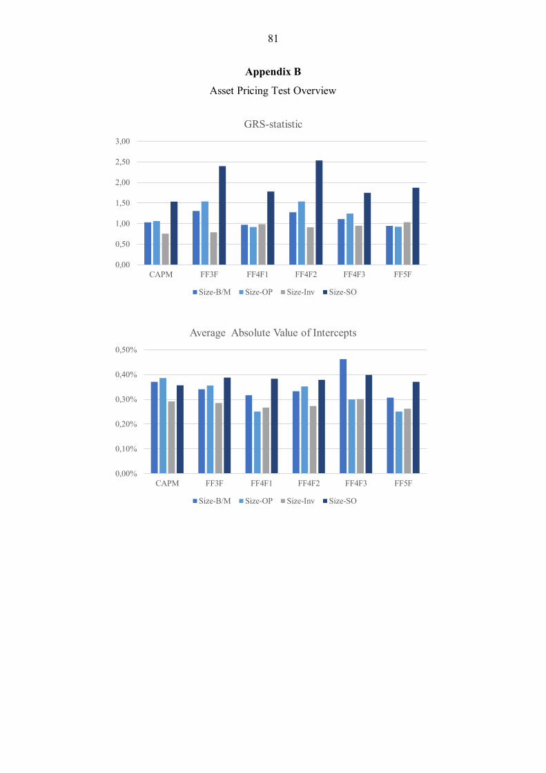
81

Appendix B

Asset Pricing Test Overview

0,00

0,50

1,00

1,50

2,00

2,50

3,00

CAPM FF3F FF4F1 FF4F2 FF4F3 FF5F

GRS-statistic

Size-B/M Size-OP Size-Inv Size-SO

0,00%

0,10%

0,20%

0,30%

0,40%

0,50%

CAPM FF3F FF4F1 FF4F2 FF4F3 FF5F

Average Absolute Value of Intercepts


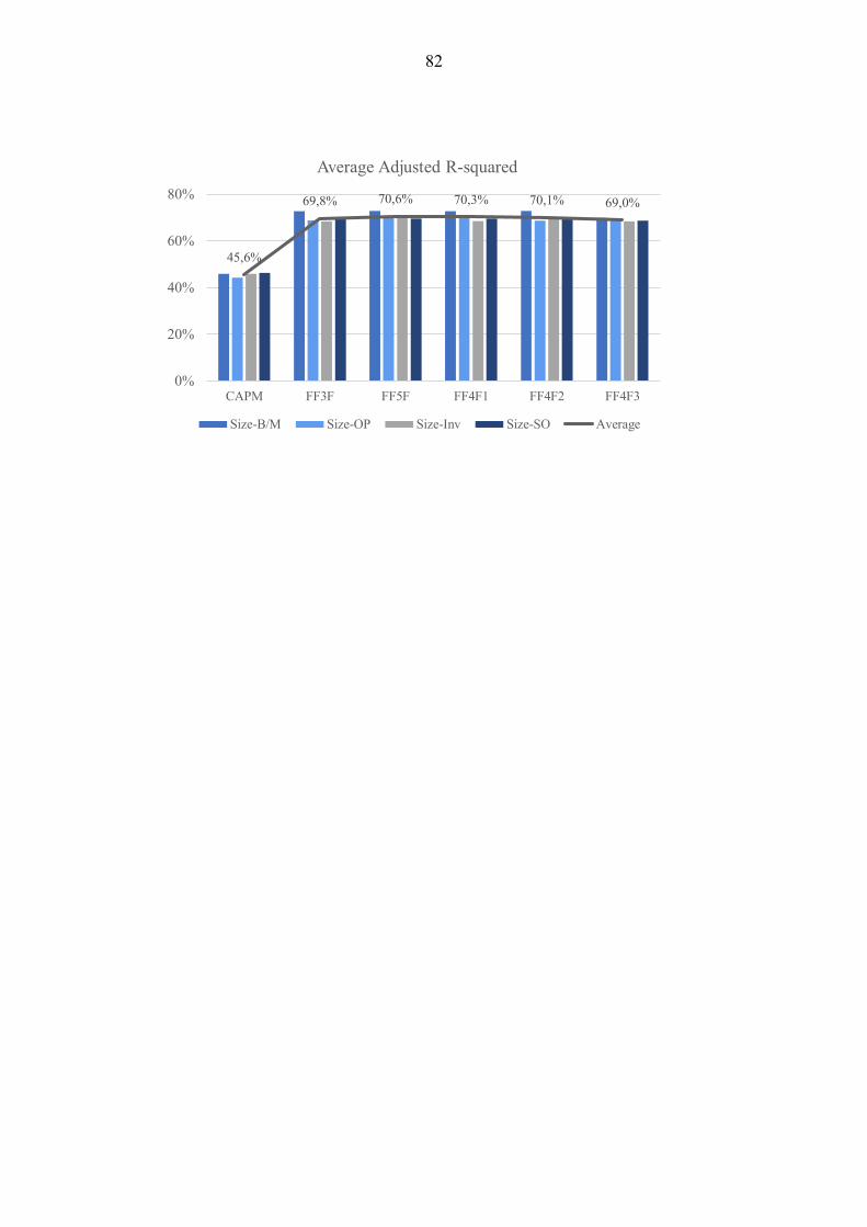
82

45,6%

69,8% 70,6% 70,3% 70,1% 69,0%

0%

20%

40%

60%

80%

CAPM FF3F FF5F FF4F1 FF4F2 FF4F3

Average Adjusted R-squared

Size-B/M Size-OP Size-Inv Size-SO Average

83

Appendix C

Adjusted R-squared across three asset pricing models (CAPM, FF three-factor, FF five-

factor) and 60 VW test portfolios

0%

20%

40%

60%

80%

100%

Lo

w 2 3

Hig

h

Wea

k 2 3

Ro

bu

st

Co

ns. 2 3

Agg

r.

Pri

vat

e

Lo

w

Hig

h


CAPM Adjusted R-squared across 60 VW test portfolios

Small 2nd size quartile 3rd size quartile Big

0%

20%

40%

60%

80%

100%

Low 2 3

Hig

h

Wea

k 2 3

Robust

Cons. 2 3

Aggr.

Pri

vat

e

Low

Hig

h


FF3F Adjusted R-squared across 60 VW test portfolios


84

0%

20%

40%

60%

80%

100%

Lo

w 2 3

Hig

h

Wea

k 2 3

Ro

bu

st

Co

ns. 2 3

Agg

r.

Pri

vat

e

Lo

w

Hig

h


FF5F Adjusted R-squared across 60 VW test portfolios


An Empirical Test of the Fama-French Five-Factor …...AN EMPIRICAL TEST OF THE FAMA-FRENCH...

Documents

Transcript of An Empirical Test of the Fama-French Five-Factor …...AN EMPIRICAL TEST OF THE FAMA-FRENCH...