An Empirical Model of Intra-HouseholdAllocations and the Marriage Market∗

Eugene ChooUniversity of Calgary

Shannon SeitzBoston College andQueen’s University

Aloysius SiowUniversity of Toronto

December 11, 2007

Abstract

We develop an empirical collective matching model with endoge-nous marriage formation, participation, and labor supply decisions.The sharing rule in our collective matching model arises endogenouslyas a transfer that clears the marriage market. With information onat least two independent marriage markets, incorporating matching inthe collective model allows us to identify the sharing rule from obser-vations on marriage decisions, regardless of the labor supply decisionsof wives and husbands. For couples in which both partners work, in-troducing the marriage market in the collective model generates a setof over-identifying restrictions that allow us to test whether the shar-ing rule that rationalizes labor supplies is consistent with the sharingrule that clears the marriage market. We estimate the sharing ruleusing 2000 Census data and implement a semi-parametric test of theover-identifying restrictions.

∗We would like to thank Karim Chalak, Peter Gottschalk, Arthur Lewbel, seminarparticipants at Duke, New York University, the University of Connecticut, and the 2007Analytical Labor Economics Conference at the University of Chicago for many helpfulcomments. Seitz gratefully acknowledges the support of the Social Sciences and Humani-ties Research Council of Canada.

1 Introduction

The unitary model of the household, long the standard for analyzing house-hold behavior, has been replaced by the collective model of Chiappori (1988,1992) in recent years. The reason for the success of the collective model istwofold. First, the collective model is appealing on theoretical grounds. Theunitary model assumes household members act as if they share a commonset of preferences. In contrast, men and women retain distinct and poten-tially conflicting individual preferences following marriage in the collectivemodel. The second reason for the success of the collective model is that alarge body of empirical evidence consistently finds the restrictions impliedby the unitary model are rejected while those implied by the collective modelare not.1

Within the collective model, the resource allocation process is summarizedby the sharing rule, a lump sum transfer of non-labor income within thehousehold, taken as given by couples when household allocations are chosen.Under a minimal set of assumptions it is possible to uncover preferences aswell as the sharing rule, up to an additive constant, from observations onlabor supplies.2 This is an extremely useful result and allows the researcherto gain valuable insight into the inner workings of the household. However,the basic collective model restricts attention to currently married couplesand is silent on other important questions such as: Why do some marriagesform and not others? Where does the sharing rule come from? As stated byLundberg and Pollak (1996):

Models that analyze bargaining within existing marriages cangive only an incomplete picture of the determinants of the well-being of men and women. The marriage market is an impor-tant determinant of distribution between men and women. At aminimum, the marriage market determines who marries and whomarries whom.

The above quotation suggests that empirical models of intra-household al-locations in existing marriages are well developed. The next question to be

1A partial list includes Lundberg (1988), Thomas (1990), Fortin and Lacroix (1997),Chiappori, Fortin, and Lacroix (2002), and Duflo (2003).

2The standard identifying assumptions in the collective model are that household allo-cations are Pareto efficient and preferences are egoistic or caring. For further details, seeBrowning and Chiappori (1998) and Chiappori and Ekelund (2002).

1

addressed in this research program is clear: how do we empirically investigatemarriage matching with intra-household allocations? Our paper representsone step in this direction.

The goal of this paper is to develop an empirical framework for analyzingboth marriage matching and the intra-household allocation of resources. Aprimary criteria in this development is that the empirical framework delib-erately minimizes restrictions on observed behavior. To this end, we take asour starting point Chiappori’s (1992) collective model of intra-household al-locations. Standard assumptions, Pareto efficiency and egoistic preferences,from the collective framework are maintained and no additional assumptionsare imposed on the intra-household problem for married couples. We thenembed the collective model in the marriage matching model of Choo and Siow(2006; hereafter CS). Within CS, utility is transferable and equilibrium trans-fers clear the marriage market. The model of CS produces a nonparametricmatching function that is consistent with any observed marriage matchingpattern in a single marriage market. Together, the collective model and themodel of CS produce a flexible empirical model of marriage and householdlabor supply.

From the collective matching model, we derive a sharing rule that isthe equilibrium outcome of marriage matching. In contrast to the standardcollective framework, our theory on marriage matching produces an exactfunctional form for the sharing rule. Analogous to Chiappori, Fortin, andLacroix (2002; hereafter CFL), the sharing rule in our framework depends on‘distribution factors,’ factors that affect household allocations only throughthe sharing rule (they do not directly affect preferences or the budget set).As in CFL, the distribution factors in our sharing rule are characteristicsthat determine one’s outside options in the marriage market, including thestocks of men and women with the same characteristics as the husband andwife, respectively, in the market. We thus provide a formal justificationfor intra-household transfers that depend on marriage market conditions.Our equilibrium sharing rule is also a function of the wages and populationsupplies of all other types of men and women that are available in other typesof matches. Thus, our model generates a sharing rule with many distributionfactors.

Our framework is very flexible. We allow preferences and marital pro-duction technologies to vary depending on the participation status of thewife and on the characteristics of both spouses. Our framework also providesa convenient way to model marriage decisions in combination with discrete

2

and/or continuous labor supply decisions for married men and women.3 Inour application, it is assumed husbands choose continuous hours and wives ei-ther choose continuous hours or not to work. A natural interpretation of thisset-up is that individuals choose whether to enter ‘specialized’ (non-workingwife) or ‘non-specialized’ (working wife) marriages. Our framework can bereadily extended to cases where one or both spouses are not working. As wedemonstrate below, identification of the sharing rule does not rely upon onvariation in labor supplies within married households in our framework.

We establish identification of all of the structural parameters analytically.Identification in our framework is therefore completely transparent. We show:

1. Identification of the collective model is exactly the same as in CFLfor couples in non-specialized marriages. In this instance, the sharingrule can be identified up to an additive constant from observations onlabor supply. What is new in our framework is that the sharing rulecan also be identified independently from the marriage decision. As aresult, our framework generates over-identifying restrictions that allowus to test whether the sharing rule arising from the marriage market isconsistent with the sharing rule that determines labor supplies withinmarried households. The goal of our empirical analysis will be to testthese restrictions.

2. With information on at least two independent marriage markets, onecan non-parametrically identify the sharing rule from observations onmarriage decisions, regardless of the labor supply decisions of wivesand husbands. The introduction of information on marriage decisionsis crucial for identification in the case where one or both spouses arenot working, as information on behavior within the household is limitedwhen there is no variation in household labor supply.4

We are able to identify all of the structural parameters of interest. As aresult, our model is both flexible and at the same time amenable to policyanalysis.

We estimate the collective matching model for non-specialized couplesusing data from the 2000 United States Census. After estimating the model,

3Blundell, Chiappori, Magnac and Meghir (2007), Vermeulen (2006), and Lise andSeitz (2007) present collective models in which one or both spouses do not work full time.

4Our result can be generalized to any discrete choice of hours, including zero hours,part-time and full-time work.

3

we test the restrictions on labor supplies and marriage decisions implied bythe collective matching model. As pointed out by Blundell, Browning, andCrawford (2003) in a related context, a rejection of the collective frameworkusing parametric tests could arise due to a failure of the collective modelitself or to functional form misspecification of preferences. To this end, weformulate a semi-parametric test of our collective model which involves com-paring the partial derivatives of the sharing rule from labor supplies to thosefrom marriage decisions.5 The results indicate coming soon...

The remainder of the paper is organized as follows. We survey the relatedliterature in Section 2. In Section 3, we describe our benchmark version ofthe collective model and Section 4 describes the marriage market and theequilibrium. In Section 5, we establish conditions under which the structuralparameters of the model (preference parameters and the sharing rule) areidentified. In Section 6 we show how the restrictions of our model can betested nonparametrically. We nonparametrically estimate our model usingdata from the 2000 Census and present the estimation results in Section 7.Section 8 concludes.

2 Related Literature

We are indebted to a large literature. The study of intra-household alloca-tions began with, among others, Becker (1973, 1994; summarized in 1991),the bargaining models of Manser and Brown (1980) and McElroy and Horney(1981), McElroy (1990) and the collective model of Chiappori (1988, 1992).A related literature, encompassing a diverse set of models, has studied thelink between marriage market conditions and marriage rates. Becker (1973)was the first to consider the relationship between sex ratios and marriagerates. Brien (1997) tests the ability of several measures of marriage marketconditions to explain racial differences in marriage rates. The link betweensex ratios and household outcomes was also extended to the labor supplydecision. Grossbard-Schectman (1984) constructs a model where more favor-able conditions in the marriage market improve the bargaining position of

5It should be emphasized that our identification results are still parametric in the sensethat some assumptions on the functional form of preferences are imposed, namely thatpreferences are egoistic. Chiappori (1988) develops non-parametric identification resultsfor the collective model. In recent work, Vermeulen et al. (2007) extend the results ofChiappori to a collective framework with externalities and public goods.

4

individuals within marriage. One implication of Grossbard-Schectman andrelated models that has been tested extensively in the literature is that, forexample, an improvement in marriage market conditions for women trans-lates into a greater allocation of household resources towards women, whichhas a direct income effect on labor supply. Tests of this hypothesis have re-ceived support in the literature (see among others, Becker, 1981; Grossbard-Schectman, 1984, 1993; Grossbard-Schectman and Granger, 1998; Chiappori,Fortin, and Lacroix, 2002; Seitz, 2004; Grossbard and Amuedo-Dorantes,2007). Our empirical work considers the link between the sex ratio and bothmarriage and labor supply decisions in a general version of the collectivemodel with matching.

Several important predecessors of our work integrate the collective modeland the marriage market (Becker and Murphy, 2000; Browning, Chiapporiand Weiss, 2003) and extend the integrated model to consider pre-maritalinvestments (Chiappori, Iyigun, and Weiss, 2006; Iyigun and Walsh, 2007).In these integrated collective models and in our work the sharing rule arisesendogenously in the marriage market. Our paper differs from this recentwork in focus. Our goal is to develop an empirical framework that minimizesa priori restrictions on marriage matching and labor supply patterns. In thisrespect, our empirical framework can be used to test some of the qualitativepredictions of the existing integrated models.

Our treatment of discrete labor supply choices within the collective model,while different in formulation, was influenced by the work of Blundell, Chi-appori, Magnac, and Meghir (2007). Blundell, et al. (2007) establish iden-tification of the collective model in the case where the labor supply decisionof one spouse is discrete and of the other spouse is continuous. In contrastto Blundell et al. (2007), information on marriage behavior can be usedto identify the sharing rule in our framework, even in the case where bothhousehold members are not working.

Our static model is restrictive. We assume spouses have access to bind-ing marital agreements and there is no divorce. There is an active empiricalliterature studying dynamic intra-household allocations and marital behav-ior. Seitz (2004) constructs and estimates a dynamic model in which thesex ratio, marriage, and employment decisions are jointly determined. Shefinds that variation in the ratio of single men to single women across race canexplain much of the black-white differences in marriage and employment inthe US. Brien, Lillard, and Stern (2006) estimate a dynamic model of cohab-itation, and divorce where individuals learn about the quality of their match

5

over time. Del Boca and Flinn (2006a, 2006b) estimate models of householdlabor supply where the household members can choose to interact in eithera cooperative or a noncooperative fashion. Mazzocco and Yamaguchi (2006)study savings, marriage, and labor supply decisions in a collective frame-work, in which an individual’s weight in the household’s allocation processdepends on the outside options of each spouse, in this case, divorce. Chooand Siow (2005) estimate a dynamic nonparametric matching model. Ourfocus here is on developing and estimating an empirical model of intrahouse-hold allocations and matching that imposes a minimal set of assumptions.Incorporating dynamics in our framework in the spirit of Choo and Siow(2005) is an important extension left to future work.

3 The Collective Model

Consider a society that is composed of many segmented marriage markets.For expositional ease, assume there is one type of man and one type of womanwithin each society. We extend our analysis to multiple types in the empiricalanalysis described in Section 6. All men and women within the same markethave the same ex-ante opportunities and preferences. Let m be the numberof men and f be the number of women within a market.

Decisions are made within the model in two stages. In the first stage,individuals choose whether to marry and whether the wife works within themarriage. We refer to marriages in which the wife does not work in the labormarket as specialized marriages (s) and marriages in which both spouses workas non-specialized marriages (n). The index k, k ∈ {n, s} describes whethera married couple is non-specialized or specialized.6 In the second stage, laborsupply decisions for working spouses and consumption allocations are chosen.For simplicity, all men and all unmarried women are assumed to have positivehours of work.

3.1 Preferences

Let C and c be the private consumption of women and men, respectively, andH and h denote their respective labor supplies. Preferences are described by:

Uk(C, 1−H) + Γk + εk

6It is straightforward to extend our model to the case where neither partner works.

6

for married women and

uk(c, 1− h) + γk + εk

for married men. For both spouses, the first term is defined over consumptionand leisure and affects the intrahousehold allocation. The last two terms, asin CS, affect marriage behavior but do not directly influence the intrahouse-hold allocation.

The parameters Γk and γk capture invariant gains to a marriage of typek for wives and husbands, respectively and are assumed to be separablefrom consumption and leisure.7 Idiosyncratic type I extreme value preferenceshocks, εk and εk, are realized before marriage decisions are made. It isassumed that the preference shocks do not depend on the specific identity ofthe spouse.

3.2 Intrahousehold allocations

We begin by considering the second stage intrahousehold decision process.This is the familiar setting of the collective model, first developed by Chiap-pori (1988, 1992). We consider in turn the intra-household allocation problemfor singles, non-specialized and specialized couples.

3.2.1 Singles

The problem facing a single woman is:

max{C,H}

U0(C, 1−H) + Γ0 + ε0 (S)

subject to the budget constraint

C ≤ W0H + A0

and likewise for a single man:

max{c,h}

u0(c, 1− h) + γ0 + ε0

subject to the budget constraint

c ≤ w0h + a0

7As in CS, invariant gains to marriage allow the model to fit the observed marriagematching patterns in the data.

7

3.2.2 Non-specialized couples

Consider a husband and wife in a couple where both partners work. Totalnon-labor family income, denoted A, and wages for the husband w and wifeW are realized before marriage decisions are made. The social planner’sproblem for the household is:

max{c,C,h,H}

Un(C, L) + Γn + εn + ωn

[un(c, l) + γn + εn

](PN)

subject to the family budget constraint:

c + C ≤ A + WH + wh

where the Pareto weight on the husband’s utility in non-specialized marriagesis ωn.

A major insight of Chiappori (1988) is that, if household decisions arePareto efficient, the above program can be decentralized subject to a lumpsum transfer or sharing rule, denoted τn(W,w, A,R). At present, we conjec-ture that the sharing rule is of a form similar to that in CFL: transfers dependon wages, nonlabor income, and a set of ‘distribution factors’ R, which con-tains labor and marriage market conditions for all the possible matches anindividual could have entered. The decentralized problem for the wife in thesecond stage is:

max{C,L}

Un(C,L)

subject to C ≤ WH + τn(W,w,A,R)

and the problem facing husbands in the second stage is:

max{c,l}

un(c, l)

subject to c ≤ wh + A− τn(W,w,A,R)

The sharing rule in the decentralized problem, and the Pareto weights inthe social planner’s problem, are treated as pre-determined at the point con-sumption and leisure allocations are chosen. The large literature on collectivemodels is, with few exceptions, agnostic regarding the origins of the sharingrule. A central focus of our paper is to derive a sharing rule from mar-riage market clearing. In Section 4.1, we show that marriage market clearinggenerates a sharing rule of precisely the form presented here.

8

3.2.3 Specialized couples

For households in which the wife does not work, the social planner’s problemis:

max{c,C,h}

Us(C, 1) + Γs + εs + ωs

[us(c, l) + γs + εs

](PS)

subject to the family budget constraint:

c + C ≤ A + w(1− h)

where the Pareto weight on the husband’s utility in specialized marriages isωs. The decentralized problem for the husband is

max{c,l}

us(c, l, εg)

subject to c ≤ wh + A− τs(w, A,R)

and the wife simply receives Us(C, 1), where C = τs(w,A,R). Since the wifeis not working, the Pareto weight in specialized marriages only depends onthe husband’s wage, non-labor income, and the distribution factors.8

3.3 The marriage decision

In the first period, agents decide whether to marry and whether to specialize.Once the idiosyncratic gains from marriage, εk and εk, are realized, individ-uals choose the household structure that maximizes utility. Individuals havethree alternatives: remain single, enter a specialized marriage, or enter anon-specialized marriage. For women, the indirect utility from remainingsingle is:

V0(ε0) = Q0[W0, Y0] + Γ0 + ε0

from entering a specialized marriage is:

Vs(εs) = Qs[Ys] + Γs + εs

and from entering a non-specialized marriage is:

Vn(εn) = Qn[W,Yn] + Γn + εn

8Although individual types have been suppressed here for convenience, the sharing rulewill in general depend on characteristics of both spouses and also on the society in whichthe couple resides.

9

where

Ys = τs(w, A,R)

Yn = τn(W,w, A,R)

The functions Q0[W0, Y0], Qs[Ys], and Qn[W,Yn] are the indirect utilitiesresulting from the second stage consumption and labor supply decisions.Given the realizations of ε0, εn, and εs, she will choose the marital choicewhich maximizes her utility. The utility from her optimal choice will satisfy:

V ∗(ε0, εs, εn) = max[V0(ε0), Vs(εs), Vn(εn)] (1)

The problem facing men in the first stage is analogous to that of women.Given the realizations of ε0, εn, and εs, he will choose the marital choicewhich maximizes utility. The indirect utility from remaining single is:

v0(ε0) = q0[w0, y0] + γ0 + ε0

from entering a specialized marriage is:

vs(εs) = qs[w, ys] + γs + εs

and from entering a non-specialized marriage is:

vn(εn) = qn[w, yn] + γn + εn

where

ys = A− τs(w, A,R)

yn = A− τn(W,w, A,R)

and the q0[w0, y0], qs[w, ys], and qn[w, yn] are the indirect utilities from thehousehold’s problem in the second stage. Given the realizations of ε0, εn, andεs, he will choose the marital choice which maximizes his utility. The utilityfrom his optimal choice will therefore satisfy:

v∗(ε0, εs, εn) = max[v0(ε0), vs(εs), vn(εn)] (2)

10

4 The Marriage Market

In this section, we construct supply and demand conditions in the marriagemarket and define an equilibrium for this market. Our model of the marriagemarket closely follows CS. Assume that there are many women and men inthe marriage market, each woman is solving (1) and each man is solving (2).Under the assumption εk and εk are i.i.d. extreme value random variables,McFadden (1974) shows that, within a market, the number of marriagesrelative to the number of females can be expressed as the probability womenprefer entering a type k marriage relative to all other alternatives, includingremaining single:

Πk

f=

exp(Γk + Qk[·]

)

∑l∈{0,s,n} exp

(Γl + Ql[·]

) (3)

where Πk is the number of marriages of type k. Similarly, for every man

πk

m=

exp(γk + qk[·]

)

∑l∈{0,s,n} exp

(γl + ql[·]

) (4)

where πk is the number of marriages of type k.Equations (3) and (4) imply the following supply and demand equations:

ln Πk − ln Π0 = (Γk − Γ0) + Qk[·]−Q0[W0, Y0] (5)

where Π0 is the number of females who choose to remain unmarried, and

ln πk − ln π0 = (γk − γ0) + qk[w, yk]− q0[w0, y0] (6)

and π0 is the number of males who choose to remain unmarried. CS call theleft hand side of (5) the net gains to a k type marriage relative to remainingunmarried for women and the left hand side of (6) the net gains to a k typemarriage relative to remaining unmarried for men.

Marriage market clearing requires the supply of wives to be equal to thedemand for wives for each type of marriage:

Πk = πk = Π∗k ∀ k. (7)

The following feasibility constraints ensure that the stocks of married andsingle agents of each gender and type do not exceed the aggregate stocks of

11

agents of each gender in the market:

f = Π0 +∑

k

Π∗k (8)

m = π0 +∑

k

Π∗k. (9)

We can now define a rational expectations equilibrium. There are two partsto the equilibrium, corresponding to the two stages at which decisions aremade by the agents. The first corresponds to decisions made in the marriagemarket; the second to the intra-household allocation. In equilibrium, agentsmake marital status decisions optimally, the sharing rules clear each marriagemarket, and conditional on the sharing rules, agents choose consumption andlabor supply optimally. Formally:

Definition 1 A rational expectations equilibrium consists of a distribution ofmales and females across marital status and type of marriage {Π0 , π0, Π∗

k},a set of decision rules for marriage {V ∗(ε0G, εsG, εnG), v∗(ε0g, εsg, εng)}, a set

of decision rules for spousal consumption and leisure {C0, Cn, c0, ck, L0, Ln,l0, lk}, exogenous marriage and labor market conditions W,w,A,R and a setof transfers {τk(·)} such that:

1. The decision rules {V ∗(·), v∗(·)} solve (1) and (2);

2. All marriage markets clear implying (7), (8), (9) hold;

3. For a type n marriage, the decision rules {Cn, cn, Ln, ln} solve (PN);

4. For a type s marriage, the decision rules {cs, ls} solve (PS).

Theorem 2 A rational expectations equilibrium exists.

Sketch of proof: We have already demonstrated 1, 3, and 4. We next needto show that there is a set of transfers, {τn, τs} which clears the marriagemarket. Let τ be the vector of transfers. For every type of marriage k in themarriage market, define the excess demand function for marriages by men:

Ek(τ) = πk(τ)− Πk(τ). (10)

12

The demand and supply functions (3) and (4) satisfy the weak gross sub-stitute property for every marriage market. So the excess demand functionsalso satisfy the weak gross substitute property.9

The equilibrium stocks of marriages of each type, as well as the stocks ofsingles of each type, will depend on wages and non-labor incomes, as well aslabor and marriage market conditions across all alternatives, summarized byR, and are denoted:

Π∗k(W,w,A,R)

Π∗0(W,w,A,R)

π∗0(W,w, A,R)

Remark: In monogamous marriage markets, where different types of spousesare substitutes for each other (since an individual can at most marry onetype), the weak gross substitute property is generic. Thus existence of mar-riage market equilibrium is more general than our specific random utilitymodel for spousal choice, which we use for empirical convenience. Kelsoand Crawford (1982) were the first to use the gross substitute property todemonstrate existence in matching models.

4.1 Derivation of the sharing rule

In this section, we show that sharing rules arise endogenously as the transfersthat clear the marriage market. Recall, the demand and supply conditionscan be expressed as:

ln Πk − ln Π0 = (Γk − Γ0) + Qk[·]−Q0[W0, Y0]

andln πk − ln π0 = (γk − γ0) + qk[·]− q0[w0, y0]

respectively. Marriage market clearing requires Πk = πk which implies

ln T = ln Γn − ln γn + Qn[W, τn(W,w, A,R)]

−Q0[W0, Y0]− qn[w, A− τn(W,w, A,R)] + q0[w0, y0] (11)

9Mas-Colell, Winston and Green (1995: p. 646, exercise 17.F.16C) provide a proofof existence of market equilibrium when the excess demand functions satisfy the weakgross substitute property. For convenience, we reproduce their proof in our context inAppendix B. The proof does not rely on Walras Law or that excess demand is homogenousof degree zero in τ , neither of which are satisfied by our model.

13

for non-specialized couples, and

ln T = ln Γs − ln γs + Qs[τs(w, A,R)]

−Q0[W0, Y0]− qs[w, A− τs(w, A,R)] + q0[w0, y0] (12)

for specialized couples, where ln Γk = Γk − Γ0 and ln γk = γk − γ0. Equa-tions (11) and (12) can be solved for τn and τs as a function of wages, non-labor incomes and market tightness. The resulting sharing rules are used inthe second stage household problem as outlined in Section 3.

5 Identification

In this section, we demonstrate how information on spousal labor suppliesand on marriage decisions can be used to identify the preferences of individualhousehold members as well as the sharing rule.

5.1 Non-specialized couples

5.1.1 Labor supply

Consider couples in which both partners work strictly positive hours. Assumethat the unrestricted labor supplies for husbands and wives, Hn(W,w,A,R)and hn(W,w,A,R) are continuously differentiable. The Marshallian laborsupply functions associated with the collective framework are related to thereduced form according to:

Hn(W,w, A,R) = Hn[W, τn(W,w, A,R)] (13)

hn(W,w, A,R) = hn[w, A− τn(W,w,A,R)] (14)

This is exactly the setting of CFL. As in CFL, it is straightforward to showthat the partial derivatives of the sharing rule can be recovered from laborsupplies. For completeness, we reproduce the identification results of CFLhere. Suppose for simplicity that R has one element, r. Define B1 = hnW

hnA,

D1 = hnr

hnr, E1 = Hnw

HnA, and F1 = Hnr

HnA. The following proposition outlines the

necessary and sufficient conditions for identification of the sharing rule.

Proposition 3 Take any point such that HnA · hnA 6= 0. Then: (i) If thereexists exactly one distribution factor r such that D1 6= F1, the following

14

conditions are necessary for any pair (H(·), h(·)) to be solutions of (PN) forsome sharing rule τn(W,w, A, r):

∂

∂r

( D1

D1 − F1

)=

∂

∂A

( D1F1

D1 − F1

)

∂

∂W

( D1

D1 − F1

)=

∂

∂A

( B1F1

D1 − F1

)

∂

∂w

( D1

D1 − F1

)=

∂

∂A

( D1E1

D1 − F1

)

∂

∂W

( D1F1

D1 − F1

)=

∂

∂r

( B1F1

D1 − F1

)

∂

∂w

( D1F1

D1 − F1

)=

∂

∂r

( D1E1

D1 − F1

)

∂

∂w

( B1F1

D1 − F1

)=

∂

∂W

( D1E1

D1 − F1

)

HnW −HnA

(Hn +

B1F1

D1 − F1

)(D1 − F1

D1

)≥ 0

hnw − hnA

(hn − D1E1

D1 − F1

)(−D1 − F1

F1

)≥ 0

(ii) Under the assumption that the conditions in (i) hold, the sharing rule isdefined up to an additive constant κ. The partial derivatives of the sharingrule are given by:

τnA =D1

D1 − F1

τnr =D1F1

D1 − F1

τnW =B1F1

D1 − F1

τnw =D1E1

D1 − F1

15

Proof: See Proposition 3 and the Appendix in CFL. Identification from laborsupplies is identical to that in CFL in the case where both partners work.10

5.1.2 Marriage

The collective matching model also imposes restrictions on marriage deci-sions. Recall, the indirect utilities for wives and husbands in non-specializedmarriages are:

Vn[εnG] = Qn[W, τn(W,w, A,R)] + Γn + εnG

vn[εng] = qn[w, A− τn(W,w,A,R)] + γn + εng

respectively, and the indirect utilities for single men and women are:

V0[ε0G] = Q0[W0, Y0] + Γ0 + ε0G

v0[ε0g] = q0[w0, y0] + γ0 + ε0g

Denote the log odds ratio for choosing to be in a non-specialized marriage Pn

relative to being single being single P0, respectively for women and pn andp0 for men. Under the extreme value assumption for the ε’s we can expressthis log odds ratio as:

Pn

P0

=exp(Qn[W, τn(W,w,A,R)] + Γn)

exp(Q0[W0, Y0] + Γ0)(15)

for women and

pn

p0

=exp(qn[w, A− τn(W,w,A,R)] + γn)

exp(q0[w0, y0] + γ0)(16)

10We can also uncover the partial derivatives of the Marshallian labor supply functionsas:

HnW =HnW + HnA

(D1 − C1 −B1C1

C1

)

HnY =−HnA

(D1 − C1

D1

)

hnw =hnw + hnA

(D1 − C1 −D1A1

C1

)

hny =− hna

(D1 − C1

C1

)

16

Denote Pk = ln Pk−ln P0 and pk = ln pk−ln p0. Define B2 = Pnr

PnA, D2 = pnW

pnA,

E2 = Pnw

PnA, and F2 = pnr

pnA.11

The following proposition shows that the structure of the marriage choiceprobabilities imposes testable restrictions on marriage behavior that allow usto uncover the partial derivatives of the sharing rule without using informa-tion on labor supplies:

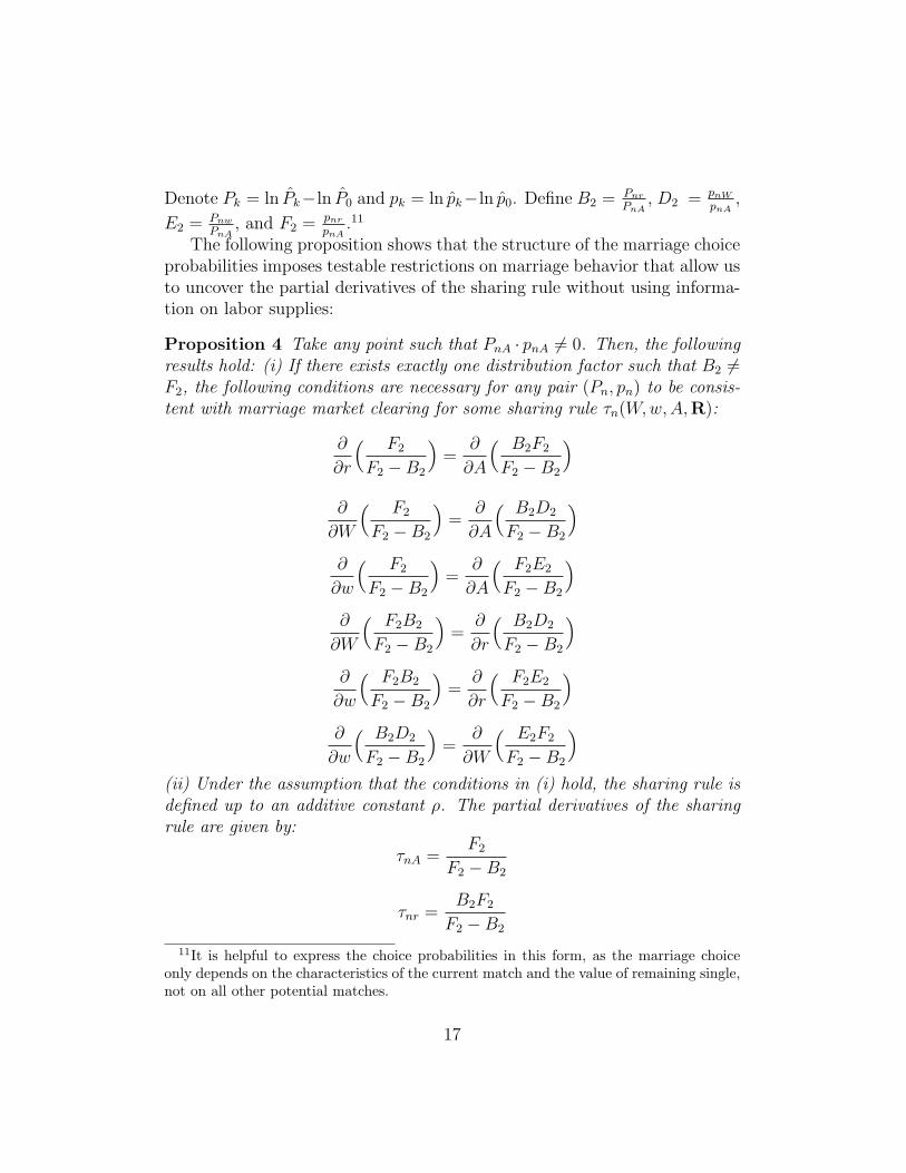
Proposition 4 Take any point such that PnA · pnA 6= 0. Then, the followingresults hold: (i) If there exists exactly one distribution factor such that B2 6=F2, the following conditions are necessary for any pair (Pn, pn) to be consis-tent with marriage market clearing for some sharing rule τn(W,w, A,R):

∂

∂r

( F2

F2 −B2

)=

∂

∂A

( B2F2

F2 −B2

)

∂

∂W

( F2

F2 −B2

)=

∂

∂A

( B2D2

F2 −B2

)

∂

∂w

( F2

F2 −B2

)=

∂

∂A

( F2E2

F2 −B2

)

∂

∂W

( F2B2

F2 −B2

)=

∂

∂r

( B2D2

F2 −B2

)

∂

∂w

( F2B2

F2 −B2

)=

∂

∂r

( F2E2

F2 −B2

)

∂

∂w

( B2D2

F2 −B2

)=

∂

∂W

( E2F2

F2 −B2

)

(ii) Under the assumption that the conditions in (i) hold, the sharing rule isdefined up to an additive constant ρ. The partial derivatives of the sharingrule are given by:

τnA =F2

F2 −B2

τnr =B2F2

F2 −B2

11It is helpful to express the choice probabilities in this form, as the marriage choiceonly depends on the characteristics of the current match and the value of remaining single,not on all other potential matches.

17

τnW =B2D2

F2 −B2

τnw =E2F2

F2 −B2

Proof: See Appendix C.1.12 Thus, information on marriage decisions allowsus to identify the partial derivatives of the sharing rule independently of thepartial derivatives identified from labor supplies. This provides us with thefollowing set of over-identifying restrictions

τnA =D1

D1 − F1

=F2

F2 −B2

τnr =D1F1

D1 − F1

=B2F2

F2 −B2

τnW =B1F1

D1 − F1

=B2D2

F2 −B2

(IN)

τnw =D1E1

D1 − F1

=E2F2

F2 −B2

that allow us to test whether the sharing rule that is consistent with familylabor supplies is a market clearing transfer.

12From the marriage decisions of the husband and wife, it is also straightforward toshow that we can uncover the partial derivatives of the indirect utilities:

qny = −(PnApnr − PnrpnA

Pnr

)

QnY =PnApnr − PnrpnA

pnr

QnW = PnW − PnrpnW

pnr

qnw = pnw − Pnwpnr

Pnr

18

5.2 Specialized couples

5.2.1 Labor supply

Consider couples in which only the husband works in the labor market. TheMarshallian labor supply function for husbands in specialized marriages is:

hs(w, A,R) = hs(w,A− τs(w, A,R)).

Denote non-labor incomes for the wife and husband, respectively, as:

Ys = τs(w,A,R)

ys = A− τs(w,A,R)

The partial derivatives of the labor supply function are

hsw = hsw − hsyτsw

hsA = hsy(1− τsA)

hsr = −hsyτsr

The above system has three equations and five unknowns. It is clear that ifwe only observe variation in the husband’s labor supply it is not possible touncover preferences and the sharing rule.

5.2.2 Marriage

The indirect utilities for wives and husbands in specialized marriages are:

Vs[εsG] = Qs[τs(w, A,R)] + Γs + εsG

vs[εsg] = qs[w,A− τs(w, A,R)] + γs + εsg

Denote the probability of choosing to be in a specialized marriage Ps forwomen and ps for men. The ratio of choice probabilities for specializedmarriage relative to remaining single is:

Ps

P0

=exp(Qs[τs(w, A,R)] + Γs)

exp(Q0[W0, Y0] + Γ0)

for women and

ps

p0

=exp(qs[w, A− τs(w, A,R)] + γs)

exp(q0[w0, y0] + γ0)

19

for men. As is the case for non-specialized marriages, the following propo-sition shows that it is straightforward to derive the partial derivatives ofthe sharing rule from marriage decisions. Define B3 = Psr

PsA, D3 = psr

psA, and

E3 = Psw

PsA. Then

Proposition 5 Take any point such that PnA · pnA 6= 0. Then, the followingresults hold: (i) If there exists exactly one distribution factor such that D3 6=B3, the following conditions are necessary for any pair (Ps, ps) to be consistentwith marriage market clearing for some sharing rule τs(w, A,R):

τsA =D3

D3 −B3

τsr =B3D3

D3 −B3

(IS)

τsw =D3E3

D3 −B3

Thus, it is possible to identify the sharing rule, up to an additive constant,for specialized couples if we observe changes in marriage behavior in responseto changes in wages, non-labor incomes, or market tightness.13 A conclusionthat immediately follows from the above is that it is always possible to iden-tify the sharing rule from marriage decisions in the absence of data on laborsupply.

6 Estimation and Model Tests

In this section, we outline our strategy for estimating and testing the collec-tive matching model. Our primary interest is in testing whether the sharingrule that clears the marriage market is consistent with the sharing rule thatrationalizes the labor supply decisions. Thus we are interested in testing therestrictions (IN) for nonspecialized couples.

We start by describing the data used to estimate our model. We nextdescribe our estimation strategy and and how we deal with special estimationissues raised by our data.

13As is the case for non-specialized couples, the indirect utilities and the sharing rules canboth be identified up to an additive constant. Once the partial derivatives of the sharingrule are known, it is straightforward to recover the partial derivatives of the Marshallianlabor supply function for husbands hy and hw.

20

6.1 Data

We use data from the 2000 US Census to estimate our model. For the pur-poses of our empirical analysis, we allow for the presence of many segregatedmarriage markets and many discrete types of men and women, where i de-notes the male’s type and j the female’s types. The type of each individual isdefined by the combination of race, education, and age. There are four racecategories (black, white, hispanic, other), and three education types (lessthan high school, high school graduate and/or some college, college gradu-ate). As a starting point, we consider individuals aged 21 to 60, grouped intofive year age categories (six age categories). There are 72 potential types ofwomen and men in the marriage market. As in CFL, we further assume thateach state constitutes a separate marriage market r, where marriage marketsare defined at the state level. Our unit of observation is (ijr) and there area total of 259, 200 possible cells.

Our goal is to test the over-identifying restrictions implied by the collec-tive matching model for nonspecialized couples. To this end, we limit oursample to couples in which both spouses work strictly positive hours. Wealso restrict our sample to couples without children. Our measure of laborsupply is annual hours of work. Wages are measured by average hourly earn-ings, constructed by dividing total labor income by annual hours. Nonlaborincome is measured as the sum several income sources including social secu-rity income, supplementary security income, welfare, interest, dividend andrental income, and other income. Wages, hours of work and nonlabor incomeare subsequently aggregated up to the cell level using the household samplingweights.14

The marital choice for women is defined as the log of the ratio of thenumber ijr marriages to the number of jr single women and likewise for men.Finally, market tightness for cell ijr is defined as the ratio of single men oftype i divided by single women of type j in market r. Many types of matches,for example across ethnic or education categories are relatively uncommon.We eliminate cells with less than five observations and observations for whomnonlabor income is negative. Finally we trim the top and bottom 3% of thewage, nonlabor income and sex ratio distributions to eliminate outliers. Ourfinal sample is contains ∗ cells.

Table 1 contains descriptive statistics for our sample of households. On

14Note that measurement error in earnings and hours at the individual level is reducedwhen the data are aggregated up to the cell level.

21

average, married men work more hours per year than married women, andmen have higher wages. The average level of nonlabor income in the sampleis slightly over $9, 000 and approximately 70% of households have children.The value for market tightness suggests that there is a slight shortage ofsingle men: there are 98 single men for every 100 single women.

Statistics on the ethnic, education, and age composition of marriages arepresented inTables 2, 3, and 4, respectively. As is well known from previousstudies, the vast majority of marriages (99%) are between men and womenof the same race, with marriages between white men and white women com-prising 90% of all marriages. With respect to other characteristics, individ-uals are also very likely to match within own-education categories (74% ofmarriages) and and own-age group (52% of marriages) but not to the sameextent as for race, especially regarding age as women are more likely to marryslightly older spouses.

6.2 Econometric Specification

Our primary interest is in testing whether the sharing rule that clears themarriage market is consistent with the sharing rule that rationalizes the la-bor supply decisions. Our tests of the collective matching model do not relyupon any particular functional form for preferences, thus it is desirable toimpose as few parametric assumptions on preferences as possible in our em-pirical analysis. The goal of this section is to outline a strategy for obtainingnonparametric estimates of our collective matching model. The reduced formlabor supply and marriage equations of interest are:

Hrij(W

rij, w

rij, A

rij,R

rij) = Hij[W

rij, τij(W

rij, w

rij, A

rij,R

rij)] (17)

hrij(W

rij, w

rij, A

rij,R

rij) = hij[w

rij, A

rij − τij(W

rij, w

rij, A

rij,R

rij)] (18)

and

P rij(W

rij, w

rij, A

rij,R

rij) = Pij[W

rij, τij(W

rij, w

rij, A

rij,R

rij), W

r0j, A

r0j] (19)

prij(W

rij, w

rij, A

rij,R

rij) = pij[w

rij, A

rij − τij(W

rij, w

rij, A

rij,R

rij), w

ri0, A

ri0] (20)

respectively. The vector Rrij is a vector of distribution factors that includes

the match specific sex ratio Srij and the wages and other incomes of single

men wri0, A

ri0 and wages and other incomes of single women W r

0j, Ar0j of the

22

same type as each spouse. Thus Rrij = {Sr

ij, wri0,W

r0j, A

ri0, A

r0j}.15

We introduce subscripts for the match type (ij) and the state of residencer to make two points. The first is that our framework (and our empiricalanalysis) is general enough to accommodate heterogeneity in preferences andsharing rules by match type. The second point is that an important iden-tifying assumption that preferences and invariant net gains can vary acrossdifferent types of matches, but not across locations. Thus, the partial deriva-tives of the labor supplies, the marriage log odds ratios (and therefore thesharing rules) will be identified off cross-state variation in hours worked andmarriage rates within match type. Estimation entails two stages:

Stage 1: Obtain nonparametric estimates of the partial derivatives ofthe reduced form labor supply (Hnx, hnx) and marriage matching equations(Pnx, pnx).

We estimate a semiparametric partially linear version of the model:

Hrij(W

rij, w

rij, A

rij,R

rij) = H[W r

ij, τij(Wrij, w

rij, A

rij,R

rij)] + αH

ij + eHrij (21)

hrij(W

rij, w

rij, A

rij,R

rij) = h[wr

ij, Arij − τij(W

rij, w

rij, A

rij,R

rij)] + αh

ij + ehrij (22)

and

P rij(W

rij, w

rij, A

rij,R

rij) = P [W r

ij, τij(Wrij, w

rij, A

rij,R

rij),W

r0j, A

r0j] + αP

ij + ePrij

prij(W

rij, w

rij, A

rij,R

rij) = p[wr

ij, Arij − τij(W

rij, w

rij, A

rij,R

rij), w

ri0, A

ri0] + αp

ij + eprij .

Our econometric specification differs from the most general version of ourmodel in two respects. First, we restrict the match type ij so that it onlyaffects the labor supplies and marriage log odds ratio through an intercept.This allows differences in match-specific characteristics to affect individuallabor supply and marriage market decisions, albeit in a limited way. Sec-ond, we introduce iid cell-specific error terms (eHr

ij , ehrij , ePr

ij , eprij ) that are

independent of wages, other incomes, and the sex ratio.

15We experimented with several alternative specifications, including a specification witha set of sex ratios that proxy an individual’s close substitutes in marriage: the ratio of menof the same age and race as the husband to women of the same age and race as the wifefor an ij couple of type, the ratio of men of the same age and education as the husbandto women of the same age and education as the wife, and the ratio of men of the samerace and education of the husband to women of the same race and education as the wife.The results for this specification can be found in Appendix D.2. The results from otherspecifications are available from the authors upon request.

23

We estimate the model using a combination of Robinson (1988) andSpeckman (1988) estimator and local linear estimation (Ruppert and Wand,1994). We illustrate our estimation procedure with the female labor supplyequation.16

Stage 2: Construct nonparametric estimates of the partial derivatives ofthe sharing rule from the first stage estimates and test the equality of themodel restrictions.

Recall, the test of the collective model we are interested in examiningis a test of the restrictions (IN), a test of whether the sharing rule thatis consistent with market clearing is also consistent with household laborsupplies. The set of restrictions we intend to test are

τnA =hnSHnA

hnSHnA −HnShnA

=pnSPnA

pnSPnA − PnSpnA

τnS =hnSHnS

hnSHnA −HnShnA

=pnSPnS

pnSPnA − PnSpnA

τnW =hnW HnS

hnSHnA −HnShnA

=pnW PnS

pnSPnA − PnSpnA

τnw =hnSHnw

hnSHnA −HnShnA

=pnSPnw

pnSPnA − PnSpnA

τnw0 =hnSHnw0

hnSHnA −HnShnA

=pnSPnw0

pnSPnA − PnSpnA

τnW0 =HnShnW0

hnSHnA −HnShnA

=pnW0PnS

pnSPnA − PnSpnA

τnAi0=

hnSHnAi0

hnSHnA −HnShnA

=pnSPnAi0

pnSPnA − PnSpnA

τnA0j=

HnShnA0j

hnSHnA −HnShnA

=pnA0j

PnS

pnSPnA − PnSpnA

16See Racine and Li (2007) for a full description of both methods and Appendix ?? fora full description of estimation for our particular model.

24

Step 1: Take the conditional expectation of Hn with respect to the non-parametric part of the model. Let s denote a vector containing W,w, A, T .Then

E[Hn|s] = E[X|s]′βH + Hn(s) (23)

and we difference from the labor supply equation to obtain:

Hn − E[Hn|s] = [X− E[X|s]]′βH + νH . (24)

Step 2: Estimate E[Hn|s] and E[X|s] by local linear regression. The locallinear estimator of the conditional mean function at s = (W,w, A, T ) is αand the derivative at this point is ρ. The local linear estimator for E[Hn|s]is:

minα,ρ

∑i

{Hni − α− ρ′(Si − s)

}24∏

h=1

K(Sih − sh

bh

)(25)

where K(·) is a one-dimensional kernel function, the bandwidth for the ith

covariate is bi and the kernel weight function is a product kernel. Fromstandard weighted least squares theory, the local linear estimator for theconditional mean is

Hn(s) = e1(S′sWsSs)

−1S′sWsHn (26)

where e1 is a 5 + 1 vector with 1 for the first element and 0 everywhere else,Hn = (Hn1, Hn2, ...HnN)′ where N is the number of observations,

Ws = diag{ 4∏

i=1

K(Si1 − si1

bi

). . .

4∏i=1

K(SiN − siN

bi

)}(27)

and

Ss =

1 (S1 − s)′...

...1 (SN − s)′

(28)

To get an estimate of the derivative of Hn(S) wrt to the k−th derivative,

ˆ∂Hn(s)

∂sk

= ek+1

(S′sWsSs

)−1X′

sWsHn (29)

25

Currently the i−th covariate bandwidth is set according to a rule of thumbof cσi/n

d+4 where σi is the standard deviation of the i−th covariate and nis the sample size. Refer to Ruppert and Wand (1994) for expressions of thebias and variance on the derivative estimate.

Step 3: Estimate

Hn − E[Hn|s] = [X− E[X|s]]′βH + νH .

using OLS to obtain βH .

Step 4: We can obtain an estimate of Hn(W,w, A, T ) as

Hn(W,w,A, T ) = E[Hn|s]− E[X|s]′βH (30)

7 Results

Coming soon.The actual values of the parameter estimates for the sharing rule are in

Appendix D.1.

8 Conclusion

In this paper, we develop and estimate an empirical collective matchingmodel. Our model integrating the collective model of Chiappori (1992) andthe matching model of Choo and Siow (2006). We establish that two modelsfit together without modification and can be analyzed independently, as donein previous studies. The sharing rule in our collective matching model arisesendogenously as a transfer that clears the marriage market. In addition tomarital matching between different types of individuals, the model can in-corporate participation decisions of one or both spouses. With informationon at least two independent marriage markets, incorporating matching in thecollective model allows us to identify the sharing rule from observations onmarriage decisions, regardless of the labor supply decisions of wives and hus-bands. Introducing the marriage market in the collective model generatesover-identifying restrictions that allow us to test whether the sharing rulethat rationalizes labor supplies is consistent with the sharing rule that clearsthe marriage market.

26

Table 1: Household Characteristics

Husbands Wives

Annual hours 2262.16 1726.86Average hourly wage 25.11 17.61Nonlabor income 9,333.18

Fraction of households with children 0.69Market tightness 0.69

Cells 13,990

27

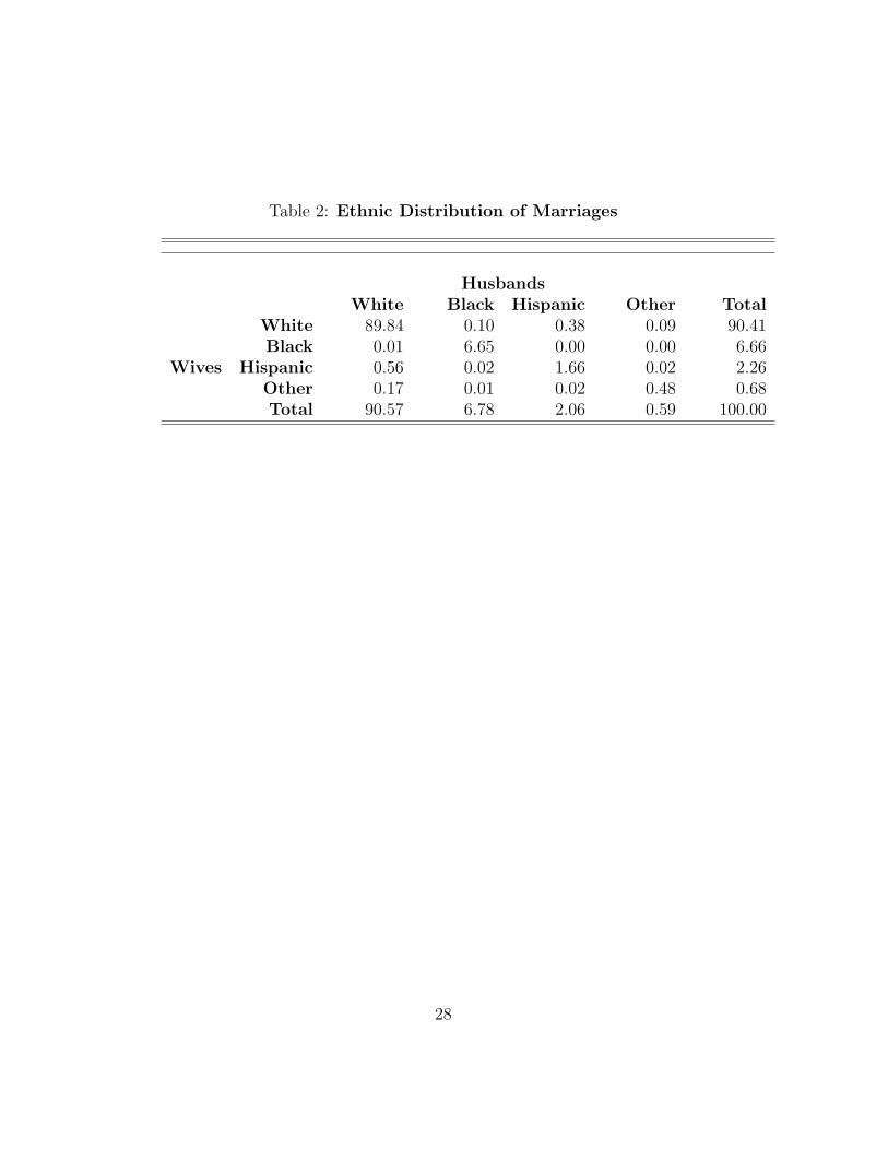
Table 2: Ethnic Distribution of Marriages

HusbandsWhite Black Hispanic Other Total

White 89.84 0.10 0.38 0.09 90.41Black 0.01 6.65 0.00 0.00 6.66

Wives Hispanic 0.56 0.02 1.66 0.02 2.26Other 0.17 0.01 0.02 0.48 0.68Total 90.57 6.78 2.06 0.59 100.00

28

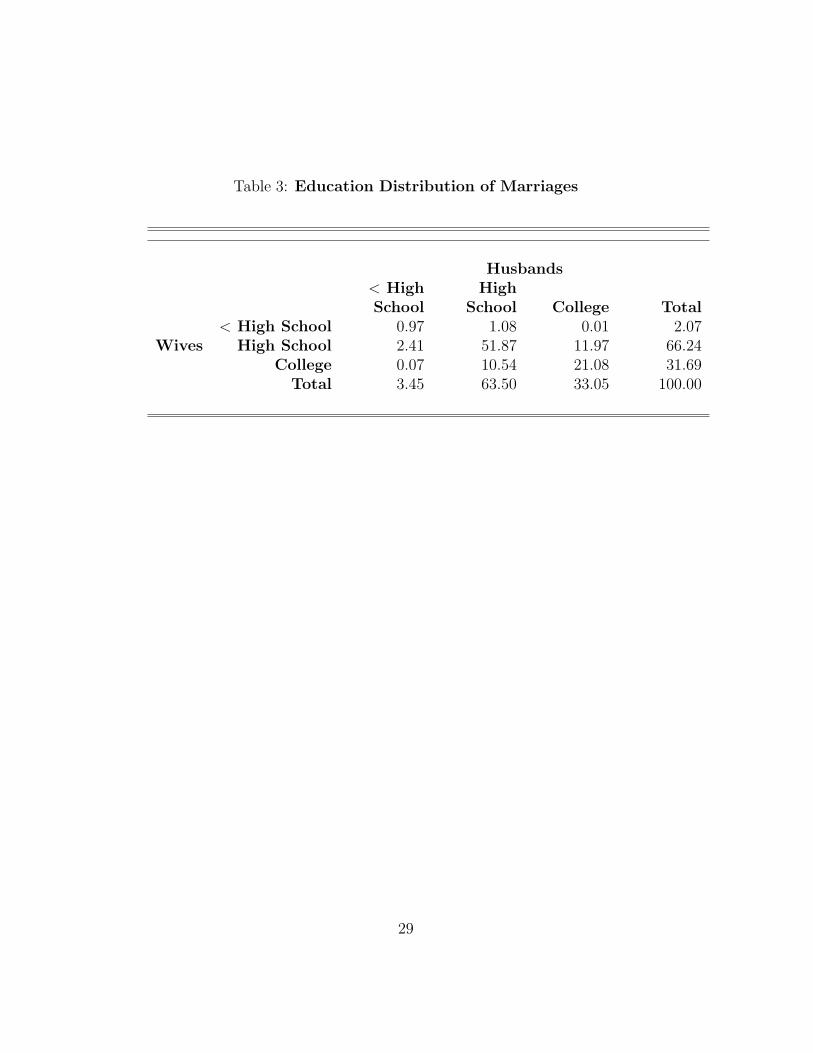
Table 3: Education Distribution of Marriages

Husbands< High HighSchool School College Total

< High School 0.97 1.08 0.01 2.07Wives High School 2.41 51.87 11.97 66.24

College 0.07 10.54 21.08 31.69Total 3.45 63.50 33.05 100.00

29

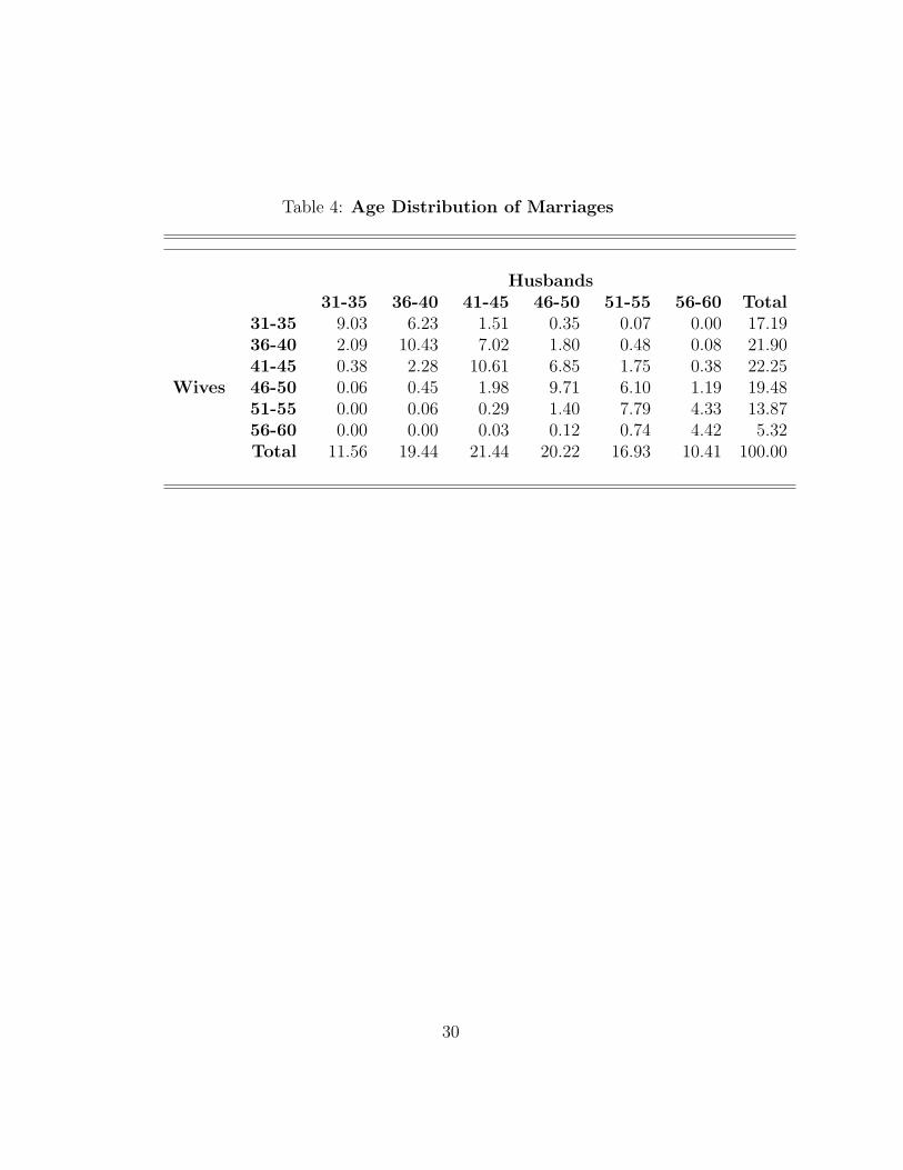
Table 4: Age Distribution of Marriages

Husbands31-35 36-40 41-45 46-50 51-55 56-60 Total

31-35 9.03 6.23 1.51 0.35 0.07 0.00 17.1936-40 2.09 10.43 7.02 1.80 0.48 0.08 21.9041-45 0.38 2.28 10.61 6.85 1.75 0.38 22.25

Wives 46-50 0.06 0.45 1.98 9.71 6.10 1.19 19.4851-55 0.00 0.06 0.29 1.40 7.79 4.33 13.8756-60 0.00 0.00 0.03 0.12 0.74 4.42 5.32Total 11.56 19.44 21.44 20.22 16.93 10.41 100.00

30

Tab

le5:

Sem

i-para

metr

icla

bor

supply

est

imate

s

Wiv

esH

usb

ands

Age

s21

-60

Age

s21

-30

<co

lleg

eA

ges

21-6

0A

ges

21-3

0<

colleg

e

Oth

erin

com

e-4

.908

1-3

1.10

07-6

0.03

77-3

.652

3-1

6.03

76-5

3.78

31Sex

rati

o25

.388

6-2

7.05

5512

5.55

432.

2124

33.2

901

155.

8961

Husb

and’s

wag

e-7

3.82

2639

5.19

50-9

82.1

317

-368

.923

9-4

85.0

592

-212

2.36

11W

ife’

sw

age

20.2

379

519.

6946

2284

.038

558

.721

832

0.99

6820

64.8

422

Sin

gle

mal

ew

age

96.5

217

364.

5089

1727

.752

413

4.80

0910

65.5

490

4085

.049

2Sin

gle

mal

ein

com

e12

.388

120

.751

2-6

7.49

78-7

.973

3-2

8.48

73-9

2.57

67Sin

gle

fem

ale

wag

e57

4.42

6556

7.79

8312

10.4

147

-230

.455

467

8.66

4511

8.71

58Sin

gle

fem

ale

inco

me

-15.

8679

-72.

2159

-159

.879

20.

2793

-38.

1971

-282

.350

5

Obse

rvat

ions

5206

666

261

5206

666

261

31

Tab

le6:

Sem

i-para

metr

icm

arr

iage

log

odds

est

imate

s

Wiv

esH

usb

ands

Age

s21

-60

Age

s21

-30

<co

lleg

eA

ges

21-6

0A

ges

21-3

0<

colleg

e

Oth

erin

com

e0.

1630

0.22

590.

2126

0.16

330.

2051

0.21

12Sex

rati

o1.

0165

0.33

300.

3087

-0.2

750

-0.5

060

-0.5

265

Husb

and’s

wag

e3.

7942

0.37

791.

4482

3.66

350.

7458

1.44

47W

ife’

sw

age

1.08

94-0

.107

4-5

.715

10.

8258

-0.4

208

-5.7

086

Sin

gle

mal

ew

age

-6.4

758

-13.

1600

-24.

1142

-7.2

044

-13.

1300

-19.

5708

Sin

gle

mal

ein

com

e-0

.066

5-0

.188

6-0

.411

7-0

.073

3-0

.134

4-0

.371

5Sin

gle

fem

ale

wag

e-7

.104

8-1

1.20

79-9

.808

5-6

.465

2-1

0.76

14-1

1.23

77Sin

gle

fem

ale

inco

me

-0.1

306

-0.4

795

-0.1

153

-0.1

203

-0.4

510

-0.0

112

Obse

rvat

ions

5206

666

261

5206

666

261

32

Tab

le7:

Change

inτ

wit

hre

spect

toa

10%

incr

ease

invari

able

(as

aperc

enta

ge

ofoth

er

inco

me

inpare

nth

ese

s)

Lab

orSupply

Mar

riag

e

Age

s21

-60

Age

s21

-30

<co

lleg

eA

ges

21-6

0A

ges

21-3

0<

colleg

e

Oth

erin

com

e78

.49

43.9

933

.24

63.7

146

.42

29.7

5[3

.38]

[5.5

0][6

.83]

[5.8

0][2

.75]

[6.1

1]Sex

rati

o-2

2.86

5.97

-25.

261.

561.

1621

.57

[-0.

99]

[0.7

5][-5.

19]

[0.1

5][0

.07]

[4.4

3]H

usb

and’s

wag

e-3

1.85

-12.

5746

.25

126.

95-1

00.1

310

7.19

[-1.

37]

[-1.

57]

[9.5

0][-12

.52]

[5.4

7][2

2.02

]W

ife’

sw

age

-54.

7947

.91

-130

.32

8.13

28.7

164

.69

[-2.

36]

[5.9

9][-26

.78]

[3.5

9][0

.35]

[13.

29]

Sin

gle

mal

ew

age

81.0

5-4

6.82

-89.

09-9

1.24

-392

.45

-291

.60

[3.4

9][-5.

85]

[-18

.30]

[-49

.06]

[-3.

93]

[-59

.91]

Sin

gle

mal

ein

com

e-4

1.03

-20.

9935

.20

-32.

52-2

7.13

-17.

35[-1.

77]

[-2.

62]

[7.2

3][-3.

39]

[-1.

40]

[-3.

56]

Sin

gle

fem

ale

wag

e-1

43.3

018

.89

33.0

316

3.23

137.

0565

.30

[-6.

18]

[2.3

6][6

.79]

[17.

13]

[7.0

4][1

3.42

]Sin

gle

fem

ale

inco

me

1605

.90

-1.9

7-1

.16

2063

.52

723.

0832

7.35

[1.3

7][-0.

25]

[-0.

24]

[90.

39]

[88.

97]

[67.

35]

Obse

rvat

ions

5206

666

261

5206

666

261

33

References

[1] Becker, Gary (1973). “A Theory of Marriage: Part I,” Journal of Polit-ical Economy, 81(4), 813-46.

[2] Becker, Gary (1974). “A Theory of Marriage: Part II,” Journal of Po-litical Economy, 82(2), S11-S26, Part II.

[3] Becker, Gary (1991). A Treatise on the Family, Harvard UniversityPress, Second Edition.

[4] Becker, Gary and Kevin Murphy (2000). Social Economics. Cambridge,MA: Harvard University Press.

[5] Blundell, Richard, Browning, Martin, and Ian Crawford (2003). “Non-parametric Engel Curves and Revealed Preference,” Econometrica,71(1), 205-240.

[6] Blundell, Richard, Chiappori, Pierre-Andre, Magnac, Theirry, andCostas Meghir (2007). “Collective Labour Supply: Heterogeneity andNon-Participation,” Review of Economic Studies, 74(2), 417-445.

[7] Blundell, Richard, Chiappori, Pierre-Andre, and Costas Meghir (2006).“Collective Labor Supply with Children,” Journal of Political Economy,113(6), 1277-1306.

[8] Brien, Michael (1997). “Racial Differences in Marriage and the Role ofMarriage Markets,” Journal of Human Resources, 32(4), 741-778.

[9] Brien, Michael, Lillard, Lee, and Steven Stern (2006) “Cohabitation,Marriage, and Divorce in a Model of Match Quality,” International Eco-nomic Review, 47(2), 451-494.

[10] Browning, Martin and Pierre-Andre Chiappori (1998). “Efficient Intra-Household Allocations: A General Characterization and EmpiricalTests,” Econometrica, 66(6), 124-1278.

[11] Browning, Martin, Chiappori, Pierre-Andre, and Yoram Weiss (2003).“A Simple Matching Model of the Marriage Market,” University ofChicago, unpublished manuscript.

34

[12] Cherchye, Laurens, De Rock, Bram, and Frederick Vermeulen (2007).“The Collective Model of Household Consumption: A NonparametricCharacterization,” Econometrica, 75(2), 553-574.

[13] Chiappori, Pierre-Andre (1988). “Rational Household Labor Supply,”Econometrica 56(1), 63-90.

[14] Chiappori, Pierre-Andre (1992). “Collective Labor Supply and Welfare,”Journal of Political Economy, 100(3), 437-467.

[15] Chiappori, Pierre-Andre and Ivar Ekelund (2006). “The Micro Eco-nomics of Efficient Group Behavior: Identification,” Columbia Univer-sity working paper.

[16] Chiappori, Pierre-Andre, Fortin, Bernard, and Guy Lacroix (2002).“Household Labor Supply, Sharing Rule, and the Marriage Market,”Journal of Political Economy, 110(1), 37-72.

[17] Chiappori, Pierre-Andre, Iyigun, Murat, and Yoram Weiss (2006). “In-vestment Schooling and the Marriage Market,” IZA Working Paper No.2454, November.

[18] Choo, Eugene and Aloysius Siow (2005). “Lifecycle Marriage Matching:Theory and Evidence,” University of Toronto working paper.

[19] Choo, Eugene and Aloysius Siow (2006). “Who Marries Whom andWhy,” Journal of Political Economy, 114(1), 175-201.

[20] Del Boca, Daniela and Christopher Flinn (2006a) “Endogenous House-hold Interaction,” NYU working paper.

[21] Del Boca, Daniela and Christopher Flinn (2006b) “Household Time Al-location and Modes of Behavior: A Theory of Sorts,” NYU workingpaper.

[22] Duflo, Esther (2003). “Grandmothers and Granddaughters: Old AgePension and Intra-household Allocation in South Africa,” World BankEconomic Review, 17(1), 1-25.

[23] Fortin, Bernard and Guy Lacroix (1997). “A Test of the Unitary andCollective Models of Household Labour Supply,” Economic Journal,107(443), 933-955.

35

[24] Grossbard, Shoshana and Shoshana Grossbard and Catalina Amuedo-Dorantes (2007). “Cohort Level Sex Ratio Effects on Women’s LaborForce Participation,” Review of Economics of the Household, 5(3), 249-278.

[25] Grossbard-Schectman, Amyra (1984). “ A Theory of Allocation of Timein Markets for Labour and Marriage.” The Economic Journal 94(376),863-82.

[26] Grossbard-Schectman, Shoshana (1993). On the Economics of Marriage:A Theory of Marriage, Labor, and Divorce, Boulder, Colorado: West-view Press.

[27] Grossbard-Schectman, Shoshana and Clive Granger (1998). “WomensJobs and Marriage, Baby-Boom versus Baby-Bust,” Population, 53, 731-52, September 1998.

[28] Iyigun, Murat and Randall Walsh (2007). “Building the Family Nest:Premarital Investments, Marriage Markets, and Spousal Allocations,”Review of Economic Studies, 74(2), 507-535.

[29] Kelso Alexander and Vincent Crawford (1982). “Job Matching, Coali-tion Formation, and Gross Substitutes,” Econometrica, 50, 1483-1504.

[30] Li, Qi and Jeffrey Racine (2007). Nonparametric Econometrics, Prince-ton University Press.

[31] Lise, Jeremy and Shannon Seitz (2007). “Consumption Inequalityand Intra-Household Allocations,” Queen’s University, unpublishedmanuscript.

[32] Lundberg, Shelly (1988). “Labor Supply of Husbands and Wives: A Sim-ulataneous Equations Approach,” The Review of Economics and Statis-tics, 70(2), 224-235.

[33] Lundberg, Shelly, and Robert Pollak (1996). “Bargaining and Distribu-tion in Marriage,” Journal of Economic Perspectives, 10(4), 139-158.

[34] Manser, Marilyn, and Murray Brown (1980). “Marriage and HouseholdDecision-Making: A Bargaining Analysis.” International Economic Re-view, 21(1), 31-44.

36

[35] Mas-Colell, Andreu, Green, Jerry and Michael Whinston (1995). Mi-croeconomic Theory. Oxford University Press.

[36] Mazzocco, Maurizio (2004). “Saving, Risk Sharing and Preferences forRisk,” American Economic Review, 94(4), 1169-1182.

[37] Mazzocco, Maurizio, and Shintaro Yamaguchi (2006). “Labor Supply,Wealth Dynamics, and Marriage Decisions,” University of Wisconsin-Madison, unpublished manuscript.

[38] McElroy, Marjorie (1990). “The Empirical Content of Nash-BargainedHousehold Behavior,” The Journal of Human Resources, 25(4), 559-583.

[39] McElroy, Marjorie and Mary-Jean Horney (1981). “Nash-BargainedHousehold Decisions: Toward a Generalization of the Theory of De-mand.” International Economic Review, 22(2), 333-349.

[40] McFadden, Daniel (1974). “Conditional Logit Analysis of QualitativeChoice Behavior.” In Frontiers in Econometrics, edited by Paul Zarem-bka. New York: Academic Press.

[41] Robinson, P. (1988). “Root N-Consistent Semiparametric Regression,”Econometrica, 56, 931-954.

[42] Ruppert, D. and M. Wand (1994). “Multivariate Locally Weighted LeastSquares Regression,” The Annals of Statistics, 22(3), 1346-1370.

[43] Seitz, Shannon (2004). “Accounting for Racial Differences in Marriageand Employment,” Queen’s University working paper.

[44] Speckman, P. (1988) “Kernel Smoothing in Partial Linear Models,”Journal of the Royal Statistical Society, Series B, 50, 413-446.

[45] Thomas, Duncan (1990). “Intra-Household Resource Allocation: An In-ferential Approach,” The Journal of Human Resources, 25(4), 635-664.

[46] Vermeulen, Frederick (2006). “A Collective Model for Female LabourSupply with Nonparticipation and Taxation,” Journal of PopulationEconomics, 19(1), 99-118.

37

A Proof of Proposition 1

Abstracting from gG, the social planner solves:

max{C,c,H,h}

E(Q(C, 1−H, K|Z) + pE(q(c, 1− h,K)|Z)

subject to, for each state S,

c + C + K ≤ A + W (1−H) + w(1− h) (31)

Let Z∗ be the value of Z evaluated at the optimum. The first orderconditions with respect to c, C, H, h, K and the multiplier λ for each stateS are:

Q∗c = λ (32)

pq∗c = λ (33)

Q∗1−H = λW (34)

pq∗1−h = λw (35)

Q∗K + pq∗K = λ (36)

Using the first order conditions, as p changes, for each state S,

∂Q∗

p∂p=

λ

p(C∗

p + WL∗p + K∗p)− q∗KK∗

p (37)

∂q∗

∂p=

λ

p(c∗p + wl∗p) + q∗KK∗

p (38)

∂Q∗

p∂p+

∂q∗

∂p=

λ

p(c∗p + wl∗p + K∗

p + C∗p + WL∗p)) (39)

Since the budget constraint has to hold for every S,

c∗p + C∗p + K∗

p + wl∗p + WL∗p = 0

∂Q∗

∂p= −p

∂q∗

∂p(40)

Since (40) holds for every state S, (??) obtains.

38

B Proof of Existence of Equilibrium

In the proof, we need:

Eij(p) > 0 as p →∞ (Condition A1)

Eij(p) < 0 as p → 0 (Condition A2)

That is, the utility functions q and Q must be such that as p approaches0, men will not want to marry. And as p approaches ∞, women will not wantto marry.

Let βij = (1 + pij)−1 where βij ∈ [0, 1] is the utility weight of the wife in

an {i, j} marriage and (1− βij) is the utility weight of the husband.We know:

∂µij

∂pij

> 0 (41)

∂µij

∂pik

< 0, k 6= j (42)

∂µkl(β)

∂pij

= 0; k 6= i, l 6= j (43)

∂µij

∂pij

< 0 (44)

∂µij

∂pkj

> 0, k 6= i (45)

∂µkl(β)

∂pij

= 0; k 6= i, l 6= j (46)

Let β be a matrix with typical element βij and the IxJ matrix functionE(β) be:

E(β) = µ(β)− µ(β) (47)

An element of E(β), Eij(β), is the excess demand for j type wives by itype men given β.

An equilibrium exists if there is a β∗ such that E(β∗) = 0.Assume that there exists a function f(β) = αE(β)+β, α > 0 which maps

[0, 1]I∗J → [0, 1]I∗J and is non-decreasing in β. Tarsky’s fixed point theoremsays if a function f(β) maps [0, k]N → [0, k]N , k > 0, and is non-decreasingin β, there exists β∗ ∈ [0, k]N such that β∗ = f(β∗). Let f(β) = αE(β) + β,

39

k = 1 and N = I ∗J , and apply Tarsky’s theorem to get β∗ = αE(β∗)+β∗ ⇒E(β∗) = 0.

Thus the proof of existence reduces to showing f(β) which has the re-quired properties.

We know from (41) to (46) that:

∂Eij(β)

∂βij

< 0 (48)

∂Eik(β)

∂βij

> 0 (49)

∂Ekj(β)

∂βij

> 0 (50)

∂Ekl(β)

∂βij

= 0; k 6= i, l 6= j (51)

(48) to (51) imply that E(β) satisfies the Weak Gross Substitutability(WGS) assumption.

We now show that the WGS property of E(β) implies that we can con-struct f(β), such that f(β) maps [0, 1]I∗J → [0, 1]I∗J and is non-decreasing inβ. The proof follows the solution to exercise 17.F.16C of Mas-Colell, Whin-ston and Green given in their solution manual. (N.B. Unlike them, we donot start with Gross Substitution, we begin from WGS, but it turns out tobe sufficient for Tarsky’s conditions)

For notational convenience, now onwards we’ll treat the matrix functionE(β), as a vector function.

Let N = I ∗ J and 1N be a N × 1 vector of ones. E(β) : [0, 1]N → RN

is continuously differentiable and satisfies E(0N) >> 0N and E(1N) << 0N

(Conditions A1 and A2).For every β ∈ [0, 1]N and any n, if βn = 0, then En(β) > 0.For every β ∈ [0, 1]N and any n, if βn = 1, then En(β) < 0.If β = {0N , 1N}, the facts follow from Conditions A1 and A2. Otherwise,

they are due to Conditions A1 and A2, and (48) to (51), i.e. WGS.For each n, define Cn = {β ∈ [0, 1]N : En(β) ≥ 0} and Dn = {β ∈ [0, 1]N :

En(β) ≤ 0}.Then Cn ⊂ {β ∈ [0, 1]N : βn < 1} and Dn ⊂ {β ∈ [0, 1]N : βn > 0}.Then by continuity, the following two minima, ij((1−βn)/En(β) : β ∈ Cn)

and ij(−βn/En(β) : β ∈ Dn), exist and are positive. Let βn

> 0 be smaller

40

than those two minima. Then, for all α ∈ (0, βn) and any β ∈ [0, 1]N , we

have 0 ≤ αEn(β) + βn ≤ 1.For each n, define Ln =ij {|∂En(β)/∂βn| : β ∈ [0, 1]N}. Then, for all

α ∈ (0, 1/Ln),

∂(αEn(β) + βn)

∂βn

= α∂En(β)

∂βn

+ 1 ≥ −αLn + 1 > 0

∂(αEn(β) + βn)

∂βm

= α∂En(β)

∂βm

≥ 0; n 6= m, follows from (48) to (51).

Now let K = ij{β1, .., β

N, 1/L1, .., 1/LN}, choose α ∈ (0, K), then f(β) =

αE(β) + β ∈ [0, 1]N and ∂f(β)/∂βn ≥ 0 for every β ∈ [0, 1]N , and any n.Hence Tarsky’s conditions are satisfied.

C Identification

C.1 Marriage, non-specialized couples

Denote the probability of choosing to be in a non-specialized marriage Pn

and the probability of being single P0, respectively for women and pn and p0

for men. Under the extreme value assumption for we can express the ratioof the choice probabilities for non-specialized marriage relative to remainingsingle as:

Pn

P0

=exp(Qn[W,Yn] + Γn)

exp(Q0[W0, Y0] + Γ0)

for women andpn

p0

=exp(qn[w, yn] + γn)

exp(q0[w0, y0] + γ0)

Denote Pn = ln Pn − ln P0 and pn = ln pn − ln p0.Differentiating with respect to wages, household non-labor income and µ

41

yields:

PnA = QnY τnA

PnT = QnY τnT

PnW = QnW + QnY τnW

Pnw = QnY τnw

for women and

pnA = qny(1− τnA)

pnT = −qnyτnT

pnw = qnw − qnyτnw

pnW = −qnyτnW

C.2 Marriage, specialized couples

Denote the probability of choosing to be in a specialized marriage Ps andthe probability of being single P0, respectively for women and ps and p0 formen. Under the extreme value assumption for we can express the ratio ofthe choice probabilities for specialized marriage relative to remaining singleas:

Ps

P0

=exp(Qs[Ys] + Γs)

exp(Q0[W0, Y0] + Γ0)

for women andps

p0

=exp(qs[w, ys] + γs)

exp(q0[w0, y0] + γ0)

D Additional estimation results

D.1 Parameter estimates for sharing rule

42

Tab

le8:

Shari

ng

rule

est

imate

sand

test

stati

stic

s

Ben

chm

ark

Age

s21

-30

<co

lleg

e

Lab

orsu

pply

Mar

riag

eLab

orsu

pply

Mar

riag

eLab

orsu

pply

Mar

riag

e

Oth

erin

com

e0.

3384

0.28

470.

5499

0.58

020.

6829

0.61

12Sex

rati

o-0

.310

90.

0212

0.05

850.

0114

-0.2

549

0.21

77H

usb

and’s

wag

e-1

.808

87.

2092

-0.9

678

-7.7

086

4.04

989.

3865

Wife’

sw

age

-4.3

555

0.64

574.

3597

2.61

23-1

4.13

487.

0168

Sin

gle

mal

ew

age

5.20

56-5

.860

1-3

.950

9-3

3.11

78-8

.624

3-2

8.22

82Sin

gle

mal

ein

com

e-0

.271

9-0

.215

5-0

.373

0-0

.482

10.

9540

-0.4

702

Sin

gle

fem

ale

wag

e-1

1.17

7712

.732

71.

8344

13.3

063

3.85

867.

6280

Sin

gle

fem

ale

inco

me

0.19

7812

.849

6-0

.033

912

.449

8-0

.021

15.

9870

Obse

rvat

ions

5206

666

261

5206

666

261

43

D.2 Estimation results for specification where the shar-ing rule includes measures of close substitutes.

44

Tab

le9:

Sem

i-para

metr

icla

bor

supply

est

imate

s

Wiv

esH

usb

ands

Ben

chm

ark

Age

s21

-30

<co

lleg

eB

ench

mar

kA

ges

21-3

0<

colleg

e

Oth

erin

com

e19

.335

715

.538

66Sex

rati

o-7

5.60

33-1

99.8

190

Husb

and’s

wag

e13

03.4

035

-122

9.56

91W

ife’

sw

age

181.

0737

-372

.742

5Sin

gle

mal

ew

age

-771

.194

5-2

08.8

846

Sin

gle

mal

ein

com

e43

7.74

2432

2.24

68Sin

gle

fem

ale

wag

e-2

7.41

1327

4.28

10Sin

gle

fem

ale

inco

me

2561

.496

414

05.4

254

Sex

rati

oby

age

and

race

71.6

046

-22.

7786

Sex

rati

oby

age

and

educa

tion

195.

0148

1104

.422

6Sex

rati

oby

race

and

educa

tion

-3.9

183

-366

.025

7

Obse

rvat

ions

5206

666

5206

666

45

Tab

le10

:Sem

i-para

metr

icm

arr

iage

log

odds

est

imate

s

Wiv

esH

usb

ands

Ben

chm

ark

Age

s21

-30

<co

lleg

eB

ench

mar

kA

ges

21-3

0<

colleg

e

Oth

erin

com

e0.

1685

0.06

89Sex

rati

o1.

4213

0.34

50H

usb

and’s

wag

e4.

4192

0.66

24W

ife’

sw

age

0.97

485.

3799

Sin

gle

mal

ew

age

-0.7

691

1.02

38Sin

gle

mal

ein

com

e0.

3656

-0.6

740

Sin

gle

fem

ale

wag

e0.

9292

0.41

77Sin

gle

fem

ale

inco

me

-1.3

677

-18.

1905

Sex

rati

oby

age

and

race

-0.2

247

-0.3

793

Sex

rati

oby

age

and

educa

tion

-13.

7379

1.99

99Sex

rati

oby

race

and

educa

tion

-0.0

255

0.10

17

Obse

rvat

ions

5206

666

5206

666

46

Tab

le11

:Shari

ng

rule

est

imate

sand

test

stati

stic

s

Ben

chm

ark

Age

s21

-30

<co

lleg

e

Lab

orsu

pply

Mar

riag

eLab

orsu

pply

Mar

riag

eLab

orsu

pply

Mar

riag

e

Oth

erin

com

e0.

4114

0.08

90Sex

rati

o-0

.287

10.

2153

Husb

and’s

wag

e3.

9071

3.07

25W

ife’

sw

age

-3.9

949

0.35

63Sin

gle

mal

ew

age

-0.0

444

-0.5

383

Sin

gle

mal

ein

com

e-0

.864

9-7

.872

8Sin

gle

fem

ale

wag

e-0

.006

90.

4244

Sin

gle

fem

ale

inco

me

-0.0

186

-0.4

522

Sex

rati

oby

age

and

race

-0.0

599

-0.4

137

Sex

rati

oby

age

and

educa

tion

-1.0

051

0.22

33Sex

rati

oby

race

and

educa

tion

-3.3

346

-0.2

906

Obse

rvat

ions

5206

666

5206

666

47