Leila Al-Mqbali

5600405

65

An Empirical Investigation of the Random Walk

Hypothesis in the US and UK Stock Markets

Do Well Developed Economies with High Market Capitalization Yield the Same Conclusions?

Leila Al-Mqbali Student Number: 5600405

Major Paper submitted to the University of

Ottawa Department of Economics, in order to

complete the requirements of the MA

Economics degree.

Supervisor: Professor FrancescaRondina ECO6999

Ottawa, Ontario August 2015

[Type a quote from the document or the summary of an interesting point. You can position the text box

anywhere in the document. Use the Text Box Tools tab to change the formatting of the pull quote text

box.]

Leila Al-Mqbali

5600405

i

Abstract

This paper assesses the validity of random walk in the US and UK stock markets, in order to

assess whether controlling for the size of market capital and the extent of economic development

impacts results. We find that results are not robust to the empirical techniques employed, nor are

they robust to the choice of horizon length. Therefore, the lack of consensus in professional

opinion regarding the validity of the random walk hypothesis cannot be wholly attributed to

differences in market capital and economic development. Future research should attempt to

control for other factors such as trading frequency and volume, with the aim of identifying key

economic dynamics which influence the results.

Leila Al-Mqbali

5600405

1

I. Introduction

In recent years, there has been increased interest in the behaviour of stock market returns,

and as yet there is no clear consensus among experts with regards to their predictability. This

paper will assess whether stock prices in the US and UK markets tend to follow a random walk.

The random walk hypothesis (RWH) relies on two premises: (1) stock price changes

conform to some probability distribution, and (2) stock price changes are independent of each

other, which implies that previous movements in stock prices cannot be used to forecast future

changes. Investors react instantaneously to any new information they are presented with, and this

competition between investors eliminates all prospects of profiting from such information.

Advocates of RWH thus maintain that stocks take an unpredictable and random path, and as a

consequence it is impossible to outperform the market as stock prices reflect all information

available at the time of exchange. Conversely, opponents of RWH argue that stock price changes

are, at least to some extent, predictable.

Previous results from testing the validity of RWH appear to be sensitive to the empirical

tests conducted as well as the particular market which is studied. However, as yet, research has

focusedon using a variety of empirical methods to assess RWH in a particular country, rather

than exploring how their results may differ across countries when each index is subjected to the

same empirical methods. This project will therefore determine whether stock indices in two

markets which are very similar in terms of size of market capital and the extent of economic

development yield the same conclusions when subjected to the same empirical tests for RWH.

More specifically, we will focus on the UK and US economies, two well developed

markets with high market capitalization.Our empirical methods include a subset of various

parametric and non-parametric tests frequently employedby researchers testing for RWH. If our

results differ between indices, then we must acknowledge that the difference must be due not

todissimilarities in market capitalization and economic development, but rather to some

unknown market characteristic which has not been accounted for. If, on the other hand, we

obtain similar results for each index, then future research can attempt to extend this analysis to

Leila Al-Mqbali

5600405

2

demonstrate that, in general, well developed markets with high market capitalization will yield

the same conclusions with regards to RWH.

This research will be a valuable contributor to the existing literature on the RWH in several

ways. First, no previous papers have focussed on a comparative analysis of the RWH for indices

in two well developed countries with similar market characteristics using such an extensive array

of empirical methods. Second, Section V of this paper presents a thorough and comprehensive

description of the primary parametric and non-parametric tests used to assess the validity of

RWH, which researchers may find to be a useful reference for future studies in this area.

The next section will present a review of previous literature on the RWH.Early theoretical

contributions in this area were followed by empirical studies that addressed the behaviour of

stock market returns through a variety of empirical techniques. As we will see, these studies

provide evidence both for and against RWH, as results appear to be sensitive to the tests

employed as well as the market which is studied.

II. A Review of Previous Literature

An Early Theoretical Argument for RWH

The doctoral thesis of French mathematician Louis Bachelier(2006, originally published in

1900) documents an early discussion of the random walk hypothesis in financial markets. In

Théorie de la Spéculation, Bachelier investigates the market for French government bonds and

notes that “the influences that determine the movements of the exchange are innumerable; past,

current and even anticipated events that often have no obvious connection with its changes ... it

is thus impossible to hope for mathematical predictability” (Bachelier, 2006, p. 15).

Consequently, Bachelier infers a fundamental hypothesis that predates much of the existing

literature on RWH: since it is not possible to predict future movements in the market, the

mathematical expectation of the economic agent is equivalent to zero (p. 18).

However, Bachelier’s work did not receive widespread notice outside the field of

mathematics until the 1950s, when economist Paul Samuelson connected the theory of random

Leila Al-Mqbali

5600405

3

walk in stock markets with economic fundamentals. Samuelson (1965) proposes a theoretical

argument that the market achieves randomness through the competitive activities of a large

number of investors all seeking to increase their wealth. Creating a general stochastic model of

price change, he demonstrates that the price differences in any one period are uncorrelated with

the price differences in the previous period; in other words, there is zero expected capital gain.

However, Samuelson did emphasize that his theory does not suggest that it would be impossible

for one investor who has superior information to make a profit – only that it is unlikely they can

outperform the market average. Throughout his career, Samuelson continued to propose

theoretical frameworks in support of RWH; yet he did not conduct econometric and empirical

research to test his hypotheses. The following section will address empirical findings on the

subject.

Empirical Evidence

Following Samuelson’s research, Fama (1965) found that there was strong evidence to

support RWH. Using daily stock prices as data, Fama employed statistical techniques to show

both the independence of stock price movements and their conformity to stable Paretian

distributions with characteristic exponents less than 2. Moreover, Osborne (1959) supports

Fama’s results. Using the theory of Brownian motion applied to financial markets, Osborne

considers prices evolving continuously in time and concludes in favour of RWH. It is important

to note, however, that Brownian models assume a frictionless market and perfectly divisible

assets. This assumption is unrealistic as all financial markets are, to some extent, subject to

frictions such as transaction costs and barriers to trade.

As the field of econometrics advanced, so too did the empirical methods which could be

used to test RWH. Lo and MacKinlay (1988) use a simple specification test based on variance

estimators to refute RWH over the whole of the sample period (1962-1965) for the New York

Stock Exchange (NYSE). Their empirical results imply that RWH is not consistent with the

behaviour of weekly stock returns, as they find shorter horizon return lengths to exhibit negative

serial correlation1, and longer horizon returns to exhibit positive serial correlation.Lo and

1Serial correlation refers to the relationship between a specified variable and lagged values of itself over time, and indicates that future levels of the given variable are, to some extent, dependent on its past levels.

Leila Al-Mqbali

5600405

4

MacKinlay also developed a version of the specification test of RWH which is robust to

fluctuations in variance, and conclude that even when heteroscedasticity is present, the null

hypothesis of RWH is still rejected at all conventional levels of significance (Lo and MacKinlay,

p. 19). Fama and French (1988) also find RWH to be invalid; however, in contrast to Lo and

MacKinlay (1988), they demonstrate that introducing a mean-reverting component of stock

prices traded on the NYSE generates a strong negative serial correlation for longer horizon

returns. Likely, these conflicting results are due to the small sample sizes for long horizon

returns, and as such it is difficult to infer reliable conclusions from such small samples (Fama

and French, 1988, p. 4).

Supporting Lo and MacKinlay’s findings, Paul Cootner (1962) also rejects RWH at

standard significance levels. Cootner observes the distribution of changes in weekly stock prices,

and notes that the mean of these changes is much smaller than the standard deviation. As the

time period lengthens, however, he finds that the mean becomes relatively larger than the

standard deviation and that the mean of each of the component trends becomes more discernible

from the group mean (Cootner, p. 5). Put differently, Cootner also finds positive autocorrelation

for longer horizon returns, and concludes that stock prices are therefore not free to wander

completely randomly.

Directly opposing this position, Malkiel (2007) argues that short run movements in stock

prices cannot possibly be predicted. Contrary to many econometric approaches undertaken to test

RWH, Malkiel closely analyzes existing methods used in critical analyses in order to cast doubt

on their soundness of argument. For example, he generates a stock chart of a fictitious asset

whose price changes are determined by a coin toss. Using conventional empirical methods,

Malkiel demonstrates that although the stock prices may seem to follow a predictable cycle, this

is clearly not the case in reality.

Further arguments in favour of RWH demonstrate the absence of profitability when

technical trading strategies are followed over the long term (Fama, 1965). Moreover, Malkiel

(2003) uses statistical methods to show that in general, traders do not outperform the benchmark

indices. In cases where traders do perform better than the benchmark, Malkiel finds that this

success is not replicated or sustained in the long run.

Leila Al-Mqbali

5600405

5

Other research has yielded results which imply conclusions are dependent upon the

empirical methods employed. Gourishankar Hiremath (2014) studies the behaviour of stock

returns in India for 14 different indicestraded on the National Stock Exchange (NSE) and the

Bombay Stock Exchange (BSE) using a number of parametric and non-parametric methods.

Applying the same parametric tests to both exchange markets, Hiremath finds that RWH is

supported for well-capitalized indices traded on the BSE, but refuted for those indices traded on

the NSE. Yet, when nonparametric methods were implemented, Hiremath rejects RWH for all

indices, thereby suggesting that conclusions are not robust to the statistical techniques used to

test the hypothesis.

Existing literature also suggests that results may be dependent upon which market is tested,

due to factors such as differences in policies and in trading frequency. For example, Solnik

(1973) rejects random walk in European markets, and suggests the deviation from random walk

is due to a combination of inadequate disclosure norms and insider trading. Furthermore,

Mustafa and Nishat (2007) assert that thin trading is a primary cause of significant correlation in

stock returns.

Criticisms of Existing Literature

New methods of empirical testing are still being developed as criticisms of existing

techniques continue to emerge. Chow and Denning (1993) criticised Lo and MacKinlay’s

variance ratio test, citing the fact that the test has a large probability of Type I error (rejecting the

null hypothesis when it is true). The Lo-MacKinlay variance ratio test assesses whether the

variance ratio is equal to one for a particular holding period, whereas RWH necessitates that the

test should be implemented simultaneously over a number of holding periods, and the variance

ratios for all holding periods should equal one. Noting the sequential nature of the Lo-

MacKinlay test, Chow and Denning proposed a multiple variance ratio test to control the test size

and thereby reduce Type I errors. It is possible that similar issues with other test techniques are

partly responsible for the lack of consensus among experts on the behaviour of stock market

returns.

Leila Al-Mqbali

5600405

6

Another possible explanation for the discord regarding the validity of RWH is that, often,

scholars appear to confuse the random walk hypothesis with the efficient markets hypothesis

(EMH). Though the two theories are related, they are by no means equivalent: i.e. random

movements in stock prices do not necessarily imply an efficient stock market where all investors

are rational, and vice versa (Lo and MacKinlay, 2002).

A New Approach Moving Forward

Though the research and existing literature exploring the validity of RWH is vast, there is

still no clear agreement among scholars regarding the behaviour of stock market returns. There

are as many published studies in support of RWH as there are studies which refute it, and many

others maintain that the legitimacy of RWH depends on the indices used and the particular

market economy studied in the sample. Furthermore, the existing literature has shown that results

are not robust to empirical methods, and as such further research is warranted to address the

issue. As econometric techniques continue to advance, it is possible that experts will establish

new methods to better test the behaviour of stock market prices.

In this paper, we assess the validity of RWH for indices in two well developed

economieswith high market capital, in order to see how results compare when both indices are

subjected to the same empirical tests.To assess the robustness of our results, both parametric and

non-parametric methods will be used, and the tests will be applied to different horizon length

returns as well as to various sub-periods and additional market indices.

III. Data Collection

To test for random walk in stock market prices, we use data from the NASDAQ and from

the London Stock Exchange Group (LSE). Comparing indices from markets in the United States

and the United Kingdom allows us to examinemarkets with similar market capitalization in

countries with comparable economic development. In choosing well developed markets, we hope

to avoid more serious market inefficiencies which could prohibit random fluctuations. Indeed,

Samuels (1981) suggests that since emerging markets are inherently more prone to inefficiencies

Leila Al-Mqbali

5600405

7

such as a high degree of imperfection with regards to competition, they cannot possibly fluctuate

randomly. With regards to market capitalization, the World Federation of Exchanges estimates

that as of January 31st 2015, the LSE and NASDAQ had $6187 billion USD and $6831 billion

USD respectively in market capital. Moreover, the two exchanges are comparable with respect to

the number of companies traded on each market, with LSE listing 2475 companies as of June

2014, and NASDAQ listing 2472 (Statistica, 2015). Data pertaining to the volume of trade per

index was not available for both markets; however it is sufficient to say that two well developed

markets with high capitalization will very likely trade at a volume above some critical threshold

that minimizes any potential threats from thin and/orinsider trading.

For the London Stock Exchange, we select the Financial Times Stock Exchange (FTSE)

100 index to test the validity of RWH. The FTSE 100 is the LSE’s primary stock index, and the

UK’s most widely recognized stock market indicator. The FTSE 100 is a capitalization weighted

index, and includes the 100most highly capitalized companies traded on the LSE, both financial

and non-financial. For the NASDAQ market we consider the NASDAQ 100 index, which is also

a capitalization weighted index. Comprised of 100 of the largest non-financial companies traded

on the NASDAQ in terms of market capital, the NASDAQ 100 is one of the major stock indices

in the United States.

The sample period consists of weekly closing price data from October 1985 through April

2015, the longest time period over which data are available for both indices. Retrieved from

NASDAQ and LSE via the Google Finance website2, this presents us with 1517 observations for

each index denominated in local currency. Summary statistics for each index’s closing price data

are presented in Table 1. The choice of weekly observations is determined by several factors.

First, since sampling theory is contingent upon asymptotic properties, we require a large number

of observations in order to infer accurate results from our analysis and so we discard monthly

observations as a potential candidate for our study. However, we also discard daily observations

despite the obvious fact that daily observations would provide us with a much larger dataset. As

noted previously by Lo and MacKinlay (1988), “the biases associated with non-trading, the bid-

ask spread, asynchronous prices, etc. may become statistically significant [with daily observation

intervals]” (p.50). Therefore, choosing weekly observations affords us both a large number of

2Further details regarding the data sources can be found in Appendix A.

Leila Al-Mqbali

5600405

8

data points whilst minimizing these types of inherent biases. Furthermore, Dickinson and

Muragu observe that “infrequent trading of particular shares can introduce serious biases into the

results” (1994, p.137), and thus the use of longer time intervals (such as weekly price series)

increases the power of the statistical tests for random walk3 (Taylor, 1986).

IV. A Simple Model of Random Walk

A sequence of random variables tX ( 1,2,...t ) is said to be a random walk if the

increments tu = 1t tX X are independently identically distributed (i.i.d.) for all , 1t t (Praetz,

1980, p. 123), and if they conform to some probability distribution. In the context of financial

markets, the random walk hypothesis asserts that:

0

1

t

t j

j

p p u

,

where tp is the stock price (or some transformation of the stock price, for instance its logarithm)

at time t and 0p is the initial stock price. We examine the distribution of price changes over the

entire sample period in order to assess whether the data are stationary. Inferring meaningful

results is rendered impossible when a clear trend is present in the data, as many statistics such as

correlations with other variables cannot be deduced with any degree of reliability.Figure 1 graphs

weekly closing prices from October 10th

1985 – April 13th

2015 for the NASDAQ 100 and FTSE

100 respectively. It is evident that both indices exhibit a clear upwards trend, which is a

reasonable result since prices in general economic conditions exhibit an upward tendency due to

inflation.

Confirming this result, a Dickey-Fuller Generalized Least Squares (DF-GLS) test is

conducted on the level price data. Dickey Fuller tests are employed to test the null that the series

contains a unit root against the alternative hypothesis that it is stationary, and are particularly

useful when analyzing models of unknown orders.Stochastic processes contain unit roots if 1 is a

3Note that most of the existing literature also employs weekly observation intervals for these same reasons.

(1)

Leila Al-Mqbali

5600405

9

root of their characteristic equation, and are modelled as ARIMA(p,1,q) where p≥0, q≥0.

Random walks are special cases of processes containing unit roots and are modelled as

ARIMA(0,1,0).

Therefore, it is important to note that failure to reject the null hypothesis does not

necessarily mean that the data represent a random walk – only that there is no strong evidence to

indicate that the data are stationary. Quite possibly the data is ARIMA(p,1,q) with p>0, q>0, and

consequently does not conform to a random walk distribution.The DF-GLS test is used to detect

stationarity, not randomness.

Elliott, Rothenberg, and Stock (1996) modified the Dickey Fuller statistic using GLS and

found that the performance of the modified statistic far surpassed the original in terms of power

(Elliot et. al, 1996, p.813). Furthermore, the DF-GLS test automatically accounts for the distinct

trend visible in the primary data, whereas the original Dickey Fuller test does not. Presented in

Table 2 are the results from the DF-GLS tests for NASDAQ 100 and FTSE 100 weekly price

data at various lag lengths, including both a constant and a trend in the analysis.4

Clearly, the null hypothesis cannot be rejected for either index at any of the conventional

levels of significance, and therefore we cannot conclude that the price data comes from a

stationary process. However, research has shown that conducting many statistical tests –

including the tests described in the following section – using non-stationary data generally yields

unreliable results. In many instances, results are spurious in that they imply relationships

between variables where none exist in reality. Thus, it follows that stationarity of our time series

is a necessary prerequisite in order to derive clear and consistent results from our empirical tests.

Wetransform the data using logarithms and differencing in order to create a series of

returns which may be stationary. In fact, previous research has shown that taking the first

difference of a series which follows a random walk results in a stationary process (Mbululu, D.,

Auret, C.J., and Chiliba L., 2014, p. 61). Taking the logarithm of prices, we define returns as:

, , , 1log( ) log( )i t i t i tr p p

4The lag lengths presented for each index were chosen so as to be consistent with the lengths selected for use in

variance ratio tests later on in the paper. Also presented is the maximum lag selected by the Schwert Criterion, and

the optimal lag lengths consistent with the Ng-Perron criterion, the Schwarz (SC) criterion, and the Modified Akaike

Information Criterion (MAIC).

(2)

Leila Al-Mqbali

5600405

10

where i indicates the particular index and p denotes price. Theoretically, the logarithmic

transformation of prices is warranted since absolute price changes exhibit some degree of

dependency on the price level. Moreover, the change in the natural logarithms of the stock price

from time t-1 to time t represents the yield with continuous compounding from holding the stock

over two consecutive intervals (Fama, 1965, p.43).

Graphing the time series of index weekly returns in Figure 2 reveals that the data no longer

exhibits the general upward trend clearly visible in the primary data. Summary statistics for

index weekly returns are depicted in Table 3. In order to confirm that the returns are stationary,

the DF-GLS test is employed once more to each index, this time including a constant but no

trend, and the results are displayed in Table 4. The null hypothesis can now be rejected for both

indices at all conventional levels of significance, and the returns series is therefore concluded to

be stationary. We also plot the return residuals for each index in Figure 3, where residuals are a

measure of statistical error defined as the difference between the actual observation and the

predicted observation. The residual series of the index returns also both appear to be stationary,

although it is perhaps worth noting that there appears to be a much larger disturbance around the

year 2000 in the NASDAQ 100 than in the FTSE 100.5Furthermore, we can observe a significant

outlier in the NASDAQ 100 series around the year 1994 in Figures 2 and 3 that does not appear

to be present in the FTSE 100 series. However, the DF-GLS test results have verified that this

outlier is not statistically significant enough to conclude that the data is not stationary. Thus,

having now confirmed the stationarity of the data, the following section will discuss the

empirical methodology employed to assess randomness.

V. Description of Empirical Methods

In our analysis, we subject both indexes to both parametric and non-parametric tests, in

order to ensure that our results are robust to alternative empirical methods. Devised over many

years, there exist a wide variety of techniques commonly employed to assess the validity of

5This may be explained by the fact that the US experienced a recession in the early 2000s due to the dot com bubble,

whereas the UK ultimately managed to avoid recession during this period.

Leila Al-Mqbali

5600405

11

RWH in stock markets. This paper will make use of some of the most recognized methods in

order to evaluate the hypothesis of random walk across the sample period.

Parametric Methods

Autocorrelation Test

The autocorrelation test is a parametric method used to test the hypothesis that returns are

not correlated over time. Put differently, it assesses the probability that the process generating the

observations is a series of i.i.d. random variables. If the series follows a random walk, the

autocorrelation function should not be statistically different from zero for all lags. Conversely, if

the series is not random, not all autocorrelations will be statistically different from zero. The

following test for correlation closely adheres to the methods implemented by Fama (1965),

Solnik (1973), and Cooper (1982).

We compute the autocorrelation coefficients for each index across a number of

lagschosen as k=min(T/2 – 2, 40), where T denotes the sample size, as is customary in the

existing literature.The autocorrelation coefficients are generated using the following formula:

, ,

,

cov( , )

var( )

i t i t k

ik

i t

where ik is the autocorrelation coefficient of index i at lag k, and ,i t is the residual of the

returnsdefined as:

, , ,ˆ

i t i t i tr r

where,i tr is the observed value of returns as defined in (2), and

,i tr is the predicted value of

returns of index i at time t given by the simple linear regression line.The null hypothesis states

that residual returns are not correlated over time (i.e., ik = 0). The alternative hypothesis holds

that residuals do exhibit some degree of correlation over time ( 0ik ).

In order to determine whether all autocorrelation coefficients are simultaneously equal to

zero, we employ the portmanteau Q-statistic developed by Ljung and Box (1978). Under the null

(3)

(4)

Leila Al-Mqbali

5600405

12

hypothesis the test statistic asymptotically follows a chi-square distribution, and is defined as

follows:

2

1

( )( 2)

( )

Lk

k

Q T TT k

whereTagain represents the sample size,k is as defined in (3),and L represents the number of

lags of autocorrelation. If the associated p-value is larger than our chosen level of significance,

then we cannot reject the null hypothesis that the data obtained are random.

Lo and MacKinlay (1988) Variance Ratio Test

Variance ratio methodology generally involves testing the hypothesis of random walk

against several alternative stationary processes (Charles, A. and Darné, O., 2009).The Lo and

MacKinlay variance ratio test is frequently employed by academics assessing the validity of

RWH in stock markets, and is founded on the principle that, for all sampling intervals, the

variance of increments of a random walk process tX is linear (Chen, 2008). Put differently, a

stochastic process is identified as being a random walk if the sample variance of tX – t kX is

comparable to k times the sample variance of 1t tX X , where k denotes the investment return

horizon. Thus, Lo and MacKinlay (1988) define the variance ratio at lag k as:

2

2

( )( )

(1)

kVR k

where

2 var( )( ) t t kx xk

k

Following the procedures of Lo and MacKinlay (1988), Chen (2008), and Hiremath (2014), we

set tX = ln tP , where tP denotes the closing price of the stock. tX – t kX can subsequently be

interpreted as the return over a horizon period of length k.

(5)

(6)

(7)

Leila Al-Mqbali

5600405

13

The null hypothesis stipulates that returns are serially uncorrelated; the variance ratio

must not be statistically different from unity in order for the process to be identified as a random

walk (Campbell, J.Y., Lo, A.W., and MacKinlay, A.C., 1997). A variance ratio larger than unity

at a given horizon length k implies positive autocorrelation, whilst a variance ratio less than one

indicates negative autocorrelation (Hiremath, p.26). Since we are dealing with sample data, the

estimators of �� (k) will be used to calculate the variance ratios in place of 𝜎 (k).Letting the

number of observations be nk+1,0 1, ,..., nkX X X , where k denotes the horizon length and

nrepresents the number of periods of length kin 1,…,T,the equationsused to calculate the

variance ratio are as follows:

2

2

1

1

1(1) ( )

1

nk

t t

t

X Xnk

2

21( ) ( )

nk

t t k

t k

k X X km

where

1 0

1

1 1( ) ( )

nk

t t nk

t

X X X Xnk nk

and

Assuming that k is fixed as the sample size extends to infinity, Lo and MacKinlay (1988)

employ standard approximations to determine the asymptotic distribution of variance ratios.

Under the null hypothesis of homoscedastic increments (i.e. tX is i.i.d.) and a variance ratio

equal to unity, the asymptotically standard normal test statistic is calculated as:

(8)

(9)

(10)

( 1) 1k

m k nk knk

(11)

Leila Al-Mqbali

5600405

14

[ ( ) 1]( ) ~ (0,1)

( )

VR kZ k N

k

where

2(2 1)( 1)( )

3 ( )

k kk

k nk

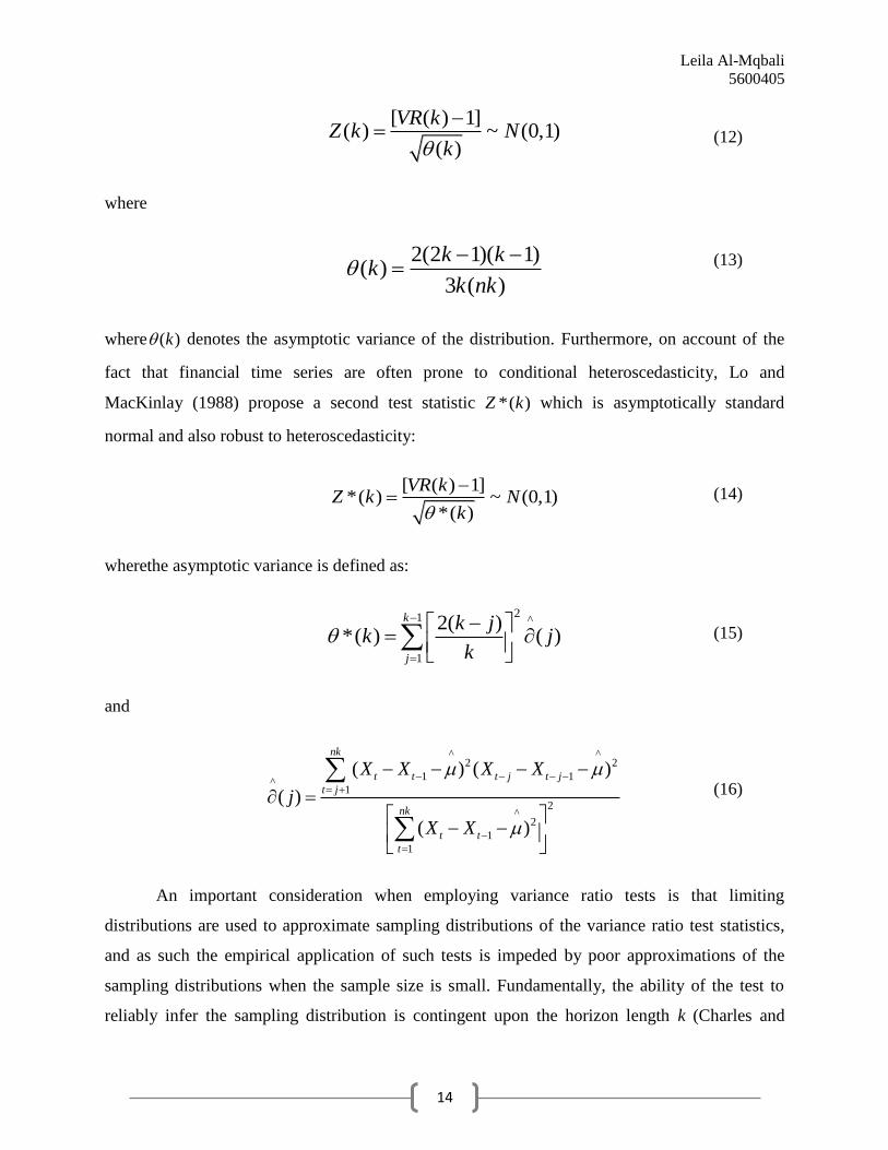
where ( )k denotes the asymptotic variance of the distribution. Furthermore, on account of the

fact that financial time series are often prone to conditional heteroscedasticity, Lo and

MacKinlay (1988) propose a second test statistic *( )Z k which is asymptotically standard

normal and also robust to heteroscedasticity:

[ ( ) 1]*( ) ~ (0,1)

*( )

VR kZ k N

k

wherethe asymptotic variance is defined as:

21 ^

1

2( )*( ) ( )

k

j

k jk j

k

and

^ ^2 2

1 1^

1

2^

2

1

1

( ) ( )

( )

( )

nk

t t t j t j

t j

nk

t t

t

X X X X

j

X X

An important consideration when employing variance ratio tests is that limiting

distributions are used to approximate sampling distributions of the variance ratio test statistics,

and as such the empirical application of such tests is impeded by poor approximations of the

sampling distributions when the sample size is small. Fundamentally, the ability of the test to

reliably infer the sampling distribution is contingent upon the horizon length k (Charles and

(12)

(13)

(14)

(15)

(16)

Leila Al-Mqbali

5600405

15

Darné, 2009, p.7). In particular, large k relative to the sample size has been shown to result in

biased and right skewed statistics (Lo and MacKinlay, 1989) which can weaken the power of the

test, and consequently Lo and MacKinlay recommend only employing the variance ratio test for

k ≤ 16. Noting that our primary analysis employs 1516 returns observations, we can therefore

deduce that any negative effects from this issue are minimal as 16/1516 yields a ratio of 0.0106.

Moreover, the Lo-MacKinlay variance ratio test investigates whether the variance ratio is

equal to unity for a particular horizon length, thereby rendering the method sequential in nature.

According to Chow and Denning (1993), assessing RWH for an individual value of kincreases

the probability of Type I error, since true randomness would require that the variance ratios

should equal one for all horizon lengths simultaneously. As a result, the Lo-MacKinlay variance

ratio test is often employed in conjunction with a multiple variance ratio test, in order to

ascertain the validity of RWH when various k are jointly subjected to the testing procedure.

Chow and Denning (1993) Multiple Variance Ratio Test

Extending the work on variance ratio tests favoured by Lo and MacKinlay, Chow and

Denning (1993) proposed a multiple variance ratio test which addressed the theoretical

challenges imposed by the sequential nature of the Lo-MacKinlay test. Following Hochberg’s

(1974) method for comparing a group of variance ratios for several distinct horizon lengths with

unity, Chow and Denning propose an empirical method for assessing RWH which controls for

the overall test size.

The null hypothesis under this test necessitates that each variance ratio in a set of m

estimates is jointly equal to one, and the null is rejected if any of the m estimated statistics is

statistically different from unity. More specifically, whereas the individual hypothesis test of Lo

and MacKinlay has null hypothesis ( ) ( ) 1 0rM k VR k , the joint hypothesis test of Chow and

Denning considers a set of m tests { ( ) | 1,2,..., }r iM k i m associated with a set of predetermined

lag lengths {ik | 1,2,...,i m },where the null and alternative hypotheses are as follows:

0 : ( ) 1i iH VR k for all 1,2,...,i m (17)

(18)

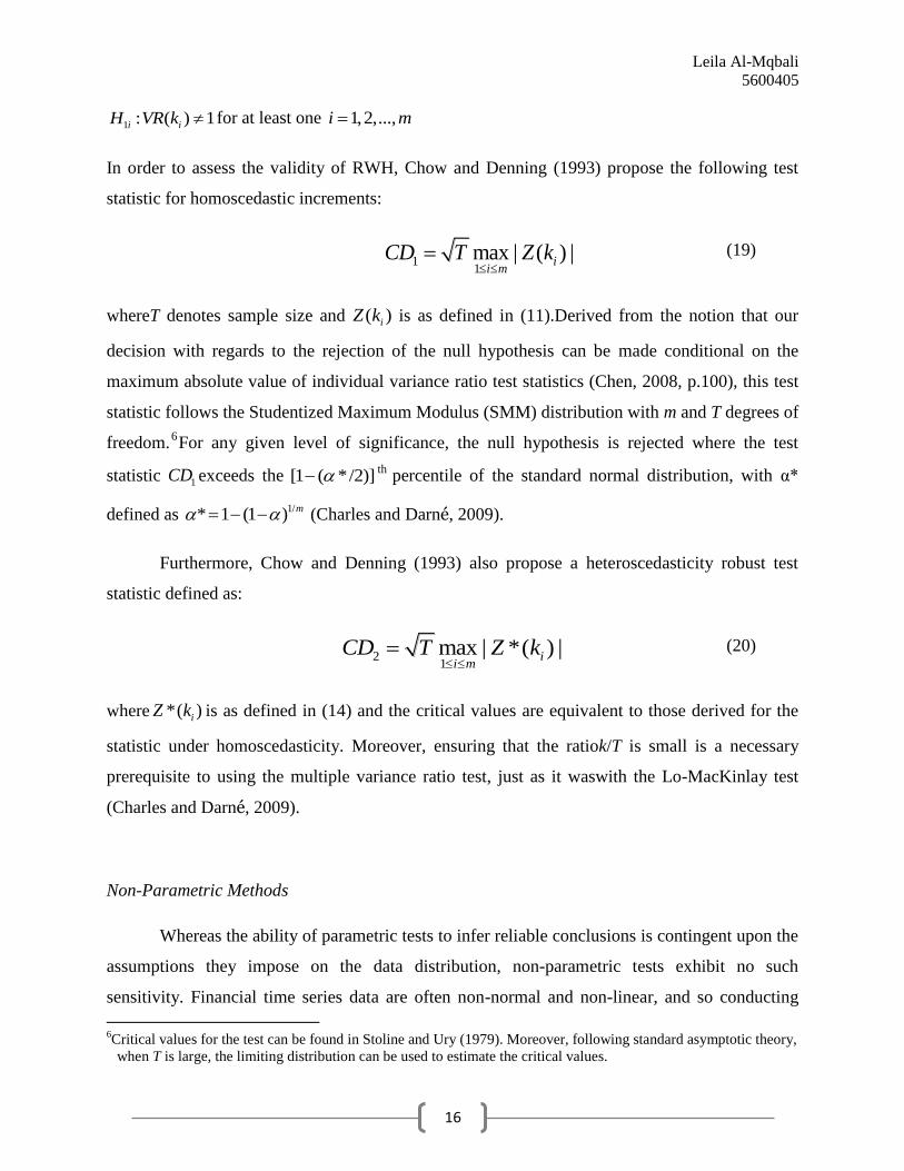
Leila Al-Mqbali

5600405

16

1 : ( ) 1i iH VR k for at least one 1,2,...,i m

In order to assess the validity of RWH, Chow and Denning (1993) propose the following test

statistic for homoscedastic increments:

11max | ( ) |i

i mCD T Z k

whereT denotes sample size and ( )iZ k is as defined in (11).Derived from the notion that our

decision with regards to the rejection of the null hypothesis can be made conditional on the

maximum absolute value of individual variance ratio test statistics (Chen, 2008, p.100), this test

statistic follows the Studentized Maximum Modulus (SMM) distribution with m and T degrees of

freedom.6For any given level of significance, the null hypothesis is rejected where the test

statistic 1CD exceeds the [1 ( */2)]th

percentile of the standard normal distribution, with α*

defined as 1/* 1 (1 ) m (Charles and Darné, 2009).

Furthermore, Chow and Denning (1993) also propose a heteroscedasticity robust test

statistic defined as:

21max | *( ) |i

i mCD T Z k

where *( )iZ k is as defined in (14) and the critical values are equivalent to those derived for the

statistic under homoscedasticity. Moreover, ensuring that the ratiok/T is small is a necessary

prerequisite to using the multiple variance ratio test, just as it waswith the Lo-MacKinlay test

(Charles and Darné, 2009).

Non-Parametric Methods

Whereas the ability of parametric tests to infer reliable conclusions is contingent upon the

assumptions they impose on the data distribution, non-parametric tests exhibit no such

sensitivity. Financial time series data are often non-normal and non-linear, and so conducting

6Critical values for the test can be found in Stoline and Ury (1979). Moreover, following standard asymptotic theory,

when T is large, the limiting distribution can be used to estimate the critical values.

(19)

(20)

Leila Al-Mqbali

5600405

17

empirical tests which do not impose restrictions on the returns distribution is warranted.

Furthermore, as discussed previously in SectionII, results from earlier studies have been shown

to be dependent upon the empirical methods employed by the researchers, and so conducting

parametric tests in conjunction with non-parametric tests increases the robustness of our results.

Runs Test

The runs test (Bradley, 1968) is one of the primary non-parametric methods used by

researchers to determine the validity of RWH. Siegel (1956) defines a run as “a succession of

identical symbols which are followed or preceded by different symbols or no symbol at all”

(p.52). In order to determine the validity of RWH, we can therefore characterize a run as the

succession of consecutive changes in the series of returns, and identify it as positive (negative)

wherever a sequence is positive (negative). Similarly, the run is zero if there are no changes in

the sequence (Hiremath, 2014, p. 27). The length of a run is delineated by the number of

consecutive positive, or negative, values.

In a truly random dataset, the probability of a run – that is, the likelihood that the (j +1)th

value will differ from the jth

value – follows a binomial distribution (NIST/SEMATECH, par.2).

Therefore, the total number of runs in the series serves as an indicator of the extent of

randomness, since an excessive tendency towards one particular type of run is itself indicative of

a trend (Muthotya, 2013, p. 50). If the number of runs is less than the expected number, this

reflects the overreaction of the market to new information (Poshokwale, 1996, p.89). Conversely,

a higher than expected number of runs suggests a delayed response to new information

(Muthotya, 2013, p.54). In order to test the null hypothesis that our data is generated by a

random process, we assess RWH by testing whether the total number of runs in our series is

statistically different from the number of runs expected in a random series containing the same

number of observations.

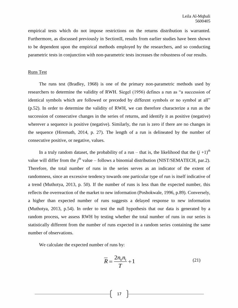
We calculate the expected number of runs by:

0 121

n nR

T

(21)

Leila Al-Mqbali

5600405

18

where 0n denotes the number of negative runs, 1n is the number of positive runs, and T is the total

number of observations. The Z-statistic is then computed by calculating:

R

R RZ

s

2 0 1 0 1 0 1

2

0 1 0 1

2 (2 )

( ) ( 1)R

n n n n n ns

n n n n

whereR is the number of actual runs and 2

RS is defined as the standard deviation of the returns

series. We then reject the null hypothesis of random returns if | |Z > 1 /2Z , where represents

the chosen level of significance. Small sample runs tests make use of critical values described in

Mendenall, Wackerly, and Scheaffer (2008). However, when the sample is large (i.e. when the

number of positive runs and negative runs each exceed ten) the test statistic can be approximated

as following a standard normal distribution.

The Brock, Dechert and Scheinkman (BDS) Test

Brock, Dechert, and Scheinkman (1987) developed a non-parametric method, commonly

known as the BDS test, to assess randomness in a dataset by detecting possible deviations from

independence. It is important to note that unlike the autocorrelation test which only has the

ability to detect linear dependence, the BDS test can detect various types of dependence,

including linear and non-linear dependence and chaos.7 Thus, failing to reject our null hypothesis

for the autocorrelation test does not necessarily mean that our data follows a random walk – only

that it does not exhibit linear dependence. In order to rule out other types of time-based

dependencies, the BDS test must also be conducted.

After anypossible linear structure has been removed from the time series by first

differencing or some other method of de-trending, the BDS test null hypothesis is that the

underlying data generating process is i.i.d. The alternative hypothesis allows for linear

dependence, non-linear dependence, and chaos. The theory behind the BDS test is rooted in the

7Characterized by intermittent periods of high volatility, chaotic processes are deterministic and non-linear processes

which can bear a similar resemblance to financial time series (Hsieh, 1991).

(22)

(23)

Leila Al-Mqbali

5600405

19

work on correlation integrals in time series pioneered by Grassberger and Procaccia (1983). The

discussion of the BDS test presented here closely follows Taylor (2005); the reader is

encouraged to consult this reference for further details and clarification.

For a sample of T observations {1,..., Tx x }, the correlation integral ( , )mC T must be

computed before the BDS test can be conducted on the returns observations. Denoting the

embedding dimension and the distance m and respectively, the equations are as follows:

1 if | |( , , )

0 otherwise

s t

s t

x xI x x

1

0

( , , ) ( , , )m

m s t s k t k

k

I x x I x x

1

1 1

2( , ) ( , , )

( )( 1)

T m T m

m m s t

s t s

C T I x xT m T m

where 1x ≤ sx ≤ Tx and 1x ≤ tx ≤ Tx . The function ( , , )s tI x x identifies whether the observations

at times s and t are close to each other at a given distance , and the product ( , , )m s tI x x is equal

to unity if and only if the two m-period histories 1 1( , ,..., )s s s mx x x and 1 1( , ,..., )t t t mx x x are

sufficiently close to each other such that each s kx is near t kx . Therefore, we can also define our

approximation of the correlation integral as the fraction of pairs of m-period histories that are

close to one another (Taylor, 2005, p.136).

As the sample size extends to infinity, observations from many processes define the limit

of correlation integrals as:

( ) lim ( , )m mT

C C T

If the data are indeed generated by an i.i.d. process, then the probability that a pair of

observations are near one another is the same for all possible combinations of data points, and

(24)

(25)

(26)

(27)

Leila Al-Mqbali

5600405

20

consequently the probability that there exists m consecutive near pairs is simply the product of

the equal probabilities:

1( ) ( )m

mC C

However, when the data generating process is chaotic, the conditional probability that s kx is

near to t kx , given that there has already been a near pair at some earlier time period j, is greater

than the unconditional probability and thus:

1( ) ( )m

mC C

Considering these properties of correlation integrals led Brock, Dechert, and Scheinkman

to study a random variable which, as the sample size increases, converges to a normal

distribution with mean zero and variance mV for i.i.d. processes. The BDS test statistic is

calculated as:

1( ) [ ( , ) ( , ) ]m

m m

m

TW C T C T

V

which has been demonstrated to be asymptotically standard normal (Brock, Hsieh, and Le Baron,

1991).^

mV represents a consistent estimator of the variance of the distribution and is given by:

1^2 2 2 2 2 2

1

4 ( 1) 2m

m m m m j jm

j

V K m C m KC K C

as discussed in Brock, Dechert, Scheinkman, and LeBaron (1996). Here, 1( , )C C T and K is

calculated as:

1 1

2 1 1

6( , , ) ( , , )

( 1)( )( 1)

T m s T m

m r s m s t

s r t s

K I x x I x xT m T m T m

,,,,

(28)

(29)

(30)

(31)

(32)

Leila Al-Mqbali

5600405

21

where ( , , )m s tI x x and ( , , )m r tI x x are as defined in (23) and (24). As demonstrated by Hsieh

(1991), with regards to detecting deviations from i.i.d. processes and alternative specifications,

the BDS test exhibits considerable power.Conventionally, the BDS test is conducted on the

sample of returns observations at several distinct m and ε, where ε assumes values between one

half and two times the standard deviation. Furthermore, it is generally accepted that a minimum

of 500 observations is required in order to infer reliable results from the BDS test (Abbas, 2014,

p.321) and that the accuracy of results diminishes for m≥5 (Brock et. al, 1991).

VI. Discussion of Empirical Results

Results from Autocorrelation Tests

Having previously confirmed the stationarity of the residual series, we plot the

autocorrelation functions using STATA computing software with a 5% significance level. As

shown in Figure 4, all lags except two (approximately lag 26 and lag 38)for the NASDAQ 100

are within the confidence bands, suggesting that the NASDAQ residual series do indeed follow a

white noise process. However, the ACF for the FTSE 100 has a number oflags significantly

outside the confidence bands, which could indicate that there is some degree of non-randomness

in the data.

In order to assess the overall randomness present in the time series, we apply the Ljung-

Box test. Previous studies investigating the RWH have found the significance of autocorrelations

to be dependent upon the chosen horizon length of the returns; conducting the Ljung-Box test

serves to investigate the joint null hypothesis that all autocorrelations are simultaneously equal to

zero.It is evident from the results in Table 5 that we cannot reject the null hypothesis for the

NASDAQ 100index at the five percent level of significance, as we obtain a p-value larger than

0.05. On the contrary, the null is rejected at the five percent level of significance (and indeed at

all conventional significance levels) for the FTSE 100, and thus we conclude from the Ljung-

Box test that all autocorrelations are not simultaneously equal to zero for the UK index. Put

differently, there appears to be some degree of serial correlation in the FTSE 100 residuals

Leila Al-Mqbali

5600405

22

series. Therefore, the results from the autocorrelations test appear to indicate that the RWH is

validated for the US index, but not the UK index.

Results from Lo-MacKinlay Variance Ratio Tests

The variance ratios VR(k) for both indices are computed by entering the raw data into

Microsoft Excel and inputting the necessary formulae. Recorded in the primary rows of Table 6,

the variance ratio for each index at each horizon level is approximately unity, although it is

readily apparent that the variance ratios for the NASDAQ 100 are marginally higher than those

reported for the FTSE 100 at each respective investment horizon. The horizon levels reported are

2, 4, 8, and 16, as is standard procedure when conducting Lo-MacKinlay tests.

Retrieved using R computing technology, the variance ratio homoscedastic test statistics

and heteroscedasticity robust test statistics for both indices are reported in the second and third

row parentheses of Table 6. The Lo-MacKinlay test dictates that the null hypothesis of random

fluctuations in returns should be rejected at the 5% level of significance wherever the absolute

value of the test statistic exceeds 1.96. Notably, we do not reject the null hypothesis for either

index at any of the standard investment horizons, supporting RWH in both the U.S. and U.K.

markets.

Results from Chow and Denning Multiple Variance Ratio Tests

In order to ensure the reliability of Lo-MacKinlay test results, the Chow and Denning

multiple variance ratio test is conducted. The objective of this exercise is to guarantee that the

null of RWH cannot be rejected even when we test the joint null hypothesis that the variance

ratios for all investment horizons simultaneously are not statistically different from unity. Recall

that the Chow and Denning multiple ratio test is only reliable when k/Tis small, where k denotes

the investment horizon and T represents sample size. Since the longest horizon length tested is 16

and the returns series contains 1540 observations, their ratio is approximately 0.01, and thus we

can proceed with the test.

Leila Al-Mqbali

5600405

23

Conducted once again using R computing software, the Chow and Denning

homoscedastic test statistics and heteroscedasticity robust test statistics are reported in Table 7.

Recall that the test statistics for the Chow and Denning test follow an SMM distribution. R

software generates these critical values electronically, and presents us with a critical value of

2.490915 at the 5% significance level. The test statistics for the FTSE 100 are markedly higher

than those reported for the NASDAQ 100 index; however, none of the statistics exceeds the

critical value of 2.490915, and so we cannot reject the null hypothesis for either index at the 5%

level of significance. Therefore, the results from the Chow and Denning multiple variance ratio

tests also support RWH in both markets.

Results from Runs Tests

In order to assess the robustness of the results to alternative empirical methods, we next

use STATA to perform the runs test; a non-parametric approach which tests whether the

residuals are mutually independent. Recall that if the data does indeed follow a random walk,

then the observations should be independent and identically distributed.

The results of the runs tests depicted in Table 8 reveal that the actual number of runs for

both indexes is very close to the number of runs that would be expected if the data were truly

generated by a random process. The negative Z-score for the FTSE 100 indicates that the

observed number of runs is less than the expected number, while the positive Z-score of the

NASDAQ 100 reflects that the observed number of runs is greater than the expected number.

However, since the Z-score for the UK index is greater than -1.96 and the Z-score for the US

index is less than 1.96, we cannot reject the null hypothesis that the residuals are independent at

the five percent level of significance for either index.

Results from BDS Tests

Finally, we conduct the BDS test for both indices in order to determine whether the

underlying data is generated by an i.i.d. process.In accordance with general procedure, we test

distances between one half and two times the standard deviation of the returnsseries, and we use

Leila Al-Mqbali

5600405

24

embedding dimensions between 2 and 5 (recall that conducting the test with dimensions greater

than five diminishes the reliability of the results).

Performed on the returns data series, R software reports the results for the NASDAQ 100

and the FTSE 100 BDS tests, which are summarized in Table 9 and Table 10 respectively. The

primary rows report the test statistics, while the values in parentheses denote the corresponding

p-values. The BDS test statistics are asymptotically standard normal, and once again we assess

the validity of the null hypothesis using a 5% significance level to maintain consistency with the

other empirical methods. From Table 9 and Table 10, each p-value is approximately zero and is

therefore less than the critical value of 0.05. Indeed, the BDS results are significant even at the

1% significance level for both indices. Consequently, the BDS test is the only test for which

RWH is strongly refuted for both the NASDAQ 100 and the FTSE 100.

VII. Summary and Discussion of the Empirical Results

The primary focus of this study was to investigate the validity of RWH for markets in two

countries with comparable economic development, market capitalization, and a similar number

of trading companies, in order to test how controlling for these factors impacted our results.

Analyzing weekly closing price data from October 1985 through April 2015 we find that

results broadly seem to support RWH in both markets. When subjected to the same three

parametric tests, we fail to reject the null hypothesis of randomness in all tests for the NASDAQ

100, and for two of the three tests for the FTSE 100. The only discrepancy in the results for the

parametric tests is that the FTSE 100 exhibits a statistically significant degree of correlation in

the returns series when subjected to the autocorrelation test.

With regards to non-parametric tests, we fail to reject the null hypothesis of random

returns for both indices when the Runs test is conducted. Conversely, when the BDS test is

performed, RWH is strongly refuted for both indices at all conventional levels of significance.

It is perhaps important to note that, typically, previous studies have strongly rejected RWH

when the data is subjected to the BDS test (Hsieh 1989, De Grauwe, Dewachter and Embrechts

Leila Al-Mqbali

5600405

25

1993, Steurer 1995, Brooks 1996). Some experts believe that this tendency may be due to the

fact that the BDS test is capable of detecting general dependence, whereas most statistical tests

are only capable of detecting linear dependence. Indeed, Lim, Azali, and Lee (2003)suggest that

it is the breakthroughs in non-linear dynamics and chaos theory which have prompted the

discovery of “dependencies in the underlying financial time series that often appear completely

random to standard linear statistical tests, such as serial correlation tests, non-parametric runs

tests, variance ratio tests and unit root tests” (p. 42).

Rejection of the null of an independent and identically distributed process implies that

there is some pattern in the behaviour of the stock prices that appears more frequently than one

would expect if the data were indeed truly generated by an i.i.d. process. However, at present,

existing empirical methods are not sophisticated enough to determine the exact cause of rejection

or indicate what pattern exists, if any. Further diagnostic tests, in particular non-parametric tests

which focus on non-linear dynamics, are warranted in order to infer more consistent and reliable

results.

Empirical analysis has shown that RWH is broadly supported for both the U.K. index and

the U.S. index, although improved testing procedures are needed to further investigate possible

nonlinear types of dependence. The following section will ascertain the robustness of our results

when various sub-periods of the sample data are used, and when alternative market indices are

employed in place of the FTSE 100 and the NASDAQ 100.

VIII. Robustness Analysis

In order to confirm that our results are consistent and reliable, we perform the parametric

and non-parametric tests once more with different stock market indices, using an alternative

observation horizon length, and using sub-samples of our original time series. If our results from

these further tests agree with our original findings in that they also broadly support RWH in both

markets, then we can conclude that our results appear robust to the choice of market indices,

horizon length,and the elected sample period.

Leila Al-Mqbali

5600405

26

Analyzing Alternative Indices

Data Selection and Stationarity

To ensure that the results from our empirical analysis are robust to the market indices, we

select another index from each market and repeat the testing procedures using weekly

observations across the same sample period. From the NASDAQ stock exchange market, we

select the NASDAQ Composite index. Also a capitalization weighted index, the NASDAQ

Composite contains data from several thousand companies and is weighted towards technology

companies. From the London Stock Exchange, we select the FTSE All-Share index, which is

again capitalization weighted and includes the majority of companies listed on the London Stock

Exchange.Summary statistics for the weekly closing prices of each alternative index are

illustrated in Table 11.

As expected, the raw price data from both indices exhibits a clear upwards trend, as is

evidenced from Figure 5.Performing the DF-GLS test confirms the non-stationarity of the U.S.

data, as we cannot reject the null hypothesis of a unit root at any conventional significance level

for any lag length of the NASDAQ Composite index. Furthermore, the results from the DF-GLS

tests also generally confirm the non-stationarity of the U.K. data, as we fail to reject the null

hypothesis for any lag length at the 1% and 5% levels of significance(although, at the 10% level

of significance we do reject the null at lags 2 and 23). The results are reportedin Table 12.

Having confirmed the non-stationarity of the price data, we once again compute the

returns and repeat the DF-GLS procedure. Summary statistics of the index weekly returns are

given in Table 13. From Figure 6 we can see that the returns data does appear to be stationary,

and in Table 14 the DF-GLS results confirm this, as we now reject the null hypothesis at all

significance levels and at all lag lengths for both indices.

Results from Parametric Tests

In order to determine whether the residual series of our alternative indices are correlated

over time, we once again perform the autocorrelations test. Figures 7 and 8 illustrate the residual

series and the autocorrelation functions of each index respectively. In contrast to our earlier

findings, it appears that there are more observations which lie outside the 95% confidence bands

Leila Al-Mqbali

5600405

27

for the NASDAQ Composite index than there were for the NASDAQ 100 index, and there are

also a significance number of data points outside the confidence bands for the FTSE All-Share

index. Performing the autocorrelation test yields p-values which are less than 0.05 for both

indices, indicating thatRWH is rejected at the 5% significance level. Conveyed in Table 15, there

appears to be some degree of serial correlation in the residual series for both of our alternative

indices, and therefore the autocorrelations testsdo not support RWH in either market.

Conducting the Lo-MacKinlay variance ratio test once morepresents us with results

similar to those obtained when the NASDAQ 100 and FTSE 100 indices were tested. Table 16

reports the variance ratios for the NASDAQ Composite and the FTSE All-Share in the primary

rows, while the values in the second and third row parentheses denote the homoscedastic test

statistic and the heteroscedasticity robust test statistic respectively. With regards to the FTSE

All-Share, we cannot reject the null of random returns at the 5% significance level for any

investment horizon as we obtain test statistics whose absolute value is less than 1.96.

Furthermore, the only statistic to be rejected for the NASDAQ Composite index is the statistic

for homoscedastic increments at a horizon length of 8, and consequently the results obtained

from the Lo-MacKinlay tests on alternative indices closely resemble the results acquired from

our original tests.

We next perform the Chow andDenning multiple variance ratio test in order to assess the

joint null hypothesis that all variance ratios simultaneously are not statistically different from

unity. Once again, our critical value is 2.490915 at the 5% level of significance as our test

statistic follows a SMM distribution.Table 17 presents the results from the Chow and Denning

multiple variance ratio test, and it is clear that we cannot reject the null hypothesis for either

index since the test statistics for homoscedastic increments and the heteroscedasticity robust test

statistics all have an absolute value less than the critical value. Consequently, the results from the

Chow and Denning test also support RWH for both of our alternative indices.

Results from Non-Parametric Tests

Proceeding now to non-parametric methods, Table 18 reports the results from the runs

tests. For both the NASDAQ Composite and the FTSE All-Share, it appears that the observed

number of runs is less than the expected number if the data were truly random, as is evidenced

Leila Al-Mqbali

5600405

28

by the negative Z-scores of each index. However, we cannot reject the null hypothesis of random

returns at the 5% significance level since both Z-scores obtained are less than 1.96 in terms of

absolute value. Therefore, the results from the runs tests also defend the validity of RWH in both

financial markets.

We perform the BDS test once more for our alternative indices using the same range of

values for the distance and embedding dimensions as previously employed in this paper. The

results are documented in Tables 19 and 20. The primary rows report the test statistics whilst the

values in parentheses denote the corresponding p-values. Yet again, the p-values are

approximately zero for both of our alternative indices and therefore the BDS results reject the

null of randomness at all conventional significance levels in both the UK and US markets.

Conclusions from Alternative Indices

Clearly, with the exception of the results from the autocorrelations tests, the results from

testing alternative indices broadly agree with the results from analyzing our initial data. With our

original indices we find that results from autocorrelations tests support RWH in the NASDAQ

but not in the FTSE; however when we subject our alternative indices to the autocorrelations

tests we find that there is no support for RWH in either market.

Interestingly, the NASDAQ 100 does not include financial securities such as those from

investment companies in its calculations, whilst the NASDAQ Composite index does not

discriminate against such securities. Therefore, one possible reason for the discrepancy in the

results from the autocorrelations tests is that the presence of large financial and investment

companies in the NASDAQ Composite index are driving the behaviour of the index, thereby

causing the autocorrelations to be more pronounced over time. Furthermore, the NASDAQ

Composite index has a strong focus on technology firms, and it is possible that the stock prices

of these large technology companies may be more likely to exhibit common patterns that can

cause the index to become more autocorrelated during some of the phases of the business cycle.

The results from the rest of the parametric tests and from the non-parametric tests on our

alternative indices all closely follow the results obtained from our original indices. RWH is once

again supported by the Lo-MacKinlay test, the Chow and Denning test, and the runs test, while

Leila Al-Mqbali

5600405

29

strongly rejected by the BDS test. As discussed earlier, it is possible that this rejection may be

due to some underlying non-linear deterministic behaviourwarranting further investigation.

Overall, it appears that our results seem to be largely unaffected by the choice of index, and that

RWH is generally valid for our chosen markets with similar economic development and market

capitalization.

Adjusting the Horizon Length of Observations

Data and Stationarity

As a second robustness check, we adjust the horizon length of the returns data for our

original indices. Our tests thus far have employed a sample of weekly observations for each

index. Data are also available for monthly and daily time intervals. Since using monthly data

would significantly reduce the number of observations in our sample, we collect daily data which

will serve to increase our sample size dramatically. However, as discussed previously, we must

consider that potential biases may become statistically significant with the use of daily

observation intervals.

Conveyed in Table 21 are summary statistics for the daily price data for the NASDAQ

100 and FTSE 100indices. Despite the fact that our horizon length is now much shorter than

before, the mean and standard deviations of the raw price data are close to those retrieved from

our original weekly observations. The DF-GLS test results are given in Table 22, and once again

we cannot reject the null hypothesis of a unit root for either index at any significance level.

Computing daily returns in an attempt to retrieve a time series that is stationary yields summary

statistics presented in Table 23, and after performing the DF-GLS test once more for both indices

we can now reject the null at all conventional levels of significance. These results are illustrated

in Table 24.

Results from Parametric Tests

Now that our data is confirmed to be stationary we can conduct the autocorrelation tests

on the return residuals for both indices. Displayed in Table 25, the analysis generates p-values

Leila Al-Mqbali

5600405

30

that are once again less than 0.05 for each index, and so we reject the RWH for both indices at

the 5% level of significance using daily horizon returns. Indeed, the results are significant even

at the1% significance level.

Results from the Lo-MacKinlay tests for each index are depicted in Table 26. The null of

random returns cannot be rejected at the 5% significance level for the FTSE 100 index at any

investment horizon, which agrees with our results using weekly observation intervals. However,

for the NASDAQ 100 index we now reject the null hypothesis at the 5% significance level at

horizons 4 and 8 (for both the statistic for homoscedastic increments and the heteroscedasticity

robust statistic) and also at horizon16 (for the homoscedastic statistic). This is in contrast to our

earlier results using weekly data where we could not reject the null hypothesis at the 5% level for

any investment horizon. Therefore, the analysis from the Lo-MacKinlay tests yield mixed results

regarding the validity of RWH: random returns seem to be supported in the UK market while

broadly refuted in the US market for all investment horizons greater than 2.

Performing the Chow and Denning tests we find further evidence of mixed empirical

results. Presented in Table 27, we find that we cannot reject the null hypothesis at the 5% level

for the FTSE 100 index, which again agrees with our results from weekly observation intervals.

Conversely, the null for the homoscedastic NASDAQ 100 test statistic is rejected at the 5% level

of significance, whereas when weekly observations were employed earlier in the paper we could

not reject the null at the 5% level.

Results from Nonparametric Tests

The runs test results and BDS test results for daily observation intervals do not support

the RWH for either index. Conducting the runs tests reveals that the number of runs for each

index was less than the expected number, as is evidenced by the negative Z-scores in Table 28.

Moreover, the Z-scores for both indices were significantly greater than 1.96 in terms of absolute

value and thus we strongly reject the null hypothesis of random returns at the 5% significance

level. In addition, the results from the BDS tests given in Table 29 and Table 30 reveal that – as

with weekly observations and the use of alternative indices – we strongly reject the null

hypothesis of random returns at all conventional significance levels for both indices.

Leila Al-Mqbali

5600405

31

Conclusions from Daily Observation Intervals

After close analysis of the data using daily observation intervals, we observe that our

results do not appear robust to the modified horizon length. Although conclusions from the

autocorrelations tests, Chow and Denning tests, and BDS tests agree with our previous analysis,

results from the Lo-MacKinlay and runs tests diverge from those derived from our original

investigation.Using daily horizon intervals the runs test now refutes RWH in both markets,

whereas when weekly observation intervals were employed, the results supported random returns

for each index. With regards to the Lo-MacKinlay tests, whereas our original analysis found

support for RWH in both markets, employing daily observation intervals provides mixed results.

Specifically, the results from the Lo-MacKinlay test on the FTSE 100 index is unaffected by the

modified horizon length, however we now reject the null for the NASDAQ 100 at all investment

horizons larger than 2.

Therefore, employing daily observations as opposed to weekly observations reveals

ambiguous results with regards to the validity of random walk in the stock market. Conclusions

drawn from the autocorrelation tests, runs tests, and BDS tests refute random walk for both

markets, results from the Chow and Denning tests support random walk for both markets, and

results from the Lo-MacKinlay tests are mixed. However, itis quite possible that this ambiguity

is due to latent biases becoming statistically significant with the shorter observation interval, as

discussed previously.

In particular, consider that the shortest investment horizon for the Lo-MacKinlay test

with weekly observation intervals was 14 days, while the longest horizon was 112 days. In

contrast, using daily observations implies that our longest horizon is just 16 days –

approximately the same length as the shortest horizon employed in our primary analysis.

Therefore, all empirical tests which involve the use of investment horizons cover a significantly

different length of time relative to the baseline scenario. It follows that a difference in results is

not entirely unexpected.

Leila Al-Mqbali

5600405

32

Sub-sampling Original Data

Lastly, we draw subsamples of our original datasets for the NASDAQ 100 and the FTSE

100 in order to assess whether our findings are dependent on the choice of sample period. We do

this by eliminating all observations from the original datasets which are related to periods of

economic crises, and create subsamples setting the break to be the beginning of a recessionary

period.

Justification

Constructing such modified samples where we remove all observations related to

recessionary periods is justified for several reasons. Periods of crises are associated with greater

insecurity in a number of markets, and this increased market instability is generally reflected by

an increase in the volatility of stock market indices. The intuition behind this is simple: once an

economy enters recession, firms either profit less from their investments or suffer losses,

resulting in lower dividends paid to investors. This decrease in dividend payments consequently

renders stocks less attractive assets.

It is possible that the behaviour of stock prices during recessionary periods is responding

to increased uncertainty in the financial and economic markets, and therefore stock returns

cannot possibly be fluctuating completely at random. For this reason, we eliminate all

observations pertaining to major economic crises and instead evaluate whether, under general

economic conditions, RWH is valid for the U.S. and U.K. markets.

Identification of Financial Crises

During the course of the original sample period (October 1st

1985-April 13th

2015) there

were three major recessionary periods in the United States: the early 1990s recession, the early

2000s recession, and the Great Recession of 2007-2008. The United Kingdom also experienced

recessions in the early 1990s and in 2007-2008; however the UK managed to avoid the recession

in the early 2000s. As we noted earlier in section IV, from Figure 3 there appears to be a large

disturbance around the year 2000 in the NASDAQ 100 residuals that is not readily apparent in

Leila Al-Mqbali

5600405

33

the residuals for the FTSE 100.8 It is likely that this inconsistency in residual pattern is, at least in

part, due to the fact that the recession of 2000-2001 was not felt in the United Kingdom. In

addition, it is worth noting that the fact that two of these three major economic events were

common to both countries serves to underscore the mounting significance of globalization and

also highlights the increasing importance of financial markets.

Lasting from July 1990 through March 1991 in the United States (Walsh, C.E., 1993) and

from July 1990 through September 1991 in the United Kingdom (Chamberlin, G., 2010), the

early 1990s recession was largely due to decreased consumer confidence resulting from rising oil

prices following Iraq’s invasion of Kuwait, the savings and loans crisis, and the stock market

crash of 1987. Following this economic downturn, the U.S. economy then experienced further

crisis from March 2001 – November 2001 (NBER, 2003), largely due to the dot-com crash and

the 9/11 attacks. Finally, due to the subprime mortgage crisis and subsequent global financial

meltdown, the U.S. encountered recession from December 2007 – June 2009 (NBER, 2010) and

the U.K. was in recession from June 2008 – September 2009 (Chamberlin, G., 2010).

Data and Stationarity

Removing these dates from our original sample periods, we then create subsamples of

weekly observations for the US and UK markets. After eliminating all data points related to the

recessionary periods delineated above, we set the break between subsamples to be the start of a

recession. Specifically, we obtain 4 subsamples for the NASDAQ 100, and 3subsamples for the

FTSE 100 index. Summary statistics detailing these sub-periods of raw price data are presented

in Table 31. The DF-GLS test results for the price data of subsamples of each index are

portrayed in Tables 33 and 35. Once again, the null of a unit root in the price data cannot be

rejected at any conventional significance level for the NASDAQ 100 index. For the FTSE 100,

we cannot reject the null in two of the three subsamples, the exception being the third sub-period

where the results are significant at least at the 10% level for all lag lengths. It may be that the

small sample size of 289 observations is responsible for this unexpected result.

8We also noted earlier that there is a significant outlier in the NASDAQ 100 series around the year 1994; however, this does not appear to coincide with any period of major financial crisis.

Leila Al-Mqbali

5600405

34

In order to conduct our empirical analysis, the data must be stationary and so we compute

the returns for each index subsample, and report the summary statistics in Table 32. Performing

the DF-GLS test once more, as is evidenced from Tables 34 and Table 36, we can now reject the

null of a unit root at the 1% level for most lags of each subsample of the NASDAQ 100 and

FTSE 100 indices. The only exceptions are the 3rd

subsample of the NASDAQ 100 index (where

we can only reject at the 1% significance level for lags 1,2, and 4) and the 4th

subsample of the

NASDAQ 100 index(where we can only reject at the 1% significance level for lags 1 and

2).Therefore, we can conclude thatour data generally appears to be stationary, and we can

proceed with our empirical tests.

Results from Parametric Tests

Table 37 presents the results from conducting the autocorrelations test on the residuals of

each index subsample.For the NASDAQ 100 index, the only statistically significant result at the

5% level is the third sub-period containing 308 observations. The p-values for all other

subsamples are much larger than 0.05, indicating that for these sub-periods there does not appear

to be a high degree of serial correlation in the residuals over time. Noting the small sample size

of the third sub-period and that the results for all other subsamples are not significant, we

conclude that our results from the autocorrelations tests on the NASDAQ 100 generally appear to

support RWH in contrast to our earlier findings.

For subsamples of the FTSE 100 index, we find ambiguous results. The first subsample,

consisting of 248 observations, is significant at the 5% level which indicates a high degree of

correlation in the residuals. Conversely, the second and third sub-periods, containing 868 and

289 observations respectively, are not significant at the 5% level.It is possible that these

conflicting results are due to the relatively small sample size of some of the sub-periods, or else

due to some underlying effect caused by the removal of observations relating to periods of

financial crises. Furthermore, it is important to note that the number of observations employed in

the tests will actually be smaller than the number of data points in our original subsample. This

is due to the fact that several of the tests involve using lags of the variable, thereby reducing the

number of observations.

Leila Al-Mqbali

5600405

35

The Lo-MacKinlay test results for subsamples seem to broadly agree with our original

findings for both indices, as is evidenced from Table 38. Generally, the null hypothesis cannot be

rejected at the 5% level: the only exceptions are the third sub-period for the NASDAQ 100

where we reject the null of randomness at investment horizons 8 and 16, the first sub-period for

the FTSE 100 where we reject the null at investment horizon 4, and the third sub-period for the

FTSE 100 where we reject the null at horizons 8 and 16. Otherwise, our analysis closely

resembles the results retrieved using the original samples for each index.

Employing the Chow and Denning multiple variance ratio tests also yields results similar

to our original findings, as is evidenced in Table 39. The null hypothesis of random returns

cannot be rejected for any subsample of the NASDAQ 100 index, and is rejected only for the

first subsample of the FTSE 100 index. Again, it is likely that this rejection is due to the small

sample size.

Results from Non-Parametric Tests

Table 40 reports the results from the runs tests performed on each subsample of index

returns. For both indices, we find that we cannot reject the null of randomness at the 5% level for

any subsample, as the absolute value of the Z-scores is less than 1.96 for each period.

Results from the BDS tests for subsamples of the NASDAQ 100 and FTSE 100 are

conveyed in Table 41 and Table 42, respectively. Once more, the BDS test proves robust to

alternative specifications of the data, and again refutes RWH for both markets. The only cases

for which randomness cannot be rejected are presented in red, and pertain to the sub-periods

containing the smallest number of observations.

Conclusions from Sub-sampling Original Data

Evidently, our original analysis appears to be generally robust to the choice of sample

period, as testing sub-periods of our original data yields similar conclusions. Results from the

Lo-MacKinlay tests, Chow and Denning tests, and runs tests on subsamples broadly agree with

the conclusions from testing the entire sample period, in that RWH is supported for both

Leila Al-Mqbali

5600405

36

markets. Furthermore, the BDS test once again refutes random walk for both indices, and the

autocorrelations tests offers mixed conclusions, as was the case in our original investigation.

IX. Conclusions and Recommendations for Future Research

The purpose of this paper was to assess whether stock prices in two well developed

markets with high market capitalization follow a random walk, in order to determine whether

controlling for these dynamics produces consistent results with regards to the validity of RWH.

Using a consistent number of observations across the same sample period, we subjected the

NASDAQ 100 and FTSE 100 indices to a variety of empirical tests in an attempt to assess the

validity of RWH in each market. Both parametric and non-parametric techniques were employed

in order to gauge the robustness of the results to empirical methods, particularly since previous

literature has found results to be dependent upon the empirical approach.

Our primary results from testing weekly observations from each index suggested that

randomness was broadly supported for both markets. However, the autocorrelation test results

were mixed, as RWH was supported for the NASDAQ 100 while refuted for the FTSE. Notably,

the BDS test was the only method to strongly reject RWH for both indices.

Indeed, when subjecting our analysis to a number of robustness checks, the BDS test

continued to strongly reject random returns for all alternative data specifications. The robustness

checks included using different stock market indices for each market, using daily returns as

opposed to weekly returns, and using subsamples of our original dataset.

Employing alternative market indices and sub-sampling our original sample period

generated results which closely resembled our original findings; however, the autocorrelations

tests for the alternative indices rejected random walk in both marketsas opposed to providing

mixed evidence. Conversely, our original findings were not robust to the use of daily observation

intervals. Using daily horizons, results from the Lo-MacKinlay tests became mixed, and the runs

tests refuted RWH for both markets.

Leila Al-Mqbali

5600405

37

Thus, when our original dataset is modified to assess the robustness of our empirical

results,the only tests to offer consistent and reliable conclusions are the BDS and Chow and

Denning tests. However, since the results from these tests directly oppose each other, this fact

provides little insight. Since the use of alternative indices and subsamples leaves our original

findings largely unchanged, it is possible that the discrepancies in results when assessing daily

horizon returns are due to underlying biases becoming statistically significant with shorter

observation intervals. Advanced research and statistical methods are needed to further investigate

these inconsistencies. In particular, additional means of testing for non-linear dependence in time

series are warranted. Future research must work to develop new means of testing for randomness

in datasets, as at present, empirical investigations of random walk are not robust to the

techniques employed.

Furthermore, the fact that our results for each index are not robust to the horizon interval

suggests that the diversity in professional opinion regarding the validity of RWH cannot be

wholly attributed to differences in market capital and economic development. Further research

should attempt to control for other factors when testing the legitimacy of RWH in stock prices,

such as trading frequency and volume, with the aim of identifying key economic dynamics

which influence the results.

Leila Al-Mqbali

5600405

38

References

Abbas, Ghada. (2014). Testing Random Walk Behaviour in the Damascus Securities Exchange.

International Journal of Academic Research in Accounting, Finance and Management

Sciences.4(4):317-325. DOI:10.6007/IJARAFMS/v4-i4/1368

Bachelier, Louis (2006). Theory of Speculation: Origins of Modern Finance. (M. Davis and A.

Etheridge, Trans.).Princeton, NJ: Princeton University Press. (original work published in 1900).

Bradley, James V. (1968). Distribution-Free Statistical Tests. Englewood Cliffs, NJ: Prentice-

Hall Inc.

Brock, W. A., W. D. Dechert, and J. A. Scheinkman (1987). A Test for Independence Based On

the Correlation Dimension.Department of Economics, University of Wisconsin at Madison,

University of Houston, and University of Chicago.

Brock, W., Hsieh, D., and Le Baron, B. (1991).Nonlinear Dynamics, Chaos, and Instability:

Statistical Theory and Economic Evidence.MIT Press.

Brock, W. A., Dechert, W. D., Scheinkman, J. A. and LeBaron, B. (1996). A Test for

Independence Based on the Correlation Dimension. Econometric Reviews.15(3).

Brooks, C. (1996). Testing for Non-linearity in Daily Sterling Exchange Rates.Applied Financial

Economics. 6:307-317

Butler,Kirt C., and Malaikah, S.J. (1992). Efficiency and Inefficiency in Thinly Traded Stock

Markets: Kuwait and Saudi Arabia. Journal of Banking Finance. 16(1):197–210.

Campbell, J.Y., Lo, A.W., and MacKinlay, A.C. (1997).The Econometrics of Financial Markets.

Princeton, NJ: Princeton University Press.

Chamberlin, Graeme. (2010). Output and Expenditure in the Last Three UK

Recessions.Economic and Labour Market Review. 4(8): 51-64

Charles, Amélie, and Darné, Olivier. (2009). Variance Ratio Tests of Random Walk: An

Overview. Journal of Economic Surveys. 23(3): 503–527.

Leila Al-Mqbali

5600405

39

Chen, Jeng-Hong. (2008). Variance Ratio Tests of Random Walk Hypothesis of the Euro

Exchange Rate. International Business and Economics Research Journal. 7(12): 97-105.

Chow, K.V. and Denning, K.C. (1993). A Simple Multiple Variance Ratio Test. Journal of

Econometrics. 58: 385–401.

Cooper, J.C.B. (1982). World Stock Markets: Some Random Walk Tests. Applied

Economics.14(5): 515–531.

Cootner, Paul H. (1962).Stock Prices: Random vs. Systematic Changes.Industrial Management

Review.3(2): 24–45.Chow K.V., and Denning K.C. (1993.) A Simple Multiple Variance Ratio

Test. Journal of Econometrics. 58(3):385–401.

De Grauwe, P., Dewachter H., and Embrechts, M. (1993).Exchange Rate Theory: Chaotic

Models of Foreign Exchange Markets. Oxford: Blackwell.

Dickinson, J.P. and Muragu, K. (1994). Market Efficiency in Developing Countries: A Case

Study of the Nairobi Stock Exchange. Journal of Business Finance and Accounting 21(1): 133-

150.

Elliott, Graham., Rothenberg, Thomas R., and Stock, James. (1996). Efficient Tests for an

Autoregressive Unit Root. Econometrica. 64(4): 813-836.

Fama, Eugene F. (1965). The Behavior of Stock Market Prices.Journal of Business. 38(1):34–

106.

Fama, Eugene F., and French, Kenneth R. (1988).Permanent and Temporary Components of

Stock Prices.Journal of Political Economics. 96(2): 246-273.

Grassberger, Peter, and Procaccia, Itamar.(1983). Characterization of Strange Attractors.Physical

Review Letters. 50(5):340-346.

Hiremath, Gourishankar S. (2014). Indian Stock Market.Springer India. DOI: 10.1007/978-81-

322-1590-5_2.

Hochberg, Y. (1974). Some Conservative Generalizations of the T-method in Simultaneous

Inference.Journal of Multivariate Analysis. 4: 224-234.

Leila Al-Mqbali

5600405

40

Hsieh, David A. (1989). Testing for Non-Linearity in Dinly Foreign Exchange Rate

Changes.Journal of Business. 62: 339-368.

Hsieh, David A. (1991). Chaos and Nonlinear Dynamics: Application to Financial Markets. The

Journal of Finance.46(5):1839-1877.

Lim, K.P., Azali, M., and Lee, H.A. (2003). Is MYR/USD a Random Walk? New Evidence from

the BDS Test. Pertanika Journal of Social Science and Humanities. 11(1): 41-49

Ljung, Greta M., and Box, George E.P. (1978).On A Measure of Lack of Fit in Time Series

Models.Biometrika. 65: 297-303.

Lo, Andrew W., and MacKinlay, Craig A. (1988). Stock Markets do not Follow Random Walks:

Evidence from a Simple Specification Test. The Review of Financial Studies.1(1):41-66.

Lo, Andrew W., and MacKinlay, Craig A. (1989). The Size and Power of the Variance Ratio

Test in Finite Samples: A Monte Carlo Investigation. Journal of Econometrics. 40: 203-238.

Lo, Andrew W., andMacKinlay, Craig A. (2002). ANon-Random Walk Down Wall

Street.Princeton, NJ: Princeton University Press.

Malkiel, Burton G. (2003).The Efficient Market Hypothesis and Its Critics.Journal of Economic

Perspectives.17(1):59-82.

Malkiel, Burton G. (2007).A Random Walk Down Wall Street. New York, NY: W. W. Norton

Company, Inc.

Mbululu, D., Auret, C.J., and Chiliba, L. (2014). Do Exchange Rates Follow Random Walks? A

Variance Ratio Test of the Zambian Foreign Exchange Market.Southern African Business

Review. 17(2):45-66.

Mendenall, W., Wackerly, D., and Scheaffer,R.L. (2007). Mathematical Statistics with

Applications (7th

ed.).Cengage Learning.

Mustafa,Khalid, and Nishat, Mohammed. (2007). Testing for Market Efficiency in Emerging

Markets: a Case Study of Karachi Stock Market. Lahore Journal of Economics. 12(1):119–140.

Leila Al-Mqbali

5600405

41

Mutothya, Nicholas. (2013). An Empirical Investigation of the Random Walk Hypothesis of

Stock Prices on the Nairobi Stock Exchange. European Journal of Accounting Audtiting and

Finance Research. 1(4): 33-59.

National Bureau of Economic Research.(2003). Business Cycle Dating Committee. Retrieved

July 10th

2015 from: http://www.nber.org/cycles/july2003.html

National Bureau of Economic Research.(2010). Business Cycle Dating Committee. Retrieved

July 10th

2015 from: http://www.nber.org/cycles/sept2010.html

NIST/SEMATECH e-Handbook of Statistical Methods.Retrieved June 29th

2015 from

http://www.itl.nist.gov/div898/handbook/eda/section3/eda35d.htm

Osborne M.F.M. (1959). Brownian Motion in the Stock Market. Operations Research.7(2):145-

173.

Poshakwale, S. (1996).Evidence on the Weak-form Efficiency and the Day of the Week Effect in

the Indian Stock Market. Finance India. 10(3): 605-616.

Praetz, P. D. (1969). Australian Share Prices and the Random Walk Hypothesis.Australian

Journal of Statistics.11(3): 123-139. doi:10.1111/j.1467-842X.1969.tb00100.x

Samuels, J. M. (1981). Inefficient Capital Markets and their Implications.in F.G.J. Derkinders

and R.L. Crum(eds.), Risk Capital Costs and Project Financing Decisions(pp.129-148).Martinus

Nijhof: Boston/TheHauge/London.

Samuelson, Paul A.(1965). Proof that Properly Anticipated Prices Fluctuate Randomly.

Industrial Management Review. 6(2): 41–49.

Schwert, G.W. (1989). Tests for Unit Roots: A Monte Carlo Investigation. Journal of Business

and Economics Statistics. 7: 147-159.

Siegel, Sidney, (1956). Non-parametric Statistics for Behavioral Sciences. New York: McGraw-

Hill Company.

Solnik, Bruno H. (1973). Note on the Validity of the Random Walk for European Stock Prices.

Journal of Finance. 28(5):1151–1159.

Leila Al-Mqbali

5600405

42

Statistica. (2015). http://www.statistica.com/statistics/270127/largest-stock-exchanges-

worldwide-by-trading-volume

Steurer, E. (1995). Nonlinear Modeling of the DEM/USD Exchange Rate. In Neural Networks in

the Capital Markets, ed. A.P. Refenes. pp. 199-211. New York: John Wiley and Sons.

Stoline, M.R., and Ury, H. K. (1979).Tables of the Studentized Maximum Modulus Distribution

and an Application to Multiple Comparisons among Means. Technometrics. 21: 87–93.

Taylor, Stephen, J. (1986). Modelling Financial Time Series.New York: John Wiley.

Taylor, Stephen, J. (2005). Asset Price Dynamics, Volatility, and Prediction. New

Jersey:Princeton University Press.

Walsh, C.E. (1993). What Caused the 1990-1991 Recession? Economic Review of the Federal

Reserve Bank of San Francisco.2: 34–48.

World Federation of Exchanges. (2015). http://www.world-exchanges.org/statistics

Leila Al-Mqbali

5600405

43

Appendix A: Data Sources

Data Source

Weekly Closing Price Data

for the NASDAQ 100

NASDAQ 100 Historical Prices. Obtained from the NASDAQ via:

https://www.google.ca/finance/historical?q=INDEXNASDAQ%3ANDXandei=Dp6

BVfmiEYGH2Aa_4YKoDw

Weekly Closing Price Data

for the FTSE 100

FTSE 100 Historical Prices. Obtained from the LSE via:

https://www.google.ca/finance/historical?q=INDEXFTSE%3AUKXandei=rp6BVZi

YH8O72Aa7h4DwBw

Weekly Closing Price Data

for the NASDAQ

Composite

NASDAQ Composite Historical Prices. Obtained from the NASDAQ via:

https://www.google.ca/finance/historical?q=INDEXNASDAQ%3A.IXICandhl=enan

dei=YX69VfnpI5TwjAHxxqf4Dg

Weekly Closing Price Data

for the FTSE All-Share

FTSE All-ShareHistorical Prices. Obtained from the LSE via:

https://www.google.ca/finance/historical?q=INDEXFTSE%3AASXandhl=enandei=t

H69VejLE5bLjAHQ7IbAAw

Daily Closing Price Data for

the NASDAQ 100

NASDAQ 100 Historical Prices. Obtained from the NASDAQ via:

https://www.google.ca/finance/historical?q=INDEXNASDAQ%3ANDXandei=vH2

9VaHUGMStjAHclbnoDg

Daily Closing Price Data for

the FTSE 100

FTSE 100 Historical Prices. Obtained from the LSE via:

https://www.google.ca/finance/historical?q=INDEXFTSE%3AUKXandhl=enandei=

IX69VdmUNYjHjAGpkoeADw

Leila Al-Mqbali

5600405

44

0

200

04

00

06

00

08

00

0

FT

SE

10

0 C

losin

g P

rices

1985w1 1990w1 1995w1 2000w1 2005w1 2010w1 2015w1

Date

FTSE 100 Weekly Closing Prices

0

200

04

00

06

00

08

00

0

NA

SD

AQ

100

Clo

sin

g P

rice

s

1985w1 1990w1 1995w1 2000w1 2005w1 2010w1 2015w1Date

NASDAQ 100 Weekly Closing Prices

Appendix B: Plots and Figures

Figure 1: Index Closing Prices

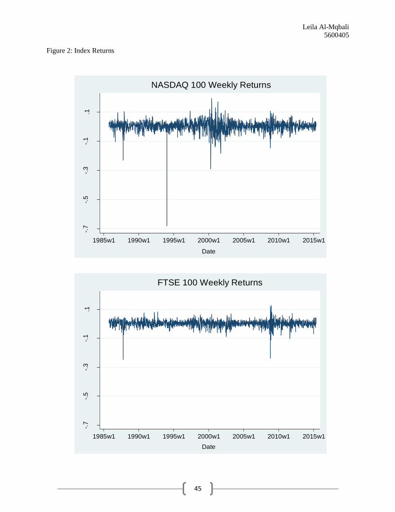
Leila Al-Mqbali

5600405

45

-.7

-.5

-.3

-.1

.1

FT

SE

10

0 R

etu

rns

1985w1 1990w1 1995w1 2000w1 2005w1 2010w1 2015w1

Date

FTSE 100 Weekly Returns

-.7

-.5

-.3

-.1

.1

NA

SD

AQ

100

Retu

rns

1985w1 1990w1 1995w1 2000w1 2005w1 2010w1 2015w1

Date

NASDAQ 100 Weekly Returns

Figure 2: Index Returns

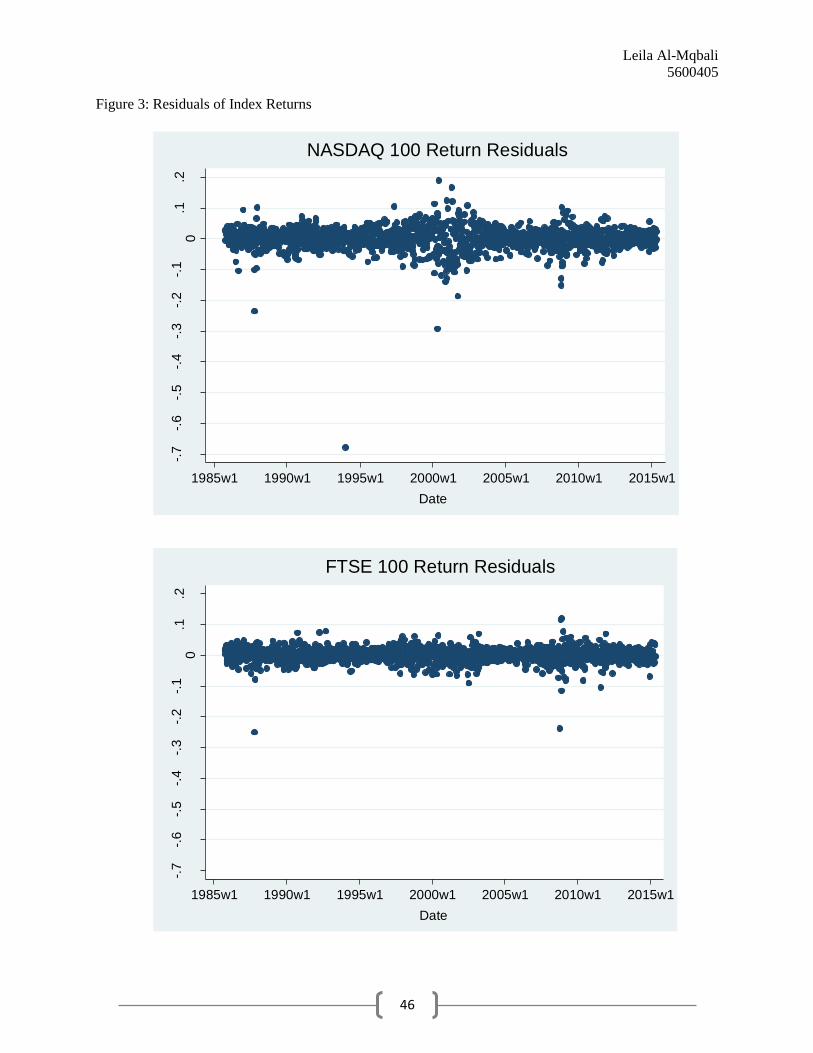
Leila Al-Mqbali

5600405

46

-.7

-.6

-.5

-.4

-.3

-.2

-.1

0.1

.2

FT

SE

10

0 R

esid

ua

ls

1985w1 1990w1 1995w1 2000w1 2005w1 2010w1 2015w1

Date

FTSE 100 Return Residuals

-.7

-.6

-.5

-.4

-.3

-.2

-.1

0.1

.2

NA

SD

AQ

100

Resid

uals

1985w1 1990w1 1995w1 2000w1 2005w1 2010w1 2015w1

Date

NASDAQ 100 Return Residuals

Figure 3: Residuals of Index Returns

Leila Al-Mqbali

5600405

47

-0.1

0-0

.05

0.0

00

.05

0.1

0

Resid

ual A

uto

corr

ela

tion

s

0 10 20 30 40

Lags

Bartlett's formula for MA(q) 95% confidence bands

FTSE 100 Autocorrelation Function

-0.0

50

.00

0.0

5-0

.10

0.1

0

Resid

ual A

uto

corr

ela

tion

s

0 10 20 30 40

Lags

Bartlett's formula for MA(q) 95% confidence bands

NASDAQ 100 Autocorrelation Function

Figure 4: Index Autocorrelation Functions

Leila Al-Mqbali

5600405

48

0

100

02

00

03

00

04

00

05

00

0

FT

SE

All-

Sha

re C

losin

g P

rices

1985w1 1990w1 1995w1 2000w1 2005w1 2010w1 2015w1

Date

FTSE All-Share Weekly Closing Prices

0

100

02

00

03

00

04

00

05

00

0

NA

SD

AQ

Com

posite

Clo

sin

g P

rices

1985w1 1990w1 1995w1 2000w1 2005w1 2010w1 2015w1

Date

NASDAQ Composite Weekly Closing Prices

Figure 5: Alternative Index Closing Prices

Leila Al-Mqbali

5600405

49

-.3

-.2

-.1

0.1

.2

FT

SE

All-

Sha

re R

etu

rns

1985w1 1990w1 1995w1 2000w1 2005w1 2010w1 2015w1

Date

FTSE All-Share Weekly Returns

-.3

-.2

-.1

0.1

.2

NA

SD

AQ

Com

posite

Retu

rns

1985w1 1990w1 1995w1 2000w1 2005w1 2010w1 2015w1

Date

NASDAQ Composite Weekly Returns

Figure 6: Alternative Index Returns

Leila Al-Mqbali

5600405

50

-.3

-.2

-.1

0.1

.2

NA

SD

AQ

Com

posite

Retu

rns

1985w1 1990w1 1995w1 2000w1 2005w1 2010w1 2015w1

Date

NASDAQ Composite Return Residuals-.

3-.

2-.

10

.1.2

FT

SE

All-

Sha

re R

etu

rns

1985w1 1990w1 1995w1 2000w1 2005w1 2010w1 2015w1

Date

FTSE All-Share Returns

Figure 7: Residuals of Alternative Index Returns

Leila Al-Mqbali

5600405

51

-0.1

0-0

.05

0.0

00

.05

0.1

0

Resid

ual A

uto

corr

ela

tion

s

0 10 20 30 40

Lags

Bartlett's formula for MA(q) 95% confidence bands

NASDAQ Composite Autocorrelation Function

-0.1

0-0

.05

0.0

00

.05

0.1

0

Resid

ual A

uto

corr

ela

tion

s

0 10 20 30 40

LagsBartlett's formula for MA(q) 95% confidence bands

FTSE All-Share Autocorrelation Function

Figure 8: Alternative Index Autocorrelation Functions

Leila Al-Mqbali

5600405

52

Appendix C: Tables

Table 1: Summary Statistics for Index Weekly Closing Prices

Index Observations Mean Standard

Deviation

Min Max

NASDAQ 100 1541 1444.5530 1031.1950 220.1500 4691.6100

FTSE 100 1541 4390.6910 1656.8070 1313.0000 7089.8000

Table 2: DF-GLS Tests for Index Weekly Closing Prices

Index Number of

Lags

DF-GLS Test

Statistic for Index

Weekly Prices

1%

Critical

Value

5%

Critical

Value

10%

Critical

Value

NASDAQ

100

23 –1.939 –3.480 –2.830 –2.544

20 –1.813 –3.480 –2.833 –2.546

16 –1.972 –3.480 –2.837 –2.550

15 –2.018 –3.480 –2.838 –2.551

8 –1.480 –3.480 –2.844 –2.557

4 –1.413 –3.480 –2.848 –2.560

2 –1.431 –3.480 –2.850 –2.562

1 –1.413 –3.480 –2.851 –2.562

FTSE 100

23 –2.196 –3.480 –2.830 –2.544

22 –2.018 –3.480 –2.831 –2.545

16 –2.018 –3.480 –2.837 –2.550

13 –1.904 –3.480 –2.840 –2.553

8 –1.975 –3.480 –2.844 –2.557

4 –2.033 –3.480 –2.848 –2.560

2 –2.266 –3.480 –2.850 –2.562

1 –2.153 –3.480 –2.851 –2.562 NASDAQ 100: Maximum lag for the index is 23, selected by the Schwert Criterion. The Ng-Perron criterion selects 20 as the optimal lag, while

the SC criterion and MAIC criterion choose 1 and 15 respectively. FTSE 100: Maximum lag for the index is 23, selected by the Schwert Criterion. The Ng-Perron criterion selects 22 as the optimal lag, while the

SC criterion and MAIC criterion choose 1 and 13 respectively.

Note: The null hypothesis is rejected at the α% level of significance wherever the DF-GLS test statistic ≤ α% critical value. Values marked with *, **, and *** denote significance at the 10%, 5%, and 1% levels respectively.

Table 3: Summary Statistics for Index Weekly Returns

Index Observations Mean Standard

Deviation

Min Max

NASDAQ 100 1540 0.0019 0.0387 – 0.6770 0.1914

FTSE 100 1540 0.0011 0.0239 – 0.2486 0.1258

Leila Al-Mqbali

5600405

53

Table 4: DF-GLS Tests for Index Weekly Returns

Index Number of

Lags

DF-GLS Test

Statistic for Index

Weekly Prices

1%

Critical

Value

5%

Critical

Value

10%

Critical

Value

NASDAQ

100

23 –7.070 *** –3.480 –2.830 –2.544

16 –8.510 *** –3.480 –2.837 –2.550

10 –10.531 *** –3.480 –2.843 –2.555

8 –12.469 *** –3.480 –2.844 –2.557

4 –16.104 *** –3.480 –2.848 –2.560

2 –21.883 *** –3.480 –2.850 –2.562

1 –26.890 *** –3.480 –2.851 –2.562

FTSE 100

23 –6.751 *** –3.480 –2.830 –2.544

22 –6.630 *** –3.480 –2.831 –2.545

21 –6.832 *** –3.480 –2.832 –2.546

16 –8.567 *** –3.480 –2.837 –2.550

8 –13.377 *** –3.480 –2.844 –2.557

4 –7.229 *** –3.480 –2.848 –2.560

2 –22.682 *** –3.480 –2.850 –2.562

1 –25.418 *** –3.480 –2.851 –2.562 NASDAQ 100: Maximum lag for the index is 23, selected by the Schwert Criterion. The Ng-Perron criterion selects 10 as the optimal lag, while the SC criterion and MAIC criterion choose 1 and 23 respectively.

FTSE 100: Maximum lag for the index is 23, selected by the Schwert Criterion. The Ng-Perron criterion selects 21 as the optimal lag, while the

SC criterion and MAIC criterion choose 1 and 22 respectively. Note: The null hypothesis is rejected at the α% level of significance wherever the DF-GLS test statistic ≤ α% critical value. Values marked with

*, **, and *** denote significance at the 10%, 5%, and 1% levels respectively.

Table 5: Autocorrelation Test Results for Index Weekly Returns

Index Returns Number of Lags Ljung Box Q-Statistic P-Value

NASDAQ 100 40 34.8051 0.7028

FTSE 100 40 89.6936 0.0000

The number of lags is chosen conventionally as k=min(T/2 – 2, 40) where T denotes the number of observations. The null hypothesis is

rejected at the 5% level of significance wherever the p-value ≤ 0.05.

Table 6: Lo and MacKinlay Variance Ratio Test Statistics for Index Weekly Returns

Index Returns

2 4 8 16

0.9856 1.0016 1.0610 1.1275

NASDAQ 100 (–0.5894) (–0.0098) (0.7446) (1.0387)

(–0.4461) (–0.0077) (0.5979) (0.8394)

0.9545 0.9848 0.9406 0.8399

FTSE 100 (–1.7402) (–0.3216) (–0.8218) (–1.4863)

(–1.2868) (–0.2215) (–0.5472) (–0.9867) The variance ratios VR(k) are reported in the primary rows, while the test statistic for homoscedastic increments Z(k) and the heteroscedasticity

robust test statistic Z*(k) are given in the second and third row parentheses respectively. Asterisked values indicate rejection of the random

walk hypothesis at the 5% level of significance, i.e. wherever the |Z-statistic| ≥ 1.96.

Lo and MacKinlay Variance Ratios for Various Investment Horizons

Leila Al-Mqbali

5600405

54

Table 7: Chow and Denning Multiple Variance Ratio Test Statistics for Index Returns

Index Returns Homoscedastic Statistic Heteroscedastic Statistic

NASDAQ 100 1.038719 0.839373

FTSE 100 1.740174 1.286797 The 5% critical value is 2.490915, and so we reject the null hypothesis if |Z-statistic| ≥ 2.490915. Asterisked values indicate rejection of random

walk hypothesis at the 5% level of significance.

Table 8: Runs Test Statistics for Index Returns

Index Returns Residuals ≤ 0 Residuals > 0 Expected

Runs

Actual

Runs

Z-Score Prob>|z|

NASDAQ 100 713 826 766 788 1.11 0.27

FTSE 100 721 818 767 752 –0.79 0.43 The null hypothesis rejected at the 5% level of significance if | Z-score | ≥ 1.96.

Table 9: BDS Test Statistics for NASDAQ 100 Index Weekly Returns

Distance (𝛆)

2 3 4 5

0.5S 10.4805 (0.0000) 12.6378 (0.0000) 15.3339 (0.0000) 18.1596 (0.0000)

1.0S 11.7339 (0.0000) 14.3461 (0.0000) 16.4868 (0.0000) 18.3048 (0.0000)

1.5S 12.2136 (0.0000) 14.9902 (0.0000) 16.8608 (0.0000) 18.0126 (0.0000)

2.0S 12.1134 (0.0000) 14.3052 (0.0000) 15.9673 (0.0000) 16.8336 (0.0000)

𝛆,m, and S denote the distance, dimension, and standard deviation respectively. 𝛆 is calculated as various multiples (0.5, 1, 1.5, and 2) of the standard deviation of the data. The primary rows report the BDS test statistics for the NASDAQ index, while the values in parentheses yield the corresponding p-values. The test statistic is asymptotically standard normal, and so the null hypothesis is rejected at the 5% level of

significance where the p-value ≤ 0.05.

Table 10: BDS Test Statistics for FTSE 100 Index Weekly Returns

Distance (𝛆)

2 3 4 5

0.5S 6.1624 (0.0000) 9.2907 (0.0000) 11.1658 (0.0000) 13.1169 (0.0000)

1.0S 6.4578 (0.0000) 9.4122 (0.0000) 10.7497 (0.0000) 12.2003 (0.0000)

1.5S 6.1119 (0.0000) 8.9963 (0.0000) 9.9877 (0.0000) 10.9656 (0.0000)

2.0S 5.4647 (0.0000) 8.2492 (0.0000) 9.0695 (0.0000) 9.7359 (0.0000)

𝛆,m, and S denote the distance, dimension, and standard deviation respectively. 𝛆 is calculated as various multiples (0.5, 1, 1.5, and 2) of the standard deviation of the data. The primary rows report the BDS test statistics for the London Stock Exchange index, while the values in

parentheses yield the corresponding p-values. The test statistic is asymptotically standard normal, and so the null hypothesis is rejected at the

5% level of significance where the p-value ≤ 0.05.

Dimension (m)

Dimension (m)

Leila Al-Mqbali

5600405

55

Table 11: Summary Statistics for Alternative Index Weekly Closing Prices

Index Observations Mean Standard

Deviation

Min Max

NASDAQ

Composite

1541 1760.7790 1153.2670 280.5000 5048.6200

FTSE

All-Share

1541 2196.5700 854.9778 625.7500 3830.8700

Table 12: DF-GLS Tests for Alternative Index Weekly Closing Prices

Index Number of

Lags

DF-GLS Test

Statistic for Index

Weekly Prices

1%

Critical

Value

5%

Critical

Value

10%

Critical

Value

NASDAQ

Comp.

23 –1.832 –3.480 –2.830 –2.544

16 –1.960 –3.480 –2.837 –2.550

15 –1.986 –3.480 –2.838 –2.551

8 –1.692 –3.480 –2.844 –2.557

4 –1.741 –3.480 –2.848 –2.560

2 –1.748 –3.480 –2.850 –2.562

1 –1.641 –3.480 –2.851 –2.562

FTSE

All-Share

23 –2.575 * –3.480 –2.830 –2.544

22 –2.541 –3.480 –2.831 –2.545

16 –2.409 –3.480 –2.837 –2.550

13 –2.233 –3.480 –2.840 –2.553

8 –2.294 –3.480 –2.844 –2.557

4 –2.319 –3.480 –2.848 –2.560

2 –2.583 * –3.480 –2.850 –2.562

1 –2.421 –3.480 –2.851 –2.562 NASDAQ Comp.: Maximum lag for the index is 23, selected by the Schwert Criterion. The Ng-Perron criterion selects 15 as the optimal lag, while the SC criterion and MAIC criterion choose 1 and 15 respectively.

FTSE All-Share: Maximum lag for the index is 23, selected by the Schwert Criterion. The Ng-Perron criterion selects 22 as the optimal lag,

while the SC criterion and MAIC criterion choose 1 and 13 respectively. Note: The null hypothesis is rejected at the α% level of significance wherever the DF-GLS test statistic ≤ α% critical value. Values marked with

*, **, and *** denote significance at the 10%, 5%, and 1% levels respectively.

Table 13: Summary Statistics for Alternative Index Weekly Returns

Index Observations Mean Standard

Deviation

Min Max

NASDAQ

Composite

1540 0.0019 0.0304 – 0.2918 0.1738

FTSE

All-Share

1540 0.0012 0.0232 – 0.2536 0.1211

Leila Al-Mqbali

5600405

56

Table 14: DF-GLS Tests for Alternative Index Weekly Returns

Index Number of

Lags

DF-GLS Test

Statistic for Index

Weekly Returns

1%

Critical

Value

5%

Critical

Value

10%

Critical

Value

NASDAQ

Comp.

23 –7.973 *** –3.480 –2.830 –2.544

16 –9.211 *** –3.480 –2.837 –2.550

8 –12.911 *** –3.480 –2.844 –2.557

6 –14.149 *** –3.480 –2.846 –2.559

5 –13.957 *** –3.480 –2.847 –2.559

4 –16.054 *** –3.480 –2.848 –2.560

2 –21.617 *** –3.480 –2.850 –2.562

1 –25.930 *** –3.480 –2.851 –2.562

FTSE

All-Share

23 – 6.726 *** –3.480 –2.830 –2.544

22 –6.583 *** –3.480 –2.831 –2.545

21 –6.811 *** –3.480 –2.832 –2.546

16 –8.435 *** –3.480 –2.837 –2.550

8 –13.014 *** –3.480 –2.844 –2.557

4 –16.829 *** –3.480 –2.848 –2.560

2 –22.083 *** –3.480 –2.850 –2.562

1 –24.385 *** –3.480 –2.851 –2.562 NASDAQ Comp.: Maximum lag for the index is 23, selected by the Schwert Criterion. The Ng-Perron criterion selects 6 as the optimal lag, while the SC criterion and MAIC criterion choose 1 and 5 respectively.

FTSE All-Share: Maximum lag for the index is 23, selected by the Schwert Criterion. The Ng-Perron criterion selects 21 as the optimal lag,

while the SC criterion and MAIC criterion choose 1 and 22 respectively. Note: The null hypothesis is rejected at the α% level of significance wherever the DF-GLS test statistic ≤ α% critical value. Values marked with

*, **, and *** denote significance at the 10%, 5%, and 1% levels respectively.

Table 15: Autocorrelation Test Results for Alternative Index Returns

Index Returns Number of Lags Ljung Box Q-Statistic P-Value

NASDAQ Composite 40 61.9059 0.0147

FTSE All-Share 40 94.5642 0.0000

The number of lags is chosen conventionally as k=min(T/2 – 2, 40) where T denotes the number of observations. The null hypothesis is

rejected at the 5% level of significance wherever the p-value ≤ 0.05.

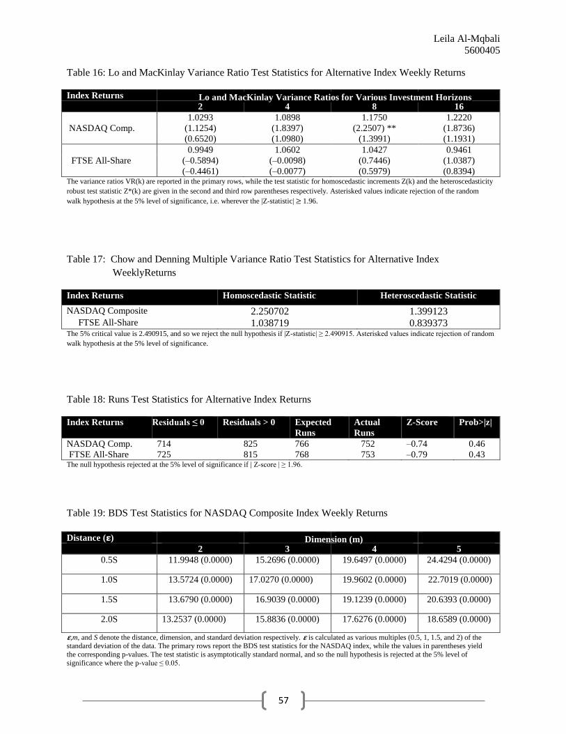
Leila Al-Mqbali

5600405

57

Table 16: Lo and MacKinlay Variance Ratio Test Statistics for Alternative Index Weekly Returns

Index Returns

2 4 8 16

1.0293 1.0898 1.1750 1.2220

NASDAQ Comp. (1.1254) (1.8397) (2.2507) ** (1.8736)

(0.6520) (1.0980) (1.3991) (1.1931)

0.9949 1.0602 1.0427 0.9461

FTSE All-Share (–0.5894) (–0.0098) (0.7446) (1.0387)

(–0.4461) (–0.0077) (0.5979) (0.8394) The variance ratios VR(k) are reported in the primary rows, while the test statistic for homoscedastic increments Z(k) and the heteroscedasticity

robust test statistic Z*(k) are given in the second and third row parentheses respectively. Asterisked values indicate rejection of the random

walk hypothesis at the 5% level of significance, i.e. wherever the |Z-statistic| ≥ 1.96.

Table 17: Chow and Denning Multiple Variance Ratio Test Statistics for Alternative Index

WeeklyReturns

Index Returns Homoscedastic Statistic Heteroscedastic Statistic

NASDAQ Composite 2.250702 1.399123 FTSE All-Share 1.038719 0.839373 The 5% critical value is 2.490915, and so we reject the null hypothesis if |Z-statistic| ≥ 2.490915. Asterisked values indicate rejection of random

walk hypothesis at the 5% level of significance.

Table 18: Runs Test Statistics for Alternative Index Returns

Index Returns Residuals ≤ 0 Residuals > 0 Expected

Runs

Actual

Runs

Z-Score Prob>|z|

NASDAQ Comp. 714 825 766 752 –0.74 0.46

FTSE All-Share 725 815 768 753 –0.79 0.43 The null hypothesis rejected at the 5% level of significance if | Z-score | ≥ 1.96.

Table 19: BDS Test Statistics for NASDAQ Composite Index Weekly Returns

Distance (𝛆)

2 3 4 5

0.5S 11.9948 (0.0000) 15.2696 (0.0000) 19.6497 (0.0000) 24.4294 (0.0000)

1.0S 13.5724 (0.0000) 17.0270 (0.0000) 19.9602 (0.0000) 22.7019 (0.0000)

1.5S 13.6790 (0.0000) 16.9039 (0.0000) 19.1239 (0.0000) 20.6393 (0.0000)

2.0S 13.2537 (0.0000) 15.8836 (0.0000) 17.6276 (0.0000) 18.6589 (0.0000)

𝛆,m, and S denote the distance, dimension, and standard deviation respectively. 𝛆 is calculated as various multiples (0.5, 1, 1.5, and 2) of the standard deviation of the data. The primary rows report the BDS test statistics for the NASDAQ index, while the values in parentheses yield

the corresponding p-values. The test statistic is asymptotically standard normal, and so the null hypothesis is rejected at the 5% level of

significance where the p-value ≤ 0.05.

Lo and MacKinlay Variance Ratios for Various Investment Horizons

Dimension (m)

Leila Al-Mqbali

5600405

58

Table 20: BDS Test Statistics for FTSE All-Share Index Weekly Returns

Distance (𝛆)

2 3 4 5

0.5S 10.4805 (0.0000) 12.6378 (0.0000) 15.3339 (0.0000) 18.1596 (0.0000)

1.0S 11.7339 (0.0000) 14.3461 (0.0000) 16.4868 (0.0000) 18.3048 (0.0000)

1.5S 12.2136 (0.0000) 14.9902 (0.0000) 16.8608 (0.0000) 18.0126 (0.0000)

2.0S 12.1134 (0.0000) 14.3052 (0.0000) 15.9673 (0.0000) 16.8336 (0.0000)

𝛆,m, and S denote the distance, dimension, and standard deviation respectively. 𝛆 is calculated as various multiples (0.5, 1, 1.5, and 2) of the standard deviation of the data. The primary rows report the BDS test statistics for the NASDAQ index, while the values in parentheses yield

the corresponding p-values. The test statistic is asymptotically standard normal, and so the null hypothesis is rejected at the 5% level of significance where the p-value ≤ 0.05.

Table 21: Summary Statistics for Index Daily Closing Prices

Index Observations Mean Standard

Deviation

Min Max

NASDAQ 100 10787 1441.7400 1026.6390 214.3200 4704.7300

FTSE 100 10787 4384.4450 1654.0890 1296.0000 7089.8000

Table 22: DF-GLS Tests for Index Daily Closing Prices

Index Number of

Lags

DF-GLS Test

Statistic for Index

Daily Prices

1%

Critical

Value

5%

Critical

Value

10%

Critical

Value

NASDAQ

100

38 –1.642 –3.480 –2.835 –2.548

8 –1.266 –3.480 –2.839 –2.551

4 –1.419 –3.480 –2.839 –2.551

2 –1.575 –3.480 –2.840 –2.552

1 –1.584 –3.480 –2.840 –2.552

FTSE 100

38 –2.041 –3.480 –2.835 –2.548

35 –2.044 –3.480 –2.836 –2.548

8 –2.137 –3.480 –2.844 –2.557

4 –2.250 –3.480 –2.848 –2.560

2 –2.425 –3.480 –2.850 –2.562

1 –2.403 –3.480 –2.851 –2.562 NASDAQ 100: Maximum lag for the index is 38, selected by the Schwert Criterion. The Ng-Perron criterion, the SC criterion, and the MAIC

criterion also select 38 as the optimal lag, while the SC criterion chooses 1 lag as optimal. FTSE 100: Maximum lag for the index is 38, selected by the Schwert Criterion. The Ng-Perron criterion selects 35 as the optimal lag, while the

SC criterion and MAIC criterion choose 4 and 35 respectively.

Note: The null hypothesis is rejected at the α% level of significance wherever the DF-GLS test statistic ≤ α% critical value. Values marked with *, **, and *** denote significance at the 10%, 5%, and 1% levels respectively.

Dimension (m)

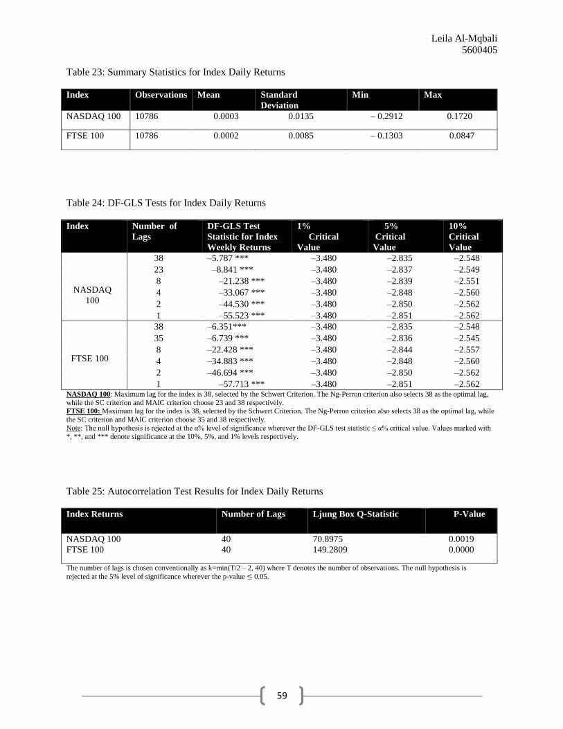
Leila Al-Mqbali

5600405

59

Table 23: Summary Statistics for Index Daily Returns

Index Observations Mean Standard

Deviation

Min Max

NASDAQ 100 10786 0.0003 0.0135 – 0.2912 0.1720

FTSE 100 10786 0.0002 0.0085 – 0.1303 0.0847

Table 24: DF-GLS Tests for Index Daily Returns

Index Number of

Lags

DF-GLS Test

Statistic for Index

Weekly Returns

1%

Critical

Value

5%

Critical

Value

10%

Critical

Value

NASDAQ

100

38 –5.787 *** –3.480 –2.835 –2.548

23 –8.841 *** –3.480 –2.837 –2.549

8 –21.238 *** –3.480 –2.839 –2.551

4 –33.067 *** –3.480 –2.848 –2.560

2 –44.530 *** –3.480 –2.850 –2.562

1 –55.523 *** –3.480 –2.851 –2.562

FTSE 100

38 –6.351*** –3.480 –2.835 –2.548

35 –6.739 *** –3.480 –2.836 –2.545

8 –22.428 *** –3.480 –2.844 –2.557

4 –34.883 *** –3.480 –2.848 –2.560

2 –46.694 *** –3.480 –2.850 –2.562

1 –57.713 *** –3.480 –2.851 –2.562 NASDAQ 100: Maximum lag for the index is 38, selected by the Schwert Criterion. The Ng-Perron criterion also selects 38 as the optimal lag,

while the SC criterion and MAIC criterion choose 23 and 38 respectively. FTSE 100: Maximum lag for the index is 38, selected by the Schwert Criterion. The Ng-Perron criterion also selects 38 as the optimal lag, while

the SC criterion and MAIC criterion choose 35 and 38 respectively.

Note: The null hypothesis is rejected at the α% level of significance wherever the DF-GLS test statistic ≤ α% critical value. Values marked with *, **, and *** denote significance at the 10%, 5%, and 1% levels respectively.

Table 25: Autocorrelation Test Results for Index Daily Returns

Index Returns Number of Lags Ljung Box Q-Statistic P-Value

NASDAQ 100 40 70.8975 0.0019

FTSE 100 40 149.2809 0.0000

The number of lags is chosen conventionally as k=min(T/2 – 2, 40) where T denotes the number of observations. The null hypothesis is

rejected at the 5% level of significance wherever the p-value ≤ 0.05.

Leila Al-Mqbali

5600405

60

Table 26: Lo and MacKinlay Variance Ratio Test Statistics for Index Daily Returns

Index Returns

2 4 8 16

0.9846 0.9249 0.8857 0.8630

NASDAQ 100 (–1.3386) (–3.4812) ** (–3.3572) ** (–2.7191) **

(–0.8844) (–2.2780) ** (–2.2262) ** (–1.8454)

1.000164 0.9396 0.9051 0.9170

FTSE 100 (–0.5894) (–0.0100) (–0.7446) (–1.0387)

(–0.4461) (–0.0077) (–0.5979) (–0.8394) The variance ratios VR(k) are reported in the primary rows, while the test statistic for homoscedastic increments Z(k) and the heteroscedasticity

robust test statistic Z*(k) are given in the second and third row parentheses respectively. Asterisked values indicate rejection of the random

walk hypothesis at the 5% level of significance, i.e. wherever the |Z-statistic| ≥ 1.96.

Table 27: Chow and Denning Multiple Variance Ratio Test Statistics for Index Daily Returns

Index Returns Homoscedastic Statistic Heteroscedastic Statistic

NASDAQ 100 3.481191 ** 2.278031

FTSE 100 1.038719 0.8393733 The 5% critical value is 2.490915, and so we reject the null hypothesis if |Z-statistic| ≥ 2.490915. Asterisked values indicate rejection of random

walk hypothesis at the 5% level of significance.

Table 28: Runs Test Statistics for Index Daily Returns

Index Returns Residuals ≤ 0 Residuals > 0 Expected

Runs

Actual

Runs

Z-Score Prob>|z|

NASDAQ 100 5224 5561 5388 4024 –26.3 0.00

FTSE 100 5554 5231 5389 4185 –23.2 0.00 The null hypothesis rejected at the 5% level of significance if | Z-score | ≥ 1.96.

Table 29: BDS Test Statistics for NASDAQ 100 Index Daily Returns

Distance (𝛆)

2 3 4 5

0.5S 18.3725 (0.0000) 26.7738 (0.0000) 33.6127 (0.0000) 42.3939 (0.0000)

1.0S 21.9768 (0.0000) 30.7533 (0.0000) 36.1855 (0.0000) 41.9352 (0.0000)

1.5S 24.2540 (0.0000) 32.8442 (0.0000) 37.3409 (0.0000) 41.3468 (0.0000)

2.0S 24.4371 (0.0000) 32.5397 (0.0000) 36.4054 (0.0000) 39.4711 (0.0000)

𝛆,m, and S denote the distance, dimension, and standard deviation respectively. 𝛆 is calculated as various multiples (0.5, 1, 1.5, and 2) of the standard deviation of the data. The primary rows report the BDS test statistics for the NASDAQ index, while the values in parentheses yield

the corresponding p-values. The test statistic is asymptotically standard normal, and so the null hypothesis is rejected at the 5% level of

significance where the p-value ≤ 0.05.

Lo and MacKinlay Variance Ratios for Various Investment Horizons

Dimension (m)

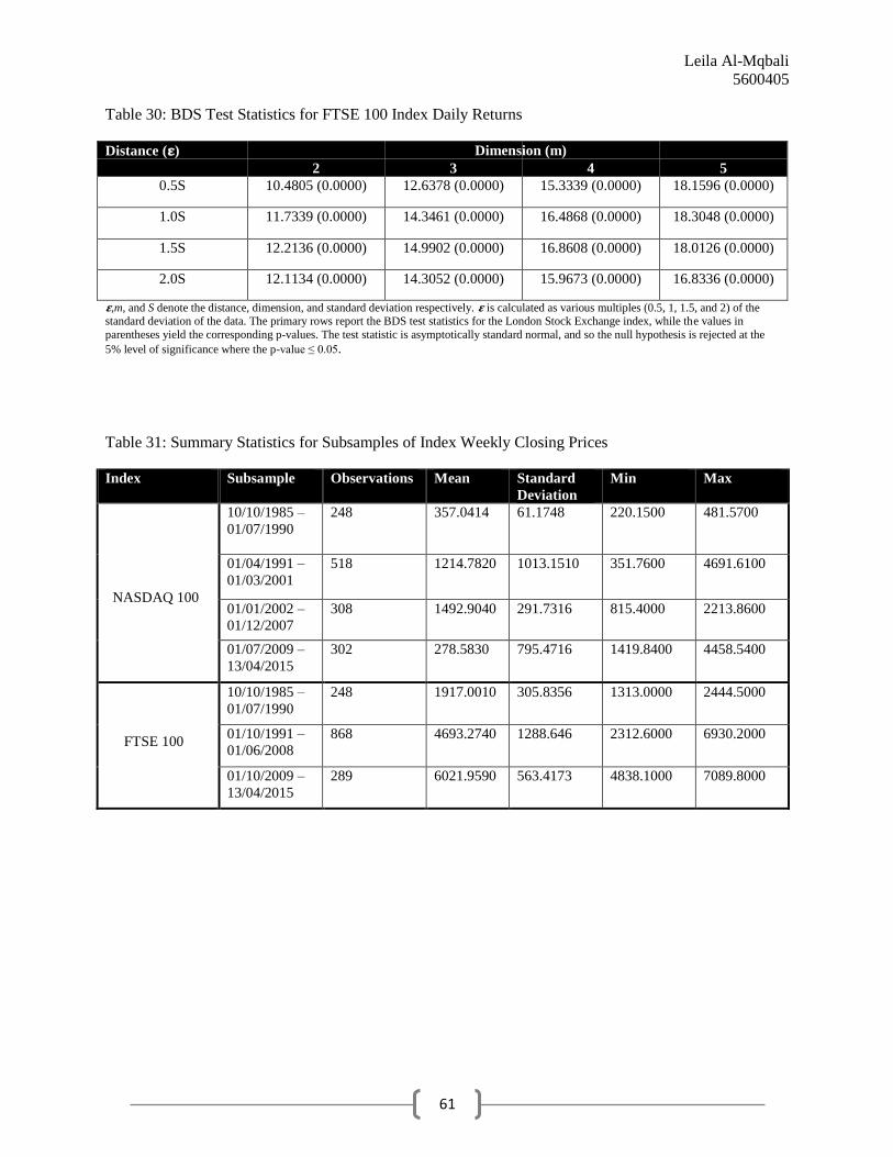
Leila Al-Mqbali

5600405

61

Table 30: BDS Test Statistics for FTSE 100 Index Daily Returns

Distance (𝛆)

2 3 4 5

0.5S 10.4805 (0.0000) 12.6378 (0.0000) 15.3339 (0.0000) 18.1596 (0.0000)

1.0S 11.7339 (0.0000) 14.3461 (0.0000) 16.4868 (0.0000) 18.3048 (0.0000)

1.5S 12.2136 (0.0000) 14.9902 (0.0000) 16.8608 (0.0000) 18.0126 (0.0000)

2.0S 12.1134 (0.0000) 14.3052 (0.0000) 15.9673 (0.0000) 16.8336 (0.0000)

𝛆,m, and S denote the distance, dimension, and standard deviation respectively. 𝛆 is calculated as various multiples (0.5, 1, 1.5, and 2) of the standard deviation of the data. The primary rows report the BDS test statistics for the London Stock Exchange index, while the values in

parentheses yield the corresponding p-values. The test statistic is asymptotically standard normal, and so the null hypothesis is rejected at the

5% level of significance where the p-value ≤ 0.05.

Table 31: Summary Statistics for Subsamples of Index Weekly Closing Prices

Index Subsample Observations Mean Standard

Deviation

Min Max

10/10/1985 –

01/07/1990

248 357.0414 61.1748 220.1500 481.5700

01/04/1991 –

01/03/2001

518 1214.7820 1013.1510 351.7600 4691.6100

01/01/2002 –

01/12/2007

308 1492.9040 291.7316 815.4000 2213.8600

01/07/2009 –

13/04/2015

302 278.5830 795.4716 1419.8400 4458.5400

10/10/1985 –

01/07/1990

248 1917.0010 305.8356 1313.0000 2444.5000

01/10/1991 –

01/06/2008

868 4693.2740 1288.646 2312.6000 6930.2000

01/10/2009 –

13/04/2015

289 6021.9590 563.4173 4838.1000 7089.8000

Dimension (m)

NASDAQ 100

FTSE 100

Leila Al-Mqbali

5600405

62

Table 32: Summary Statistics for Subsamples of Index Weekly Returns

Index Subsample Observations Mean Standard

Deviation

Min Max

10/10/1985 –

01/07/1990

247 0.0031 0.0305 – 0.2314 0.1014

01/04/1991 –

01/03/2001

517 0.00238 0.0485 – 0.6770 0.1914

01/01/2002 –

01/12/2007

307 0.0008 0.0300 – 0.1019 0.1091

01/07/2009 –

13/04/2015

301 0.00377 0.0235 – 0.0786 0.0740

10/10/1985 –

01/07/1990

247 0.0024 0.0268 – 0.2486 0.0486

01/10/1991 –

01/06/2008

867 0.0010 0.0205 – 0.0887 0.0795

01/10/2009 –

13/04/2015

288 0.0011 0.0212 – 0.1028 0.0724

NASDAQ 100

FTSE 100

Leila Al-Mqbali

5600405

63

Table 33: DF-GLS Tests for Subsamples of NASDAQ 100 Weekly Closing Prices

Sub-Period

Number

of Lags

DF-GLS Test

Statistic for

Weekly

Prices

1%

Critical

Value

5%

Critical

Value

10%

Critical

Value

10/10/1985 –

01/07/1990

15 –2.522 –3.480 –2.804 –2.525

8 –2.464 –3.480 –2.868 –2.584

4 –2.413 –3.480 –2.898 –2.612

2 –2.431 –3.480 –2.912 –2.624

1 –2.321 –3.480 –2.918 –2.629

01/04/1991 –

01/03/2001

18 –2.026 –3.480 –2.820 –2.537

16 –1.824 –3.480 –2.828 –2.544

15 –1.946 –3.480 –2.831 –2.547

8 –1.413 –3.480 –2.855 –2.569

4

2

1

–1.347

–1.382

–1.370

–3.480

–3.480

–3.480

–2.867

–2.873

–2.876

–2.580

–2.585

–2.588

01/01/2002 –

01/12/2007

15 –1.337 –3.480 –2.816 –2.536

10 –1.200 –3.480 –2.851 –2.568

8 –1.045 –3.480 –2.864 –2.579

4 –1.006 –3.480 –2.887 –2.600

2 –1.006 –3.480 –2.897 –2.609

1 –1.088 –3.480 –2.902 –2.613

01/07/2009 –

13/04/2015

15 –1.470 –3.480 –2.816 –2.535

9 –1.613 –3.480 –2.858 –2.574

8 –1.787 –3.480 –2.864 –2.580

4 –2.076 –3.480 –2.888 –2.601

2 –2.173 –3.480 –2.898 –2.610

1 –2.296 –3.480 –2.903 –2.615

First Subsample:Maximum lag for the index is 15, selected by the Schwert Criterion. The Ng-Perron criterion alsoselects 15 as the optimal lag,

while the SC criterion and MAIC criterion both choose 1 lag as optimal. Second Subsample:Maximum lag for the index is 18, selected by the Schwert Criterion. The Ng-Perron criterion selects 15 as the optimal lag,

while the SC criterion and MAIC criterion choose 1 and 16 respectively.

Third Subsample:Maximum lag for the index is 15, selected by the Schwert Criterion. The Ng-Perron criterion selects 10 as the optimal lag, while the SC criterion and MAIC criterion both choose 1 lag as optimal.

Fourth Subsample:Maximum lag for the index is 15, selected by the Schwert Criterion. The Ng-Perron criterion selects 8 as the optimal lag,

while the SC criterion and MAIC criterion choose 1 and 9 respectively. Note: The null hypothesis is rejected at the α% level of significance wherever the DF-GLS test statistic ≤ α% critical value. Values marked with

*, **, and *** denote significance at the 10%, 5%, and 1% levels respectively.

Leila Al-Mqbali

5600405

64

Table 34: DF-GLS Tests for Subsamples of NASDAQ 100 Weekly Returns

Sub-Period

Number

of Lags

DF-GLS Test

Statistic for

Weekly Returns

1%

Critical

Value

5%

Critical

Value

10%

Critical

Value

V

10/10/1985 –

01/07/1990

15 –3.781 *** –3.480 –2.804 –2.525

8 –5.161 *** –3.480 –2.868 –2.584

5 –5.148 *** –3.480 –2.892 –2.605

4 –6.465 *** –3.480 –2.898 –2.612

2 –8.659 *** –3.480 –2.912 –2.624

1 –10.028 *** –3.480 –2.918 –2.629

01/04/1991 –

01/03/2001

18 –3.118 ** –3.480 –2.820 –2.537

17 –3.169 ** –3.480 –2.824 –2.541

10 –4.397 *** –3.480 –2.849 –2.563

8 –5.606 *** –3.480 –2.855 –2.569

4

2

1

–8.035 ***

–11.405 ***

–14.567 ***

–3.480

–3.480

–3.480

–2.867

–2.873

–2.876

–2.580

–2.585

–2.588

01/01/2002 –

01/12/2007

15 –1.197 –3.480 –2.816 –2.536

11 –1.309 –3.480 –2.845 –2.562

9 –1.536 –3.480 –2.858 –2.574

8 –1.936 –3.480 –2.864 –2.579

4 –3.563 *** –3.480 –2.887 –2.600

2 –5.886 *** –3.480 –2.897 –2.609

1 –7.685 *** –3.480 –2.902 –2.613

01/07/2009 –

13/04/2015

15 –1.834 –3.480 –2.816 –2.535

13 –1.848 –3.480 –2.830 –2.549

8 –2.031 –3.480 –2.864 –2.580

7 –2.062 –3.480 –2.871 –2.585

4 –2.942 ** –3.480 –2.888 –2.601

2 –4.049 *** –3.480 –2.898 –2.610

1 –5.586 *** –3.480 –2.903 –2.615

First Subsample:Maximum lag for the index is 15, selected by the Schwert Criterion. The Ng-Perron criterion selects 5 as the optimal lag, while the SC criterion and MAIC criterion choose 1 and 5 respectively.

Second Subsample:Maximum lag for the index is 18, selected by the Schwert Criterion. The Ng-Perron criterion selects 10 as the optimal lag, while the SC criterion and MAIC criterion choose 1 and 17 respectively.

Third Subsample:Maximum lag for the index is 15, selected by the Schwert Criterion. The Ng-Perron criterion selects 11 as the optimal lag,

while the SC criterion and MAIC criterion choose 9 and 11 respectively. Fourth Subsample:Maximum lag for the index is 15, selected by the Schwert Criterion. The Ng-Perron criterion selects 13 as the optimal lag,

while the SC criterion and MAIC criterion choose 7 and 13 respectively.

Note: The null hypothesis is rejected at the α% level of significance wherever the DF-GLS test statistic ≤ α% critical value. Values marked with *, **, and *** denote significance at the 10%, 5%, and 1% levels respectively.

Leila Al-Mqbali

5600405

65

Table 35: DF-GLS Tests for Subsamples of FTSE 100 Weekly Closing Prices

Sub-Period

Number

of Lags

DF-GLS Test

Statistic for

Weekly

Prices

1%

Critical

Value

5%

Critical

Value

10%

Critical

Value

10/10/1985 –

01/07/1990

15 –2.054 –3.480 –2.804 –2.525

13 –2.248 –3.480 –2.824 –2.564

8 –1.839 –3.480 –2.868 –2.584

4 –2.400 –3.480 –2.899 –2.612

2 –2.619 –3.480 –2.912 –2.624

1 –2.034 –3.480 –2.918 –2.629

01/10/1991 –

01/06/2008

20 –1.246 –3.480 –2.826 –2.542

8 –1.300 –3.480 –2.849 –2.562

7 –1.292 –3.480 –2.851 –2.564

4 –1.424 –3.480 –2.856 –2.568

2 –1.492 –3.480 –2.859 –2.571

1 –1.466 –3.480 –2.860 –2.572

01/10/2007 –

13/04/2015

15 –2.958 ** –3.480 –2.813 –2.533

13 –2.700 * –3.480 –2.829 –2.548

8 –2.909 ** –3.480 –2.865 –2.581

6 –2.637 * –3.480 –2.878 –2.592

4 –3.035 ** –3.480 –2.890 –2.603

2 –3.647 *** –3.480 –2.901 –2.613

1 –3.524 *** –3.480 –2.906 –2.618

First Subsample:Maximum lag for the index is 15, selected by the Schwert Criterion. The Ng-Perron criterion selects 13 as the optimal lag,

while the SC criterion and MAIC criterion choose 2 and 1 respectively. Second Subsample:Maximum lag for the index is 18, selected by the Schwert Criterion. The Ng-Perron criterion selects 7 as the optimal lag,

while the SC criterion and MAIC criterion both choose 1 lag as optimal.

Third Subsample:Maximum lag for the index is 15, selected by the Schwert Criterion. The Ng-Perron criterion selects 13 as the optimal lag, while the SC criterion and MAIC criterion choose 1 and 6 respectively.

Note: The null hypothesis is rejected at the α% level of significance wherever the DF-GLS test statistic ≤ α% critical value. Values marked with

*, **, and *** denote significance at the 10%, 5%, and 1% levels respectively.

Leila Al-Mqbali

5600405

66

Table 36: DF-GLS Tests for Subsamples of FTSE 100 Weekly Returns

Sub-Period

Number

of Lags

DF-GLS Test

Statistic for

Weekly Returns

1%

Critical

Value

5%

Critical

Value

10%

Critical

Value

10/10/1985 –

01/07/1990

15 –3.607 *** –3.480 –2.804 –2.525

12 –3.974 *** –3.480 –2.833 –2.552

8 –5.728 *** –3.480 –2.868 –2.584

4 –6.720 *** –3.480 –2.899 –2.612

2 –8.133 *** –3.480 –2.912 –2.624

1 –7.980 *** –3.480 –2.918 –2.629

01/10/1991 –

01/06/2008

20 –3.307 ** –3.480 –2.826 –2.542

8 –6.581 *** –3.480 –2.849 –2.562

4 –10.032 *** –3.480 –2.856 –2.568

2 –14.154 *** –3.480 –2.859 –2.571

1 –17.589 *** –3.480 –2.860 –2.572

01/10/2007 –

13/04/2015

15 –3.767 *** –3.480 –2.813 –2.533

9 –5.931 *** –3.480 –2.858 –2.575

8

4

–5.513 *** –3.480 –2.865 –2.581

–8.911 *** –3.480 –2.890 –2.603

2 –9.925 *** –3.480 –2.901 –2.613

1 –11.819 *** –3.480 –2.906 –2.618

First Subsample:Maximum lag for the index is 15, selected by the Schwert Criterion. The Ng-Perron criterion selects 12 as the optimal lag,

while the SC criterion and MAIC criterion both choose 1 as the optimal lag length.

Second Subsample:Maximum lag for the index is 20, selected by the Schwert Criterion. The Ng-Perron criterion also selects 20 as the optimal lag, while the SC criterion and MAIC criterion choose 1 and 20 respectively.

Third Subsample:Maximum lag for the index is 15, selected by the Schwert Criterion. The Ng-Perron criterion selects 9 as the optimal lag,

while the SC criterion and MAIC criterion both choose 1 as the optimal lag length. Note: The null hypothesis is rejected at the α% level of significance wherever the DF-GLS test statistic ≤ α% critical value. Values marked with

*, **, and *** denote significance at the 10%, 5%, and 1% levels respectively.

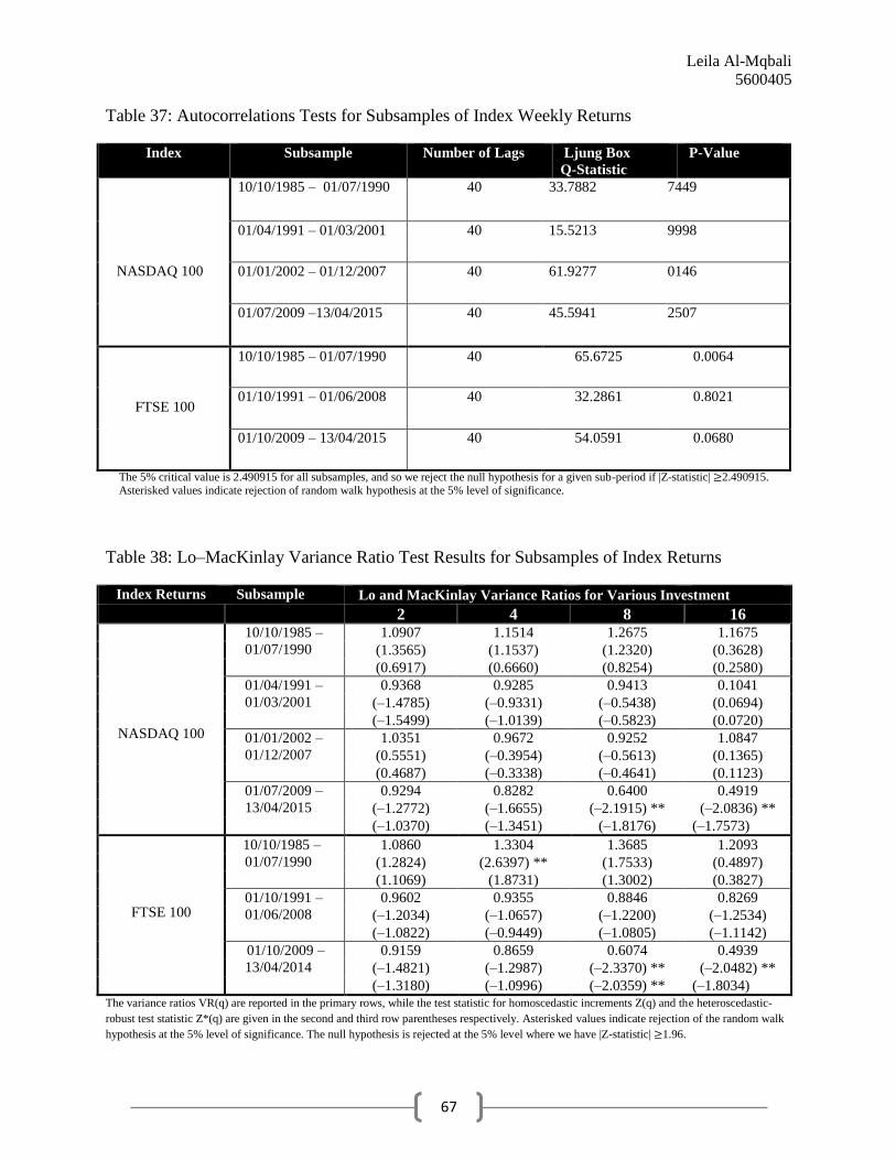
Leila Al-Mqbali

5600405

67

The 5% critical value is 2.490915 for all subsamples, and so we reject the null hypothesis for a given sub-period if |Z-statistic| ≥2.490915. Asterisked values indicate rejection of random walk hypothesis at the 5% level of significance.

Table 37: Autocorrelations Tests for Subsamples of Index Weekly Returns

Index Subsample Number of Lags Ljung Box

Q-Statistic

P-Value

NASDAQ 100

10/10/1985 – 01/07/1990

40 33.7882 0.7449

01/04/1991 – 01/03/2001 40 15.5213 0.9998

01/01/2002 – 01/12/2007 40 61.9277 0.0146

01/07/2009 –13/04/2015 40 45.5941 0.2507

FTSE 100

10/10/1985 – 01/07/1990 40 65.6725 0.0064

01/10/1991 – 01/06/2008 40 32.2861 0.8021

01/10/2009 – 13/04/2015 40 54.0591 0.0680

Table 38: Lo–MacKinlay Variance Ratio Test Results for Subsamples of Index Returns

Index Returns Subsample

2 4 8 16

NASDAQ 100

10/10/1985 –

01/07/1990

1.0907 1.1514 1.2675 1.1675

(1.3565) (1.1537) (1.2320) (0.3628)

(0.6917) (0.6660) (0.8254) (0.2580)

01/04/1991 –

01/03/2001

0.9368 0.9285 0.9413 0.1041

(–1.4785) (–0.9331) (–0.5438) (0.0694)

(–1.5499) (–1.0139) (–0.5823) (0.0720)

01/01/2002 –

01/12/2007

1.0351 0.9672 0.9252 1.0847

(0.5551) (–0.3954) (–0.5613) (0.1365)

(0.4687) (–0.3338) (–0.4641) (0.1123)

01/07/2009 –

13/04/2015

0.9294 0.8282 0.6400 0.4919

(–1.2772) (–1.6655) (–2.1915) ** (–2.0836) **

(–1.0370) (–1.3451) (–1.8176) (–1.7573)

FTSE 100

10/10/1985 –

01/07/1990

1.0860 1.3304 1.3685 1.2093

(1.2824) (2.6397) ** (1.7533) (0.4897)

(1.1069) (1.8731) (1.3002) (0.3827)

01/10/1991 –

01/06/2008

0.9602 0.9355 0.8846 0.8269

(–1.2034) (–1.0657) (–1.2200) (–1.2534)

(–1.0822) (–0.9449) (–1.0805) (–1.1142)

01/10/2009 –

13/04/2014

0.9159 0.8659 0.6074 0.4939

(–1.4821) (–1.2987) (–2.3370) ** (–2.0482) **

(–1.3180) (–1.0996) (–2.0359) ** (–1.8034) The variance ratios VR(q) are reported in the primary rows, while the test statistic for homoscedastic increments Z(q) and the heteroscedastic-

robust test statistic Z*(q) are given in the second and third row parentheses respectively. Asterisked values indicate rejection of the random walk

hypothesis at the 5% level of significance. The null hypothesis is rejected at the 5% level where we have |Z-statistic| ≥1.96.

Lo and MacKinlay Variance Ratios for Various Investment

Horizons

Leila Al-Mqbali

5600405

68

Table 39: Chow and Denning Multiple Variance Ratio Test Results for Index Returns

Index Returns Subsample Homoscedastic

Statistic

Heteroscedastic

Statistic

10/10/1985 – 01/07/1990 1.356487 0.825363

01/04/1991 –01/03/2001 1.478549 1.549895

01/01/2002 –01/12/2007 0.561320 0.468738

01/07/2009 – 13/04/2015 2.191476 1.817578

FTSE 100

10/10/1985 – 01/07/1990 2.639678 ** 1.873051

01/10/1991 – 01/06/2008 1.253416 1.114228

01/10/2009 – 13/04/2014 2.336798 2.035850

The 5% critical value is 2.490915, and so we reject the null hypothesis if |Z-statistic| ≥ 2.490915. Asterisked values indicate rejection of random

walk hypothesis at the 5% level of significance.

Table 40: Runs Tests Results for Subsamples of Index Returns

Index

Returns

Subsample Residuals

≤ 0

Residuals

> 0

Expected

Runs

Actual

Runs

Z-Score Prob>|z|

NASDAQ

100

10/10/1985 –

01/07/1990

108 138 122 123 0.11 0.91

01/04/1991 –

01/03/2001

234 282 257 251 –0.51 0.61

01/01/2002 –

01/12/2007

151 155 154 169 1.72 0.09

01/07/2009 –

13/04/2015

141 159 150 150 –0.05 0.96

FTSE 100

10/10/1985 –

01/07/1990

112 134 123 130 0.9 0.37

01/10/1991 –

01/06/2008

419 447 434 449 1.05 0.29

01/10/2009 –

13/04/2015

127 160 143 134 –1.03 0.30

The null hypothesis rejected at the 5% level of significance if | Z-score | ≥ 1.96.

NASDAQ 100

Leila Al-Mqbali

5600405

69

2

3

4

5

10/10/1985 –

01/07/1990

0.5S 0.7257 (0.4680) 1.9997 (0.0455) 2.0301 (0.0423) 2.1249 (0.0336)

1.0S 1.7131 (0.0867) 2.0562 (0.0398) 1.9497 (0.0512) 2.1972 (0.0280)

1.5S 2.7754 (0.0055) 3.0516 (0.0023) 2.6724 (0.0075) 2.7970 (0.0052)

2.0S 3.7647 (0.0002) 4.1279 (0.0000) 3.7006 (0.0002) 3.6379 (0.0003)

01/04/1991 –

01/03/2001

0.5S 4.5357 (0.0000) 5.4719 (0.0000) 6.9807 (0.0000) 8.0579 (0.0000)

1.0S 5.3445 (0.0000) 6.0723 (0.0000) 7.3543 (0.0000) 8.1521 (0.0000)

1.5S 5.1041 (0.0000) 5.6989 (0.0000) 6.7289 (0.0000) 7.5043 (0.0000)

2.0S 4.1201 (0.0000) 4.3982 (0.0000) 4.9606 (0.0000) 5.4110 (0.0000)

01/01/2002 –

01/12/2007

0.5S 2.6759 (0.0075) 2.6917 (0.0071) 3.5164 (0.0004) 4.7490 (0.0000)

1.0S 2.3441 (0.0191) 2.7774 (0.0055) 3.6665 (0.0002) 4.6434 (0.0000)

1.5S 2.2586 (0.0239) 3.2636 (0.0011) 4.5099 (0.0000) 5.5888 (0.0000)

2.0S 2.4180 (0.0156) 3.1023 (0.0019) 4.3694 (0.0000) 5.2671 (0.0000)

01/07/2009 –

13/04/2015

0.5S 3.6859 (0.0002) 5.4257 (0.0000) 6.7282 (0.0000) 7.5065 (0.0000)

1.0S 3.9908 (0.0001) 5.7569 (0.0000) 7.1660 (0.0000) 7.9423 (0.0000)

1.5S 4.7211 (0.0000) 6.1501 (0.0000) 7.0267 (0.0000) 7.3304 (0.0000)

2.0S 4.9434 (0.0000) 6.2638 (0.0000) 6.9320 (0.0000) 7.1018 (0.0000)

Index Returns Subsample Distance(𝛆) Dimension (m)

Table 41: BDS Test Results for Subsamples of NASDAQ 100 Index Returns

NASDAQ 100

𝛆,m, and S denote the distance, dimension, and standard deviation respectively. 𝛆 is calculated as various multiples (0.5, 1, 1.5, and 2) of the standard deviation of the data. The primary rows report the BDS test statistics for the London Stock Exchange index, while the values in parentheses yield the corresponding p-values. The test statistic is asymptotically standard normal, and

so the null hypothesis is rejected at the 5% level of significance where the p-value ≤ 0.05. Values in red denote the only cases where the null hypothesis cannot be rejected.

Leila Al-Mqbali

5600405

70

2

3

4

5

10/10/1985 –

01/07/1990

0.5S 1.7281 (0.0840) 2.8229 (0.0048) 2.4404 (0.0147) 2.5460 (0.0109)

1.0S 1.9338 (0.0532) 3.1271 (0.0018) 2.9894 (0.0028) 3.1931 (0.0014)

1.5S 1.5888 (0.1121) 3.1523 (0.0016) 3.1535 (0.0016) 3.4201 (0.0006)

2.0S 1.2641 (1.2062) 3.2510 (0.0011) 3.4338 (0.0006) 3.6566 (0.0003)

01/10/1991 –

01/06/2008

0.5S 2.9889 (0.0028) 5.3936 (0.0000) 6.6522 (0.0000) 8.1650 (0.0000)

1.0S 3.5371 (0.0004) 5.9344 (0.0000) 7.0460 (0.0000) 8.4203 (0.0000)

1.5S 3.5021 (0.0005) 5.6403 (0.0000) 6.4599 (0.0000) 7.5549 (0.0000)

2.0S 2.8742 (0.0041) 4.8027 (0.0000) 5.3056 (0.0000) 6.1974 (0.0000)

01/10/2009 –

13/04/2015

0.5S 1.9812 (0.0476) 3.2973 (0.0010) 5.8644 (0.0000) 6.7610 (0.0000)

1.0S 2.4377 (0.0148) 3.9855 (0.0001) 4.8892 (0.0000) 4.8820 (0.0000)

1.5S 1.9980 (0.0457) 3.5678 (0.0004) 4.2053 (0.0000) 4.2145 (0.0000)

2.0S 1.8448 (0.0651) 3.2545 (0.0011) 3.7172 (0.0002) 3.7314 (0.0002)

Index Returns Subsample Distance(𝛆) Dimension (m)

𝛆,m, and S denote the distance, dimension, and standard deviation respectively. 𝛆 is calculated as various multiples (0.5, 1, 1.5, and 2) of the standard deviation of the data. The primary rows report the BDS test statistics for the London Stock Exchange index, while the values in parentheses yield the corresponding p-values. The test statistic is asymptotically standard normal, and so the null hypothesis is rejected at the 5% level of significance where the p-value ≤ 0.05. Values in red denote the only cases where the null hypothesis cannot be rejected.

FTSE 100

Table 42: BDS Test Results for Subsamples of FTSE 100 Index Returns

Returns