Edith Cowan University Edith Cowan University

Research Online Research Online

Theses: Doctorates and Masters Theses

1-1-1999

An empirical comparison using both the term structure of interest An empirical comparison using both the term structure of interest

rates and alternative models in pricing options on 90-day BAB rates and alternative models in pricing options on 90-day BAB

futures futures

Irene Chau Edith Cowan University

Follow this and additional works at: https://ro.ecu.edu.au/theses

Part of the Finance and Financial Management Commons

Recommended Citation Recommended Citation Chau, I. (1999). An empirical comparison using both the term structure of interest rates and alternative models in pricing options on 90-day BAB futures. https://ro.ecu.edu.au/theses/1207

This Thesis is posted at Research Online. https://ro.ecu.edu.au/theses/1207

Edith Cowan UniversityResearch Online

Theses: Doctorates and Masters Theses

1999

An empirical comparison using both the termstructure of interest rates and alternative models inpricing options on 90-day BAB futuresIrene ChauEdith Cowan University

This Thesis is posted at Research Online.http://ro.ecu.edu.au/theses/1207

Recommended CitationChau, I. (1999). An empirical comparison using both the term structure of interest rates and alternative models in pricing options on 90-dayBAB futures. Retrieved from http://ro.ecu.edu.au/theses/1207

Edith Cowan University  

 

Copyright Warning      

You may print or download ONE copy of this document for the purpose 

of your own research or study.  

The University does not authorize you to copy, communicate or 

otherwise make available electronically to any other person any 

copyright material contained on this site.  

You are reminded of the following:  

Copyright owners are entitled to take legal action against persons who infringe their copyright. 

 

A reproduction of material that is protected by copyright may be a 

copyright infringement. Where the reproduction of such material is 

done without attribution of authorship, with false attribution of 

authorship or the authorship is treated in a derogatory manner, 

this may be a breach of the author’s moral rights contained in Part 

IX of the Copyright Act 1968 (Cth). 

 

Courts have the power to impose a wide range of civil and criminal 

sanctions for infringement of copyright, infringement of moral 

rights and other offences under the Copyright Act 1968 (Cth). 

Higher penalties may apply, and higher damages may be awarded, 

for offences and infringements involving the conversion of material 

into digital or electronic form.

USE OF THESIS

The Use of Thesis statement is not included in this version of the thesis.

AN EMPIRICAL COMPARISION USING BOTH THE TERM STRUCTURE

OF INTEREST RATES AND ALTERNATIVE MODELS

IN PRICING OPTIONS ON 90-DA Y BAB FUTURES

Irene Chao Master of Business (Finance) Unit Controller : Dave ADen Edith Cowan University

ABSTRACT

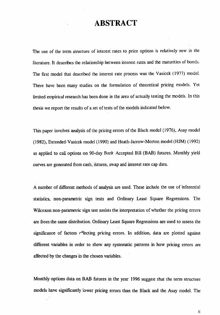
The use of the term structure of interest rates to price options is relatively new in the

literature. It describes the relationship between interest rates and the maturities of bonds.

The first model that described the interest rate process was the Va'iicek (1977) model.

There have been many studies on the formulation of theoretical pricing models. Yet

limited empirical research has been done in the area of actually testing the models. In this

thesis we report the results of a set of tests of the models indicated below.

This paper involves analysis of the pricing errors of the Black model ( 1976), Asay model

(1982), Extended-Vasicek model ( 1990) and Heath-Jarrow-Morton model (HJM) ( 1992)

as applied to call options on 90-day Ban.k Accepted Bill (BAB) futures. Monthly yield

curves are generated from cash, futures, swap and interest rate cap data.

A number of different methods of analysis are used. These include the use of inferential

statistics, non-parametric sign tests and Ordinary Least Square Regressions. The

Wilcoxon non-parametric sign test assists the interpretation of whether the pricing errors

are from the same distribution. Ordinary Least Square Regressions are used to assess the

significance of factors r-~ecting pricing errors. In addition, data are plotted against

different variables in order to show any systematic patterns in how pricing errors are

affected by the changes in the chosen variables.

Monthly options data on BAB futures in the year 1996 suggest that the term structure

models have significantly lower pricing errors than the Black and the Asay model. The

ii

Heath-Jarrow-Morton model (1992) is overall the hettcr model to usc. For the term

structure models, pricing errors show a decreasing trend as moncyness increases. The

EXtended-Vasicek model and the HJM model have significantly lower errors for deep in­

the-money and out-of-the-money options. Higher mean absolute errors arc observed for

at-the-money options for both term structure models. The HJM model overprices at-the­

money options but underprices in and out-of-the-money options while the Extcndcd­

Vasicek model underprices deep-in-the-money options but overprices options of other

categories.

The mean and absolute etTors for both the Black model and the Asay model rise as time

to maturity and volatility increac;es. The two models overprice in, at and out-of-the­

money options and the mean pricing error is lowest for in-the-money options.

The results suggest that the factor time to maturity is significant at the 0.05 level to the

-mean pricing error for all four models. Moneyness is the only insignificant factor when

the Asay model is used. It is also negatively correlated to mean pricing error for the

Black model, the Asay model, the Extended-Vasicek model and the HJM model. The R­

square for the Extended-Vasicek model was found to be the lowest. Overall, the HJM

model gives the lowest pricing error when pricing options on 90-Day Bank Accepted Bill

Futures.

iii

"I certify that this thesis docs not incorporate without acknowledgement any material

previously submitted for a degree or diploma in any institution of higher education; and

that to the best of my knowledge and belief it does not contain any material previously

published or written by another person except where due references is made in the text."

Signatu~ Date: ____ ~:3""D._,/34/'-'<f..J.C( __

iv

ACKNOWLEDGEMENT

I wish to acknowledge my thanks to my superviSor, Dave Allen, for making useful

comments and for assisting in the data collection procedure and the running of the Monis

Software.

I owe due thanks to my family, especially my mum and dad, and my grandma, who have

supported me mentally throughout my five years at university. I also want to thank my

friend, Steven Seow, for his support and assistance.

Irene Chau

Mar, 1999.

v

TABLE OF CONTENTS

TITLE PAGE

USE OF THESIS

ABSTRACT

DECLARATION

ACKNOWLEDGEMENTS

TABLE OF CONTENTS

Chapter I: INTRODUCTION

1.1 BACKGROUND OF THE STUDY

II

IV

v

vii

1.1.1 TERM STRUCTURE OF INTEREST RATES 2

1.2 THESIS OUTLINE 4

Chapter 2: REVIEW OF THE LITERATURE

2.1 BLACK MODEL 6

2.2 ASAYMODEL 10

2.3 SPECIHC TERMS IN TERM STRUCTURE II

2.4 THE EXPECTATIONS HYPOTHESIS IS

2.4.1 RISK NEUTRAL PRICING 16

2.5 THE TERM STRUCTURE THEORY 18

2.5.1 ASSUMPTIONS 18

2.5.2 VALUING INTEREST RATE DERIVATIVE

SECURITIES 20

vii

2.6 REVIEW OF MODELS 22

2.6.1 ONE FACTOR MODELS 22

2.6.1.1 Vasicek Model (1977) 22

2.6.1.2 Cox-Ingersoll-Ross Model (ClR) .( 1985) 25

2.6.1.3 Empirical research on the use of one-factor

models 27

2.6.2 MODEL PROCESSES 28

2.6.2.1 The State Space Process 28

2.6.2.2 The Bond Price Process 28

2.6.2.3 The Forward Rate Process 28

2.6.3 TWO-FACTOR MODELS 29

2.6.3.1 Brennan-Schwartz Model ( 1979) 29

2.6.3.2 Chen and Scott (1992) 30

2.6.3.3 Longstaff-Schwartz Model ( 1993) 31

2.6.3.4 Chan, Karolyi, Longstaff and Sanders (1992) 32

2.6.3.5 Empirical Research on the use of

Two-Factor Models 33

2.6.4 MULTIFACTOR MODELS 34

2.6.4.1 Chen (1996) 34

2.6.5 FORWARD RATE MODELS 35

2.6.5.1 Ho and Lee Model ( 1986) 36

2.6.5.2 Hull and White Model (1990) 39

2.6.5.3 Heath-larrow-Morton Model(HJM) ( 1992) 42

viii

2.7 NEW DIRECTIONS

2.8 IMPLICATIONS

Chapter 3: METHODOLOGY

3.1 DESIGN

3.2 INSTRUMENT

3.3 PARAMETER ESTIMATION

3.3.1 BLACK MODEL

3.3.1.1 Time to Maturity

3.3.1.2 Volatility

3.3.2 ASAYMODEL

3.3.3 THE TERM STRUCTURE MODELS

3.3.3.1 The Yield Curve, the Extended-Vasicek

Volatility, the HJM Volatility and the

Reversion Rates

3.4 DATA PROCESSING PROCEDURE

3.4.1 BLACK MODEL AND ASA Y MODEL

3.4.2 THE TERM STRUCTURE MODELS

3.5 DATAANALYS1S

3.5.1 SPSS

3.5.2 GRAPHICAL ANALYSIS

3.5.3 WILCOXON SIGNED RANKS TESTS

3.5.4 OLS REGRESSION AND WHITE'S

ADJUSTMENTS

46

48

49

51

53

53

53

53

55

57

57

58

58

58

68

68

69

69

70

I

ix

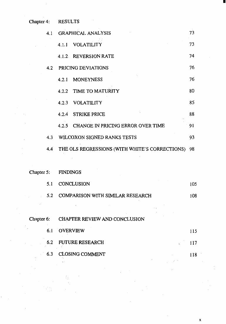
Chapter 4: RESULTS

4.1 GRAPHICAL ANALYSIS

4.1.1 VOLATILITY

4.1.2 REVERSION RATE

4.2 PRICING DEVIATIONS

4.2.I MONEYNESS

4.2.2 TIME TO MATURITY

4.2.3 VOLATILITY

4.2.4 STRIKE PRICE

4.2.5 CHANGE IN PRICING ERROR OVER TIME

4.3 WILCOXON SIGNED RANKS TESTS

4.4 THE OLS REGRESSIONS (WITH WHITE'S CORRECTIONS)

Chapter 5: FINDINGS

5.1 CONCLUSION

5.2 COMPARISON WITH SIMILAR RESEARCH

Chapter 6: CHAPTER REVIEW AND CONCLUSION

6.1 OVERVIEW

5.2 FUTURE RESEARCH

6.3 CLOSING COMMENT

73

73

74

76

76

80

85

88

9I

93

98

105

108

115

117

118

I

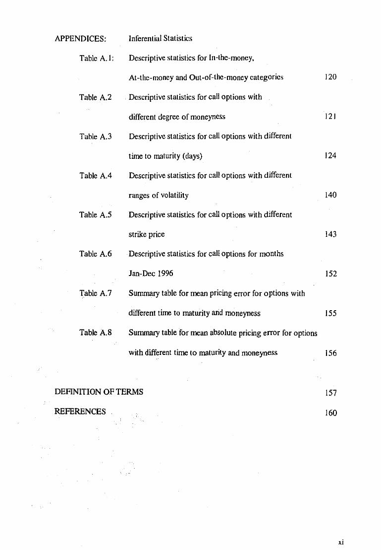
APPENDICES: Inferential Statistics

Table A.l: Descriptive statistics for In-the-money,

At-the-money and Out-of-the-money categories

Table A.2 Descriptive statistics for call options with

different degree of moneyness

Table A.3 Descriptive statistics for call options with different

time to maturity (days)

Table A.4 Descriptive statistics for call options with different

ranges of volatility

Table A.5 Descriptive statistic!; for call options with different

strike price

Table A.6 Descriptive statistics for call options for months

Jan-Dec 1996

Table A.7 Summary table for mean pricing error for options with

different time to maturity and rnoneyness

Table A.8 Sununary table for mean absolute pricing error for options

with different time to maturity and moneyness

DEFINITION OF TERMS

REFERENCES

120

121

124

140

143

152

155

156

157

160

xi

Chapter 1: INTRODUCTION

1.1 BACKGROUND TO THE STUDY

Empirical analysis of option prices has concentrated on two distinct questions. The first

is concerned with discriminating between alternative pricing models. The second area of

concern deal'i with the accuracy with which market participants estimate the parameters

needed to implement the option pricing formulas. The present study is within the first

category, and is aimed specifically at testing the efficiency of aJternative models in

pricing options on bond futures. The purpose of the study is to apply two term structure

models: the Extended-Vasicek model and the Heath-Jarrow-Morton model, to the

pricing of call options on 90-day bank accepted bill futures options. Theoretical prices

will be used to compare with actual settlement prices to determine the accuracy of the

models. Any systematic discrepancies are analyzed. The prices obtained from the two

term structure models are also compared to the Black (1976) model and the Asay (1982)

Model in order to determine the effect on pricing.

The most widely used model in option pricing is the Black-Scholes Option Pricing model

(1973). Black aod Scholes were the first to derive ao aoalytic solution for the price of a

European option on a non-dividend paying stock. The value of the option was

determined by arbitrage considerations rather than by an investor's risk preferences

about the future performance of the stock. The value of an option depends on ( 1) the

stock price, (2) the exercise price of the option, (3) the volatility of the stock's return,

(4) the time to maturity, and (5) the continuously compounded short-term interest rate

for borrowing aod lending. They assumed that the stock's returns foUowed a normal

I

distribution. The model assumes that the distribution of security prices is skewed, so that

higher prices arc more likely to occur than lower prices.

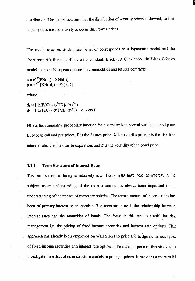
The model assumes stock price behavior corresponds to a lognormal model and the

short-term risk-free rate of interest is constant. Black ( 1976) extended the Black-Scholcs

model to cover European options on commodities and futures contracts:

c = e'T[FN(dt)- XN(d,)] p = e'T [XN(-d,)- FN(-d,)]

where

d1 = [ ln(F/X) + dT/2j/ (<TiT) d2 = [ ln(F/X)- <iT/2]/ (CJ'iT) = d1 -<TiT

N(.) is the cumulative probability function for a standardized normal variable, c and pare

European call and put prices, F is the fulures price, X is the strike price, r is the risk-free

interest rate, T is the time to expiration, and cr is the volatility of the bond price.

1.1.1 Tenn Structure oflnterest Rates

The term structure theory is relatively new. Economists have held an interest in the

subject, as an understanding of the term structure has always been important to an

understanding of the impact of monetary policies. The tenn structure of interest rates has

been of primary interest to economists. The term structure is the relationship between

interest rates and the maturities of bonds. The f0cus in this area is useful for risk

management i.e. the pricing of fixed income securities and interest rate options. This

approach has already been employed on Wall Street to price and hedge numerous types

of fixed-income securities and interest rate options. The main purpose of this study is to

investigate the effect of term structure models in pricing options. It provides a more valid

2

guide to the pricing of interest rate-contingent claim<.; in an Australian context. To price

interest rate derivatives, the evolution of the entire yield curve must he modelled.

The uses of the term structure arc as follows:

( 1) Analyze the returns for asset commitments of different termc;. Portfolios can be

varied according to the quality, coupon level, time to maturity and the type of issuer.

The tenn structure allows investors to make judgements about the short-term

rewards of different maturity strategies as interest rates change.

(2) Assess the expectation of future interest rates. Analysis of the term structure allows

the interpretation of the expectation of future interest rates.

(3) Price bonds and other fixed-payment contracts. The yield curves give an expectation

of the alternative yields for coupon-bearing bonds. Some bonds and contracts are

priced in such a way that the yield would be equal to the yield at the same maturity

on the yield curve with the adjustment for credit quality or other important factors.

The pricing errors can be minimized for zero coupon bonds and other fmancial

instruments with non-traditional cash-flow patterns. The separation of pricing of cash

flows with different term structures can increase the accuracy of pricing.

(4) Pricing contingent claims on flxed income securities. The use of the tenn structure of

interest rates to price options is relatively new in the literature. It describes the

relationship between interest rates and the maturities of bonds. Yield curve models

describe the probabilistic behaviour of the yield curve over time. They deal with

movements in a whole yield curve - not changes to a single variable. As time passes,

the individual interest rates in the term structure change causing the shape of the

curve to change.

3

I

The Black model docs not include any of the underlying term structure information when

applied to options on imcrcst rate instruments. Asay ( 1982) modiJics the Black Model

and allows for the application of the nmrking-to-markct position for options on futures

as is the case in the Australian market.

It has been suggested that there arc four approaches in the literature to the valuation of

interest rate options. The frrst follows Black and Scholes and uses the price of the

underlying bond as an exogenous variable. The second models the endogenous term

structure of interest rates in a no-arbitrage framework. These include the Vasicek ( 1977)

model and Brennan and Schwartz (1979, 1982). The term structure model developed for

pricing in Cox, Ingersoll and Ross (1985) represents an equilibrium specification that is

completely consistent with stochastic production and with changing investment

opportunities. The third approach, pioneered by Ho and Lee (1986) and Heath, Jarrow,

and Morton ( 1990, 1992) begins with the evolution of the entire zero coupon price

curve. The fourth approach, as suggested by Black, Derman, and Toy (i 990) and Hull

and White (1990, 1993), specifies the spot rate process and detertnines the model in such

a way that the model is consistent with the current term structure. There have been many

studies on the formulation of theoretical pricing models but limited empirical research

has been done in this area particularly as applied to the no-arbitrage models. Buhler,

Uhrig, Walter and Weber (1995) provide one of the few empirical comparisons of some

of these models.

1.2 THESIS OUTLINE

This dissertation is divided into six sections. The frrst chapter is the introduction; it

justifies the research and it gives a brief summary of the purpose and scope of the study.

4

The contribution of the term structure of interest rates in the financial services industries

is also discussed. Chapter two provides a literature review in term-; of general and

specific literature in the area of term structure of interest rates, assumptions and an

overview of the different pricing models. Some definitions of specific tcrrno; arc also

given. Chapter three presents the research methodology. Results arc presented in chapter

four which examines how the pricing errors are affected by the factors Hke time to

maturity, moneyness and volatility. Comparisons are made between the Black model, the

Asay model, the Extended Vasicek model and the Heath-Jarrow-Morton model. Chapter

five summarizes the fmdings. The significance of the study can be assessed. This is

followed by suggestions for future research.

5

Chapter 2: REVIEW OF THE LITERATURE

An outline of the Black model was given in chapter one. This chapter elaborates on the

different tests and hypothesis being put forward. How the term structure of interest rates

was introduced in application to option pricing will be discussed. The chapter form"i a

basis of understanding for the alternative models used for pricing in this study.

2.1 Black Model

After the introduction of the Black model, it was challenged by different researchers.

They looked into the possibility of alternative distributional hypotheses.

Galai (1983) summarizes the empirical approaches to validating option-pricing models.

There are a few methodologies within which the models can be tested. The first approach

is by means of simulations and quasi-simulations of deviations from the basic

assumptions of the models. The sensitivity of the model prices to empirical deviations

from the assumptions is tested. Bhattacharya (1980) tests the actual distribution of stock

prices rather than the assumed lognormal distribution.

The other approaches in testing the models involve comparisons of the model prices to

actual prices. The estimated parameters of the model and the actual observations of

stock prices are placed in the pricing model to generate expected option prices. The

model pricos are compared to the actual, realized option prices. The tests have the ability

to show whether model prices are unbiased estimators of actual prices and whether there

are consistent deviations that can be exploited for better prediction or for making above­

normal profits. The third approach in testing the models involves imputing the standard

6

deviations from actual option prices by usmg a pricing model. It assumes that all

parameters arc known and that markets arc efficient and synchronous. The standard

deviation can be imputed as the only unknown in the equation when equating the actual

price to the model price. The Iaiit approach is based on creating neutral hedge positions

and testing the behavior of the returns from the investment. This should create a riskless

position for options and their underlying stock when the model is correct. In this case,

the problem of risk-adjustment for investment in options is eliminated and returns on the

hedge position should equal the risk~ free rate.

In his summary of the tests put forward by different studies, Galai (!983) concludes that

the B!ack-Scholes model performs relatively well, especially for at-the-money options.

No alternative model consistently offers better prediction of market prices than the

Black-Scholes model. Also, for short time periods, the Black-Scholes model gives good

predictions of market prices for options that are undervalued and overvalued. The Black­

Scholes model assumes constant variance. There has been a great deal of work

examining alternative diffusion processes. There is some evidence in favour of the

constant elasticity of variance model, but this is inconclusive. Nonstationarity of the risk

estimator of the underlying stock is a major problem that affects the perfonnance of the

Black-Scholes model. The evidence does not seem to support the null hypothesis of

market synchronization. The tests of the boundary conditions suggest that trading

synchronization or data synchronization are important considerations.

The other approach in testing the consistency between options and time series is by

estimating model · parameters implicit in option prices and testing the distributional

predictions for the underlying time series. This is usually done by two procedures: (I) the

7

parameters inferred from option prices arc assumed known with certainty. (2) their

informarional content is tested using time series data. In order to (est the time-series

distributions, option prices must satisfy certain no-arbitrage constraints. Firstly, option

prices relative to the synchronous underlying asset price cannot be below intrinsic value

and European call and put prices of common strike price must satisfy put-call parity.

Also, American and European option prices, with respect to strike price, must be

equivalent to the risk-neutral distribution function being non-decreasing. The risk-neutral

probability must be non-negative. Evnine and Rudd (1985) and Bhattacharya (1983) find

that option prices tend to violate lower bound constraints. Bhattacharya (1983) examines

CBOE American options on 58 stocks over the period 1976-1977 to find that 1.3% of

the options tested violate the immediate-exercise lower bound and 2.38% violate the

European intrinsic value lower bound.

Ogden and Tucker (1987) examined pound, Deutschemark and Swiss franc call and put

options and found only 0.8% violate intrinsic-value bounds. Consistent with Ogden and

Tucker ( 1987), Bates found around 1% of the Deutschemark call and put transaction

prices over 1984-1991 violate intrinsic value bounds computed from futures prices.

Violations which are generally less than estimated transaction costs suggests that the

violations may originate in imperfect synchronization between the options market and the

underlying asset market or in bid-ask spreads.

The literature on ARCH and GARCH models addresses the issue of estimating

conditional variance when volatility is time-varying. Bates ( 1996) provides a brief survey

of work in this area. Melino and TumbuU ( 1990) fmd that the stochastic volatility model

8

docs reduce pricing errors. Further confirrrwtory evidence is provided by Cao ( 1992),

and Myers and Hanson (1993).

Besides the Black-Schnles Option Pricing model, other models that were proposed in

pricing interest rate contingent claims include the jump diffusion model and the constant

elasticity of variance mode~. Merton (1976) introduced a jump-diffusion model under

the assumption of diversifiable jump risk and independent lognormally distributed jumps.

He suggested that distributions with fatter tails than the lognormal model might explain

the tendency for deep-in-the-money, deep-out-of-the money, and short-maturity options

to sell for more than their Black-Scholes value, and the tendency of near-the-money and

longer-maturity options to sell for less. Cox and Ross (1976b) proposed pricing models

for European options under absolute diffusion, pure jump, and square root constant

elasticity of variance models of the return on the underlying asset. Option pricing models

under stochastic volatility were put forward by Hull and White ( 1987). The main issue of

concern is whether option prices are consistent with the time series properties of the

underlying asset price. Hypotheses tested include cross-sectional tests of whether high­

volatility stocks tend to have high priced options. Bates (1996) summarizes the various

theoretical implications behind different models tested. Other tests examine whether

volatility inferred from option prices using the Black-Scholes model is an unbiased and

efficient predictor of future volatility of the underlying asset price. The other important

problem relates to non-constant variance which is the focus of the previously mentioned

ARCWGARCH time series estimation procedures. This questions whether the tenn

structure of volatilities inferred from options of different maturities is consistent with

predictable changes in volatilities.

9

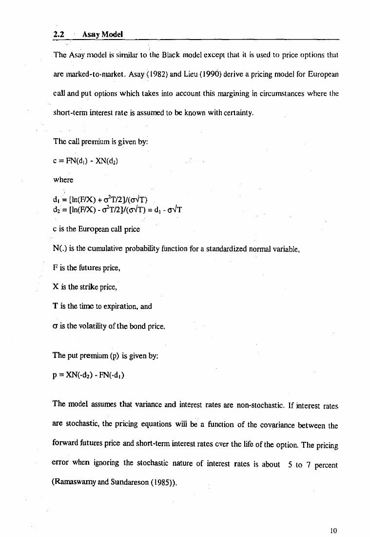
2.2 Asay Model

The Asay model is similar to the Black model except that it is used to price options that

are marked-to-market. Asay ( 1982) and Lieu (1990) derive a pricing model for European

call and put options which takes into account this margining in circum'itances where the

short-term interest rate is assumed to be known with certainty.

The call premium is given by:

c = FN(d,) - XN(d,)

where

' d1 = [ln(F/X) + crT/2]/(cr-iT) d, = [ln(F/X)- crT/2]/(cr-iT) = d1 - cr-JT

c is the European call price

N(.) is the cumulative probability function for a standardized normal variable,

F is the futures price,

X is the strike price,

T is the time to expiration, and

cr is the volatility of the bond price.

The put premium (p) is given by:

p = XN(-d,)- FN(-d,)

The model assumes that variance and interest rates are non-stochastic. If interest rates

are stochastic, the pricing equations will be n function of the covariance between the

forward futures price and short-term interest rates ever the life of the option. The pricing

error when ignoring the stochastic nature of interest rates is about 5 to 7 percent

(Ramaswamy and Sundareson (1985)).

10

Brace and Hodgson ( 1991) use the Asay model to compare different estimates of

historical volatility. Actual standard deviation was regressed on both historical and

implied standard deviations. It was concluded that no one measure of historical volatility

was consistent with observed market price. The price sensitivity in the Black and Ar.;ay

model pricing equations are highly affected by volatility estimates. Empirical analysis ha'i

tended to focus on issues related to volatility (Brown and Shevlin ( 1983 ), Hull and White

( 1987)).

Options on futures in the Sydney Futures Exchanges have futures style margining. The

contracts are marked to market at the end of each day. Brown and Taylor (1997)

examined the Asay model on transaction prices from the SPI futures option market for

the period from I June 1993 through to 30 June 1994. They found that the errors arc

related to the degree of moneyness and the maturity of the option. The model generates

significant pricing errors which are consistent with an observed •smile' in the implied

volatilities.

2.3 SPECIFIC TERMS IN TERM STRUCTURE

Spot Rates

A spot interest rate is the rate applying to money borrowed now, to be repaid at some

future date. Money can be borrowed for various lengths of time and theretbre there will

be a range of spot rates at any moment in time, each rate relating to the period of the

borrowing. The relationship between these interest rates and the term of the borrowing is

known as the term structure of interest rates. If P(O,l) is the price of a one-year zero

coupon bond and P(0,2) is the price of a two-year zero-coupon bond. Using the term

structure of interest rates, the price of a one-year bond with one dollar face value will be

II

P(O,l) = 1/(1 + r(O,l)). The two-year bond price will be P(0,2) = 1/(1 + r(0,2)) etc.

Therefore, spot rates r(O,l), r(0,2), ... , r(O,T) make up the term structure going out T

periods. They represent transactions as bonds undertaken on the spot.

Forward Rate

The forward rate is a rate in which one can contract at time 0 to borrow or lend at a

future date. If F(O, I ,2) is the rate that can be locked in today for a bond that would be

issued in one year and matures in 2 years. The bond would have a one-year maturity and

its price can be specified as F(O,l,2). By the end of two years, for every dollar invested,

the total amount of [l/P(O,l)][l/F(O,l,2)] can be gained. This should be equal to the

return per dollar from buying a two-year bond today and holding it for two years i.e.

l/P(0,2). If F(O,I,2) ¢ P(0,2)/P(O,l), an arbitrage profit can be earned. Therefore, any

forward price F(O,i,j) = P(O,j)/P(O,i).

Since F(O,I,2) = P(0,2)/P(O,l) and that F(0,2,3) = P(0,3)/P(0,2); combining the two

relationships, F(0,2,3) = P(0,3)/[ P(O,l) F(0,1,2)] or P(O,l) F(O,l,2) F(0,2,3) = F(0,3).

Thus, the price of a three-period bond today is the product of the price of a one-period

bond and the forward price of a one-period bond starting at time I and another one­

period bond starting at time 2.

Example : The yield on the two year bond (7.53% per annum) can be replicated by

buying a one year bond now (yielding 7.24%) and a one-year-to-maturity bond in one

year's time.

(I + R,)'

(1.0753)2

=(I +R,) (I+ 1R,)

= (1.0724) (I+ 1R,)

12

(l+,R1) = ( 1.0753)2 I ( 1.0724)

= 1.0782 (7.82%)

1R1 is known as the implied forward rate - the interest rate implied by the current term

structure for one-year borrowing in one year's time. Similar calculations can indicate the

implied forward rate for a bond of any term at any future point in time covered by the

term structure.

A one-year rate in two years' time (2R1) is given by:

(I + R,)'

(1.0765)3

=(I+ R2)2 (I+ ,R,)

=(1.0753)2 (1 + 2R1)

= (1.0765)3/ (1.0753)2

= 1.0789

2R1 = 0.0789 (7.89%)

The yield on the three one-year borrowing equals the current yield on a three-year bond:

(I+ R,)3 =[(I+ R,) (I+ ,R,) (I+ 2R1)]10

= [ 1.0724 X 1.0782 X 1.0789]18

= 1.0765 (7.65% as per the term structure data)

Overall, the series will be raised to the power of 1/N where N is the number of years

involved.

Arbitrage V s No-arbitrage Models

No-arbitrage models take the term structure as an input whilst arbitrage models produce

the term structure as an output. Since market prices do not confonn to these model

prices, this creates the possibility of arbitrage even when the volatility parameter of the

13

model used L'i fairly accurate. No-arbitrage models take the current price of the asset as

given and derive a model that relates to the evolution of the term structure.

Some examples of these approaches arc shown below:

lahk I I ,,\111\)h·-. 11\ \dtill,l~l' aml \u-;n•hilla~l' \lmhl, · · · '

Arbitrage Models Vasicek (1977) Cox, Ingersoll and Ross ( 1985)

No-arbitrage Models Ho and Lee ( 1985) Extended-Vasicek ( 1989) Heath, !arrow and Morton (1992)

The arbitrage-free binomial model is based on a lattice of interest rates. The yields on the

lattice represent a series of possible future short-term interest rates formed to satisfy

conditions preventing changes in the yield curve that allow arbitrage opportunities. Cox

and Ross (1976a) explained that the no-arbitrage constraints reflect the fundamental

properties of the risk-neutral distribution implicit in options prices. The no-arbitrage

constraints are respectively : (I) call and put option prices relative to the synchronous

underlying asset price cannot be below intrinsic value and American option prices cannot

be below European prices. (2) American and European option prices must be monotone

and convex functions of the underlying strike price. (3) synchronous European call and

put prices of common strike price and maturity must satist)' the put-call parity.

If the no-arbitrage constraints are violated, there is no distributional hypothesis

consistent with observed option prices. Studies that use more carefully synchronized

transactions data have found that substantial proportions of option prices violate lower

bound constraints (Bhattacharya ( 1983), Evnine and Rudd ( 1985)). Violations of

intrinsic value constraints are observed for short-maturity, in-the-money and deep-in-the-

money options, as outlined in Section 2.1. Interest rate based derivative securities have

14

structures that are much more complicated compared with those of derivatives on stocks.

This makes it difficult to value the contracts analytically. The evolution of the entire yield

curve has to be known. The price of interest rate derivatives is the value of the expected

discounted future cash flow, with the assumption of risk-neutral expectations. This ili

similar to the Black and Scholes model for stock option prices. However, when

contingent clairm based on interest rate sensitive securities are being priced, interest rates

change over time. The discount rate is usually correlated with the cash-flow of the

interest rate contingent claim which further complicates the issue.

2.4 THE EXPECTATIONS HYPOTHESIS

The expectations theory holds in a world of certainty or risk neutral borrowers and

lenders. Investors are not assumed to be risk neutral but rather when hedging a derivative

with the underlying asset, arbitrage possibilities can and will be exploited by all investors

regardless of which way prices go because of the assumption of full information.

According to the pure expectations theory, forward rates exclusively represent the

expected future rates. Therefore, the entire term structure at a given time reflects the

market's current expectation of the future short rates. To clearly explain the forward

rates, assume a discount bond that matures in period four. rl, r2, r3 and r4 are short-

tenn interest rates in periods one, two, three and four.

If the short-term rate moves as follows:

A $1 face value discount bond should then be priced at:

P= I (I +rl)( I +r2)( I +r3)( l+r4)

15

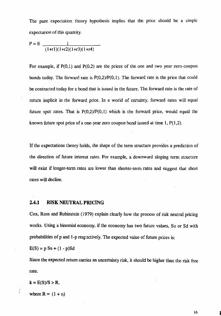
The pure expectation theory hypothesis implies that the price should he a simple

expectation of this quantity.

( l+rl)( l+r2)( l+r3)( 1 +r4)

For example, if P(O,l) and P(0,2) are the prices of the one and two year zero-coupon

bonds today. The forward rate is P(0,2)/P(O, 1 ). The forward rate is the price that could

be contracted today for a bond that is issued in the future. The forward rate is the rate of

return implicit in the forward price. In a world of certainty, forward rates will equal

future spot rates. That is P(0,2)/P(O,l) which is the forward price, would equal the

known future spot price of a one-year zero coupon bond issued at time 1, P( I ,2).

If the expectations theory holds, the shape of the term structure provides a prediction of

the direction of future interest rates. For example, a downward sloping term structure

will exist if longer-tenn rates are lower than shorter-term rates and suggest that short

rates will decline.

2.4.1 RISK NEUTRAL PRICING

Cox, Ross and Rubinstein ( 1979) explain clearly how the process of risk neutral pricing

works. Using a binomial economy, if the economy has two future values, Su or Sd with

probabilities of p and 1-p respctively. The expected value of future prices is:

E(S) = pSu+ (1- p)Sd

Since the expected return carries an uncertainty risk, it should be higher than the risk free

rate.

k = E(S)/S > R,

where R = (1 + rr)

16 I

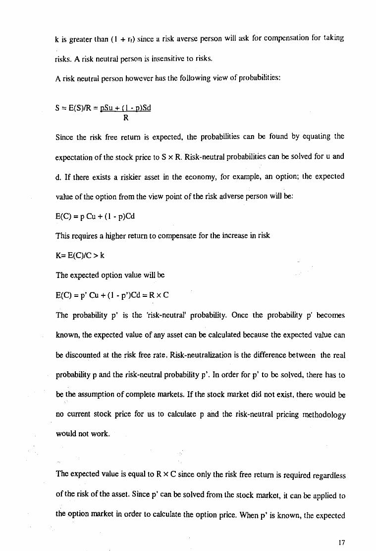
k is greater than (I + rr) since a risk averse person will ask li:>r compensation for taking

risks. A risk neutral person is insensitive to risks.

A risk neutral person however has the following view of probabilities:

S = E(S)/R = pSu +(I- plSd R

Since the risk free return is expected, the probabilities can be found by equating the

expectation of the stock price to S x R. Risk-neutral probabilities can be solved for u and

d. If there exists a riskier asset in the economy, for example, an option: the expected

value of the option from the view point of the risk adverse person will be:

E(C) = p Cu + (1- p)Cd

This requires a higher return to compensate for the increase in risk

K=E(C)/C> k

The expected option value will be

E(C) = p' Cu +(I - p')Cd = R x C

The probability p' is the 'risk-neutral' probability. Once the probability p' becomes

known, the expected value of any asset can be calculated because the expected value can

be discounted at the risk free rate. Risk-neutralization is the difference between the real

probability p and the risk-neutral probability p'. In order for p' to be solved, there has to

be the assumption of complete markets. If the stock market did not exist, there would be

no current stock price for us to calculate p and the risk-neutral pricing methodology

would not work.

The expected value is equal to R x C since only the risk free return is required regardless

of the risk of the asset. Since p' can be solved from the stock market, it can be applied to

the option market in order to calculate the option price. When p' is known, the expected

17

value of any asset can be derived and the value can be found by discounting at the risk

free rate.

In order to price under a tenn structure in a continuous framework, a utility function is

assumed to obtain risk aversion. The risk premium between the actual probability and the

riskMneutral probability can be found. For example, the face value of a $1 bond in a

continuous time setting has the following pricing formula:

P(t,T) = E, [exp(-J,T r(x)dx)]

t and T are the current time and the maturity time of the bond. The expectation is taken

at time t.

If the random movements of future interest rates over time are assumed to follow known

distributions, the bond prices can be computed by using the expected vaiue risk neutral

formula.

2.5 THE TERM STRUCTURE THEORY

2.5.1 Assumptions

The assumptions underlying the use of the term structure in pricing is explained in

Jarrow (1996) and other earlier studies such as Ho and Lee (1986). The economy is

assumed to be frictionless and competitive. The frictionless market's assumptions are

justified since the activities of large institutional traders approximate frictionless markets

as their transaction costs are minimal. All securities are assumed to be infinitely divisible

and the market for any fmancial security is perfectly liquid.

18

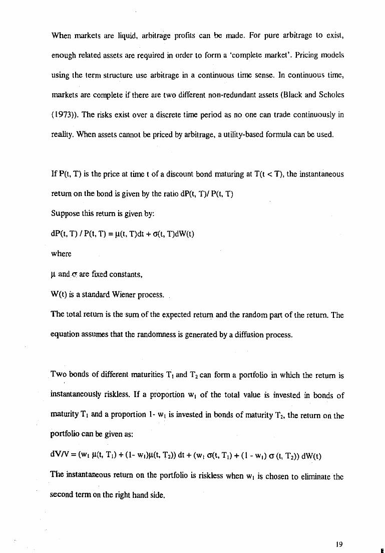
When markets are liquid, arbitrage profits can be made. For pure arbitrage to exist,

enough related assets are required in order to form a 'complete market'. Pricing models

using the term structure use arbitrage in a continuous time sense. In continuous time,

markets are complete if there are two different non-redundant assets (Black and Scholes

( 1973)). The risks exist over a discrete time period as no one can trade continuously in

reality. When assets cannot be priced by arbitrage, a utility-based formula can be used.

If P(t, T) is the price at time t of a discount bond maturing at T(t < T), the instantaneous

return on the bond is given by the ratio dP(t, T)/ P(t, T)

Suppose this return is given by:

dP(t, T) I P(t, T) = 11(t, T)dt + cr(t, T)dW(t)

where

11 and 0' are fixed constants,

W(t) is a standard Wiener process.

The total return is the sum of the expected return and the random part of the return. The

equation assumes that the randollUless is generated by a diffusion process.

Two bonds of different maturities T 1 and T 2 can form a portfolio in which the return is

instantaneously riskless. If a proportion w1 of the total value is invested in bonds of

maturity T1 and a proportion l- w1 is invested in bonds of maturity T2, the return on the

portfolio can be given as:

dVN = (w, 11(1, T,) + (1- w,)l1(t, T,)) dt + (w 1 cr(t, T1) +(I- w1) cr (t, T 2)) dW(t)

The instantaneous return on the portfolio is riskless when w1 is chosen to eliminate the

second term on the right hand side.

t9 I

This instantaneous return has to be equal to the short -term interest rate:

{!l(t, T 1)- rjl cr(t, T 1) = {!l(t, T 1)- rj I cr(t, T,)

The equation says that the expected return in excess of risk-free rate associated with

holding a bond divided by the standard deviation of the return (excess return per unit

risk) is independent of the maturity of the bond. Let A.(r, t) = (!l(t, T) - r)lcr (r,t). A.(r, t) is

the market price of risk.

The return on the bond maturing at T can be shown to be:

dP(t, T) I P(t, T) = (r(t) +a (t, T)A.(r, t)) dt + cr (t, T)dW(t)

The bond price can be obtained as the solution to the boundary condition P(T,T) = I, in

which the price at maturity is equal to I. The models described in the following sections

demonstrate the different approaches used to solve the bond price process.

2.5.2 VALUING INTEREST RATE DERIVATIVE SECURITIES

The stochastic behavior of interest rates is very difficult to model. The various risk-free

interest rates available in the economy can be represented by the term structure. This is

the interest rate earned on a default-free discount bond until its time to maturity. Interest

rates also appear to follow mean-reverting processes. This refers to the drift which pulls

the interest rate back to the long-run average level. Forward interest rates can also be

deduced from the term structure. Early studies assume all the underlying assets'

distributions be lognonnal with known parameters.

Models of the short-term interest rate assume the short rate follows a diffusion process

and the price of the discount bond depends only on the short-term rate over its term

(Attari 1997). The general form of the evolution of the short-term interest rate is

20

nornmlly assumed to be:

dr; u(r, t) dt + p(r, t) dW(t)

where a(r, t) is the 'drift', the instantaneous expected change in the short-term interest

rate; and p(r, t) is the volatility or the random change in the short-term interest rate. The

drift and the volatilit~1 can both be functions of the current level of interest rates.

When the short-term interest rate is assumed to be the only. source of uncertainty in the

model, Ito's Lemma applied to the bond price gives:

dP = P,dt + P,dr + 0.5 P.(dr)2

P is used in place of P(t,T) and the subscripted variables denote partial derivatives.

P, is the partial derivative of the bond price with respect to current time.

Substituting for dr from the general evolution of short-term interest rate equation and

comparing with the return on the bond equation yields:

P, + a(r, t)+ p(r, t)A(r, t))P, + 0.5p(r, t)2 Prr- rP, = 0

This can be solved for P(t, T), the price of the discount bond using the appropriate

boundary equation. The above equation is referred to as the fundamental partial

differential equation for the bond price.

The different types of short-term interest rate models depend on how the market price of

risk A(r, t) is specified. A(r, t) can be treated as a function of short-term interest rater

and current time t. If A(r, t) is chosen to make models analytically tractable, it is

important that economic equilibrium arguments are also considered.

21

The evolution of short-term interest rate models can generally be summarized in the

following equation:

dr = CI(~- r)dt + o' dW(t)

The short-term lnterest rate process should allow for mean reversion. The volatility of

interest rates should al.;;o depend on the level of short-term interest rates.

The following section is a summary of the different types of models that incorporate the

term structure of interest rates. Chen ( 1996) provides the following classifications.

2.6 REVIEW OF MODELS

2.6.1 ONE FACTOR MODELS

Discrete single factor models are models with one source of uncertainty in which only

one of two possibilities can happen (movements in interest rates up or down) at each

node in the tree. In a continuous framework, one factor is solely responsible for the

evolution of L11.terest rates. A model that provides great insights on how the term

structure of interest rate could be modelled is the Vasicek Model.

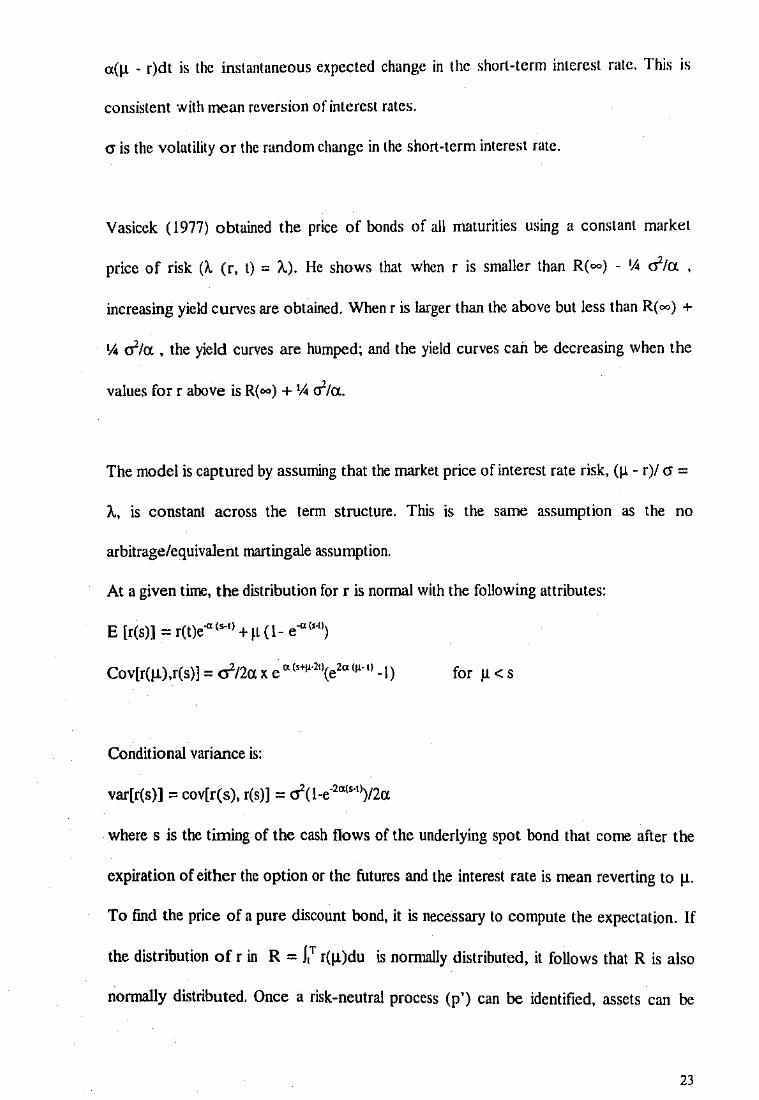
2.6.1.1 Vasicek Model (1977)

Vasicek (1977) modelled the interest rate as a continuous time process. The interest rate

process was:

dr =a(~- r)dt + odW(t)

where a, 11. and o are fixed constants and W(t) is a standard Wiener process,

dr is the change in the spot rate r,

dW can be viewed as normal variate with mean 0 and variance dt '

22

a(~ . r)dt is the instantaneous expected change in the short-term interest rate. This is

consistent with mean reversion of interest rates.

o is the volatility or the random change in the short-term interest rate.

Vasicek (1977) obtained the price of bonds of all maturities using a constant market

price of risk (l. (r, t) = /..). He shows that when r is smaller than R(~) - 'A rita. ,

increasing yield curves are obtained. When r is larger than the above but less than R( oo) +

\4 rita. , the yield curves are humped; and the yield curves can be decreasing when the

values for r above is R(~) + 1A rita..

The model is captured by assuming that the market price of interest rate risk, (~ - r)t cr =

A, is constant across the term structure. This is the same assumption as the no

arbitrage/equivalent martingale assumption.

At a given time, the distribution for r is normal with the following attributes:

E [r(s)] = r(t)e~'~'' + IL (1- e~<•·' 1)

Cov[r(!l).r(s)] = dna. x e "'""'211

(e2" '"''

1 -I) for ~ < s

Conditional variance is:

var[r(s)] = cov[r(s), r(s)] = ri(l-e2"'"'1)t2a.

where s is the timing of the cash flows of the underlying spot bond that come after the

expiration of either the option or the futures and the interest rate is mean reverting to ~·

To find the price of a pure discount bond, it is necessary to compute the expectation. If

the distribution of r in R = ),T r(!l)du is normally distributed, it follows that R is also

normally distributed. Once a risk-neutral process (p') can be identified, assets can be

23

priced using the risk-free return regardless of their actual risks. The risk-neutral mean

and variance arc:

E',[R] = ),TE', [r(s)]ds = r(t)(l-e·•<T-o/ a)+ (1!- (qcr)/u) [T- t- (1-c·•<T-u/ a)]

and V', [R] = V,[R]

The risk-neutral mean is changed by the risk parameter q which is fixed under log utility.

The risk-neutral variance remains unchanged since r is nonnally distributed.

Given the parameters a, J.l , a and q, bond prices for a given maturity can be calculated:

P(t,T) = e-E't<R>+ V't!R)I2 = e·rttJF\t.TJ- G<t.T>

where

F(t,T) = (1- e~<T-o)/u

G(t,T) = (1!- (qcr)/u- cr'l2cr')[T- t- F(t,T)] + [cr'F2(t,T)]/4ct

Since interest rates are normally distributed, it is possible for the interest rate to become

negative. Taking the limit ·or the expected rate and variance when T 4 oo shows that as

long as a > 0, the expectation will converge to band the variance will converge to ri'/2

a.

While the Vasicek (1977) model is arbitrage-free in the sense that no bond or options

prices produced by the model will permit arbitrage, it is not arbitrage-free in the context

of actual market prices. This is due to the fact that the model produces a term structure

as an output but does not accept the term structure as an input. Another limitation of the

Vasicek ( 1977) model is that it carmot capture the more complex term structure shifts

24

that occur since it is only a single factor model. Moreover, all rates have the same

volatility.

There is no known solution for American options so the Vasicek model must be laid out

in a binomial or trinomial tree. Hull and White ( 1989) modify the Vasicek model by using

the trinomial tree to solve the problem of fitting the current term structure.

Dothan ( 1978) models the interest rate process as an exponential random walk with no

drift:

dr = rcrdt

This is obtained by setting a = 0 and "( = I. In this case the short-term interest rates

cannot become negative.

2.6.1.2 Cox·lngersoU-Ross Model (CIR) (1985)

Cox, IngersoU, and Ross ( 1985) develop a one factor model and propose an economy

driven by a number of processes that affect the rate of return to assets including

technological change or an inflation factor. The short-term interest rate process in Cox,

JngersoU, and Ross (1985) is assumed to be:

dr= a(J.l· r)dt + crlr dt

where a, ll and 0' are fixed constants,

dr is the change in the spot rate r,

a(J.L- r)dt is the instantaneous expected change in the short-term interest rates,

This is consistent with the mean reversion of interest rates.

25

cr is the volatility or the random change in the shorHerm interest rate. A square root

process for the evolution of interest rate is used.

They show the bond price solution to be:

P, + « (~- r)P,- l.rP, + 1/2 cr' r Prr- r P = 0

This is a model similar to Vasicek's but overcomes the problem of negative interest rates.

If the interest rate can be negative, bond prices can exceed one. When the current rate

moves to zero, the square root of zero causes the volatility to go to zero and the rate will

be pulled up by its drift. To ensure that the short-term rate does not become 0, CIR

assume that 2«~ <! cr'.

The boundary behaviour of the short-rate process does not need to be specified when the

process does not allow the short rate to reach infinity. This model assumes the diffusion

process has a square root ofr. All future interest rates are non-negative.

The analytical solution for the term structure in the CIR model is:

P,(t) =A, (t) exp(-B1 (t)r,)

where

(Cox eta!. (p. 393))

A, (t) = [21iexp((o + y)tl2) I (o + y) (exp(Ot)- I)+ 2o] 2"'"'

B, (t) = [2(exp(Oy)- 1) I (0 + y) (exp(Ot)- 1) + 20] and o = (y + 2cr')'"

Converting to a yield

r, (t) = [-log (A1 (t)) + B1 (t)r,JI t

The level of the term structure depends on the value of r, at any point in time while the

slope of the curve depends upon the variables of the diffusion equation and the market

26 I

price of risk. One deficiency of their model, however, IS that it will never exactly

reproduce an observed yield curve.

Arbitrage models such as Vasicek (1977) and Cox-Ingersoll-Ross (1985) value all

interest rate derivatives on a common basis. Nevertheless, the model's term structure

does not correctly price actual bonds. These models have too few parameters to be

adjusted and they do not take the initial term structure into account. They may aUow

negative interest rates (Vasicek (1977)) or assume perfect correlation between volatility

and the short rate (Cox-Ingersoll-Ross (1985)). The short rate is not sufficient to explain

the future yield curve changes.

2.6.1.3 Empirical Research on the use of One-Factor Models

Brown and Dybvig (1986) test the parameters of the CIR model and compute the

residuals defmed by the gap between the observed bond prices and the predictions of the

model. Residuals show specification errors present in the model.

From the evidence obtained, it seems unreasonable to assume that the entire money

market is given by only one explanatory variable. Moreover, it is hard to obtain a realistic

volatility structure for the forward rates without introducing a very complicated short

rate model. These considerations have led authors to propose models that use more than

one state variable.

27

2.6.2 MODEL PROCESSES

2.6.2.1 The State Space Proces.•

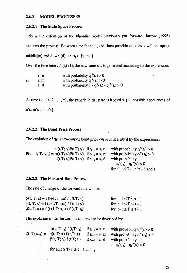
This is the extension of the binomial model previously put forward. Jarrow (1996)

explains the process. Between time 0 and l, the three possible outcomes will he: up(u),

middle(m) and down (d); i.e. s1 E [u,m,d]

Over the time interval [t,t+ I], the new state s1+t is generated according to the expression:

s, u Sttt = s1 m

s, d

with probability q,"(s,) > 0 with probability q, "(s,) > 0 with probability l - q,"(s,) - q,"(s,) > 0

At timet E (1, 2, ... , t}, the generic initial state is laheled ~ {all possible t sequences of

u's, m's and d's).

2.6.2.2 The Bond Price Process

The evolution of the zero-coupon bond price curve is described by the expressions:

u(t,T; s,)P(t,T; ~) if~.,=~ u P(t + I, T; s,.1) = m(t,T; s.)P(t,T; ~) if s,.1 = s, m

d(t,T; ~)P(t,T; ~) if s,., = ~ d

2.6.2.3 The Forward Rate Process

The rate of change of the forward rate will he:

a(t, T; ~) = f (t+ I ,T; s,u) If (t,T; s,) 1(t, T; ~) = f (t+ l,T; s,m) If (t,T; s,)

P(t, T; ~) = f (t+l ,T; ~d) If (t,T; ~)

with probability q,"(~) > 0 with probability q,"(s.) > 0 with probability I - q,"(~) - q,"(s,) > 0 forallt,;T-1 ,;t-1 ands

for t+ I 5 T ,; t- I for t+l ,;T,; t- I for t+l ,;T ,;,_I

The evolution of the forward rate curve can he described by:

a(t, T; s,) f (t,T; s,) f(t, T; ~") = 1(t, T; s,) f (t,T; s,)

PCt, T; s,) f (t,T; s,)

if St+i = s, U

ifs,+t = s, m if St+l = Sc d

forallt,;T-1 ,;,_, ands,

with probability q,"(s,) > 0 with probability q,"(s,) > 0 with probability l - q,"(s,) - q,"(~) > 0

28

The spot rate process evolution is described as:

u (t + I, t + 2; s, u ) r(t+ l,s,.1)= m(t+ l,t+2;s, m)

d (t + I, t + 2; s, d )

with probability q,"(s,) > 0 with prvhability q,m(s1) > 0 with probability I - q,u(s,) - q/n(s,) > 0

Longstaff (1989) develops a 'double square-root' process which makes the term

structure fit more accurately compared to the CIR model. The interest rate process is:

dr = a(6 - Vr)dt + crlr dt

His model allows the short-term rate to be zero in which 2a11 < d is possible. The

possibility of the short-term rate being zero allows the model to fit the current term-

structure better.

Chen (l996b) describes in detail the use of Brerman-Schwartz (1979), Richard model

(1978) and Longstaff-Schwartz (1993) model.

2.6.3 TWO-FACTOR MODELS

2.6.3.1 Brennan-Schwartz Model (1979)

Brerman and Schwartz (1979) use short and long rates as factors, which are the two ends

of tbe yield curve. The short and long rate follows a jump diffusion lognormal process

and the short rate displays mean reversion to the long rate.

dIn r = a(ln l-In r)dt + b1dW1

d I= I a(r, I, b,)dt + b, I dW2

where

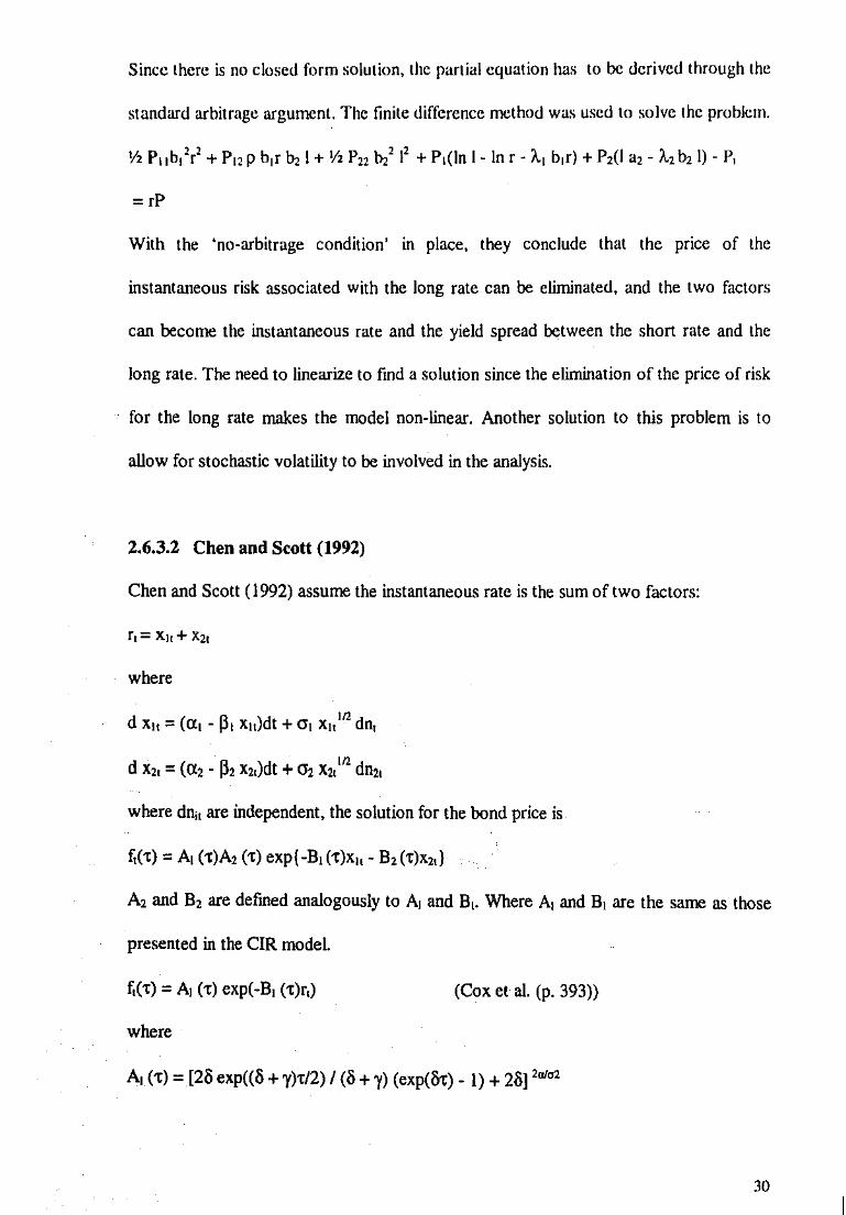
Since there is no closed form solution, the partial equation has to be derived through the

standard arbitrage argument. The finite difference method was used to solve the problem.

y, P11 b12r2 + P12 p b1r b, I+ y, P22 b,2 12 + P,(ln 1- In r- 1.1 b,r) + P,(l a,- f., b,l)- P,

=rP

With the 'no-arbitrage condition' in place, they conclude that the price of the

instantaneous risk associated with the long rate can be eliminated, and the two factors

can become the instantaneous rate and the yield spread between the short rate and the

long rate. The need to linearize to fmd a solution since the elimination of the price of risk

for the long rate makes the model non-linear. Another solution to this problem is to

allow for stochastic volatility to be involved in the analysis.

2.6.3.2 Chen and Scott (1992)

Chen and Scott (1992) assume the instantaneous rate is the sum of two factors:

where

d x,, =(a, - ~~ Xtt)dt +a, Xtt 112 dn1

d x, = (a2 - ~' x,,)dt + cr2 x2,'n dn2,

where dnit are independent, the solution for the bond price is

f,(') =A, (')A,(') exp{ -B, (')x,- B,(,)x,.)

A, and B, are defmed analogously to A, and B1• Where A1 and B1 are the same as those

presented in the CIR model.

f,(,) =A,(') exp(-B1 (')r,)

where

(Cox et a!. (p. 393))

A,(')= [20 exp((O + y),/2) I (o + y) (exp(M)- I)+ 20] >ala>

30

B,(t)=[2(cxp(liy)-l)/(o+y)(cxp(&t)-1)+2o] ando=(y+2cr'J'n

The equation allows the inclusion of any number of factors as long as they arc assumed

to be independent.

2.6.3.3 Longstaff·Schwartz Model (1993)

In Longstaff-Schwanz (1993) model, two factors are also used. They are the short-term

interest rate and the volatility of the short-term rate. They retain the rest of the

assumptions of the CIR model. Factors are observable and parameters can be directly

estimated from the data. Maximum likrJihood estimation is possible since the process

assumption is imposed direc~ly on factors. Longstaff and Schwartz write the two state

variables as:

d y1 =(a- b y,)dt + d y,dW,

d y2 = (k- e y,)dt + 'fV y,dW, where dW, dW, = 0

The equilibrium rate of interest and its volatility are:

2 n' v = (J. y, + p y,

The two factors are related to the underlying rate of return process rather than directly to

the instantaneous rate as in Chen and Scott (1992). The second factor they use affects

only the conditional variance of the rate of return process but both factors affect the

conditional mean. P(O, 0, t, T) < 14 implies that the forward rates are strictly positive.

As the short-term rate increases, the price of the bond can either increase or decrease, for

small values of T-t bond values decrease but for larger values of T-t, bond values may

either decrease or increase. This is due to the fact that an increase in the short -term

interest rate, while keeping the volatility constant, implies a lower production uncertainty

31

and a lower A. This is an important factor that makes this model diftCr from the other

models considered. Changes in volatility and the interest rate constant will have an effect

on the shape and the slope of the term structure. r ~o evidence is found in support of the

rejection of the Longstaff and Schwartz two-factor model, whilst similar tests reject the

one-factor CIR model.

In Chen and Scott (1992), two factors are regarded as driving the short-term rate and its

conditional volatility. The nominal instantaneous interest rate is the sum of the two

components. They both affect the mean and variance. However, more research has to be

done to know how well the models can replicate the unconditional standard deviations of

yield changes.

2.6.3.4 Chan, Karolyi, Longstaff and Sanders (1992)

Chan, Karoyl, Longstaff and Sanders (1992) compared the various short-tenn riskless

rate using the Generalized Method of Moments. They frnd that the most successful

models in capturing the dynamics of the short-term interest rates are those that allow the

volatility of interest rate changes to be highly sensitive to the level of the riskless rate.

The equation that represents the interest rate process is:

dr =(a+ Pr)dt + m1 dz

To estimate the parameters of the above equation, the discrete time specification

equation is given as:

32

Various short-term rate specifications with different parameter restrictions arc then

evaluated against each other. Only weak evidence of mean reversion (p is not

significantly ditTerent from 0) is found. The models explain 1-3 per cent of the variation

in rand they explain up to 20 per cent of the variation in volatility.

Of the most frequently used models the Vasicek (1977) model perform' poorly relative

to the less known models (Dothan ( 1978) and Cox, Ingersoll and Ross (1985)). It was

conunonly known that interest rate volatility is important in valuing contingent claims

and hedging interest rate risk. However, these models fail to capture the dependence of

the term structure's volatility on the·level of interest rate.

2.6.3.5 Empirical Research on the use of Two-Factor Models

Single factor models are useful for clarifying the mathematical concepts involved but are

not useful for applications. They imply that zero-coupon bonds of different maturities are

perfectly correlated, which is not true. Therefore, more factors can be added to the term

structure models in order to improve pricing. The two-factor model has been used in a

framework which either assumes arbitrage-free conditions or is based on utility equations

(Richard (1978), Brennan and Schwartz (1979), Langetieg (1980), Cox, Ingersoll, and

Ross (1985) and Longstaff and Schwartz (1992)). Cox, Ingersoll, and Ross (1985) fmd

that the instantaneous rate can be expressed by separate factors in equilibrium. One

method of modelling is to decompose the instantaneous rate into two factors following

two stochastic processes. The other way is to view the volatility of the instantaneous

interest rate as a function of two factors. The process then follows a single stochastic

volatility model. Chen and Scott ( 1993) fmd the parameters of the model by maximum

likelihood estimation and provide some evidence that at least two factors are required to

]]

I

capture the term structure adequately. Other studies using the generalized method of

moments (Heston (1989), Gibbons and Ramaswamy (1993)) and factor analysis also

found this to be true. This suggests the need for an increased number of factors in the

models.

2.6.4 MULTIFACTOR MODELS

The extension from a one-factor model to a two-factor model corresponds to adding an

additional branch on every node in the appropriate tree. The procedure for extending the

model to a multifactor framework is similar in the process of evolution.

The need for fitting the yield curve suggested tests for multiple factors. Factors used are

to be arbitrarily specified. Recent studies use short and long interest rates and other

interest rates as factors.

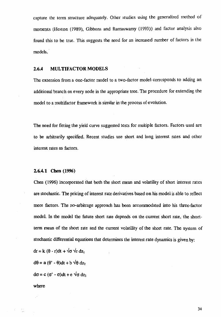
2.6.4.1 Chen (1996)

Chen (1996) incorporated that both the short mean and volatility of short interest rates

are stochastic. The pricing of interest rate derivatives based on his model is able to reflect

more factors. The no-arbitrage approach has been accommodated into his three-factor

model. In the model the future short rate depends on the current short rate, the short­

term mean of the short rate and the current volatility of the short rate. The system of

stochastic differential equations that determines the interest rate dynamics is given by:

dr = k (9 - r)dt + ~cr ..Jr dz1

de= a (9' - 9)dt + b ..Je dz2

dcr = c (cr'- cr)dt + e ..Jcr dz3

where

34

dr is the change in the future short rate r,

d8 is the change in the short-term mean of the short rate,

dais the change in the volatility of the short rate,

k, a and c are constants and arc the reversion rates of the short rate, shorHcrm mean of

the short rate and the volatility of the short rate.

Despite authors like Brennan and Schwartz (1979), Schaefer and Schwartz (1984),

incorporating more factors in their models; multifactor models are disadvantaged in that

they may not fit perfectly a given term structure.

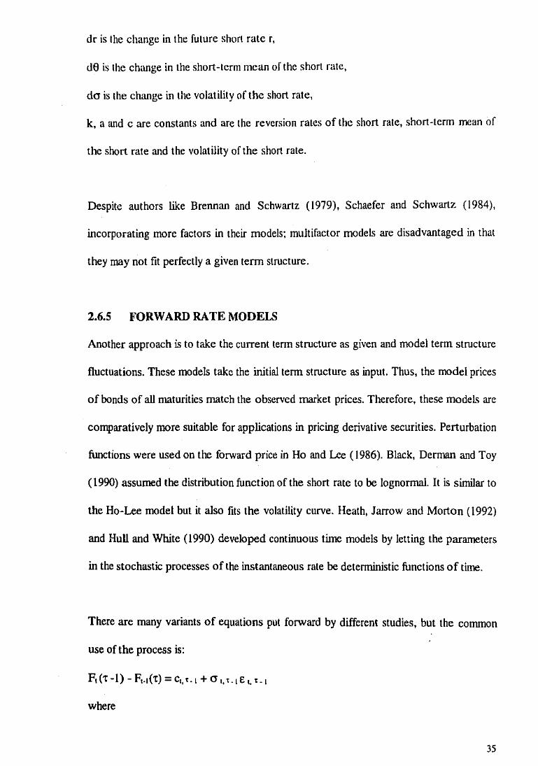
2.6.5 FORWARD RATE MODELS

Another approach is to take the current tenn structure as given and model term structure

fluctuations. These models take the initial term structure as input. Thus, the model prices

of bonds of all maturities match the observed market prices. Therefore, these models are

comparatively more suitable for applications in pricing derivative securities. Perturbation

functions were used on the forward price in Ho and Lee ( 1986). Black, Derman and Toy

(1990) assumed the distribution function of the short rate to be lognormal. It is similar to

the Ho-Lee model but it also fits the volatility curve. Heath, Jarrow and Morton (1992)

and Hull and White (1990) developed continuous time models by letting the parameters

in the stochastic processes of the instantaneous rate be detcnninistic functions of time.

There are many variants of equations put forward by different studies, but the common

use ofthe process is:

F,(t -1)- F,.1(t) = c,,t.l +a 1,t.1E '· 1:.1

where

35

F, (t -I) and F,. 1(t) arc the forward rates at different points m time and the other

parameters are constants.

The different models make different assumptions made about volatilities a 1. 1 . 1. The

model could have a constant volatility or a proportional volatility assumption. c1, t. 1 IS

the current price of the asset as given and it reflects the no-arbitrage assumption.

The equation used by HJM model for the evolution of the forward rate incorporates

spreads and changes in yields.

F,(t -I)- F,.1(t) = [1/t(t -l)]sp,(t)- [(t + !)/ t] (r, (t + I)- r, (t)) + [(t + l)i t] 11 r,(t +

I)- 1/t 11 r,(l)

For small 't, constant volatility models with martingale difference errors could not

describe the data. The rank of the covariance matrix of the errors E '· 1. 1 are generally

found to be two or three so the assumption of a single error to drive all forward spreads

proves to be unreliable.

2.6.5.1 Ho and Lee Model (1986)

Ho and Lee ( 1986) fmd that although the multi-factor models can improve the fitting of

the yield curve, they still do not perform well enough. Ho and Lee adopt the approach of

taking bond prices as given instead of pricing bonds. Therefore, their model cannot be

used to fmd bond prices. The model is mainly used for pricing interest rate contingent

claims.

36

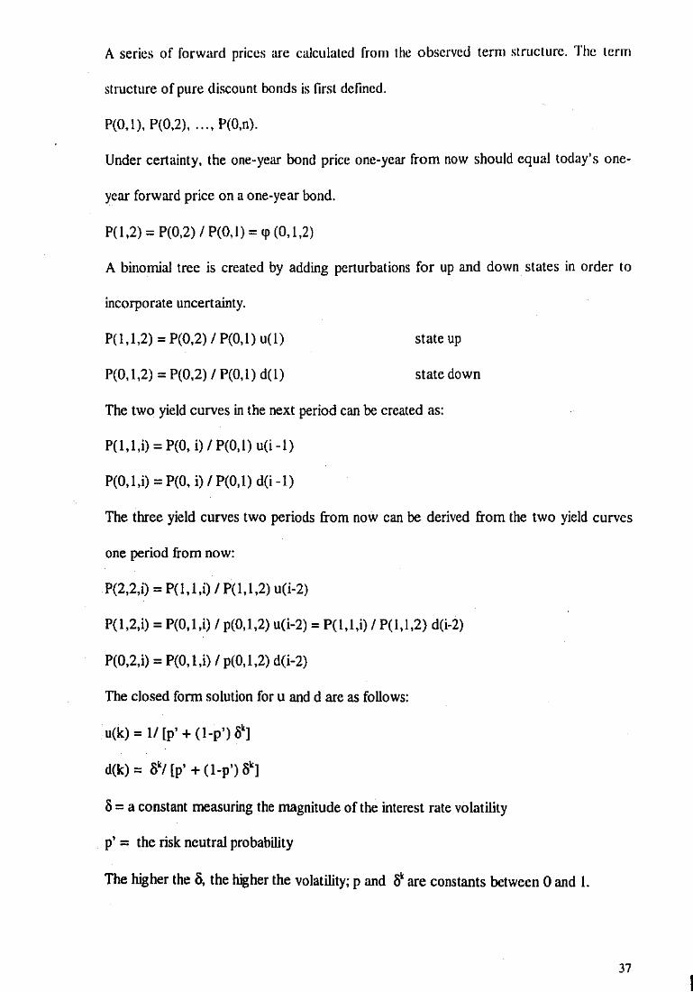
A series of forward prices are calculated from the observed term structure. The term

structure of pure discount bonds is first defined.

P{O,l), P{0,2), ... , P{O,n).

Under certainty, the one-year bond price one-year from now should equal today's one­

year forward price on a one-year bond.

P(l ,2) ; P(0,2) I P{O, 1) ; <p {0, 1 ,2)

A binomial tree is created by adding perturbations for up and down states in order to

incorporate uncertainty.

P{l,l,2); P(0,2) I P(O,l) u(l)

P(O,l,2); P(0,2) I P(O,l) d(l)

state up

state down

The two yield curves in the next period can be created as:

P{l,l,i); P{O, i) I P{O,l) u(i -1)

P(O,l,i); P{O, i) I P(O,l) d(i -1)

The three yield curves two periods from now can be derived from the two yield curves

one period from now:

P(2,2,i); P(l,l,i) I P(l,l,2) u(i-2)

P(l,2,i); P(O,l,i) I p{O,l,2) u{i-2); P(l,l,i) I P{l,l,2) d(i-2)

P(0,2,i); P(O, l,i) I p{O,l,2) d(i-2)

The closed form solution for u and d are as follows:

u(k); II [p' + (1-p') ~'1

d(k) ; '6'1 [p' + (1-p') ~·]

3 = a constant measuring the magnitude of the interest rate volatility

p' = the risk neutral probability

Tbe higher the '6, the higher the volatility; p and ~·are constants between 0 and 1.

37

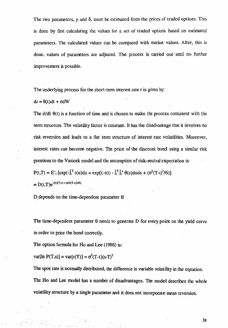
The two parameters, p and 6, must be estimated from the prices of traded options. This

is done by first calculating the values for a set of traded options based on estimated

parameters. The calculated values can be compared with market values. After, this is

done, values of parameters are adjusted. The process is carried out until no further

improvement is possible.

The underlying process for the short-term interest rater is given by:

dr = 8(t)dt + crdW

The drift 9(t) is a function of time and is chosen to make the process consistent with the

tenn structure. The volatility factor is constant. It has the disadvantage that it involves no

risk reversion and leads to a flat term structure of interest rate volatilities. Moreover,

interest rates can become negative. The price of the discount bond using a similar risk

premium to the Vasicek model and the assumption of risk-neutral expectation is:

P(t,T) = E', [exp(-J,T r(u)du = exp[(-r(t)- ),T),' 8(u)duds + (a'(T-t)3/6)]

= D(t,T)e·!{tXT·tl+Ca2cT-tJJf6J

D depends on the time-dependent parameter 8

The time-dependent parameter 8 needs to generate D for every point on the yield curve

in order to price the bond correctly.

The option formula for Ho and Lee (1986) is:

var[ln P(T,s)] = var[r(T)] = a'(T-t)(s-T)2

The spot rate is normally distributed, the difference is variable volatility in the equation.

The Ho and Lee model has a number of disadvantages. The model describes the whole

volatility structure by a single parameter and it does not incorporate mean reversion.

38

One problem with the Ho and Lee model is that it allows negative interest rates. This

issue was pinpointed by Ritchken and Boenawan (1990). The major difference between

the Ho and Lee model and other models is that Ho and Lee model the bond price process

while the others model the interest rate processes.

2.6.5.2 Hull and White Model (1990)

The model by Hull and White ( 1990) overcomes the defects of Ho and Lee. They discuss

how the one-factor models of Vasicek (1977) and CIR (1985) can be extended so that

they are consistent with both the current term structure of interest rates and the current

volatility of all spot rates or the current volatility of all forward rates. The underlying

distribution process is normal.

It is based on the equation:

dr = a(t)[u(t)- r]dt + a(t)dW

a(t) is a constant but also time dependent. The time varying parameters allow a better fit

of the model.

Hull and White (l990b) employ a trinomial method that allows for a different branching

procedure. The method permits the user to solve for different probabilities at each node,

which uphold tbe constraint that tbe probabilities must sum up to one and that they must

guarantee that the interest rate will be normally distributed with mean and variance

correctly defmed.

Hull and White (l990a) have proposed a modification to the model to incorporate the

current term structure. The extended Vasicek model is normally distributed and

39

parameters are time dependent. The market price of risk can be time dependent if the

parameters are time dependent. Hull and White obtain their solution by solving a partial

differential equation. The risk neutral process is as follows:

dr = [et(t)u(t)- crq(t)- a(t)r]dt + crdW

where q(t) is the market price of risk

The stochastic linear equation has the solution of:

r(s) = cp(s}[r(t) +I.' cp(u)" 1 [a(u)~(u)- crq(u)]du +I.' cp(u)"1crdW,

where Jjl(s) = exp(-1,' a(u)du)

The mean and variance of the state variables are:

E1[r(s)] = Jjl(s)[r(t) + I.' .p·'(u)q(u}du)]

cov, [r(s),r(u)] = Jjl(s)[ I,"''''·'1W1(w) cr)' dw] Jjl(u)

The term structure model will be:

P(t,T) = E, [exp(-l,r r(s)ds)] = em(<.T)>(V(<,TI/21

where

m(t,T) = l,r E'[r(s)]ds = l,r {Jjl(s}[(r(t) +I.' cp(u)"1 [a(u)~(u)- crq(u)]du]ds

V(t, T) = l,r 1,' 21<. [r(s),r(u)]duds = l,r I.' 2 cp(s) [I,"W1(w)cr)2 dw] Jjl(u)duds

a(t) and ~(t) have Jo be in closed form for the bond price

The pricing formula can generate any bond prices to match the observed ones traded in

the marketplace. The option formula of the model is based on a log normal distribution.

The option pricing formula is:

40

C(t, T" T) = P(t,T)N(d)- P(t, T,)KN(d- ,Jv,)

where

d = {ln(p(t, T)/KP(t,T,) + V,/2}/ ,)y,

V, = var(ln P(T,, T)) = F(T,, T)1 var(r(T,)) = F(T,, T)2 $( T,)2 <l )(' $(w)"'dw

When cr is known, the flexibility of !'(t) and rt(t) can be used to fit the yield curve. The

equation becomes a one~ time dependent parameter model if the model is not required to

fit the yield curve.

The bond and option formula become:

P(t,T) = E, [exp (-J,T r(s) ds)] = em(t.Tl+(V(t.TI]n

where

m(t,T) = r(t)F(t,T) + ).T [e"' .. ' d.' e"''·tl [rt!'(U)- crq(u)]du)]ds = r(t)F(t,T) + D(t,T)

V(t,T) =diet' [T-t-(e'atT·•J /2a.) + [2(e~rr·•J /a.)]- (3/2a.)

In order to fit all bond prices, D is used to provide flexibility. The yield curve can be

fitted without changing the option prices (but changing D) since the time dependent

parameters (!' and q) are not part of the equation.

Hull and White (1993) propose another variation of the model with a. being constant.

Tbeir model fits the current term structure to the model and updates the parameters as

they step through time. A disadvantage in this model is it recalibrates with no real time­

dependent structure. However, except for the Extended-Vasicek model, Hull and

White's (1990) approach provides no closed form solution and has to rely on numerical

methods.

4(

I

2.6.5.3 Heath-Jarrow·Morton (HJM) (1992)

Heath, Jarrow and Morton (1992) drop the path-independence condition of the Ho-Lcc

model. Forward rates are used as the primitive variables and they model the evolution of

an infmite set of forward rates.

The Ho·Lce, Vasicek and the Hull-White extension of the Vasicek model modelled the

short or the forward rates as Gaussian processes. Any model within the Heath-Jarrow­

Morton framework possessing a deterministic volatility will also give rise to a Gaussian

forward rate curve. The main defect of the model is that negative interest rates may be

generated with positive probability. If the existence of cash is an assumption, negative

interest rates would lead to theoretical arbitrage opportunities.

The HJM model is a framework under which all arbitrage-free term structure models can

be derived. Instead of using multi-factors as the state variables, their model takes the

entire forward rate curve as their state variable.

Attari (1997) describes how the HJM model is generated. First, the initial forward rate

curve and the volatility functions are used to specify the arbitrage-free movements in the

forward rates. This allows the computation of unique martingale probabilities which can

be used to price contingent claims. The price of a bond is:

P(t, T) = exp ( · l:j(t,j a)a)

where the forward rate f (t, T) at t for T to T + a is assumed to satisfy the stochastic

process

j(t, T) =j(O, n + l:aj[u1 (j6, T) · v1 (jA, T)] + 2: v1 (ja, T)]

42

The a; takes on values 0 or I with an objective probability given by q,(j). The u's and v's

are random functions that at each time t can depend on any information prior to time t.

The forward rate process is an arbitrage-free process.

Under a continuous time framework, only the forward rate volatility needs to be

specified. The forward rate at timet from timeT to timeT+ dT can be given byf(t, T).

The prices of discount bonds can then be specified in terms of the forward rates:

P(t, T) exp {- ),T f (t, v)dv )

The forward ratef(t, T) at timet can be given in terms of the initial forward ratef(O, T)

as:

f(t, T) =J(O, T) +lo'a(v, T, w)dv+ Ilo' cr; (v, T, w) dW; (v)

This is under the objective probabilities. The spot rate at timet isf(t, t) and is given as

r(t) = f(O, T) + Jo' a (v, T, w)dv +I Jo' cr; (v, T, w) dW; (v)

Using the forward rate and the spot rate the relative price of the bond is

Z (t, T) = P (t,T) I B(t) where B(t) = exp (io' r(y) dy)

The forward rate process under the risk-neutral measure is given as:

f (t, T) = f (0, T) +I. lo' cr; (v, T) ),' cr; (v, y) dy dv + L Jo' cr; (v, T) dW; (v)

By specifying! (0, T) and cr; ,J (t, T) can be obtained.

The forward rate can be expressed as:

df(t, T) = a.(t,T)dt + cr(t,T)dW

Bond price and the forward rate volatility need to be a function of time to maturity.

Discount bonds can be priced when f (t, T) is found and contingent claims C(t) can be

priced using:

43

C(t) = B(t) E,* (C(T) I B(T))

where E1* is the expectation computed using the risk-neutral probabilities

One drawback of the Heath-Jarrow-Morton model is that the interest rate models

resulting from their approach are usually non-Markov. Because the HJM model is a

generalization of the Ho and Lee model that is obtained by dropping the path­

independence condition, the forward rates are path dependent and the resulting tree does

not recombine. The distribution of interest rates in the next period depends not only on

the current rate but also on the rates in the earlier periods. Moreover, there are only a

small number of known forward rate volatility functions that give rise to the Markov

models (Chen (1996a)). It is difficult to derive closed-fom1 solutions for the values of

bond and interest rate derivatives. However, if the path dependence can be represented

by a single statistic, the evolution of the term structure can then be characterized by just

the spot rate. This reduces the computational complexity of the model.

Abken (1993) fitted HJM models to forward rates by the generalized method of

moments whilst Amin and Morton (1994) used option prices to recover implied

volatilities whose evolution was compared to those of the most popular variants of the

HJM model. Abken demonstrates that the latter tends to follow a constant volatility

formulation and the former tends to follow a proportional one. It is important to examine

the evidence regarding volatility together with model specifications.

Amin and Morton (1994) tested six models in the HJM class. The models tested have the

implied volatility function of:

a(.)= [ao+ a,T- t] exp[-A(T-t)]f(t, T)'

44

Data on Eurodollar futures and options contracts arc tested. Two parameter models tit

observed option prices better than single parameter models but the results arc

inconsistent. Their results support those of Flesakar ( 1993) who uses data on Eurodollar

futures options.

All the time-dependent parameter models are similar in that the parameters are adjusted

to fit the observed yield and volatility curves. When a normal distribution is assumed, all

models can be translated to one another. When pricing American contracts, the Hull and

White model is the most suitable for the lattice framework. It provides the simplest way

to build the model when numerical methods are required to price the options. Only the

short rate is used in pricing compared to the HJM model which requires a set of points

on the forward rate or the short rate curves. The various approaches and model

specifications are summarised in Table 2 below.

I.Thk 2 lli'H'Iopnwnh in ll'TIII "itrudl1!'l' \loddill'..! II . .J,l·n h·om ( lu·uii 1JI}(I,tll

Authors Merton (1973) Vasicek ( 1977) Brennan-Schwartz ( 1979)

Dothan ( 1978) Schaefer-Schwartz ( 1984)

Cox-Ingersoll-Ross ( 1985) Ho-Lee (1986) Black-Derman-Toy ( 1990) Hull-White (1990) Heath-Jarrow-Morton (1992) Longstaff-Schwartz (1992)

Chen (1994)

Model Specifications

dr = 9dt + adz dr = k(9- r)dt + crdz dr = 9rdt + O'rt dz1 + O'r2 dz2 dl = ~dl + O"u dz, + CJ,z dzz dr = crrdz ds = m(J.l- s)dt + 11 dz 1

dl = m(a'-ls)dt +eN! dz2

dr = k(9- r)dt + cr-lrdz dr = edt + crdz dIn r = (9- o'(t)lcr(t)ln r]dt + o(t)dz dr = k(9- r)dt + crJrdz df = a(t)dt + cr(t)dW dy1 =(a- b y1)dt + d y1dW1

dy2 = (k- e y2)dt + f~ y1dW2 dr = k (9- r)dt + ,Ja Vr dz1

d9 =a (9' - 9)dt + b .Je dz2

dcr = c (a' • cr)dt + e Vcr dz3

8, cr are constants k, 8, cr are constants ar • e, . cr., . 0',2 ' O"a • 01~ are constant cr is constant m, J.l, 11. 0' are constant

k, 9, a are constants e time varying, cr constant e is time varying e. a are time varying f is the forward rate a, b, k, e are constant

k, a, 9'. b, c, cr', care constant

45

Eurodollar futures and futures options arc tested usmg the HJM approach using the

Generalized Method of Moments with three years of daily data (Flesaker (1993)). He

concludes that the approach is not compatible with the data for most periods. Backus,

Foresi and Zin (1994) demonstrate that the Black, Derman and Toy model is likely to

overprice call options on long bonds when interest rates exhibit mean reversion. They

find that the no-arbitrage term structure model can lead to systematic arbitrage

opportunities as a result of its mispricing of some assets. Mispricing can also occur when

no other traders offer the mispriced assets. They conclude that the empirical results are

disappointing.

The problem with the no-arbitrage models of Ho and Lee ( 1986), Heath-Jarrow-Morton

(1992), Hull and White (1990, 1993), Black, Derman and Toy (1990) is that on any day

a function for the term structure of interest rates needs to be estimated and there is no

guarantee that the estimated function will be consistent with the previously estimated

one. Although this approach has the ability to fit the initial term structure, its empirical

perfonnance is not sound.

2.7 . NEW DIRECTIONS

PoiJ.it Process Models

Researchers introduced jumps due to the empirical evidence that interest rate path

movements cannot be represented by diffusion processes. Instead, they behave more like

pure jump processes. This is why point process models are introduced and this theory

has been actively discussed currently in the literatt~re.

46

Daz (1995) uses a jump-diffusion process for the short-term interest rate. A jump­

diffusion process is suitable as the changes in short-term interest rate have too many

outlying values to be generated by one diffusion process alone. Daz obtains expressions

for discount bond prices in the presence of jumps. Option prices can also be computed in

an equilibrium model where the short-term interest rate follows a jump-diffusion process

(Attari 1996).

Shirakawa (1991), Bjork (1995) and Jarrow-Madan (1995) consider interest rate models

driven by a finite number of counting processes. Jarrow and Madan construct a 1J10del

for asset prices driven by semimartingales. Bjork, Kabanov and Runggaldier (1995)

modeled the forward rates as:

df(t, T) = a(t, T)dt + O'(t, T)dW, + JE 0 (t, x, T)~(dt, dx)

where:

Jl is a multivariate point process.

It covers the case of a flnite number of driving counting processes as well as the case of

an infmite mark space E. The inclusion of the infmite mark space into the model will

introduce an infmite number of random sources. The measure-valued portfolios which at

each point in time contain bonds with a continuum of maturities have to be used in order

to produce any effect of hedging. Suppose the number of bonds held at time t is denoted

by h(t, dT) with maturities in the interval [T, T + dT] and g(t) is tbe number of units of

the risk free asset B. The definition of the value process becomes:

V(t) = g(t) B(t) + ),- p(t, T) h(t, dT)

The formal generalization of the standard self-financing condition can be summarized as:

dV(t) = g(t)dB(t) + ).- h(t, dT)dp(t,T)

47

Bjork, Kabanov and Runggaldier (I 995) find that the standard portfolio concept can be

extended to include measure valued portfolios. The no-arbitrage condition on the interest

rate dynamics can provide an extension of the HJM condition. They conclude that as

opposed to the standard models with only a finite set of assets, market completeness is

no longer equivalent to uniqueness of the martingale measure. It is shown that the

uniqueness of the martingale measure is equivalent to 'approximate completeness' of the

market. In this case, claims belonging to a dense subspace of the space of all claim<; can

only be hedged.

2.8 IMPLICATIONS

In summary, the literature has been concentrated in empirical research on single and

multifactor models. The analysis in the use of time·dependent models is very limited.

This is true especially in the Australia context. There are many questions required to be

j'Jstified including how pricing errors are affected by time to maturity, the degree in

which options are in and out-of-the-money and volatility? What are the deviations of

pricing errors when different models are used? How do they differ? This study addresses

these issues by using call options on 90·day Bank Accepted Bill futures as taken from the

Sydney Futures Exchange in order to investigate the accuracy of different pricing

methods.

48

Chapter 3: METHODOLOGY

3.1 DESiGN

Monthly data is used taken from the year 1996 to price call options on 90 Day Bank

Accepted Bill Futures from the period I January 1996 to 31 December 1996. The futures

and options data are closing prices taken from the la'it Wednesday of the month to

ensure consistency. Despite the fact that options are priced on individual days, interest

rates and reversion rates are generated on a continuous basis using the yield curve,

volatilities and reversion rates generated each month at that point in time from interest

rate caps and market data at that point in time. (This is hctter explained in Part 3.3

Parameter Estimation).

Both the option and the futures data were collected from the Sydney Futures Exchange

(SFE) web site directly from the internet. Each futures trade and option is matched

according to the futures prices at the end of a particular day since prices are quoted on

the end-of-the-day basis. (Thus, there may he a problem with lack of data synchronicity

as the end of day prices may not represent trades made at identical times).

The bank bill market is the largest short-term interest rate market in Australia. Bank

Accepted Bills are negotiable short-term securities used to affect short-tenn borrowing

and lending for periods typically between 30-180 days. A Bank Bill represents a promise

to pay the full face value of the bill at maturity with its credit risk based on the debt

rating of the bank which guaranteed its payment. Bank bills are quoted on a yield per

cent per annum basis and are priced according to a yield fonnula that discounts the face

value to earn the appropriate interest cost.

49

Options on Bank Bill futures are American style options. Future options are marked to

market on a daily basis, profits and losses are withdrawn and paid as they accrue. When

the position is marked to market at the end of the day, the holder of a call option can

withdraw any excess of the futures price over the exercise price. The holder of the put

option can withdraw any excess of exercise price over futures price. The futures contract

is left with no value when it is closed out. The use of appropriate models (i.e., reflecting

margining) are needed to price these options. Both the Extended-Vasicek and HJM

Model, as applied in this work, incorporate adjustments for marking-to-market futures

style. The Asay Model, as discussed before, is derived principally to price futures or

options that are subject to futures style margining. Despite the fact that the Black model

is similar to the Asay Model and the Asay model is derived from the former, the Black

model calculates the present value of the exercise price which is inappropriate for futures

style margining. In this study, however, the Black model is aJso used for comparison to

the other models to investigate how prices change when the marking-to-market property

is not including in pricing.

The face value of the 90-Day Bank Accepted Bill futures contract is A$500,000. The

delivery months are the spot month (nearest) and the next consecutive months. March,

June, September and December quarters are then traded up to two years ahead. Eight

quarter months are available for trading with strike prices at 0.25% intervals. As the 90-

Day Bank Bill contract involves physical delivery, options expire five days prior to

futures expiry so as to close or adjust positions. The market convention is to quote th~'

option premium as yield per cent per annum x 100 (basis points). The dollar value of an

option premium is calculated by comparing its contract value at the strike price and the

value at the same price minus 0.0 I%. Quotes are expressed as an index (I) equals to

50

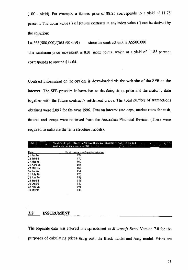
(100- yield). For example, a futures price of 88.25 corresponds to a yield of 11.75

percent. The dollar value (f) of futures contracts at any index value (I) can be derived by

the equation:

f; 365(500,000)/(365+90-0. 91) since the contract unit is A$500,000

The minimum price movement is 0.0 I index points, which at a yield of I I .85 percent

corresponds to around $11.64.

Contract information on the options is down-loaded via the web site of the SFE on the

internet. The SFE provides information on the date, strike price and the maturity date

together with the future contract's settlement prices. The total number of transactions

obtained were 2,097 for the year 1996. Data on interest rate caps, market rates for cash,

futures and swaps were retrieved from the Australian Financial Review. (These were

required to calibrate the tenn structure models).

l.thhl ' \nmln'rol!,lllllp11"!l'"n'Hl·ll,nll.nth\<<<phtl,lhll-lr,ul\ll.r11hll,r•t , o • ,

Date 31Jan96 28 Feb96 27 Mar96 24 April96 29 May96 26Jun 96 31 July96 28 Aug96 25 Sep96 30 Oct 96 27 Nov96 18 Dec96

3.2

\\tllru•ll.ll o( lho lll<nrlh 111 1'111r, ' •'

No oroontrags wjth settlemelll udro

INSTRUMENT

174 170 169 168 165 !57 170 182 183 180 191 188

The requisite data was entered in a spreadsheet in Microsoft Excel Version 7.0 for the

purposes of calculating prices using both the Black model and Asay model. Prices are

51

calculated based on the relevant formulas entered. Prices for the other models were

calculated using the Optimum: Fixed lflcome Monis Software which takes data required

to calibrate the yield curve and calculates the theoretical price of an interest rate option

using the calibrations.

The pricing of the options on futures is based on the Heath, !arrow, Morton ( 1992) and

the Extended-Vasicek ( 1989) models. The actual valuation formulae and tree

implementation are built in the software and are shown below:

o The Extended-Vasicek Model

dP(t,T) = ~.(t, T)P(t, T)dt + cr,(t, T)P(t, T)dZ.

where:

T is the bond maturity time

2,. is a standard Brownian motion

O'a is a deterministic function given by:

for positive constants a and O'a

cr,(t, T) = ( cr,/ll)(l-exp( -a(T-t)))

The associated short rate satisfies the stochastic differential equation

dr(t) = a(m(t) - r(t))dt + cr,ctz,

The function m(t) is the mean level of the short rate. The parameter a is the reversion

rate, and O"a is the Vasicek volatility.

• · The HJM model

Uses two factors with deterministic volatility functions

The bond price is given by:

dP(t, T) = ~,(t, T)P{t, T)dt + O'bi(t, T)P(t, T)dW, + cr,2(t, T)P(t, T)dZ.

where Wand Z are independent standard Brownian motions

52

crb2(t, T) is as in the Extended-Vasicek model

crb1(t, T) is given by crb1(t, T) = crb1(T - t)

The short rate is not a Markov process, so has a less convenient stochastic differential

equation. The forward rate has the form of:

df(t, T) = v(t, T)dt + crb1dW1 + crb2 exp(-a(T-t))dZt

The software permits the taking into account of the futures style margining feature of

trading on the SFE in order to make the analysis consistent when the results from the

above models are compared to the Asay model's.

The advanced statistical software package SPSS for Windows, Release 7.0 was used to

assist the analysis of data. The Shazam econometrics software package was used to run

the Ordinary Least Square Regressions.

3.3 PARAMETER ESTIMATION

3.3.1 BLACK MODEL

3.3.1.1 Time to Maturity

Call options become more valuable as the time to expiration increases. Options on 90

day Bank Accepted Bill futures mature every three months. The time to maturity is

obtained by dividing the number of days-to-maturity by the number of days in a year

(365).

53

3.3.1.2 Volatility

Volatility measures the uncertainty of future stock price movements. The holder of a call

benefits from a price increase; whereas the owner of a put benefits from a price decrease.

The value of call prices increase as volatility increases. Implied volatility is used to

monitor the market's opinion about the volatility of a particular option.

Latane and Rendleman (1976), Chiras and Manaster (1978) and Brown and Shevlin

(1983) found that implied volatility is a more efficient predictor of options prices than

historical volatility measures. Implied volatilities are taken from SFE accompanied by

each of the option contracts. The fact that implied volatilities were taken from the

exchange, should if anything, favour the Black and Asay models in the empirical tests. It

may also lead to subtle biases in that the Vega of a European call option on a non­

dividend-paying stock is given by:

Vega= S(T-t) 112 N'(d1 )

where

S represents the value of the underlying security,

T-t is the time to maturity of the option,

N is the cumulative normal distribution

d1 is as defined below.

The above suggest that estimates of the implied volatility will be sensitive to the level of

the stock price and the time to maturity. This may affect the degree of pricing errors

across different option series and maturities when the Black and Asay models are

applied.

54

The Black (1976) model used to price the 90-day Bank bill options can be described by

the following formula:

where

d1 = [ ln(F/X) + <rT/2]/ (CJ"liT) d2 = [ ln(F IX) - cr2T /2 ]/ ( CJ"liT) = d I - CJ"liT

N(.) is the cumulative probability function for a standardized normal variable,

c and pare European call and put prices,

F is the futures price,

X is the strike price, r is the risk-free interest rate,

T is the time to expiration, and cr is the volatility of the bond price.

The following assumptions are made when using the model proposed by Black.

1) The futures price Fis a continuous-time stochastic process that can be represented by

the stochastic differential equation:

dF/F = µdt + adz

where dz is a Wiener process.

2) There are no transaction costs.

By invoking the condition that no risk-free arbitrage opportunities exist in an efficient

market.

3.3.2 ASAY MODEL

The SFE trade options on futures where the options have futures-style margining. Option

contracts are marked to market at the end of the day like futures contract. Thus, another

55

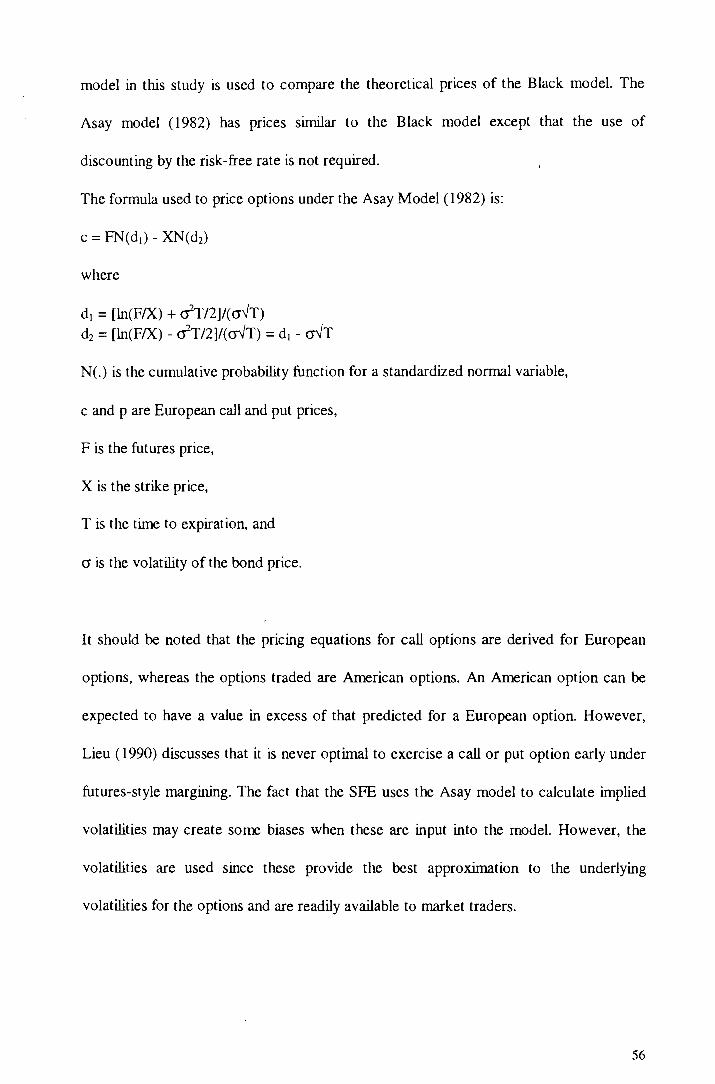
model in this study is used to compare the theoretical prices of the Black model. The

Asay model (1982) has prices similar to the Black model except that the use of

discounting by the risk-free rate is not required.

The formula used to price options under the Asay Model ( 1982) is:

where

d1 = [ln(F/X) + crT/2]/(mfT) d2 = [ln(F/X) - crT/2]/(mfT) = d1 - mfT

N(.) is the cumulative probability function for a standardized normal variable,

c and p are European call and put prices,

F is the futures price,

Xis the strike price,

T is the time to expiration, and

cr is the volatility of the bond price.

It should be noted that the pricing equations for call options are derived for European

options, whereas the options traded are American options. An American option can be

expected to have a value in excess of that predicted for a European option. However,

Lieu ( 1990) discusses that it is never optimal to exercise a call or put option early under

futures-style margining. The fact that the SFE uses the Asay model to calculate implied

volatilities may create some biases when these are input into the model. However, the

volatilities are used since these provide the best approximation to the underlying

volatilities for the options and are readily available to market traders.

56

3.3.3 THE TERM STRUCTURE MODELS

3.3.3.1 The Yield Curve, the Extended V asicek volatility, the HJM volatility and

the Reversion Rates

The yield curve is generated from market data. This is done by a standard bootstrapping

method. Market Rates for the last Wednesday of the month are gathered. Cash market

infonnation used includes both the offer and bid prices for overnight, one week, .one

month, two months, three months, six months and up to nine months maturity interest

rates. Prices of futures with maturity from three months up to three years are included.

Swap market prices with expiry from one year's time up to 10 year's time are also

entered for bootstrapping. The cash, futures, and swap market prices collected at the last

Wednesday of the months from January to December 1996 are shown in Tables 4-9.

The cash market is used as far as the futures market, which takes priority over

everything. The swap market is used for the longer dated points, with intermediate swap

rates found by interpolation if they are missing. There is an adjustment on the futures

market data to allow for the volatility of interest rates for the more advanced models.

The true futures' price was used rather than forward prices. Interest rate caps with

maturity one, three and fives years for each month are also added.

The method of Cubic Splines is used as the interpolation method. Data is converted into

discount factors at each known time point, and these are connected with cubic splines,

which preserve continuity of the first derivative of the discount factors at each time

point.

57

3.4 DA TA PROCESSING PROCEDURE

3.4.1 Black Model and Asay Model

After the parameters for volatility and risk-free rates have been estimated, they are

plugged into a spreadsheet containing the pricing formula for call options for Black

Model. The time to maturity is on a 365 day basis for a year.

3.4.2 The Tenn Structure Models

The current term structure is formulated by entering the current market values of market

rates for cash, futures, and swaps in the 'Market Rates' worksheet. The software

calculates the yield curve from the input data by the bootstrapping method. The start

date and number of points are automatically displayed. The yield curves generated for

each of the months in 1996 are shown in Tables 10-11.

The volatilities and the reversion rates are generated by entering the data for three

interest rate caps as quoted in the market on the same day. Interest rate caps are

derivative securities which restrict the rate of interest that can apply to floating-rate

loans. It is a contract where the seller of the contract promises to pay a certain amount of

cash to the holder of the contract if the interest rate exceeds a certain predetermined

level (the 'cap rate') at some future date. If a loan is taken at a floating rate of interest,

the investor may buy a cap from the bank in order to ensure that he/she will never have

to pay more than the cap rate. In the same way, the seller of a floor contract promises to

pay cash if some future interest rate falls below a certain predetermined level.

58

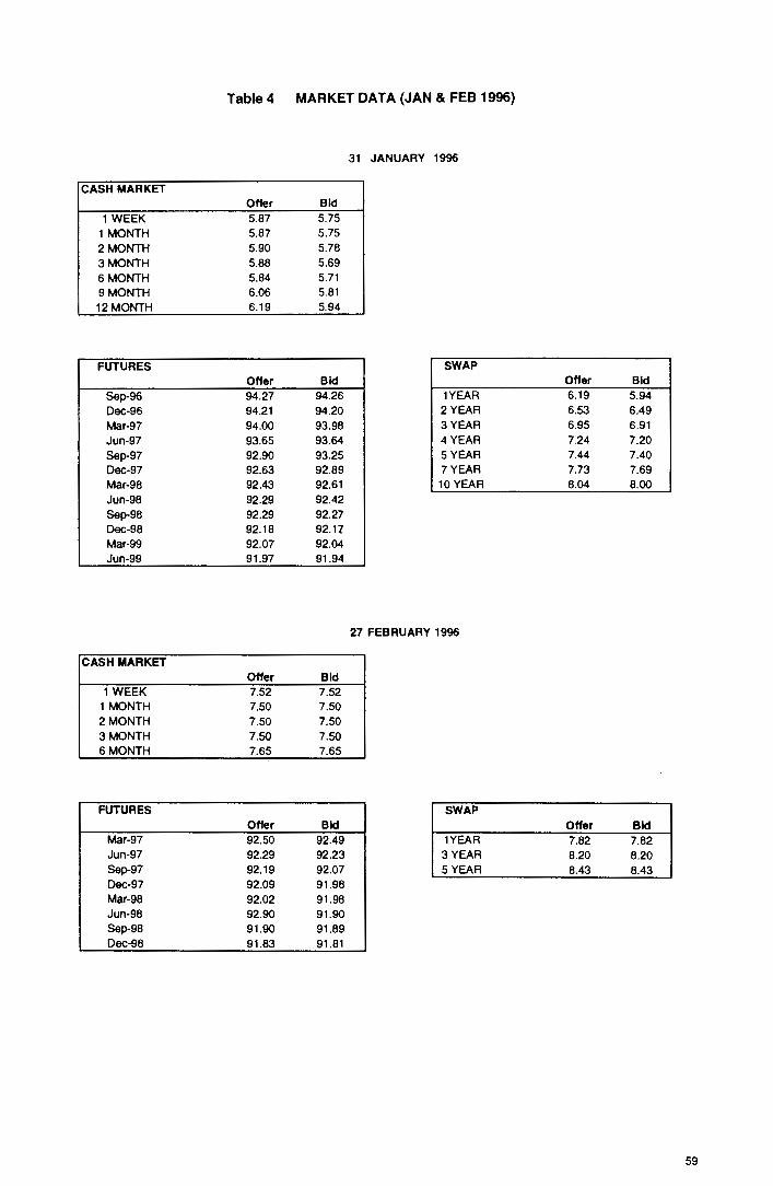
CASH MARKET

1 WEEK 1 MONTH 2MONTH 3MONTH 6 MONTH 9MONTH 12MONTH

FUTURES

Sep-96 Dec-96 Mar-97 Jun-97 Sep-97 Dec-97 Mar-98 Jun-98 Sep-98 Dec-98 Mar-99 Jun-99

CASH MARKET

1 WEEK 1 MONTH 2 MONTH 3MONTH 6MONTH

FUTURES

Mar-97 Jun-97 Sep-97 Dec-97 Mar-98 Jun-98 Sep-98 Dec-98

Table 4 MARKET DATA (JAN & FEB 1996)

Offer 5.87 5.87 5.90 5.88 5.84 6.06 6.19

Offer 94.27 94.21 94.00 93.65 92.90 92.63 92.43 92.29 92.29 92.18 92.07 91.97

Offer 7.52 7.50 7.50 7.50 7.65

Offer 92.50 92.29 92.19 92.09 92.02 92.90 91.90 91.83

Bid 5.75 5.75 5.78 5.69 5.71 5.81 5.94

Bid 94.26 94.20 93.98 93.64 93.25 92.89 92.61 92.42 92.27 92.17 92.04 91.94

Bid 7.52 7.50 7.50 7.50 7.65

Bid 92.49 92.23 92.07 91.98 91.98 91.90 91.89 91.81

31 JANUARY 1996

SWAP

1YEAR 2YEAR 3YEAR 4 YEAR 5 YEAR 7YEAR 10 YEAR

27 FEBRUARY 1996

SWAP

1YEAR 3YEAR 5YEAR

Offer Bid 6.19 5.94 6.53 6.49 6.95 6.91 7.24 7.20 7.44 7.40 7.73 7.69 8.04 8.00

Offer Bid 7.82 7.82 8.20 8.20 8.43 8.43

59

CASH MARKET

OVERNIGHT 1 MONTH 2MONTH 3MONTH 6MONTH

FUTURES

Jun-96 Sep-96 Dec-96 Mar-97 Jun-97 Sep-97 Oec-97 Mar-98 Jun-98

CASH MARKET

OVERNIGHT 1 MONTH 2MONTH 3MONTH 6MONTH

FUTURES

Jun-96 Sep-96 Dec-96 Mar-97 Jun-97 Sep-97 Dec-97 Mar-98 Jun-98 Sep-98 Dec-98

Table 5 MARKET DATA(MAR & APRIL 1996)

7.55 7.52 7.53 7.56 7.66

Offer 92.37 92.08 91.82 91.63 91.51 91.43 91.38 91.32 91.26

Offer 7.55 7.52 7.54 7.55 7.67

Ofler 92.42 92.24 91.93 91.65 91.48 91.29 91.24 91.10 91.18 91.04 91.01

Bid 7.55 7.52 7.53 7.56 7.66

Bid 92.35 92.04 91.77 91.59 91.46 91.38 91.34 91.28 91.26

Bid 7.55 7.52 7.54 7.55 7.67

Bid 92.37 92.09 91.72 91.42 91.27 91.17 91.11 91.07 91.06 91.03 91.00

27 MARCH 1996

SWAP

1YEAR 3 YEAR SYEAR

23 APRIL 1996

SWAP

1YEAR 3YEAR SYEAR

Off .. Bid 7.90 7.90 8.39 8.39 8.63 8.63

Offer Bid 7.85 7.85 8.37 8.37 8.57 8.57

60

CASH MARKET

OVERNIGHT 1 MOI\!TH 2MONTH 3 MONTH 6MONTH

FUTURES

Jun-96 Sep-96 oec-96 Mar-97 Jun-97 Sep-97 Dec-97 Mar-98 Jun-98 Sep-98 Dee-se Mar-99

CASH MARKET

OVERNIGHT 1 MONTH 2MONTH 3MONTH 6MONTH

FUTURES

Sep-96 Dec-96 Mar-97 Jun-97 Sep-97 Dec-97 Mar-98 Jun-98 Sep-98 Oec-98 Mar-99 Jun-99

Table 6 MARKET DATA (MAY & JUNE 1996)

Offer 7.50 7.52 7.53 7.55 7.63

Offer 92.47 92.43 92.09 91.80 91.56 91.41 91.28 91.23 91.18 91.14 91.10 91.06

Offer 7.35 7.52 7.55 7.60 7.70

Offer 92.34 92.10 91.81 91.58 91.43 91.31 91.25 91.21 91.17 91.13 91.08 91.03

Bid 7.50 7.52 7.53 7.55 7.63

Bid 92.46 92.32 92.05 91.75 91.54 91.39 91.27 91.22 91.17 91.12 91.08 91.03

Bid 7.35 7.52 7.55 7.60 7.70

Bid 92.32 92.06 91.77 91.53 91.38 91.29 91.25 91.19 91.16 91.12 91.08 91.03

29 MAY 1996

SWAP

1YEAR 3YEAR SYEAR

26 JUNE 1996

SWAP

1YEAR 3YEAR SYEAR

Offer Bid 6.19 5.94 6.95 6.91 7.44 7.40

Offer Bid 7.91 7.91 8.42 8.42 8.63 8.63

61

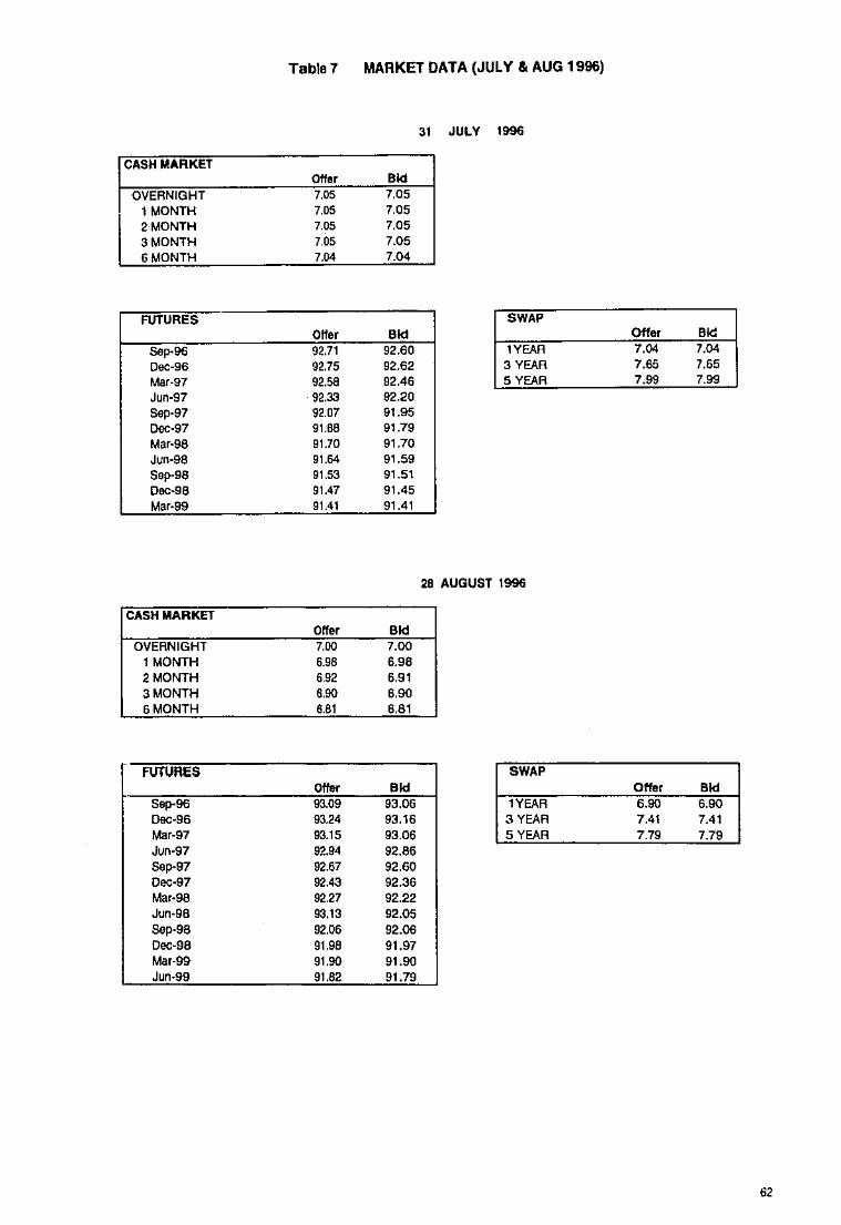
Table 7 MARKET DATA (JULY & AUG 1996)

31 JULY 1996

CASH MARKET Otter Bid

OVERNIGHT 7.05 7.05 1 MONTH 7.05 7.05 2MONTH 7.05 7.05 3 MONTH 7.05 7.05 6 MONTH 7.04 7.04

FUTURES SWAP Offer Bid Off•• Bid .. ,. .. 92.71 92.60 lYEAR 7.04 7.04

Dec-96 92.75 92.62 3 YEAR 7.65 7.65 Mar-97 92.58 92.46 5 YEAR 7.99 7.99

Jun-97 92.33 92.20 Sep-97 92.07 91.95 Dec-97 91.68 91.79 Mar-98 91.70 91.70 Jun-98 91.64 91.59 Sep-.98 91.53 91.51 Dec-sa 91.47 91.45 Mar-99 91.41 91.41

28 AUGUST 1996

CASH MARKET Orte• Bid

OVERNIGHT 7.00 7.00 1 MONTH 6.98 6.98 2MONTH 6.92 6.91 3MONTH 6.90 6.90 6MONTH 6.81 6.81

FUTURES SWAP

Offe• Bid Ofle• Bid Sep-96 93.09 93.06 tYEAR 6.90 6.90 Dec-96 93.24 93.16 3YEAA 7.41 7.41 Mar-97 93.15 93.06 SYEAR 7.79 7.79 Jun-97 92.94 92.86 Sap-97 92.67 92.60 oec-97 92.43 92.36 Mar-98 92.27 92.22 Jun-98 93.13 92.05 Sep-98 92.06 92.06 oec-98 91.98 91.97 Mar-99 91.90 91.90 Jun·99 91.82 91.79

62

TableS MARKET DATA (SEP & OCT 1996)

25 SEPTEMBER 1996

CASH MARKET Offer ·~ OVERNIGHT 7.00 7.00

1 MONTH 6.98 6.98 2 MONTH 6.91 6.91 3 MONTH 6.90 6.90 6MONTH 6.81 6.81

FUTURES SWAP Offer ·~ Offe< ·~ Sep-96 93.09 93.06 1YEAR 6.90 6.90

Oec-96 93.24 93.16 3YEAR 7.41 7.41 Mar-97 93.15 93.06 5YEAR 7.79 7.79 Jun-97 92.94 92.86 Sep-97 92.67 92.60 Dec-97 92.43 92.36 Mar-98 92.27 92.22 Jun-98 93.13 92.05 Sep-98 92.06 92.06 Dec-98 91.98 91.97 Mar-99 91.90 91.90 Jun-99 91.82 91.79

30 OCTOBER 1996

CASH MARKET Offer ·~ OVERNIGHT 7.05 7.05

1 MONTH 6.77 6.77 2MONTH 6.67 6.67 3 MONTH 6.59 6.59 6 MONTH 6.55 6.55

FUTURES SWAP Offe• ·~ Offe• Bid

O.C-96 93.54 93.50 1YEAR 6.47 6.47 Mar-97 93.67 93.64 3 YEAR 6.93 6.93 Jun-97 93.63 93.59 5YEAA 7.25 7.25 Sep-97 93.46 93.44 oec-97 93.28 93.24 Mar-98 93.07 93.05 Jun-98 92.94 92.92 Sep-98 92.84 92.83 Dec-98 92.75 92.75

63

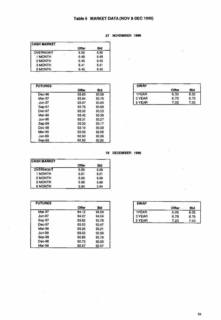
Table 9 MARKET DATA (NOV & OEC 1996)

27 NOVEMBER 1996

CASH MARKET Offer Bid

OVERNIGHT 6.50 6.50 1 MONTH 6.49 6.49 2MONTH 6.45 6.45 3 MONTH 6.41 6.41 6MONTH 6.40 6.40

FUTURES SWAP Offer Bid Offer Bid

Dec-96 93.60 93.58 WEAR 6.33 6.33 Mar-97 93.84 93.75 3YEAA 6.70 6.70 Jun-97 93.87 93.80 SYEAR 7.03 7.03 Sep-97 93.76 93.68 Dec-97 93.56 93.53 Mar-98 93.42 93.39 Jun-98 93.31 93.27 Sep-98 93.20 93.17 Dec-98 93.10 93.09 Mar-99 93.00 92.99 Jun-99 92.90 92.89 Seo-99 92.80 92.80

18 DECEMBER 1996

CASH MARKET Offer Bid

OVERNIGHT 6.00 6.00 1 MONTH 6.01 6.01 2 MONTH 6.00 6.00 3 MONTH 5.99 5.99 6 MONTH 5.94 5.94

FUTURES SWAP Offer Bid Offer Bid

Mar-97 94.12 94.09 1YEAR 6.06 6.06 Jun-97 94.07 94.04 3YEAA 6.78 6.76 Sep-97 93.82 93,78 SYEAA 7.23 7.23 Dec-97 93,53 93.47 Mar-98 93.26 93.21 Jun-98 93.03 92.99 Sep-98 92.85 92.79 Dec-98 92.73 92.69 Mar-99 92.57 92.57

64

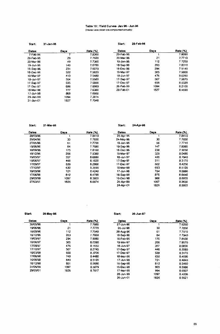
Start: 31-Jan-96

Dates Days 7-Feb-96 7

29-Feb-96 29 20-Mar-96 49 19-Jun-96 140 18-Sep-96 231 18-0ec-96 322 19-Mar-97 413 18-Jun-97 504 17-Sep-97 595 17-0ec-97 686 18-Mar-98 777 17-Jun-98 868 29-Jan-99 1094 31-Jan-01 1827

Start: 27-Mar-96

Dates Days 28/03/96 1 29/04/96 33 27/05/96 61 19/06/96 84 18/09/96 175 18/12196 266 19/03/97 357 18/06/97 448 17109/97 539 17/12197 630 18/03/98 721 17/06/98 812 29/03/99 1097 27/03/01 1826

Start: 29-May-96

Datea Days 30/05/96 1 19/06/96 21 18/09196 112 18/12196 203 19/03/97 294 18/06/97 385 17/09/97 476 17/12197 567 18/03/98 658 17/06/98 749 16/09/98 840 16/12198 931 31/05/99 1097 29/05/01 1826

Table 1 O : Yleld Curvea- Jan 96 - Jun 96 (Interest rates shown are compounded 8/VlUaJty)

Start: 28-Feb-96

Rate(%) Datea 7.8360 29-Feb-96 7.7620 20-Mar-96 7.7360 19-Jun-96 7.6780 18-Sep-96 7.6070 18-Dec-96 7.5620 19-Mar-97 7.5480 18-Jun-97 7.5580 17-Sep-97 7.5800 17-0ec-97 7.6080 26-Feb-99 7.6380 28-Feb-01 7.6660 7.3814 7.7048

Start: 24-Apr-96

Rate(%) Dates 7.8410 25-Apr-96 7.7830 24-May-96 7.7700 19-Jun-96 7.7680 18-Sep-96 7.8160 18-0ec-96 7.9380 19-Mar-97 8.0680 18-Jun-97 8.1830 17-Sep-97 8.2800 17-Dec-97 8.3590 18-Mar-98 8.4240 17-Jun-98 8.4790 16-Sep-98 8.3920 16-0ec-98 8.6674 26-Apr-99

24-Apr-01

Start: 26-Jun-97

Rate(%) Datea 7.7880 27-Jun-96 1.mo 26-Jul-96 7.7540 26-Aug-96 7.7930 18-Sep-96 7.9080 18-Feb-96 8.0390 19-Mar-97 8.1650 18-Jun-97 8.2740 17-Sep-97 8.3700 17-Dec-97 8.4480 18-Mar-98 8.5120 17-Jun-98 8.5680 16-Sep-98 8.5679 16-Dec-98 8.7917 17-Mar-99

28-Jun-99 26-Jun-01

Days Rate{%) 7.8090

21 7.7710 112 7.7250 203 7.8310 294 7.9140 385 7.9800 476 8.0260 567 7.9870 658 8.0320

1094 8.2100 1827 8.4690

Days Reta(%) 1 7.8410

30 7.7830 56 7.7710

147 7.8060 238 7.9050 329 8.0480 420 8.1940 511 8.3170 602 8.4250 693 8.5120 784 8.5880 875 8.6440 966 8.6955

1097 8.3630 1826 8.5955

Days Rate{%) 1 7.6260

30 7.7850 61 7.7910 84 7.7940

175 7.8530 266 7.9570 357 8.0830 448 8.2080 539 8.3170 630 8.4090 721 8.4840 812 8.5460 903 8.5986 994 8.6507

1097 8.4206 1826 8.6621

65

Start: 31-Jul-96

Datea Days 01-Aug-96 1 30-Aug-96 30 18-Sep-96 49 18-Dec-96 140 19-Mar-97 231 18-Jun-97 322 17-Sep-97 413 17-Dec-97 504 18-Mar-98 595 17-Jun-98 686 16-Sep-98 777 16-Dec-98 868 17-Mar-99 959 30-Jul-99 1094 31-Jul-01 1826

Start: 25-Sep-96

Dates Days 26-Sep-96 1 25-0ct-96 30 25-Nov-96 61 18-Dec-96 84 19-Mar-97 175 18-Jun-97 266 17-Sep-97 357 17-Dec-97 448 18-Mar-98 539 17-Jun-98 630 27-Sep-99 1097 25-Sep-o1 1826

Start: 27-Nov-96

Dates Days 28-Nov-96 1 18-Dec-96 21 19-Mar-97 112 18-Jun-97 203 17-Sep-97 294 17-Dec-97 385 18-Mar-98 476 17-Jun-98 567 16-Sep-98 658 16-Dec-98 749 17-Mar-99 840 16-Jun-99 931 15-Sep-99 1022 29-Nov-99 1097 27-Nov-01 1826

Table 11: Yield CurvH- July 96 - Dec 96 (Interest rates shown arn compounded annually)

Start: 28-Aug-96

Rate(%) Dates 7.3040 29-Aug-96 7.2830 18-Sep-96 7.3140 18-Dec-96 7.4480 19-Mar-97 7.4770 18-Jun-97 7.5370 17-Sep-97 7.6300 17-Dec-97 7.7380 18-Mar-98 7.8410 17-Jun-98 7.9360 16-Sep-98 8.0180 19-Dec-98 8.0940 17-Mar-99 8.1645 30-Aug-99 7.6313 28-Aug-01 8.0246

Start: 30-0ct-96

Rate(%) Dates 7.2500 31-0ct-96 7.1870 29-Nov-96 7.1260 18-Dec-96 7.0790 19-Mar-97 6.9350 18-Jun-97 6.8840 17-Sep-97 6.8860 17-Dec-97 6.9250 18-Mar-98 6.9810 17-Jun-98 7.0450 16-Sep-98 7.1750 16-Dec-98 7.6100 29-0ct-99

30-0ct-01

Start: 18-Dec-96

Rate(%) Dates 6.7150 19-Dec-96 6.6940 20-Jan-97 6.5870 18-Feb-97 6.4820 18-Mar-97 6.4270 19-Mar-97 6.4270 18-Jun-97 6.4620 17-Sep-97 6.5090 17-Dec-97 6.5590 18-Mar-98 6.6100 17-Jun-98 6.6600 16-Sep-98 6.7100 16-Dec-98 6.7601 17-Mar-99 6.8025 20-Dec-99 7.0702 08-Dec-01

Days Rate(%) 1 7.2500

21 7.2260 112 7.1240 203 7.0570 294 7.0610 385 7.1140 476 7.1990 567 7.2980 658 7.3900 749 7.4140 840 7.4930 931 7.5660

1097 7.4138 1826 7.8438

Days Rate(%) 1 7.3040

30 6.9840 49 6.8990

140 6.7250 231 6.6350 ,' 322 6.6080 413 6.6300 504 6.6800 595 6.7450 686 6.8110 777 6.8730

1094 6.9380 1826 7.2947

Days Rate(%) 1 6.1830

33 6.1770 62 6.1490 90 6.1240 91 6.1240

182 6.0740 273 6.0740 364 6.1400 455 6.2430 546 6.3560 637 6.4700 728 6.5800 819 6.6774

1097 6.8001 1826 7.2993

66

In Australia, interest rate caps have a quarterly interest reset pallcrn (frequency at which

new caplets are started). The notional amount of the contract is $1,000,000. Payment of

each contract occurs at the start of the caplet. The interest rate caps used arc

sununarized in Table 12.

Table 12 Interest Rate Cap;: for Swap Contracl~ Quoted In the All'itrallan t'lnanclal Review

Value Strike Vlllue Strike Value Strike 31Jan96 3,260 7.25 1.849 7.40 38.690 7.68 27 Feb% 3,850 7.82 20,820 8.20 41.960 8.43 27 Mar96 3,400 7.90 21,500 8.39 42,800 8.69 23 April96 3,400 7.90 21.500 8.39 42,800 8.69 29 May 96 3,250 7.93 20,850 8.37 40,700 H.57 26 Jun 96 3,300 7.91 20,300 8.42 40,400 8.63 31July96 2,700 7.04 18,300 7.65 36,900 7.99 28 Aug 96 2,860 6.90 17,750 7.41 36,650 7.79 25 Sep96 2,920 6.74 16,500 7.16 34,800 7.55 30 Oct 96 2,800 6.47 16,500 7.16 34,800 7.55 27 Nov 96 2,280 6.33 14,660 6.70 30,110 7.03 18 Dec 96 2.880 6.06 19,200 6.78 39,990 7.23

The generation procedure is call the 'calibration process'. Given the yield curve, the

model parameters are extracted from the cap market prices. Volatility paraL:.:ters and

reversion rates are generated based on a simple optimisation. This is done by

minimizing the sum of squares of the percentage errors in the theoretical price and the

market price entered. The algorithm starts with a set of parameters and makes intelligent

choices as to the next set to try. Details of the option contract are entered into the futures

worksheet and theoretical prices based on the obserVed term structure can be calculated.

The marking~to-market feature of Australian futures contract is also taken into account

by choosing the appropriate pricing method in the software. According to the equations

for the Extended-Vasicek Model and the HJM Model, the parameters for the two

models are calculated from the market data and are shown in Table 13.

• The Extended-Vasicek Model

dP(t,T) = ~,(t, T)P(t, T)dt + a,(t, T)P(t, T)dZ.

67

•

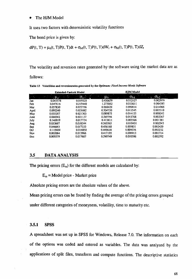
o The HJM Model

It uses two factors with deterministic volatility functions

The bond price is given by:

dP(t, T) = ~!,(t, T)P(t, T)dt + cr"(t, T)P(t, T)dW, + cr,,(t, T)P(t, T)dZ.

The volatility and reversion rates generated by the software using the market data arc as

follows:

Table 13 Volatilities and rfversloorates generated by tM Optimum: Fi.rtd /ru:omt Monis Softwrm:

Extended·V~kek Model HJM Model

Jm 0.043578 0.019525 0.456679 0.012127 0.002979

Fob 0.047616 0.219440 1.273052 0.01561 I 0.004585

MM 0.057830 0.022756 0.068429 0.009814 0.014066 April 0.090240 0.021682 0.504750 0.013545 0.003310 Moy 0.035287 0.021363 0.089875 0.014125 0.008242 J"re 0.066042 0.021137 0.569794 0.013768 0.003367 July 0.146819 0.017734 0.413811 0.005566 0.001381 A"g 0.053007 0.018244 0.565565 0.010401 0.002543 Sop 0.046683 0.017333 0.456168 0.009851 0.002420

"" 0.115609 0.014850 0.449618 0.009076 0.002232 N" 0.002084 0.013966 0.417195 0.006913 0.001714

"'' 0.005579 0.017607 0.590749 0.010586 0.002592

3.5 DATAANALYSIS

The pricing errors (Em) for the different models are calculated by:

Em = Model price - Market price

Absolute pricing errors are the absolute values of the above.

Mean pricing errors can be found by finding the average of the pricing errors grouped

under different categories of moneyness, volatility, time to maturity etc.

3.5.1 SPSS

A spreadsheet was set up in SPSS for Windows, Release 7 .0. The information on each

of the options was coded and entered as variables. The data was analyzed by the

applications of split files, transform and compute functions. The descriptive statistics

68

used to summarized the data were the mean, standard deviation and standard error.

Maximum and minimum were also iilcluded to assist data analysis. The parametric

statistics arc best represented by the mean, which shows the mathematical average of

the data.

3.5.2 Graphical Analysis

After the data has been grouped using SPSS, mean pricing errors and mean absolute

errors are plotted over time; against time to maturity, the degree to which options are in

or out-of·the-money.

3.5;3 Wilcoxon Signed Ranks Test

The Wilcoxon signed ranks test explains the sign of the difference between any pair and

rank the differences in order of absolute size. The null hypothesis is that the two paired

samples are from populations with the same medians and the same continuous

distribution. It makes no assumptions about the shapes of the distributions of the two

variables. The test takes into account information about the magnitude of differences

within pairs and gives more weight to pairs that show large difference than to pairs that

show small differences. Therefore, if the ranks having plus signs and negative signs

were summed respectively, the two sums should be about equal when H0 is true. But if

the sum of the positive ranks is very much different from the sum of the negative ranks,

it is inferred that the treatment of the two groups differs, and thus H0 is rejected.

69

3.5.4 OLS Regression and White's Corrections

To shed more light on the nature of the model's pattern of mispricing, a set of Ordinary

Least Square (OLS) regressions of the pricing errors on a constant, time to maturity, and

the degree to which the options were in- or out-of-the-money were performed. The

regressions were run for all the call futures options. This test examines whether the error

variance is affected by any of the regressors, their squares or their cross-products. It

tests specifically whether or not any heteroskedasticity present causes the variance­

covariance matrix of the OLS estimator to differ from its usual formula.

Four regression models were used:

R;..a,+ TIMy, +MONy,+E,

R,. a.+ TTMy, + MONy, + e,

R,.a.,+ TIMy, +MONy,+E.o

R.. a.+ TIMy, + MONy, +E.!

where

Ra.R..Ra.R. represents the pricing errors of the Black model, the Asay model, the

Extended-Vasicek model and the HJM model respectively. TIM is time to

maturity; MON is moneyness.

I did consider including a factor representing the option delta, which is the rate of

change of the option premium with respect to movements in the underlying futures

price. This is provided by the SFE based on the Asay Model but there seemed to he an

element of circularity involving in applying this, given that both the Black and Asay

model have similar constructions. The SFE also provides an estimate of volatility,

70

which again is an implied volatility from the Asay model. Similar concerns lead me to

reject its' use also.

71

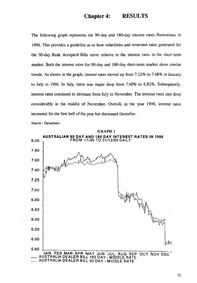
Chapter 4: RESULTS

The following graph represents the 90-day and 180-day interest rates nuctuations in

1996. This provides a guideline as to how volatilities and reversion rates generated for

the 90-day Bank Accepted Bills move relative to the interest rates in the short-term

market. Both the interest rates for 90-day and 180-day short-tenn market show similar

trends. As shown in the graph, interest rates moved up from 7.22% to 7.68% in January

to July in 1996. In July, there was major drop from 7.60% to 6.82%. Subsequently,

interest rates continued to decrease from July to November. The interest rates also drop

considerably in the middle of November. Overall, in the year 1996, interest rates

increased for the first half of the year but decreased thereafter.

Source : Datastream

GRAPH I

AUSTRALIAN 90 DAY AND 180 DAY INTEREST RATES IN 1996 8.00 FROM 111196 TO 31112196 DAILY

7.80

7.60

7.40

7.20

7.00

6.80

6.60

6.40

6.20

6.00

5.80 JAN FEB MAR APR 'MAY JUN JUL AUG SEP OCT NOV DEC

-AUSTRALIA DEALER BILL 180 DAY- MIDDLE RATE ......... AUSTRALIA DEALER BILL 90 DAY- MIDDLE RATE

72

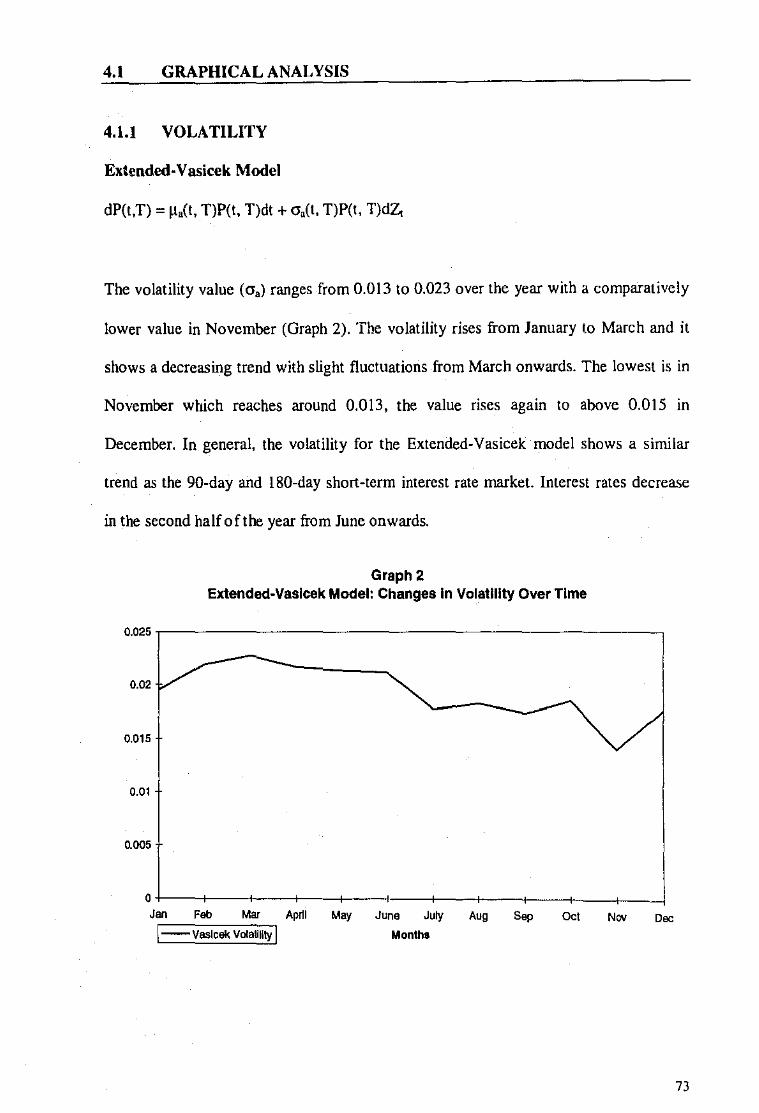
4.1 GRAPHICAL ANALYSIS

4.1.1 VOLATILITY

Extended· Vasicek Model

dP(t,T) = ~,(t, T)P(t, T)dt + cr,(t. T)P(t. T)dZ,

The volatility value (O'a) ranges from 0.013 to 0.023 over the year with a comparatively

lower value in November (Graph 2). The volatility rises from January lo March and it

shows a decreasing trend with slight fluctuations from March onwards. The lowest is in

November which reaches around 0.013, the value rises again to above 0.015 in

December. In general, the volatility for the Extended-Vasicek model shows a similar

trend as the 90-day and 180-day short-tenn interest rate market. Interest rates decrease

in the second half oft he year from June onwards.

Graph 2 Extended-Vasicek Model: Changes In Volatility Over Time

0.025,--------------------------~

0.02 v---------~

O.D15

0.01

0005

0~--r---~~---+--~---~--~--~--+---r--­- ~ ~ ~ - ~ - ~ - Oot Nw Doc

1-Vaslcel< Volatility I Months

73

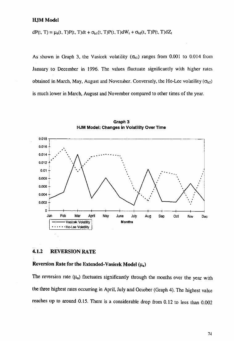
HJMModel

dP(t, T) = ~,(t, T)P(t, T)dt + cr., 1(t, T)P(t, T)dW, + cr,2(t, T)P(t, T)dZ,

As shown in Graph 3, the Vasicek volatility (O'bJ) ranges from 0.001 to 0.014 from

January to December in 1996. The values fluctuate significantly with higher rates

obtained in March, May, August and Noveruber. Conversely, the Ho-Lcc volatility (crb2)

is much lower in March, August and November compared to other times of the year.

Graph 3 HJM Model: Changes In Volatility Over Time

0.018

0.016 ' ..

0.014 ... ..... -. . ' 0.012

0.01 ... . ., 0.008

0.006 ' ' ' .

0.004 ' '• .

0.002 " . 0

Jan Feb Mar April May June Ju~ Aug Sop Oct N"' Doc

---Vasicek Volatility Months • • • • • • Ho-Lee Volatility

4.1.2 REVERSION RATE

Reversion Rate for the Extended-Vasicek Model (~)

The reversion rate (~) fluctuates significantly through the months over the year with

the three highest rates occurring in April, July and Ocwher (Graph 4). The highest value

reaches up to around 0.15. There is a considerable drop from 0.12 to less than 0.002

74

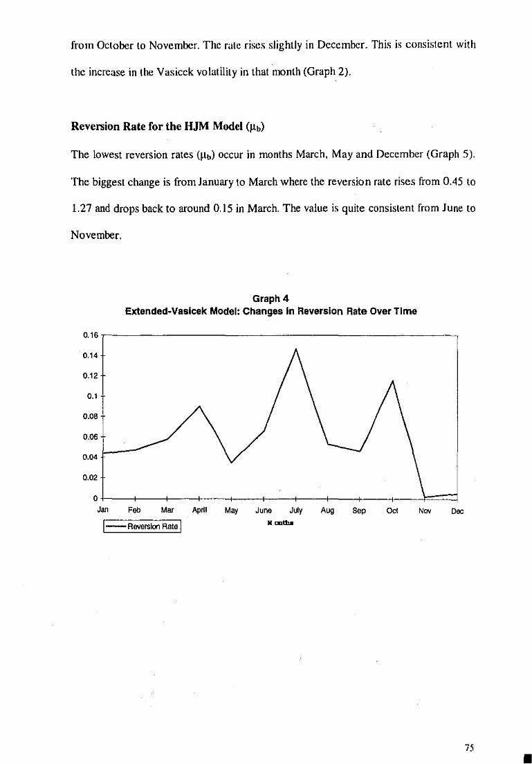
from October to November. The rate rises slightly in December. This is consistent with

the increase in the Vasicek volatilily in that month (Graph 2).

Reversion Rate for the HJM Model (flb)

The lowest reversion rates (J.lb) occur in months March, May and December (Graph 5).

The biggest change is from January to March where the reversion rate rises from 0.45 to

1.27 and drops back to around 0.15 in March. The value is quite consistent from June to

November.

Graph 4 Extended-Vasicek Model: Changes In Reversion Rate Over Time

0.16

0.14

0.12

0.1

0.08

0.06

0.04

0.02

0

'"' Feb M"' April May June July Aug Sep Ool Doc

1-Reversion Rate l ·~-

75 •

1.2

0.8

0.6

0.4

0.2

Graph 5 HJM Model: Changes in Reversion Rate Over Time

0 +---f----+------+----4----+-----+----+----+---+-----------,r----,

Jan Feb Mar April May June July Aug Sep Oct Nov Dec

\--Reversion Rate I Months

4.2 PRICING DEVIATIONS

4.2.1 MONEYNESS

Black Model and Asay Model

The manner in which pricing error changes for the four models when the options are

grouped into in-the-money, at-the-money and out-of-the-money' is illustrated in Graphs

6 & 7. The graphs are plotted using data shown in Table A. l & A.2 in the Appendices.

All mean pricing errors for the Black and Asay models are positive. As shown in Graph

6, the mean pricing error for both models increases as the value of the 'futures price -

strike price' increases. However, the Asay model shows a higher mean pricing error.

1The range of pricing error for different option categories: In-the-money options - (Futures Price - Strike Price)> 0.02 At-the-money options - -0.02 :5 (Futures Price - Strike Price) :5 0.02 Out-of-the-money options: - (Futures Price - Strike Price) < 0.02 The categories are chosen to make sure the at-the-money options have a small of difference between the futures price and the strike price.

76

Tenn Structure Models

The comparison of the mean absolute pncmg error between the Extended-Vasicek

model and the HJM model shows that the absolute error is considerably smaller for the

HJM model (Graph 7). This supports the fact that the HJM model is a relatively better

model to use. As illustrated in Graph 7, the HJM model overprices at-the-money options

but underprices both in-the-money and out-of-the-money options. Contrarily, the

Extended-Vasicek model overprices options in all categories.

a, :, iii > li .lO: .. IQ ::E ' a, :, iii > "ii '& ::E

a, :,

14

12

10

8

6

4

2

0

0.3

0.25

iii 0.2 > 1 la 0.15 ::E ' a,

.2 0.1 IQ > "ii -go.os ::E

0

-0.05

Graph 6 Mean Pricing Error by Moneyness: Black Model and ASAY Model

In-the-money

• Mean Pricing Error: Black

D Mean Pricing Error: ASAY

At-the-money

Moneyness

Graph 7

Out-of-the-money

Comparison of Pricing Errors for Extended-Vaslcek model and HJM model

Moneyness

• Absolute Mean Pricing Error Extended-Vasicek

• Absolute Mean Pricing Error: HJM

• Mean Pricing Error: Extended­Vasicek

DMean Pricing Error: HJM

77

Graphs 8, 9 & lO show how the mean pricing error and the mean absolute pricing error

change against the degree which the options arc in or out-of-the-money for the four

models. The degree to which the options are in or out-of-the-money is calculated using

the futures price minus the strike price. This is categorized into groups for analyzing the

pricing error.

Black Model and Asay Model

Graph 8 shows how the mean pricing error changes for the Black model and the Asay

model with different degrees of moneyness. Both models overprice the options. Overall,

the pricing error decreases as moneyness increases. The Asay model creates a higher

pricing error but the difference in error between the two models also decreases when

moneyness increases. The pricing errors decrease with an increasing rate from category

1.6 to 2.5 onwards.

Graph 8 Mean Pricing Error: Black Model and Asay Model

16~-----------------------------------------------------,

i 10 ~

6

... . . . . . . . -

.. 14 •••• . .. . . . . --.

-~------~:-~·~-~~~ ... . . -. . . 6 '

I 4

2

0~---+----+---~----~--~----~----~--~ <-3.5 ·3.6 to -2.5 ·2.6to ·1.5 -1.6 to ·0.5 ·0.6to 1.5 1.6 to 2.5 2.6 to 3.5 3.6to 4.5 4.6 to 5.5

Moneyneas

I ...... ::~I

Tenn Structure Models

From Graph 9, it can be seen that the Extended~ Vasicek model underpriccs deep in-the-

money options with moneyness 2.6 to 5.5 but overprices the other categories. Mean

pricing error increases from category <-3.5 to ranges -1.6 to -0.5 then decreases again

from -0.6 to 2.5 onwards. The HJM model overprices deep out-of-the-money options

but underprices most of the options in other ranges of moneyness. Mean pricing c:ror

decrease significantly for deep in-the-money options (from ranges I .6 to 2.5 onwards).

0.25

0.2

~ ~ 0.15

! 0.1

' • .2 0.05 ~

Graph 9 Mean Pricing Error by Moneyness: Extended-Vasicek model and HJM

model

·~~--~-~-~--~-~-~---~~----~----~----,-----~~--------~ -3.6 to -2.s -2~5·t; •• i .5 · :, :01o ·-o.s · ·.o.6 io·, ~s- • • • · • • • <· ,5 3.610 4.5 4.6 to 5.5

-0.05 ·-·"">.---

-0.1

Moneyness

I Extended-Vaslcek I • • • • • ·HJM

Looking at the mean absolute pricing error in Graph 10, it shows that the mean absolute

pricing error decreases significantly when using the Extended-Vasicek model for in-the-

money options from category -0.6 to 1.5 onwards. There is not much difference in error

between the two models for deep in-the-money options. Only in the ranges 2.6 to 3.5

does the HJM model have a higher mean absolute pricing error. Moreover, there is a

considerable decrease in mean absolute pricing error using the HJM model for at-the-

79

money and outRof-thc-money options. Overall, there is a general increase in trend for

mean absolute pricing errors as moncyncss increases up to category R0.6 to 1.5.

Graph 10 Mean Absolute Pricing Error by Moneyness:

Extended-Vasicek model and HJM model 0.25 ~---------------------

!l 0.2

:l! ~ 0.15 :!! ' ~ ~ 0.1

I 0.05

. . .. ' . '

ot---~--~----+---~--~----,---~--~ <·3,5 -3.61o -2.5 ·2.61o ·1.5 ·1.61o ·0.5 -0.6 to 1.5 1.6 to 2.5 2.6 to 3.5 3.6to 4.5 4.6 to 5.5

I Extended· Vasicek I Moneyness

_ · · · · ·HJM _

4.2.2 TIME TO MATURITY

Graphs 11 - 19 describe the change in mean pricing error and mean absolute pricing

error as time to maturity increases for in-thr-money, at-the-money and out-of-the-

money options for the four models. Information on data involved are presented the

Table A.3 in the Appendices. Graph 11 & 12 are the mean pricing error for the four

models when all options are grouped together. Graph 11 demonstrates that as time to

maturity increases, the mean pricing error and mean absolute pricing error increases for

both the Black model and the Asay model. Graph 12 shows that as time to maturity

increases, the mean pricing error for the Extended-Vasicek model on average increase

while that for the HJM model decreases. The graphs also show that the pricing error

80

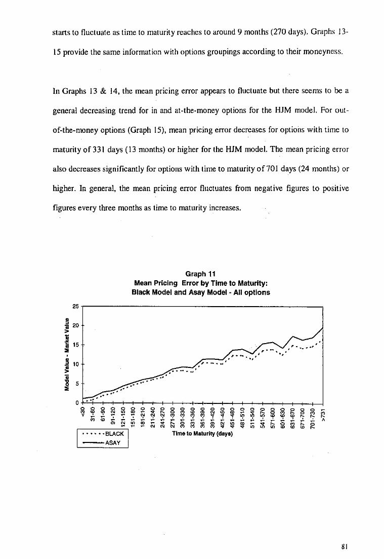
starts to fluctuate as time to maturity reaches to around 9 months (270 days). Graphs 13-

15 provide the same information with options groupings according to their moncyncss.

In Graphs 13 & 14, the mean pricing error appears to fluctuate but there seems to be a

general decreasing trend for in and at-the-money options for the H.JM model. For out-

of-the-money options (Graph 15), mean pricing error decreases for options with time to

maturity of 331 days ( 13 months) or higher for the HJM model. The mean pricing error

also decreases significantly for options with time to maturity of701 days (24 months) or

higher. In general, the mean pricing error fluctuates from negative figures to positive

figures every three months as time to maturity increases.

Graph 11 Mean Pricing Error by Time to Maturity:

Black Model and Asay Model -AU options

25r---------------------------------------------~

• .: 20 !!

115

0 •••

g g 2 g ~ 0 0 0 0

v ~ ~ ~ ~ ~ ~ ~ ~ w <0 ;;; c;:j ... .... .... ...

,----;;;-=0:..,... ~ ~ c;:j C1:i

•••• --BLACK I ASAY .

, --... ______ :--__ -_--:, . ,. .... . ,. ..... .

• •

81

Graph 12 Mean Pricing Error by Time to Maturity: Extended· Vasicek Model and

HJM Model • All options

0.4,------------------------, ~ 0.3 :!:! tl 0.2

~ ""' 0.1

'. . .. • '. . . . -0.3 .I_ ____________________ ___J

~ ~ ~ ~ ~ ~ ~ ~ ~ M tO ..... .... .... .... .... .... m~~~N~

g 0 0 g 0 0 0 0 0 g g 0 g g 0 -M w N ~

~ - ~ M M M

"! "! "! "! y y ~ ~ ~ ~ ~ ~ ~ ~

!i 0 iii ;;; ;; ~ ~ ~ - ~ ~ 0 10 ~ ~ h

M M M ~ ~ w w w

I Extended-Vaslcek I • • • • • ·HJM

Time to Maturity (days)

The mean absolute pricing errors for the four models have similar trends to those of the

mean pricing errors (Graphs 16-19). They clearly show the overall magnitude of the

fluctuation. Graph 16 demonstrate that there is a general increasing trend for the mean

absolute pricing error for the term structure models as time to maturity increases.

Graph 13 Mean Prlclng Error by Time to Maturity:

Extended-Vasicek Model and HJM Model- In-the-money options

0.3,---------------------,

~ :: 11 ~

0.25"

0.2

0.15

0.1

" • 0.05

~ :: -0.05

I -o.1

" -0.15

.. .. . . - ... . •

~--Extended-Vas leek I ······HJM

. . . ..

g 0 0 g 0

~ 0

::l w N ~ "! "! "! y - 0 - - ;; ~ ~ ~ ::l w

M M M • Time to Maturity (days)

• ' . . .. ..

' . .. . ... ..

0 0 0 g 0 0 8 0 M - ~ ~ !? 19 I? ~ "? '\' ~ ~ - - ~ - 0 10 - 0 ~ ;;; I;; ~ w w ~

82

~ <

30

31-6

0

' '

61-9

0 :o

om

~ ..

;:: !

91

·120

~

121-

150

~ 15

1-18

0

" 18

1-21

0 ~

211-

240

241-

270

...

271-

300

i 30

1-33

0

; 33

1-36

0

2-36

1-39

0 " ~ 3

91-4

20

i 42

1-45

0 ~

.!!..

451-

480

481-

510

511-

540

541-

570

571-

600

601-

630

631-

670

671-

700

701-

730

>731

~

·~

Mo

del

Va

lue

-M

arke

t V

alu

e

e ~

<> c:

~ ~

, -0

~

•

-.•

, '

, m

~ " I i n ;;

~;

" ..

,..,

;!::

S

0 '0

a.~

.. - -!!.

.. :

s

""'

"-m

~~C)

'-0

"

:=:--

.-!

3: ~ :

:r o

-<­

"--"

' !!

!.3

'

.. o

c;

S;~;

'

" 0

--:

"c:;

-"

:s--

'P~

3 ..

0 :s ~ .g 0 :s ..

<> ~

<3

0 I

• 0

c ~

;:: ! ~

61-9

0

~ " 12

1-15

0

~

181-

210

241-

270

::! i

301-

330

;; " ~ 3

61-3

90

~ i

421-

450

:;_ 48

1-51

0

541-

570

601-

630

671-

700

>731

<> N ' M

od

el V

alu

e-

Mar

ket

Val

ue

<> ,

:;; ,

0 ~

' ~

~ 0

0 ~

1..n

~ :s "- ~ <

!Jl ;;!

; -

.. n

" ~:s

;~:'

0 0

::!.

a.!!

. ~~

!!l m

Q.~C)

_o

"

~""'

'-C

' '0

;;!

; '<

,.

;~;-<­

o-"

' ..

_3

" .. -- ' 0 ~== -=

:s--

'1' !;

3~

0 ..

:s

~ .g - g ..

't

. 2: ~

;:: ~ §: f

I Mo

de

l Va

lue

-M

ark

et

Va

lue

I

(;

p ~

p 0

01

....

.. 0

11

\J

<30

..

3H

i0

61

-90

91-1

20

121-

150

151-

180

181·

210

2H

-24

0

241·

270

....

271·

300

f 3

01

·33

0

~ 33

1·36

0

~ 3

61

-39

0

~ 3

91-4

20

i 42

1-45

0 ~

.!!.

451-

480

481-

510

511·

540

541-

570

571-

600

601-

630

631-

670

671-

700

. ' • '

<

•' •. ·. . ' ' .. •'

. .. •

• .

• . •

70

1-7

30

t .-

:: _

__

__

__

_ _

>731

-

'

0 N '"

i " D. ";=

: ~l

l .,

" !!

.)>

n.

,. ....

"'o

;=

:;:

o­

c.<>

.. ..

, -~

., -

" !!

. D

.:IC

) :c

co

D1 <-

m.,

;l

:'l:

:r

_o_

~~

... 0

.,.

D.>

e ~--~

~3

" .. ·-:To

'P

;c

3 a

0 "

" ~

.. - ... .:<

i ..

g ..

0

I Mo

del

Va

lue

-M

arke

t V

alu

e I

0 ~

~ 0

e 0 tll

0 "' 0 bl

<30 r-

---=

-+--

l--+

--+

---;

-""1

31

-60

61-9

0

91-1

20

~ ~

;:: ~ ! 12

1-15

0

151-

180

181-

210

211-

240

241-

270

-I

271-

300

i 30

1-33

0

~ 33

1-36

0

e-36

1-39

0

~ 3

91-4

20

i 42

1-45

0 ~

-45

1-48

0

481-

510

511-

540

541-

570

571-

600

601-

630

631-

670

671-

700

701-

730

•' • . . ' ' ... -

.- ----

>731

"-----------------~~------~

m

~;c

" l1

"'"

il.,.

. .,.

<

.,

.,

0 .,

--c:

n - .. .. .. .., ;=

:::!.

g_~C

) !!.

co

; .,

m,

" ~

::r

c.a ..

... ::~:~.,

.... .,.

;1:'

<

;c::

l 0

3

"'"

!!.c

; • ,.;c

=

a 0

" '0

::!,

<=

.:<

0 ..

" .,

Graph 18 Mean Absolute pricing error by Time to Maturity:

Extended· Vasicek Model and HJM Model ·At the money options

- 0.45.-----------------------, !: 0 .fo

~ O.JS <;; ~ 0.3 ~ ~ O.lS

_;, O.l , ~ 0.15

] 0.1 r.J1 ""' 0. OS

0 +-tJ..Otl.a,lJO,..--0

" " 0 • ' " •

0 0 . " " " ' ' " " " .

====="::;-::=" QJtxtended-Va•ieek .. ,. 0

' " ' " • "

0 0 0

" • • " " • ' ' ' " " " 0 • " " " •

Time to Maturity (days)

0

" • ' " • •

0

' • ' " • •

0

" • ' " 0 •

0 0

' ' " ~

As shown in Graphs 17 & 18, the HJM model leads to a lower pricing error for in- and

at-the-money options. For in-the-money options (Graph 17), mean absolute pricing

error increases as time to maturity increases. The error tends to be lower for shorHerm

(<90 days) and long-term (>600 days) at-the-money options when priced using the HJM

model (Graph 18). Graph 19 shows a similar trend to Graph 16 for out-of-the-money

options.

4.2.3 VOLATILITY

Black Model and Asay Model

The relationship between mean pricing error changes and different volatility ranges for

the Black model and the Asay model are presented in Graph 20. Mean pricing error

increases as volatility increases. The mean pricing error for the Asay model also

becomes higher compared to the Black model as volatility increases.

85 I

• , ~ ~

.!! -• "' • • .2 • > .. '8 "'

0.45

0.4

0.35

0.3

0.25

0.2

0.15

0.1

0.05

0

<00

Graph 19 Meah Absolute Pricing Error by Time to Maturity:

Extended~ Vasicek Model and HJM Model ~Out-of-the-money options

-... . -••

. . .. --. · ...... .

61· 121- 161· 241· 301- 361· 421· 481- 541- 601· 671· >731

oo 1~ 210 m • m • s1o m - ~

I Extanded.Vaslcek I • • • • • ·HJM

Time to Maturity (days)

Graph 20 Mean Pricing Error by Vola111lty: Black Mo•lel and Asay Model

20

18

• 16 ~

14 > s ~ 12 " • "' 10 • • .2 8 ~

'

.. 6 '8 " 4

2

0 0.05-0.1 0.11-0.15 0.16·0.2 0.21·0.25 0.26-0.3 0.31·0.35 0.36·0.4 0.41-0.45

Black VolatiUty

······ASAY

Tenn Structure Models

The mean pricing error for at-the-money options shows a completely different trend for the two term

structure models. The Extended-Vasicek model shows that pricing error is negative for options with

volatility values of less than 0.16 (Graph 21 ). Above 0.16, pricing error tends to be positive. The model

86 I

overprices the options above this point and pncmg error increases as volatility

increases. The HJM model only overprices options in volatility ranges 0.21-0.25 and

0.41-0.45. The model underpriccs options in other categories.

o.a

0.25

• 0.2

~ 0.15 ]1 • 0.1 • "' 0

• 0.05 , :i! .. 0

1l ::::& ·0.05

·0.1

Graph 21 Mean Pricing Error by Volatility: Ex1ended-Vaslcek Model and HJM

Model

...... --. - . . . . ..... .

....

i

..... · · ·1

·0.15 J.__ __________________________ _j

0.05·0.1 0.11·0.15 0.16-0.2 0.21·0.25 0.26-0.3 0.31-0.35 0.36·0.4 0.41-0.45

Volatility ~ Mean Extendad-Vaslcek I ··-·--Mean HJM

The absolute pricing error in Graph 22 shows that the error is lower especially for

options in categories 0.05-0.1 and 0.41-0.45 (deep in and out-of-the-money options).

The mean absolute pricing error is lower when the HJM model is used. Both term

structure models show approximately the same trend for volatility ranges from 0.05 to

0.35. With volatility values of 0.35 or above, mean absolute pricing error for the HJM

model decreases while that for the Extended-Vasicek model increases. The difference in

error between the two models then becomes larger.

87

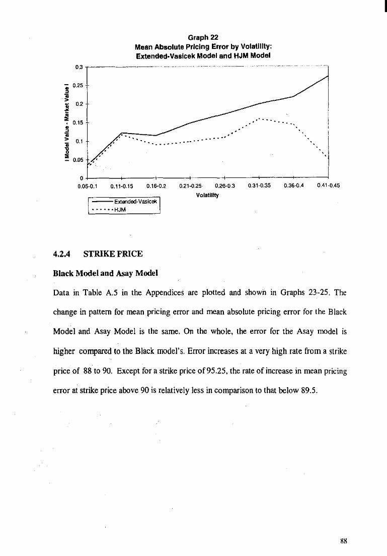
Graph 22 Mean Absolute Pricing Error by Volatility: Extended-Vasicek Model and HJM Model

0.3 ----------- --- -··· ------· -------

• 0.25 , ~ j 0.2

~ ' 0.15 ~ ;! ~ 0.1

~ 0.05

. . . . . .. . . . ... . . . . . . . ..... ...

.... ... . ·- '

l . ' • I .I 0~----+-----+-----+-----+-----~----~--~

0.05·0.1 0.11·0.15 0. 16·0.2 0.21·0.25 0.26-0.3 0.31-0.35 0.36-0.4 0.41-0.45

\ Extended.Vasicek I • • • • • • HJM

Volatility

4.2.4 STRIKE PRICE

Black Model and Asay Model

Data in Table A.5 in the Appendices are plotted and shown in Graphs 23-25. The

change in pattern for mean pricing error and mean absolute pricing error for the Black

Model and Asay Model is the same. On the whole, the error for the Asay model is

higher compared to the Black model's. Error increases at a very high rate from a strike

price of 88 to 90. Except for a strike price of 95.25, the rate of increase in mean pricing

error at strike price above 90 is relatively less in comparison to that below 89.5.

I

• 2 • > ~ ~ • • " ' • ~ > .. ~

"

• , ii > l • • " ' • 2 ~ ii ll "'

12

10

B

6

4

2

0 ~ •

0.25

0.2

0.15

0.1

o.os

0

-0.05

~

:8

. , ,

Graph 23 Mean Pricing Error: Black Model and Asay Model

Lf! ~ lfl ;; Sl Strike Price

. . . . . ...... . . .-·.·

Black

• • • • • ·ASAY

Graph 24 Mean Pricing Error by Strike Price: Extended-Vasicek MQdel and HJM

Model

~ ll'.o"""' ll'l"""""""<b ·--1/1-IQ tn"•". ;;·-·. Sl .•• -~-- .IQ ••• ~-- .IQ •• '!!2 . • ·~ • 0 ~ N M • - ~ ,. <0,. 01 0> (71 01 (J} OJ

'

-0.1 ~~~~~.~~~..,;;;d..,~--V~os;-,~,ek~~m~-~l~--;S~1t~lk=e~P~d:c~e-----------_J

_ • • • • • ·HJM _

I

89

Term Structure Model•

Graphs 24 & 25 show how mean pricing error and mean absolute pricing error chtmgc

as strike price increases. In Graph 24, it shows that the HJM model tends to underprice

all options with different strike prices. Mean pricing error fluctuates between 0 to ~0.1

with error between 0 to -0.05 above strike price 89.25. The Extcndcd-Vao;;icek model

overprices options with strike price of above 89.25 but underprices options with strike

prices below that point. Mean pricing error increases as strike price increases up to 92.5.

Thereafter, error tends to drop subsequently as strike price increases. This shows that

the HJM model gives a better approximation for pricing since the spread of the error is

of a lesser extent. As seen in Graph 25 for mean absolute pricing error, the HJM model

provides an overall lower absolute error in pricing. Moreover, as strike price increases,

the HJM model gives a substantially lower error compared to the Extended-Vasicek

model.

Graph 25 Mean Absolute Pricing Error by strike price:

Extended-Vasicek Model and HJM Model 0.25,----------------------------,

-• .2 0.2 ,: j :0 0.15 ,. • • -i 0.1 >

I 0.05

. .... .. .. . . .. ···-----· .. ____ _

Strike Price

'• ' • ·.

' ' . . . . ' .....

90

I

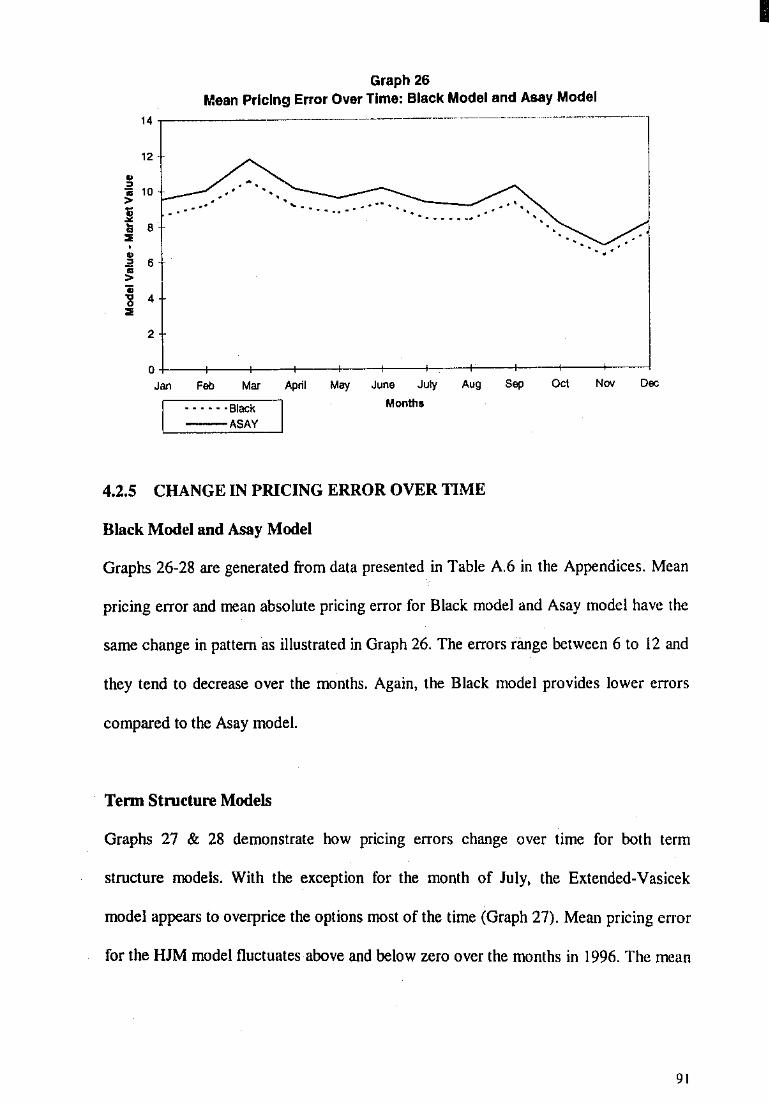
Graph 26 Mean Pricing Error Over Time: Black Model and Asay Model

14,------

12

... . . .

2

---~------- -~----~---·- --------------.-~----·-

. . .. . . ... ..

o+-~~~~-+~~~+-~~~~-+~-+-~+-~ - ~ - ~ -- - ~ - ~ - -• • · • • ·Black

ASAY

Months

4.2.5 CHANGE IN PRICING ERROR OVER TIME

Black Model and Asay Model

Graphs 26-28 are generated from data presented in Table A.6 in the Appendices. Mean

pricing error and mean absolute pricing error for Black model and Asay model have the

same change in pattern as illustrated in Graph 26. The errors range between 6 to 12 and

they tend to decrease over the months. Again, the Black model provides lower errors

compared to the Asay model.

Tenn Structure Models

Graphs 27 & 28 demonstrate how pricing errors change over time for both term

structure models. With the exception for the month of July, the Extended-Vasicek

model appears to overprice the options most of the time (Graph 27). Mean pricing error

for the HJM model fluctuates above and below zero over the months in 1996. The mean

91

I

absolute pricing error for HJM model is lower for all months except for July when the

Extended-Vasicek model underprices the options (Graph 28).

Graph 27 Mean Pricing Error Over Time: Exter.ded-Vaslcek Model and HJM

Model 0.4,-----·

0.3

! 0.2 .. . . ;:! 0.1

.. ... -· • ~

. . -. · . . • "

. . . . . Feb ..,,

A~r11 ... , June, . .

Graph 28 Mean Absolute Pricing Error: Extended-Vaslcek Model and HJM Model

0.4,---------------------------,

0.35

• ~ 0.3

j 0.25

~ ' 0.2 ] ~ 0.15

I .----·. ""' 0,1

0.05

.. . .. . . . . . ..

·.

' •' . · .

... ... 0~-~~--+--+·-~-~-+--+--r---~~ J ... Feb Mar April May June July Aug Sep Oot Dec

Months L Extended-Vaslcek ······HJM

92

I

4.3 WILCOXON SIGNED RANKS TESTS

Results from the use of the Wilcoxon Signed Ranks Test in testing pricing errors and

absolute pricing errors for the three models arc given in Tables 14, 15, 16 &17. The sign

tests report the mean rank, the sum of the ranks and the test statistics for mean and

absolute pricing errors. The test statistics arc based on the ranks of the absolute value

difference between the two variables. The pricing errors and the absolute pricing errors

generated by different models are grouped by pairs in order to test for their significance.

2-tailed tests are used to compare the data. In Tables 14, 15, 16 &17, the mean and

mean absolute pricing errors of the Black Model, the Extended-Vasicek Model and the

HJM Model are shown to be significantly different from each other at the 0.05 level.

Therefore, the null hypothesis that the pricing errors and the absolute pricing errors of

the four models have the same distribution can be rejected.

Table 14 & 15 analyze the pricing error far the four models, they shaw that the number

of the negative ranks is greater than the number of positive ranks when: 1) Black Error­

Asay Error; 2)Vasicek Error- Black Error; 3) HJM Error- Vasicek Error.

This demonstrates that:

I) Black Error< Asay Error;

2)Vasicek Error< Black Error

3) EJM Error< Vasicek Error.

Similarly, by looking at Tables 16 & 17, they prove that:

I) Absolute Black Error< Absolute Asay Error;

2) Absolute Vasicek Error< Absolute Black Error

3) Absolute HJM Error< Absolute Vasicek Error.

93

I

Table 14

Tables 14 & 15 show the nonparametric statistics for the pricing error for the Black model, Asay model, Extended-Vasicek model and HJM model for call options on 90-Day Bank Accepted Bill Futures.

Black Error - Asay Error

Vasicek Error - Black Error

a. Black Error < Asay Error

b. Black Error > Asay Error

c. Asay Error= Black Error

d. Vasicek Error< Black Error

e. Vasicek Error> Black Error

f. Black Error= Vasicek Error

Ranks

Negative Ranks

Positive Ranks

Ties

Total

Negative Ranks

Positive Ranks

Ties

Total

Test Statistics!

N a

2097

ob

oc 2097

2075 d

228

at 2097

Black Error - Asay Error Vasicek Error - Black Error z -39.663° Asymp. Sig. .000 (2-tailed)

a. Wilcoxon Signed Ranks Test

b. Based on positive ranks.

Note: Pricing Error = Model Price - Actual Price Absolute Pricing Error= I Model Price - Actual Price I Black Error= Pricing Error for the Black Model Asay Error= Pricing Error for the Asay Model

-39.6500

.000

Vasicek Error= Pricing Error for the Extended-Vasicek Model HJM Error = Pricing Error for the HJM Model Abs Black Error= Absolute Pricing Error for the Black Model Abs Asay Error= Absolute Pricing Error for the Asay Model

Mean Rank

1049.00

.00

1059.95

16.55

Abs Vasicek Error= Absolute Pricing Error for the Extended-Vasicek Model Abs HJM Error= Absolute Pricing Error for the HJM Model

Sum of Ranks

2199753

.00

2199389

364.00

94

Table 15

Ranks

N a Vasicek Error - HJM Error Negative

Ranks 340

b Positive Ranks 1753

Ties 4c

Total 2097

a. Vasicek Error < HJM Error

b. Vasicek Error > HJM Error

c. HJM Error = Vasicek Error

Test Statistics a

Vasicek Error - HJM Error z Asymp. Sig. (2-tailed)

a. Wilcoxon Signed Ranks Test

b. Based on negative ranks.

Note: Pricing Error = Model Price - Actual Price Absolute Pricing Error= I Model Price - Actual Price I Black Error= Pricing Error for the Black Model Asay Error= Pricing Error for the Asay Model

-36.808°

.000

Vasicek Error= Pricing Error for the Extended-Vasicek Model HJM Error= Pricing Error for the HJM Model Abs Black Error= Absolute Pricing Error for the Black Model Abs Asay Error = Absolute Pricing Error for the Asay Model

Mean Rank

229.07

1205.64

Abs Vasicek Error= Absolute Pricing Error for the Extended-Vasicek Model Abs HJM Error= Absolute Pricing Error for the HJM Model

Sum of Ranks

77883.50

2113488

95

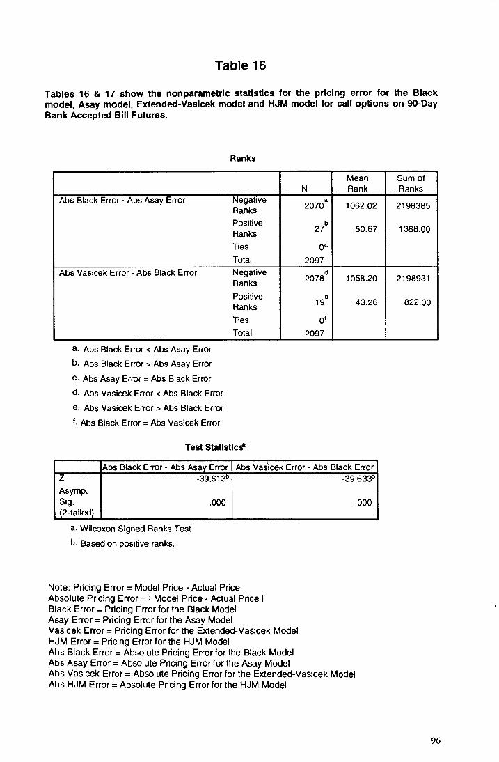
Table 16

Tables 16 & 17 show the nonparametric statistics for the pricing error for the Black model, Asay model, Extended-Vasicek model and HJM model for call options on 90-Day Bank Accepted Bill Futures.

Abs Black Error - Abs Asay Error

Abs Vasicek Error - Abs Black Error

a. Abs Black Error < Abs Asay Error

b. Abs Black Error > Abs Asay Error

c. Abs Asay Error = Abs Black Error

d. Abs Vasicek Error < Abs Black Error

e. Abs Vasicek Error> Abs Black Error

f. Abs Black Error= Abs Vasicek Error

Ranks

Negative Ranks Positive Ranks

Ties

Total

Negative Ranks

Positive Ranks

Ties

Total

Test Statistics&

Mean N Rank

a 2070 1062.02

27b 50.67

oc 2097

2078d 1058.20

e 19 43.26

o' 2097

Abs Black Error - Abs Asay Error Abs Vasicek Error - Abs Black Error z -39.613° -39.633° Asymp. Sig. .000 (2-tailed)

a. Wilcoxon Signed Ranks Test

b. Based on positive ranks.

Note: Pricing Error = Model Price - Actual Price Absolute Pricing Error = I Model Price - Actual Price I Black Error= Pricing Error for the Black Model Asay Error = Pricing Error for the Asay Model Vasicek Error= Pricing Error for the Extended-Vasicek Model HJM Error= Pricing Error for the HJM Model Abs Black Error = Absolute Pricing Error for the Black Model Abs Asay Error= Absolute Pricing Error for the Asay Model Abs Vasicek Error= Absolute Pricing Error for the Extended-Vasicek Model Abs HJM Error= Absolute Pricing Error for the HJM Model

.000

Sum of Ranks

2198385

1368.00

2198931

822.00

96

Table 17

Ranks

Mean N Rank

Abs Vasicek Error - Abs HJM Error Negative a

Ranks 543 856.06

Positive b

Ranks 1549 1113.26

Ties 5c

Total 2097

a. Abs Vasicek Error < Abs HJM Error

b. Abs Vasicek Error > Abs HJm Error

c. Abs HJM Error = Abs Vasicek Error

Test Statistics a

Abs Vasicek Error - Abs HJM Error z Asymp. Sig. (2-tailed)

a. Wilcoxon Signed Ranks Test

b. Based on negative ranks.

Note: Pricing Error = Model Price - Actual Price Absolute Pricing Error= I Model Price - Actual Price I Black Error= Pricing Error for the Black Model Asay Error= Pricing Error for the Asay Model Vasicek Error= Pricing Error for the Extended-Yasicek Model HJM Error= Pricing Error for the HJM Model Abs Black Error= Absolute Pricing Error for the Black Model Abs Asay Error= Absolute Pricing Error for the Asay Model Abs Vasicek Error= Absolute Pricing Error for the Extended-Vasicek Model Abs HJM Error= Absolute Pricing Error for the HJM Model

Overall results can be summarized by their direction of dominance:

• Mean Pricing Error

-22.793°

.000

Sum of Ranks

464840

1724438

Asay Model Error > Black Model Error> Extended-Vasicek Model Error > HJM Model

Error

97

• Mean Absolute Pricing Error

Asay Model Error> Black Model Error> Extended-Vasicek Model Error> HJM Model

Error

The Wilcoxon Signed Ranks tests reveal that the HJM model is the best pricing model

to use. Evidence shows that the term structure models have considerably lower mean

and mean absolute pricing error. However, as discussed previously, data on options and

the underlying stock may not be taken at the same time and the market can appear to be

nonsynchronous. This can affect the results generated.

4.4 THE OLS REGRESSIONS AND WHITE'S ADJUSTMENTS

Tables 18-21 show the Ordinary Least Square (OLS) Regressions for mean pricing error

for the Black Model, the Asay Model, the Extended-Vasicek Model and the HJM

Model. Mean pricing error is chosen as the dependent variable as the direction of error

can be involved in the analysis. The pricing error was regressed on time to maturity and

the degree to which options were in and out-of-the-money. The regressions were run for

all the call options throughout the period. R-squares indicate the percentage of error

variation explained by the independent variables. The correlation matrices of different

variables are also given in the tables. They give an idea of how much the different

variables relate to one another.

Black Model

The OLS Regression for the Black Model is shown in Table 18. Both the variables

time-to-maturity and moneyness are statistically significant at the 0.05 level and are

able to explain the error change. The coefficients in the regression have a t-value of

98

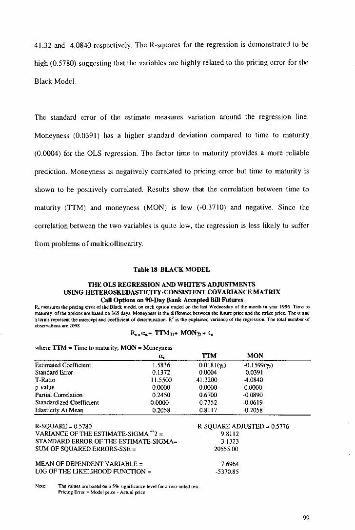
41.32 and -4.0840 respectively. The R-squares for the regression is demonstrated to be

high (0.5780) suggesting that the variables are highly related to the pricing error for the

Black Model.

The standard error of the estimate measures variation around the regression line.

Moneyness (0.0391) has a higher standard deviation compared to time to maturity

(0.0004) for the OLS regression. The factor time to maturity provides a more reliable

prediction. Moneyness is negatively correlated to pricing error but time to maturity is

shown to be positively correlated. Results show that the correlation between time to

maturity (TIM) and moneyness (MON) is low (-0.3710) and negative. Since the

correlation between the two variables is quite low, the regression is less likely to suffer

from problems of multicollinearity.

Table 18 BLACK MODEL

THE OLS REGRESSION AND WHITE'S ADJUSTMENTS USING HETEROSKEDASTICITY-CONSISTENT COVARIANCE MA TRIX

Call Options on 90-Day Bank Accepted Bill Futures R, measures the pricing error of the Black model on each option traded on the last Wednesday of the month in year 1996. Time to maturity of the options are based on 365 days. Moneyness is the difference between the future price and the strike price. The a and y terms represent the intercept and coefficient of determination. R2 is the explained variance of the regression. The total number of observations are 209 8.

where TTM = Time to maturity; MON = Moneyness

ex. Estimated Coefficient Standard Error T-Ratio p-value Partial Correlation Standardized Coefficient Elasticity At Mean

R-SQUARE = 0.5780

1.5836 0.1372 11.5500 0.0000 0.2450

0.0000 0.2058

VARIANCE OF THE ESTIMATE-SIGMA .. 2 = STANDARD ERROR OF THE ESTIMATE-SIGMA= SUM OF SQUARED ERRORS-SSE =

MEAN OF DEPENDENT VARIABLE = LOG OF THE LIKELIHOOD FUNCTION =

TIM 0.018l(y1)

0.0004 41.3200 0.0000 0.6700 0.7352 0.8117

MON -0.1599( Yz) 0.0391

-4.0840 0.0000 -0.0890 -0.0619 -0.2058

R-SQUARE ADJUSTED = 0.5776 9.8112 3.1323

20555.00

7.6964 -5370.85

Note: The values are based on a 5% significance level for a two-tailed test. Pricing Error = Model price - Actual price

99

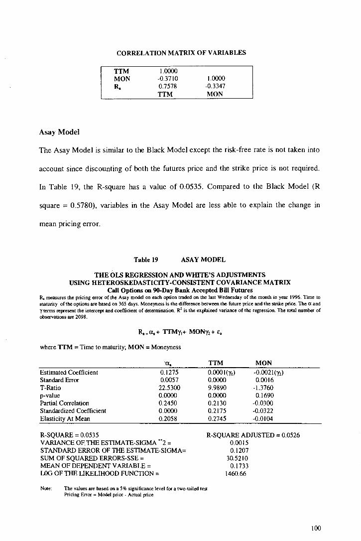
Asay Model

CORRELATION MATRIX OF VARIABLES

TTM MON R.

1.0000 -0.3710 0.7578 TTM

1.0000 -0.3347 MON

The Asay Model is similar to the Black Model except the risk-free rate is not taken into

account since discounting of both the futures price and the strike price is not required.

In Table 19, the R-square has a value of 0.0535. Compared to the Black Model (R

square = 0.5780), variables in the Asay Model are less able to explain the change m

mean pricing error.

Table 19 ASAY MODEL

THE OLS REGRESSION AND WHITE'S ADJUSTMENTS USING HETEROSKEDASTICITY -CONSISTENT COVARIANCE MA TRIX

Call Options on 90-Day Bank Accepted Bill Futures R. measures the pricing error of the Asay model on each option traded on the last Wednesday of the month in year 1996. Time to maturity of the options are based on 365 days. Moneyness is the difference between the future price and the strike price. The a and y terms represent the intercept and coefficient of determination. R2 is the explained variance of the regression. The total number of observations are 2098.

where TTM = Time to maturity; MON = Moneyness

Estimated Coefficient Standard Error T-Ratio p-value Partial Correlation Standardized Coefficient Elasticity At Mean

R-SQUARE = 0.0535

0.1275 0.0057

22.5300 0.0000 0.2450 0.0000 0.2058

VARIANCE OF THE ESTIMATE-SIGMA .. 2 = STANDARD ERROR OF THE ESTIMATE-SIGMA= SUM OF SQUARED ERRORS-SSE = MEAN OF DEPENDENT VARIABLE = LOG OF THE LIKELIHOOD FUNCTION =

TTM O.OOOl(Yt) 0.0000 9.9890 0.0000 0.2130 0.2175 0.2745

MON -0.002l(y2) 0.0016

-1.3760 0.1690

-0.0300 -0.0322 -0.0104

R-SQUARE ADJUSTED = 0.0526 0.0015 0.1207

30.5210 0.1733

1460.66

Note: The values are based on a 5% significance level for a two-tailed test. Pricing Error = Model price - Actual price

I 00

CORRELATION MATRIX OF VARIABLES

TTM MON R.

1.0000 -0.3710 0.7578

1.0000 -0.3347

TTM MON

All variables are statistically significant at the 0.05 level. T-value for time to maturity is

9.9890 while that for moneyness is -1.3760. The standard error for time to maturity is

again lower compared to moneyness. Similar to results presented in the Black Model,

moneyness is negative correlated to the pricing error. The figures for both the estimated

(-0.0021) and standardized coefficient (-0.0322) for moneyness are negative. Therefore,

the higher the degree of moneyness, the lower the pricing error. This is also consistent

with the result in Graph 8.

The variable time to maturity is positively correlated to pricing error. Partial correlation

also suggests that time to maturity can better explain pricing error (0.2130 for TIM and

-0.0300 for MON).

The Extended Vasicek Model

Table 20 presents the OLS regression with the mean pricing' error of the Extended­

V asicek Model as the dependent variable. The results inaicate that the values for the T­

ratio for all the variables are high and significant at the 0.05 level. The T-ratio for time

to maturity is very high (167 .2). This indicates that time to maturity is a crucial factor

that drives the mean pricing error. The T-Ratio for moneyness is also high (-20.11 ),

although not as significant as that for time to maturity. The variables also have a very

high correlation (shown by the R-square of 0.9429) with the mean pricing error. This

suggests that the factors successfully account for the change in pricing errors.

101

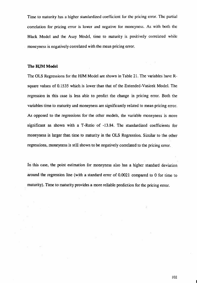
Time to maturity has a higher standardized coefficient fur the pricing error. The partial

correlation for pricing error is lower and negative for moncyncss. As with both the

Black Model and the Asay Model, time to maturity is positively correlated while

moneyness is negatively correlated with the mean pricing error.

The HJM Model

The OLS Regressions for the HJM Model are shown in Table 21. The variables haveR­

square values of 0.1535 which is lower than that of the Extended-Vasicek Model. The

regression in this case is less able to predict the change in pricing error. Both the

variables time to maturity and moneyness are significantly related to mean pricing error.

As opposed to the regressions for the other models, the variable moneyness is more

significant as shown with a T -Ratio of -13.84. The standardized coefficients for

moneyness is larger than time to maturity in the OLS Regression. Similar to the other

regressions, moneyness is still shown to be negatively correlated to the pricing error.

In this case, the point estimation for moneyness also has a higher standard deviation

around the regression line (with a standard error of 0.0021 compared to 0 for time to

maturity). Time to maturity provides a more reliable prediction for the pricing error.

102 I

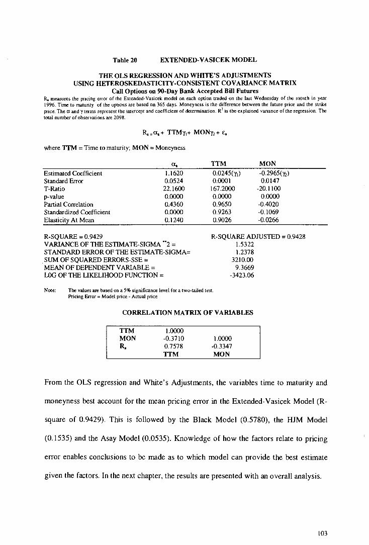
Table 20 EXTENDED-V ASICEK MODEL

THE OLS REGRESSION AND WHITE'S ADJUSTMENTS USING HETEROSKEDASTICITY-CONSISTENT COVARIANCE MATRIX

Call Options on 90-Day Banlc Accepted Bill Futures R, measures the pricing error of the Extended-Vasicek model on each option traded on the last Wednesday of the month in year 1996. Time to maturity of the options are based on 365 days. Moneyness is the difference between the future price and the strike price. The a and y terms represent the intercept and coefficient of determination. R2 is the explained variance of the regression. The total number of observations are 2098.

where TTM = Time to maturity; MON= Moneyness

Estimated Coefficient Standard Error T-Ratio p-value Partial Correlation Standardized Coefficient Elasticity At Mean

R-SQUARE = 0.9429

a. 1.1620 0.0524 22.1600 0.0000 0.4360 0.0000 0.1240

VARIANCE OF THE ESTIMATE-SIGMA .. 2 = STANDARD ERROR OF THE ESTIMATE-SIGMA= SUM OF SQUARED ERRORS-SSE = MEAN OF DEPENDENT VARIABLE = LOG OF THE LIKELIHOOD FUNCTION =

TTM 0.0245(y1) 0.000 I

167 .2000 0.0000 0.9650 0.9263 0.9026

MON -0.2965(y2) 0.0147

-20.1100 0.0000

-0.4020 -0.1069 -0.0266

R-SQUARE ADJUSTED= 0.9428 1.5322 1.2378

3210.00 9.3669

-3423.06

Note: The values are based on a 5% significance level for a two-tailed test. Pricing Error= Model price - Actual price

CORRELATION MATRIX OF VARIABLES

TTM MON R.

1.0000 -0.3710 0.7578 TTM

1.0000 -0.3347 MON

From the OLS regression and White's Adjustments, the variables time to maturity and

moneyness best account for the mean pricing error in the Extended-Vasicek Model (R­

square of 0.9429). This is followed by the Black Model (0.5780), the HJM Model

(0.1535) and the Asay Model (0.0535). Knowledge of how the factors relate to pricing

error enables conclusions to be made as to which model can provide the best estimate

given the factors. In the next chapter, the results are presented with an overall analysis.

103

Table 21 HJMMODEL

THE OLS REGRESSION AND WHITE'S ADJUSTMENTS USING HETEROSKEDASTICITY-CONSISTENT COVARIANCE MATRIX

Call Options on 90-Day Bank Accepted Bill Futures R. measures the pricing error of the I-UM model on each option traded on the last Wednesday of the month in year 1996. Time 10

maturity of the options are based on 365 days. Moneyness is the difference between the future price and the strike price. The a and y terms represent the intercept and coefficient of determination. R2 is the explained variance of the regression. The total number of observations are 2098.

where TTM = Time to maturity; MON= Moneyness

Estimated Coefficient Standard Error T-Ratio p-value Partial Correlation Standardized Coefficient Elasticity At Mean

R-SQUARE = 0.1535

a.. 0.0932

0.0077 12.1200 0.0000 0.2560 0.0000

0.7817

VARIANCE OF THE ESTIMATE-SIGMA ··2 = STANDARD ERROR OF THE ESTIMATE-SIGMA= SUM OF SQUARED ERRORS-SSE= MEAN OF DEPENDENf VARIABLE= LOG OF THE LIKELIHOOD FUNCTION =

TTM 0.0002(y1) 0.0000 7.3020 0.0000 0.1580 0.1609 0.4205

MON -0.0286(y2)

0.0021 -13.8400

0.0000 -0.2890 -0.3025 -0.2021

R-SQUARE ADJUSTED = 0.1527 0.0264 0.1626

55.3730 0.1192

835.822

Note: The values are based on a 5% significance level for a two-tailed test. Pricing Error= Model price - Actual price

CORRELATION MATRIX OF VARIABLES

TTM MON R.

l.0000 -0.3710 0.7578 TTM

1.0000 -0.3347 MON

104

Chapter 5: FINDINGS

5.1 CONCLUSION

From the analysis of the graphs, OLS regressions, inferential and nonparametric

statistics, the following conclusions can be made:

Black Model and Asay Model

I) The Black model and Asay model significantly overprice in, at, and out-of-the money

options (Graph 6).

2) Mean pricing error is lowest for in-the-money options. The pricing error for at-the­

money options is greater, but error for out-of-the-money options is the greatest

(Graph 6).

3) As moneyness increases, mean pricing error for both the Black model and the Asay

model decreases (Graph 8).

4) As time-to-maturity increases, mean pricing error for the Black model and the Asay

model increases. Both the Black model and Asay model prices options correctly with

less than 30 days of maturity (with mean pricing error< I) (Graph II).

5) As volatility increases, mean pricing error for Black model and Asay model increases.

The difference between the error of the two models increases as volatility increases

with the Asay model having a higher mean pricing error (Graph 20).

6) The mean pricing error for Black model and Asay model increases at an increasing

rate up to the point when strike price i.'eaches 89.25. Error increases at a lesser extent

when strike prices increase beyond that point (Graph 23).

105 I

Extended-Va•icek Model and HJM Model

1) The HJM model has lower mean absolute pricing error compared to the Extcndcd­

Vasicek model (Graph 7).

2) The Extended-Vasicek model underpriccs deep-in-the-money options but overprice

other categories (Graph 9).

3) The HJM model overprices at-the-money options but underprices in and out-of-the­

money options (Graph 7).

4) Mean absolute pricing error decreases for both term structl.;e models as moneyness

increases for in-the-money options (Graph 10).

5) The Extended-Vasicek model and the HJM model have significantly lower errors for

deep in-the-money (4.6-5.5) and out-of-the-money options (<-3.5) (Graph 10).

6) Higher mean absolute pricing errors are observed for at-the-money options for both

term structure models (Graph 10).

7) For in-the-money options, the HJM model overprices options with short time to

maturity (up to 390 days/3months), but underprices options with longer time to

maturity (Graph 13).

8) The mean absolute pricing error for both models fluctuates but there seems to be a

general increasing trend as time to maturity increases (Graph 16).

9) The mean absolute error increases for the Extended-Vasicek model as volatility

increases but the error for the HJM model tends to fluctuate more randomly (Graph

22).

Overall, the results show that mean pricing error of the term structure models are much

lower than those of the Black model and the Asay model. The Wilcoxon Signed Ranks

Tests demonstrate that the pricing errors and the absolute pricing errors of the three

t06

models have significantly different distributions. The mean and absolute errors arc both

the lowest for the HJM model.

The OLS Regression results can be summarized in Table 22 below. The OLS regression

demonstrates that when usir.,s the Asay Model, moneyness fails to explain the pricing

errors. Moneyness is significant at the 0.05 level for the Black Model, the Extended-

Vasicek model and the HJM model. It is negatively correlated to mean pricing error in

the four models. Time to maturity is positively correlated and significant to the mean

pricing error of all models.

Table 21: OLS Regression n::sults

{Mean pricing errors for the four models are regressed agaillS{ the independent variables time to maturity and moneyness, TIM: table summarized the results for the models.)

Black. Model

Time to marurity Moneyness, Nil Time to marurity

AsayModel

Time to marurity Moneyness Moneyness Time to marurity

Extended· Vasicek Model

Time to marurity Moneyness Nil Time to maturity

HIM Model

Time to maturity Moneyness Nil Time to maturity

107

•

The Black model has an R~squarc of 0.5780. However, the model does not incorpomtc

the futures~style margining of the Australian market. Since the R~square of the

Extended-Vasicek model (0.9429) and the HJM model (0.1535) is higher than that of the

Asay model (0.0535), this implies that the term structure of interest rates does provide

important information in pricing options on 90~day Bank Accepted BilJ Futures. The fact

that the R-square for the HJM model is lower than that of the Extended- Vasicek's

suggests the inclusion of the mean reversion of the forward rates may cause the variables

to be less correlated.

The mean pricing error for the Black model is relatively high compared to the other term

structure models. This implies that although the factors: time to maturity and moneyness,

are highly correlated to the mean pricing error, the pricing method is not very accurate

compared to other models. The HJM model has an R-square of 0.1535. From the

Wilcoxon Signed Ranks tests and evidence from the graphs, the HJM model was found

to have the lowest pricing error.

5.2 COMPARISON WITH SIMILAR RESEARCH

The Asay model was tested by Brace and Hodgson (1991) using different estimates of

historical volatility. They compared the theoretical prices of call options using the Asay

model with observed market prices. Actual standard deviation was regressed on both

implied and historical volatility. They fmd that very low explanatory power is provided

by implied volatilities.

108

Results in this study might be affected by market synchronization. Markets which arc

synchronous have trading in assets that take place simultaneously. For markets to lx:

synchronous, there has to be parallel trading in two related securities. Moreover, data

recording must also be synchronized. This is important a'\ the data can accurately present

the timing of the transaction and the time the information is made available to market

panicipants.

The study by Brace and Hodgson (1991) uses transaction data with option and futures

trades matched to within one minute, this reduces the problem of measurement errors. In

this study, end-of-the-day data are taken from the SFE from the Internet, the above

process done by Brace and Hodgson has not been followed. Moreover, there may not be

enough liquidity in longer dated contracts to enable this to be done.

Brown and Taylor (1997) also examine the Asay model using options on the SPI futures

contract. Their results show that the model significantly overprices call options, which is

supported by this study. They find that for call options, out-of-the-money options are

overpriced and in-the-money options are underpriced while at-the-money options are not

significantly mispriced. On the other hand, it is shown in this study that mean pricing

error increases in the order of:

in-the-money options< at-the-money options< out-of-the-money options

Brown and Taylor conclude that the model accurately prices short-term options for both

calls and puts. Medium and long-term calls are overpriced. Their results are supported

here as it is shown that the mean pricing error for the Asay model with short-term to

maturity (<30 days) is much lower compared to options with longer-term to maturity.

109

•

They prove that the overall mispricing is largely driven by the in and out-of-the-money

medium and long-term options. However, in this study, mean pricing error increases as

time to maturity increases for all options (in, at and out-of-the-money options). The Asay

model and the Black model tend to price in-the-money options accurately comparatively

to at-the-money and out-of-the-money options. While the OLS regression demonstrate

that time to maturity, and moneyness are significantly related to mean pricing error for

the Black model; ihe magnitude of mispricing is high compared to the term structure

models. This suggests the need to incorporate the effect of stochastic short and long­

term interest rates. The comparison of the Black model and the Asay model in this study

proves that the Black model is still the better alternative for pricing between the two.

Buhler, Uhrig, Walter and Weber (1995) value options on futures and interest rate

warrants in the German market using the one-factor and two-factor inversion models.

One and two-factor inversion models of Hull and White type and one- and two-factor

Heath, Jarrow, Morton models are considered. They found that the one-factor inversion

model underpriced out-of-the-money and at-the-money calls but the two-factor HJM

model overpriced in-the-money calls. The deep-in-the-money caUs were underpriced by

all the models. However, in many cases, the absolute pricing error decreased when

moneyness increased.

In this study, the Extended-Vasicek (one-factor inversion model) underpriced deep in­

the-money options but overpriced the at- and out-of-the-money options. Consistent with

the above study, the deep in-the-money calls were underpriced by the two term structure

models. In addition, this study found that mean pricing errors tend to increase as

volatility increases.

t 10 I

Buhler, Uhrig, Walter and Weber ( 1995) demonstrate that the average pricing errors and

avcr:1ge absolute pricing errors decrease as time to maturity increase. On the contrary,

this study reports a general increasing trend in mean absolute error for all the models

investigated as time to maturity increases for call futures options in the Australian

context. The difference may be caused by the futures-style margining characteristic in the

SFE.

Mean pricing errors for the term structure models were found to fluctuate over time. No

consistent pattern could be found. For the Black and Asay model, mean pricing error

decreases over time.

F!esaker (1993) fmds that the HJM model tends to overvalue short-term options relative

to long-term options. The model also has a tendency to undervalue options on days when

the interest rate level is below the average for the subperiod. It indicates that the interest

rate volatility is positively correlated with the interest rate level. Flesaker also concludes

that the model fails to provide a reasonably good approximation for maturities of Jess

than a year. The possible explanation for the fmding is that the study has ignored all

credit risks as well as credit risk premia. Consistent with Flesaker's study, this study

finds that the mean pricing errors tend to be high for comparatively short-term options

(with time to maturity <3 months) when 'JSing both the Extended-Vasicek and the HJM

model. However, his results, which state that the HJM model fails to provide a

reasonably good approximation for maturities of less than a year, cannot be supported.

Buhler, Uhrig, Walter and Weber ( 1995) also tested an identical set of bond warrant data

in order to highlight the differentiation between the models. Not only do they assess the

Ill

model's ability to predict observed option prices, but the IOJlowing points arc also taken

into account: Difficulty of the estimation of the input data, problcrm; in fitting the

volatility structures of interest rates, and numerical problcmo.; in solving the valuation

model.

When estimating forward rate curves, the historical estimation of parameters usmg

forward rate changes for the HJM models is very sensitive to small changes. A factor

analysis must be carried out for the two-factor model parameter estimation. Volatility

parameters can be reasonable only if the forward rate curves were smoothed by splines

with a small number of nodes. In their study, the mean reverting parameter K was

obtained by a standard maximum likelihood estimation, therefore it is biased. K has a

strong influence on the volatility of long-tenn interest rates within the model. Buhler,

Uhrig, Walter and Weber (1995) use an implicit estimate for K that results in a fitting

value for the volatility of the long-term rate instead of the maximum likelihood estimate

of K. There is difficulty in parameter estimation of the two-factor inversion model with

stochastic interest volatility as the state variable volatility is not observable directly. The

short-term rate has to be estimated first before the other parameters of the model can be

obtained by solving a number of equations.

Fitting problems are created for the inversion models. Buhler, Uhrig, Walter and Weber

(1995) use a numerical method for both the one-factor inversion model and the two­

factor inversion rate model with stochastic interest rate volatility. Besides determining

the time-dependent market price of risk required for the one-factor inversion model, the

parameter K has to be determined. This causes a fitting problem for the model. They

112

found that the current structure of interest rates has to be smooth enough in order to

avoid the strong variations of the timc~dcpendcnt functions.

HJM models are non-markovian models in terms of volatility functions. Buhler, Uhrig,

Walter and Weber (1995) conclude that within the two-factor inversion models, the

valuation problem is more difficult for the two-factor model with long-rate and spread

than for the two-factor model with stochastic volatility. The choice of an Ornstein­

Uhlenbeck causes problems in the treatment of the boundaries.

The models with linear absolute volatility show the best performance. The one-factor

HJM models perform better when compared to the two-factor HJM model. For the

inversion models, the two-factor inversion models perfonn better than the one-factor

inversion model. This shows that there are difficulties for the implementation of the HJM

approaches and the one-factor inversion model. The two-factor inversion model with

long rate and spread was found to be the best model due to its easy applicability.

The use of the Optimum: Fixed Income Manis Software helps to negate most of the

valuation, estimation and fitting problems. Market data required is input into the

software to calibrate the yield curve. The software calculates the theoretical prices of the

options using the calibrations. Overall, the HJM model was found to be a better model

for estimation. The following table compares previous research to this study.

113

Table 23 Comparision of this study with previous literature

Brown & Taylor (1997) (Tested the Asay Model)

I ) Asay model overprices call options 2) For call options,

-out-Of-the-money options are overpriced -in-the-money options are underpriced -at-the-money options are not significantly mispriced

3) Asay model accurately prices shon-term options 4) Medium and long-term calls are overpriced. 5) Mispricing largely due to in and ou1--0f-the-money

medium and long-term options.

I) Results Supponed 2) Mean Pricing Error increases in the

order of: in-the-money< at-the-money< out--0f-the-money

3) Results Supponed 4) Results Supponed 5) Mean pricing error increases as time to

maturity increases.

Buhler, Uhrig, Walter I )One factor inversion model underpriced out- I & 2)Extended-Vasicek (one factor and Weber (1995) of -the money and at-the-money options inversion model) underpriced deep (Tested theHull and White ( 1990) 2) Two factor I-UM model overpriced in-the-money in-the-money options but overpriced I-UM model ( 1990) options. the at- and out-Of-the-money options

3) Deep in-the-money options underpriced by the models. 3) Results Supponed 4) Mean pricing and absolute mean pricing error 4) Increasing trend in mean absolute

decrease as time to maturity increases. error as time to maturity increases or all models.

Aesaker (1993) I) I-UM model overvalue shon-term options I) Mean pricing errors are high for shon -term options for the Extended-Vasicek model and I-UM model.

(Tested the I-UM model (1990))

2) I-UM model cannot provide a good approximation for options with maturity less than one year

2) No evidence

114

Chapter 6: CHAPTER REVIEW AND CONCLUSION

6.1 OVERVIEW

This chapter integrates the results of the previous chapter. It specifies the implications of

the study and recommends the direction of future research.

The term structure of interest rates has been of primary interest to economists. The focus

in this area is useful for risk management i.e. the pricing of fixed income securities and

interest rate options. This study provides a guide to competing pricing models of

interest-rate contingent claims in an Australian context. The results suggest that term

structure models price options much better than the Black model and the Asay model.

However, the pricing of these two models may be affected by estimation of their

parameters. The volatility data extracted from the SFE is calculated using the Asay

model. The accuracy of the volatility parameter may affect pricing when volatility is input

into the Black and Asay formula. However, since this is the best estimate of volatility for

each option and is most reliable for market participants, this was assumed to be

representative of the drift in the option prices. Volatilities and reversion rates used for

the term structure models were calculated by the estimate of the best fit using yield

curves generated from the market data during the period, this provides a good

approximation to the parameters. As the movements of both short-term and long-term

interest rates are incorporated when using the term structure models, they are

theoretically more sound. This study proves this to be true empirically.

The mean and mean absolute pricing errors were lower for the term structure models.

For the Black model and Asay model, both the mean and mean absolute error increase

115

steadily as time to maturity increa.,es. Whereas the pricing errors for both the Extended~

Vasicek and the HJM model fluctuate as time to maturity increases. In general, the mean

absolute error shows a decreasing trend, especially turin-the-money options.

The Heath-Jarrow-Morton model ( 1992) is a better model to use. This suggests that the

inclusion of the stochastic process of not onl~r the short-tenn but also the long-term

forward rates in pricing interest rate contingent claims is important.

For the two term structure mode!s, there is evidence of a general increasing trend for

pricing errors as moneyness increases. Both tenn structure models underprice in-the­

money and at-the-money options but overprice the out-of-the-money options. Mean

pricing error decreases for deep~in-the-money and out-of-the-money options. Moreover,

the HJM model better prices at-the-money and out-of-the-money options. Mean and

absolute pricing error increased as volatility increased.

The null hypothesis that the pricing errors of the four models have the same distribution

was rejected. The OLS regressions show moneyness fails to explain the pricing error for

the Asay model. Time to maturity is statistically significant at the 0.05 level and is able to

explain the error change in both the Black model and the Asay model.

Regressions of the pricing errors for the Extended-Vasicek and the HJM model indicate

that the values for the T-ratio for all the variables are high and significant at the 0.05

level. Both factors time to maturity and moneyness are able to relate to the pricing error

for both models. The R-square for the mean pricing errors for the Extended-Vasicek

model is very high (0.9429), this suggests a high' correlation between the variables and

116

I

the errors. The HJM model gives lower mean and absolute mean pricing errors, hut the

variables time to maturity and moneyness have lower correlation to the errors.

Nonsynchronous Markets

For markets to be synchronous, there has to be parallel trading in two related securities.

Moreover, data recording must also be synchronized. This is important as that data can

accurately present the timing of the transaction and the time the infonnation is made

available to market participants. In this study, data are taken from the SFE, data on

options and the underlying stock are not screened. This may in turn affect the results of

the study. As the R-square coefficient for the HJM model is lower than that of the

Extended-Vasicek's, this indicates the long-term interest rate flUctuation may affect the

degree to which the variables correlate to the mean pricing error. The Black model and

the Asay model better price options with short-term maturities. However, no major

synchronized data problems can be identified.

6.2 FUTURE RESEARCH

Since empirical research in the use of tenn structure models is limited, the application of

the models in different instruments is encouraged. The models can be used to calculate

the value of a coupon-bearing bond, a futures contract written on a coupon-bearing

bond, interest rate futures, swaptions and caplets. One area of interest is to use Bond

options obtained using the Hull and White trinomial tree and Extended-Vasicek model as

the interest rate process. This can he compared to prices attained from Black's Bond

Option Model. However. adjustments have to be made for accrued interest in this case.

The pricing error differences of the call and put options can be analyzed based on factors

117

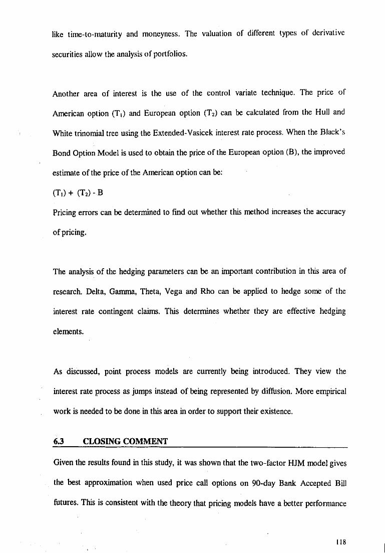
like time-to-maturity and moncyncss. The valuation of different types of derivative

securities allow the analysis of portfolios.

Another area of interest is the usc of the control variate technique. The price of

American option (T1) and European option (T2) can be calculated from the Hull and

White trinomial tree using the Extended-Vasicek interest rate process. When the Black's

Bond Option Model is used to obtain the price of the European option (B), the improved

estimate of the price of the American option can be:

(T,) + (T,)- B

Pricing errors can be determined to fmd out whether this method increases the accuracy

of pricing.

The analysis of the hedging parameters can be an important contribution in this area of

research. Delta, Gamma, Theta, Vega and Rho can be applied to hedge some of the

interest rate contingent claims. This detertnines whether they are effective hedging

elements.

As discussed, point process models are currently being introduced. They view the

interest rate process as jumps instead of being represented by diffusion. More empirical

work is needed to be done in this area in order to support their existence.

6.3 CLOSING COMMENT

Given the results found in this study, it was shown that the two-factor HJM model gives

the best approximation when used price call options on 90-day Bank Accepted Bill

futures. This is consistent with the theory that pricing models have a better performance

118

when the term structure of both the short-term and long-term rates arc included. The

results documented motivate cmpiric<.\1 studies of term structure models, where the

volatility is allowed to vary across the maturity of forward rates, as well a'i across time.

Challenging econometric problems are waiting along tWs route.

119

APPENDICES

I

I

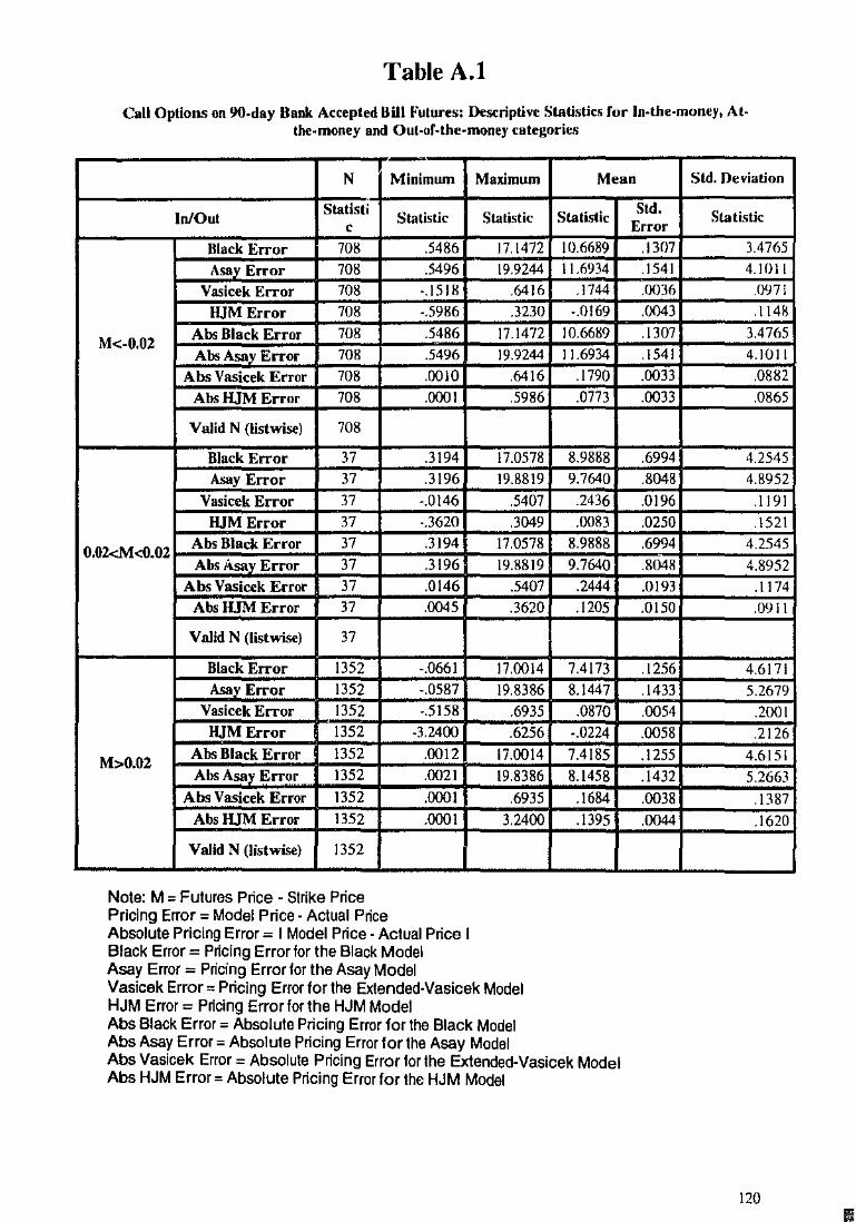
Table A.l

Call Options on 90-day Bank Accepted Dilll'utures: Descriptive Statistics for In-the-money, At· the-money and Out-of-the-money categories

-N Minimum Maximum Mean

In/Out Statisti

c

Black Error 708 Asay Error 708

Vasicek Error 708

IUM Error 708

M<-0.02 Abs Black Error 708 Abs Asay Error 708

Abs Vasicek Error 708 Abs HJM Error 708

Valid N (listwise) 708

Black Error 37 Asay Error 37

Vasicek Error 37

HJM Error 37

0.02<M<0.02 Abs Black Error 37 Abs Asay Error 37

Abs Vasicek Ecror 37 Abs lUM Error 37

V a1id N (list wise) 37

Black Error 1352 Asay Error 1352

Vasicek Error 1352 HJM Error 1352

M>0.02 Abs Black Error 1352 Abs A~y Error 1352

Abs Vasicek Error 1352 Abs HJM Error 1352

VaJid N (listwise) 1352

Note: M =Futures Price ·Strike Price Pricing Error= Model Price- Actual Price

Statistic

.5486

.5496 ·.1518 ·.5986 .5486 .5496 .0010 .000 I

.3194

.3196 ·.0146 ·.3620 .3194 .3196 .0146 .0045

-.0661 -.0587 -.5158

-3.2400 .0012 .0021

.0001

.0001

Absolute Pricing Error= I Model Price- Actual Price I Black Error= Pricing Error for the Black Model Asay Error= Pricing Error for the Asay Model

Statistic

17.1472 19.9244

.6416

.3230 17.1472 19.9244

.6416

.5986

17.0578 19.8819

.5407

.3049 17.0578 19.8819

.5407

.3620

17.0014 19.8386

.6935

.6256 17.0014 19.8386

.6935 3.2400

Vasicek Error= Pricing Error for the Extended-Vasicek Model HJM Error= Pncing Error for the HJM Model Abs Black Error= Absolute Pricing Error for the Black Model Abs Asay Error= Absolute Pricing Error for the Asay Model

Stalistic

10.6689 11.6934

.1744 -.0169

10.6689 11.6934

.1790

.0773

8.9888 9.7640 .2436 .0083

8.9888 9.7640

.2444

.1205

7.4173 8.1447 .0870

-.0224 7.4185 8.1458 .1684 .1395

Abs Vasicek Error= Absolute Pricing Error for the Extended-Vasicek Model Abs HJM Error= Absolute Pncing Error for tho HJM Model

Std. Error

.1307

.1541 JXJ36

.0043

.1307

.1541

.0033

.0033

.6994

.8048

.0196

.0250

.6994

.8048

.0193

.0150

.1256

.1433

.0054

.0058

.1255

.1432

.0038

.0044

Std. Deviation

Statistic

3.4765

4.1011 .(}971

.1148 3.4765 4.1011 .0882 .0865

4.2545 4.8952

.1191

.1521 4.2545 4.8952

.1174

.0911

4.6171 5.2679

.2001

.2126 4.6151 5.2663 .1387 .1620

120

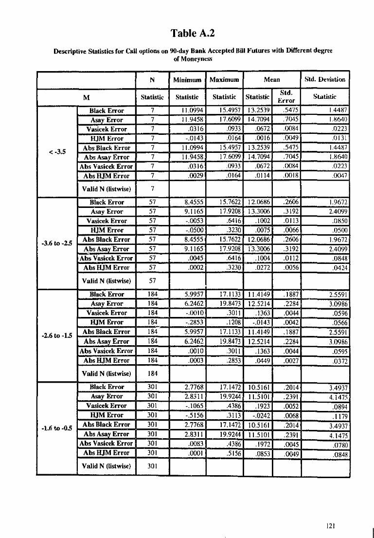
Table A.2

Descriptive Statistics for Call option.,. on 90-day Bank Accepted BUI Futures with Different degree of Moneynes.'i

N Minimwn Maximum Mean Std. Deviation

M Statistic Statistic Slatistic Statlstic Std.

Swti.~tic Error

Black Error 7 11.0994 15.4957 13.2539 .5475 1.4487

Asav Error 7 11.9458 17.6099 14.7094 .7045 I.H640

Vasicek Error 7 .0316 .0933 .0672 .(){)84 .0223

HJM Error 7 -.0143 .0164 .0016 .0049 .0131

< -3.5 Abs Black Error 7 11.0994 15.4957 I 3.2539 .5475 1.4487

Abs Asay Error 7 11.9458 17.6099 14.7094 .7045 1.8640

Abs Vasicek Error 7 .0316 .0933 .0672 .0084 .0223

Abs HJM Error 7 .0029 .0164 .0114 .0018 .0041

Valid N (listwise) 7

Black Error 57 8.4555 15.7622 12.0686 .2606 1.9672

Asay Error 57 9.1165 17.9208 13.3006 .3192 2.4099

Vasicek Error 57 -.0053 .6416 .I 002 .0113 .0850

HJM Error 57 -.0500 .3230 .0075 .0066 .0500

-3.6 to -2.5 Abs Black Error 57 8.4555 15.7622 12.0686 .2606 1.9672

Abs Asay Error 57 9.1165 17.9208 13.3006 .3192 2.4099

Abs Vasicek Error 57 .0045 .6416 .1004 .0112 .0848

Abs HJM Error 57 .0002 .3230 .0272 .0056 .0424

Valid N (listwise) 57

Black Error 184 5.9957 17.1133 11.4149 .1887 2.559! Asay Error 184 6.2462 19.8473 12.5214 .2284 3.0986

Vasicek Error 184 -.0010 .3011 .1363 .0044 .0596 HJM Error 184 -.2853 .1208 -.0143 .0042 .0566 -

-2.6 to -1.5 Abs Black Error 184 5.9957 17.1133 11.4149 .1887 2.5591

Abs Asay Error 184 6.2462 19.8473 12.5214 .2284 3.0986 Abs Vasicek Error 184 .0010 .3011 .1363 .0044 .0595

Abs HJM Error 184 .0003 .2853 .0449 .0027 .0372

Valid N (Ustwise) 184

Black Error 301 2.7768 17.1472 10.5161 .2014 3.4937 Asay Error 301 2.8311 19.9244 11.5101 .2391 4.1475

Vasicek Error 301 -.1065 .4386 .1923 .0052 .0894 IUMError 301 -.5156 .3113 -.0242 .0068 .1179

-U to -0.5 Abs Black Error 301 2.7768 17.1472 10.5161 .2014 3.4937 Abs Asay Error 301 2.8311 19.9244 11.5101 .2391 4.1475

Abs Vasicek Error 301 .0083 .4386 .1972 .0045 .0780 Abs HJM Error 301 .0001 .5156 .0853 .0049 .0848

Valid N (listwist) 301

121

Table A.2 (Cont'd)

N Minimum Maximum Mean Std. l)eviation

M Statistic Statistic Statistic Statistic Std.

Statistic Error

~Error ~I 75 17.12 H.996~ .1636 ""As;;y Error 751 19.9198 .IH90 5.1797

75 ·.3961 .668: 18" .1)()57 .1574

I HJM E;;::or 751 ·.854( .4881 ·.0149 .0069 .1888

-0.6 to 1.5 75 ~I 17.12 8.996~ .!636 Hffi ~Error 751 19.9198 .1890

lAb~ Error 75 £?I .668: .2153 .0043 16"

Abs HJM Error 751 .0001 .8540 .1356 .0048 .1321

Valid N (listwise) 751

~:;;:; 36(

~ 16.6153 ~ .2363

360 19.5191 .2725 5.1700 J7

16( -.433~ .693~ . )7~ .0104 .1974 R I Error 16( -.5680 .581 -.0128 .0104 riill 1.6 to 2.5 Abs Black Error 360 .0056 16.6153 s:t5T1 --:2362

Abs Asav Error 360 .0046 19.5191 8.9928 .2725 lAbs 'Error 360 .000 .6935 1564 .00 .1430

Abs 1JiE Error 360 .0003 .581 .1430 .0072 .1364

Valid N (listwise) 360

Black Error 260 -.032~ 6.0009 ~ Asav Error 260 -.0300 t8Tot 6.5864 4~ 260 -.4984 .69; .0050 .01 HJM Error !60 -3.2400 .6256 -.0311 .0175 .2819

2.6 to 3.5 Abs Black Error .0019 15.§ 6.()( .2492 I Abs Asay Error !60 .0040 1~3 6.5877 2s27 ~ 260

184 .I 326 .0091

26( .J09 .1486 .0150 .2414

Valid N (listwise) 260

I ~:;;:; 152 -.0574 10.7947 ]"}ill 2ill 152 4. .2606

k Error 152 -.5158 .371 -. .0140 .1725

Abs~;::or 152

~ .3799 -.( .0141 .1734

3.6 to 4.S !52 3ilil .2347 y Error 152 --4:0589 .2601 3.2064

lAbs 'Error !52 .00 .5158

·~ .0108 .1334

Abs~ 152 .0011 . .5078 .DIOS .1335

Valid N (listwise) !52

122

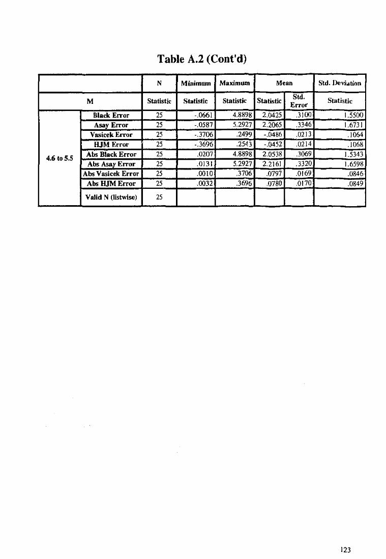
Table A.2 (Cont'd)

N Minimwn Maximum Mean Std. Deviation

M Statistic Statistic Statistic Statistic Std. Statistic Error

Black Error 25 -.0661 4.8898 2.0425 .3!00 1.551XJ

Asay Error 25 -.0587 5.2927 2.2065 .3346 1.673 I

Vasicek Error 25 -.3706 .2499 -.0486 .0213 .1064 HJM Error 25 -.3696 .2543 -.0452 .0214 .1068

4.6 toS.S Abs Black Error 25 .0207 4.8898 2.0538 .3069 1.5343 Abs Asay Error 25 .0131 5.2927 2.2!61 .3320 1.6598

Abs Vasicek Error 25 .0010 .3706 .0797 .0169 .0846

Abs RJM Error 25 .0032 .3696 .0780 .0!70 .0849

Valid N (listwise) 25

123

Table A.3

Descriptive Statistics for call options on 90-Day Bank Accepted Bill Futures with different time to maturily (days)

N Minimum Maximum Mean Std. Deviation

Time to Maturity (Days) Statistic Statistic Statistic Statistic Std. Statistic

Error Black Error 17 -.0425 .3194 .0365 JJ249 .1026

A~y Error 17 -.0400 .3196 .0378 .0247 .1020

Vasicek Error 17 -.0288 .0562 .()()()6 JXJ47 .0194

HJM Error 17 -.0287 .0390 -.0005 .0040 .fJJ 64

3 Abs Black Error 17 .0012 .3194 .0634 .()212 .0876

Abs Asay Error 17 .0021 .3196 .0626 .0214 .0881

Abs Vasicek Error 17 .0012 .0562 .0137 .0032 .0133

Abs HJM Error 17 .0013 .0390 .0125 .0024 .0101

Valid N (listwise) 17

Black Error 60 -.0661 1.3664 .2232 .0406 .3142

Asay Error 60 -.0587 J.l685 .2273 .0404 .3128

Vasicek Error 60 ·.0892 .1008 -.0183 .0048 .0369 -·-HJM Error 60 -.0890 .0750 -.0220 .0041 .0316

9 Abs Black Error 60 .0019 1.3664 .2430 .0386 .2989 Abs Asay Error 60 .0026 1.3685 .2435 .0387 .3002

Abs Vasicek Error 60 .0018 .1008 .0321 .0033 .0255

Abs HJM Error 60 .0020 .0890 .0294 .0032 .0248

Valid N (listwisc) 60

Black Error 18 .1159 1.6974 .6584 .1055 .4475 Asay Error 18 .1413 I. 7077 .6743 .1043 .4425

Vasicek Error 18 -.1121 .1105 -.0548 .0163 .0694 lUM Error 18 -.1114 .0359 -.0701 .0100 .0422

30 Abs Black Error 18 .1159 1.6974 .6584 .1055 .4475 Abs Asay Error 18 .1413 1.7077 .6743 .1043 .4425

Abs Vasicek Error 18 .0219 .1121 .0831 .0062 .0261 Abs HJM Error 18 .0294 .1114 .0775 .0059 .0251

Valid N (Ustwise) 18

Black Error 41 .0754 2.1416 .9824 .0936 .5996 Asay Error 41 .1075 2.1561 1.0038 .0930 .5953

Vasicek Error 41 -.3706 .1417 -.1248 .0277 .1771 lUM Error 41 -.3696 .0290 -.1466 .0262 .1675

37 Abs Black Error 41 .0754 2.1416 .9824 .0936 .5996 Abs Asay Error 41 .1075 2.1561 1.0038 .0930 .5953

Abs Vasicek Error 41 .0034 .3706 .1560 .0234 .1497 Abs HJM Error 41 .0025 .3696 .1554 .0248 .1591

Valid N (listwise) 41

124

Table A.3 (Cont'd)

N Minimwn Maximum Mean Std. l>cviation

Time to Maturity (Days) Stati.o>lic Statistic Statistic Statistic Sid. Statistic

Error

Black Error 17 -.0193 1.0882 .4269 ,[)<)33 .3!S47

Asay Error 17 .0200 1.09KO .4502 .IJ'!l 0 .3752

Vasicek Error 17 -.0830 .2321 -.0018 .0228 .fJ942

HJM Error 17 -.OKlO .1294 -.0252 .Oll9 .0572

44 Abs Black Error 17 .0091 1.0882 .4292 .IJ926 .3820

Abs Asay Error 17 .0200 1.0980 .4502 .ll910 .3752

Abs Vasicek Error 17 .0109 .2321 .0716 .0142 .0586

Abs IUM Error 17 .0096 .1294 .054( .0070 .0290

Valid N (listwise) 17

Black Error 40 .3711 3.9662 1.9653 .1582 1.0005

Asa_y Error 40 .4326 4.0297 2.0182 .1585 1.0023

Vasicek Error 40 -.0348 .2945 .1218 .0146 .0923

HJMError 40 -.0329 .1746 .0886 .0116 .0735

72 Abs Black Error 40 .3711 3.9662 1.9653 .1582 1.0005

Abs Asay Error 40 .4326 4.0297 2.0182 .1585 1.0023

Abs Vasicek Error 40 .0001 .2945 .1283 .0131 .0828

Abs HJM Error 40 .0015 .1746 .0950 .0103 .0649

Valid N (listwise) 40

Black Error 24 .8104 2.7901 1.8206 .1364 .6683 A.say Error 24 .8895 2.8274 1.8759 .1337 .6548

Vasicek Error 24 -.0897 .1838 -.0006 .0176 .0863

IUMError 24 -.0880 .0589 -.0270 .0086 .0423

79 Abs Black Error 24 .8104 2.7901 1.8206 .1364 .6683 Abs Asay Error 24 .8895 2.8274 1.8759 .I 337 .6548

Abs Vasicek Error .24 .0014 .1838 .0687 .0103 .0503

Abs lUM Error 24 .0079 .0880 .0445 .0045 .0222

Valid N (listwise) 24

Black Error 20 1.0762 3.5110 2.0532 .1580 .7068 Asay Error 20 1.1827 3.5882 2.1298 .1554 .6950

Vasicek Error 20 -.0332 .3020 .0739 .0252 .1127 IUMError 20 -.0315 .2050 .0437 .0166 .0744

93 Abs Black Error 20 1.0762 3.5110 2.0532 .1580 .7068 Abs Asay Error 20 1.1827 3.5882 2.1298 .1554 .6950

Abs Vasicek Error 20 .0016 .3020 .0852 .0233 .1040 Abs HJM Error 20 .0015 .2050 .0539 .0150 .0670

Valid N (listwise) 20

125

Table A.3 (Cont'd)

N Minimwn Maximum Mean Std. I>eviation

Statistic Time to Maturity (Days) Statistic Statistic Statl'itic Statistic :r~~r

~~; :=;;:;-+-·-:: :8~33+--: :~.·~2~~~:517:+--~ :4.':"';65 55d-4c....,~~~~~~~.:;:~ ;;~:s78sl---.d~~~4- 1

100

<Error 83 (01 .39 .089f .0(]( .1181

~~H~~I~Erro~·r-~883~~--~009r-~~-2903~~~51~C~.rn~~9r---~·®I~IO: -~bs •~ack Error 83 I 169( 4.55 ~ .088 .8041 A~rror 83 1.2757 4.654c 2.786( .0878 .7997

I Abs~ Error 83 .003 .3923 .113( . 'J I 0 .0957 Abs HJM Error 83 .0001 .2903 .0777 .0075 .068

Valid N (listwise) 83

t---;~~ :~f.~~· ;~ ~8 4

;;; ~ill: m: m; IZ1

128

Abs Black Error 19 1.9398 4.728! H§k .182 .794 Abs~AsayError 19 2.1058 .1~ .7759

I Abs ;:;::,:' E=rro::...t-'-...;.;;-19-1_,.;;·01~24+--;;·222~39f--.'~15~44-..::. :0:,.!.::::;::.!..---'-~05:.:;.!59 Abs !Error 19 .011 .2204 .1325 .0172 .0749

Valid N (listwise) 19

Black Error 45 1.4936 4.3198 2.9 .1164 . 7809

'iijM ror 45 .0285 -- J' .0298 -;~ A~ '=.=•ro•-r-~44:5~;--1~1.4~936+--~41 .. 7,337~98-~22 .. 9~~05-~~-----'-~'"~® AbsAsay error 45 1.6364 4.4945 3~ .114 \79

fiA~bs~~~<~Errttor:3t45:t==-~-COO£tt28===.4~47~38~ ~+-...;·~025+---~-1~690 1- AliSHJMError 45 .0004 .0292 .1958

Valid N (listwise)

r---+1-;;;:::;:--'Error

~Error

45

19 1.933 H~2 3.1675 .2229 .9714 19 2.0006 5,;;::!22 3.2991 .2232 .9730

135

I A!'bs~E::-t--7,;-19-i---':.00~2:f-~-2~9no-;::.J--'·~ 1449:.1---*' .. o JI~ 9o ___ _;.0~8l:2g.j9 = 19 .0142 .1532 .104: .0089 .0386

Valid N (listwise) 19

126 I

Table A.3 (Cont'd)

N Minimwn Maximum Mean Std. Deviation

Time to Maturity (Days) Statistic Statbtic Statistic Statistic Std.

Statistic Error

Black Error 22 4.896\ 6.5213 5.H596 .\021 .4791

Asay Error 22 5.1386 6.7230 6.0646 .IJ9H4 .4615

Vasicek Error 22 .069\ .3322 .2016 .0195 .()9] 3

HJM Error 22 .0348 .1698 .1123 .0088 .1!412

142 Abs Black Error 22 4.896\ 6.5213 5.H596 .\021 .4791

Abs Asay Error 22 5.1386 6.7230 6.0646 .0984 .4615

Abs Vasicek Error 22 .069\ .3322 .2016 .0195 .0913

Abs HJM Error 22 .0348 .\698 .1123 .0088 .1!412

Valid N (listwise) 22

Black Error 43 3.3258 6.4872 4.8105 .\309 .8584

Asay Error 43 3.5468 6.7242 5.0122 .\304 .8551

Vasicek Error 43 .0192 .3778 .2376 .0159 .1041

HJM Error 43 .0056 .2945 .1649 .0158 .\037

163 Abs Black Error 43 3.3258 6.4872 4.8\05 .\309 .8584

Abs Asay Error 43 3.5468 6.7242 5.0122 .JJ04 .8551

Abs Vasicek Error 43 .0192 .3778 .2376 .0159 .1041

Abs HJM Error 43 .0056 .2945 .\649 .0\58 .\037

Valid N (listwise) 43

Black Error 26 3.0266 5.6335 4.3850 .1555 .7927

Asay Error 26 3.2505 5.8181 4.5637 .1508 .7690 Vasicek Error 26 ·.0631 .2398 .0542 .:1209 .1064

IUM Error 26 ·.0584 .0739 ·.0010 .0075 .0382

170 Abs Black Error 26 3.0266 5.6335 4.3850 .1555 .7927 Abs Asay Error 26 3.2505 5.8181 4.5637 .1508 .7690

Abs Vasicek Error 26 .0005 .2398 .0878 .0156 .0798

Abs HJM Error 26 .0035 .0739 .0319 .0039 .0\99

Valid N (listwise) 26

Black Error 39 3.7224 7.0662 5.7300 .1609 1.0047 Asay Error 39 3.9953 7.3523 5.9870 .1633 1.0\96

Vasicek Error 39 .0096 .3738 .1937 .0176 .\097 lUM Error 39 .0099 .2871 .0933 .0110 .0685

184 Abs Black Error 39 3.7224 7.0662 5.7300 .1609 1.0047 Abs Asay Error 39 3.9953 7.3523 5.9870 .1633 1.0196

Abs Vasicek Error 39 .0096 .3738 '1937 .0176 .1097 Abs HJM Error 39 .0099 .2871 .0933 .0110 .06S5

Valid N (listwise) 39

127

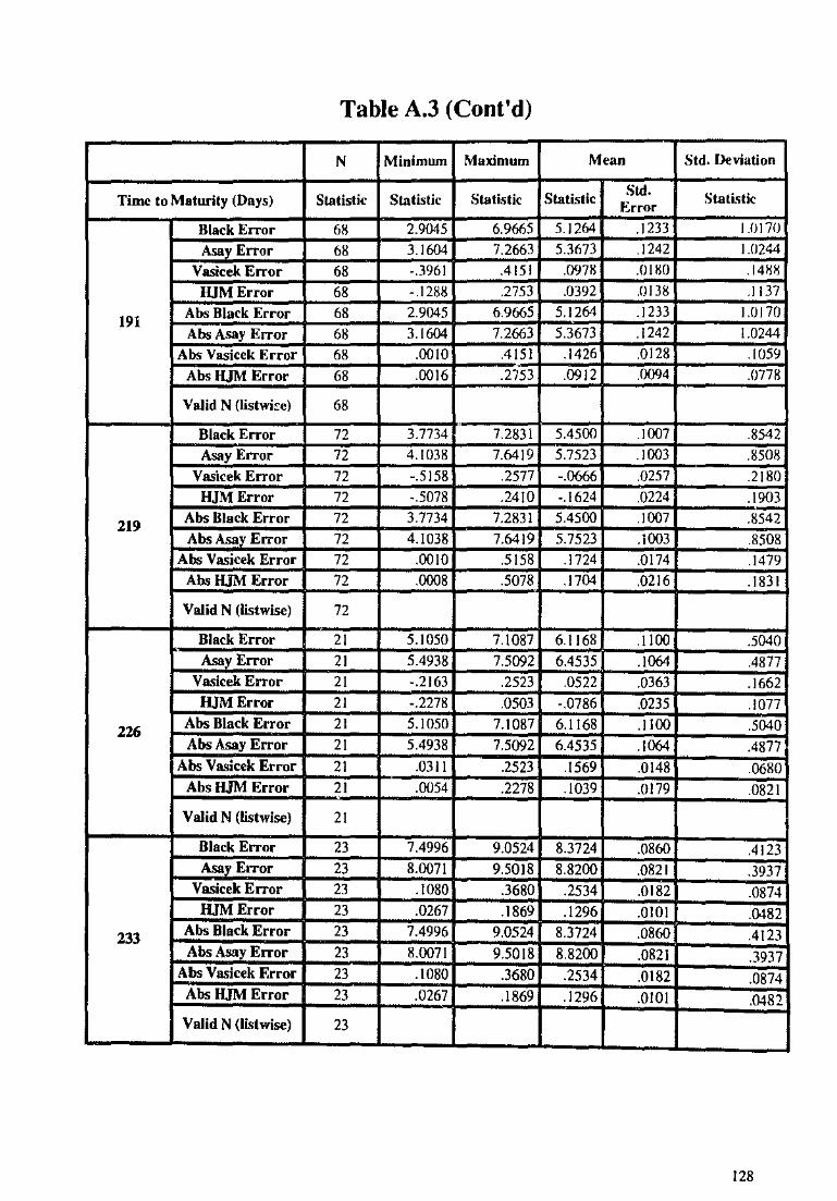
Table A.3 (Cont'd)

N Minimum Maximum Mean Std. I>eviation

Time to Maturity (Days) Statistic Statistic Statistic Statio;tic Std. Statistic

Error

Black Error 68 2.9045 6.9665 5.1264 .1233 I .0170

Asay Error 68 3.1604 7.2663 5.3673 .1242 I.(J244

Vasicek Error 68 -.3961 .4151 .0978 .OIIW .14HH

HJM Error 68 -.1288 .2753 .0392 JJI 38 .1137

191 Abs Black Error 68 2.9045 6.9665 5.1264 .1233 1.0170

Abs Asay Error 68 3.1604 7.2663 5.3673 .1242 1.0244

Abs Vasicek Error 68 .0010 .4151 .1426 .0128 .1059

Abs lUM Error 68 .0016 .2753 .0912 .0094 .0778

Valid N {listwi~e) 68

Black Error 72 3.7734 7.2831 5.4500 .1007 .8542

Asay Error 72 4.1038 7.6419 5.7523 .1003 .8508

Vasicek Error 72 -.5158 .2577 -.0666 .0257 .2180

HJM Error 72 -.5078 .2410 -.1624 .0224 .1903

219 Abs Black Error 72 3.7734 7.2831 5.4500 .1007 .8542

Abs Asay Error 72 4.1038 7.6419 5.7523 .1003 .8508 Abs Vasicek Error 72 .0010 .5158 .1724 .0174 .1479

Abs HJM Error 72 .0008 .5078 .1704 .0216 .1831

Valid N (listwise) 72

Black Error 21 5.1050 7.1087 6.1168 .1100 .5040 Asay Error 21 5.4938 7.5092 6.4535 .1064 .4877

Vasicek Error 21 -.2163 .2523 .0522 .0363 .1662 IUM Error 21 -.2278 .0503 -.0786 .0235 .1077

226 Abs Black Error 21 5.1050 7.1087 6.1168 .1100 .5040 Abs Asay Error 21 5.4938 7.5092 6.4535 .1064 .4877

Abs Vasicek Error 21 .0311 .2523 .1569 .0148 .0680 Abs HJM Error 21 .0054 .2278 .1039 .0179 .0821

Valid N (listwise) 21

Black Error 23 7.4996 9.0524 8.3724 .0860 .4123 Asay Error 23 8.0071 9.5018 8.8200 .0821 .3937

Vasicek Error 23 .1080 .3680 .2534 .0182 .0874 HJM Error 23 .0267 .1869 .1296 .0101 .0482

233 Abs Black Error 23 7.4996 9.0524 8.3724 .0860 .4123 Abs Asa_y Error 23 8.0071 9.5018 8.8200 .0821 .3937

Abs Vasicek F.rror 23 .1080 .3680 .2534 .0182 .0874 Abs HJM Error 23 .0267 .1869 .1296 .0101 .0482

Valid N (listwise) 23

128

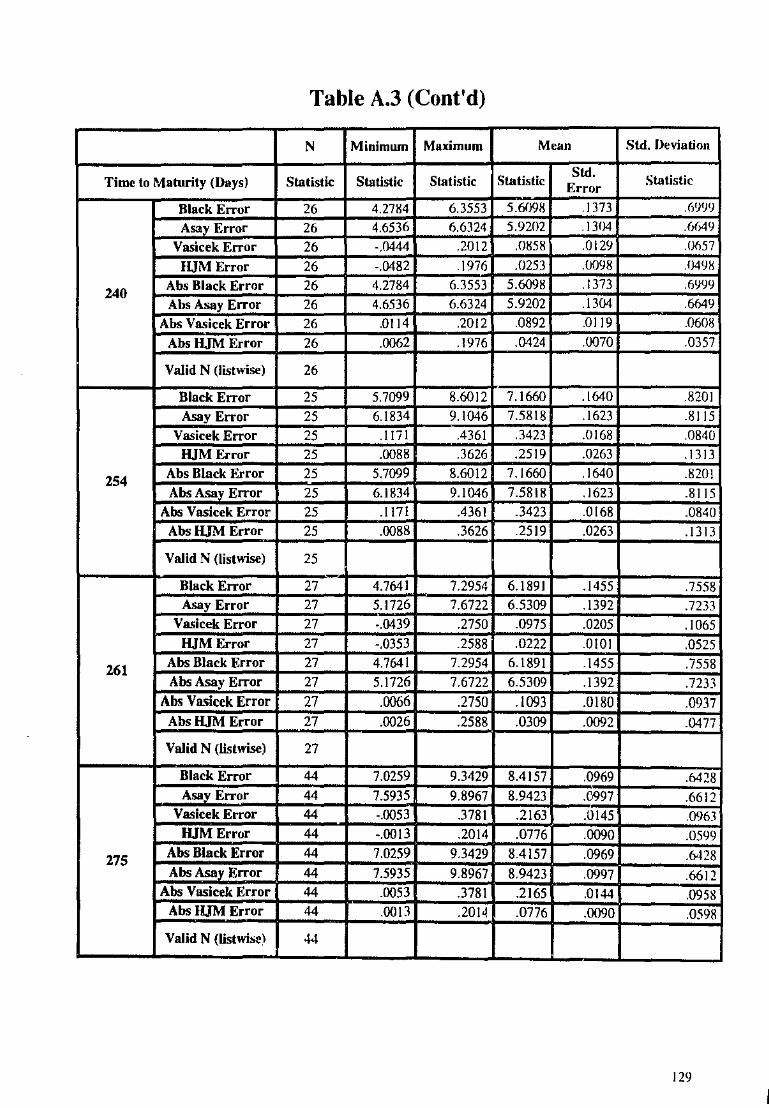
Table A.3 (Cont'd)

N Minimum Maximum Mean Std. Deviation

Time to Maturity (Days) Statistic Statistic Statistic Statistic Std.

Statistic Error

Black Error 26 4.2784 6.3553 5.611!8 .1373 ,(ii)IJ!)

Asay Error 26 4.6536 6.6324 5.9202 .1304 .6649

Vasicek Error 26 -.0444 .2012 .0858 .0129 .0()57

HJM Error 26 -.0482 .1976 .0253 .0098 .f)49!S

240 Abs Black Error 26 4.2784 6.3553 5.6098 .1373 .6999

Abs Asay Error 26 4.6536 6.6324 5.9202 .1304 .6649

Abs Vasicek Error 26 .0114 .2012 .0892 .0119 .0608

Abs lUM Error 26 .0062 .1976 .0424 .0070 .0357

Valid N (listwise) 26

Black Error 25 5.7099 8.6012 7.1660 .1640 .8201 Asay Error 25 6.1834 9.1046 7.5818 .1623 .8115

Vasicek Error 25 .1171 .4361 .3423 .0168 .0840 HJM Error 25 .0088 .3626 .2519 .0263 .1313

254 Abs Black Error 25 5.7099 8.6012 7.1660 .1640 .8201 Abs Asav Error 25 6.1834 9.1046 7.5818 .1623 .8115

Abs Vasicek Error 25 .1171 .4361 .3423 .0168 .0840 Abs IUM Error 25 .0088 .3626 .2519 .0263 .1313

Valid N (listwise) 25

-Black Error 27 4.7641 7.2954 6.1891 .1455 .7558 Asay Error 27 5.1726 7.6722 6.5309 .1392 .7233

Vasicek Error 27 -.0439 .2750 .0975 .0205 .1065 HJM Error 27 -.0353 .2588 .0222 .0101 .0525

261 Abs Black Error 27 4.7641 7.2954 6.1891 .1455 .7558 Abs Asay Error 27 5.1726 7.6722 6.5309 .1392 .723)

Abs Vasicek Error 27 .0066 .2750 .1093 .0180 .0937 Abs HJM Error 27 .0026 .2588 .0309 .0092 .0477

Volid N (listwise) 27

Black Error 44 7.0259 9.3429 8.4157 .0969 .6428 Asay Error 44 7.5935 9.8967 8.9423 .C997 .6612

Vasicek Error 44 -.0053 .3781 .2163 .0145 .0963 HJM Error 44 -.0013 .2014 .0776 .0090 .0599

275 Abs Black Error 44 7.0259 9.3429 8.4157 .0969 .6428 Abs Asay Error 44 7.5935 9.8967 8.9423 .0997 .6612

Abs Vasicek Error 44 .0053 .3781 .2165 .0144 .0958 Abs IUM Error 44 .0013 .201< .0776 .0090 .0598

Valid N (listwist\ -l4

129

ll

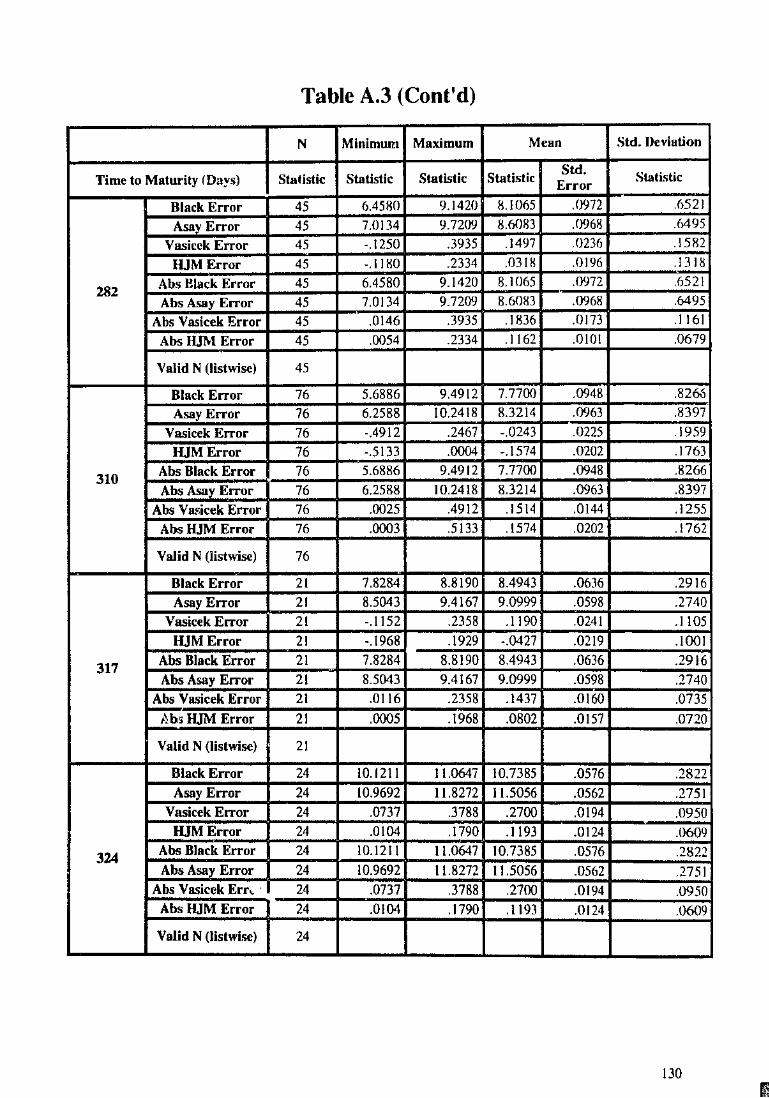
Table A.3 (Cont'd)

N Minimwn Maximum Mean Std. Deviation

Time to Maturity rDays) Statistic Statistic Statistic Statistic Std.

Statistic Error

Black Error 45 6.45HO 9.1420 8.1065 .(J972 .6521

Asay Error 45 7.0134 9.720'! 8.60H3 .0968 .6495

Vasicek Error 45 -.1250 .3935 .1497 .0236 .15H2

HJM Error 45 -.1180 .2334 .0318 .() 196 .1318

282 Abs Black Error 45 6.4580 9.1420 8.1065 .0972 .6521

Abs Asay Error 45 7.0134 9.720'! 8.6083 .0968 .6495

Abs Vasicek Error 45 .0146 .3935 .1836 .0173 .1161

Abs HJM Error 45 .0054 .2334 .1162 .0101 .0679

Valid N (listwise) 45

Black Error 76 5.6886 9.4912 7.7700 .0948 .82&1

Asay Error 76 6.2588 10.2418 8.3214 .0963 .8397

Vasicek Error 76 -.4912 .2467 -.0243 .0225 .1959

HJM Error 76 -.5133 .0004 -.1574 .0202 .1763

310 Abs Black Error 76 5.6886 9.4912 7.7700 .0948 .8266

Abs Asay Error 76 6.2588 10.2418 8.3214 .0963 .8397 Abs Vm:icek Error 76 .0025 .4912 .1514 .0144 .1255

Abs IUM Error 76 .0003 .5133 .1574 .0202 .1762

Valid N (listwise) 76

Black Error 21 7.8284 8.8190 8.4943 .0636 .2916 Asay Error 21 8.5043 9.4167 9.0999 .0598 .2740

Vasicek Error 21 -.1152 .2358 .1190 .0241 .1105 HJM Error 21 -.1968 .1929 -.0427 .0219 .1001

317 Abs Black Error 21 7.8284 8.8190 8.4943 .0636 .2916 Abs Asay Error 21 8.5043 9.4167 9.0999 .0598 .2740

Abs Vasicek Error 21 .0116 .2358 .1437 .0160 .0735 .. ~b~ HJM Error 21 .0005 .1968 .0802 .0157 .0720

Valid N (listwise) 21

Black Error 24 10.1211 11.0647 10.7385 .0576 .2822

Asay Error 24 10.9692 11.8272 11.5056 .0562 .2751 Vasicek Error 24 .0737 .3788 .2700 .0194 .0950

HJM Error 24 .0104 .1790 .1193 .0124 .0609

324 Abs Black Error 24 10.1211 11.0647 10.7385 .0576 .2822 Abs Asay Error 24 10.9692 11.8272 11.5056 .0562 .2751

Abs Vasicek Err.._ · 24 .0737 .3788 .2700 .0194 .0950 Abs fUM Error 24 .0104 .1790 .1193 .0124 .tJ609

Valid N (listwise) 24

130

Table A.3 (Cont'd)

N Minimum Maximum Mean Std. Deviation

Time to Maturity (Days) Statistic Statistic Statistic Statistic Std. Statistic

Error

Black Error 25 5.9232 7.9676 7.2544 .1370 /iHSO

Asay Error 25 6.5302 8.4468 7.7797 .127() .6394

Vasicek Error 25 .00 II .1846 .(!947 .0124 .06!9

HJM Error 25 ·.0992 .0431 -.0()1}3 .0102 .0512

331 Abs Black Error 25 5.9232 7.9676 7.2544 .1370 .6850

Abs Asay Error 25 6.5302 8.4468 7. 7797 .1279 .6394

Abs Vasicek Error 25 .0011 .1846 .0947 .0124 .0619

Abs HJM Error 25 .0126 .0992 .0447 .0050 .0252

VaJid N (listwise) 25

Black Error 24 7.8324 9.6537 9.0233 .1186 .5809

Asay Error 24 8.6069 10.3063 9.7122 .1099 .5385

Vasicek Error 24 .1575 .4424 .3668 .0156 .0766 lUM Error 24 ·.0044 .3903 .2493 .0301 .1475

345 Abs Black Error 24 7.8324 9.6537 9.0233 .1186 .5809 Abs Asay Error 24 8.6069 10.3063 9.7122 .1099 .5385

Abs Vasicek Error 24 .1575 .4424 .3668 .01.'6 .0766 Abs HJM Error 24 .0044 .3903 .2497 .0300 .1469

Valid N (listwise) 24

Black Error 25 6.5076 8.5594 7.8493 .1374 .6871 Asay Error 25 7.1448 9.0727 8.4062 .1284 .6422

Vasicek Error 25 ·.0202 .2869 .(403 .0215 .1075 HJM Error 25 ·.0089 .0333 .0174 .0023 .0116

352 Abs Black Error 25 6.5076 8.5594 7.8493 .1374 .6871 Ab:; Asay Error 25 7.1448 9.0727 8.4062 .1284 .6422

Abs Vasicek Error 25 .0063 .2869 .1431 .0207 .1036 Abs HJM Error 25 .0011 .0333 .0181 .0021 .0104

Valid N (listwisc) 25

Black Error 46 9.3674 I \.8417 10.7518 .1207 .8188 Asay Error 46 10.0799 12.7788 I \.6240 .1302 .8829

Vasicek Error 46 .0316 .3755 .2109 .0140 .0948 IUM Error 46 -.0436 .1745 .0474 .0111 .0755

366 Abs Black Error 46 9.3674 I \.8417 10.7518 .1207 .8188 Abs Asay Error 46 10.0799 12.7788 11.6240 .1302 .8829

Abs Vasicek Error 46 .0316 .3755 .2109 .0140 .0948 Abs HJM Error 46 .0046 .1745 .0652 .0089 .0604

Valid N (listwise) 46

131

Table A.3 (Cont'd)

N Maximum Mean Std. DHiation

Time to Maturity (Days) Statistic Statistic Statistic Statistic :..~~r Statistic

Black Error 4 H.617C 1.1 .25( .1001 .6R95

A"'Y Error 47 11.071 .103' .7ll2

'Error 4' ~ .3799 .158~ .022' .153 I

H l Error 47 .2077 .0153 .()2(){ .I 369

373 . Abs !lack Error 41 1 .181 .2501 .1001 .6895

r Error 47 11.0711 .103' .7ll

[.Abs 4' .008 .3799 .186~

~ .l16:

Abs HJM Error 47 .016C .2077 .1241 .( .0569

Valid N (listwise) 47

Black Error 22 8.5888 .JOSS .4965 Asay Error 22 9.571( ll.l927 I . .0961'

~ ~~:;r 22 ·.15 .2108 .)644 .0257

22 ·.172 .0020 .J9S: 126 .0592

394 k Error 22 .1059 .496:

Abs~yError 9.5710

"4127 l0.5m .c 961 Jill lAbs k Error !39 . 108 .12 12:

Abs HJM Error .002C . 721 .0983 ,( 121 .0592

Valid N (listwise) 22

Black Error 49 7.69 9.25 .0906 .6343 ~y Error 49 8.5663 10.8138 .0872 .6101

· 'Error 49 .2178 .025: .1771 ""jjjM Error 49 .1974 ·.195~

~: .1956

401 Abs Black Error 49 7.69 9.251 .6343 Abs Asay Error 49

~ Jill

.0872 .6101

LAbs k Error 49 Jill -Fz7;~ .1159

Abs HJM Error 49 ~ .2036 .1870

Valid N (listwise) 49

'"'iii,;cl;' Error 24 9.4132 11.1407

.~ .4666

~Y Error 24 12. 11.646: .5025 24 .2474 .01781 ]ill HJM Error 24 1709 .0159 .012'

408 Abs Black Error 24 9. 4132 II. 1407

~ .4666

~:;.:r 12.1172 11.646: .5025

.0056 .2474

~ .0144 )7(

.. Abs HJM Error .0002 .1709 .0121 .0592

Valid N (l~stwise) 24

132 I

Table A.3 (Cont'd)

N Minimum Maximum Mean Std. Ueviation

Time to Maturity (Days) Statistic Statistic Statistic Statistic Std. Statlo;tic

Error Black Error 25 11.6919 13.62!XJ 13.1345 .1045 .5223

Asay Error 25 12.'1040 14.8403 14.3432 .1135 .5675 Vasicek Error 25 .1453 .6935 .5156 .0370 .1851

HJM Error 25 .0322 .6256 .3499 .0409 .2043

415 Abs Black Error 25 11.6919 13.tJ200 13.1345 .1045 .5223 Abs Asay Error 25 12.7040 14.8403 14.3432 .1135 .5675

Abs Vasicek Error 25 .1453 .6935 .5156 .0370 .1851 Abs HJM Error 25 .0322 .6256 .3499 .0409 .2043

Valid N (listwise) 25

Black Error 27 7.6912 9.5436 8.9625 .1120 .5817 Asay Error 27 8.5723 10.2782 9.7376 .1020 .5301

Vasicek Error 27 .0267 .1763 .1022 .0096 .0499 IUM Error 27 -.1418 .0614 -.0242 .0135 .0702

422 Abs Black Error 27 7.6912 9.5436 8.9625 .1120 .5817 Abs Asay Error 27 8.5723 10.2782 9.7376 .1020 .5301

Abs Vasicek Error 27 .0267 .1763 .1022 .0096 .0499 Abs HJM Error 27 .0036 .1418 .0618 .0076 .0397

Valid N (listwist) 27

Black Error 25 9.6172 I 1.3520 10.8235 .1106 .5531 . Asay Error 25 10.7370 12.3250 11.8394 .0999 .4993

Vasicek Error 25 .1254 .4198 .3411 .0176 .0879 HJM Error 25 -.6328 .3766 .1561 .0454 .2271

436 Abs Black Error 25 9.6172 I 1.3520 10.8235 .1106 .553 I Abs Asay Error 25 10.7370 12.3250 11.8394 .0999 .4993

Abs Vasicek Error 25 .1254 .4198 .3411 .0176 .0879 Abs HJM Error 25 .0005 .6328 .2133 .0344 .1720

Valid N (listwise) 25

Black Error 72 8.4218 11.1666 10.2928 .0795 .6742 Asay Error 72 9.3472 12.0327 11.1460 .0790 .6703

Vasicek Error 72 -.0186 .2816 .1638 .0096 .0816 HJM Error 72 -.1095 .1257 -.0308 .0046 .0388

450 Abs Black Error 72 8.4218 11.1666 10.2928 .0795 .6742 Abs Asay Error 72 9.3472 12.0327 11.1460 .0790 .6703

Abs Vasicek Error 72 .0023 .2816 .1644 .0095 .0804 Abs fUM Error 72 .0002 .1257 .0353 .0041 .0347

Valid N (listwise) 72

133

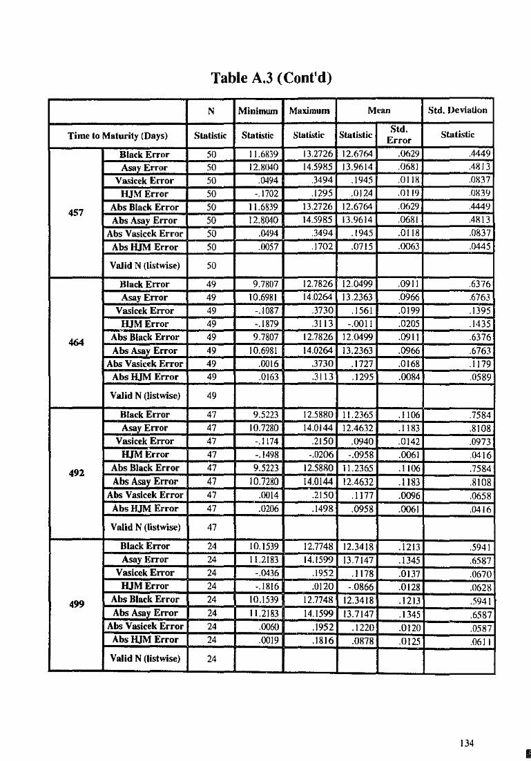
Table A.3 (Cont'd)

N Minimwn Maximum Mean Std. !leviation

Time to Maturity (Days) Statistic Statistic Statistic Statistic Std.

Statistic Error

Black Error 50 11.6839 13.2726 12.6764 .!!629 .4449

Asay Error 50 12.8040 14.5985 13.9614 .0681 .4813

Vasicek Error 50 .0494 .3494 .1945 .0118 .0837

HJM Error 50 ·.1702 .1295 .0124 .0119 .OH39

457 Abs Black Error 50 11.6839 13.2726 12.6764 .0629 .4449

Abs Asay Error 50 12.8040 14.5985 13.9614 .0681 .4813

Abs Vasicek Error 50 .0494 .3494 .1945 .0118 .0837

Abs IUM Error 50 .0057 .1702 .0715 .0063 .0445

Valid N {listwise) 50

Black Error 49 9.7807 12.7826 12.0499 .0911 .6376

Asay Error 49 10.6981 14.0264 13.2363 .0966 .6763

Vasicek Error 49 -.1087 .3730 .1561 .0199 .1395

HJM Error 49 -.1879 .3113 -.0011 .0205 .1435

464 Abs Black Error 49 9.7807 12.7826 12.0499 .0911 .6376

Abs Asav Error 49 10.6981 14.0264 13.2363 .0966 .6763

Abs Vasicek Error 49 .0016 .3730 .1727 .0168 .1179 Abs HJM Error 49 .0163 .3113 .1295 .0084 .0589

Valid N (listwise) 49

Black Error 47 9.5223 12.5880 11.2365 .1106 .7584 Asay Error 47 10.7280 14.0144 12.4632 .1183 .8108

Vasicek Error 47 -.1174 .2150 .0940 .0142 .0973 HJM Error 47 -.1498 -.0206 -.0958 .0061 .0416

492 Abs Black Error 47 9.5223 12.5880 11.2365 .1106 .7584 Abs Asay Error 47 10.7280 14.0144 12.4632 .1183 .8108

Abs Vasicek Error 47 .0014 .2150 .1177 .0096 .0658 Abs HJM Error 47 .0206 .1498 .0958 .0061 .0416

Valid N (listwise) 47

Black Error 24 10.1539 12.7748 12.3418 .1213 .5941 Asay Error 24 11.2183 14.1599 13.7147 .1345 .6587

Vasicek Error 24 -.0436 .1952 .1178 .0137 .0670 HJMError 24 -.1816 .0120 -.0866 .0128 .0628

499 Abs Black Error 24 10.1539 12.7748 12.3418 .1213 .5941 Abs Asay Error 24 11.2183 14.1599 13.7147 .1345 .6587

Abs Vasicek Error 24 .0060 .1952 .1220 .0120 .0587 Abs HJM Error 24 .0019 .1816 .0878 .0125 .0611

Valid N (listwise) 24

134

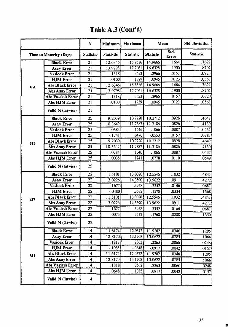
Table A.3 (Cont'd)

N Minimwn Maximum Mean Std. Deviation

Time to Maturity (Days) Statistic Statistic Statistic Statistic Std. Statistic

Error

Black Error 21 12.6346 15.8586 14.9666 .1664 .7627

Asav Error 21 13.9798 17.7061 16.6328 .1900 .8707

Vasicek Error 21 .1318 .3653 .2966 .0157 .0720

HJM Error 21 .0100 .1929 .0945 .0123 .0563

506 Abs Black Erro-r 21 12.6346 15.8586 14.9666 .1664 .7627

Abs Asay Error 21 13.9798 17.7(){;1 16.6328 .1900 .H707

Abs Vasicek Error 21 .1318 .3653 .2966 .0157 .0720

Abs HJM Error 21 .QIOO .1929 .0945 .0123 .0563

Valid N (listwise) 21

Black Error 25 9.2039 10.7220 10.2712 .0928 .4642 Asay Error 25 10.3649 11.7387 11.3186 .0826 .4130

Vasicek Error 25 .0384 .1646 .1066 .0087 .0437 HJM Error 25 -.1741 .0476 -.0553 .0157 .0783

513 Abs Black Error 25 9.2039 10.7220 10.2712 .0928 .4642 Abs Asay Error 25 10.3649 11.7387 11.3186 .0826 .4130

Abs Vasicek Error 25 .0384 .1646 .1066 .0087 .0437 Abs HJM Error 25 .0038 .1741 .0778 .OliO .0549

Valid N (listwise) 25

Black Error 22 11.5101 I 3.0020 12.5546 .1032 .4843 -Asay Error 22 13.0226 14.3590 13.9622 .0911 .4?72

Vasicek Error 22 .1677 .3958 .3352 .0146 .0687 HJM Error 22 -.0480 .3532 .1578 .0334 .1568

527 Abs Black Error 22 11.5101 13.0020 12.5546 .1032 .4843 Abs Asay Error 22 13.0226 14.3590 13.9622 .0911 .4272

Abs Vasicek Error 22 .1677 .3958 .3352 .0146 .0687 Abs HJM Error 22 .0073 .3532 .1760 .0288 .1350

Valid N (listwise) 22

Black Error 14 11.6174 12.0372 11.9202 .0346 .1295 Asay Error 14 12.8170 ll.1708 13.0622 .0285 .1066

Vasicek Error 14 .1818 .2562 .2263 .0066 .0248 HJM Error 14 -.1085 -.(){;48 -.0917 .0042 .0157

541 Abs Black Error 14 11.6174 12.0372 11.9202 .0346 .1295 Abs Asay Error 14 12.8170 13.1708 13.(){;22 .0285 .1066

Abs Vasicek Error 14 .1818 .2562 .2263 _Q(){i6 .0248 Abs HJM Error 14 .0648 .1085 .0917 .0042 .0157

Valid N (l~twise) 14

135

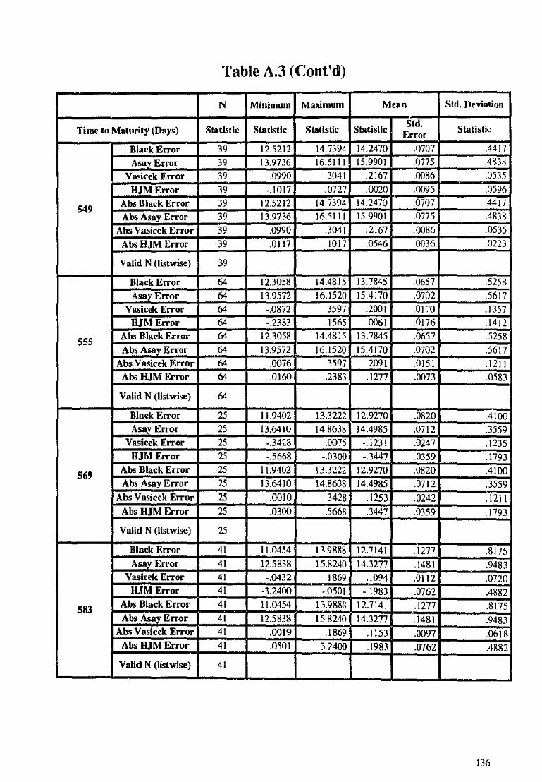
Table A.3 (Cont'd)

N Minimum Maximum Mean Std. Deviation

Time to Maturity (Days) Statistic Statistic Statistic Statistic Std.

Statistic Error

Black Error 39 12.5212 14.7394 14.2470 Jl707 .4417

ASIJ.r Error 39 13.9736 16.5111 15.9901 .0775 ,4g]g

Vasicek Error 39 .0990 .3041 .2167 .0086 .0535

HJM Error 39 ·.1017 .0727 .0020 .0095 .0596

549 Abs Black Error 39 12.5212 14.7394 14.2470 .0707 .4417

Abs Asay Error 39 I 3.9736 16.511 I 15.9901 .0775 .483g

Abs Vasicek Error 39 .0990 .3041 .2167 .0086 .0535

Abs HJM Error 39 .0117 .1017 .0546 .0036 .0223

Valid N (listwise) 39

Black Error 64 12.3058 14.4815 I 3. 7845 .0657 .5258

Asay Error 64 I 3.9572 16.1520 15.4170 .0702 .5617

Vasicek Error 64 -.0872 .3597 .2001 .0170 .I 357

HJM Error 64 -.2383 .1565 .0061 .0176 .1412

555 Abs Black Error 64 12.3058 14.4815 13.7845 .0657 .5258

Abs Asay Error 64 13.9572 16.1520 15.4170 .0702 .5617 Abs Vasicek Error 64 .0076 .3597 .2091 .0151 .1211

Abs IUM Error 64 .0160 .2383 .1277 .0073 .0583

Valid N (Ustwise) 64

Black Error 25 11.9402 13.3222 12.9270 .0820 .4100 Asay Error 25 13.6410 14.8638 14.4985 .0712 .3559

Vasicek Error 25 -.3428 .0075 ·.123 I .0247 .1235 HJM Error 25 ·.5668 -.0300 -.3447 .0359 .1793

569 Abs Black Error 25 11.9402 13.3222 12.9270 .0820 .4100 Abs Asay Error 25 13.6410 14.8638 14.4985 .0712 .3559

Abs Vasicek Error 25 .0010 .3428 .1253 .0242 .1211 Abs HJM Error 25 .0300 .5668 .3447 .0359 .1793

Valid N (listwlse) 25

Black Error 41 11.0454 13.9888 12.7141 .1277 .8175 Asay Error 41 12.5838 15.8240 14.3277 .1481 .9483

Vasicek Error 41 -.0432 .1869 .1094 .0112 .0720 HJM Error 41 -3.2400 -.050! -.1983 .0762 .4882

583 Abs Black Error 41 1!.0454 13.9888 12.7141 .1277 .8175 Abs Asay Error 41 12.5838 15.8240 14.3277 .1481 .9483

Ab!i Vasicek Error 41 .0019 .1869 .1153 .0097 .0618 Abs HJM Error 41 .0501 3.2400 .1983 .0762 .4882

Valid N (list wise) 41

136

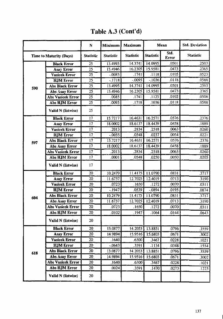
Table A.3 (Cont'd)

N Minimum Maximum Mean Std. Deviation

Time to Maturity (Days) Statistic Statistic Statistic Statistic Std. Statistic

Error

Black Error 25 13.4995 14.3741 14.0995 .0501 .2503

Asa:;r Error 25 15.4946 16.2305 15.9581 .0473 .2365

Vasicek Error 25 .. 0085 .1741 .1118 .()105 .0523

HJM Error 25 ·.1718 -.0095 -.1036 .OJ18 .0588

590 Abs Black Error 25 13.4995 14.3741 14.0995 .0501 .2503

Abs !t.say Error 25 15.4946 16.2305 15.9581 .0473 .2365

Abs Vasicek Error 25 .0085 .1741 .1125 .0102 .0508

Abs HJM Error 25 .0095 .1718 .1036 .0118 .0588

Valid N (listwise) 25

Black Error 17 15.7217 16.4631 16.2571 .0576 .2376 Asay Error 17 18.0002 18.6137 18.4439 .0458 .1889

Vasicek Error 17 .2013 .2834 .2518 .0063 .026{)

HJM Error 17 -.0055 .0548 .0237 .0054 .0221

S'YI Abs Black Error 17 15.7217 16.4631 16.2571 .0576 .2376 Abs Asay Error 17 18.0002 18.6137 18.4439 .0458 .1889

Abs Vasicek Error 17 .2013 .2834 .2518 .0063 .0260 Abs HJM Error 17 .0001 .0548 .0250 .0050 .0205

Valid N (listwise) 17

Black Error 20 10.2479 11.4175 11.0790 .083 I .3717 Asay Error 20 11.6737 12.7025 12.4019 .0713 .3190

Vasicek Error 20 .0723 .1650 .1272 .0070 .0311 HJM Error 20 -.1947 .0539 -.0894 .0195 .0874

604 Abs Black Error 20 10.2479 11.4175 11.0790 .0831 .3717 Abs Asay Error 20 11.6737 12.7025 12.4019 .0713 .3190

Abs Vasicek Error 20 .0723 .1650 .1272 .0070 .0311 Abs HJM Error 20 .0102 .1947 .!OM .0144 .0643

Valid N (Listwise) 20

Black Error 20 13.0877 14.2053 13.8851 .0796 .3559 Asay Error 20 14.9894 15.9516 15.6803 .0671 .3002

Vasicek Error 20 .1640 .6300 .3467 .0228 .1021 HJM Error 20 -.OM3 .3591 .I 134 .0348 .1554

618 Abs Black Error 20 13.0877 14.2053 13.8851 .0796 .3559 Abs Asay Error 20 14.9894 15.9516 15.6803 .0671 .3002

Abs Vasicek Error 20 .1640 .6300 .3467 .0228 .1021 Abs HJM Error 20 .0024 .3591 .1470 .0273 .1223

Valid N (listwise) 20

137

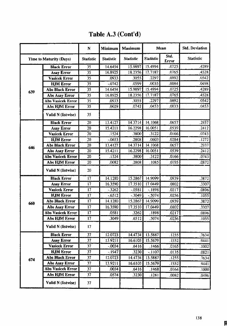
Table A.3 (Cont'd)

N Minimwn Maximum Mean Std. Deviation

Time to Maturity (Days) Statistic Statistic Statistic Statistic Std. Statistic

Error

Black Error 35 14.6454 15.9897 I 5.4994 .0725 .4289

Asay Error 35 16.8925 18.2356 17.7187 .0765 .4528

Vasicek Error 15 .0933 .3055 .2297 .0092 .0542

HJM Error 35 -.0742 .0599 .0035 .0084 .0498

639 Abs Black Error 35 14.6454 15.9897 15.4994 .0725 .4289

Abs Asay Erroo 35 16.8925 18.2356 17.7187 .0765 .4528

Abs Vasicek Error 35 .0933 .1055 .2297 .0092 .0542

Abs HJM Error 35 .0029 .0742 .0453 .0033 .0453

Valid N (listwise) 35

Black Error 20 13.4127 14.3714 14.1068 .0657 .2937

Asay Error 20 15.4211 16.2298 16.0051 .0539 .2412

Vasicek Error 20 .1524 .3800 .3122 .0166 .0743

HJM Error 20 -.0653 .2808 .0603 .0284 .1272

646 Abs Black Error 20 13.4127 14.3714 14.1068 .0657 .2937

Abs Asay Error 20 I 5.4211 16.2298 16.0051 .0539 .2412

Abs Vasicek Error 20 .1524 .3800 .3122 .0166 .0743

Abs HJM Error 20 .0082 .2808 .1085 .0195 .0872

Valid N (listwise) 20

Black Error 17 14.1280 15.2867 14.9099 .0939 .3872 Asay Error 17 16.3590 17.3510 17.0449 .0802 .3307

Vasicek Error 17 -.3262 -.0581 -.1898 .0217 .0896 HJM Error 17 -.6512 -.3049 -.5074 .0256 .1055

660 Abs Black Error 17 14.1280 15.2867 14.9099 .0939 .3872

Abs Asay Error 17 16.3590 17.3510 17.0449 .0802 .3307

Abs Vasicek Error 17 .0581 .3262 .1898 .0217 .0896

Abs HJM Error 17 .3049 .6512 .5074 .0256 .1055

Valid N (listwise) 17

Black Error 37 12.0723 14.4734 13.5887 .1255 .7634 Asay Error 37 13.9211 16.6103 15.5679 .1552 .9441

Vasicek Error 37 ·.0034 .6416 .1466 .CI65 .1002 IUM Error 37 -.1 S47 .3230 -.1107 .0135 .0821

674 Abs Black Error 37 12.0723 14.4734 13.5887 .1255 .7634 Abs Asay Error 37 13.9211 16.6103 15.5679 .1552 .9441

Abs Vasicek Error 37 .0034 .6416 .1468 .0164 .1000 Abs RJM Error 37 .0574 .3230 .1281 .0082 .0496

Valid N (listwise) 37

138

Table A.3 (Cont'd)

N Minimum Maximum Mean Std. Deviation

Statistic Statistic Stalistic Statistic Sid.

Statistic Time to Maturity (Days) Error

Black Error 17 14.7744 15.5305 15.3200 .0591 .2435

Asay Error 17 17.2565 17.8671 17.6996 .0459 .IH91

Vasicek Error 17 ·.0367 .1315 .()833 .0134 JJ553

HJM Error 17 ·.8540 ·.0416 ·.2223 .0419 .1727

681 Abs Black Error 17 14.7744 15.5305 15.321XJ .0591 .2435

Abs Asay Error 17 17.2565 17.8671 17.6996 .(J459 .1891

Abs Vasicek Error 17 .0100 .1315 .0888 .0110 .0453

Abs H.JM Error 17 .0416 .8540 .2223 .0419 .1727

Valid N (listwise) 17

Black Error 20 14.1026 14.9029 14.6870 .0531 .2376

Asay Error 20 16.3712 17.0319 16.8380 .0427 .1911

Vasicek Error 20 .1333 .4192 .3102 .0220 .0983

HJM Error 20 ·,0766 .3143 .0546 .0309 ,])g]

709 Abs Black Error 20 14.1026 14.9029 14.6870 .0531 .2376

Abs Asay Error 20 16.3712 17.0319 16.8380 .0427 .1911

Abs Vasicek Error 20 .1333 .4192 .3102 .0220 .0983

Abs HJM Error 20 .0090 .3143 .1131 .0209 .0935

Valid N (listwise) 20

Black Error 17 16.3977 17.1472 16.9354 .0590 .2431

Asay Error 17 19.3285 19.9244 19.7602 .0451 .1859

Vasicek Error 17 .2105 .2879 .2569 .0062 .0255

HJM Error 17 .0047 .0342 .0227 .0022 .0090

730 Abs Black Error 17 16.3977 17.1472 16.9354 .0590 .2431

Abs Asay Error 17 19.3285 19.9244 19.7602 .0451 .1859

Abs Vasicek Error 17 .2105 .2879 .2569 .0062 .0255

Abs HJM Error 17 .0047 .0342 .0227 .0(J22 .0090

Valid N (listwise) 17

Black Error 15 15.6338 16.4536 16.1976 .0714 .2766 Asay Error 15 18.3413 19.0117 18.8133 .0574 .2224

Vasicek Error 15 ·.2763 ·.0750 ·.1787 .0168 .0650

HJM Error 15 ·.6824 ·.3340 ·.5543 .0277 .1071

751 Abs Black Error 15 15.6338 16.4536 16.1976 .0714 .2766 Abs AsJay Error 15 18.3413 19.0117 18.8133 .0574 .2224

Abs Vasicek Error 15 .0750 .2763 .1787 .0168 .0650 Abs HJM Error 15 .3340 .6824 .5543 .0277 .1071

Valid N (listwise) 15

139

Table A.4

l>escriptive Statistics for CaU option.'i on 90-Day Bank Accepted BUII<'utures with different ranges of volatility

N Minimum Maximum Mean Std. Deviation

Ranges of volatility Statistic Statistic Statistic Statistic Std. Statistic

Error

Black Error 2 6.1736 1 1.0994 8.6365 2.4629 3.4H31

Asay Error 2 6.4327 1 1.9458 9.1892 2.7566 3.8984

Vasicek Error 2 .0316 .1046 .0681 JJJ65 JJS 16

HJM Error 2 -.0257 -.0143 -.0200 .rJOS7 .fXJH I

Missing Abs Black Error 2 6.1736 1 1.0994 8.6365 2.4629 3.4831 Values Abs Asay Error 2 6.4327 1 1.9458 9.1892 2.7566 3.8984

Abs Vasicek Error 2 .0316 .1046 .0681 .0365 .OS 16

Abs HJM Error 2 .0143 .0257 .0200 .0057 .0081

Valid N (listwi<e) 2

Black Error 53 -.0574 1.0882 .1873 .0411 .2991

Asay Error 53 -.0497 1.0980 .1966 .0413 .3006 Vasicek Error 53 -.0830 .2321 -.0014 .0078 .0570

HJM Error 53 -.0810 .1294 -.0103 .0052 .0382

0.05 toO.IO Abs Black Error 53 .0012 1.0882 .2069 .0392 .2857

Abs Asay Error 53 .0021 1.0980 .2129 .0397 .2891 Abs Vasicek Error 53 .0012 .2321 .0357 .0061 .0442

Abs RJM Error 53 .OOJJ .1294 .0285 .0037 .0271

Valid N (listwise) 53

Biack Error 75 -.0661 2.4926 .6185 .0651 .5642 Asay Error 75 -.0587 2.5418 .6388 .0658 .5695

Vasicek Error 75 -.3706 .3661 -.0698 .0192 .1659 HJM Error 75 -.3696 .2635 -.0890 .OIJS .IS I 7

0.11 toO.IS Abs Black Error 75 .0019 2.4926 .6264 .0641 .5554 Abs Asay Error 75 .0067 2.5418 .6455 .0649 .5619

Abs Vasicek Error 75 .0001 .3706 .1223 .0152 .1315 Abs HJM Error 75 .0015 .3696 .1171 .0151 .1309

Valid N (listwise) 75

Black Error 226 -.0207 4.9988 2.3394 .0774 1.1640 Asay Error 226 -.013 I 5.1722 2.4308 .0799 1.2018

Vasicek Error 226 -.4JJ8 .3923 .0077 .0107 .1603 HJM Error 226 -.4696 .2903 -.0329 .0093 .1400

0.!6to0.20 Abs Black Error 226 .0099 4.9988 2.3397 .0774 1.1634 Abs Asav Error 226 .0026 5.1722 2.4310 .0799 1.2015

Abs Vasicek Error 226 .0010 .4738 1139 .0075 .1128 Abs HJM Error 226 .0004 .4696 .0890 .0075 .I 12H

Valid N (listwise) 226

140

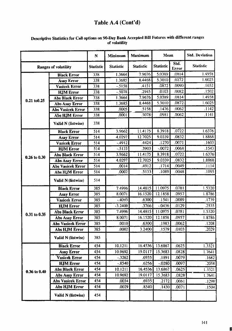
Table A.4 (Cont'd)

Descriptive Statistics for Call options on 90-Day Bank AccepWd Bill J<'utures wilh different ranges of volalilily

N Minimum Maximum Mean Std. Deviation

Ranges of volatility Statistic Statistic Statistic Statistic Std.

Statistic Error

Black Error 338 1.3664 7.9676 5.0389 .OHI4 1.4958

ASaV Error 338 1.3685 8.4468 5.3010 .o:m 1.6025

Vasicek Error 338 -.5158 .4151 .0872 .0090 .1652

lUM Error 338 -.5078 .2945 .0103 .(X\82 .1502

0.21 to0.25 Abs Black Error 338 1.3664 7.9676 5.0389 .0814 1.49Sg

Abs Asay Error 338 \.3685 8.4468 5.3010 .0872 1.6025

Abs Vasicek Error 338 .0005 .5158 .1476 .0062 .1142

Abs HJM Error 338 .0001 .5078 .0981 .0062 .1141

VaJid N (listwise) 338

Black Error 514 3.9662 11.4175 8.3918 .0722 1.6376

Asay Error 514 4.0297 12.7025 9.0339 .0832 1.8868

Vasicek Error 514 -.4912 .4424 .1270 .0071 .1603

HJMError 514 -.5133 .3903 -.0072 .0068 .1543

0.26 to 0.30 Abs Black Error 514 3.9662 11.4175 8.3918 .0722 1.6376

Abs Asay Error 514 4.0297 12.7025 9.0339 .0832 1.8868

Abs Vasicek Error 514 .0014 .4912 .1714 .0049 .1114

Abs HJM Error 514 .0002 .5133 .\089 .0048 .1095

Valid N (listwise) 514

Black Error 385 7.4996 14.4815 11.0975 .0781 1.5320

Asay Error 385 8.0071 16.1520 12.1858 .0957 1.8786

Vasicek Error 385 -.4D'i3 .6300 .1541 .0089 .1739

HJM Error 385 -3.2400 .3766 -.0436 .0129 .2535

0.31 to0.3S Abs Black Error 385 7.4996 14.4815 11.0975 .0781 1.5320

Abs Asav Error 385 8.0071 16.1520 12.1858 .0957 1.8786

Abs Vasicek Error 385 .0010 .6300 .1983 .0062 .1208

Abs HJM Error 385 .0002 3.2400 .1579 .0\03 .2029

Valid N (listwise) 385

Black Error 454 10.1211 16.4536 13.6867 .0625 1.3321 Asav Error 454 10.9692 19.0\17 15.3683 .0828 1.7641

Vasicek Error 454 -.3262 .6935 .1891 .0079 .1682

HJMError 454 -.8540 .6256 -.0280 .0097 .205K

0.36 to0.40 Abs Black Error 454 \0.1211 16.4536 136867 .0625 1.3321 Abs Asav Error 454 10.9692 19.0117 15.368] .0828 1.7641

Abs Vasicek Error 454 .0034 .6935 .2172 .0\)61 .1298 Abs HJM Error 454 .0029 .8540 .1430 .0071 .1504

Valid N (listwise) 454

141

II

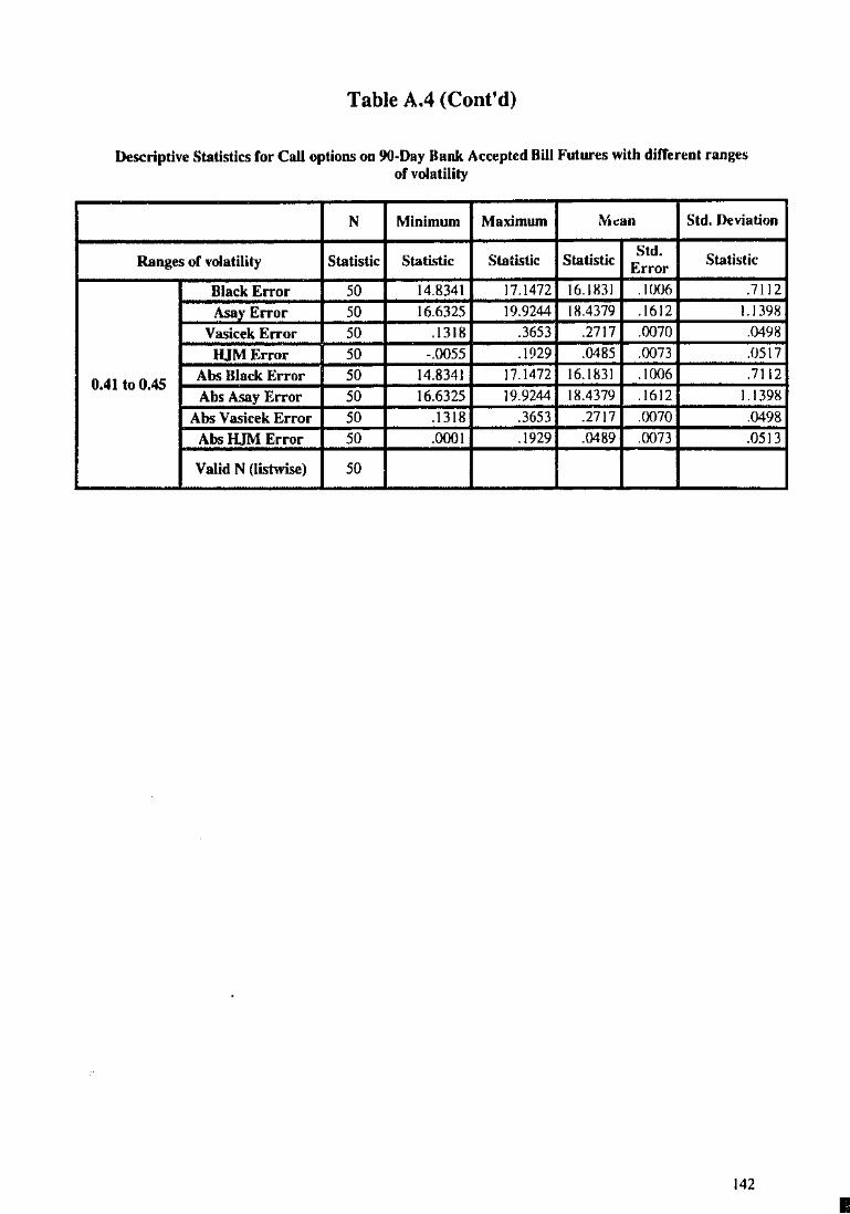
Table A.4 (Cont'd)

Descriptive Statistics for Call options on 90-Day Bank Accepted Bill Futures with different ranges of volatility

N Minimum Maximum M.:an Std. Deviation

Ranges of volatility Statistic Statistic Statistic Statistic I :::~r Statistic

~Error 5( 17.1472 :]:1831 . IIXJ6 .7112

I ~~;;:r 50 !.4379 16 1.1 398 5( .1318 .3653 .271 .0070 .0498

IIJM Error 50 -.0055 17 :ill .0485 .oc . )51

0.41 to o.45 :;':: 5C 14.8341 JII831 .1006 .7112

50 l.4379 .161 1398

Abs 'Error .1318

~ill 27r mm .0498

Abs I Error .0001 .0489 .00 .05

Valid N (listmse) 50

142

•

Table A.S

Descriptive Statistics for Call oplion.'i on 90-Uay Dank Ac~pted Bill Futures with different strike price

N Mio:!mwn Maximum Mean Std. Deviation

Strike Price Statistic Statistic Statistic Stati.'itic Std. Error Statistic

Black Error 5 -.0574 2.2085 1.0295 .4745 I .0609

Asay Error 5 -.CJ497 2.3384 1.1194 .5019 1.122]

Vasicek Error 5 -.2239 .(]]39 -.0743 .0405 .0905

HJM Error 5 -.2204 .0164 -.0723 .<!402 .OKY!J

88 Abs Black Error 5 .0193 2.2085 1.0602 .4572 1.0224

Abs Asay Error 5 .0200 2.33H4 1.1393 .4906 J.O<J70

Abs Vasicek Error 5 .0139 .2239 .0798 .0377 .0844

Abs HJM Error 5 .0164 .2204 .0788 .0370 .0827

Valid N (listwise) 5

Black Error 4 -.0467 2.2992 .8571 .5562 1.1123 Asay Error 4 -.0394 2.4260 .9248 .5825 1.1650

Vasicek Error 4 -.0722 .0139 -.0292 .0177 .0355 HJMError 4 -.0710 .0164 -.0277 .0181 .0361

88.25 Abs Black Error 4 .0091 2.2992 .8805 .5439 1.0877 Abs Asa_y Error 4 .0394 2.4260 .9445 .5719 1.1437

Abs Vasicek Error 4 .0139 .0722 .0361 .0128 .0256

Abs HJM Error 4 .0164 .0710 .0359 .0123 .0246

Valid N (listwise) 4

Black Error 15 -.0457 4.8961 1.5342 .4546 1.7606 Asay Error 15 -.0400 5.2270 1.6498 .4835 1.8724

Vasicek Error 15 ·.3706 .1177 -.0758 .0323 .1251 HJMError 15 -.3696 .1198 -.0741 .0321 .1245

88.50 Abs Blat!k Error 15 .0207 4.8961 1.5487 .4510 1.7469 Abs Asay Error 15 .0131 5.2270 1.6620 .4804 1.86()8

Abs Vasicek Error 15 .0096 .3706 .1052 .0258 .0998 Abs HJM Error 15 .0099 .3696 .1042 .0255 .0988

Valid N (listwise) 15

Black Error 32 -.0661 7.4996 2.5007 .4001 2.2635 Asay Error 32 -.0587 8.0071 2.6886 .4303 2.4344

Vusicek Error 32 ·.5158 .2499 -.0691 .0296 .1672 HJMError 32 -.5078 .2543 -.0658 .0301 .1701

88.75 A.Os Black Error 32 .0099 7.4996 2.5096 .3983 2.2533 Abs Asay Error 32 .0026 8.0071 2.6961 .4288 2.4258

Abs Vasicek Error 32 .0126 .5158 .1282 .0223 .1261 Abs HJM Error 32 .0102 .5078 .1290 .0225 .1274

Valid N (listwise) 32

143

Strike Price

Black Error Asay Error

k Error HJM Error

89 Abs Black Error Abs Asay Error

Abs · k Error Abs HJM Error

N

62 62 62 62 62 62 62 62

VaHd N (Ustwise) 62

Table A.S (Cont'd)

Minimum u

·.0549 ·.0479 ·.5 IS I ·.5078 .0133 .0202 .00](

.0032

3.4995 15.494!

.67

.62Sf 13.4995 15.494!

.671

Mean

· I Std. Error .5:

-.019 -.0371 5 i 143 6.0683

.1503

. 1441

.SHS

.026f

.025f

.52(

.585 I

~

Std. Deviation

4.J<Wi

4.61 I .zrm 2017

469% 4.6071

.1464

.1443

Black Error 7S -.0533 1~;+-...; 66;:.::._;.; .. 6771.;+-1,__.;·;::;:;503(+---.; 41..~4420 Asay Error 78 ~ 19.32Kl 7.3861 .5738 5.0675

IIJM ~~:;r ~: -~ .6243 .004 Ji~ .~

Valid N (Ustwise) 78

I--ll~ llack Error 83 -.0410 16.51 .5141 l.say Error 83 034 I~ .5898 5.37:fl

<Error 83 -5018 ~ .02 HJM Error 83 -.4978 .0: . 1929

89,50 A~ Error __ 83 015; 16.51 J: .232 .5 38 A~Error 83 .0100 8.027 .5895 5.mo

Abs 'Error 83 .0023 .680! .1512 .0153 .1397

Abs~~I~EErr~or-t~8~3-r--~-00~--~--6~059~~13~89 ___ ~-014~8-----~-111~,-Valid N (listwise) 83

144

I

Table A.S (Coot' d)

N Minimum Maximum Mean Std. Deviation

strike Price .7JITT IE:~ . ~:;::; 91 -. 37' 4.787

91 -.C 318 19.5191 8.6878 .5779 5.5m

I w~~~;:;r 91 -.4984 .6925 JJ4j7 .om .2091

91 -3.24(]( .601 .051' .0411 .39

8975 Abs~Error 91 .oo87 'Tim '3016 4.7R46

• -. y Error 91 .0040 19.5191 8.6890 .5777 5.5108

Abs~Error 91 .0016 .69: 1588 .0149 .1419

· Abs HJM Error 91 .0010 .178: .0369 .3521

Valid N (listwise) 91

Black Error 90 -.0232

19~ Ts6fs .5047 4.7883

Asay Error 90 -. )197 8.715: .5798

I UjS' I Er~::or 90 -.4830 .6899 ili99 -:om· .2112

90 -.48~ .58 -.0134 .0211 .2001

90 90 .0108

19]'&1

7:8625 3!)46

AbsAsav:S: JO 15 8.7161 .5796

; Error 90 .0026 .6899 'J650 .015; .1439

~ "ii:iM Error 90 .0021 .581: .1450 .0145 .1377

Valid N (listwise) 90

Black Error J3 -.0168 8.3272 .4894 4.7197

Asav Error J3 -.011: 19.681 9.2395 .5642 5~ 93 -.4746 .6935 mT .0216 HJMError 93 -.63: ;668 -.0210 .0217 .2093

90.25 AbsBlac~ 93 .010 8.32' .489: AbsAsay 93 .009 19.6815 .564T 5.44(1(

Abs '~ 93 .0001 .6935 .1655 .0153 .1478 I Error 93 .ooo9 .6328 .1488 .015 - .1478

Valid N (listwise) 93

~Error 94 -.0089 "'i6Z79s' .4875 4.7267 94 -.007 19.7434 9.3533 .5613 5.4417

~Error -.4619 5840 .0910 -:om .212( -.5680 m: -.01 .0208 -~

90.50 Abs •lack Error .0019 .4875 4.7 Abs wyError 94 .0067

~ 9~~ .5612 5.4414 Abs 'Error 94

..:ffi~ .0158 .153[ Abs::E!E Error 94 .5680 ~1457 .014: .1391

Valid N (listwise) 94

145

I

Table A.S (Cont'd)

N Minimwn Maximum Mean Std. l>eviation

Strike Price Statistic Statistic Statistk Statistk Std. Error Statistic

Black Error 94 -.0056 16.9454 8.5030 .4894 4.7447

Asay Error 94 -.tXl46 19.7958 9.3936 .5628 5.4562

Vasicek Error 94 -.4337 .6821 _1()49 .0210 .2034

HJM Error 94 -.6144 .5191 -.0111 .(}209 .2025

90.75 Abs Black Error 94 .0056 16.9454 8.5031 .4894 4.7445

Abs Asay Error 94 .0046 19.7958 9.3937 .5628 5.4561

Abs Vasicek Error 94 .0012 .6821 .1743 .0152 .1477

Abs HJM Error 94 .0003 .6144 .1450 .0145 .1410

Valid N (listwise) 94

Black Error 95 .0012 17.0014 8.5586 .4847 4.7246

Asay Error 95 .0021 19.8386 9.4343 .5573 5.4323

V a.sicek Error 95 -.4126 .6682 .1174 .0206 .2006

HJM Error 95 -.6544 .4881 -.0135 .0209 2039

91 Abs Black Error 95 .0012 17.0014 8.5586 .4847 4.7246

Abs Asay Error 95 . 0021 19.8386 9.4343 .5573 5.4323

Abs Vasicek Error 95 .0012 .6682 .1807 .0149 .1455 Abs lUM Error 95 .0013 .6544 .1453 .0147 .1428

Valid N (listwise) 95

Black Error 96 .0243 17.0578 8.6943 .4816 4.7186 Asay Error 96 .0250 19.8819 9.5678 .5531 5.4191

Vasicek Error 96 -.3967 .6530 .1297 .0199 .1946 HJMError 96 -.8540 .4571 -.0187 .0228 .2231

91.25 Abs Black Error 96 .0243 17.0578 8.6943 .4816 4.7186 Abs Asay Error 96 .0250 19.8819 9.5678 .5531 5.4191

Abs Vasicek Error 96 .0018 .6530 .1841 .0147 .1436 Abs HJM Error 96 .0020 .8540 .1549 .0164 .1609

Valid N (listwise) 96

Black Error 94 .0474 17.0945 8.6945 .4827 4.6799 Asay Error 94 .0480 19.9056 9.5373 .5535 5.3667

Vasicek Error 94 -.3716 .6369 .1468 .0195 .1893 HJM Error 94 -.6824 .4273 -.0143 .0212 .2051

91.50 Abs Black Error 94 .0474 17.0945 8.6945 .4827 4.6799 Abs Asay Error 94 .0480 19.9056 9.5373 .5535 5.3667

Abs Vasicek Error 94 .0018 .6369 .1947 .0143 .1390 Abs HJM Error 94 .0020 .6824 .1431 .0152 .1469

Valid N (listwise) 94

146

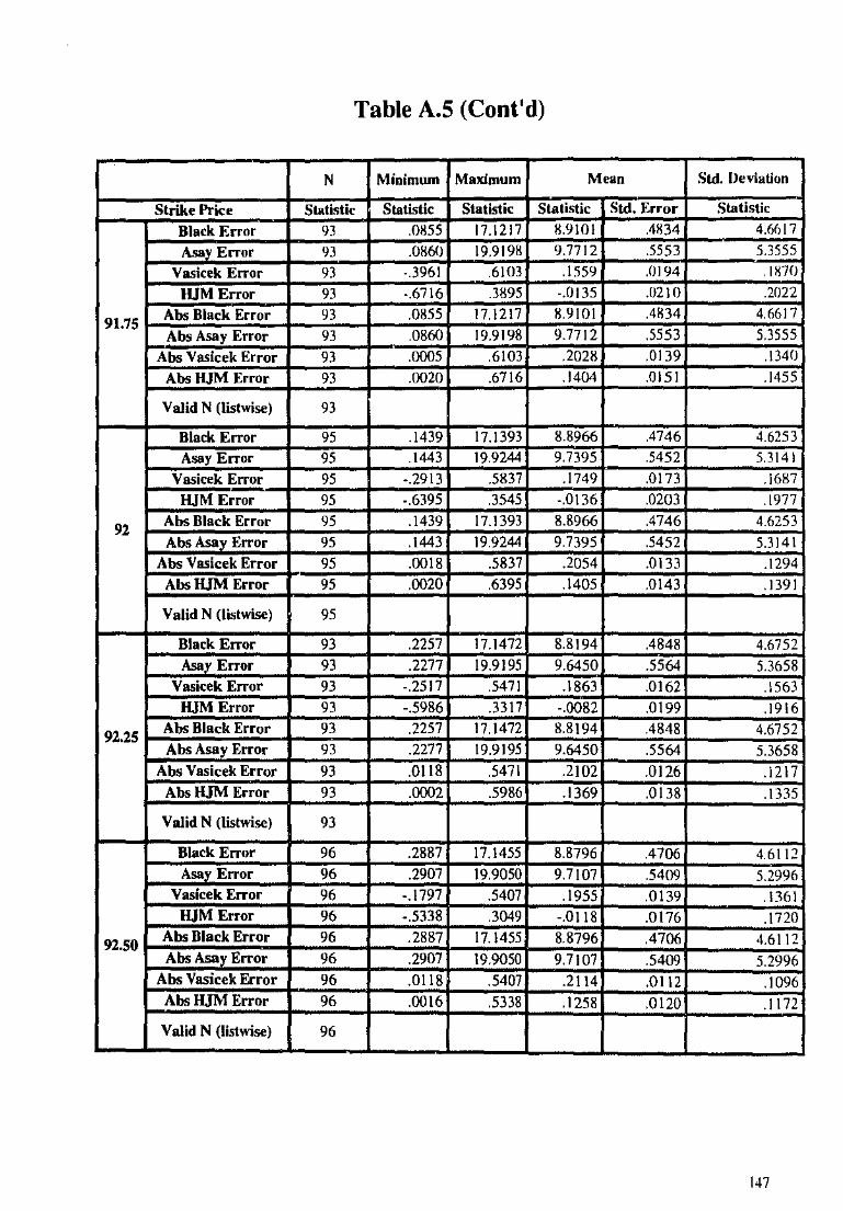
Table A.S (Cont'd)

N Minimwn Maximum Mean Std. Deviation

Strike Price Slatistic Statistic Statistic Statistic Std. Error Statistic

Black Error 93 .0855 17.1217 8.9101 .4834 4.6617

Asay Error 93 .0860 19.9198 9.7712 .5553 5.3555

Vasicek Error 93 -.3961 .6103 .1559 .0194 . I!S70

IUM Error 93 -.6716 .3895 -.0135 .0210 .2022

91.75 Abs Black Error 93 .0855 17.1217 8.9101 .4834 4.6617

Abs Asay Error 93 .0860 19.9198 9.7712 .5553 5.3555

Abs Vasicek Error 93 .0005 .6103 .2028 .0139 .\340

Abs HJM Error 93 .0020 .6716 .1404 .0151 .1455

Valid N (listwise) 93

Black Error 95 .1439 17.1393 8.8966 .4746 4.6253

Asay Error 95 .1443 19.9244 9.7395 .5452 5.3141

Vasicek Error 95 -.2913 .5837 .1749 .0173 .1687

HJM Error 95 -.6395 .3545 -.0136 .0203 .1977

92 Abs Black Error 95 .1439 17.1393 8.8966 .4746 4.6253

Abs A5!1y Error 95 .1443 19.9244 9.7395 .5452 5.3141

Abs Vasicek Error 95 .0018 .5837 .2054 .0133 .1294

Abs HJM Error 95 .0020 .6395 .1405 .0143 .1391

Valid N (listwise) 95

Black Error 93 .2257 17.1472 8.8194 .4848 4.6752

Asa___r_Error 93 .2277 19.9195 9.6450 .5564 5.3658 Vasicek Error 93 -.2517 .5471 .1863 .0162 .1563

HJM Error 93 -.5986 .3317 -.0082 .0199 .1916

92.25 Abs Black Error 93 .2257 17.1472 8.8194 .4848 4.6752 Abs Asay Error 93 .2277 19.9195 9.6450 .5564 5.3658

Abs Vasicek Error 93 .0118 .5471 .2102 .0126 .1217 Abs HJM Error 93 .0002 .5986 .1369 .0138 .1335

Valid N (listwise) 93

Black Error 96 .2887 17.1455 8.8796 .4706 4.6112 Asay Error 96 .2907 19.9050 9.7107 .5409 5.2996

Vasicek Error 96 -.1797 .5407 .1955 .0139 .1361 HJM Error 96 -.5338 .3049 -.0118 .0176 .1720

92.50 Abs Black Error 96 .2887 17.1455 8.8796 .4706 4.6112 Abs Asay Error 96 .2907 19.9050 9.7107 .5409 5.2996

Abs Vasicek Frror 96 .0118 .5407 .2114 .0112 .1096 Abs HJM Error 96 .0016 .5338 .1258 .0120 .1172

Valid N (listwise) 96

147

Table A.S (Cont'd)

N Minimum Maximum Mean Std. Deviation

Strike Price Statistic Statistic Statistic Statistic Std. Error 5tatistic

Black Error 92 .3635 17.1342 9.1684 .4597 4.409{)

Asay Error 92 .3654 19.8809 10.0105 .5303 5.0866

Vasicek Error 92 -.1065 .4746 .1896 .0124 .1193

HJM Error 92 -.4711 .2702 -.0154 .0157 .1502

92.75 Abs Black Error 92 .3635 17.1342 9.1684 .4597 4.4090

Abs Asay Error 92 .3654 19.8809 10.0105 .5303 5.0866

Abs Vasicek Error 92 .0014 .4746 .1997 .0105 .lOll

Abs IUM Error 92 .0004 .4711 .1121 .0105 .1005

Valid N (listwise) 92

Black Error 87 .4512 17.1133 9.5557 .4488 4.1860

Asay Error 87 .4528 19.8473 10.4358 .5203 4.8528

Vasicek Error 87 -.0955 .4386 .1907 .0107 .0998

IUM Error 87 -.4063 .2361 -.0245 .0134 .1250

93 Abs Black Error 87 .4512 17.1133 9.5557 .4488 4.1860

Abs Asay Error 87 .4528 19.8473 10.4358 .5203 4.8528

Abs Vasicek Error 87 .0035 .4386 .1951 .0098 .0910

Abs HJM Error 87 .0001 .4063 .0942 .0091 .0852

Valid N (listwise) 87

Black Error 85 .5524 17.0828 9.7139 .4479 4.1291 Asay Error 85 .5538 19.8042 10.6073 .5196 4.7904

Vasicek Error 85 -.0750 .4034 .1857 .0097 .0895

HJMError 85 -.3340 .1912 -.0241 .0114 .1051

93.25 Abs Black Error 85 .5524 17.0828 9.7139 .4479 4.1291 Abs Asay Error 85 .5538 19.8042 10.6073 .5196 4.7904

Abs Vasicek Error 85 .0166 .4034 .1893 .0089 .0817

Abs HJM Error 85 .0001 .3340 .0809 .0077 .0708

Valid N (listwise) 85

Black Error 74 .6576 16.3845 9.4873 .4330 3.7244

Asa:v Error 74 .6587 18.4818 10.3083 .5008 4.3077 Vasicek Error 74 -.0083 .4163 .1892 .0085 .0734 HJMError 74 -.1984 .2073 -.0182 .0098 .0847

93.50 Abs Black Error 74 .6576 16.3845 9.4873 .4330 3.7244 Abs Asay Error 74 .6587 18.4818 10.3083 .5008 4.3077

Abs Vasicek Error 74 .0083 .4163 .1894 .0085 .0728 Abs IUM Error 74 .0021 .2073 .0685 .0061 .0525

Valid N (listwise) 74

148

Table A.S (Cont'd)

N Minimum Maximum Mean Std. [)e,·iation

~=;~ Str~iBkeel~a Prckkic'~EE0rc::::or:::~~ 7~]:§~1.3~664~~ 115~ .. HH~I49~~9•.~3H667II~ Sldl.}2 E.4r~r3oOrHt=~J . 3.655

Asay Ercor 72 1.3685 17.9847 IO.IH9~ .4977 4.223 < Ercor 7 -.0444 .369 .169f _()(fJI .0773

HJMError 72 -.1882 .197f. IJI61 .<Xl'!l .0

93_75 1-..:;;:,: Abs<::..:;:: Bl•::::•k•:.,; EE;::.:.:::rror-+___,7;;-:+--!.'~-3664~-:'-::55 .. ~8149+-~ 9'~-386i+--;:;.;··43 la<DB __ ..;1;.o-·6 "'555:,;:.3 Abs Asay Error 72 1.3685 I 7.9847 10. I 89~ .4977 4.223

Abs <Error 7 .001 .369 .171( ~ .0744

r-'A~bss~=U~Ml~Error~r-~72-+-~-~~~5_..;-~1976+--'-~~d~IC~~~----~-04~95

Valid N (listwise) 72

r--t--~-;; k Ercor 6! 2.789: 1.7622 .~~ .3888 3.1348 Asay Ercor 65 2.8274 ~ •v.;.:,;:;::;+-..;.4;:!5::;:+50 __ ...;:3~.6686::.j

~~-~~~rror~=~~~joo~•ll#:c~~30111 ~~~~=8~3---~~5~'771 HJ~ ~or ( -.1691 .241( ~ ~ .0715

94 AbsBiack Error 65 ~-· 22 .~~ ~ 3.1348 AbsAsay_Error 65 2.8274 ~ ·"~ AJ)U 3.6686

65

Black Ercor 63 2.7901 15.70CX .3907 -3.IOT6 Asay Ercor _2!. 2.8264 I 7.8474 .4577 3.6331

<Error 63 ~3 ~ .1412 .0076 .0657 1--:-'"'iiJM'E.,.:.: I Error 63 -.IOZ' .2588 -.0187 .0078 .0618

94•25 A~Error 63 2.790 15.70CX 3.101( ~bs Asay Error 63 17.8474 .4577 3.6331

---~~~E~rror~~6~'4-~;,D5~3~~~~-~1414~~~~----~-0~WJ Abs~rror 6' -~ .047 =~---..;:;:::;; .043'3~7

Valid N (listwise) 63

1--f--::iii;;cl;'Error 58 10.3710 .4025 ~ Asay l<rcor 58 .3046 .4728 j,OW/

< Error 58 .0046 .2298 .1284 .0067 .05

149

Table A.S (Cont'd)

N Minimum Maximum Mean Std. l>eviation

Strike Price Statistic Statio;tic Statio;:tk Statistic Std. Error Statistic

Black Error 46 4.7959 I 5.5667 ](l.JHIJ .4272 2JW74

Asay Error 46 4.954H 17.6919 11.3074 .5054 3.4275

Vasicek Error 46 .0075 .1957 .IOH I 006H .0460

HJM Error 46 -.09H6 .0442 -.0157 .CXJ47 .rn11 Abs Black Error 46 4.7959 15.5667 10.3813 .4272 2.H974

94.75 17.6919 11.3074 .5054 3.4275 Abs Asay Error 46 4.9548

Abs Vasicek Error 46 .0075 .1957 .IOHI .0068 .()46()

Abs IUM Error 46 .0008 .0986 .0259 .0035 .0239

Valid N (listwise) 46

Black Error 34 5.0452 15.4957 10.3521 .4714 2.7488

Asay Error 34 5.1842 17.6099 I 1.2789 .5621 3.2774

Vasicek Error 34 .0045 .6416 .1107 .0175 .IOIH

HJM Error 34 -.0789 .3230 -.0047 .0108 .0630

95 Abs Black Error 34 5.0452 15.4957 10.3521 .4714 2.7488

Abs Asav Error 34 5.1842 17.6099 11.2789 .5621 3.2774

Abs Vasicek Error 34 .0045 .6416 .1107 .0175 .1018

Abs HJM Error 34 .0003 .3230 .0305 .0094 .0551

Valid N (listwise) 34

Black Error 8 4.9480 10.5417 8.1361 .7669 2.1690

Asay Error 8 5.0841 11.3940 8.6677 .8708 2.4630

Vasicek Error 8 .0567 .1270 .0958 .0104 .0296

lUMError 8 -.0457 .0144 -.0102 .0068 .0191

95.25 Abs Black Error 8 4.9480 10.5417 8.1361 .7669 2.1690 Abs Asay Error 8 5.0841 11.3940 8.6677 .8708 2.4630

Abs Vasicek Error 8 .0567 .1270 .0958 .0104 .0296 Abs HJM E;ror 8 .0037 .0457 .0159 .0050 .0141

Valid N (listwise) 8

Black Error 6 6.5418 10.4576 8.9357 .6738 1.6504 Asay Error 6 6.8200 11.3122 9.5734 .7728 1.8929

Vasicek Error 6 .0513 .1025 .0784 .0092 .0226 HJM Error 6 -.0282 .0026 -.0118 .0044 .0109

95.50 Abs Black Error 6 6.5418 10.4576 8.9357 .6738 1.6504 Abs Ass.y Error 6 6.8200 11.]122 9.5734 .7728 1.8929

Abs Vasicek Error 6 .0513 .1025 .0784 .0092 .0226 Abs HJM Error 6 .0026 .0282 .0127 .0039 .0096

Valid N (listwise) 6

150

Table A.S (Cont'd)

N Minimum Maximum Mean Std. Deviation

Strike Price Statistic Statistic Statistic Statistic Std. Error Statistic

Black Error 4 9.0678 10.3742 9.8625 .3010 .61120 Asay ErTor 4 9.7438 I 1.2211 10.6405 .3456 .6912

Vasicek Error 4 .0405 .0842 .0626 .0122 .0244 HJM Error 4 -.0193 -.0016 • .[)J 02 .()()36 .0072

95.75 Abs Black Error 4 9.0678 10.3742 9.8625 .3010 .61120 AOO Asay Error 4 9.7438 11.2211 10.6405 .3456 .6912

Abs Vasicek Error 4 .0405 .0842 .0626 .0122 .0244 Abs HJM Error ~ .0016 .0193 .0102 .0036 .0072

Valid N (listwise) 4

151

Table A.6

Descriptive Statistics for Call optioru; on 90-Day Bank Accepted Bill l<'utures for months January to llecember 1996

N Minimum Maximum

Date Statistic Statl'itic Statistic

Mean

Statistic Sid.

Error

Std. Deviation

Statistic

Black Error 174 .1159 H.626: .331 4 16BB A""Y Error 174 .14f 16.6103 9:5564 ~3iir 5.04B5

"iliM~~::r : ~: : ~~~ -~~~ -~~ -:o!f;~ ~~;11 3111196 ~~ Abs~s B~lack~' E~nr~orfj~~ 74~~~-~ 111~ 59~~144~_.47:i~ ,,~_6:_ 12~6:§~·33i_33 ~~~~~ 41~ .. 36B:~ Abs A""v Error 174 .I![ 9:5564 ~ 5.04H5

Abs <Error 174 .0034 .641 .1290 .U<J>J .0702

Abs ~::,;1 E~E'r:.:::,.ror+_:l~ 74+_..;:·000=:f--"' 3=2'f-:i':.:.;. TI;:.:.ifn+-'"J)(::::oo::::; ___ .;:: .. coq599

Valid N (listwise) 174

1---f--""iii;;cl;' Error 170 -.042~ 9.2224 .3937 5.13:

A""Y Error 170 -.04(){ !~ -~~- -:4448 5.799( <Error 170 -.0281 ~ ..;;,;:,::: 011: .1716

2Il/2/96 AbSiiia. 170 .0012 9.2251 .3933 5.1278 ~~~ffi~~IE~rror~~l7~0~~~---0~2~0~~-6~256~~~~-:oTI~Mif~~~-113~51 Abs """y Error 170 ~ . A#\ 5.7947 , Abs 'Error 170 ~ .6935 :Jm 0130 .1697

Abs HJM Error 170 .OOOT .6256 'irsT -:oT03 .1338

Valid N (listwise) 170

1---+--""iii;;cl;'Error 169 iJi76i .3745 4.8684

~rror 169 1.18: 19~ IT8023 .4400 5.7203 ~Error 169 ~ .2183 .0081 .10s;

2713196 ~; A~~bs~l~ Err~or~=~ :1 66~99 !:=~ ;;~~~662~=~171~ ~24:~~;~-~73~9=~3745 .004~6~=:-i-~0596~ ~"""vError 169 1.1827 19.92< 11.8023 .4400 ~

24/4196

Abs < Krror 169 .0016 .37~ .2196 .0079 . 1u,• ~ 169 .0015 .221 .0751 --:oo45 .0581

Valid N (listwise) 169

Black Error

~or Ab;As;f Error

Abs <Error Abs HJM Error

168 16 16 16 168 168 168 168

Valid N (listwise) \68

9.1644 17.8671 10~

.2910 .0844

.1929 ::Os3o 9.1647

!IE 10.1516 .29' .124( .854 .1002

.3669 Am

~ 3669 .4228 .005:

.1139

..:.!.222 4 7IT!! 5.4803 .0685 .0894

152

Table A.6 (Cont'd)

N Minimum Maximum Mean Std. Deviation

Date Statistic Statistic Statistic Statistic Std. Statistic

Jo:rrnr

Black Error 165 -.0574 14.4H15 H.7721 .3H41 4.1Jl4l

Asay Error 165 -.0497 16.1520 9.5951 .43 II 5.51K I

Vasicek Error 165 -.3961 .4151 .2327 .0103 131H

HJM Error 165 -.0449 .3113 .1261 .0062 .0794

29/5/96 Abs Black Error 165 .0087 14.4815 H.7754 .3H37 4.921Q

Abs Asay Error 165 .0040 16.1520 9.5978 .430H 5.5335

Abs Vasicek Error 165 .0049 .4151 .2405 .0092 .1179

Abs HJM Error 165 .0049 .3113 .1290 .0058 .0745

Valid N (listwise) 165

Black Error 157 .3711 15.1101 9.2829 .3523 4.4142

Asay Error 157 .4326 17.2445 10.1365 .4016 5.0325

Vasicek Error 157 -.0348 .3597 .1680 .0070 .(J874

HJM Error 157 -.1702 .2871 .0058 .0056 .0699

26/6/96 Abs Black Error 157 .3711 15.1101 9.2829 .3523 4.4142

Abs Asay Error 157 .4326 17.2445 10.1365 .4016 5.0325

Abs Vasicek Error 157 .0001 .3597 .1697 .0067 .()840

Abs lUM Error 157 .0013 .2871 .0539 .0036 .0447

Valid N (listwise) 157

Black Error 170 .0754 16.4536 8.4082 .3916 5.1064

Asay Error 170 .1075 19.0117 9.3364 .4538 5.9174

Vasicek Error 170 -.5158 .0856 -.2011 .0135 .1761

HJM Error 170 -.6824 -.0099 -.3793 .0132 .1725

3tn/96 Abs Black Error 170 .0754 16.4536 8.4082 .3916 5.1064

Abs Asay Error 170 .1075 19.0117 9.3364 .4538 5.9174

Abs Vasicek Error 170 .0010 .5158 .2155 .0121 .1581

Abs HJM Error 170 .0099 .6824 .3793 .0132 .1725

Valid N (listwise) 170

Black Error 182 -.0207 14.3714 H.3306 .3326 4.4865 Asay Error 182 -.0131 16.2298 9.1052 .3767 5.0818

Vasicek Error 182 -.1363 .3800 .0542 .0096 .\298

IUM Error 182 -.2383 .2808 -.0778 .0062 .0835

2818196 Abs Black Error 182 .0099 14.3714 8.3310 .3325 4.4859 Abs Asay Error 182 .0026 16.2298 9.1054 .3767 5.0815

Abs Vasicek Error 182 .0016 .3800 .1114 .0063 .0855 Abs IUM Error 182 .0001 .2808 .0971 .0044 .0599

Valid N (listwise) 182

153

Table A.6 (Coot' d)

N Minimum Maximum Mean Std. l>evi.ation

Date Statistic Statistic Slati'itic Stati!;tic Std.

Statistic l<:rror

Black Error IRJ 1.5851 14.9029 9.2874 .2945 3.9X32

Asay Error 183 1.6672 J7JBIIJ 10.2099 .3435 4.6467

Vasicek Error IRJ .11953 .6300 .3118 .(}073 .f1JK3

IUM Error 183 -.6328 .3903 .1724 JJ116 1569

2519196 Abs Black Error 183 1.585 I 14.9029 9.2874 .2945 3.9H32

Abs Asay Error 183 1.6672 17.0319 10.209'1 .3435 4.6467

Abs Vasicek Error 183 .0953 .6300 .3118 .1)()7 3 .0983 Abs HJM Error 183 .0005 .6328 .1925 .0097 .1313

Valid N (listwise) 183

Black Error 180 .5086 13.1192 7.405 I .2834 3.8020 Asay Error 180 .5430 14.8168 8.0921 .3226 4 3281

Vasicek Error 180 -.0990 .2577 .0753 .0074 .0994 HJM Error 180 -3.2400 .2410 -.0726 .0183 .2450

30/10/% Abs Black Error 180 .5086 13.1192 7.4051 .2834 3.8020 Abs Asay Error 180 .5430 14.8168 8.0921 .3226 4.3281

Abs Vasicek Error 180 .0010 .2577 .1008 .0055 .0733 Abs HJM Error 180 .0004 3.2400 .0807 .0181 .2424

Valid N (listwise) 180

Black Error 191 -.0661 11.4175 6.2950 .2582 3.5683 Asay Error 191 -.0587 12.7025 6.8267 .2874 3.9720

Vasicek Error 191 -.0482 .2051 .0821 .0046 .0633 HJM Error 191 -.1947 .1976 -.0122 .0048 .0667

271111% Abs Black Error 191 .0019 11.4175 6.2980 .2578 3.5628 Abs~y Erro:r 191 .0067 12.7025 6.8293 .2871 3.9675

Abs Vasicek Error 191 .0010 .2051 .0854 .0043 .0588 Abs HJM Error 191 .0016 .1976 .0502 .0033 .0455

Valid N (listwise) 191

Black Error 188 .8104 12.0372 7.6011 .2381 3.2652 Asay Error 188 .8895 13.1708 8.1678 .2621 3.5942

Vasicek Error 188 -.0897 .2869 .1197 .0081 .1106 HJM Ek·,~Jr 188 -.1095 .2588 -.0167 .0035 .0482

18112/96 Abs Black Error 188 .8104 12.0372 7.6011 .2381 3.2652 Abs Asay Error 188 .8895 13.1708 8.1678 .2621 3.5942

Abs Vasicek Error 188 .0005 .2869 .1355 .0066 .0905 Abs fUM Error 188 .0002 .2588 .0373 .0025 .0347

Valid N (listwise} 188

154

"' "'

i 0

!!; I Si ~

i

!j r--

::! ... ~ f 0

!= i I ti ~ ~

i ::! i i ~ 0 d

P; t:i !!; I ~I El SI ~ tE

s ~ ~

0 0 0

s~ -::i ~ts~

r--~ f:Fi ~~~ f:

i

j l

j

TA

BL

EA

.8 S

um

mary

labte fo, rM

at ~ p

ricing

error tor o

pU

on

• with d

lf'f•en

t drM

to fl\ab

llty M

d m

oneyneie•

Tim

e to

m•

. d

O

,,..., 11-00

11-120 121-1so

15

MIO

111-219

211-240 2

41

41

0

27

14

00

..,,_ .. ,.-H

1-H

O

301""'20 421-460 .. ,....,

411-610 611-640

Mt-670

571..«IO

00

1-'3

0

1131"870 8

71

-70

0

701-7'30 ,n

, lfc-0.02

1.1

46

7

1.4

91

5

2.1021 3

.18

ee 4.3330

5.117S

5.6467 t.5

79

6

7.0003 11.4115

l.82

t7

U3

06

10.8003

10

.e1ev

10.4037

12.-4673 12.51il64

11.82<40 1

3.7

&6

0

13.9920 12.7545

15.2338 14.2837

14.1337 1e.ee1•

141 131

m

C101 111)

{1151 (2

1)

1381 (1

4}

137' 1 ..

1 flt)

1461 11511

f,41) 1541

1301 f1

8)

1751 1341

1181 1361

1281 (111

1131 T

ffleto

.... cJO

J

l-00

.,...,

11

·12

0

121-150 1

i1•1

IO

111-210 2

11

44

0

24

14

70

2

71

40

0 --

.. ,..., ........ ,.,....., 421-460

46

1-

411-110 5

11

-64

0

141-670 1

71

..«IO

I0

1-'3

0

a, ... 1

0

171-700 701·7'30

,n1

-0.02dkD

.O:Z

0.319'4

T.7422

,..,.. 8.0022

8.2979 7

.20

H

7.5078 1.2721

I.CM

12 8 ......

10.2724 11.9961

10

.~

12.5253

U.3

70

9

10

.8""

13.1008 1

4.1

18

1

14

.32

10

17.06711

f1l 121

141 f1l

121 121

f1l f2l

141 121

111 121

121 121

111 111

121 131

111 111

Tim

• lo m

aa'"""'daY

• cJO

""""

.,..., 11-120

1'1

1-tlO

1

5M

IO

111""210 211-240

241-270 271-300

J0

14

30

3

'1-

H1-M

O

'91

....., 421-460 .. ,....,

411-110 511-640

Mt-1

70

5

71

«1

0

I01

-'30

131"870

971.700 7'01-7'30

>711 lb

0.0

2

0.2612 0.7474

1.I0

11

2

.4e6

7

3 . ....., 4.5204

5.1402 6.8340

e . .-ee1

1.1442 1.2315

7.0060 10.'4011

10.2209 9.M

110 12.2447

12.1731 1

1.1

I04

13.3511

13.7351 12.300,,4

14.7313 13.9723

14.5071 16.3171

1001 1531

15

n

CH

I 1ee1

1541 ,m

f102)

137' 1601

1711 (631

1 .. ,

.. ,, (731

1431 {521

,211 1 ..

, 1 ..

, 12-41

13'11 1201

191 1111

Tlr

n•to

ft'l.a

--•I

dO

.,...,

.,..., t1

-12

0

121•1IO

15

MIO

111-210

21

14

40

241•270

271-300 J

01

43

0

3'1

-- ........

.. 1.....,

421-460 4

61

-411-610

511-640 5

41

-17

0

571..«IO

eo

,.-821"

'70 171-700

701·7'30 >711

AIIM

0.2196

0.1202 1.9110

2.5733 3.8220

4.9602 5.3484

1.0512 1

.56

97

1.259'4

8.4646 e.o

n1

10.491!12

10.4151 10.1101

12

.3M

3

12.3783 11.3400

13.5788 13.&

670 12.4a20

14.973,4 14.133e

14.8870 18.S

496 1 ..

, 1581

1841 11031

(1061 1801

(107\ 11421

1521 1811

11211 1741

"'" 11201

f1241 1 ..

, 1921

1471 1421

1831 401

f72l 1541

1201 321

"-'"

T

im• to

ma

.... cJO

,,...,

., .... 1

1-1

20

121-150

15

MIO

111•210

211·240 241-270

27

14

00

J

01

43

0 .. ,.-

M1-M

O

111..UO

421-460 .. ,....,

411-610 1511-640

54

1-1

70

1

11

.eoo

0

01

.ac,

131-4170 471•700

701·7'30 >711

M<

-0.02 1.1-496

1.5023 2

.84

00

3.2-471

4.4475 5.2721

e.06

18

8.5706

7.4222 1.1857 ......

I.Hl3

1

11.4043 11.5002

11.2731 13.64611

13

.90

ee 12.7830

15.3416 15.7274

14.2-489 17.3082

11.3106 18.St297

19.15-448 141

(31 m

!10)

(111 1115)

128 1381

(141 137'

1 .. ,

t19l 1 ..

1 (51)

1411 1541

1391 1111

f751 1341

1111 1361

1281 f11l

1131 T

im• to

....

cJO

,,..., .,...,

11•120 1

21

·15

0

151-1IO

111-210 211•240

241-270 271-300

00

14

30

.. ,.-........

H1

....., 421-460 ..,....,

411-610 511-640

S4

t-l70

171..«IO

I0

1-'3

0

6:11-4170 ,1

1.7

00

701·7'30

,n1

-0.02<

Mdl.C

ll 0.3191

1.7543 3.5010

1.2

71

3

...... 7.5020

7.N

61

8.7.-cte

1.8

28

2

8.7

se1

11.0340 12.7131

11.38315 13.7264

15.9381 11.72M

I 14.5474

15.9689 18.2121

11.1119 111

121 141

Ill 121

121 f1l

(21 ,.,

(21 111

121 121

121 f1l

111 121

131 111

111 T

lrn•to

.. _l

dO

,,...,

.,..., 1

1-1

20

1'11•1IO

1

5M

IO

11

14

10

2

11

44

0

24

14

70

271-300

J0

14

30

3

'1

-M

14

IO

H1

....., 421-460 .. ,....,

411-110 111-640

M1

-17

0

171..«IO

eo1

.ac,

111-170 171•700

701.710 >711

M:,,0.02

0.2544 0.7817

1.6513 2

.56

52

3 .....

4.7

23

8

5.3981 1

.11

13

....... 8

.H1

1

e.1641 1

.41

73

11.2925

11

.1"8

1

0.n

09

13.5424

13.5751 12."'625

15.0041 15.5941

13.9028 1

1.H

N

18.1811 11.7259

19.1200 1001

1531 157'

1 .. 1

1ee1 1541

,m

11021 137'

(601 f7

1l

1531 1 ..

, 1871

1731 1431

(521 1211

1861 1481

1241 13'11

1201 191

1181 T

im• to

matu

"""'da"•

cJO

,,..., .,...,

t1-1

20

1

2M

S0

111-1IO

111-210

21

1·2

40

2

41

47

0

27

14

00

3

01

43

0

3'1

-H

14

IO .. ,.....,

421-460 .. ,...., 411-610

1511-640 5

41

-67

0

571..«IO

I01

-'30

831-4170

871•700 701-7'30

>711

..... 0.2927

0.1415 , .....

2.8681 3.7813

4.8

43

2

5.6932 8.38311

7.0381 e.7734

I.ON

1

1.8181 11.3450

11.3528 10.8711

13.8025 13.7-414

12.SU

O

15.11106 1

5.M

lt 1-4.0411

17.0831 11.2390

1e.aJ&O

19.31&

4 1 ..

1 /S

il 1841

11031 11051

flt! f10T

I 11421

(521 1801

f1211 f741

1031 11201

11241 1 ..

, 1921

1471 11421

1831 l""I

1721 1541

1201 1321

··-'"

_

. .. ..-...... ~ ......

Tim

• to m

a"--d

an

l cJO

""""

.,..., 1

1-1

20

121-1SO

1S

1•1IO

111-210 211•240

24

14

70

2

71

40

0

J0

14

30

3

'1--

>8141IO ,.,.....,

421-460 4&

1-41() 411-610

511-640 S

41-170 571..«IO

001.C

,O

131-170 671-700

701.710 >711

lik-0

.02

0.0600

0.1

2n

0.1147

0.2146 0.1724

0.2165 0

.20

63

0.14IO

0.2015

0.2012 0.1432

0.2t-<WI

0.1816 0.1687

0.1837 0.1722

0.1749 0.1738

0.1

80

8

0.154e 0.1901

0.2

03

0

0.19915 0

.23

80

O

.HK

IO

141 131

171 110\

1181 1151

1211 1381

1141 137'

1 .. ,

1111 1461

f511 f401

1541 1391

1111 (751

1341 1161

1361 1201

1111 f131

nm

.to

.... cJO

,,...,

.... ,o 11-120

121-150 111-1IO

111-210

211•240 241-270

27

14

00

0

01

43

0 .. ,.-

H1-M

O .. ,.....,

421-460 .. ,...., 411-610

511-640 1

41

-67

0

571..«IO

I01

-'30

831"

'70 871-700

701-710 ,n

, -0.C

ll<M

dl.02 0.0600

o.o

aeo

0 ...... 0.3084

0.3672 0.1803

0.4034 0.2790

0.2

0M

0.2321

0.1541 0.3718

0.2751 0.2430

0.3036 0.1597

0.2236 0.2046

0.3

44

6

0.2879 111

12 141

111 (21

121 1

121 141

121 111

121 121

121 111

11 121

13) Ill

111 n

m.to

ma

.... cJO

,,..,

.,..., 1

1-1

20

121-150

HM

IO

111-210 211-240

241•270 2

71

40

0

30

14

30

3'1-M

O ..,,..,., .. ,.....,

421-460 4

61

-411-110

511-640 S

,41-670 171..«IO

IO

I-GO

1

31

~7

0

171•700 701-7'30

>731 lb

G.0

2

0.0370 0.1331

0.0000 0

.08

90

0,1757

0.1708 0.1401

0.1752 0

.22

38

0.19157

9.1915 0.1121

0.208e 0.2491

0.1151 0.1961

0.1-443 0.2413

0.2178 9.1293

0.2M1

0.27&e

0.0

84

0

0.3085 0.2318

001 153

f571 IH

I eel

(541 im

1102)

(371 1601

171) (531

1 .. 1

187' 1731

431 (52)

28 1861

, .. , 1241

13'11 (201

,. (181

nm

. to

.... cJO

,,...,

.,..., tt-1

20

121-150

151-11() 111•210

211-240 241-270

27

14

00

..,,_ .. ,..., 311-M

O .. ,.....,

421-460 .. ,...., 411-610

511-640 5

41

-17

0

571..«IO

001-830 6:11-170

171-"TOO

701.710

,m

..... 0.0380

0.1312 0.1069

0.1

07

1

0.1784 0.1112

0.1112 o

.1eeo

0

.22

13

0.1199

0.17"le 0.1993

0.1917 0.2127

0.1196 0.1837

0.1

5N

0.21:M

0.1161

0.142-4 0.2389

0.2432 0.1215

0.3102 0.2202

, .. , 581

1841 (103}

(1051 1191

c1o

n

(1421 (521

1801 11211

174} 1031

(120) 112-4}

1 .. 1

1921 147'

/1-42) 1'31

1401 (7

2)

1541 (201

1321

n.,•; _

.._

,-,-...n-c

rrvr

Tim

• to m

a•u

•·-dily

• d

O

,,..., .,...,

11-120 121-1SO

1

6M

aJ

111-210 211-240

241-271 2

71

40

0

J0

14

30

3

'1--

)11--391 .. ,....., 421-460 .. ,....,

411-610 511-640

M1

-17

0

571.eoQ

001.C,O

1

31

~7

'0

871·700 701-731

>711

M<

-0.02 0

03

00

0 0520

0.0730 0

1() .

.

0.0

64

0

0.0700 0.0730

0.0470 0.0600

0.0710 0.0460

0.0410 0.0600

0.117-4 0

.04

30

0.0310

0.0

50

0

0.0870 0 0

99

0

0.0770 0.0960

00

99

0

0.130a 0.06-40

01

89

7

141 131

171 1101

,., 115

1281 138

f14l 1371

1 .. 1

1111 1 ..

, !11

1-491 154

1391 1181

75

341

1181 36

1281 111'

13 n

m. to

m•turttv(daly•

dO

.....

., .... 1

1•1

20

121-150

151-1IO

111-210 211-240

241-270 2

71

40

0

:IO

I-331-M

O

H1-M

O

>01-420

421-460 .. ,...., 411-610

15

11

~

5-41-67'0 571..«IO

001-030

&31-17'0

171-700 701-731

,n,

-0.02-cMc0.02

0.0300 0.0480

0.1

25

0

0.1-463 0.1805

0.1971 9.18711

0.1359 0.1415

0.0610 0.1278

0.1172 0.0340

0.1898 0 1112

0.17"1 0.1048

0.1048 0.0082

0.02t'O

"' 121

141 '

121 2

111 121

141 121

Ill 121

121 12

11 Ill

21 13

" l

nm

. to m

aturttvfdalH

<:IO

,,..., ......

81

·12

0

121·1SO

151-1IO

111-210

211-240 241-279

27

14

00

:IO

I- .. ,..., 301-390 ,.,.....,

421-460 .. ,...., 411-110

511-640 S

41-67'0 1571..«IO

001-G

O

6:11-17'0 171-100

701-TJO

,m

M

>0.02

0.03&0

0.1328 o.on,o

0.0

67

0

0.1827 0.1271

0.0970 0.1503

0.1664 0.1161

0.1963 0

.12

5e

0.1213 0.2405

o.1ooe 0.1212

0.1209 0.1515

0.1U36

0.1786 0.1478

0.2475 0.1&

M

0.1&54

0.34-49 100>

153 1571

1191 ...

1541 m

, 1021

1371 1601

/71

l 1531

1 .. ,

1871 173)

143> 521

128) 1861

1 .. ,

124) 13'1)

,,., 191

(18/ T

im• to

ma

.... cJO

,,...,

81-00 1

1-1

20

121-1SO

151•1IO

111-210

211-240 241•270

27

14

00

J

01

43

0 ,.,..., ........ ,.,.....,

421-460 .. ,...., 411-610

511-640 5

41

-67

0

571..«IO

001-GO

6:11-17'0

571.700 701·1:IO

>711

AIIM

0.0360

0 1257 0.0750

0.0TJO

0.14-40

0.1148 0.0020

0.1305 0.1371

0.0970 0.1364

0.1022 0.0060

0.1873 o.ono

0.1002 0.0030

0.1238 0.1423

0.13,4.3 0 1287

0.1720 0.1578

0.1131 0.2719

1 .. 1

1581 1841

(103) 11051

flt\ 1

10

n

11421 1521

119) 11211

1741 1031

11201 112-41

1 .. 1

1921 147'

11-421 1831

!40} (72\

1541 1201

1321

Noc•: T

h9 n...rnb41r of o

pP

'W w

ithin .act, e.t•g

ory

1• llhoM'I in b

racb

t.

156

DEFINITION OF TERMS

Gaussian Distribution The normal probability distribution. Its mathematical structure was developed by Carl Frederich Gauss ( 1777-1855) and the curve is often referred a<; the Gaussian distribution. The mathematical function that plots the normal curve has the following density function f(x) = _I_ e ·lt~·IJ.l/CIJ~ 2n

,j 21t where x is the value of the random variable, j.l is its expected value and cr is the standard deviation. Any normally distributed random variable can be expressed as a standard normal random variable by subtracting its expected value and dividing by its standard deviation. The standardized normal variable has the following function: f(x) = _I_ e ·•'"'

,j 21t The standard nonnal variable has expected value of zero, a variance of I and is synunctric.

Mean Reversion Interest rates do not typically drift upward or downward without encountering some resistance and a reversal of direction. The interest rate r responsible for the mean reversion can be seen as having an average drift or expected change, with volatility superimposed upon the drift. Mean reversion implies that the drift tends to pull interest back to some long­run average level. When the short-tenn interest rate is very high, r tends to have a negative drift; when the short-tenn interest rate is very low, r tends to have a positive drift. Mean reversion allows predictions about long-term interest rates. The volatility of a spot interest rate tends to be a decreasing function of its maturity. For example, the ten-year spot interest rate tends to have a lower volatility than the five-year spot interest rate; the five-year spot inter,;:st rate tends to have a lower volatility than the one-year spot interest rate etc.

Using the Vasicek model as an example, if the model assumes that the short rate follows the stochastic process of: dr : a(fl- r)dt + odW

where dr is a standard d Wiener process and r is the current level of the interest rate. )1 is the long run average interest rate. Jl is positive and is the rate at which the interest rate is pulled. If the current rate is higher (lower) than the long run average r > ( <)fl, the factor a (!l - r)dt induces negative (positive) expected change, which pulls the rate down (up) towards the average proportional to the factor dt, which is the length of time over which the change is observed.

crdW is a standard process for modelling uncertainty.

The coefficient Jl is the speed of adjustment of the interest rate towards its long run normal level. With this feature, interest rates could not drift permanently upward the way stock prices do.

157

Stochastic Process It is a sequence of observations from a probability distribution. Real world asset prices come from changing distributions though it is difficult to determine when a distrihution has changed. Empirical analysis of past data can be useful in predicting when the numbers arc coming out according to different bounds of probability.

Synchronous markets Galai ( 1983) describes the attributes of synchronous markets. Synchronous markets arc markets in which trading in related assets take place simultaneously and quoted prices reflect this simultaneity. Synchronization includes trading synchronization and data synchronization. Trading synchronization stands for parallel trading in two related securities. It is not sufficient for proving market syncluonization since data recording may be nonsynchronized. The technology for registration of trades must be such that the data accurately present the timing of the transaction and the time the infonnation is made available to market participants. If data on a class of options and the underlying stocks are used and the price quotes are not taken at the same time, based on parallel trading, the markets will appear to be nonsynchronous, though they may still be efficient.

White's Adjustments It tests whether the error variance is affected by any of the regressors, their squares or their cross products. It examines whether or not any heteroskedasticity present causes the variance-covariance matrix of the OLS estimator to differ from its usual formula.

Steps must be taken to calculate ~EGLs once the presence of heteroskedasticity has been confirmed. The first step in the process is to determine the functional fonn of the relationship determining the variance. The relationship is then estimated and used to fonn an estimate of the variance~covariance matrix G of the disturbance term. Using the estimate (G'), the estimator ~EGLS can be calculated.

An alternative way of calculating pEGLS can be used. This alternative way involves transforming the original equation to create an estimating relationship in transfonned variables that has spherical disturbances. The OLS estimator can then be applied to the transfonned data, producing the GLS estimator. In the case of heteroskedasticity, the appropriate transformation is obtained by dividing each observation by the square root of the estimated variance of the disturbance term.

Wiener Process If E(t) denotes a series of numbers coming out of a standard normal probability distribution and t denotes the point in time, the numbers are on average equal to zero and have a standard deviation of 1. The numbers are of the standard normal type. Taking any number and call it Z(t) at time. When moving ahead to time t+l and call it E(t+l), a transformation of the standard normal variable into the Z variable would be to add E(t+l) to Z(t) to get Z(t+l). The difference between Z(t+l) and Z(t) is denoted as dZ(t) which can be def:ned as dZ(t) = e(t) ..J dt and this is called a Wiener Process. When squaring the Wiener process, it becomes perfectly predictable. When multiplying the square root of the time interval dt by a

!58

I

standard normal random variable E(t), the tnmsformcd value is unpredictable but the expected value and its variance arc known. The expected value is zero. Using the rule that the variance of a constant times a random variable is the constant squared times the variance of the random variable, the variance is predicted to be dt. When the variable of interest is dZ(t)2 and the value of E(t) is drawn. E(t) can be multiplied by the square root of dt and the entire expression is squared. This becomes E(t)2 dt. The variance of the expression can be found by squaring dt and multiplying it by the variance of E(t)2

• By definition, all values of dtk where k > l are zero. This results in that the length of the time interval becomes so short that squaring it makes it shorter and effectively zero. The expected value of dZ(t) 2 is the expected value of E(t)2dt. This is dt times the expected value of E(t). Since the variance of any random variable x is defmed as E[x2

] - E[x]2 and when E(t) is a standard normal variable, Var[E(t)] = E[E(t) 2

] - E[E(t)J' = I. When E[E(t)] = 0, so E[E(t)] 2 = I. Since Var[dZ(t) 2] = 0

and E[dZ(t)2] = Z(t)2 = dt , therefore E[dZ(t)2

] = 1 * dt = dt. This shows that any variable with zero variance can be expressed as its expected value i.e. dZ(t)2 = dt

The process can be used to model stock price movements. Over the long run, stock prices go up or 'drift". The Wiener process does not drift but it is easy to make drift either upward or downward. The stock prices are random but with different volatilities. The Wiener process can be transformed to give different volatilities. It would be harder to forecast stock prices further into the future than nearby and stock prices are always positive.

t59

REFERENC~;s

Abken, P. A. ( 1993). Generalized method of moments tests of forward rate processes. Working Paper, 93-7. Federal Reserve Bank of Atlanta.

Amin, K. I. (Dec 1991 ). On the Computation of Continuous Time Option Prices Using Discrete Approximations. Journal of Financial and Quantitative Analysis, Vol26 No.4, 477-495.

Amin, K. I., and Bodurtha, J. N. (Spring 1995). Discrete-Time Valuation of American Options with Stochastic Interest Rates. The Review of Financial Studies, Yol.8 No.I, 193-234.

Amin, K. 1., and Jarrow, R. A. (1992). Pricing Options on Risky Assets in a Stochastic Interest Rate Economy. Mathematical Finance, Vol2, 217-238.

Amin, K. 1., and Morton, A (1994). Implied Volatility functions in arbitrage-free term structure models. Journal of Financial Ec0110mics, Vol 35, 141-180.

Amin, K.l., and Ng, V. K. (July 1993). Option Valuation with Systematic Stochastic Volatility, The Journal of Finance, Vol XLVlll No.3, 881-910.

Asay, M. R. (1982). A note on the design of commodity option contracts. Journal of Futures Market, Vol 52, 1-7.

Attari, M. (1996). An equilibrium jump-diffusion model for bond option prices. University of Iowa, Working Paper.

Attari, M. (1997). Models of the Term Structure of Interest Rates: A Survey. Derivatives and Financial Mathematics. Nova Science Publishers. 39-54.

Ball, C. A., and Torous, W. N. (1985). On jumps in common stock prices and their impact on call option pricing. Journal of Finance, Vol. 40, 155-173.

Bates, D. S. (1996). Jumps and stochastic volatility: Exchange rate processes implicit in PHLX Deutsche mark options. Review of Financial Studies, Vol. 9, 69-l 07.

Bates, D. S. (1996). Testing Option Pricing Models. Chapter 20, Handbook of Statistics 14, Edited by G. S. Maddala and C. R. Rao. North Holland, Amsterdam.

Bhattacharya, M. ( 1983). Transaction data tests of efficiency of the Chicago Board Options Exchange. Journal of Financial Economics, Vol. 12, 161-185.

Bjork, T. (1996). Interest Rate Theory CIME Lecture Notes. Department of Finance, Stockhohn School of Economics, Stockholm University, Sweden.

160

•

Bjork, T., Kabanov, Y., and Runggaldicr, W. (1995). Bond market structure in the presence of marked point processes. Submitted to Mathematical Finance.

Black, F. (1976). The Pricing of Commodity Contracts. Journal of Financial Economics, Vol3, 167·179.

Black, F. , Derman, E .. and Toy, W. (1990). A One-Factor Model of Interest Rates and Its Application to Treasury Bond Options. Financial Analyst Journal, Vol. 46, 33-39.

Black, F., and Scholes, M. (1973). The Pricing of Options and Corporate Liabilities. Journal of Political Economy, Vol 81, 637-654.

Boyle, P. (March 1988). A Lattice Framework for Option Pricing with Two State Variables. Journal of Financial and Quantitative Analysis, Vol. 23 No.I, 1 ~ 22.

Brace, A., and Hodgson, A. (1991). Index Futures options in Australia- An Empirical Focus on Volatility. Accounting and Finance, Vo121 No.2, 13-20.

Brace, A., and Hodgson, A. ( 1991 ). Index Futures Options in Australia - An Empirical Focus on Volatility. Accounting and Finance, Vol. 31 No. 2, 13-30.

Brenner, M., Courtadon, G., and Subrahmanyam, M. (Dec 1985). Options on the Spot and Options on Futures. Journal of Finance, Vol. 40, 1303-1317.

Brennan, M. J., and Schwartz, E. S. (1977). The Valuation of American put options. Journal of Finance, Vol. 32, 449-462.

Brennan, M. J., and Schwartz, E. S. ( 1979). A Continuous Time Approach to the Pricing of Bonds. Journal of Banking and Finance, Vol. 3, 133-155.

Brennan, M., and Schwartz, E. ( !982). An Equilibrium Model of Bond Pridng and a Test of Market Efficiency. Journal of Financial and Quantitative Analvsis, Vol 17, 301-329.

Broadie, M., and Detemple, J. (Winter 1996). American Option Valuation: New Bounds, Approximationsl and a Comparison of Existing Methods. The Review of Financial Studies, Voi.9No.4,1211-1250.

Brown, S. J., and Dybvig, P. H. ( 1986). The Empirical Implications of the Cox, Ingersoll, Ross theory of the tenn structure of interest rates. Journal of Finance, Vol 41, 617-630.

Brown, R. L., and Shevlin, T. J. (June 1983). Modelling Option Prices in Australia Using the Black-Scholes Model. Australian Journal of Management, Vo!8, 1-20.

t61

Brown, C. A., and Taylor, S.D. (1997). A test of the Asay model for pricing options 011 the SPI futures contract. Pacific-Basin Finance Joumal, Vol5 (1997), 579-594.

Buhler, W. (1990). Valuation of Bond Warrants. Review of Futures Market, Vol. 9, 612-636.

Buhler, W., Uhrig, M., Walter, U., and Weber, T. ( 1995). An Empirical Comparison of Alternative Models for Valuing Interest Rate Options. Working Paper, University Mannheim.

Cao, C. (1992). Pricing foreign currency options with stochar.;tic volatility. University of Chicago Working Paper.

Chan, K. C., K.arolyi, G. A., Longstaff, F. A., and Sanders, A. B. (1992). An Empirical Comparison of Alternative Models of the Short-Term Interest Rate. The Journal of Finance, Vol. XLVII, No.3, 1209-1227.

Chen, L. (1996a). Stochastic Mean and Stochastic Volatility- A Three-Factor Model of the Tenn Structure of Interest Rates and Its Applications in Derivative Pricing and Risk Management. Financial Markets, Institutions & Instruments, Vol. 5 No. I, 1-87.

Chen, L. (1996b). Understanding and Managing Interest Rate Risks. World Scientific.

Chen, R., and Scott, L. ( 1992). Pricing Interest Rate Options in a Two-Factor Cox­Ingersoll-Ross Model of the Term Structure. The Review of Financial Studies, Vol. 5 No.4, 613-636.

Chiras, D. P., and Manaster, S. ( 1978). The Infonnation Content of Options Prices and a Test of Market Efficiency. Joumal of Financial Economics, Vol6, 213-234.

Cox, C. 1., and Ross, S. A. (1976a). A Survey of Some New Results in Financial Option Pieing Theory. Journal of Finance, 31, 383-402.

Cox, C. 1., and Ross, S. A. (1976b). The Valuation of Options for Alternative Stochastic Processes. Journal of Financial Economics, Vol3, 145~166.

Cox, J., Ross, S., and Rubinstein, M. (Sep 1979). Option Pricing: A Simplified Approach. Journal of Financial Economics, Vol. 7, 229-263.

Cox, J., Ross, S., and Ingersoll, J. (1985). A Theory of the Tenn Structure of!nterest Rates. Econometrica, Vol. 53, 385-407.

Daz, S. R. (1995). Jump Diffusion Processes and the Bond Markets. Harvard Business School, Working Paper.

t62

Dietrich-Campbell, B., and Schwartz, E. S. ( 1986). Valuing debt options: empirical evidence. lou mal of Financial Economics. Vol. 16, 321 ~343.

Dothan, M. ( 1978). On the Term Structure of Interest Rates. Journal of Financial Economics, Vol?, 229-264.

Duffie, D., and Singleton, K. ( 1995). Modeling of term structures of defaultuble bonds. Working paper, Stanford University.

Eatwell, J., Milgate M., and Newman, P. (1990). The New Palgrave: Time Series and Statistics. The Macmillan Press Ltd.

Evnine, J, and Rudd, A. (1985). Index options: The early evidence. Journal of Finance, Vol. 40,743-756.

Feller, W. (1951). Two Singular Diffusion Problems. Annal of Mathematics, Vol. 54, 173-182.

Flesaker, B. (1993) Testing the Heath-Jarrow-Morton!Ho-Lee Model of Interest Rate Contingent Claims Pricing. Journal of Financial and Quantitative Analysis, Vol. 28 No.4, 483-495.

Galai, D. (1983). A Survey of Empirical Tests of Option Pricing Models. In Brenner, M. , Options Pricing Theory and Application (Chapter 3). Lexington Books.

Gay, G., and Manaster, S. ( 1986). Implicit Delivery Options and Optimal Delivery Strategies for Financial Futures Contract. Journal of Financial Economics, Vol.16, 41-72.

Gibbons, MR., and Ramaswamy, K (1993). A Test of the Cox, Ingersoll, and Ross Model of the Term Structure. Review of Financial Studies, Vol. 6, 619-658.

Hair, J. F., Anderson, R. E., and Tatham, R. L. ( 1987). Multivariate Data Analysis. Macmillan Publishing Company, Second Edition.

Hawkins, G. D. ( 1982). An Analysis of Revolving Credit Agreements. Journal of Financial Economics, Vol. 10, 59-81.

Heath, D., !arrow, R.A., and Morton, A. (Dec 1990). Bond Pricing and the Term Structure of Interest Rate: A Discrete Time Approximation. Journal of Financial and Quantitative Analysis, Vol. 25. No.4, 419-440.

Heath, D., !arrow, R.A., and Morton, A. (1991). Contingent Claim Valuation with a Random Evolution of Interest Rates. Review of Futures Market, Vol. 9 No.I, 54-76.

16]

Heath, D., Jarrow, R.A., and Morton, A. (Jan 1992). Bond Pricing and the Term Structure of Interest Rates: A New Methodology For Contingent Claims Valuation. Econometrica, Vol. 60 No .1, 77-105.

Hedge, S. (1988). An Empirical Analysis of Implicit Delivery Options in the Treasury Bond Futures Contract. Journal of Banking and Finance, Vol. 12, 469-492.

Heston, S. (1993). A Closed Form Solution for Options with Stochastic Volatility with Applications to Bond and Currency Options. Review of Financial Studies, Vol. 6 No. 2.

Ho, T., and Lee, S. (Dec 1986). Term Structure Movements and Pricing of Interest Rate Contingent Claims. Journal of Finance, Vol. 41, 1011-1029.

Huang, J., and Yu, G. G. (Spring 1996). Pricing and Hedging American Options: A Recursive Integration Method. The Review of Financial Studies, Vol. 9 No.1, 277-300.

Hull, J. ( 1993). Options, Futures, and Derivative Securities. Prentice Hall, Second Edition.

Hull, J. ( 1995). Introduction to Futures and Options Markets. Prentice Hall. Second Edition.

Hull, J., and White, A. (Mar 1987). The Pricing of Options on Assets with Stochastic Volatilities. Journal of Finance, 281-300.

Hull, J., and White, A. (Sep 1988). The Use of the Control Variate Technique in Option Pricing. Journal of Financial and Quantitative Analysis, Vol. 23 No. 3, 237-251.

Hull, J., and White, A. (1990a). Pricing Interest Rate Derivatives Securities. Review of Financial Studies, Vol 3 No.4, 573-592.

Hull, J., and White, A. (1990b). Valuing Derivative Securities Using the Explicit Finite Difference Method. Journal of Financial and Quantitative Analysis, Vol. 25, 87-100.

Hull, J., and White, A. (1993). One-factor Interest-Rate Models and the Valuation of Interest-Rate Derivative Securities. Journal of Financial and Quantitative Analysis, Vol. 28, No. 2, 235-253.

Hull, J., and White, A. (Spring 1996). Using Hull-White Interest Rate Trees. The Journal of Derivatives, 26-36.

Jamshidian, F. ( 1991 ). Forward Induction and Construction of Yield Curve Diffusion Models. Journal of Fixed Income, Vol. l, 62-74.

164

Jarrow, R. A. (l 994). Derivative Security Markets, Market Manipulation, and Option Pricing Theory. Journal of Financial and Quantitative Analysis, Vol. 29 No. 2, 241-26 l.

Jarrow, R. A. (l 996). Modelling Fixed Income Securities and Interest Rate Options. McGraw-Hill.

Jarrow, R. A., Lando, D., and Turnbull, S. M. (1995). A Markov model for the term structure of credit risk spreads. To appear in Review of Financial Studies.

Jarrow, R. A., and Madan, D. (l 995). Option pricing using the Term Structure of Interest Rates to hedge systematic discontinuities in Asset Returns. Mathematical Finance, Vol 5, 311-336.

Jarrow, R. A., and Turnbull, S. ( 1995).Pricing Derivatives on Financial Securities Subject to Credit Risk. Journal of Finance, Vol. 50 No. l, 53-86.

Kennedy, P. ( 1992). A Guide to Econometrics. Basil Blackwell Ltd, Third Edition.

Kraus, A., and Smith, M. (June 1993). A Simple Multi-factor Term Structure Model. Journal of Fixed Income, 19-23.

Langetieg, T. C. (1980). A Multivariate Model of the Term Structure. Journal of Finance, Vol. 35, 71-97.

Latane, H., and Rendleman, R. J. (May 1976). Standard Deviation of stock price ratios implied by option premia. Journal of Finance, Vol 31, 369-382.

Lieu, D. (1990). Option Pricing with Futures-style Margining. Journal of Futures Market, Vol 10, 327-338.

Longstaff, F. ( 1989). A Non-linear General Equilibrium Model of the Term Structure of Interest Rates. Journal of Financial Economics, Vol. 23, 95-224.

Longstaff, F. and Schwartz, E. (Dec 1992 ). Interest Rate Volatility and the Term Structure: A Two Factor General Equilibrium Model. Journal of Finance, Vol. 47 No. 4, 1259-1282.

Longstaff, F. and Schwartz, E. (Sep 1993 ). Implementation of the Longstaff-Schwartz Interest Rate Model. Journal of Fixed Income, 7-14.

Melino, A. and Turnbull, S. M. ( 1990). Pricing foreign currency options with stochastic volatility. Econometrics, Vol 45, 239-265.

165

Merton, R. (1976). Option Pricing When Underlying Stock Return Are Continuous. Journal of Financial Economics, 125-144.

Miltersen, K.R., Sandmann, K., and Sondermann, D. ( 1997). Closed Form Solutions for Term Structure Derivatives with Log-Normal Interest Rates. The Journal of Finance, Vol. VII, No. 1, 409-413.

Myers, R. J.; and Hanson, S. D. (1993 ). Pricing Commodity Options when the underlying Futures Price exhibits time-varying volatility. Amer. J. Agricult. Econom, Vol 75, 121-130.

Nelson, D., and Ramaswamy, K. (1990). Simple Binomial Processes as Diffusion Approximations in Financial Models. Review of Financial Studies, Vol. 3 No.1, 393-430.

Ogden, J. P., and Tucker, A. L. (Dec 1988). The Relative Valuation of American Currency Spot and Futures Options: Theory and Empirical Tests. Journal of Financial and Quantitative Analysis, Vol. 23 No. 4, 351-368.

Platen, E. ( 1996). Explaining Interest Rate Dynamics. Preprint. Centre for Financial Mathematics, Australian National University, Canberra.

Ramanathan, R. (1993). Statistical Methods in Econometrics. Academic Press, Inc.

Ramaswamy, K., and Sundaresan, S. (Dec 1985). The Valuation of Options on Futures Contract. Journal of Finance, Vol. 40, 1319-1340.

Rendleman, R. J., Jr, and Barter, B. J. (March 1980). The Pricing of Options on Debt Securities. Journal of Financial and Quantitative Analysis, Vol. XV No. l, 11-24.

Richard, S. E. (March 1978). An Arbitrage Model of the Term Structure of Interest Rates. Journal of Financial Economics, Vol. 6, 33-57.

Ritchken, P., and Boenawan, K. (1990). On Arbitrage-free Pricing of Interest Rate Contingent Claims. Journal of Finance, Vol 45, 259-164.

Ritchken, P., and Sankarasubramanian, L. (Fall 1995). A Multifactor Model of the Quality Option in Treasury Futures Contracts. The Journal of Financial Research, Vol. XVIII No.3, 261-279.

Roger, L.C.G. ( 1995). Which model for term-structure of interest rates should one use? Mathematical Finance, Vol. 65, 93-116.

166

Schaefer, S. M., and Schwartz, E. S. (Dec 1984). A Two-Factor Model of the Term Structure: An Approximate Analytical Solution. Journal of Financial and Quantitative Analysis, Vol. 19 No.4, 413-423.

Schaefer, S. M., and Schwartz, E. S. (1987). Time-Dependent Variance and the Pricing of Bond Options. Journal of Finance, Vol. 42, 1113-1128.

Sheikh, A. M. (Dec 1991). Transaction Data Tests of S & P 100 Call Option Pricing. Journal of Financial and Quantitative Analysis, Vol 26 No. 4, 459-475.

Shirakawa, H. ( 1991 ). Interest rate options pricing with Poisson-Gaussian forward rate curve processes. Mathematical Finance, Vol. 1, 77-94.

Sidney, S., and Castellan, N. J. (1988). Nonparametric Statistics for the Behavioral Sciences. McGraw-Hill, Second Edition.

Stokes, H.H. ( 1997). Specifying and Diagnostically Testing Econometric Models. Quorum Books, Second Edition.

Turnbull, S. M., and Milne, F. (1991). A Simple Approach to Interest Rate Option Pricing. Review of Financial Studies, Vol. 4 No.1, 87-120.

Turnbull, S. M., and Wakeman, L. M. (Sep 1991). A Quick Algorithm for Pricing European Average Options. Journal of Financial and Quantitative Analysis, Vol. 26. No. 3, 377-389.

Vasicek, 0. (Nov 1977). An Equilibrium Characterization of the Term Structure. Journal of Financial Economics, Vol. 5, 177-188.

Whaley, R.E. (1982). Valuation of American Call Option on Dividend-Paying Stock: Empirical Tests. Journal of Financial Economics, Vol 10, 29-58.

White, K. J. (1997). Shazam: The Econometrics Computer Program, Version 8.0. McGraw­Hill.

167

-_,.-~?; .

:_) I_: 3 C-j(fl

J.iV!f

EDITH COWAN UNIVERSITY

11111111111 AA5243281B

7 DAY

LOAN