An Empirical Comparison of Voting Classi cation …ai.stanford.edu/~ronnyk/vote.pdf · An Empirical...
38
Machine Learning, vv, 1–38 (1998) c 1998 Kluwer Academic Publishers, Boston. Manufactured in The Netherlands. An Empirical Comparison of Voting Classification Algorithms: Bagging, Boosting, and Variants ERIC BAUER [email protected] Computer Science Department, Stanford University Stanford CA. 94305 RON KOHAVI [email protected] Data Mining and Visualization, Silicon Graphics Inc. 2011 N. Shoreline Blvd, Mountain View, CA. 94043 Received 3 Oct 1997; Revised 25 Sept 1998 Editors: Philip Chan, Salvatore Stolfo, and David Wolpert Abstract. Methods for voting classificationalgorithms, such as Bagging and AdaBoost, have been shown to be very successful in improving the accuracy of certain classifiers for artificial and real- world datasets. We review these algorithms and describe a large empirical study comparing several variants in conjunction with a decision tree inducer (three variants) and a Naive-Bayes inducer. The purpose of the study is to improve our understanding of why and when these algorithms, which use perturbation, reweighting, and combination techniques, affect classification error. We provide a bias and variance decompositionof the error to show how different methods and variants influence these two terms. This allowed us to determine that Bagging reduced variance of unstable methods, while boosting methods (AdaBoost and Arc-x4) reduced both the bias and variance of unstable methods but increased the variance for Naive-Bayes, which was very stable. We observed that Arc-x4 behaves differently than AdaBoost if reweighting is used instead of resampling, indicating a fundamental difference. Voting variants, some of which are introduced in this paper, include: pruning versus no pruning, use of probabilistic estimates, weight perturbations (Wagging), and backfitting of data. We found that Bagging improves when probabilistic estimates in conjunction with no-pruningare used, as well as when the data was backfit. We measure tree sizes and show an interesting positive correlation between the increase in the average tree size in AdaBoost trials and its success in reducing the error. We compare the mean-squared error of voting methods to non-voting methods and show that the voting methods lead to large and significant reductions in the mean-squared errors. Practical problems that arise in implementing boosting algorithms are explored, including numerical instabilities and underflows. We use scatterplots that graphically show how AdaBoost reweights instances, emphasizing not only “hard” areas but also outliers and noise. Keywords: Classification, Boosting, Bagging, Decision Trees, Naive-Bayes, Mean-squared error 1. Introduction Methods for voting classification algorithms, such as Bagging and AdaBoost, have been shown to be very successful in improving the accuracy of certain classifiers for artificial and real-world datasets (Breiman 1996b, Freund & Schapire 1996, Quinlan 1996). Voting algorithms can be divided into two types: those that adaptively change the distribution of the training set based on the performance of previous classifiers (as in boosting methods) and those that do not (as in Bagging).
Transcript of An Empirical Comparison of Voting Classi cation …ai.stanford.edu/~ronnyk/vote.pdf · An Empirical...

Machine Learning, vv, 1–38 (1998)c© 1998 Kluwer Academic Publishers, Boston. Manufactured in The Netherlands.
An Empirical Comparison of Voting ClassificationAlgorithms: Bagging, Boosting, and Variants
ERIC BAUER [email protected]
Computer Science Department, Stanford UniversityStanford CA. 94305
RON KOHAVI [email protected]
Data Mining and Visualization, Silicon Graphics Inc.2011 N. Shoreline Blvd, Mountain View, CA. 94043
Received 3 Oct 1997; Revised 25 Sept 1998
Editors: Philip Chan, Salvatore Stolfo, and David Wolpert
Abstract. Methods for voting classificationalgorithms, such as Bagging and AdaBoost, have beenshown to be very successful in improving the accuracy of certain classifiers for artificial and real-world datasets. We review these algorithms and describe a large empirical study comparing severalvariants in conjunction with a decision tree inducer (three variants) and a Naive-Bayes inducer.The purpose of the study is to improve our understanding of why and when these algorithms, whichuse perturbation, reweighting, and combination techniques, affect classification error. We providea bias and variance decompositionof the error to show how different methods and variants influencethese two terms. This allowed us to determine that Bagging reduced variance of unstable methods,while boosting methods (AdaBoost and Arc-x4) reduced both the bias and variance of unstablemethods but increased the variance for Naive-Bayes, which was very stable. We observed thatArc-x4 behaves differently than AdaBoost if reweighting is used instead of resampling, indicatinga fundamental difference. Voting variants, some of which are introduced in this paper, include:pruning versus no pruning, use of probabilistic estimates, weight perturbations (Wagging), andbackfitting of data. We found that Bagging improves when probabilistic estimates in conjunctionwith no-pruning are used, as well as when the data was backfit. We measure tree sizes and showan interesting positive correlation between the increase in the average tree size in AdaBoost trialsand its success in reducing the error. We compare the mean-squared error of voting methods tonon-voting methods and show that the voting methods lead to large and significant reductions inthe mean-squared errors. Practical problems that arise in implementing boosting algorithms areexplored, including numerical instabilities and underflows. We use scatterplots that graphicallyshow how AdaBoost reweights instances, emphasizing not only “hard” areas but also outliers andnoise.
Keywords: Classification, Boosting, Bagging, Decision Trees, Naive-Bayes, Mean-squared error
1. Introduction
Methods for voting classification algorithms, such as Bagging and AdaBoost, havebeen shown to be very successful in improving the accuracy of certain classifiers forartificial and real-world datasets (Breiman 1996b, Freund & Schapire 1996, Quinlan1996). Voting algorithms can be divided into two types: those that adaptivelychange the distribution of the training set based on the performance of previousclassifiers (as in boosting methods) and those that do not (as in Bagging).
2 ERIC BAUER AND RON KOHAVI
Algorithms that do not adaptively change the distribution include option decisiontree algorithms that construct decision trees with multiple options at some nodes(Buntine 1992b, Buntine 1992a, Kohavi & Kunz 1997); averaging path sets, fannedsets, and extended fanned sets as alternatives to pruning (Oliver & Hand 1995);voting trees using different splitting criteria and human intervention (Kwok &Carter 1990); and error-correcting output codes (Dietterich & Bakiri 1991, Kong &Dietterich 1995). Wolpert (1992) discusses “stacking” classifiers into a more com-plex classifier instead of using the simple uniform weighting scheme of Bagging. Ali(1996) provides a recent review of related algorithms, and additional recent workcan be found in Chan, Stolfo & Wolpert (1996).
Algorithms that adaptively change the distribution include AdaBoost (Freund& Schapire 1995) and Arc-x4 (Breiman 1996a). Drucker & Cortes (1996) andQuinlan (1996) applied boosting to decision tree induction, observing both thaterror significantly decreases and that the generalization error does not degradeas more classifiers are combined. Elkan (1997) applied boosting to a simple Naive-Bayesian inducer that performs uniform discretization and achieved excellent resultson two real-world datasets and one artificial dataset, but failed to achieve significantimprovements on two other artificial datasets.
We review several voting algorithms, including Bagging, AdaBoost, and Arc-x4,and describe a large empirical study whose purpose was to improve our under-standing of why and when these algorithms affect classification error. To ensurethe study was reliable, we used over a dozen datasets, none of which had fewer than1000 instances and four of which had over 10,000 instances.
The paper is organized as follows. In Section 2, we begin with basic notation andfollow with a description of the base inducers that build classifiers in Section 3.We use Naive-Bayes and three variants of decision tree inducers: unlimited depth,one level (decision stump), and discretized one level. In Section 4, we describethe main voting algorithms used in this study: Bagging, AdaBoost, and Arc-x4.In Section 5 we describe the bias-variance decomposition of error, a tool that weuse throughout the paper. In Section 6 we describe our design decisions for thisstudy, which include a well-defined set of desiderata and measurements. We wantedto make sure our implementations were correct, so we describe a sanity check wedid against previous papers on voting algorithms. In Section 7, we describe ourfirst major set of experiments with Bagging and several variants. In Section 8,we begin with a detailed example of how AdaBoost works and discuss numericalstability problems we encountered. We then describe a set of experiments for theboosting algorithms AdaBoost and Arc-x4. We raise several issues for future workin Section 9 and conclude with a summary of our contributions in Section 10.
2. Notation
A labeled instance is a pair 〈x, y〉 where x is an element from space X and y isan element from a discrete space Y . Let x represent an attribute vector with nattributes and y the class label associated with x for a given instance. We assumea probability distribution D over the space of labeled instances.
EMPIRICAL COMPARISON OF BOOSTING, BAGGING, AND VARIANTS 3
A sample S is a set of labeled instances S = {〈x1, y1〉, 〈x2, y2〉, . . . , 〈xm, ym〉}. Theinstances in the sample are assumed to be independently and identically distributed(i.i.d.).
A classifier (or a hypothesis) is a mapping fromX to Y . A deterministic induceris a mapping from a sample S, referred to as the training set and containing mlabeled instances, to a classifier.
3. The Base Inducers
We used four base inducers for our experiments; these came from two families ofalgorithms: decision trees and Naive-Bayes.
3.1. The Decision Tree Inducers
The basic decision tree inducer we used, called MC4 (MLC++ C4.5), is a Top-Down Decision Tree (TDDT) induction algorithm implemented inMLC++ (Kohavi,Sommerfield & Dougherty 1997). The algorithm is similar to C4.5 (Quinlan 1993)with the exception that unknowns are regarded as a separate value. The algorithmgrows the decision tree following the standard methodology of choosing the bestattribute according to the evaluation criterion (gain-ratio). After the tree is grown,a pruning phase replaces subtrees with leaves using the same pruning algorithmthat C4.5 uses.
The main reason for choosing this algorithm over C4.5 is our familiarity withit, our ability to modify it for experiments, and its tight integration with multiplemodel mechanisms withinMLC++. MC4 is available off the web in source form aspart ofMLC++ (Kohavi, Sommerfield & Dougherty 1997).
Along with the original algorithm, two variants of MC4 were explored: MC4(1)and MC4(1)-disc. MC4(1) limits the tree to a single root split; such a shallow treeis sometimes called a decision stump (Iba & Langley 1992). If the root attributeis nominal, a multi-way split is created with one branch for unknowns. If the rootattribute is continuous, a three-way split is created: less than a threshold, greaterthan a threshold, and unknown. MC4(1)-disc first discretizes all the attributesusing entropy discretization (Kohavi & Sahami 1996, Fayyad & Irani 1993), thuseffectively allowing a root split with multiple thresholds. MC4(1)-disc is very similarto the 1R classifier of Holte (1993), except that the discretization step is based onentropy, which compared favorably with his 1R discretization in our previous work(Kohavi & Sahami 1996).
Both MC4(1) and MC4(1)-disc build very weak classifiers, but MC4(1)-disc isthe more powerful of the two. Specifically for multi-class problems with continuousattributes, MC4(1) is usually unable to build a good classifier because the treeconsists of a single binary root split with leaves as children.
4 ERIC BAUER AND RON KOHAVI
3.2. The Naive-Bayes Inducer
The Naive-Bayes Inducer (Good 1965, Duda & Hart 1973, Langley, Iba &Thompson 1992), sometimes called Simple-Bayes (Domingos & Pazzani 1997),builds a simple conditional independence classifier. Formally, the probability of aclass label value y for an unlabeled instance x containing n attributes 〈A1, . . . , An〉is given by
P(y | x)= P(x | y) · P(y)/P(x) by Bayes rule∝ P(A1, . . . , An | y) · P(y) P (x) is same for all label values.
=n∏j=1
P(Aj | y) ·P(y) by conditional independence assumption.
The above probability is computed for each class and the prediction is madefor the class with the largest posterior probability. The probabilities in the aboveformulas must be estimated from the training set.
In our implementation, which is part of MLC++ (Kohavi, Sommerfield &Dougherty 1997), continuous attributes are discretized using entropy discretiza-tion (Kohavi & Sahami 1996, Fayyad & Irani 1993). Probabilities are estimatedusing frequency counts with an m-estimate Laplace correction (Cestnik 1990) asdescribed in Kohavi, Becker & Sommerfield (1997).
The Naive-Bayes classifier is relatively simple but very robust to violations ofits independence assumptions. It performs well for many real-world datasets(Domingos & Pazzani 1997, Kohavi & Sommerfield 1995) and is excellent at han-dling irrelevant attributes (Langley & Sage 1997).
4. The Voting Algorithms
The different voting algorithms used are described below. Each algorithm takesan inducer and a training set as input and runs the inducer multiple times bychanging the distribution of training set instances. The generated classifiers arethen combined to create a final classifier that is used to classify the test set.
4.1. The Bagging Algorithm
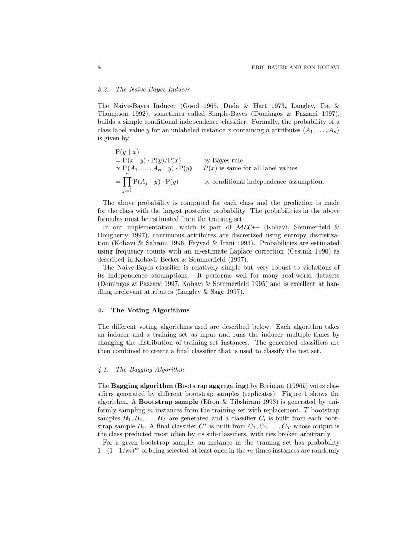
The Bagging algorithm (Bootstrap aggregating) by Breiman (1996b) votes clas-sifiers generated by different bootstrap samples (replicates). Figure 1 shows thealgorithm. A Bootstrap sample (Efron & Tibshirani 1993) is generated by uni-formly sampling m instances from the training set with replacement. T bootstrapsamples B1, B2, . . . , BT are generated and a classifier Ci is built from each boot-strap sample Bi. A final classifier C∗ is built from C1, C2, . . . , CT whose output isthe class predicted most often by its sub-classifiers, with ties broken arbitrarily.
For a given bootstrap sample, an instance in the training set has probability1−(1−1/m)m of being selected at least once in the m times instances are randomly
EMPIRICAL COMPARISON OF BOOSTING, BAGGING, AND VARIANTS 5
Input: training set S, Inducer I, integer T (number of bootstrap samples).
1. for i = 1 to T {
2. S′ = bootstrap sample from S (i.i.d. sample with replacement).
3. Ci = I(S′)
4. }
5. C∗(x) = arg maxy∈Y
∑i:Ci(x)=y
1 (the most often predicted label y)
Output: classifier C∗.
Figure 1. The Bagging Algorithm
selected from the training set. For large m, this is about 1 − 1/e = 63.2%, whichmeans that each bootstrap sample contains only about 63.2% unique instancesfrom the training set. This perturbation causes different classifiers to be built ifthe inducer is unstable (e.g., neural networks, decision trees) (Breiman 1994) andthe performance can improve if the induced classifiers are good and not correlated;however, Bagging may slightly degrade the performance of stable algorithms (e.g.,k-nearest neighbor) because effectively smaller training sets are used for trainingeach classifier (Breiman 1996b).
4.2. Boosting
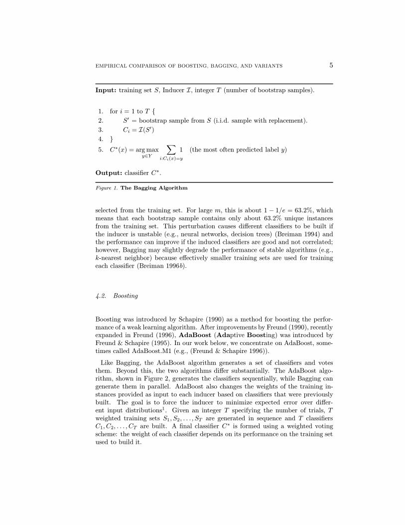
Boosting was introduced by Schapire (1990) as a method for boosting the perfor-mance of a weak learning algorithm. After improvements by Freund (1990), recentlyexpanded in Freund (1996), AdaBoost (Adaptive Boosting) was introduced byFreund & Schapire (1995). In our work below, we concentrate on AdaBoost, some-times called AdaBoost.M1 (e.g., (Freund & Schapire 1996)).
Like Bagging, the AdaBoost algorithm generates a set of classifiers and votesthem. Beyond this, the two algorithms differ substantially. The AdaBoost algo-rithm, shown in Figure 2, generates the classifiers sequentially, while Bagging cangenerate them in parallel. AdaBoost also changes the weights of the training in-stances provided as input to each inducer based on classifiers that were previouslybuilt. The goal is to force the inducer to minimize expected error over differ-ent input distributions1. Given an integer T specifying the number of trials, Tweighted training sets S1, S2, . . . , ST are generated in sequence and T classifiersC1, C2, . . . , CT are built. A final classifier C∗ is formed using a weighted votingscheme: the weight of each classifier depends on its performance on the training setused to build it.

6 ERIC BAUER AND RON KOHAVI
Input: training set S of size m, Inducer I, integer T (number of trials).
1. S′ = S with instance weights assigned to be 1.
2. For i = 1 to T {
3. Ci = I(S′)
4. εi = 1m
∑xj∈S′:Ci(xj)6=yj
weight(x) (weighted error on training set).
5. If εi > 1/2, set S′ to a bootstrap sample from S with weight 1 forevery instance and goto step 3 (this step is limitedto 25 times after which we exit the loop).
6. βi = εi/(1− εi)
7. For-each xj ∈ S′, if Ci(xj) = yj then weight(xj) = weight(xj) · βi.
8. Normalize the weights of instances so the total weight of S′ is m.
9. }
10. C∗(x) = arg maxy∈Y
∑i:Ci(x)=y
log1
βi
Output: classifier C∗.
Figure 2. The AdaBoost Algorithm (M1)
The update rule in Figure 2, steps 7 and 8, is mathematically equivalent to thefollowing update rule, the statement of which we believe is more intuitive:
For-each xj, divide weight(xj) by 2εi if Ci(xj) 6= yj and 2(1− εi) otherwise (1)
One can see that the following properties hold for the AdaBoost algorithm:
1. The incorrect instances are weighted by a factor inversely proportional to theerror on the training set, i.e., 1/(2εi). Small training set errors, such as 0.1%,will cause weights to grow by several orders of magnitude.
2. The proportion of misclassified instances is εi, and these instances get boostedby a factor of 1/(2εi), thus causing the total weight of the misclassified instancesafter updating to be half the original training set weight. Similarly, the correctlyclassified instances will have a total weight equal to half the original weight, andthus no normalization is required.
The AdaBoost algorithm requires a weak learning algorithm whose error isbounded by a constant strictly less than 1/2. In practice, the inducers we useprovide no such guarantee. The original algorithm aborted when the error boundwas breached, but since this case was fairly frequent for multiclass problem with
EMPIRICAL COMPARISON OF BOOSTING, BAGGING, AND VARIANTS 7
the simple inducers we used (i.e., MC4(1), MC4(1)-disc), we opted to continuethe trials instead. When using nondeterministic inducers (e.g., neural networks),the common practice is to reset the weights to their initial values. However, sincewe are using deterministic inducers, resetting the weights would simply duplicatetrials. Our decision was to generate a Bootstrap sample from the original data Sand continue up to a limit of 25 such samples at a given trial; such a limit was neverreached in our experiments if the first trial succeeded with one of the 25 samples.
Some implementations of AdaBoost use boosting by resampling because theinducers used were unable to support weighted instances (e.g., Freund & Schapire(1996)). Our implementations of MC4, MC4(1), MC4(1)-disc, and Naive-Bayessupport weighted instances, so we have implemented boosting by reweighting,which is a more direct implementation of the theory. Some evidence exists thatreweighting works better in practice (Quinlan 1996).
Recent work by Schapire, Freund, Bartlett & Lee (1997) suggests one explanationfor the success of boosting and for the fact that test set error does not increase whenmany classifiers are combined as the theoretical model implies. Specifically, thesesuccesses are linked to the distribution of the “margins” of the training exampleswith respect to the generated voting classification rule, where the “margin” of anexample is the difference between the number of correct votes it received and themaximum number of votes received by any incorrect label. Breiman (1997) claimsthat the framework he proposed “gives results which are the opposite of what wewould expect given Schapire et al.’s explanation of why arcing works.”
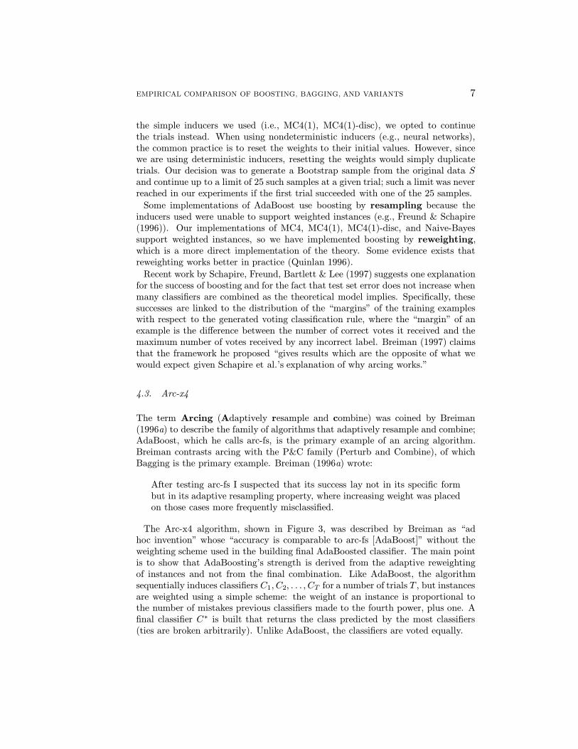
4.3. Arc-x4
The term Arcing (Adaptively resample and combine) was coined by Breiman(1996a) to describe the family of algorithms that adaptively resample and combine;AdaBoost, which he calls arc-fs, is the primary example of an arcing algorithm.Breiman contrasts arcing with the P&C family (Perturb and Combine), of whichBagging is the primary example. Breiman (1996a) wrote:
After testing arc-fs I suspected that its success lay not in its specific formbut in its adaptive resampling property, where increasing weight was placedon those cases more frequently misclassified.
The Arc-x4 algorithm, shown in Figure 3, was described by Breiman as “adhoc invention” whose “accuracy is comparable to arc-fs [AdaBoost]” without theweighting scheme used in the building final AdaBoosted classifier. The main pointis to show that AdaBoosting’s strength is derived from the adaptive reweightingof instances and not from the final combination. Like AdaBoost, the algorithmsequentially induces classifiers C1, C2, . . . , CT for a number of trials T , but instancesare weighted using a simple scheme: the weight of an instance is proportional tothe number of mistakes previous classifiers made to the fourth power, plus one. Afinal classifier C∗ is built that returns the class predicted by the most classifiers(ties are broken arbitrarily). Unlike AdaBoost, the classifiers are voted equally.
8 ERIC BAUER AND RON KOHAVI
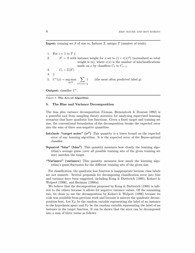
Input: training set S of size m, Inducer I, integer T (number of trials).
1. For i = 1 to T {
2. S′ = S with instance weight for x set to (1 + e(x)4) (normalized so totalweight is m), where e(x) is the number of misclassificationsmade on x by classifiers C1 to Ci−1.
3. Ci = I(S′)
4. }
5. C∗(x) = arg maxy∈Y
∑i:Ci(x)=y
1 (the most often predicted label y)
Output: classifier C∗.
Figure 3. The Arc-x4 Algorithm
5. The Bias and Variance Decomposition
The bias plus variance decomposition (Geman, Bienenstock & Doursat 1992) isa powerful tool from sampling theory statistics for analyzing supervised learningscenarios that have quadratic loss functions. Given a fixed target and training setsize, the conventional formulation of the decomposition breaks the expected errorinto the sum of three non-negative quantities:
Intrinsic “target noise” (σ2) This quantity is a lower bound on the expectederror of any learning algorithm. It is the expected error of the Bayes-optimalclassifier.
Squared “bias” (bias2) This quantity measures how closely the learning algo-rithm’s average guess (over all possible training sets of the given training setsize) matches the target.
“Variance” (variance) This quantity measures how much the learning algo-rithm’s guess fluctuates for the different training sets of the given size.
For classification, the quadratic loss function is inappropriate because class labelsare not numeric. Several proposals for decomposing classification error into biasand variance have been suggested, including Kong & Dietterich (1995), Kohavi &Wolpert (1996), and Breiman (1996a).
We believe that the decomposition proposed by Kong & Dietterich (1995) is infe-rior to the others because it allows for negative variance values. Of the remainingtwo, we chose to use the decomposition by Kohavi & Wolpert (1996) because itscode was available from previous work and because it mirrors the quadratic decom-position best. Let YH be the random variable representing the label of an instancein the hypothesis space and YF be the random variable representing the label of aninstance in the target function. It can be shown that the error can be decomposedinto a sum of three terms as follows:

EMPIRICAL COMPARISON OF BOOSTING, BAGGING, AND VARIANTS 9
Error =∑x
P (x)(σ2x + bias2
x + variancex)
(2)
where
σ2x ≡
1
2
1−∑y∈Y
P (YF = y|x)2
bias2
x ≡1
2
∑y∈Y
[P (YF = y|x) − P (YH = y|x)]2
variancex ≡1
2
1−∑y∈Y
P (YH = y|x)2
.
To estimate the bias and variance in practice, we use the two-stage samplingprocedure detailed in Kohavi & Wolpert (1996). First, a test set is split from thetraining set. Then, the remaining data, D, is sampled repeatedly to estimate biasand variance on the test set. The whole process can be repeated multiple timesto improve the estimates. In the experiments conducted herein, we followed therecommended procedure detailed in Kohavi & Wolpert (1996), making D twice thesize of the desired training set and sampling from it 10 times. The whole processwas repeated three times to provide for more stable estimates.
In practical experiments on real data, it is impossible to estimate the intrinsicnoise (optimal Bayes error). The actual method detailed in Kohavi & Wolpert(1996) for estimating the bias and variance generates a bias term that includes theintrinsic noise.
The experimental procedure for computing the bias and variance gives similarestimated error to holdout error estimation repeated 30 times. Standard deviationsof the error estimate from each run were computed as the standard deviation of thethree outer runs, assuming they were independent. Although such an assumptionis not strictly correct (Kohavi 1995a, Dietterich 1998), it is quite reasonable givenour circumstances because our training sets are small in size and we only averagethree values.
6. Experimental Design
We now describe our desiderata for comparisons, show a sanity check we performedto verify the correctness of our implementation, and detail what we measured ineach experiment.
6.1. Desiderata for Comparisons
In order to compare the performance of the algorithms, we set a few desiderata forthe comparison:

10 ERIC BAUER AND RON KOHAVI
18
20
22
24
26
28
30
32
0 500 1000 1500 2000 2500 3000 3500 4000 4500 5000
Err
or (
%)
Number of instances
waveform-40
MC4naive-bayes
12
14
16
18
20
22
24
0 1000 2000 3000 4000 5000 6000 7000
Err
or (
%)
Number of instances
satimage
MC4naive-bayes
10
15
20
25
30
35
40
0 2000 4000 6000 8000 10000 12000 14000 16000 18000 20000
Err
or (
%)
Number of instances
letter
MC4naive-bayes
26
28
30
32
34
36
38
40
42
0 500 1000 1500 2000 2500 3000 3500
Err
or (
%)
Number of instances
led24
MC4naive-bayes
2
4
6
8
10
12
14
16
18
0 500 1000 1500 2000 2500
Err
or (
%)
Number of instances
segment
MC4naive-bayes
72
73
74
75
76
77
78
79
0 500 1000 1500 2000 2500
Err
or (
%)
Number of instances
segment
Figure 4. Learning curves for selected datasets showing different behaviors of MC4 and Naive-Bayes. Waveform represents stabilization at about 3,000 instances; satimage represents a cross-over as MC4 improves while Naive-Bayes does not; letter and segment (left) represent continuousimprovements, but at different rates in letter and similar rates in segment (left); LED24 representsa case where both algorithms achieve the same error rate with large training sets; segment (right)shows MC4(1), which exhibited the surprising behavior of degrading as the training set size grew(see text). Each point represents the mean error rate for 20 runs for the given training set sizeas tested on the holdout sample. The error bars show one standard deviation of the estimatederror. Each vertical bar shows the training set size we chose for the rest of the paper following ourdesiderata. Note (e.g., in waveform) how small training set sizes have high standard deviations forthe estimates because the training set is small and how large training set sizes have high standarddeviations because the test set is small.
EMPIRICAL COMPARISON OF BOOSTING, BAGGING, AND VARIANTS 11
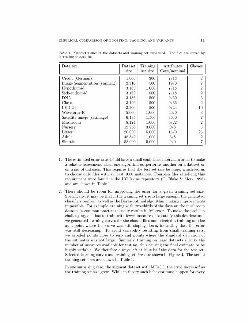
Table 1. Characteristics of the datasets and training set sizes used. The files are sorted byincreasing dataset size
Data set Dataset Training Attributes Classessize set size Cont/nominal
Credit (German) 1,000 300 7/13 2Image Segmentation (segment) 2,310 500 19/0 7Hypothyroid 3,163 1,000 7/18 2Sick-euthyroid 3,163 800 7/18 2DNA 3,186 500 0/60 3Chess 3,196 500 0/36 2LED-24 3,200 500 0/24 10Waveform-40 5,000 1,000 40/0 3Satellite image (satimage) 6,435 1,500 36/0 7Mushroom 8,124 1,000 0/22 2Nursery 12,960 3,000 0/8 5Letter 20,000 5,000 16/0 26Adult 48,842 11,000 6/8 2Shuttle 58,000 5,000 9/0 7
1. The estimated error rate should have a small confidence interval in order to makea reliable assessment when one algorithm outperforms another on a dataset oron a set of datasets. This requires that the test set size be large, which led usto choose only files with at least 1000 instances. Fourteen files satisfying thisrequirement were found in the UC Irvine repository (C. Blake & Merz 1998)and are shown in Table 1.
2. There should be room for improving the error for a given training set size.Specifically, it may be that if the training set size is large enough, the generatedclassifiers perform as well as the Bayes-optimal algorithm, making improvementsimpossible. For example, training with two-thirds of the data on the mushroomdataset (a common practice) usually results in 0% error. To make the problemchallenging, one has to train with fewer instances. To satisfy this desideratum,we generated learning curves for the chosen files and selected a training set sizeat a point where the curve was still sloping down, indicating that the errorwas still decreasing. To avoid variability resulting from small training sets,we avoided points close to zero and points where the standard deviation ofthe estimates was not large. Similarly, training on large datasets shrinks thenumber of instances available for testing, thus causing the final estimate to behighly variable. We therefore always left at least half the data for the test set.Selected learning curves and training set sizes are shown in Figure 4. The actualtraining set sizes are shown in Table 1.
In one surprising case, the segment dataset with MC4(1), the error increased asthe training set size grew. While in theory such behavior must happen for every

12 ERIC BAUER AND RON KOHAVI
induction algorithm (Wolpert 1994, Schaffer 1994), this is the first time we haveseen it in a real dataset. Further investigation revealed that in this problemall seven classes are equiprobable, i.e., the dataset was stratified. A strongmajority in the training set implies a non-majority in the test set, resultingin poor performance. A stratified holdout might be more appropriate in suchcases, mimicking the original sampling methodology (Kohavi 1995b). For ourexperiments, only relative performance mattered, so we did not specificallystratify the holdout samples.
3. The voting algorithms should combine relatively few sub-classifiers. Similar inspirit to the use of the learning curves, it is possible that two voting algorithmswill reach the same asymptotic error rate but that one will reach it using fewersub-classifiers. If both are allowed to vote a thousand classifiers as was donein Schapire et al. (1997), “slower” variants that need more sub-classifiers tovote may seem just as good. Quinlan (1996) used only 10 replicates, whileBreiman (1996b) used 50 replicates and Freund & Schapire (1996) used 100.Based on these numbers and graphs of boosting error rates versus the numberof trials/sub-classifiers, we chose to vote 25 sub-classifiers throughout the paper.
This decision on limiting the number of sub-classifiers is also important forpractical applications of voting methods. To be competitive, it is importantthat the algorithms run in reasonable time. Based on our experience, we believethat an order of magnitude difference is reasonable but that two or three ordersof magnitude is unreasonable in many practical applications; for example, arelatively large run of the base inducer (e.g., MC4) that takes an hour todaywill take 4–40 days if the voted version runs 100–1000 times slower because thatmany trials are used.
6.2. Sanity Check for Correctness
As mentioned earlier, our implementations of the MC4 and Naive-Bayes inducerssupport instance weights within the algorithms themselves. This results in a closercorrespondence to the theory defining voting classifiers. To ensure that our im-plementation is correct and that the algorithmic changes did not cause significantdivergence from past experiments, we repeated the experiments of Breiman (1996b)and Quinlan (1996) using our implementation of voting algorithms.
The results showed similar improvements to those described previously. For ex-ample, Breiman’s results show CART with Bagging improving average error overnine datasets from 12.76% to 9.69%, a relative gain of 24%, whereas our Bagging ofMC4 improved the average error over the same datasets from 12.91% to 9.91%, arelative gain of 23%. Likewise, Quinlan showed how boosting C4.5 over 22 datasets(that we could find for our replication experiment) produced a gain in accuracy of19%; our experiments with boosting MC4 also show a 19% gain for these datasets.This confirmed the correctness of our methods.
EMPIRICAL COMPARISON OF BOOSTING, BAGGING, AND VARIANTS 13
6.3. Runs and Measurements
The runs we used to estimate error rates fell into two categories: bias-varianceand repeated holdout. The bias-variance details were given in Section 5 and werethe preferred method throughout this work, since they provided an estimate of theerror for the given holdout size and gave its decomposition into bias and variance.
We ran holdouts, repeated three times with a different seed each time, in twocases. First, we used holdout when generating error rates for different numbers ofvoting trials. In this case the bias-variance decomposition does not vary much acrosstime, and the time penalty for performing this experiment with the bias-variancedecomposition as well as with a varying number of trials was too high. The seconduse was for measuring mean-squared errors. The bias-variance decomposition forclassification does not extend to mean-squared errors, because labels in classificationtasks have no associated probabilities.
The estimated error rates for the two experimental methods differed in somecases, especially for the smaller datasets. However, the difference in error ratesbetween the different induction algorithms tested under both methods was verysimilar. Thus, while the absolute errors presented in this paper may have largevariance in some cases, the differences in errors are very accurate because all thealgorithms were trained and tested on exactly the same training and test sets.
When we compare algorithms below, we summarize information in two ways.First, we give the decrease or increase in average (absolute) error averaged overall our datasets, assuming they represent a reasonable “real-world” distributionof datasets. Second, we give the average relative error reduction. For twoalgorithms A and B with errors εA and εB, the decrease in relative error betweenA and B is (εA−εB)/εA. For example, if algorithm B has a 1% error and algorithmA had a 2% error, the absolute error reduction is only 1%, but the relative errorreduction is 50%. The average relative error is the average (over all our datasets)of the relative error between the pair of algorithms compared. Relative error hasbeen used in Breiman (1996b) and in Quinlan (1996), under the names “ratio” and“average ratio” respectively.
Note that average relative error reduction is different from the relative reductionin average error; the computation for the latter involves averaging the errors firstand then computing the ratio. The relative reduction in average error can becomputed from the two error averages we supply, so we have not explicitly statedit in the paper to avoid an overload of numbers.
The computations of error, relative errors, and their averages were done in highprecision by our program. However, for presentation purposes, we show only onedigit after the decimal point, so some numbers may not add up exactly (e.g., thebias and variance may be off by 0.1% from the error).
7. The Bagging Algorithm and Variants
We begin with a comparison of MC4 and Naive-Bayes with and without Bagging.We then proceed to variants of Bagging that include pruning versus no pruning
14 ERIC BAUER AND RON KOHAVI
german0.00
5.00
10.00
15.00
20.00
25.00
30.00
segment0.00
2.00
4.00
6.00
8.00
hypothyroid0.00
0.20
0.40
0.60
0.80
1.00
1.20
1.40
sick-euthyroid0.00
0.50
1.00
1.50
2.00
2.50
3.00
DNA-nominal0.00
2.00
4.00
6.00
8.00
10.00
12.00
14.00
chess0.00
0.50
1.00
1.50
2.00
2.50
3.00
led240.00
5.00
10.00
15.00
20.00
25.00
30.00
35.00
waveform-400.00
5.00
10.00
15.00
20.00
25.00
30.00
satimage0.00
5.00
10.00
15.00
20.00
mushroom0.00
0.10
0.20
0.30
0.40
0.50
nursery0.00
1.00
2.00
3.00
4.00
5.00
6.00
7.00
letter0.00
5.00
10.00
15.00
20.00
25.00
adult0.00
5.00
10.00
15.00
20.00
shuttle0.00
0.05
0.10
0.15
0.20
0.25
10.00
5.00
10.00
15.00MC4
bagged MC4
bagged MC4 without pruning with prob. estimates
bagged MC4 without pruning with prob. estimates and backfitting
Bias is below variance
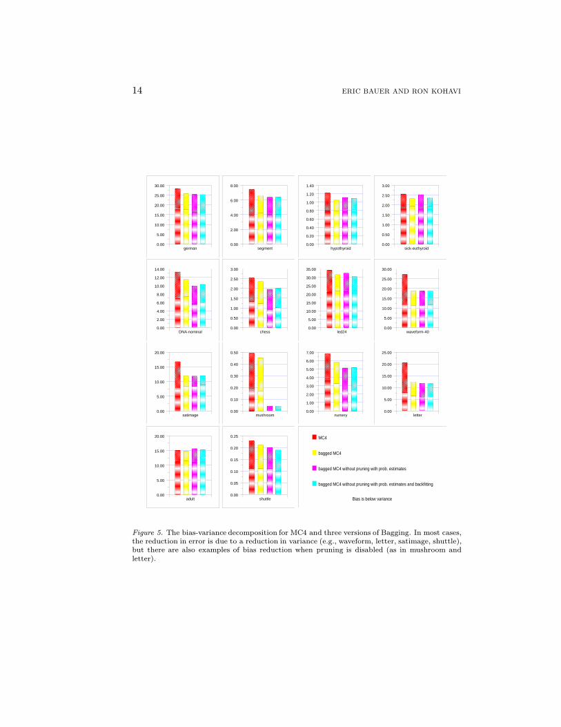
Figure 5. The bias-variance decomposition for MC4 and three versions of Bagging. In most cases,the reduction in error is due to a reduction in variance (e.g., waveform, letter, satimage, shuttle),but there are also examples of bias reduction when pruning is disabled (as in mushroom andletter).

EMPIRICAL COMPARISON OF BOOSTING, BAGGING, AND VARIANTS 15
Algorithms
Err
or (
%)
0.00
2.00
4.00
6.00
8.00
10.00
12.00
14.00
MC4
Bagged MC4
Above without pruning
Above with p-Bagging
Above with backfitting
Bias is below variance
Algorithms
Err
or (
%)
0.00
5.00
10.00
15.00
20.00
25.00
30.00
35.00
MC4(1)-disc
Bagged MC4(1)-disc
p-Bagged MC4(1)-disc
Bias is below variance
Algorithms
Err
or (
%)
0.00
2.00
4.00
6.00
8.00
10.00
12.00
14.00
Naive-Bayes
Bagged Naive-Bayes
p-Bagged Naive-Bayes
Bias is below variance
Figure 6. The average bias and variance over all datasets for several variants of Bagging withthree induction algorithms. MC4 and MC4(1)-disc improve significantly due to variance reduction;Naive-Bayes is a stable inducer and improves very little (as expected).
and classifications versus probabilistic estimates (scoring). Figure 5 shows the bias-variance decomposition for all datasets using MC4 with three versions of Baggingexplained below. Figure 6 shows the average bias and variance over all the datasetsand for MC4, Naive-Bayes, and MC4(1)-disc.
7.1. Bagging: Error, Bias, and Variance
In the decomposition of error into bias and variance, applying Bagging to MC4caused the average absolute error to decrease from 12.6% to 10.4%, and the averagerelative error reduction was 14.5%.
The important observations are:
1. Bagging is uniformly better for all datasets. In no case did it increase the error.
2. Waveform-40, satimage, and letter’s error rate decreased dramatically, withrelative reductions of 31%, 29%, and 40%. For the other datasets, the relativeerror reduction was less than 15%.
3. The average tree size (number of nodes) for the trees generated by Baggingwith MC4 was slightly larger than the trees generated by MC4 alone: 240nodes versus 198 nodes. The average tree size (averaged over the replicates fora dataset) was larger eight times, of which five averages were larger by morethan 10%. In comparison, only six trees generated by MC4 alone were largerthan Bagging, of which only three were larger by more than 10%. For the adultdataset, the average tree size from the Bagged MC4 was 1510 nodes comparedto 776 nodes for MC4. This is above and beyond the fact that the Baggedclassifier contains 25 such trees.
We hypothesize that the larger tree sizes might be due to the fact that originalinstances are replicated in Bagging samples, thus implying a stronger patternand reducing the amount of pruning. This hypothesis and related hypothesesare tested in Section 7.2.

16 ERIC BAUER AND RON KOHAVI
4. The bias-variance decomposition shows that error reduction is almost com-pletely due to variance reduction: the average variance decreased from 5.7% to3.5% with a matching 29% relative reduction. The average bias reduced from6.9% to 6.8% with an average relative error reduction of 2%.
The Bagging algorithm with MC4(1) reduced the error from 38.2% to 37.3%with a small average reduction in relative error of 2%. The bias decreased from27.6% to 26.9% and the variance decreased from 10.6% to 10.4%. We attributethe reduction in bias to the slightly stronger classifier that is formed with Bagging.The low reduction in variance is expected, since shallow trees with a single rootsplit are relatively stable.
The Bagging algorithm with MC4(1)-disc reduced the error from 33.0% to 31.5%,an average relative error reduction of 4%. The bias increased from 24.4% to 25.0%(mostly due to to waveform, where bias increased by 5.6% absolute error) and thevariance decreased from 8.6% to 6.5%. We hypothesize that the bias increase is dueto an inferior discretization when Bagging is used, since the discretization does nothave access to the full training set, but only to a sample containing about 63.2%unique instances.
The Bagging algorithm with Naive-Bayes reduced the average absolute error from13.6% to 13.2%, and the average relative error reduction was 3%.
7.2. Pruning
Two effects described in the previous section warrant further investigation: thelarger average size for trees generated by Bagging and the slight reduction in biasfor Bagging. This section deals only with unbounded-depth decision trees built byMC4 not MC4(1) or MC4(1)-disc.
We hypothesized that larger trees were generated by MC4 when using bootstrapreplicates because the pruning algorithm pruned less, not because larger trees wereinitially grown. To verify this hypothesis, we disabled the pruning algorithm andreran the experiments. The MC4 default—like C4.5—grows the trees until nodesare pure or until a split cannot be found where two children each contain at leasttwo instances.
The unpruned trees for MC4 had an average size of 667 and the unpruned treesfor Bagged MC4 trees had an average size of 496—25% smaller. Moreover, theaveraged size for trees generated by MC4 on the bootstrap samples for a givendataset was always smaller than the corresponding size of the trees generated byMC4 alone. We postulate that this effect is due to the smaller effective size oftraining sets under bagging, which contain only about 63.2% unique instances fromthe original training set. Oates & Jensen (1997) have shown that there is a closecorrelation between the training set size and the tree complexity for the reducederror pruning algorithm used in C4.5 and MC4.
The trees generated from the bootstrap samples were initially grown to be smallerthan the corresponding MC4 trees, yet they were larger after pruning was invoked.The experiment confirms our hypothesis that the structure of the bootstrap repli-cates inhibits reduced-error pruning. We believe the reason for this inhibition is

EMPIRICAL COMPARISON OF BOOSTING, BAGGING, AND VARIANTS 17
that instances are duplicated in the bootstrap sample, reinforcing patterns thatmight otherwise be pruned as noise.
The non-pruned trees generated by Bagging had significantly smaller bias thantheir pruned counterparts: 6.6% versus 6.9%, or a 14% average relative error reduc-tion. This observation strengthens the hypothesis that the reduced bias in Baggingis due to larger trees, which is expected: pruning increased the bias but decreasedthe variance. Indeed, the non-Bagged unpruned trees have a similar bias of 6.6%(down from 6.9%).
However, while bias is reduced for non-pruned trees (for both Bagging with MC4and MC4 alone), variance for trees generated by MC4 grew dramatically: from5.7% to 7.3%, thus increasing the overall error from 12.6% to 14.0%. The variancefor Bagging grows less, from 3.5% to 3.9%, and the overall error remains the sameat 10.4%. The average relative error decreased by 7%, mostly due to a decrease inthe absolute error of mushroom from 0.45% to 0.04%—a 91% decrease (note howthis impressive decrease corresponds to a small change in absolute error).
7.3. Using Probabilistic Estimates
Standard Bagging uses only the predicted classes, i.e., the combined classifier pre-dicts the class most frequently predicted by the sub-classifiers built from the boot-strap samples. Both MC4 and Naive-Bayes can make probabilistic predictions,and we hypothesized that this information would further reduce the error. Ouralgorithm for combining probabilistic predictions is straightforward. Every sub-classifier returns a probability distribution for the classes. The probabilistic bag-ging algorithm (p-Bagging) uniformly averages the probability for each class (overall sub-classifiers) and predicts the class with the highest probability.
In the case of decision trees, we hypothesized that unpruned trees would givemore accurate probability distributions in conjunction with voting methods for thefollowing reason: a node that has a 70%/30% class distribution can have childrenthat are 100%/0% and 60%/40%, yet the standard pruning algorithms will alwaysprune the children because the two children predict the same class. However, ifprobability estimates are needed, the two children may be much more accurate,since the child having 100%/0% is identifying a perfect cluster (at least in thetraining set). For single trees, the variance penalty incurred by using estimates fromnodes with a small number of instances may be large and pruning can help (Pazzani,Merz, Murphy, Ali, Hume & Brunk 1994); however, voting methods reduce thevariance by voting multiple classifiers, and the bias introduced by pruning may bea limiting factor.
To test our hypothesis that probabilistic estimates can help, we reran the bias-variance experiments using p-Bagging with both Naive-Bayes and MC4 with prun-ing disabled.
The average error for MC4 decreased from 10.4% to 10.2% and the average relativeerror decreased by 2%. This decrease was due to both bias and variance reduction.The bias reduced from 6.5% to 6.4% with an average relative decrease of 2%. Thevariance decreased from 3.9% to 3.8% with an average relative decrease of 4%.
18 ERIC BAUER AND RON KOHAVI
The average error for MC4(1) decreased significantly from 37.3% to 34.4%, withan average relative error reduction of 4%. The reduction in bias was from 26.9% to24.9% and the reduction in variance was from 10.4% to 9.5%
The average error for MC4(1)-disc decreased from 33.0% to 28.9%, an averagerelative reduction of 8%. The bias decreased from 25.0% to 23.0%, an averagerelative reduction of 3% (compared to an increase in bias for the non-probabilisticversion). The variance decreased from 8.6% to 5.9%, an average relative errorreduction of 17%.
The average error for Naive-Bayes decreased from 14.22% to 14.15% and the av-erage relative error decreased 0.4%. The bias decreased from 11.45% to 11.43%with zero relative bias reduction and the variance decreased from 2.77% to 2.73%with a 2% relative variance reduction. These results for Naive-Bayes are insignifi-cant. As is expected, the error incurred by Naive-Bayes is mostly due to the biasterm. The probability estimates generated are usually extreme because the condi-tional independence assumption is not true in many cases, causing a single factorto affect several attributes whose probabilities are multiplied assuming they areconditionally independent given the label (Friedman 1997).
To summarize, we have seen error reductions for the family of decision-tree algo-rithms when probabilistic estimates were used. The error reductions were larger forthe one level decision trees. This reduction was due to a decrease in both bias andvariance. Naive-Bayes was mostly unaffected by the use of probabilistic estimates.
7.4. Mean-Squared Errors
In many practical applications it is important not only to classify correctly, but alsoto give a probability distribution on the classes. A common measure of error on sucha task is mean-squared error (MSE), or the squared difference of the probabilityfor the class and the probability predicted for it. Since the test set assigns a labelwithout a probability, we measure the MSE as (1 − P(Ci(x)))2, or one minus theprobability assigned to the correct label. The average MSE is the mean-squarederror averaged over the entire test set. If the classifier assigns a probability of oneto the correct label, then the penalty is zero; otherwise, the penalty is positive andgrows with the square of the distance from one.
A classifier that makes a single prediction is viewed as assigning a probability ofone to the predicted class and zero to the other classes. Under those conditions, theaverage MSE is the same as the classification error. Note, however, that our resultsare slightly different (less than 0.1% error for averages) because five times holdoutwas used for these runs as compared to 3 times 10 holdout for the bias-varianceruns above, which cannot compute the MSE.
To estimate whether p-Bagging is really better at estimating probabilities, we raneach inducer on each datafile five times using a holdout sample of the same effectivesize as was used for the bias-variance experiments. For MC4, the average MSEdecreased from 10.4% for Bagging with no pruning (same as the classification errorabove) to 7.5% for p-Bagging with probability estimates—a 21% average relativereduction. If MC4 itself is run in probability estimate mode using frequency counts,
EMPIRICAL COMPARISON OF BOOSTING, BAGGING, AND VARIANTS 19
its average MSE is 10.7%; if we apply an m-estimate Laplace correction to the leavesas described in Kohavi, Becker & Sommerfield (1997), the average MSE decreasedto 10.0%, but p-Bagging still significantly outperformed this method, reducing theaverage relative MSE by 21%.
For Naive-Bayes, the average MSE went down from 13.1% to 9.8%, an averagerelative reduction of 24%. When Naive-Bayes was run in probability estimate mode,the MSE was 10.5%, and there was no average relative MSE difference.
For MC4(1)-disc, the average MSE went down from 31.1% to 18.4%, a 34% de-crease in average relative MSE. However, running MC4(1)-disc in probability esti-mate mode gave an average MSE of 19.5%, so most of the benefit came not fromBagging but from using probability estimates. Indeed, the children of the rootusually tend to give fairly accurate probability estimates (albeit based on a singleattribute).
From the above results, we can see that applying m-estimate Laplace correctionsduring classification in MC4 significantly reduces the average MSE and that p-Bagging reduces it significantly more. For Naive-Bayes, the main improvementresults from switching to probabilities from classification, but there is a small benefitto using p-Bagging.
7.5. Wagging and Backfitting Data
An interesting variant of Bagging that we tried is called Wagging (WeightAggregation). This method seeks to repeatedly perturb the training set as inBagging, but instead of sampling from it, Wagging adds Gaussian noise to eachweight with mean zero and a given standard deviation (e.g., 2). For each trial,we start with uniformly weighted instances, add noise to the weights, and inducea classifier. The method has the nice property that one can trade off bias andvariance: by increasing the standard deviation of the noise we introduce, more in-stances will have their weight decrease to zero and disappear, thus increasing biasand reducing variance. Experiments showed that with a standard deviation of 2-3,the method finishes head-to-head with the best variant of Bagging used above, i.e.,the error of Bagged MC4 without pruning and with scoring was 10.21% and theerrors for Wagging with 2, 2.5, and 3 were 10.19%, 10.16%, and 10.12%. Thesedifferences are not significant. Results for Naive-Bayes were similar.
A more successful variant that we tried for MC4 uses a method called backfittingdescribed below. Bagging creates classifiers from about 63.2% unique instances inthe training set. To improve the probability estimates at the leaves of the decisiontree, the algorithm does a second “backfit” pass after sub-classifier construction,feeding the original training set into the decision tree without changing its structure.The estimates at the leaves are now expected to be more accurate as they are basedon more data.
Indeed, a bias-variance run shows that the error for Bagging MC4 without pruningand with scoring reduces the error from 10.4% to 10.1%; the average relative errordecreased by 3%. The bias and variance decomposition shows that the bias is aboutthe same: 6.7% with backfitting and 6.6% without backfitting, but the variance is
20 ERIC BAUER AND RON KOHAVI
0
2
4
6
8
10
12
14
16
18
20
0 5 10 15 20 25
Err
or (
%)
Number of trials
satimage
Test error of bagged MC4Train error of bagged MC4
Test error of Bagged MC4 without pruning, with prob. estimates and backfittingTrain error of Bagged MC4 without pruning, with prob. estimates and backfitting
0
0.5
1
1.5
2
2.5
3
3.5
0 5 10 15 20 25
Err
or (
%)
Number of trials
chess
Test error of bagged MC4Train error of bagged MC4
Test error of Bagged MC4 without pruning, with prob. estimates and backfittingTrain error of Bagged MC4 without pruning, with prob. estimates and backfitting
0
2
4
6
8
10
12
14
16
18
0 5 10 15 20 25
Err
or (
%)
Number of trials
DNA-nominal
Test error of bagged MC4Train error of bagged MC4
Test error of Bagged MC4 without pruning, with prob. estimates and backfittingTrain error of Bagged MC4 without pruning, with prob. estimates and backfitting
0
1
2
3
4
5
6
7
8
9
0 5 10 15 20 25
Err
or (
%)
Number of trials
nursery
Test error of bagged MC4Train error of bagged MC4
Test error of Bagged MC4 without pruning, with prob. estimates and backfittingTrain error of Bagged MC4 without pruning, with prob. estimates and backfitting
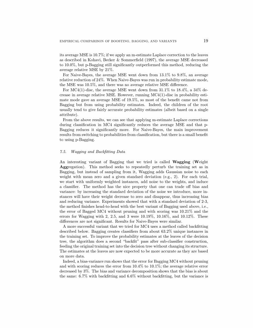
Figure 7. Bagging graphs for selected datasets showing different behaviors of MC4 and the originalBagging versus the backfit-p-Bagging. The graphs show the test set and training set errors asthe number of bootstrap samples (replicates) increases. Each point shows error performance forthe set of classifiers created by the bagging algorithm so far, averaged of three 25-trial runs.Satimage represents the largest family where both versions track each other closely and wheremost of the improvement happens in the first five to ten trials. Chess represents a case wherebackfit-p-Bagging is initially better but flattens out and Bagging matches it in later trials. DNA-nominal and nursery are examples where backfit-p-Bagging is superior throughout and seems tokeep its advantage. Note how low the training set errors were, implying that the decision treesare overfitting.
reduced from 3.9% to 3.4% with an average relative variance decrease of 11%. Infact, the variance for all files either remained the same or was reduced!
Figure 7 shows graphs of how error changes over trials for selected datasets thatrepresent the different behaviors we have seen for the initial version of Bagging andthe final backfitting version for MC4. The graphs show both test set and trainingset error as the number of bootstrap samples increases. In no case did Baggingsignificantly outperform backfit-p-Bagging.
7.6. Conclusions on Bagging
We have shown a series of variants for Bagging, each of which improves performanceslightly over its predecessor for the MC4 algorithm. The variants were: disablingpruning, using average probability estimates (scores), and backfitting. The errordecreased from 10.34% for the original Bagging algorithm to 10.1% for the final
EMPIRICAL COMPARISON OF BOOSTING, BAGGING, AND VARIANTS 21
version (compared to 12.6% for MC4). The average relative decrease in error was10%, although most of it was due to mushroom, which reduced from 0.45% to 0.04%(a 91% relative decrease). Even excluding mushroom, the average relative decreasein error was 4%, which is impressive for an algorithm that performs well initially.
For MC4, the original Bagging algorithm achieves most of its benefit by reducingvariance from 5.7% to 3.5%. Our final version decreased the variance slightly more(to 3.4%) and decreased the bias from 6.8% to 6.6%.
Bagging also reduces the error for MC4(1), which was somewhat surprising to usinitially, as we did not expect the variance of one-level trees to be large and thoughtthat Bagging would have no effect. However, the error did decrease from 38.2%to 34.4%, and analyzing the results showed that this change is due mostly to biasreduction of 2.6% and a variance reduction of 1.1%. A similar effect was true forMC4(1)-disc: the error reduced from 33.0% to 28.9%.
While Naive-Bayes has been successful on many datasets (Domingos & Pazzani1997, Friedman 1997, Langley & Sage 1997, Kohavi 1995b) (although usually cou-pled with feature selection which we have not included in this study), it starts outinferior to MC4 in our experiments (13.6% error for Naive-Bayes versus 12.6% er-ror for MC4) and the difference only grows. The MC4 error decreased to 10.1%,while Naive-Bayes went down to only 13.2%. Naive-Bayes is an extremely stablealgorithm, and Bagging is mostly a variance reduction technique. Specifically, theaverage variance for Naive-Bayes is 2.8%, which Bagging with probability estimatesdecreased to 2.5%. The average bias, however, is 10.8%, and Bagging reduces thatto only 10.6%.
The mean-squared errors generated by p-Bagging were significantly smaller thanthe non-Bagged variants for MC4, MC4(1), and MC4(1)-disc. We are not aware ofanyone who reported any mean-squared errors results for voting algorithms in thepast. Good probability estimates are crucial for applications when loss matricesare used (Bernardo & Smith 1993), and the significant differences indicate thatp-Bagging is a very promising approach.
8. Boosting Algorithms: AdaBoost and Arc-x4
We now discuss boosting algorithms. First, we explore practical considerations forboosting algorithm implementation, specifically numerical instabilities and under-flows. We then show a detailed example of a boosting run and emphasize under-flow problems we experienced. Finally, we show results from experiments usingAdaBoost and Arc-x4 and describe our conclusions.
8.1. Numerical Instabilities and a Detailed Boosting Example
Before we detail the results of the experiments, we would like to step through adetailed example of an AdaBoost run for two reasons: first, to get a better under-standing of the process, and second, to highlight the important issue of numericalinstabilities and underflows that is rarely discussed yet common in boosting al-gorithms. We believe that many authors have either faced these problems and

22 ERIC BAUER AND RON KOHAVI
corrected them or do not even know that they exist, as the following exampleshows.
Example: Domingos & Pazzani (1997) reported very poor accuracy of 24.1% (er-ror of 75.9%) on the Sonar dataset with the Naive-Bayes induction algorithm, whichotherwise performed very well. Since this is a two-class problem, predicting major-ity would have done much better. Kohavi, Becker & Sommerfield (1997) reportedan accuracy of 74.5% (error of 25.5%) on the same problem with a very similar algo-rithm. Further investigation of the discrepancy by Domingos and Kohavi revealedthat Domingos’ Naive-Bayes algorithm did not normalize the probabilities afterevery attribute. Because there are 60 attributes, the multiplication underflowed,creating many zero probabilities.
Numerical instabilities are a problem related to underflows. In several cases inthe past, we have observed problems with entropy computations that yield smallnegative results (on the order of −10−13 for 64-bit double-precision computations).The problem is exacerbated when a sample has both small- and large-weight in-stances (as occurs during boosting). When instances have very small weights, thetotal weight of the training set can vary depending on the summation order (e.g.,shuffling and summing may result in a slightly different sum). From the standpointof numerical analysis, sums should be done from the smallest to the largest numbersto reduce instability, but this imposes severe burdens (in terms of programming andrunning-time) on standard computations.
In MLC++, we defined the natural weight of an instance to be one, so that fora sample with unweighted instances, the total weight of the sample is equal tothe number of instances. The normalization operations required in boosting weremodified accordingly. To mitigate numerical instability problems, instances withweights of less than 10−6 are automatically removed.
In our initial implementation of boosting, we had several cases where many in-stances were removed due to underflows as the described below. We explore anexample boosting run both to show the underflow problem and to help the readerdevelop a feel for how the boosting process functions.
Example: A training set of size 5,000 was used with the shuttle dataset. The MC4algorithm already has relatively small test set error (measured on the remaining53,000 instances) of 0.38%. The following is a description of progress by trials, alsoshown in Figure 8.
1. The training set error for the first (uniformly weighted, top-left in Figure 8)boosting trial is 0.1%, or five misclassified instances. The update rule in Equa-tion 1 on page 6 shows that these five instances will now be re-weighted froma weight of one to a weight of 500 (the update factor is 1/(2 · 0.1%)), while thecorrectly classified instances will have their weight halved (1/(2(1 − 0.1%)) =1/1.998) to a weight of about 0.5. As with regular MC4, the test set error forthe first classifier is 0.38%.

EMPIRICAL COMPARISON OF BOOSTING, BAGGING, AND VARIANTS 23
Figure 8. The shuttle dataset projected on the three most discriminatory axes. Color/shadingdenotes the class of instances and the cube sizes correspond to the instance weights. Each pictureshows one AdaBoost trial, where progression is from the top left to top right, then middle left,etc.
24 ERIC BAUER AND RON KOHAVI
2. On the second trial, the classifier trained on the weighted sample makes amistake on a single instance that was not previously misclassified (shown intop-right figure as red, very close to the previous large red instance). Thetraining set error is hence 0.5/5000 = 0.01%, and that single instance willweigh 2500—exactly half of the total weight of the sample! The weight of thecorrectly classified instances will be approximately halved, changing the weightsfor the four mistaken instances from trial one to around 250 and the weightsfor the rest of the instances to about 0.25. The test set error for this classifieralone is 0.19%
3. On the third trial (middle-left in Figure 8), the classifier makes five mistakesagain, all on instances correctly classified in previous trials. The training seterror is hence about 5 · 0.25/5000 = 0.025%. The weight of the instance in-correctly classified in trial two will be approximately halved to about 1250 andthe five incorrectly classified instances will now occupy half the weight—exactly500 each. All the other instances will weigh about 0.125. The test set error forthis classifier alone is 0.21%
4. On the fourth trial (middle-right in Figure 8), the classifier makes 12 mistakeson the training set. The training set error is 0.03% and the test set error is0.45%.
5. On the fifth trial (lower-left in Figure 8), the classifier makes one mistake on aninstance with weight 0.063. The training set error is therefore 0.0012%.
In our original implementation, we used the update rule recommended in thealgorithm shown in the AdaBoost algorithm in Figure 2. Because the error is sosmall, β is 1.25 ·10−5; multiplying the weights by this β (prior to normalization)caused them to underflow below the minimum allowed weight of 10−6. Almostall instances were then removed, causing the sixth trial to have zero trainingset error but 60.86% test set error.
In our newer implementation, which we use in the rest of the paper, the updaterule in Equation 1 on page 6 is used, which suffers less from underflow problems.
6. On the sixth trial (lower-right in Figure 8), the classifier makes no mistakes andhas a test set error of 0.08% (compared to 0.38% for the original decision-treeclassifier). The process then stops. Because this classifier has zero training seterror, it gets “infinite voting” power. The final test set error for the AdaBoostalgorithm is 0.08%.
The example above is special because the training set error for a single classifierwas zero for one of the boosting trials. In some sense, this is a very interestingresult because a single decision classifier was built that had a test set error thatwas relatively better than the original decision tree by 79%. This is really not anensemble but a single classifier!
Using the update rule that avoids the normalization step mainly circumvents theissue of underflow early in the process, but underflows still happen. If the error isclose to zero, instances that are correctly classified in k trials are reduced by a factor
EMPIRICAL COMPARISON OF BOOSTING, BAGGING, AND VARIANTS 25
of about 2k. For our experiments with 25 trials, weights can be reduced to about3 · 10−8, which is well below our minimum threshold. For the rest of the paper, thealgorithm used sets instances with weights falling below the minimum weight tohave the minimum weight. Because most runs have significantly larger error thanin the above example (especially after a few boosting trials), the underflow issue isnot severe.
Recent boosting implementations by Freund, Schapire, and Singer maintain thelog of the weights and modify the definition of β so that a small value (0.5 dividedby the number of training examples) is added to the numerator and denominator(personal communication with Schapire, 1997). It seems that the issue deservescareful attention and that boosting experiments with many trials (e.g., 1000 as inSchapire et al. (1997)) require addressing the issue carefully.
8.2. AdaBoost: Error, Bias, and Variance
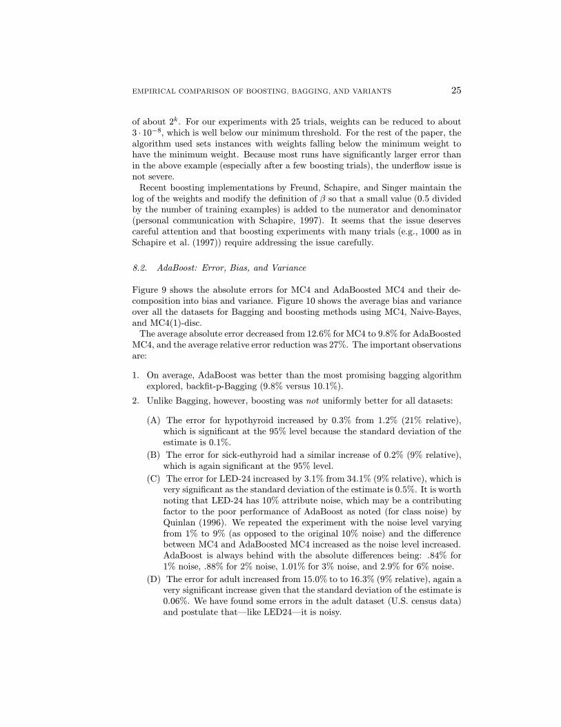
Figure 9 shows the absolute errors for MC4 and AdaBoosted MC4 and their de-composition into bias and variance. Figure 10 shows the average bias and varianceover all the datasets for Bagging and boosting methods using MC4, Naive-Bayes,and MC4(1)-disc.
The average absolute error decreased from 12.6% for MC4 to 9.8% for AdaBoostedMC4, and the average relative error reduction was 27%. The important observationsare:
1. On average, AdaBoost was better than the most promising bagging algorithmexplored, backfit-p-Bagging (9.8% versus 10.1%).
2. Unlike Bagging, however, boosting was not uniformly better for all datasets:
(A) The error for hypothyroid increased by 0.3% from 1.2% (21% relative),which is significant at the 95% level because the standard deviation of theestimate is 0.1%.
(B) The error for sick-euthyroid had a similar increase of 0.2% (9% relative),which is again significant at the 95% level.
(C) The error for LED-24 increased by 3.1% from 34.1% (9% relative), which isvery significant as the standard deviation of the estimate is 0.5%. It is worthnoting that LED-24 has 10% attribute noise, which may be a contributingfactor to the poor performance of AdaBoost as noted (for class noise) byQuinlan (1996). We repeated the experiment with the noise level varyingfrom 1% to 9% (as opposed to the original 10% noise) and the differencebetween MC4 and AdaBoosted MC4 increased as the noise level increased.AdaBoost is always behind with the absolute differences being: .84% for1% noise, .88% for 2% noise, 1.01% for 3% noise, and 2.9% for 6% noise.
(D) The error for adult increased from 15.0% to to 16.3% (9% relative), again avery significant increase given that the standard deviation of the estimate is0.06%. We have found some errors in the adult dataset (U.S. census data)and postulate that—like LED24—it is noisy.
26 ERIC BAUER AND RON KOHAVI
german0.00
5.00
10.00
15.00
20.00
25.00
30.00
segment0.00
2.00
4.00
6.00
8.00
hypothyroid0.00
0.50
1.00
1.50
2.00
sick-euthyroid0.00
0.50
1.00
1.50
2.00
2.50
3.00
3.50
DNA-nominal0.00
2.00
4.00
6.00
8.00
10.00
12.00
14.00
chess0.00
0.50
1.00
1.50
2.00
2.50
3.00
led240.00
10.00
20.00
30.00
40.00
waveform-400.00
5.00
10.00
15.00
20.00
25.00
30.00
satimage0.00
5.00
10.00
15.00
20.00
mushroom0.00
0.10
0.20
0.30
0.40
0.50
nursery0.00
1.00
2.00
3.00
4.00
5.00
6.00
7.00
letter0.00
5.00
10.00
15.00
20.00
25.00
adult0.00
5.00
10.00
15.00
20.00
shuttle0.00
0.05
0.10
0.15
0.20
0.25 MC4
bagged MC4 without pruning with prob. estimates and backfitting
boosted MC4 using Arc-x4-resample
boosted MC4 using AdaBoost
Bias is below variance
Figure 9. The bias and variance decomposition for MC4, backfit-p-Bagging, Arc-x4-resample,and AdaBoost. The boosting methods (Arc-x4 and AdaBoost) are able to reduce the bias overBagging in some cases (e.g., DNA, chess, nursery, letter, shuttle). However, they also increase thevariance (e.g., hypothyroid, sick-euthyroid, LED-24, mushroom, and adult).
EMPIRICAL COMPARISON OF BOOSTING, BAGGING, AND VARIANTS 27
Algorithms
Err
or (
%)
0.00
2.00
4.00
6.00
8.00
10.00
12.00
14.00
MC4
Backfitted p-Bagged MC4
Boosted MC4 with Arc-x4
Boosted MC4 with AdaBoost
Bias is below variance
Algorithms
Err
or (
%)
0.00
5.00
10.00
15.00
20.00
25.00
30.00
35.00
MC4(1)-disc
p-Bagged MC4(1)-disc
Boosted MC(1)-disc with Arc-x4
Boosted MC(1)-disc with AdaBoost
Bias is below variance
Algorithms
Err
or (
%)
0.00
2.00
4.00
6.00
8.00
10.00
12.00
14.00
Naive-Bayes
p-Bagged Naive-Bayes
Boosted Naive-Bayes with Arc-x4
Boosted Naive-Bayes with AdaBoost
Bias is below variance
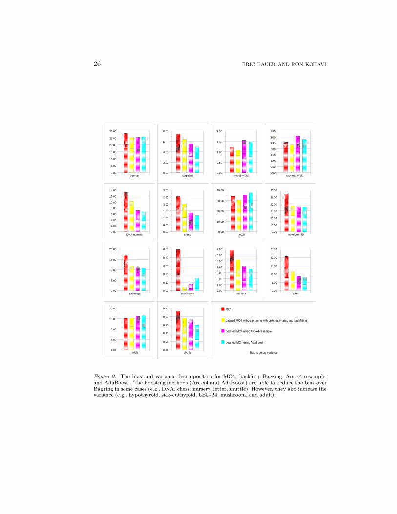
Figure 10. The average bias and variance over all datasets for backfit-p-Bagging, two boostingvariants and three inductions algorithms. Both boosting algorithms outperform backfit-p-Baggingalthough the differences are more noticeable with Naive-Bayes and MC4(1)-disc. Somewhat sur-prisingly, Arc-x4-resample is superior to AdaBoost for Naive-Bayes and MC4(1)-disc.
3. The error for segment, DNA, chess, waveform, satimage, mushroom, nursery,letter, and shuttle decreased dramatically: each has at least 30% relative re-duction in error. Letter’s relative error decreased 60% and mushroom’s relativeerror decreased 69%.
4. The average tree size (number of nodes) for the AdaBoosted trees was largerfor all files but waveform, satimage, and shuttle. Hypothyroid grew from 10 to25, sick-euthyroid grew from 13 to 43, led grew from 114 to 179, and adult grewfrom 776 to 2513. This is on top of the fact that the Boosted classifier contains25 trees.
Note the close correlation between the average tree sizes and improved perfor-mance. For the three datasets that had a decrease in the average number ofnodes for the decision tree, the error decreased dramatically, while for the fourdatasets that had an increase in the average number of nodes of the resultingclassifiers, the error increased.
5. The bias and variance decomposition shows that error reduction is due to bothbias and variance reduction. The average bias reduced from 6.9% to 5.7%, anaverage relative reduction of 32%, and the average variance reduced from 5.7%to 4.1%, an average relative reduction of 16%. Contrast this with the initialversion of Bagging reported here, which reduced the bias from 6.9% to 6.8%and the variance from 5.7% to 3.5%. It is clear that these methods behave verydifferently.
We have not used MC4(1) with boosting because too many runs failed to getless than 50% training set error on the first trial, especially multiclass problems.MC4(1)-disc failed to get less than 50% errors only on two files: LED-24 and letter.For those two cases, we used the unboosted versions in the averages for purposesof comparison.
For MC4(1)-disc, the average absolute error decreased from 33.0% to 27.1%, anaverage relative decrease of 31%. This compares favorably with Bagging, which re-

28 ERIC BAUER AND RON KOHAVI
0
1
2
3
4
5
6
7
8
0 5 10 15 20 25
Err
or (
%)
Number of trials
nursery
Test error of Bagged MC4 without pruning, with prob. estimates and backfittingTrain error of Bagged MC4 without pruning, with prob. estimates and backfitting
Test error of AdaBoosted MC4Train error of AdaBoosted MC4
0
10
20
30
40
50
60
0 5 10 15 20 25
Err
or (
%)
Number of trials
led24
Test error of Bagged MC4 without pruning, with prob. estimates and backfittingTrain error of Bagged MC4 without pruning, with prob. estimates and backfitting
Test error of AdaBoosted MC4Train error of AdaBoosted MC4
0
5
10
15
20
25
30
0 5 10 15 20 25
Err
or (
%)
Number of trials
waveform-40
Test error of Bagged MC4 without pruning, with prob. estimates and backfittingTrain error of Bagged MC4 without pruning, with prob. estimates and backfitting
Test error of AdaBoosted MC4Train error of AdaBoosted MC4
0
5
10
15
20
25
0 5 10 15 20 25
Err
or (
%)
Number of trials
adult
Test error of Bagged MC4 without pruning, with prob. estimates and backfittingTrain error of Bagged MC4 without pruning, with prob. estimates and backfitting
Test error of AdaBoosted MC4Train error of AdaBoosted MC4
Figure 11. Trial graphs for selected datasets showing different behaviors of MC4 and AdaBoostand backfit-p-Bagging. The graphs show the test set and training set errors as the number oftrials (replicates for Bagging) increases. Each point is an average of three 25-trial runs. Nurs-ery represents cases where AdaBoost outperforms backfit-p-Bagging. LED-24 represents the lesscommon cases where backfit-p-Bagging outperforms AdaBoost. Waveform is an example whereboth algorithms perform equally well. Adult is an example where AdaBoost degrades in perfor-mance compared to regular MC4. Note that the point corresponding to trial one for AdaBoost isthe performance of the MC4 algorithm alone. Bagging runs are usually worse for the first pointbecause the training sets are based on effectively smaller samples. For all graphs, the error waszero or very close to zero after trial five, although only for hypothyroid, mushroom, and shuttledid the training set error for a single classifier reach zero, causing the boosting process to abort.
duced the error to 28.9%, but it is still far from achieving the performance achievedby Naive-Bayes and MC4. The bias decreased from 24.4% to 19.2%, a 34% im-provement. The variance was reduced from 8.6% to 8.0%, but the average relativeimprovement could not be computed because the variance for MC4(1)-disc on chesswas 0.0% while non-zero for the AdaBoost version.
For Naive-Bayes, the average absolute error decreased from 13.6% to 12.3%, a24% decrease in average relative error. This compares favorably with Bagging,which reduced the error to 13.2%. The bias reduced from 10.8% to 8.7%, anaverage relative reduction of 27%, while the variance increased from 2.8% to 3.6%.The increased variance is likely to be caused by different discretization thresholds,as real-valued attributes are discretized using an entropy-based method that isunstable.
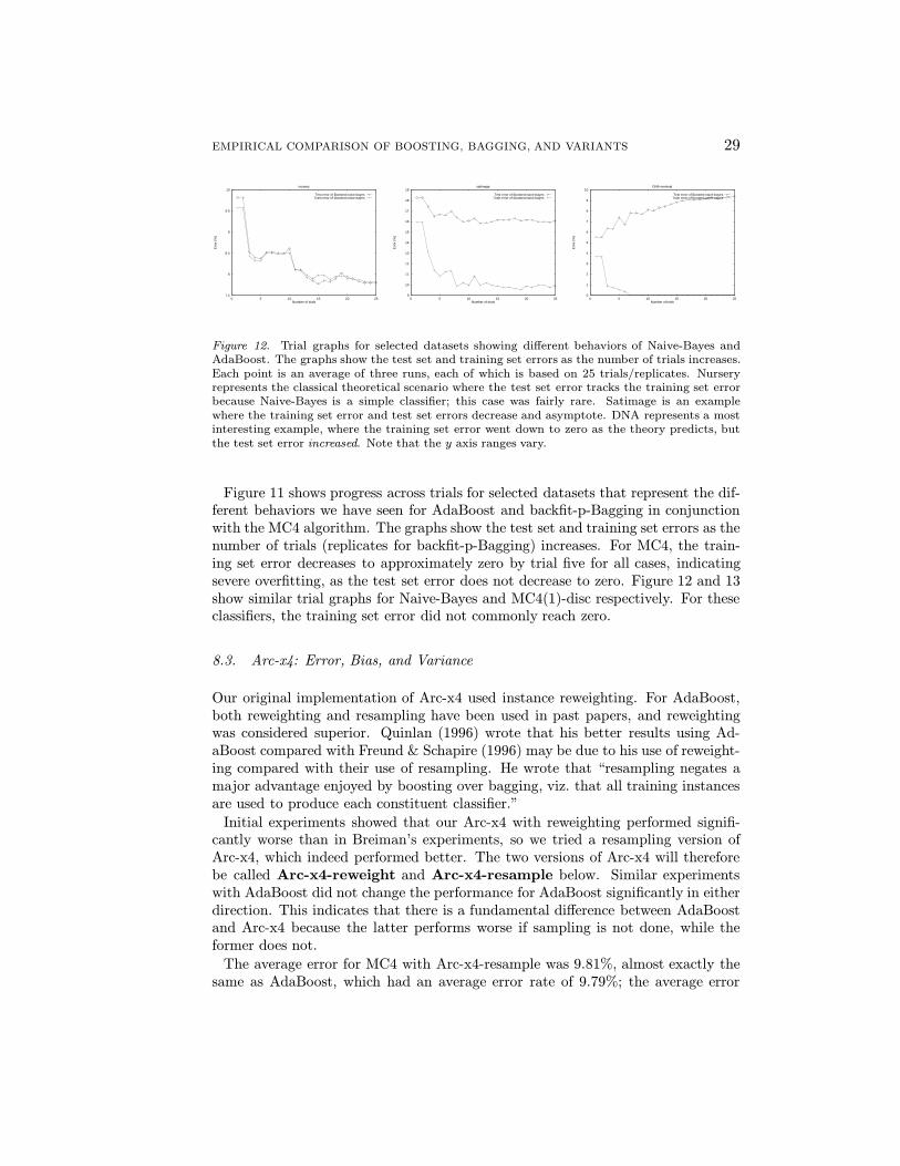
EMPIRICAL COMPARISON OF BOOSTING, BAGGING, AND VARIANTS 29
7.5
8
8.5
9
9.5
10
0 5 10 15 20 25
Err
or (
%)
Number of trials
nursery
Test error of Boosted naive-bayesTrain error of Boosted naive-bayes
9
10
11
12
13
14
15
16
17
18
19
0 5 10 15 20 25
Err
or (
%)
Number of trials
satimage
Test error of Boosted naive-bayesTrain error of Boosted naive-bayes
0
1
2
3
4
5
6
7
8
9
10
0 5 10 15 20 25
Err
or (
%)
Number of trials
DNA-nominal
Test error of Boosted naive-bayesTrain error of Boosted naive-bayes
Figure 12. Trial graphs for selected datasets showing different behaviors of Naive-Bayes andAdaBoost. The graphs show the test set and training set errors as the number of trials increases.Each point is an average of three runs, each of which is based on 25 trials/replicates. Nurseryrepresents the classical theoretical scenario where the test set error tracks the training set errorbecause Naive-Bayes is a simple classifier; this case was fairly rare. Satimage is an examplewhere the training set error and test set errors decrease and asymptote. DNA represents a mostinteresting example, where the training set error went down to zero as the theory predicts, butthe test set error increased. Note that the y axis ranges vary.
Figure 11 shows progress across trials for selected datasets that represent the dif-ferent behaviors we have seen for AdaBoost and backfit-p-Bagging in conjunctionwith the MC4 algorithm. The graphs show the test set and training set errors as thenumber of trials (replicates for backfit-p-Bagging) increases. For MC4, the train-ing set error decreases to approximately zero by trial five for all cases, indicatingsevere overfitting, as the test set error does not decrease to zero. Figure 12 and 13show similar trial graphs for Naive-Bayes and MC4(1)-disc respectively. For theseclassifiers, the training set error did not commonly reach zero.
8.3. Arc-x4: Error, Bias, and Variance
Our original implementation of Arc-x4 used instance reweighting. For AdaBoost,both reweighting and resampling have been used in past papers, and reweightingwas considered superior. Quinlan (1996) wrote that his better results using Ad-aBoost compared with Freund & Schapire (1996) may be due to his use of reweight-ing compared with their use of resampling. He wrote that “resampling negates amajor advantage enjoyed by boosting over bagging, viz. that all training instancesare used to produce each constituent classifier.”
Initial experiments showed that our Arc-x4 with reweighting performed signifi-cantly worse than in Breiman’s experiments, so we tried a resampling version ofArc-x4, which indeed performed better. The two versions of Arc-x4 will thereforebe called Arc-x4-reweight and Arc-x4-resample below. Similar experimentswith AdaBoost did not change the performance for AdaBoost significantly in eitherdirection. This indicates that there is a fundamental difference between AdaBoostand Arc-x4 because the latter performs worse if sampling is not done, while theformer does not.
The average error for MC4 with Arc-x4-resample was 9.81%, almost exactly thesame as AdaBoost, which had an average error rate of 9.79%; the average error
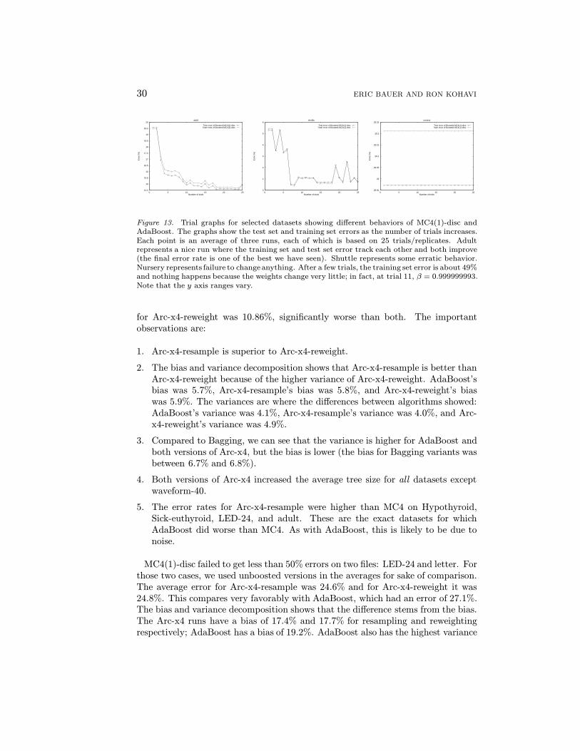
30 ERIC BAUER AND RON KOHAVI
14.5
15
15.5
16
16.5
17
17.5
18
18.5
19
19.5
20
0 5 10 15 20 25
Err
or (
%)
Number of trials
adult
Test error of Boosted MC4(1)-discTrain error of Boosted MC4(1)-disc
0
1
2
3
4
5
6
0 5 10 15 20 25
Err
or (
%)
Number of trials
shuttle
Test error of Boosted MC4(1)-discTrain error of Boosted MC4(1)-disc
28.95
29
29.05
29.1
29.15
29.2
29.25
0 5 10 15 20 25
Err
or (
%)
Number of trials
nursery
Test error of Boosted MC4(1)-discTrain error of Boosted MC4(1)-disc
Figure 13. Trial graphs for selected datasets showing different behaviors of MC4(1)-disc andAdaBoost. The graphs show the test set and training set errors as the number of trials increases.Each point is an average of three runs, each of which is based on 25 trials/replicates. Adultrepresents a nice run where the training set and test set error track each other and both improve(the final error rate is one of the best we have seen). Shuttle represents some erratic behavior.Nursery represents failure to change anything. After a few trials, the training set error is about 49%and nothing happens because the weights change very little; in fact, at trial 11, β = 0.999999993.Note that the y axis ranges vary.
for Arc-x4-reweight was 10.86%, significantly worse than both. The importantobservations are:
1. Arc-x4-resample is superior to Arc-x4-reweight.
2. The bias and variance decomposition shows that Arc-x4-resample is better thanArc-x4-reweight because of the higher variance of Arc-x4-reweight. AdaBoost’sbias was 5.7%, Arc-x4-resample’s bias was 5.8%, and Arc-x4-reweight’s biaswas 5.9%. The variances are where the differences between algorithms showed:AdaBoost’s variance was 4.1%, Arc-x4-resample’s variance was 4.0%, and Arc-x4-reweight’s variance was 4.9%.
3. Compared to Bagging, we can see that the variance is higher for AdaBoost andboth versions of Arc-x4, but the bias is lower (the bias for Bagging variants wasbetween 6.7% and 6.8%).
4. Both versions of Arc-x4 increased the average tree size for all datasets exceptwaveform-40.
5. The error rates for Arc-x4-resample were higher than MC4 on Hypothyroid,Sick-euthyroid, LED-24, and adult. These are the exact datasets for whichAdaBoost did worse than MC4. As with AdaBoost, this is likely to be due tonoise.
MC4(1)-disc failed to get less than 50% errors on two files: LED-24 and letter. Forthose two cases, we used unboosted versions in the averages for sake of comparison.The average error for Arc-x4-resample was 24.6% and for Arc-x4-reweight it was24.8%. This compares very favorably with AdaBoost, which had an error of 27.1%.The bias and variance decomposition shows that the difference stems from the bias.The Arc-x4 runs have a bias of 17.4% and 17.7% for resampling and reweightingrespectively; AdaBoost has a bias of 19.2%. AdaBoost also has the highest variance

EMPIRICAL COMPARISON OF BOOSTING, BAGGING, AND VARIANTS 31
(7.9%), while Arc-x4-resample has a variance of 7.2% and Arc-x4-reweight has avariance of 7.1%.
For Naive-Bayes, the average absolute error for Arc-x4-resample was 12.1% andthe average absolute error for Arc-x4-reweight was 12.3%; AdaBoost had an errorof 12.3% and Naive-Bayes had an error of 13.6%. As for MC4(1)-disc, the biasfor Arc-x4-resample is the lowest: 8.2%, followed with with Arc-x4-reweight andAdaBoost, which both have an error of 8.7%. For variance, Naive-Bayes itself isthe clear winner with 2.8%, followed by AdaBoost with 3.5%, then Arc-x4-reweightwith 3.6%, and Arc-x4-resample with 3.8%. As with MC4(1)-disc, Arc-x4-resampleslightly outperformed AdaBoost.
To summarize, Arc-x4-resample was superior to Arc-x4-reweight, and also out-performed AdaBoost for one level decision trees and Naive-Bayes. Both Arc-x4algorithms increased the variance for Naive-Bayes, but decreased the overall errordue to strong bias reductions.
8.4. Conclusions for Boosting
The AdaBoost and Arc-x4 algorithms have different behavior than Bagging, andthey also differ themselves. Here are the important observations:
1. On average, AdaBoost and Arc-x4-resample are better than Bagging for ourdatasets. This confirms previous comparisons (Breiman 1996a, Quinlan 1996).
2. AdaBoost and Arc-x4, however, are not uniformly better than Bagging. Therewere several cases where the performance of the boosting algorithms degradedcompared to the original (non-voted) algorithms. For MC4 and AdaBoost, these“failures” correlate well with the average decision-tree growth size relative tothe original trees. The Arc-x4 variants almost always increased the average treesize.
3. AdaBoost does not deal well with noise (this was also mentioned in Quinlan(1996)).
4. AdaBoost and Arc-x4 reduced both bias and variance for the decision treemethods. However, both algorithms increased the variance for Naive-Bayes(but still reduced the overall error).
5. For MC4(1)-disc, Breiman’s “ad hoc” algorithm works better than AdaBoost.
6. Arc-x4 and AdaBoost behave differently when sampling is applied. Arc-x4-resample outperformed Arc-x4-reweight, but for AdaBoost the result was thesame. The fact that Arc-x4 works as well as AdaBoost reinforces the hypothesisby Breiman (1996a) that the main benefit of AdaBoost can be attributed tothe adaptive reweighting.
7. The boosting theory guarantees that the training set error will go to zero. Thisscenario happens with MC4 but not with Naive-Bayes and MC4(1)-disc (seeFigure 12 and 13). In some cases we have observed errors very close to 0.5after several trials (e.g., the nursery dataset with MC4(1)-disc described above,
32 ERIC BAUER AND RON KOHAVI
DNA, and satimage). This is expected because boosting concentrates the weighton hard-to-classify instances, making the problem harder. In those cases therequirement that the error be bounded away from 0.5 is unsatisfied. In others,the improvement is so miniscule that many more boosting trials are apparentlyneeded (by orders of magnitude).
8. Unlike Bagging, where there was a significant difference between the combineddecision tree classifier making probabilistic or non-probabilistic predictions forcalculating the mean-squared error (MSE), AdaBoost was not significantlydifferent—less than 0.1%. AdaBoost is optimizing classification error and maybe too biased as a probability estimator.
With Bagging, we found that disabling pruning sometimes reduced the errors.With boosting it increased them. Using probabilistic estimates in the final com-bination was also slightly worse than using the classifications themselves. This isprobably due to the fact that all the reweighting that is done is based on classifi-cation errors. Finally, we did try to reweight instances based on the probabilisticpredictions of the classifiers as mentioned in Freund & Schapire (1995), but thatdid not work well either.
9. Future Work
Our study highlighted some problems in voting algorithms using error estima-tion, the bias and variance decomposition, average tree sizes, and graphs showingprogress over trials. While we made several new observations that clarify the be-havior of the algorithms, there are still some issues that require investigation infuture research.
1. The main problem with boosting seems to be robustness to noise. We attemptedto drop instances with very high weight but the experiments did not show this tobe a successful approach. Should smaller sample sizes be used to force theoriesto be simple if tree sizes grow as trials progress? Are there methods to makeboosting algorithms more robust when the dataset is noisy?
2. It is unclear how the tree size is affected in the different variants. AdaBoostseemed to have an interesting correlation between the change in average treesize and error reduction, but Arc-x4-resample did not have a similar correlation.Further research should try to explain the relations.
3. Boosting stops if one of the classifiers achieves zero training set error. Thatclassifier gets infinite voting power and is effectively the single classifier. Arethere better methods for handling this extreme situation?
4. In the case of the shuttle dataset, a single decision tree was built that wassignificantly better than the original MC4 tree. The decision tree had zero erroron the training set and thus became the only voter. Are there more situationswhen this is true, i.e., where one of the classifiers that was learned from a samplewith a skewed distribution performs well by itself on the unskewed test set?
EMPIRICAL COMPARISON OF BOOSTING, BAGGING, AND VARIANTS 33
5. Boosting and Bagging both create very complex classifiers, yet they do notseem to “overfit” the data. Domingos (1997) claims that the multiple treesdo not simply implement a Bayesian approach, but actually shift the learner’sbias (machine learning bias, not statistical bias) away from the commonly usedsimplicity bias. Can this bias be made more explicit?
6. We found that Bagging works well without pruning. Pruning in decision trees isa method for reducing the variance by introducing bias. Since Bagging reducesthe variance, disabling pruning indirectly reduces the bias. How does the errorrate change as pruning is increased? Specifically, are there cases where pruningshould still happen within Bagging?
7. Wolpert (1992) discusses stacking as a generic method for meta-learning. Bag-ging and Arc-x4 use uniform weighting, and AdaBoost uses a more complexweighting scheme. Is it possible that stacking another inducer might help? Weattempted to stack a Naive-Bayes on top of the base classifiers built by Ad-aBoost and Bagging without success. Can some better method to combineclassifiers be devised?
8. How can boosting be applied to other algorithms, such as k-nearest-neighbors?On the surface, the standard interpretation of counting a highly weighted in-stance more would not work, as increasing the weight of an instance helps toclassify its neighbors, not to classify itself.
9. Could probabilistic predictions made by the sub-classifiers be used? Quinlan(1996) used it as the voting strength, but this ignores the fact that the classifierswere built using skewed distributions.
10. Voting techniques usually result in incomprehensible classifiers that cannoteasily be shown to users. One solution proposed by Kohavi & Kunz (1997)attempts to build a structured model that has the same affect as Bagging.Ridgeway, Madigan & Richardson (1998) convert a boosted Naive-Bayes toa regular Naive-Bayes, which then allows for visualizations (Becker, Kohavi &Sommerfield 1997). Are there ways to make boosting comprehensible for generalmodels? Craven & Shavlik (1993) built a single decision tree that attempts tomake the same classifications as a neural network. Quinlan (1994) notes thatthere are parallel problems that require testing all attributes. A single tree forsuch problems must be large.
11. In parallel environments, Bagging has a strong advantage because the sub-classifiers can be built in parallel. Boosting methods, on the other hand, requirethe estimated training set error on trial T to generate the distribution for trialT + 1. This makes coarse-grain parallelization very hard. Can some efficientparallel implementations be devised?
34 ERIC BAUER AND RON KOHAVI
10. Conclusions
We provided a brief review of two families of voting algorithms: perturb and com-bine (e.g., Bagging), and boosting (e.g., AdaBoost, Arc-x4). Our contributionsinclude:
1. A large-scale comparison of Bagging, Bagging variants, AdaBoost, and Arc-x4on two families of induction algorithms: decision trees and Naive-Bayes. Manyprevious papers have concentrated on a few datasets where the performanceof Bagging and AdaBoost was stellar. We believe that this paper gives a morerealistic view of the performance improvement one can expect. Specifically, withthe best algorithm, AdaBoost, the average relative error reduction was 27% forMC4, 31% for MC4(1)-disc, and 24% for Naive-Bayes. The boosting algorithmswere generally better than Bagging, but not uniformly better. Furthermore, insome datasets (e.g., adult) none of the voting algorithms helped, even thoughwe knew from the learning curve graphs that the Bayes optimal error was lower.
2. A decomposition of the error rates into bias and variance for real datasets. Pre-vious work that provided this decomposition did so only for artificial datasets.We believe that our decomposition on real-world problems is more informa-tive and leads to a better understanding of the tradeoffs involved in real-worldscenarios. Bagging’s error reduction in conjunction with MC4 is mostly due tovariance reduction because MC4 is unstable and has high variance. For MC4(1)and MC4(1)-disc, Bagging reduced the bias more significantly than the variance.Bagging had little effect on Naive-Bayes. The boosting methods reduced boththe bias and the variance.
3. An evaluation of several variants of voting algorithms, including no-pruning,probabilistic variants, and backfitting. These were shown to outperform theoriginal Bagging algorithm.
4. A mean-squared error evaluation showed that voting techniques are extremelysuccessful at reducing the loss under this metric. We believe that voting tech-niques should perform significantly better when loss matrices are used, whichis fairly common in real-world applications.
5. A discussion of numerical instabilities, which require careful thought in imple-mentation of boosting algorithms.
6. A positive correlation between the increase in the average tree size in AdaBoosttrials and its success in reducing the error.
7. An observation that Arc-x4 does not work as well with reweighting methods;rather, unlike AdaBoost, the sampling step is crucial.
The error rates we achieved with Bagging and the boosting algorithms were some-times surprisingly good. Looking at the learning curves, the voting algorithms builtclassifiers from small samples that outperformed what looked like the asymptoticerror for the original algorithms. For example, Waveform seemed to have stabilizedaround an error of 20% when the training set size was 3,000-4,500 instances, yet
EMPIRICAL COMPARISON OF BOOSTING, BAGGING, AND VARIANTS 35
AdaBoost had a 17.7% error rate with training set sizes of 1,000 instances. For theLetter domain, the lowest error on the learning curve was about 12% for 18,000instances, yet AdaBoost had an error rate of 8.1% with a training set size of 5,000.
For learning tasks where comprehensibility is not crucial, voting methods areextremely useful, and we expect to see them used significantly more than they aretoday.
Acknowledgments
Eric Bauer interned at Silicon Graphics when this work was done. The researchwas conducted using MLC++, which is available freely for research purposes. Wethank Carla Brodley, Cliff Brunk, Tom Dietterich, Eric Eros, Clay Kunz, FosterProvost, and Ross Quinlan, for their helpful comments on a draft of this paper.We also thank Yoav Freund and Rob Schapire for clarifying some issues with theAdaBoost algorithm. Special thanks to those at Silicon Graphics who let us usesome powerful servers for this work, including Uday Hegde and Steve Whitney fromthe Scalable Networked Servers division, Lori Gilbertson from the Cray Researchsubsidiary, and Eugene Yu from Manufacturing. We estimate that about 4,000CPU hours (MIPS 195Mhz R10K) were used in this study. Such a study couldnot easily be done without those 32, 64, and 128 CPU Origin 2000s with dozens ofgigabytes of RAM. We will always remember CPU #55 on flurry.
Notes
1. The original boosting algorithm weights instances so that the total weight of the sample is one.Due to numerical instabilities, we assign an initial weight of one to each instance and normalizeto the number of instances as described in Section 8.1. There is no algorithmic difference here.
References
Ali, K. M. (1996), Learning Probabilistic Relational Concept Descriptions, PhD thesis, Universityof California, Irvine. http://www.ics.uci.edu/˜ali.
Becker, B., Kohavi, R. & Sommerfield, D. (1997), Visualizing the simple bayesian classifier, in‘KDD Workshop on Issues in the Integration of Data Mining and Data Visualization’.
Bernardo, J. M. & Smith, A. F. (1993), Bayesian Theory, John Wiley & Sons.Breiman, L. (1994), Heuristics of instability in model selection, Technical Report Statistics De-
partment, University of California at Berkeley.Breiman, L. (1996a), Arcing classifiers, Technical report, Statistics Department, University of
California, Berkeley.http://www.stat.Berkeley.EDU/users/breiman/.
Breiman, L. (1996b), ‘Bagging predictors’, Machine Learning 24, 123–140.Breiman, L. (1997), Arcing the edge, Technical Report Technical Report 486, Statistics Depart-
ment, University of California, Berkeley.http://www.stat.Berkeley.EDU/users/breiman/.
Buntine, W. (1992a), ‘Learning classification trees’, Statistics and Computing 2(2), 63–73.Buntine, W. (1992b), A Theory of Learning Classification Rules, PhD thesis, University of Tech-
nology, Sydney, School of Computing Science.C. Blake, E. K. & Merz, C. (1998), ‘UCI repository of machine learning databases’.
http://www.ics.uci.edu/∼mlearn/MLRepository.html.

36 ERIC BAUER AND RON KOHAVI
Cestnik, B. (1990), Estimating probabilities: A crucial task in machine learning, in L. C. Aiello,ed., ‘Proceedings of the ninth European Conference on Artificial Intelligence’, pp. 147–149.
Chan, P., Stolfo, S. & Wolpert, D. (1996), Integrating multiple learned models for improving andscaling machine learning algorithms. AAAI Workshop.
Craven, M. W. & Shavlik, J. W. (1993), Learning symbolic rules using artificial neural networks,in ‘Proceedings of the Tenth International Conference on Machine Learning’, Morgan Kauf-mann, pp. 73–80.
Dietterich, T. G. (1998), ‘Approximate statistical tests for comparing supervised classificationlearning algorithms’, Neural Computation 10(7).
Dietterich, T. G. & Bakiri, G. (1991), Error-correcting output codes: A general method forimproving multiclass inductive learning programs, in ‘Proceedings of the Ninth NationalConference on Artificial Intelligence (AAAI-91)’, pp. 572–577.
Domingos, P. (1997), Why does bagging work? a Bayesian account and its implications, inD. Heckerman, H. Mannila, D. Pregibon & R. Uthurusamy, eds, ‘Proceedings of the thirdinternational conference on Knowledge Discovery and Data Mining’, AAAI Press, pp. 155–158.
Domingos, P. & Pazzani, M. (1997), ‘Beyond independence: Conditions for the optimality of thesimple Bayesian classifier’, Machine Learning 29(2/3), 103–130.
Drucker, H. & Cortes, C. (1996), Boosting decision trees, in ‘Advances in Neural Informationprocessing Systems 8’, pp. 479–485.
Duda, R. & Hart, P. (1973), Pattern Classification and Scene Analysis, Wiley.Efron, B. & Tibshirani, R. (1993), An Introduction to the Bootstrap, Chapman & Hall.Elkan, C. (1997), Boosting and Naive Bayesian learning, Technical report, Department of Com-
puter Science and Engineering, University of California, San Diego.Fayyad, U. M. & Irani, K. B. (1993), Multi-interval discretization of continuous-valued attributes
for classification learning, in ‘Proceedings of the 13th International Joint Conference onArtificial Intelligence’, Morgan Kaufmann Publishers, Inc., pp. 1022–1027.
Freund, Y. (1990), Boosting a weak learning algorithm by majority, in ‘Proceedings of the ThirdAnnual Workshop on Computational Learning Theory’, pp. 202–216.
Freund, Y. (1996), ‘Boosting a weak learning algorithm by majority’, Information and Computa-tion 121(2), 256–285.
Freund, Y. & Schapire, R. E. (1995), A decision-theoretic generalization of on-line learning andan application to boosting, in ‘Proceedings of the Second European Conference on Compu-tational Learning Theory’, Springer-Verlag, pp. 23–37. To appear in Journal of Computerand System Sciences.
Freund, Y. & Schapire, R. E. (1996), Experiments with a new boosting algorithm, in L. Saitta, ed.,‘Machine Learning: Proceedings of the Thirteenth National Conference’, Morgan Kaufmann,pp. 148–156.
Friedman, J. H. (1997), ‘On bias, variance, 0/1-loss, and the curse of dimensionality’, Data Miningand Knowledge Discovery 1(1), 55–77.ftp://playfair.stanford.edu/pub/friedman/curse.ps.Z.
Geman, S., Bienenstock, E. & Doursat, R. (1992), ‘Neural networks and the bias/variancedilemma’, Neural Computation 4, 1–48.
Good, I. J. (1965), The Estimation of Probabilities: An Essay on Modern Bayesian Methods,M.I.T. Press.
Holte, R. C. (1993), ‘Very simple classification rules perform well on most commonly useddatasets’, Machine Learning 11, 63–90.
Iba, W. & Langley, P. (1992), Induction of one-level decision trees, in ‘Proceedings of the NinthInternational Conference on Machine Learning’, Morgan Kaufmann Publishers, Inc., pp. 233–240.
Kohavi, R. (1995a), A study of cross-validation and bootstrap for accuracy estimation and modelselection, in C. S. Mellish, ed., ‘Proceedings of the 14th International Joint Conference onArtificial Intelligence’, Morgan Kaufmann, pp. 1137–1143.http://robotics.stanford.edu/~ronnyk.
Kohavi, R. (1995b), Wrappers for Performance Enhancement and Oblivious Decision Graphs, PhDthesis, Stanford University, Computer Science department. STAN-CS-TR-95-1560,http://robotics.Stanford.EDU/˜ronnyk/teza.ps.Z.
EMPIRICAL COMPARISON OF BOOSTING, BAGGING, AND VARIANTS 37
Kohavi, R., Becker, B. & Sommerfield, D. (1997), Improving Simple Bayes, in ‘The 9th EuropeanConference on Machine Learning, Poster Papers’, pp. 78–87. Available athttp://robotics.stanford.edu/users/ronnyk.
Kohavi, R. & Kunz, C. (1997), Option decision trees with majority votes, in D. Fisher, ed., ‘Ma-chine Learning: Proceedings of the Fourteenth International Conference’, Morgan KaufmannPublishers, Inc., pp. 161–169. Available athttp://robotics.stanford.edu/users/ronnyk.
Kohavi, R. & Sahami, M. (1996), Error-based and entropy-based discretization of continuousfeatures, in ‘Proceedings of the Second International Conference on Knowledge Discoveryand Data Mining’, pp. 114–119.
Kohavi, R. & Sommerfield, D. (1995), Feature subset selection using the wrapper model: Overfit-ting and dynamic search space topology, in ‘The First International Conference on KnowledgeDiscovery and Data Mining’, pp. 192–197.
Kohavi, R., Sommerfield, D. & Dougherty, J. (1997), ‘Data mining using MLC++: A machinelearning library in C++’, International Journal on Artificial Intelligence Tools 6(4), 537–566.http://www.sgi.com/Technology/mlc.
Kohavi, R. & Wolpert, D. H. (1996), Bias plus variance decomposition for zero-oneloss functions, in L. Saitta, ed., ‘Machine Learning: Proceedings of the Thir-teenth International Conference’, Morgan Kaufmann, pp. 275–283. Available athttp://robotics.stanford.edu/users/ronnyk.
Kong, E. B. & Dietterich, T. G. (1995), Error-correcting output coding corrects bias and variance,in A. Prieditis & S. Russell, eds, ‘Machine Learning: Proceedings of the Twelfth InternationalConference’, Morgan Kaufmann, pp. 313–321.
Kwok, S. W. & Carter, C. (1990), Multiple decision trees, in R. D. Schachter, T. S. Levitt,L. N. Kanal & J. F. Lemmer, eds, ‘Uncertainty in Artificial Intelligence’, Elsevier SciencePublishers, pp. 327–335.
Langley, P., Iba, W. & Thompson, K. (1992), An analysis of Bayesian classifiers, in ‘Proceedings ofthe tenth national conference on artificial intelligence’, AAAI Press and MIT Press, pp. 223–228.
Langley, P. & Sage, S. (1997), Scaling to domains with many irrelevant features, in R. Greiner,ed., ‘Computational Learning Theory and Natural Learning Systems’, Vol. 4, MIT Press.
Oates, T. & Jensen, D. (1997), The effects of training set size on decision tree complexity, inD. Fisher, ed., ‘Machine Learning: Proceedings of the Fourteenth International Conference’,Morgan Kaufmann, pp. 254–262.
Oliver, J. & Hand, D. (1995), On pruning and averaging decision trees, in A. Prieditis & S. Rus-sell, eds, ‘Machine Learning: Proceedings of the Twelfth International Conference’, MorganKaufmann, pp. 430–437.
Pazzani, M., Merz, C., Murphy, P., Ali, K., Hume, T. & Brunk, C. (1994), Reducing misclassifi-cation costs, in ‘Machine Learning: Proceedings of the Eleventh International Conference’,Morgan Kaufmann.
Quinlan, J. R. (1993), C4.5: Programs for Machine Learning, Morgan Kaufmann, San Mateo,California.
Quinlan, J. R. (1994), Comparing connectionist and symbolic learning methods, in S. J. Hanson,G. A. Drastal & R. L. Rivest, eds, ‘Computational Learning Theory and Natural LearningSystems’, Vol. I: Constraints and Prospects, MIT Press, chapter 15, pp. 445—456.
Quinlan, J. R. (1996), Bagging, boosting, and c4.5, in ‘Proceedings of the Thirteenth NationalConference on Artificial Intelligence’, AAAI Press and the MIT Press, pp. 725–730.
Ridgeway, G., Madigan, D. & Richardson, T. (1998), Interpretable boosted naive bayes classifi-cation, in ‘Proceedings of the Fourth International Conference on Knowledge Discovery andData Mining’.
Schaffer, C. (1994), A conservation law for generalization performance, in ‘Machine Learning:Proceedings of the Eleventh International Conference’, Morgan Kaufmann, pp. 259–265.
Schapire, R. E. (1990), ‘The strength of weak learnability’, Machine Learning 5(2), 197–227.Schapire, R. E., Freund, Y., Bartlett, P. & Lee, W. S. (1997), Boosting the margin: A new
explanation for the effectiveness of voting methods, in D. Fisher, ed., ‘Machine Learning:Proceedings of the Fourteenth International Conference’, Morgan Kaufmann, pp. 322–330.
38 ERIC BAUER AND RON KOHAVI
Wolpert, D. H. (1992), ‘Stacked generalization’, Neural Networks 5, 241–259.Wolpert, D. H. (1994), The relationship between PAC, the statistical physics framework, the
Bayesian framework, and the VC framework, in D. H. Wolpert, ed., ‘The Mathematics ofGeneralization’, Addison Wesley.