An empirical comparison of the runtime of five sorting ...uploads.julianapena.com/ib-ee.pdf · An...

INTERNATIONAL BACCALAUREATE EXTENDED ESSAY

An empirical comparison of the runtime of five sorting algorithms

Topic: Algorithms

Subject: Computer Science

Juliana Peña Ocampo

Candidate Number: D 000033-049

Number Of Words: 3028

COLEGIO COLOMBO BRITÁNICO

Santiago De Cali

Colombia

2008

Juliana Peña Ocampo – 000033-049

2/26

Abstract

Sorting algorithms are of extreme importance in the field of Computer Science because of the amount of time computers spend on the process of sorting. Sorting is used by almost every application as an intermediate step to other processes, such as searching. By optimizing sorting, computing as a whole will be faster.

The basic process of sorting is the same: taking a list of items, and producing a permutation of the same list in arranged in a prescribed non-decreasing order. There are, however, varying methods or algorithms which can be used to achieve this. Amongst them are bubble sort, selection sort, insertion sort, Shell sort, and Quicksort.

The purpose of this investigation is to determine which of these algorithms is the fastest to sort lists of different lengths, and to therefore determine which algorithm should be used depending on the list length. Although asymptotic analysis of the algorithms is touched upon, the main type of comparison discussed is an empirical assessment based on running each algorithm against random lists of different sizes.

Through this study, a conclusion can be brought on what algorithm to use in each particular occasion. Shell sort should be used for all sorting of small (less than 1000 items) arrays. It has the advantage of being an in-place and non-recursive algorithm, and is faster than Quicksort up to a certain point. For larger arrays, the best choice is Quicksort, which uses recursion to sort lists, leading to higher system usage but significantly faster results.

However, an algorithmic study based on time of execution of sorting random lists alone is not complete. Other factors must be taken into account in order to guarantee a high-quality product. These include, but are not limited to, list type, memory footprint, CPU usage, and algorithm correctness.


3/26

Table of Contents

Abstract ........................................................................................................................................... 2

1. Introduction ............................................................................................................................. 4

2. Objective .................................................................................................................................. 4

3. The importance of sorting ....................................................................................................... 5

4. Classification of sorting algorithms ......................................................................................... 6

5. A brief explanation of each algorithm ..................................................................................... 7

5.1. The bubble sort algorithm ................................................................................................ 7

5.2. The selection sort algorithm ............................................................................................. 8

5.3. The insertion sort algorithm ............................................................................................. 9

5.4. The Shell sort algorithm .................................................................................................. 10

5.5. The Quicksort algorithm ................................................................................................. 12

6. Analytical Comparison ........................................................................................................... 13

7. Empirical comparison ............................................................................................................ 14

7.1. Tests made ...................................................................................................................... 14

7.2. Results ............................................................................................................................. 15

7.2.1. Total Results ............................................................................................................ 15

7.2.2. Average Results ....................................................................................................... 17

8. Conclusions and Evaluation ................................................................................................... 19

8.1. Conclusions ..................................................................................................................... 19

8.2. Evaluation ....................................................................................................................... 20

8.2.1. Limitations of an empirical comparison ...................................................................... 20

8.2.2. Limitation of a runtime-based comparison ................................................................ 20

8.2.3. Limitations of a comparison based on random arrays ............................................... 20

8.2.4. Exploration of other types of algorithms .................................................................... 21

Bibliography ................................................................................................................................... 22

Appendix A: Python Source Code for the Algorithms, Shuffler and Timer ................................... 23

Appendix B: Contents of the output file, out.txt ........................................................................... 26


4/26

1. Introduction

Sorting is one of the most important operations computers perform on data. Together with another equally important operation, searching, it is probably the most used algorithm in computing, and one in which, statistically, computers spend around half of the time performing1. For this reason, the development of fast, efficient and inexpensive algorithms for sorting and ordering lists and arrays is a fundamental field of computing. The study of the different types of sorting algorithms depending on list lengths will lead to faster and more efficient software when conclusions are drawn on what algorithm to use on which context. What is the best algorithm to use on short lists? Is that algorithm as efficient with short lists as it is with long lists? If not, which algorithm could then be used for longer lists? These are some of the questions that will be explored in this investigation.

2. Objective

The purpose of this investigation is to determine which algorithm requires the least amount of time to sort lists of different lengths, and to therefore determine which algorithm should be used depending on the list length.

Five different sorting algorithms will be studied and compared:

Bubble sort

Straight selection sort (called simply ´selection sort´ for the remainder of this investigation)

Linear insertion sort (called simply ´insertion sort´ for the remainder of this investigation)

Shell sort

Quicksort

All of these algorithms are comparison algorithms with a worst case runtime of 𝑂(𝑛2). All are in-place algorithms except for Quicksort which uses recursion. This experiment will seek to find which of these algorithms is fastest to sort random one-dimensional lists of sequential integers of varying size.

1 (Joyannes Aguilar, 2003, p. 360)


5/26

3. The importance of sorting

Sorting is one of the fundamental problems studied in computer science. Sorting is used on a daily basis in almost all operations regarding the process of information, from writing a phone number in an address book to compiling a list of guests to a party to organizing a music collection. Not only does sorting make information more human-readable, but it also makes searching and other processes much more efficient: it is much easier to search for words in the dictionary when they are in a pre-described alphabetical order, for example. As a more concrete example of how sorting aids searching, linear search can find items in an unsorted list of size 𝑛 in a maximum 𝑛 comparisons, while binary search, which only searches sorted lists, can find an item in at most 𝑙𝑜𝑔2𝑛 comparisons.

The basic objective of sorting is always the same: taking a list of unorganized items, and arranging them to a certain order. This order can vary, however: if the items in the list are contacts in an address book, for example, they can be organized alphabetically by last name, numerically by phone number, or chronologically by birthday, for instance. Still, the basic process is the same: taking the items and permuting them in a ‘non-decreasing order … according to a desired total order’2.

2 (Wikipedia contributors, 2007)


6/26

4. Classification of sorting algorithms

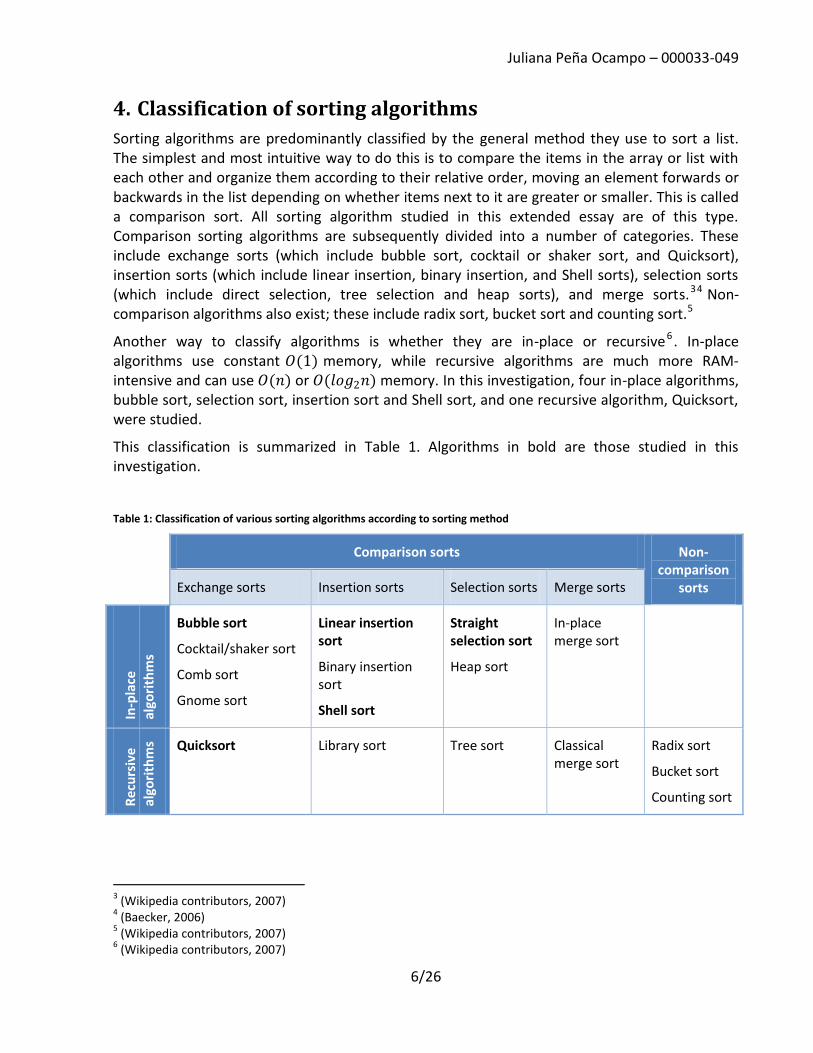
Sorting algorithms are predominantly classified by the general method they use to sort a list. The simplest and most intuitive way to do this is to compare the items in the array or list with each other and organize them according to their relative order, moving an element forwards or backwards in the list depending on whether items next to it are greater or smaller. This is called a comparison sort. All sorting algorithm studied in this extended essay are of this type. Comparison sorting algorithms are subsequently divided into a number of categories. These include exchange sorts (which include bubble sort, cocktail or shaker sort, and Quicksort), insertion sorts (which include linear insertion, binary insertion, and Shell sorts), selection sorts (which include direct selection, tree selection and heap sorts), and merge sorts.34 Non-comparison algorithms also exist; these include radix sort, bucket sort and counting sort.5

Another way to classify algorithms is whether they are in-place or recursive6 . In-place algorithms use constant 𝑂(1) memory, while recursive algorithms are much more RAM-intensive and can use 𝑂(𝑛) or 𝑂(𝑙𝑜𝑔2𝑛) memory. In this investigation, four in-place algorithms, bubble sort, selection sort, insertion sort and Shell sort, and one recursive algorithm, Quicksort, were studied.

This classification is summarized in Table 1. Algorithms in bold are those studied in this investigation.

Table 1: Classification of various sorting algorithms according to sorting method

Comparison sorts Non-comparison

sorts Exchange sorts Insertion sorts Selection sorts Merge sorts

In-p

lace

al

gori

thm

s

Bubble sort

Cocktail/shaker sort

Comb sort

Gnome sort

Linear insertion sort

Binary insertion sort

Shell sort

Straight selection sort

Heap sort

In-place merge sort

Re

curs

ive

algo

rith

ms Quicksort Library sort Tree sort Classical

merge sort Radix sort

Bucket sort

Counting sort


4 (Baecker, 2006)




7/26

5. A brief explanation of each algorithm

5.1. The bubble sort algorithm

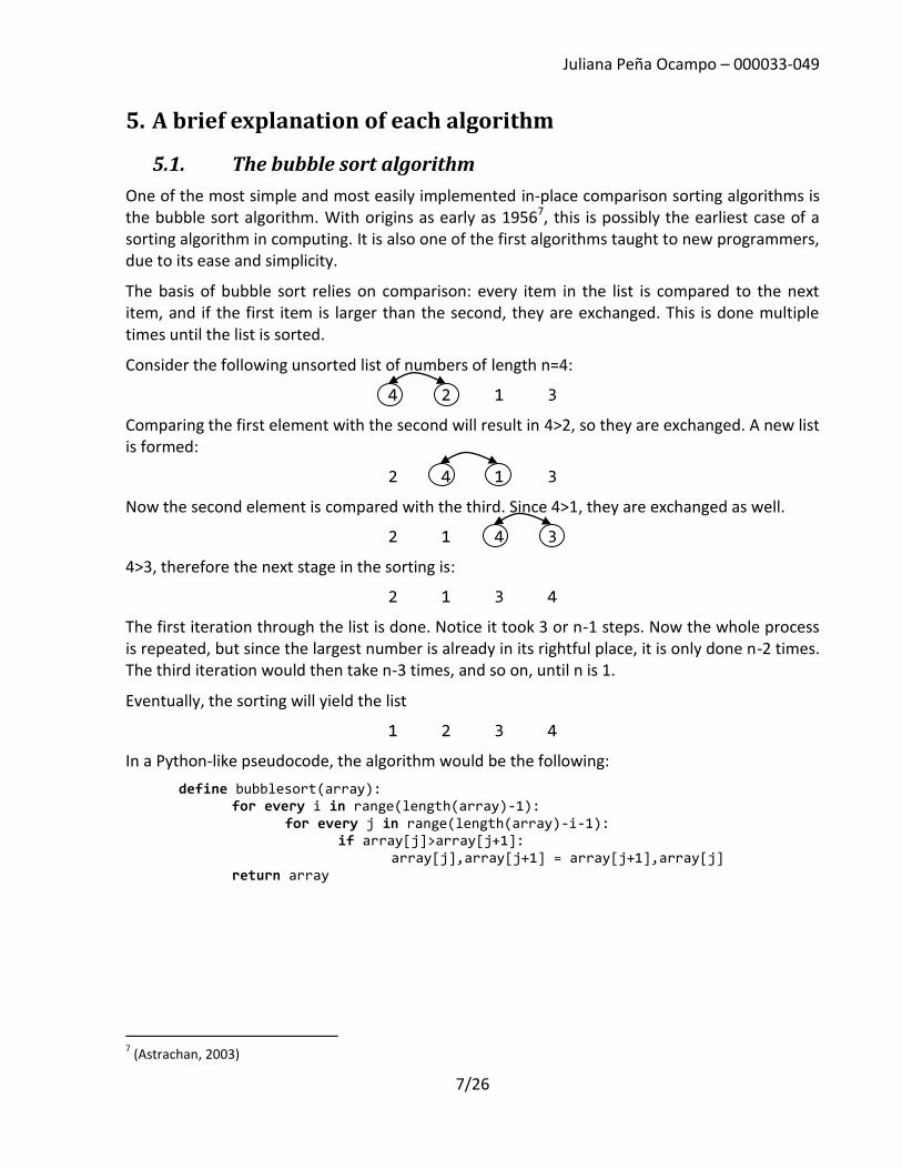
One of the most simple and most easily implemented in-place comparison sorting algorithms is the bubble sort algorithm. With origins as early as 19567, this is possibly the earliest case of a sorting algorithm in computing. It is also one of the first algorithms taught to new programmers, due to its ease and simplicity.

The basis of bubble sort relies on comparison: every item in the list is compared to the next item, and if the first item is larger than the second, they are exchanged. This is done multiple times until the list is sorted.

Consider the following unsorted list of numbers of length n=4:

4 2 1 3

Comparing the first element with the second will result in 4>2, so they are exchanged. A new list is formed:

2 4 1 3

Now the second element is compared with the third. Since 4>1, they are exchanged as well.

2 1 4 3

4>3, therefore the next stage in the sorting is:

2 1 3 4

The first iteration through the list is done. Notice it took 3 or n-1 steps. Now the whole process is repeated, but since the largest number is already in its rightful place, it is only done n-2 times. The third iteration would then take n-3 times, and so on, until n is 1.

Eventually, the sorting will yield the list

1 2 3 4

In a Python-like pseudocode, the algorithm would be the following:

define bubblesort(array): for every i in range(length(array)-1): for every j in range(length(array)-i-1): if array[j]>array[j+1]: array[j],array[j+1] = array[j+1],array[j] return array

7 (Astrachan, 2003)


8/26

5.2. The selection sort algorithm

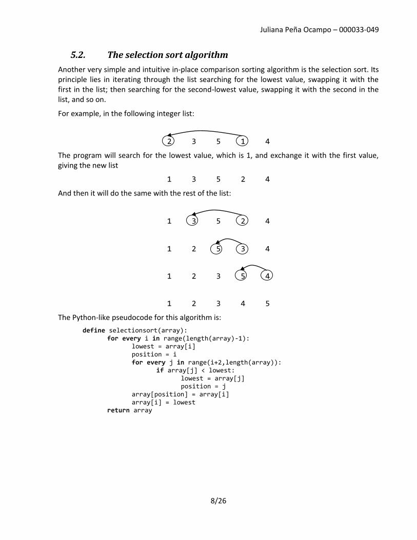
Another very simple and intuitive in-place comparison sorting algorithm is the selection sort. Its principle lies in iterating through the list searching for the lowest value, swapping it with the first in the list; then searching for the second-lowest value, swapping it with the second in the list, and so on.

For example, in the following integer list:

2 3 5 1 4

The program will search for the lowest value, which is 1, and exchange it with the first value, giving the new list

1 3 5 2 4

And then it will do the same with the rest of the list:

1 3 5 2 4

1 2 5 3 4

1 2 3 5 4

1 2 3 4 5

The Python-like pseudocode for this algorithm is:

define selectionsort(array): for every i in range(length(array)-1): lowest = array[i] position = i for every j in range(i+2,length(array)): if array[j] < lowest: lowest = array[j] position = j array[position] = array[i] array[i] = lowest return array


9/26

5.3. The insertion sort algorithm

Insertion sort is an in-place comparison sorting algorithm which works by selecting an item in

the list and inserting it in its correct position relative to the items sorted so far.

For example, in the following list:

3 5 2 1 4

The algorithm always starts with the second item (5 in this case) and classifies it according to

the items on the left shown in blue (only 3 in this case). Since it is already in its correct position

(3<5), it is not moved.

3 5 2 1 4

Now the same thing is done with 2. It is compared to the items to its left, 3 and 5. Since 2 < 3, it

is put to the left of 3:

2 3 5 1 4

The algorithm is repeated until all the items are in order:

2 3 5 1 4

1 < 2:

1 2 3 5 4

3 < 4 < 5:

1 2 3 4 5

The Python-like pseudocode for this algorithm is as follows:

define insertionsort(array): for every i in range(1,length(array)): value = array[i] j = i-1 while j>=0 and array[j]>value: array[j+1] = array[j] j-=1 array[j+1] = value return array


10/26

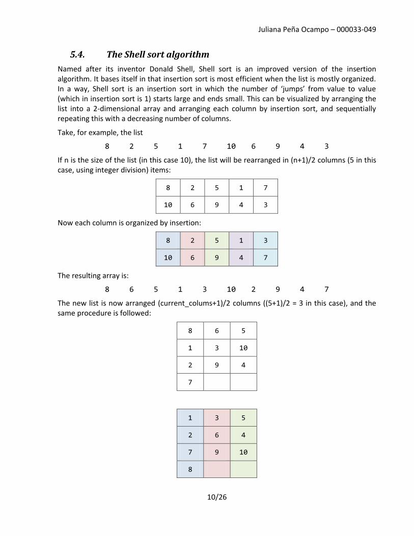
5.4. The Shell sort algorithm

Named after its inventor Donald Shell, Shell sort is an improved version of the insertion algorithm. It bases itself in that insertion sort is most efficient when the list is mostly organized. In a way, Shell sort is an insertion sort in which the number of ‘jumps’ from value to value (which in insertion sort is 1) starts large and ends small. This can be visualized by arranging the list into a 2-dimensional array and arranging each column by insertion sort, and sequentially repeating this with a decreasing number of columns.

Take, for example, the list

8 2 5 1 7 10 6 9 4 3

If n is the size of the list (in this case 10), the list will be rearranged in (n+1)/2 columns (5 in this case, using integer division) items:

8 2 5 1 7

10 6 9 4 3

Now each column is organized by insertion:

8 2 5 1 3

10 6 9 4 7

The resulting array is:

8 6 5 1 3 10 2 9 4 7

The new list is now arranged (current_colums+1)/2 columns ((5+1)/2 = 3 in this case), and the same procedure is followed:

8 6 5

1 3 10

2 9 4

7

1 3 5

2 6 4

7 9 10

8


11/26

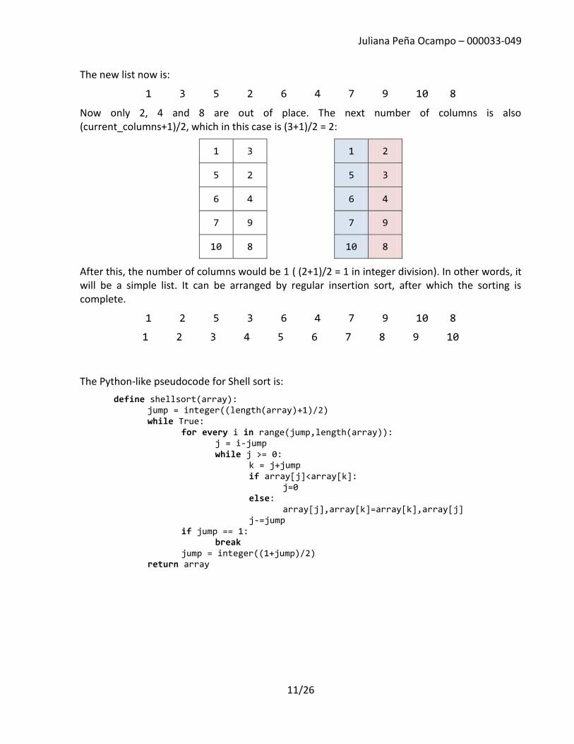
The new list now is:

1 3 5 2 6 4 7 9 10 8

Now only 2, 4 and 8 are out of place. The next number of columns is also (current_columns+1)/2, which in this case is (3+1)/2 = 2:

1 3 1 2

5 2 5 3

6 4 6 4

7 9 7 9

10 8 10 8

After this, the number of columns would be 1 ( (2+1)/2 = 1 in integer division). In other words, it will be a simple list. It can be arranged by regular insertion sort, after which the sorting is complete.

1 2 5 3 6 4 7 9 10 8

1 2 3 4 5 6 7 8 9 10

The Python-like pseudocode for Shell sort is:

define shellsort(array): jump = integer((length(array)+1)/2) while True: for every i in range(jump,length(array)): j = i-jump while j >= 0: k = j+jump if array[j]<array[k]: j=0 else: array[j],array[k]=array[k],array[j] j-=jump if jump == 1: break jump = integer((1+jump)/2) return array


12/26

5.5. The Quicksort algorithm

Quicksort is a recursive divide-and-conquer comparison sorting algorithm. It takes into account that small lists are easier to sort than long ones. Quicksort it known to be one of the fastest sorting algorithms; however, due to its recursive nature, it is much more hardware-intensive than in-place algorithms like Shell sort or selection sort.

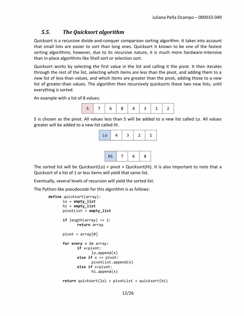
Quicksort works by selecting the first value in the list and calling it the pivot. It then iterates through the rest of the list, selecting which items are less than the pivot, and adding them to a new list of less-than values, and which items are greater than the pivot, adding those to a new list of greater-than values. The algorithm then recursively quicksorts these two new lists, until everything is sorted.

An example with a list of 8 values:

5 7 6 8 4 3 1 2

5 is chosen as the pivot. All values less than 5 will be added to a new list called Lo. All values greater will be added to a new list called Hi.

Lo 4 3 2 1

Hi 7 6 8

The sorted list will be Quicksort(Lo) + pivot + Quicksort(Hi). It is also important to note that a Quicksort of a list of 1 or less items will yield that same list.

Eventually, several levels of recursion will yield the sorted list.

The Python-like pseudocode for this algorithm is as follows:

define quicksort(array): lo = empty_list hi = empty_list pivotList = empty_list if length(array) <= 1: return array pivot = array[0] for every x in array: if x<pivot: lo.append(x) else if x == pivot: pivotList.append(x) else if x>pivot: hi.append(x) return quicksort(lo) + pivotList + quicksort(hi)


13/26

6. Analytical Comparison

A limitation of the empirical comparison is that it is system-dependent. A more effective way of comparing algorithms is through their time complexity upper bound to guarantee that an algorithm will run at most a certain time with order of magnitude 𝑂(𝑓(𝑛)), where 𝑛 is the number of items in the list to be sorted. This type of comparison is called asymptotic analysis.

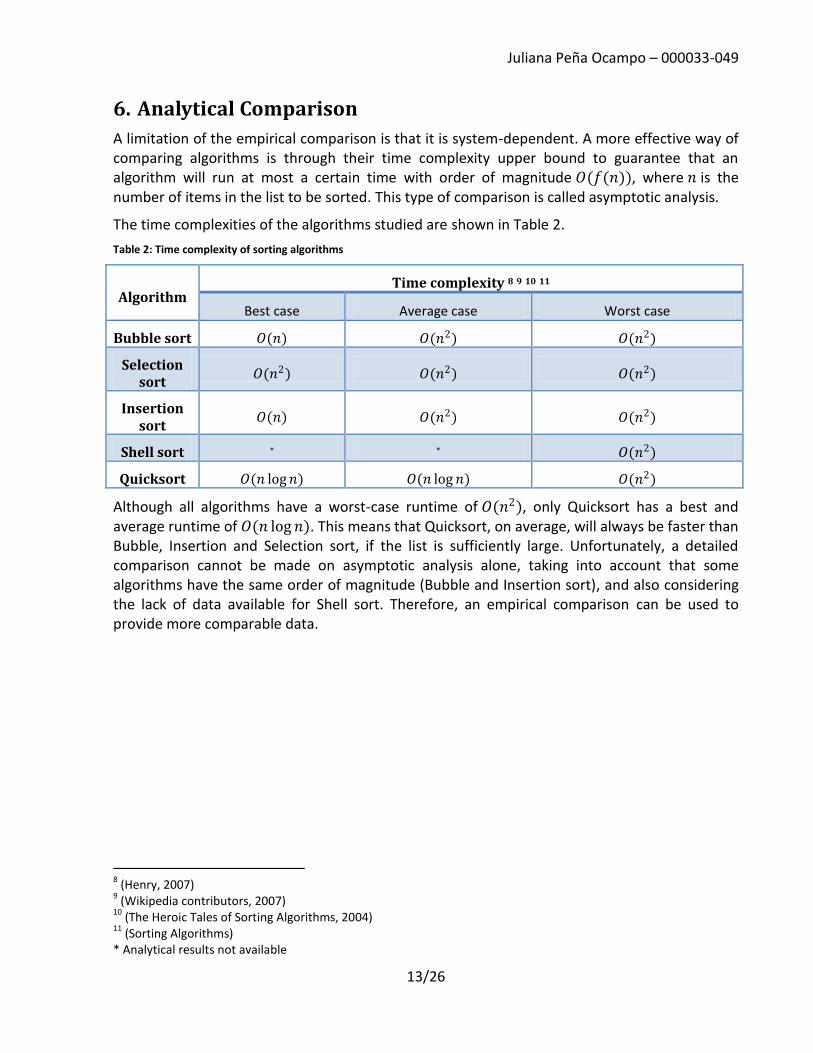
The time complexities of the algorithms studied are shown in Table 2.

Table 2: Time complexity of sorting algorithms

Algorithm Time complexity 8 9 10 11

Best case Average case Worst case

Bubble sort 𝑂(𝑛) 𝑂(𝑛2) 𝑂(𝑛2)

Selection sort

𝑂(𝑛2) 𝑂(𝑛2) 𝑂(𝑛2)

Insertion sort

𝑂(𝑛) 𝑂(𝑛2) 𝑂(𝑛2)

Shell sort * * 𝑂(𝑛2)

Quicksort 𝑂(𝑛 log𝑛) 𝑂(𝑛 log𝑛) 𝑂(𝑛2)

Although all algorithms have a worst-case runtime of 𝑂(𝑛2), only Quicksort has a best and average runtime of 𝑂(𝑛 log𝑛). This means that Quicksort, on average, will always be faster than Bubble, Insertion and Selection sort, if the list is sufficiently large. Unfortunately, a detailed comparison cannot be made on asymptotic analysis alone, taking into account that some algorithms have the same order of magnitude (Bubble and Insertion sort), and also considering the lack of data available for Shell sort. Therefore, an empirical comparison can be used to provide more comparable data.

8 (Henry, 2007)


10 (The Heroic Tales of Sorting Algorithms, 2004)

11 (Sorting Algorithms)

* Analytical results not available


14/26

7. Empirical comparison

7.1. Tests made

The tests were made using the Python script in Appendix A. Each algorithm was run one thousand times on randomly shuffled lists of numbers. The lengths of the lists were 5, 10, 50, 100, 500, 1000, and 5000 for all algorithms and 10000 and 50000 for only Shell sort and Quicksort, due to the enormous amount of time the process would take otherwise. The timing was recorded using the Python timeit module.

The code was run on standard Python 2.5 under Windows Vista, with a 3GHz Pentium 4 (single core with Hyper-Threading) processor and 1GB of RAM.

The raw results were recorded by the script in a file called out.txt. The contents of this file are available in Appendix B. These raw results were tabulated, averaged, and graphed.


15/26

7.2. Results

7.2.1. Total Results

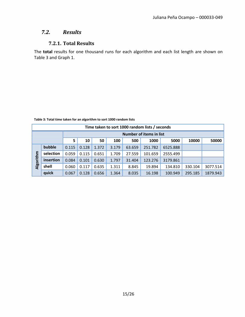
The total results for one thousand runs for each algorithm and each list length are shown on Table 3 and Graph 1.

Table 3: Total time taken for an algorithm to sort 1000 random lists

Time taken to sort 1000 random lists / seconds

Number of items in list

5 10 50 100 500 1000 5000 10000 50000

Alg

ori

thm

bubble 0.115 0.128 1.372 3.179 63.659 251.782 6525.888

selection 0.059 0.115 0.651 1.709 27.559 101.659 2555.499

insertion 0.084 0.101 0.630 1.797 31.404 123.276 3179.861

shell 0.060 0.117 0.635 1.311 8.845 19.894 134.810 330.104 3077.514

quick 0.067 0.128 0.656 1.364 8.035 16.198 100.949 295.185 1879.943


16/26

Graph 1: Total time taken for an algorithm to sort 1000 random lists

0.010

0.100

1.000

10.000

100.000

1000.000

10000.000

100000.000

1000000.000

1 10 100 1000 10000 100000

Tim

e t

ake

n t

o s

ort

10

00

ran

do

m li

sts

/ se

con

ds


bubble

selection

insertion

shell

quick


17/26

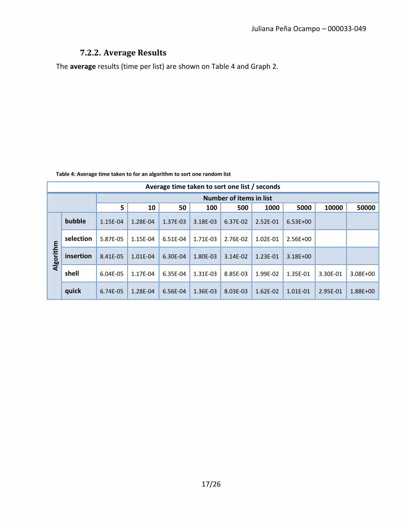
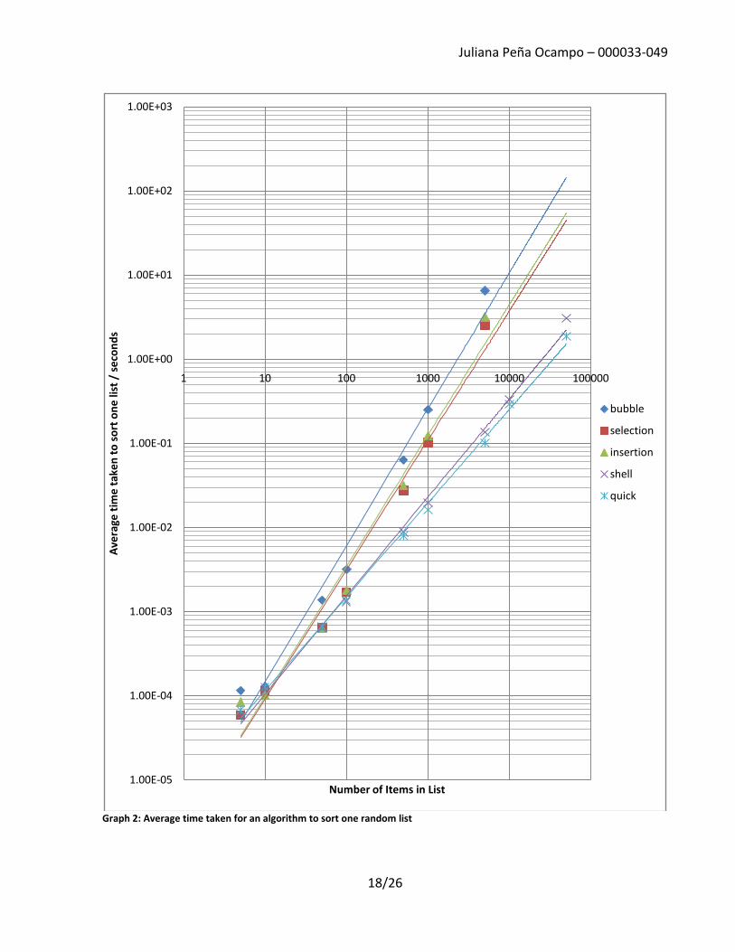
7.2.2. Average Results

The average results (time per list) are shown on Table 4 and Graph 2.

Table 4: Average time taken to for an algorithm to sort one random list

Average time taken to sort one list / seconds


5 10 50 100 500 1000 5000 10000 50000

Alg

ori

thm

bubble 1.15E-04 1.28E-04 1.37E-03 3.18E-03 6.37E-02 2.52E-01 6.53E+00

selection 5.87E-05 1.15E-04 6.51E-04 1.71E-03 2.76E-02 1.02E-01 2.56E+00

insertion 8.41E-05 1.01E-04 6.30E-04 1.80E-03 3.14E-02 1.23E-01 3.18E+00

shell 6.04E-05 1.17E-04 6.35E-04 1.31E-03 8.85E-03 1.99E-02 1.35E-01 3.30E-01 3.08E+00

quick 6.74E-05 1.28E-04 6.56E-04 1.36E-03 8.03E-03 1.62E-02 1.01E-01 2.95E-01 1.88E+00


18/26

Graph 2: Average time taken for an algorithm to sort one random list

1.00E-05

1.00E-04

1.00E-03

1.00E-02

1.00E-01

1.00E+00

1.00E+01

1.00E+02

1.00E+03

1 10 100 1000 10000 100000

Ave

rage

tim

e t

ake

n t

o s

ort

on

e li

st /

se

con

ds

Number of Items in List

bubble

selection

insertion

shell

quick


19/26

8. Conclusions and Evaluation

8.1. Conclusions

The empirical data obtained reveals that the speed of each algorithm, from slowest to fastest for a sufficiently large list, ranks as follows:

1. Quicksort 2. Shell sort 3. Selection sort 4. Insertion sort 5. Bubble sort

There is a large difference in the time taken to sort very large lists between the fastest two and the slowest three. This is due to the efficiency Quicksort and Shell sort have over the others when the list sorted is sufficiently large. Also, the results show that for a very small list size, only selection sort and insertion sort are faster than Quick and Shell sort, and by a very small amount. It should also be noted that Quicksort is eventually faster than Shell sort, though it is slower for small lists.

In a practical sense, the difference between the speeds of Quicksort and Shell sort are not noticeable unless the list is very large (has over 1000 items). For very small lists, the difference between all the algorithms is too small to be noticeable. However, Shell sort is much less system-intensive than Quicksort because it is not recursive.

Considering all this, the application of the results in this investigation in everyday computing could lead as follows:

For lists expected to be less than 1000 items, Shell sort is the optimal algorithm. It is in-place, non-recursive, and fast, making it sufficiently powerful for everyday computing.

For lists expected to be very large (for example, the articles in a news website’s archive, or the names in a phonebook) Quicksort should be used because, despite its larger use of space resources, it is significantly faster than any other of the algorithms in this investigation when the array is sufficiently large.


20/26

8.2. Evaluation

8.2.1. Limitations of an empirical comparison

Although an effective way to compare how different algorithms perform on a system, the main disadvantage of empirical data is that it is entirely dependent on the computer it has been obtained on. Very different results can arise from running algorithms on systems as dissimilar as a mainframe and a cell phone. Different variables, such as memory, processor, operating system, and currently running programs can affect the runtime of the algorithms. This was kept constant in this investigation by always running all the algorithms on the same system. Nonetheless, this type of study does not come to any system-independent conclusions.

Similarly to the previous statement, programming language and compiler/interpreter used can also affect the speed of programs. This research used Python, but if the algorithms were implemented in a language such as C, the result would have probably been much faster sorting, due to C’s compiled nature over Python’s interpreted approach. Also, if the language the algorithms were implemented with was particularly efficient at, for example, recursion, Quicksort might have gotten a much smaller runtime. This leads to another limitation of this sort of investigation: it does not conclude anything about code-independent algorithms.

The solution to this drawback would be to use a system-independent method of analyzing algorithms. This is explored in section 6, by using asymptotic analysis. By obtaining relevant data from the analysis of algorithms, a concrete comparison regarding their speed can be used to obtain system and programming language independent results. The complexity of this method, however, is beyond the scope of this extended essay.

8.2.2. Limitation of a runtime-based comparison

Although speed of algorithms is a very important factor, it is not the only factor that must be taken into account when comparing algorithms. There are many others that can be taken into account, such as memory usage, CPU usage, algorithm correctness, code reusability, et cetera. A comparison of these and other factors could lead to determine which algorithm, as a whole, is most efficient.

8.2.3. Limitations of a comparison based on random arrays

The algorithms in this investigation sorted purely random arrays generated by shuffling sequences of numbers using Python's built-in randint method (see Appendix A, shuffle method). This analysis may show the expected time needed for an algorithm to sort a random list; however, most of the time lists in computing are not entirely random. Usually, long lists are not created from scratch, but rather they are continuously being created by adding items to it. Therefore, most unsorted lists in computing will actually be mostly sorted. This kind of list, however, was not explicitly studied in this investigation, though it is possible that it was randomly generated by the shuffle method. Apart from only random and mostly sorted lists, arrays sorted in reverse order and arrays with duplicate elements could also have been investigated to lead to more thorough conclusions on the best algorithm.


21/26

8.2.4. Exploration of other types of algorithms

A possible improvement to this research would be to compare other types of sorting algorithms. All those presented in this investigation are comparison-based, and, with the exception of Quicksort, simple (make no use of recursion, external functions, or special data types) algorithms. Other possible algorithms to study could include Merge sort (which uses a helper function), Heap sort (which uses a special data type, called a heap), and Radix sort (which is not comparison-based and has a linear time complexity).


22/26

Bibliography

Astrachan, O. (2003, February). Duke University Computer Science Department. Retrieved Octorber 2, 2007, from Bubble Sort: An Archaeological Algorithmic Analysis: http://www.cs.duke.edu/~ola/papers/bubble.pdf

Baecker, R. (2006, July 19). Sorting out Sorting. Retrieved February 16, 2008, from YouTube: http://www.youtube.com/watch?v=F3oKjPT5Khg ; http://www.youtube.com/watch?v=YvTW7341kpA ; http://www.youtube.com/watch?v=plAi7kcqMNU ; http://www.youtube.com/watch?v=gtdfW3TbeYY ; http://www.youtube.com/watch?v=wdcoRfS8edM

Cormen, T., Leiserson, C., & Rivest, R. (2000). Introduction to Algorithms. Cambridge, MA: The MIT Press.

Henry, R. (2007, February 25). Sorting Algorithms Demonstration in Java. Retrieved January 19, 2008, from http://home.westman.wave.ca/~rhenry/sort/

Joyannes Aguilar, L. (2003). Fundamentos de programación: Algoritmos, Estructuras de datos, y Objetos. Madrid: McGraw-Hill/Interamericana de España, S.A.U.

Lamont, M. (2003, December 18). Sorting Algorithms. Retrieved October 10, 2007, from WKU-Linux: http://linux.wku.edu/~lamonml/algor/sort/

Lang, H. W., & Flensburg, F. H. (2007, August 31). Sequential and parallel sorting algorithms. Retrieved October 10, 2007, from http://www.inf.fh-flensburg.de/lang/algorithmen/sortieren/algoen.htm

Lee, R., Tseng, S., Chang, R., & Tsai, Y. (2007). Introducción al diseño y análisis de algoritmos. Mexico City: McGraw-Hill Interamericana.

Sorting Algorithms. (n.d.). Retrieved January 19, 2008, from http://www.cs.wm.edu/~wm/CS303/ln7.pdf

Stedfast, J. (2007, March 3). Algorithms. Retrieved October 10, 2007, from A Moment of Zen: http://jeffreystedfast.blogspot.com/search/label/algorithms

The Heroic Tales of Sorting Algorithms. (2004, April 26). Retrieved January 19, 2008, from http://tanksoftware.com/tutes/uni/sorting.html

Wikipedia contributors. (2007, October 7). Sorting algorithm. (Wikipedia, The Free Encyclopedia) Retrieved October 10, 2007, from http://en.wikipedia.org/w/index.php?title=Sorting_algorithm&oldid=162949511


23/26

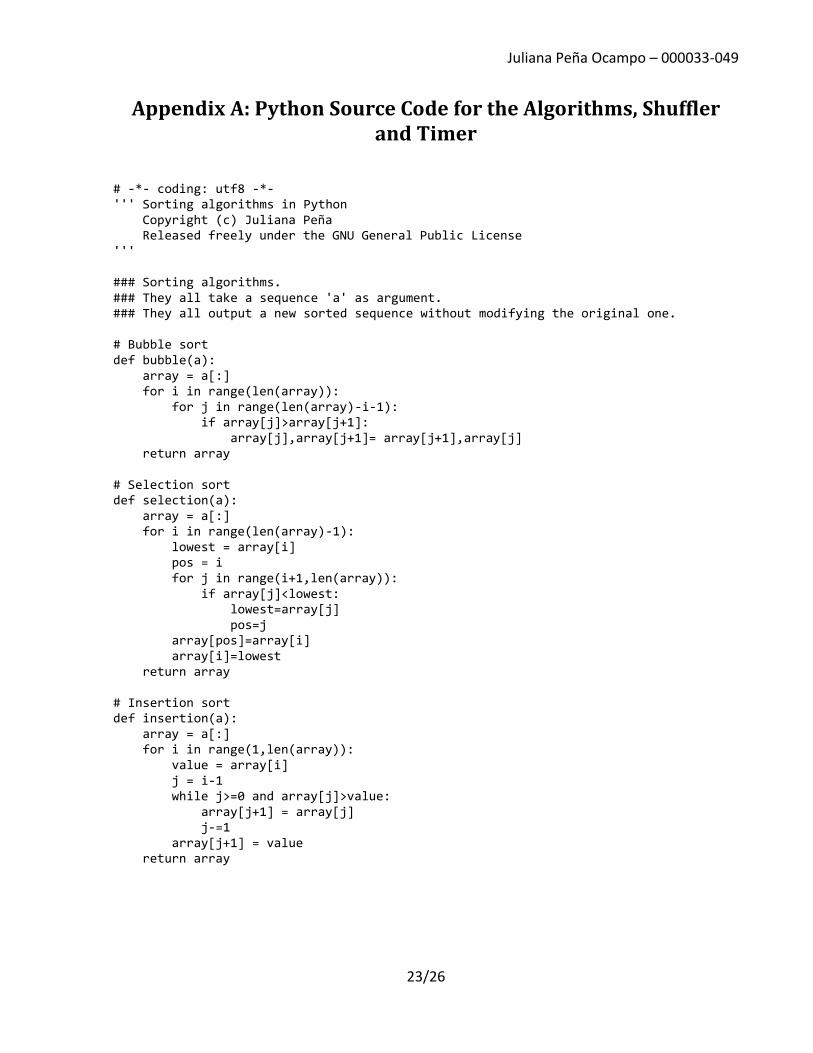
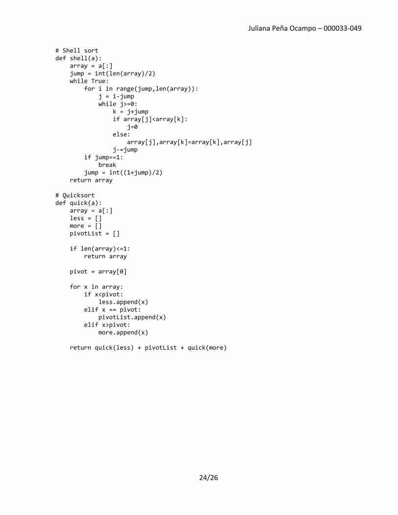
Appendix A: Python Source Code for the Algorithms, Shuffler and Timer

# -*- coding: utf8 -*- ''' Sorting algorithms in Python Copyright (c) Juliana Peña Released freely under the GNU General Public License ''' ### Sorting algorithms. ### They all take a sequence 'a' as argument. ### They all output a new sorted sequence without modifying the original one. # Bubble sort def bubble(a): array = a[:] for i in range(len(array)): for j in range(len(array)-i-1): if array[j]>array[j+1]: array[j],array[j+1]= array[j+1],array[j] return array # Selection sort def selection(a): array = a[:] for i in range(len(array)-1): lowest = array[i] pos = i for j in range(i+1,len(array)): if array[j]<lowest: lowest=array[j] pos=j array[pos]=array[i] array[i]=lowest return array # Insertion sort def insertion(a): array = a[:] for i in range(1,len(array)): value = array[i] j = i-1 while j>=0 and array[j]>value: array[j+1] = array[j] j-=1 array[j+1] = value return array


24/26

# Shell sort def shell(a): array = a[:] jump = int(len(array)/2) while True: for i in range(jump,len(array)): j = i-jump while j>=0: k = j+jump if array[j]<array[k]: j=0 else: array[j],array[k]=array[k],array[j] j-=jump if jump==1: break jump = int((1+jump)/2) return array # Quicksort def quick(a): array = a[:] less = [] more = [] pivotList = [] if len(array)<=1: return array pivot = array[0] for x in array: if x<pivot: less.append(x) elif x == pivot: pivotList.append(x) elif x>pivot: more.append(x) return quick(less) + pivotList + quick(more)


25/26

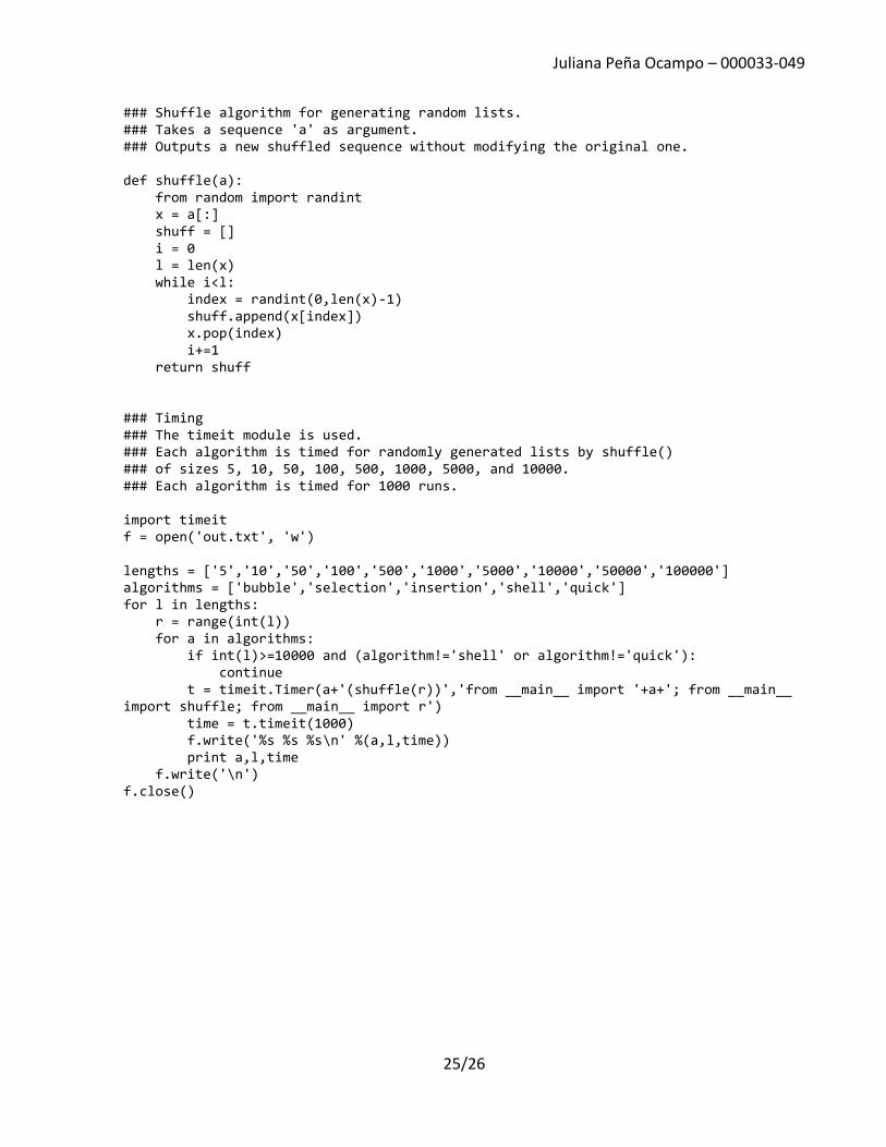
### Shuffle algorithm for generating random lists. ### Takes a sequence 'a' as argument. ### Outputs a new shuffled sequence without modifying the original one. def shuffle(a): from random import randint x = a[:] shuff = [] i = 0 l = len(x) while i<l: index = randint(0,len(x)-1) shuff.append(x[index]) x.pop(index) i+=1 return shuff ### Timing ### The timeit module is used. ### Each algorithm is timed for randomly generated lists by shuffle() ### of sizes 5, 10, 50, 100, 500, 1000, 5000, and 10000. ### Each algorithm is timed for 1000 runs. import timeit f = open('out.txt', 'w') lengths = ['5','10','50','100','500','1000','5000','10000','50000','100000'] algorithms = ['bubble','selection','insertion','shell','quick'] for l in lengths: r = range(int(l)) for a in algorithms: if int(l)>=10000 and (algorithm!='shell' or algorithm!='quick'): continue t = timeit.Timer(a+'(shuffle(r))','from __main__ import '+a+'; from __main__ import shuffle; from __main__ import r') time = t.timeit(1000) f.write('%s %s %s\n' %(a,l,time)) print a,l,time f.write('\n') f.close()


26/26

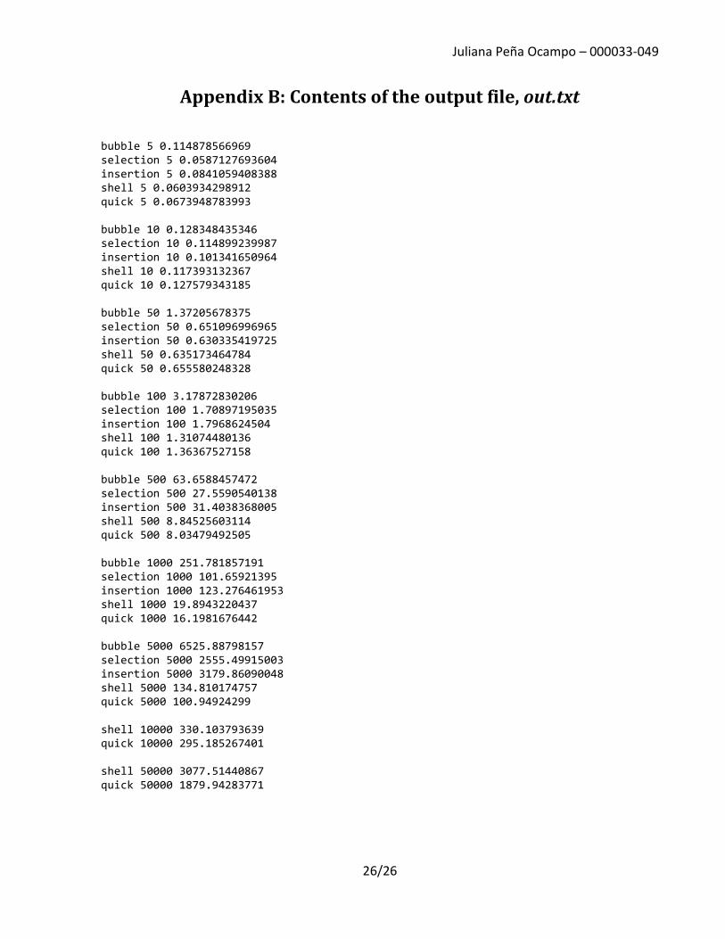
Appendix B: Contents of the output file, out.txt

bubble 5 0.114878566969 selection 5 0.0587127693604 insertion 5 0.0841059408388 shell 5 0.0603934298912 quick 5 0.0673948783993 bubble 10 0.128348435346 selection 10 0.114899239987 insertion 10 0.101341650964 shell 10 0.117393132367 quick 10 0.127579343185 bubble 50 1.37205678375 selection 50 0.651096996965 insertion 50 0.630335419725 shell 50 0.635173464784 quick 50 0.655580248328 bubble 100 3.17872830206 selection 100 1.70897195035 insertion 100 1.7968624504 shell 100 1.31074480136 quick 100 1.36367527158 bubble 500 63.6588457472 selection 500 27.5590540138 insertion 500 31.4038368005 shell 500 8.84525603114 quick 500 8.03479492505 bubble 1000 251.781857191 selection 1000 101.65921395 insertion 1000 123.276461953 shell 1000 19.8943220437 quick 1000 16.1981676442 bubble 5000 6525.88798157 selection 5000 2555.49915003 insertion 5000 3179.86090048 shell 5000 134.810174757 quick 5000 100.94924299 shell 10000 330.103793639 quick 10000 295.185267401 shell 50000 3077.51440867 quick 50000 1879.94283771

An empirical comparison of the runtime of five sorting ...uploads.julianapena.com/ib-ee.pdf · An...

Documents

Transcript of An empirical comparison of the runtime of five sorting ...uploads.julianapena.com/ib-ee.pdf · An...