- 1 -

AN EMPIRICAL ANALYSIS OF FINANCIAL DEEPENING AND ECONOMIC

GROWTH IN NIGERIA: (1986 – 2010)

BY

ONYEMACHI CHUKWUKA

DEPARTMENT OF ECONOMICS,

AHMADU BELLO UNIVESITY, ZARIA, NIGERIA

MAY 2012

- 2 -

AN EMPIRICAL ANALYSIS OF FINANCIAL DEEPENING AND ECONOMIC GROWTH IN NIEGRIA (1986-2010)

BY

ONYEMACHI CHUKWUKA

M.SC/SOC.SCI/01842/2008/2009

A THESIS SUBMITTED TO THE POSTGRADUATE SCHOOL

IN AHMADU BELLO UNIVERSITY, ZARIA, NIGERIA

IN PARTIAL FULFILMENT FOR THE AWARD OF MASTERS OF SCIENCE IN

ECONOMICS (M.SC)

DEPARTMENT OF ECONOMICS, AHMADU BELLO UNIVESITY,

ZARIA, NIGERIA.

MAY 2012

- 3 -

DECLARATION I hereby declare that the thesis titled, “AN EMPIRICAL ANALYSIS OF FINANCIAL

DEEPENING AND ECONOMIC GROWTH IN NIGERIA (1986-2010)” is the result of a

research work carried out by, ONYEMACHI CHUKWUKA in the Department of Economics

under the supervision of PROF. (MRS) P. S. AKU and DR NJIFORTI PETER.

The information derived from the literature has been dully acknowledged in the text and a list

of references provided. No part of this thesis was presented previously for another degree or

diploma at any university.

…………………….. …………………….. ………………...........

Name of Student Signature Date

- 4 -

CERTFICATION This is to certify that the thesis titled, “AN EMPIRICAL ANALYSIS OF FINANCIAL

DEEPENING AND ECONOMIC GROWTH IN NIGERIA (1986-2010)” written by

Onyemachi Chukwuka meets the requirements and regulations governing the award of

Masters of Science Degree (Economics) in the Department of Economics of Ahmadu Bello

University, Zaria and is hereby approved for its contribution to knowledge and literary

presentations.

…………………………………………… ……………………………

PROF (MRS.) P. S. AKU DATE CHAIRMAN, SUPERVISORY COMMITTEE

………………………………………… ……………………………..

DR. PETER NJIFOTI DATE MEMBER, SUPERVISORY COMMITTEE

………………………………………. …………………………….. DR. M. M. USMAN DATE HEAD OF DEPARTMENT

……………………………………. ……………………………. PROFESSOR A. A JOSHUA DATE DEAN, POST GRADUATE SCHOOL

- 5 -

DEDICATION

This thesis is dedicated to God Almighty. It is dedicated to my parents Mr.

Christopher U. Onyemachi and Mrs. Justina N. Onyemachi; to my siblings, Adanma,

Chinyere, Udobi, Ibeabuchi, and Ozioma and fiancée Uzonwanne Okezie.

- 6 -

ACKNOWLEDGEMENT

All Glory be to God, for His steadfast love, amazing grace, goodness and mercy upon my

life. May His name alone be praised.

My gratitude goes to my supervisors, PROF (MRS.) P. S AKU and DR. NJIFORTI PETER.

I am highly indebted to them for their contributions and valuable advice, constructive

criticisms, concrete suggestions, relentless effort and cooperation towards the success of this

that enhanced the quality of this work.

My heartfelt gratitude goes to my parents Mr. and Mrs C. U. Onyemachi for their love, moral

and financial support, whose hard work and disciplined life-style inspired me to choose the

path of headwork and discipline as a way of life and for the achievement of greatness. You

are the best. To my siblings, Adanma, Chinyere, Udobi, Ibeabuchi and Ozioma, who have

always been there for me, I say thank you. I love you all. I am also obliged to my sweet heart,

Uzonwanne Okezie, my fiancée for her love and support.

I am indebted to Louis Sevitenyi Nkwatoh for his, advice, support and time, I say thank you.

My sincere appreciation goes to all my friends, Toyin, Bash, Kate, Leo, Philip, Majeed, Paul,

Helen, Safe, Aliyu, Iyabo, Mercy, Solomon and all my course mates, thanks for your

companionship, encouragement and cooperation.

- 7 -

ABSTRACT

Economists have long recognized that the financial system plays a decisive role in the

process of economic development (Stiglitz, 1998), some have argued that financial

intermediaries mobilize, pool and channel domestic savings into productive capital, and by

doing so they contribute to economic growth (supply leading), while others argue, that

financial development is a consequence, and not a cause of economic growth. In this view,

economic growth increases demand for sophisticated financial instruments, which in turn

leads to growth in the financial sector (demand following). This study examines the causal

relationship between financial deepening and economic growth in Nigeria for the period

1986 to 2010 using the Vector Auto Regressive model. From the results of the analysis, we

found out that; financial deepening does not impact or influence economic growth in the

short run. However, in the long run there is a significant effect of financial deepening on

economic growth, lending credence to the supply leading hypothesis that financial deepening

causes economic growth. It was also observed that GDP had a positive and significant

impact on Deposit Money Bank Asset, Money supply and private sector credit, thereby laying

credence to the demand following hypothesis. It was recommended that monetary authorities

should continue with the policy reforms to consolidate the emerging confidence in the

financial system.

- 8 -

CONTENTS

Title Page ……………………………………………………………………………... i

Declaration.………………………………………………………………………….....ii

Certification ………………………………………………….……………………..... iii

Declaration………………………………………………………………………….… iv

Acknowledgements ………………………….……………………………………….. v

Abstract ……………………………………………………………………………..... vi

CHAPTER ONE: INTRODUCTION

1.1 Background to study ……………………………….……………………………...... 1

1.2 Problem Statement ……………………………………...……….………………...... 4

1.3 Objectives of Study …………………………………………………….....………… 6

1.4 Research Hypothesis.................................................................................................... 6

1.4 Justification of Study …………………………………………………….....……….. 7

1.5 Scope of the Study………………………..…………………………………......…… 7

1.6 Organisation of the Study …………………………………………………................ 7

CHAPTER TWO: LITERATURE REVIEW

2.1 Conceptual framework ………………… ……………….…….……………….…. 8

2.1.1 Financial Deepening ……………………………........................................…. 8

2.1.2 Economic Growth ………………………………………………………….…….9

2.2. The Structure of the Nigerian Financial system ……………….….………….... 10

2.2.1 Money Market …………………….……………………………………....… 11

2.2.2 Capital Market.................................................................................……..... 11

2.2.3 Financial Deepening in Nigeria …………………………………….…..…....... 13

2.3 Theoretical Literature review ……………………………………………………14

2.3.1 The Endogenous Growth Mode …………………………..………..……………15

- 9 -

2.3.2 Harrod – Domar Model …………………………. ………………..……………. 17

2.3.3 Supply – Leading Hypothesis …..…………………………………...………….. 20

2.3.4 Demand – Pulling Hypothesis …………..………………………..……..……… 21

2.4 Stages of Financial Deepening ………………………………...…………….…….. 22

2.5 Impact of Financial Deepening on Economic Growth ………..…………….…. 26

2.6 Empirical Literature Review …………………………….……………………....... 28

CHAPTER THREE: RESEARCH METHODOLOGY

3.1 Introduction ……………………………………………..……………………….... 34

3.2 Source of Data ................................................................................................ 34

3.3 Analytical Technique....................................................................................... 34

3.4 Model Specification ……………………………………………………………...... 35

3.5 Estimation Techniques……………………………………………………………... 37

3.5.1 Unit Root ......................................................................................................37

3.5.2 Granger Causality Test .................................................................................. 38

3.5.3 Impulse Response .......................................................................................... 39

3.5.4 Variance Decomposition .................................................................................40

3.3 A Priori Expectations………………………..……..…………….……..……….......40

CHAPTER FOUR: DATA ANALYSIS AND PRESENTATION OF RESULTS

4.1 Introduction ………………………………………………………………………….41

4.2 Trend, Structure and Growth of Financial Deepening Nigeria …………………….41

4.3 Empirical Analysis ……………….………….......…………….…………………….46

4.4 Analysis of Regression Results ……………………………………………………...57

- 10 -

CHAPTER FIVE: Summary, Conclusion and Recommendations

5.1 Summary …………………………………………………………………….…... 59

5.2 Major Findings …………………………………………………………………… 60

5.3 Conclusion ……………………………………………………………………….. 61

5.4 Recommendations ……………………………………………………..…………… 62

5.5 Direction of Research ………………………………………………………………. 62

REFERENCES …………………………………………….……..…………………….. 63

APPENDICES ………………………………………………......……………………… 70

LIST OF TABLES

Table 2.1: Financial development indicators in Nigeria (1970 – 2008) ……………….. 13

Table4.1: Trend in selected monetary and economic aggregates ……………………… 42

Table 4.2: Gross domestic product and performance of the Nigerian capital market from

1981-2008 ……………………………………………………………………………….44

Table 4.3: Selected Financial Deepening Indicators …………………………………….45

Table 4.4: Unit Root Test ………………………………………………………………. 46

Table 4.5: Granger causality test ……………………………………………………….. 48

Table 4.6: Lag Length Selection Criteria ………………………………………………. 49

Table 4.7: Variance Decomposition of GDP …………………………………………… 56

Table 4.8: Standard errors & t-statistics ………………………………………………… 58

LIST OF FIGURES Fig 2.1: The Nigerian Financial System ……………………………………………….... 13

Figure 2.2: Channels: Finance and growth model of King and Levine (1993) ……..…. 16

Figure 2.3: Three regions of financial deepening. ………………………………..….. 23

- 11 -

Fig 4.1(a-h): Impulse response functions of GDP to a shock in the explanatory variables 51

Fig 4.2 (a-h): Impulse response functions of the explanatory variables to a shock in GDP 55

- 12 -

CHAPTER ONE

INTRODUCTION

1.1 BACKGROUND TO THE STUDY

Financial deepening implies the ability of financial institutions to effectively mobilize

savings for investment purposes. The growth of domestic savings provides the real structure

for the creation of diversified financial claims. Financial deepening generally entails an

increased ratio of money supply to Gross Domestic Product (Popiel, 1990), Nnanna and

Dogo, 1999) and Nzott, 2004). The sum of all the measures of financial assets gives us the

approximate size of financial deepening. That means that the widest range of such assets as

broad money, liabilities of non-bank financial intermediaries, treasury bills, value of shares in

the stock market, money market funds, etc, will have to be included in the measure of

financial deepening.

Indicators of financial deepening differ in economies and between the countries. It is

also possible that, different financial markets have different levels of financial deepening, for

example, the countries that have efficient financial systems have higher financial deepening

ratios. The share of assets in GNP of developed countries’ financial markets is greater than

that of the developing countries (Jovanovic, 1990).

The financial system has been acknowledged globally to play a catalytic role in the

economic development of nations (Sanusi, 2009). It plays a key role in the mobilization and

allocations of savings for productive use, provides structures for monetary management, the

basis for managing liquidity in the system. It also assists in the reduction of risks faced by

firms and businesses in their productive processes, improvement of portfolio diversification

and the insulation of the economy from the vicissitudes of international economic changes.

The increasing deepening and expansion of the financial system is expected to lead to

increased variety of financial instruments not only in the banking subsector but also in the

- 13 -

capital market. Greater availability of varieties of financial institutions and instruments is

expected to deepen the financial system. Financial deepening can be measured using several

kinds of indices, a few of these are: the ratio of the growth rate of broad money (M2) to that

of the gross domestic product; ratio of Total banking assets to GDP, Gross Savings in the

economy to GDP as well as Gross Domestic Investment to GDP as well as the Interest Rate

Spread (i.e the difference between lending rate and deposit rate). The more deepened the

financial system the more expanded the level of output and the rate of growth of output are

supposed to be.

Goldsmith (1969) motivated his path breaking study of finance and growth as follows:

“One of the most important problems in the field of finance, if not the single most important

one … is the effect that financial structure and development have on economic growth.”

Economic growth cannot be possible without the combined role of investment, labour and

financial deepening (Ndebbio, 2004). Though Economists have accepted effects of financial

deepening on economic growth, they have not had the same idea about the direction of

causality, which means whether financial development causes economic growth or economic

growth causes financial development. For instance, Hicks (1969), Shaw (1973) and

Schumpeter (1912) support that financial development causes economic growth, that is,

financial deepening is a necessary pre-condition for economic growth. This hypothesis is

usually labeled “supply leading” since it postulates that the presence of efficient financial

markets increases the supply of financial services in advance of the demand for them in the

real sector of the economy. In contrast to this opinion, Robinson (1952) and Patrick (1966)

discusses that in the existence of same type of financial regulations, economic growth creates

a demand, and financial system gives an automatic response to this demand which causes

financial system development. They argue that financial deepening is merely a by-product or

an outcome of growth in the real side of the economy. This is called the “demand-following”

- 14 -

hypothesis since financial markets develop and progress following the increased demand for

their services from the growing real economy.

Theoretically, financial development creates enabling conditions for growth through

either a supply leading (financial development spurs growth) or a demand following (growth

generates demand for financial products) channel, (Smith, 2007). A large body of empirical

research supports the view that development of the financial system contributes to economic

growth (Rajan and Zingales, 2003).

The reforms in the financial system in Nigeria which heightened with the 1986

deregulation, affected the level of financial deepening of the country and the level relevance

of the financial system to economic development (Nnanna and Dogo, 1998). However, the

rapid globalization of the financial markets since then and the increased level of integration

of the Nigerian financial system to the global system have generated interest on the level of

financial deepening that has occurred.

Nigeria has experienced growth in the financial sector and consequently increases in

financial deepening over time. Growth in financial outlet, development in the money and

capital market increases in stocks, and activities in the capital market, increases bank

branches, rapid use of credit and debit cards, increasing use of payment technologies like

ATM machines(Automatic Teller Machine Technology) and electronic transfer of deposits,

expanding Internet banking services, e-banking, and increase in total deposits, (Luis, 2009).

Growth in financial sector should translate into the growth of the economy, because growth

in the financial sector will make available funds for investment.

In the capital market, market capitalization is the most widely used indicator in

assessing the size of a capital market to an economy. Before 1988, the total market

capitalization was less than N10 billion from 1988 to 1994, it hovered between N10 billion to

N57 billion. In 2003, it was N1,3593 trillion, N2.1125 trillion in 2004 and N5.12 trillion in

- 15 -

2006.The market capitalization recorded the highest value of N13.2294 trillion in 2007. But

this fell to N9.562 trillion in 2008 due to the global financial meltdown. The percentage

market capitalization compared to the economy’s Gross Domestic Product (GDP) helps to

assess the size of the stock market. In 1981, this was 10.5%, but fell to 7.4% in 1994. It rose

again to 9.3% in 1995, 10.6% in 1996; 18.9% in 2003, 25.6% in 2004 and 27.4% in 2005.

The question is whether the development in the financial sector, which has led to

financial deepening, has been able to bring about anticipated growth, considering the fact that

Nigeria still experiences high level of unemployment, inflation rates are still high, lack of

credit for investment, the deposit and lending rates are still very wide apart, there is wide

disparity between the lending and deposit rates. Therefore, this study examines the extent to

which financial deepening has impacted on economic growth in Nigeria.

1.2 STATEMENT OF PROBLEM

The relevance of the financial system to economic growth is not clear-cut. The

direction of causality between financial deepening and growth has always been a

controversial issue. There are two main opposing hypotheses which are testable: the ‘supply-

leading’ hypothesis versus the ‘demand-following’ hypothesis. Supply-leading emphasizes

financial deepening as an important prerequisite for growth. The supply-leading hypothesis

suggests that financial deepening fuels growth. The existence and development of the financial

markets brings about a higher level of saving and investment and enhance the efficiency of

capital accumulation, (Hicks 1969, Levine 1993, Diego 2003). Demand-following posits

that financial deepening follows growth; development of the financial markets is merely a

lagged response to economic growth. This implies that any early efforts to develop financial

markets might lead to a waste of resources which could be allocated to more useful purposes in

the early stages of growth. As the economy advances, this triggers an increased demand for

- 16 -

more financial services and thus leads to greater financial development, ( Robinson 1952,

Lucas 1988, Favara 2003).

Since 1986, the monetary authorities in Nigeria have adopted various measures

aimed at deepening the financial system and reducing the level of financial repression in the

system. The reform of the financial structure led to changes in Nigeria’s financial sector in an

effort to foster competition, strengthen the supervisory role of the regulatory authority and

streamline the relationship between the public and financial sectors of the economy. Many

new financial instruments/assets and techniques have been developed and existing ones have

been modified, the financial markets have been adapted to meet new demands and new

circumstances. All these have been aimed at deepening the financial system. But how has all

these impacted on economic growth in Nigeria.

This research will examine the causal relationship that exists between finance and

growth within the Nigerian economy, is it supply leading or demand following in nature?

1.3 OBJECTIVES OF THE STUDY

The main objective of the study is to examine empirically the extent of financial

deepening in Nigeria, and its impact on the Nigerian economy since the onset of financial

reforms in 1986 up to 2008.

The specific objectives of the study include:

i. To examine the structure and growth of financial deepening in Nigeria.

ii. To analyze the impact of financial deepening on economic growth in Nigeria

iii. To make policy recommendations

- 17 -

1.4 RESEARCH HYPOTHESIS

The research will test one main hypothesis which is as follows:

H1: B1=O Financial deepening has no significant effect on economic growth in Nigeria.

H1: B1 ≠ O Financial deepening has significant effect on economic growth in Nigeria.

1.5 JUSTIFICATION

Although most studies have found that financial development contributes to economic

growth, example McKinnon (1973), Goldsmith (1969), and Levine (1993), they have not

ended the debate on the direction of causality between economic growth and financial

development. It is expected that the outcome of this research will shed more light on the role

of financial deepening on economic growth in Nigeria.

If the development of financial system affects economic growth positively, large

financial deepening rate will make economic growth increase. When this rate is small, due to

weak financial deepening, economic growth will not reach the required level (Greenwood,

1990). Thus, how economic growth is affected by financial development or financial system

is an important point for discussion.

This study contributes to knowledge by investigating empirically the causal relationship

between financial deepening and economic growth in Nigeria using the vector autoregressive

model.

1.6 SCOPE AND LIMITATION

The study covers the period 1986 to 2010. This period however, is considered by the

study wide enough to permit a logical deduction that can influence policy decisions in the

financial sector development. The summing up of financial assets to represent a broad

measure of financial deepening is not a problem, but the availability of data for some of them

is.

- 18 -

1.7 ORGANISATION OF THE STUDY

This research work is structured into five chapters. Chapter One consists of our discussion so

far, which covers the general introduction of the study, statement of problem, objectives of

the study, justification, hypothesis methodology, scope and limitation, and organization of

chapters. Chapter two presents the conceptual framework, theoretical and empirical literature

review, while chapter three presents the methodology; chapter four presents the data analysis

and interpretation. Finally, summary of findings, conclusion and recommendation are

contained in chapter five.

- 19 -

CHAPTER TWO

LITERATURE REVIEW

2.1 CONCEPTUAL FRAMEWORK

2.1.1 FINANCIAL DEEPENING

Financial deepening implies the ability of financial institutions to effectively mobilize

savings for investment purposes. The growth of domestic savings provides the real structure

for the creation of diversified financial claims. Financial deepening generally entails an

increased ratio of money supply to Gross Domestic Product (Popiel, 1990, Nnanna and Dogo,

1999, and Nzotta, 2004).

Financial deepening can be defined as the effort aimed at developing the financial

system that is evident in increased financial instrument/assets in the financial markets –

money and capital markets, leading to the expansion of the real sector of the economy

(Njiforti et’al, 2007). It is the effort of developing countries to achieve growth through

financial intermediation.

The definition of financial deepening in literature reflects the share of money supply in GDP.

The most classic and practical indicator related to financial deepening is the ratio of M2/GDP

which means the share of M1 + all time-related deposits and noninstutional money market

funds to GDP in a certain year (Öçal and Çolak, 1999). Financial deepening is thus measured

by relating monetary and financial aggregates such as M1, M2 and M3 to the Gross Domestic

Product (GDP). M1: Technically defined, is the sum of: the tender that is held outside banks,

travelers checks, checking accounts (but not demand deposits), minus the amount of money

in the Federal Reserve float.

M2: The sum of: M1, savings deposits (this would include money market accounts from

which no checks can be written), and small denomination time deposits

- 20 -

M3: M2 plus the large time deposits.

M1, M2, M3 are all measures of money supply, that is the amount of money in

circulation at a given time. Generally, the types of commercial bank money that tend to be

valued at lower amounts are classified in the narrow category of M1 while the types of

commercial bank money that tend to exist in larger amounts are categorized in M2 and M3,

with M3 having the largest. The terms M1, M2, M3 refer to the monetary aggregates. For

quite some time it was thought that there was a perfect one to one relationship between these

numbers and the rates of inflation. Recently this relationship seems to have broken down,

and the money supply numbers have lost some of their appeal to market participants.

Shaw (1973) explains the changes in system of finance with a term financial

deepening. According to this idea, when financial system has achieved a specific depth,

credits and deposits maturity would become equal.

2.1.2 ECONOMIC GROWTH

Jhingan (2003) defines economic growth as a process whereby the real per capital

income of a country increases over a long period of time. According to him, economic

growth is measured by the increase in the amount of goods and services produced in a

country. Economic growth occurs when an economy’s productive capacity increases which,

in turn, is used to produce more goods and services.

Economic growth is the increase of per capita gross domestic product (GDP) or other

measure of aggregate income. It is often measured as the rate of change in GDP. Economic

growth refers only to the quantity of goods and services produced. The term economic

growth refers to the increase (or growth) of a specific measure such as real national income,

gross domestic product, or per capita income. National income or product is commonly

expressed in terms of a measure of the aggregate value added output of the domestic

- 21 -

economy called gross domestic product, GDP. In other words, GDP is a measure of the value

of all of the goods and services produced in a country in a year. GDP can be calculated as the

value of the output produced either in a country or equivalently as the total income, in the

form of wages, rents, interests, and profits, earned in a country. Thus, GDP is also known as

output or national income.

2.2 THE STRUCTURE OF THE NIGERIAN FINANCIAL SYSTEM

A financial system is a conglomerate of various markets, instruments, operators and

institutions that interact within an economy to provide financial services such as resources

mobilization and allocation, financial intermediation and facilitation of foreign exchange

transaction to exchange foreign trade.

As mentioned earlier, the Nigerian financial system can be broadly subdivided into 2,

namely: the informal and the formal. The informal sector comprises the local money lenders,

the thrifts and savings associations etc. This component is poorly developed, limited in reach,

and not integrated into the formal financial system. Its exact size and effect on the economy

remain unknown and a matter of speculation. The formal financial system on the other hand,

can be subdivided into the money market and capital market and these comprise the banks

and non-bank financial institutions.

2.2.1 THE MONEY MARKET

The money market segment of the financial system constitutes the hub of the financial

system. Its major function is to facilitate the raising of short-term funds from the surplus

sectors to the deficit sectors of the economy and comprises the discount houses, commercial

and special purpose banks like the Community banks. They deal in short term credit

- 22 -

instruments of high quality, such as treasury bills, treasury certificates, call money,

commercial paper and so on.

Commercial banks perform three major functions, namely, acceptance of deposits,

granting of loans, and the operation of the payment and settlement mechanism. In terms of

flow of funds, the banking system, clearly dominates and has an important impact on the

level of economic development. The first commercial bank was established in 1894, and is

the forebear of the present day First Bank of Nigeria PLC. Since the government commenced

the active deregulation of the economy in 1986, the commercial banking sector has continued

to witness rapid growth, especially in terms of the number of institutions and product

innovations in the market. With the bank consolidation of 2005 and bank reforms, Nigeria

has a total of twenty four commercial banks with over 3000 branches nationwide (Ndebibo,

2010)

Discount houses these are non-bank financial institutions that mobilize funds for

investment in securities according to the liquidity needs of the system. Discount houses were

created to serve as financial intermediaries between the CBN, licensed banks and other

financial institutions.

2.2.2 THE CAPITAL MARKET

The Nigerian Capital Market is a channel for mobilization and utilization of long-term

funds. The instruments traded in the market include government securities, government and

corporate bonds and equity and preference shares (stocks) and mortgage loans. The main

institutions in the market include the Securities and Exchange Commission (SEC), which is at

the apex and serves as the regulatory authority of the market, the Lagos Stock Exchange

(LSE), the issuing houses and the stock broking firms. The capital market is classified into

primary and secondary segments. The Lagos Stock Exchange commenced business in 1961.

- 23 -

The Primary Market is a market for new issues of securities. The mode of offer for the

securities traded in this market includes offer for subscription, rights issues, offer for sale and

private placements.

The Secondary Market is a market for trading in existing securities. This consists of

exchange and over-the-counter markets where securities are bought and sold after their

issuance in the primary market. In a strict sense, it constitutes the stock exchange since it is

the mechanism which gives liquidity to the securities listed on the exchange. Activities in the

secondary market have increased substantially over the years.

The structure of the Nigerian financial system, can be summarized in the chart below,

showing that the financial system is made up of bank and non-bank financial institutions

under different regulatory institutions

2.3 FINANCIAL DEEPENING IN NIGERIA

The financial deepening index of MS2/GDP moved from 35.9 in 1986 down to 24.2 in 1992

and increased to 29.7 by 1994. This declined further to 15.3 by 1997 before rising to 32.0 by

2004. The aggregate moved down to 18.0 by 2005 and up again to 29.7 by 2007. The trends

above clearly show that the financial deepening index did not experience any dramatic

changes during the period. This is despite the various reforms introduced from 1986 which

should have a positive effect on financial deepening in Nigeria (Nnanna and Dogo, 2008).

The ratio of currency outside banks to money supply progressively declined between

1997 and 2007. The ratio moved from 30.4 in 1979 down to 15.2 in 2007. This shows a

higher level of banking habits in the country. The decline had been more pronounced

between 2005 and 2007 following the increased use of Automated Teller Machines and

plastic money in the country (Garba, 2003).

- 24 -

Table 2.1: Financial development indicators in Nigeria (1970 – 2008)

Indicators (%)

Before

reforms

During

reforms

(1970 – 1986) (1987 -2008)

M2/GDP 26.7 22.8

Private sector

credit/GDP 16.8 14.4

Currency outside

bank/M2 23 15.7

Interest rate spread 1.8 10.7

Real interest rate -8.1 -15.5

Gross

Savings/GDP 7.1 12.6

Source: CBN Statement Bulletin 2008

2.3 THEORETICAL LITERATURE REVIEW

Theoretically, financial development creates enabling conditions for growth through

either a supply leading (financial development spurs growth) or a demand following (growth

generates demand for financial products) channel. A large body of empirical research

supports the view that development of the financial system contributes to economic growth

(Rajan and Zingales, 2003). The most influential contributions on the relationship between

finance and growth identify financial development as a crucial precondition of long-run

growth, suggesting that financial liberalization is an important instrument of economic

policy.

- 25 -

2.3.1 THE ENDOGENOUS GROWTH MODEL

Bencivenga and Smith (1991) and Levine (1991) were among the first to propose

endogenous growth models to identify the channels through which financial markets affect

long-run economic growth. With the emergence of the endogenous growth theory, the direct

and indirect influence of financial markets on economic growth has drawn considerable

attention, particularly with regard to sound development strategies.

The endogenous growth models show that economic growth performance is related to

financial development, technology and income distribution. The endogenous growth models

focus on the relationship between financial development and long-run economic growth,

emphasizing that productivity growth is most likely to be the channel of transmission from

financial development to economic growth. It is concerned with financial markets, savings,

investments, and growth. The argument is that financial markets will raise savings,

investment and hence the growth rates.

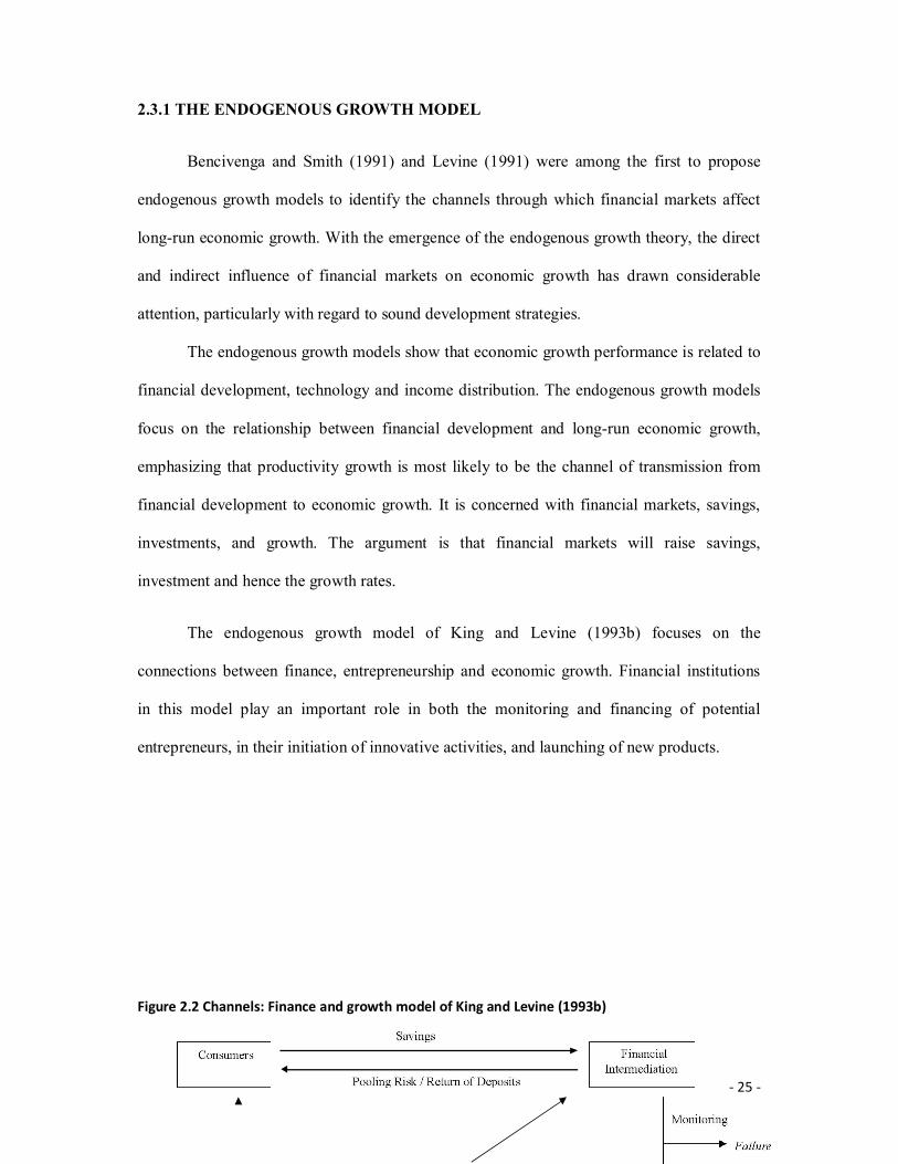
The endogenous growth model of King and Levine (1993b) focuses on the

connections between finance, entrepreneurship and economic growth. Financial institutions

in this model play an important role in both the monitoring and financing of potential

entrepreneurs, in their initiation of innovative activities, and launching of new products.

Figure 2.2 Channels: Finance and growth model of King and Levine (1993b)

- 26 -

Source: King and Levine 1993.

Figure 2.2 displays the channels, through which financial intermediation contributes

to economic growth. Initially, in the entrepreneurial selection procedure, the financial

intermediary monitors the whole set of candidates in the market and picks up potential

entrepreneurs with the ability to manage innovations in the intermediate goods production

technology. Second, the financial intermediary finances the innovative activities. If

entrepreneurs are successful, they will enjoy monopoly profits by producing the unique

intermediate product at a lower cost than their rivals but charging the same price. However,

to produce intermediate goods the successful entrepreneurs need external financing.

The financial intermediary evaluates and finances those entrepreneurs while it can pay

back the consumers (savers) the interest according to its evaluation of the profitability of

those entrepreneurs. Requiring the input of intermediate goods and labor, the production of

final goods is also affected by the innovative success − the productivity increases with the

technological progress. Of course, the aggregate final goods’ production influences the

consumers, who also provide the labor in this model, by affecting their optimal choice of

intertemporal substitution in consumption.

The model identifies the following potential relationships between finance and

growth. First, finance supports innovations and hence increases the productivity which is

positively correlated with growth. Second, efficiency improvements in the financial sector,

such as a decrease in the cost of monitoring, will increase the real rate of return and thus lead

to a higher future growth rate. Third, the model also suggests a reverse channel of causation

where distortions in the innovative sector lower the demand for financial services and retard

financial development.

- 27 -

2.3.2 HARROD-DOMAR GROWTH MODEL

The economic growth models of Harrod and Domar are based on the experiences of

the advanced capitalist economies. They both emphasize the role of investment in economic

growth based on the dual characteristics of investment. Firstly, it creates income and

secondly, it augments the productive capacity of the economy by increasing its capital stock.

The former is regarded as the ‘demand effect’ while the later is the ‘supply effect’ of

investment.

The Harrod - Domar model provides accurate short-term predictions of growth and has

been used extensively in developing countries to determine the required investment rate or

financing gap to be covered in order to achieve a target growth rate. It is based on the

following assumptions.

i. There is an initial full employment equilibrium level of income.

ii. There is the absence of government intervention.

iii. The models operate in a closed economy which has no foreign trade.

iv. The average propensity to save is equal to the marginal propensity to save.

v. There are no lags in adjustments between investment and creation of productive

capacity.

vi. Savings and investment relates to income of the same year.

vii. There is no depreciation of capital goods.

- 28 -

Based on the above assumptions, Domar’s model was built on premise that to maintain

full employment equilibrium level of income, aggregate demand should be equal to aggregate

supply. Thus, we arrive at the fundamental equation of the model.

∆Iα=Iδ………………………………………………… 1

Where I= Investment,

∆I = Changes in Investment,

α = Marginal propensity to save

δ = Net potentials social average productivity of investment (=∆Y/I)

Solving equation (1) by dividing both sides by I and multiplying by α we get:

∆I/I= α δ……………………………………….. 2

This equation shows that to maintain full employment the growth rate of net

autonomous investment (∆I/I) must be equal to αδ (the MPS times the productivity of

capital). This is the rate at which investment most grow to ensure the use of potential capacity

in order to maintain a steady growth rate of the economy at full employment. According to

Domar, any divergence between the two will lead to cyclical fluctuations. When ∆I/I is

greater than δ, the economy would experience boom and when ∆I/I is less than δ, it would

suffer from depression.

Harrod model tries to show how steady growth may occur in the economy. Once the

steady growth rate is interrupted, and the economy falls into disequilibrium, cumulative

forces tend to perpetuate this divergence thereby leading to either secular deflation or secular

inflation. Harrod’s model is based upon three growth rates; the actual growth rate (G) which

is determined by the savings ratio and the capital output ratio. The actual is given as G=S/C.

- 29 -

Where G is the rate of growth of output in a given period of time, C is the net addition to

capital and is given as the ratio of investment to the increase in income (I/∆Y) and S is the

average propensity to save APS.

The second is the warranted growth rate GW which is given as the GW=S/Cr where

S=APS and Cr= the capital requirement needed to maintain GW. This equation shows that if

the economy is to grow at the steady rate of GW. That will fully utilize its capital; income

must grow at the rate of S/Cr per year.

The third is the natural growth rate. This is the rate of increase in output at full

employment as determined by a growing population and the rate of technological progress

Jhingan (2003). Harrod’s equation for the national growth rate is Gn. Cr = or ≠ S where Gn is

the natural of full-employment rate of growth. For full employment equilibrium growth,

Gn=GW=G. Any divergence between the three rates of growth would cause condition of

secular stagnation or inflation in the economy.

Harrod- Domar growth models were criticized on the ground of their unrealistic

assumptions such as the existence of full-employment, non-government intervention in the

economy, constancy of MPS (s) and the capital output ratio (∂) etc.

However, Harrod-Dommar postulates that a change in national income depends

linearly on change in capital stock. That is =N=1b investment will bring about =N=1b output.

In summary the Harrod-Domar growth model summaries as follows: economic growth will

proceed at the rate which society can mobilize domestic savings resources coupled with the

productivity of the investment (Somoye, 2002).

- 30 -

2.3.3 SUPPLY - LEADING HYPOTHESIS

The supply-leading hypothesis suggests that financial deepening fuels growth. The

existence and development of the financial markets brings about a higher level of saving and

investment and enhance the efficiency of capital accumulation. This hypothesis contends that

well functioning financial institutions can promote overall economic efficiency, create and

expand liquidity, mobilize savings, enhance capital accumulation, transfer resources from

traditional (non-growth) sectors to the more modern growth inducing sectors, and also

promote a competent entrepreneur response in these modern sectors of the economy.

Early economists like Schumpeter (1911) have strongly supported the view of finance

led causal relationship between finance and economic growth. According to Mckinnon

(1973), a farmer could provide his own savings to increase slightly the commercial

fertilizer that he is now using and the return on the marginal new investment could be

calculated. However, there is a virtual impossibility of a poor farmer’s financing from his

current savings, the total amount needed for investment in order to adopt the new

technology. As such access to finance is likely to be necessary over the one or two years

when the change takes place.

The recent work of Demirguc-Kunt & Levine (2008) in a theoretical review of

the various analytical methods used in finance literature, found strong evidence that

financial development is important for growth. To them, it is crucial to motivate

policymakers to prioritize financial sector policies and devote attention to policy

determinants of financial development as a mechanism for promoting growth.

- 31 -

2.3.4 DEMAND - FOLLOWING HYPOTHESIS

The demand-following hypothesis view is that the development of the financial

markets is merely a lagged response to economic growth. This implies that any early

efforts to develop financial markets might lead to a waste of resources which could be

allocated to more useful purposes in the early stages of growth. As the economy

advances, this triggers an increased demand for more financial services and thus leads to

greater financial development.

Some research work postulate that economic growth is a causal factor for financial

development. According to them, as the real sector grows, the increasing demand for

financial services stimulates the financial sector (Gurley & Shaw, 1967). Robinson

(1952) was of the opinion that economic activity propels banks to finance enterprises.

Thus, where enterprises lead, finance follows.

They argue that financial deepening is merely a by-product or an outcome of growth

in the real side of the economy, a contention revived by Ireland (1994) and Demetriades and

Hussein (1996). According to this alternative view, any evolution in financial markets is

simply a passive response to a growing economy.

2.4 STAGES OF FINANCIAL DEEPENING

Nobuhiro Kiyotaki and John Moore (2005) identified 3 stages of financial deepening.

On the one hand, there may be a limit on how much a private agent can credibly promise to

repay someone who provides finance: that is, the degree of bilateral commitment a borrower

can make to an initial lender when selling a paper claim. On the other hand, there may be a

limit on the extent to which the initial lender can resell the paper to someone else in a

secondary market

They assumed that an agent can credibly commit to repay at most a fraction “θ” of his

or her future output. The parameter θ in part reflects the legal structure and contractual

- 32 -

redress available to a creditor in the event of default. In this sense, θ provides one simple

measure of financial depth, capturing the degree of “trust” in the economy. Unless steps are

taken by the borrower at the time of issue, private paper cannot freely circulate later on, that

is, ex ante, the borrower must expend resources in order that, ex post, outsiders are on an

equal footing with the insider and paper is liquid. Without such expenditure, paper becomes

illiquid after being initially sold: it cannot be subsequently resold in a secondary market. The

costs of conversion are indexed by a parameter φ, which, like θ, is taken to lie between 0 and

1. The higher is φ, the less costly is conversion. Taking φ to be another index of financial

depth, we will be investigating the effects of an exogenous rise in φ.

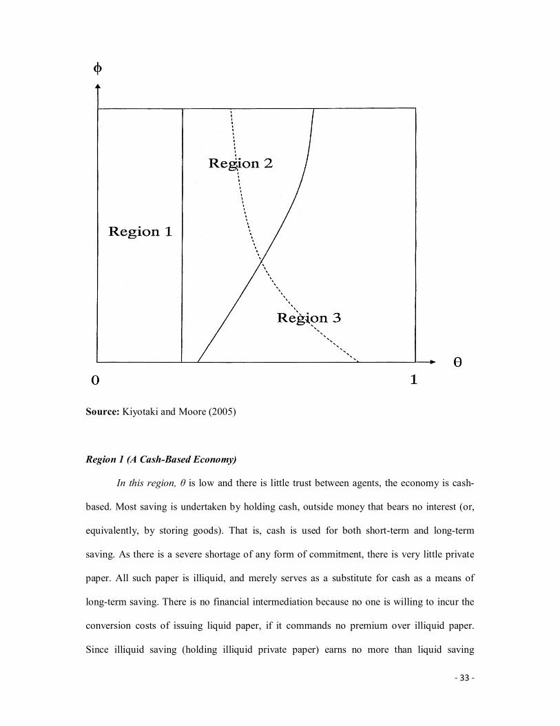
The “θ-φ model” predicts three stages of financial deepening, corresponding to three

different regions of the θ-φ parameter space, as shown in Fig 2.3

Fig 2.3 The three regions of financial deepening.

- 33 -

Source: Kiyotaki and Moore (2005)

Region 1 (A Cash-Based Economy)

In this region, θ is low and there is little trust between agents, the economy is cash-

based. Most saving is undertaken by holding cash, outside money that bears no interest (or,

equivalently, by storing goods). That is, cash is used for both short-term and long-term

saving. As there is a severe shortage of any form of commitment, there is very little private

paper. All such paper is illiquid, and merely serves as a substitute for cash as a means of

long-term saving. There is no financial intermediation because no one is willing to incur the

conversion costs of issuing liquid paper, if it commands no premium over illiquid paper.

Since illiquid saving (holding illiquid private paper) earns no more than liquid saving

- 34 -

(holding cash), agents are never “liquidity constrained”: they are never constrained by their

inability to resell private paper. However, agents with investment projects are “credit

constrained”: they would like to borrow more at the prevailing interest rate (zero), but are

constrained by the upper limit θ. Without adequate means of transferring resources from

savers to investors, the economy has too little investment. A rise in θ -financial deepening-

would boost investment and output. In the early Middle Ages prior to the development of

banking or negotiable financial instruments is a good example of this stage.

Region 2 (An Economy with Specialized Financial Markets)

In Region 2, where θ is higher and there is more trust, the economy enjoys specialized

financial markets, in the sense that liquid paper is used exclusively for short-term saving,

whereas illiquid paper is used for specific “point-to-point” long-term saving. Given its

versatility, liquid paper sells at a premium over illiquid paper -there is an interest rate

differential—and hence financial intermediation takes place: borrowers have an incentive to

incur the costs of converting some of their illiquid paper into liquid paper at the time of issue.

In saying that an economy has specialized financial markets, we mean the level of financial

intermediation is such that, in relative terms, the supplies of liquid and illiquid paper balance

the demands. The modern-day United State of America economy appears to be like this.

However, θ is still appreciably below unity- this implies that agents with investment projects

are still credit constrained. Given that too few resources are transferred from savers to

investors, further financial deepening, through a rise in θ or φ, would boost investment and

output in Region 2.

Region 3 (An Economy with Gross Financial Positions)

In an economy with a relatively high level of trust (θ high), if the costs of converting

to liquid paper are high (φ low), there can be an imbalance between the supplies of liquid and

illiquid paper. The markets are no longer specialized, in that savers resort to using

- 35 -

cumbersome long-term savings portfolios, holding different vintages of illiquid paper as a

surrogate for liquid saving. This is what distinguishes Region 3 from Region 2: without

adequate financial intermediation, agents hold gross financial positions, with illiquid paper

assets on both sides of their balance sheets. Arguably, the Japanese economy is currently in

Region 3, with large cross-holdings of trade credit (and equity), and too little netting out. In

financial terms, the economy is clogged up. Indeed, with enough trust (θ close to 1, the upper

part of Region 3), the economy can achieve first-best, despite the inconvenience of illiquid

paper. Here agents neither are credit constrained (interest rates match the return on

investment projects, and so the limit on borrowing, θ, is not binding), nor are liquidity

constrained.

Hervé Hannoun (2008) also identified four stages of financial deepening and its

sequencing over time:

The first stage of financial deepening is usually the emergence of banks. In an

economy where there is only very partial information about borrowers, banks are particularly

good at dealing with asymmetric information. Relationship lending allows banks to work

closely with borrowers to develop trust as well as to share information.

A second stage often involves the stock market. This usually comes later in the

financial system development process since it requires companies to publicly disclose

information about their business. But once this infrastructure is in place, the key advantage of

a well functioning stock market is that it provides something banks are not good at: a long-

term commitment of risk capital while still giving investors a liquid form of investment.

A third stage often emerges with the development of fixed income markets. These

markets, including both the bond markets and the money markets, are the markets of choice

for fundraising by governments, financial institutions and mature companies. The bond

markets provide good investment instruments for long-term investors such as pension funds

- 36 -

and insurance. The money markets are the place to manage short-term liquidity needs in large

quantities.

The final stage involves derivatives markets and securitization. Derivatives are

instruments for hedging risks. Securitization allows risks to be redistributed across investors

– a key step for the development of the so-called originate-to-distribute model of financing.

This final stage is what has given us the problems of the recent global turmoil.

2.5 IMPACT OF FINANCIAL DEEPENING ON ECONOMIC GROWTH

According to Dancheng (2008), financial deepening plays an important role in economic

growth and development:

i. Financial deepening can improve and enhance the allocation of resources. Finance has

the significant function of adjusting economic structure. First, it is to create favorable

conditions for readjustment of the industrial structure. In capital market, under the

premise of ownership, corporate assets can shift the enterprises resources from

industries or enterprises to the higher margin industries and the businesses through

securitization form, and change the resource allocation structure, which realize the

optimization and readjustment of the industrial structure. Secondly, it is to adjust the

industrial structure and expand sources of funds. Readjustment of the industrial

structure requires a large amount of incremental capital investment. Thirdly, it is to

widen the space of the industrial structure adjustment. Incremental investment is often

bounded by the sources of funds. Therefore, changes in the existing resources among

different industries and distribution can quickly realize the stock restructuring.

ii. Financial deepening can promote the capital formation. If a country has not sufficient

and sustained capital supply, it can not form a new economic growth point and

promote sustained and stable economic development. However, the capital formation

in a region is constrained by the level of savings in the region, but using the direct and

- 37 -

indirect means of financing, it can translate directly surplus funds of the inner region,

outside enterprises and residents into the investment capital by changing savings into

the investment indirectly or directly, this is the basic function of finance.

iii. Financial deepening can promote the reform of the corporate governance structure. A

country’s financial development, especially in the development of capital markets, not

only provides a convenient channel of financing for enterprises, and financing

mechanisms of capital markets can effectively promote the governance structure

change of the state-owned enterprises.

iv. Finance is the core of the modern economy, in the economic operation; it plays an

important role in guiding the flow of resources in the country and among countries

through special funds flow, which gets scarce resources in the region.

2.6 EMPIRICAL LITERATURE

The financial system serves as a catalyst to economic development through various

institutional structures. The system vigorously seek out and attract the reservoir of savings

and idle funds and allocate same to entrepreneurs, businesses, households and government for

investments projects and other purposes with a view of returns. This forms the basis for

economic development (Nzotta 2004:169).

Empirical evidence suggests that there are economies that have indeed benefited from

well-developed financial systems in the past. For some of the very successful emerging

market economies, finance appears to have been a crucial factor for economic success, e.g. in

Taiwan (Chang and Caudill, 2005). However, it is not always possible to identify such a

strong effect of finance on growth in mature OECD countries (Shan and Morris, 2002). For

developing economies, the results are similarly diverse. Some studies find a strong impact of

finance on growth (Tsionas, 2004), while others find the finance-growth relationship to be

more complex (Harb, 2005). The efficiency of financial markets in promoting financial

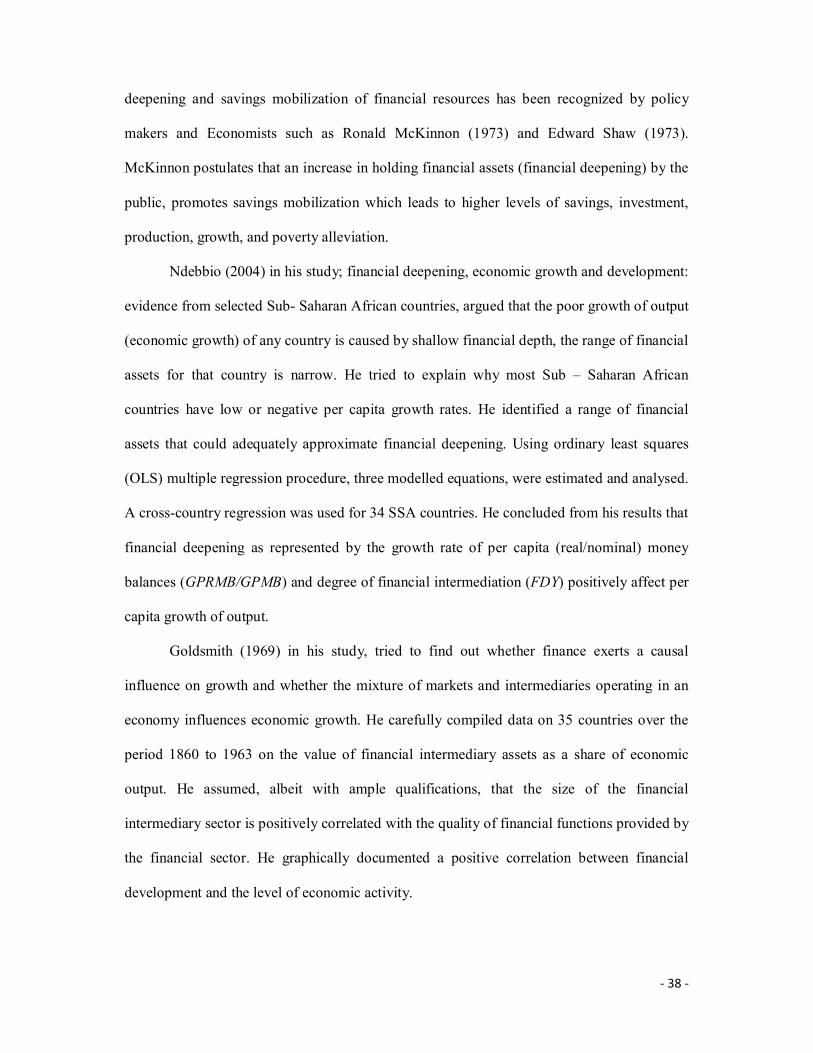
- 38 -

deepening and savings mobilization of financial resources has been recognized by policy

makers and Economists such as Ronald McKinnon (1973) and Edward Shaw (1973).

McKinnon postulates that an increase in holding financial assets (financial deepening) by the

public, promotes savings mobilization which leads to higher levels of savings, investment,

production, growth, and poverty alleviation.

Ndebbio (2004) in his study; financial deepening, economic growth and development:

evidence from selected Sub- Saharan African countries, argued that the poor growth of output

(economic growth) of any country is caused by shallow financial depth, the range of financial

assets for that country is narrow. He tried to explain why most Sub – Saharan African

countries have low or negative per capita growth rates. He identified a range of financial

assets that could adequately approximate financial deepening. Using ordinary least squares

(OLS) multiple regression procedure, three modelled equations, were estimated and analysed.

A cross-country regression was used for 34 SSA countries. He concluded from his results that

financial deepening as represented by the growth rate of per capita (real/nominal) money

balances (GPRMB/GPMB) and degree of financial intermediation (FDY) positively affect per

capita growth of output.

Goldsmith (1969) in his study, tried to find out whether finance exerts a causal

influence on growth and whether the mixture of markets and intermediaries operating in an

economy influences economic growth. He carefully compiled data on 35 countries over the

period 1860 to 1963 on the value of financial intermediary assets as a share of economic

output. He assumed, albeit with ample qualifications, that the size of the financial

intermediary sector is positively correlated with the quality of financial functions provided by

the financial sector. He graphically documented a positive correlation between financial

development and the level of economic activity.

- 39 -

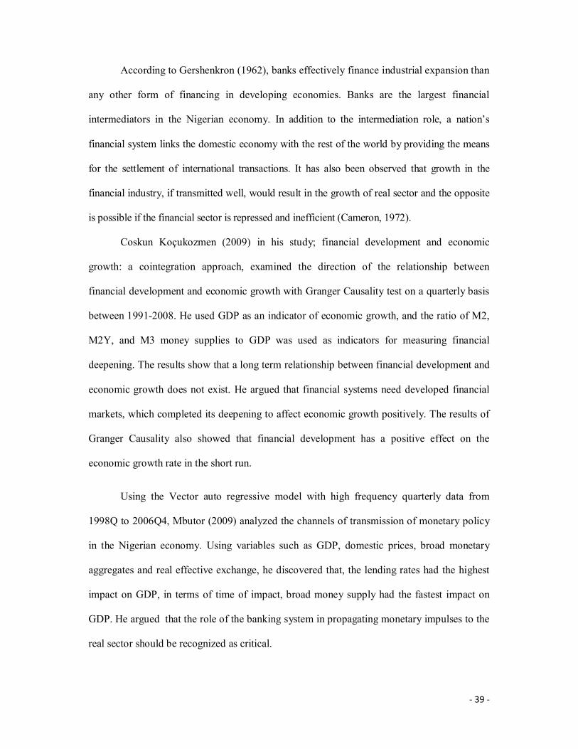
According to Gershenkron (1962), banks effectively finance industrial expansion than

any other form of financing in developing economies. Banks are the largest financial

intermediators in the Nigerian economy. In addition to the intermediation role, a nation’s

financial system links the domestic economy with the rest of the world by providing the means

for the settlement of international transactions. It has also been observed that growth in the

financial industry, if transmitted well, would result in the growth of real sector and the opposite

is possible if the financial sector is repressed and inefficient (Cameron, 1972).

Coskun Koçukozmen (2009) in his study; financial development and economic

growth: a cointegration approach, examined the direction of the relationship between

financial development and economic growth with Granger Causality test on a quarterly basis

between 1991-2008. He used GDP as an indicator of economic growth, and the ratio of M2,

M2Y, and M3 money supplies to GDP was used as indicators for measuring financial

deepening. The results show that a long term relationship between financial development and

economic growth does not exist. He argued that financial systems need developed financial

markets, which completed its deepening to affect economic growth positively. The results of

Granger Causality also showed that financial development has a positive effect on the

economic growth rate in the short run.

Using the Vector auto regressive model with high frequency quarterly data from

1998Q to 2006Q4, Mbutor (2009) analyzed the channels of transmission of monetary policy

in the Nigerian economy. Using variables such as GDP, domestic prices, broad monetary

aggregates and real effective exchange, he discovered that, the lending rates had the highest

impact on GDP, in terms of time of impact, broad money supply had the fastest impact on

GDP. He argued that the role of the banking system in propagating monetary impulses to the

real sector should be recognized as critical.

- 40 -

King and Levine (1993) conducted a study on seventy seven countries made up of

developed and developing economies used cross-country growth regression. The aim of

the research was to find out whether higher levels of financial development are

significantly and robustly correlated with faster current and future rates of economic growth,

physical capital accumulation and economic efficiency improvements. The result showed

that finance not only follows growth; finance seems important to lead economic growth.

Using panel integration and cointegration techniques for a dynamic heterogeneous

panel of 15 OECD and 50 non-OECD countries(65 countries in total) over the period 1975–

2000, Nicholas et’al(2006), examines whether a long-run relationship between financial

development and economic growth exists. In their study; Financial Deepening and Economic

Growth Linkages: A Panel Data Analysis, the specification used to test for cointegration and

causality between financial depth and growth was given as:

Yit = aoi + a1iFit + a2iXit + uit………………………… 1

Where: Yit is GDP per capita; Fit is a measure of financial development; Xit is a set of

control variables, and uit is the error term. Their results support a positive and statistically

significant equilibrium relation between financial development and economic growth for all

different financial indicators that was tested for and in all groups of countries.

Ayadi et’al, (2007) examine The Structural Adjustment, Financial Sector

Development and Economic Prosperity in Nigeria. They evaluated the structural adjustment

program in Nigeria, with a view to finding out if it resulted in an enhanced level of financial

development. Using the Spearman rank correlation, they examined the relationship between

financial development and economic growth during post-SAP period. They argued that the

extent of financial development depends on the volume of bank credit as well as the stock

market capitalization. They employed the use of some of the variables identified by Beck

et’al (2000) to test whether or not economic growth and financial development co-move since

- 41 -

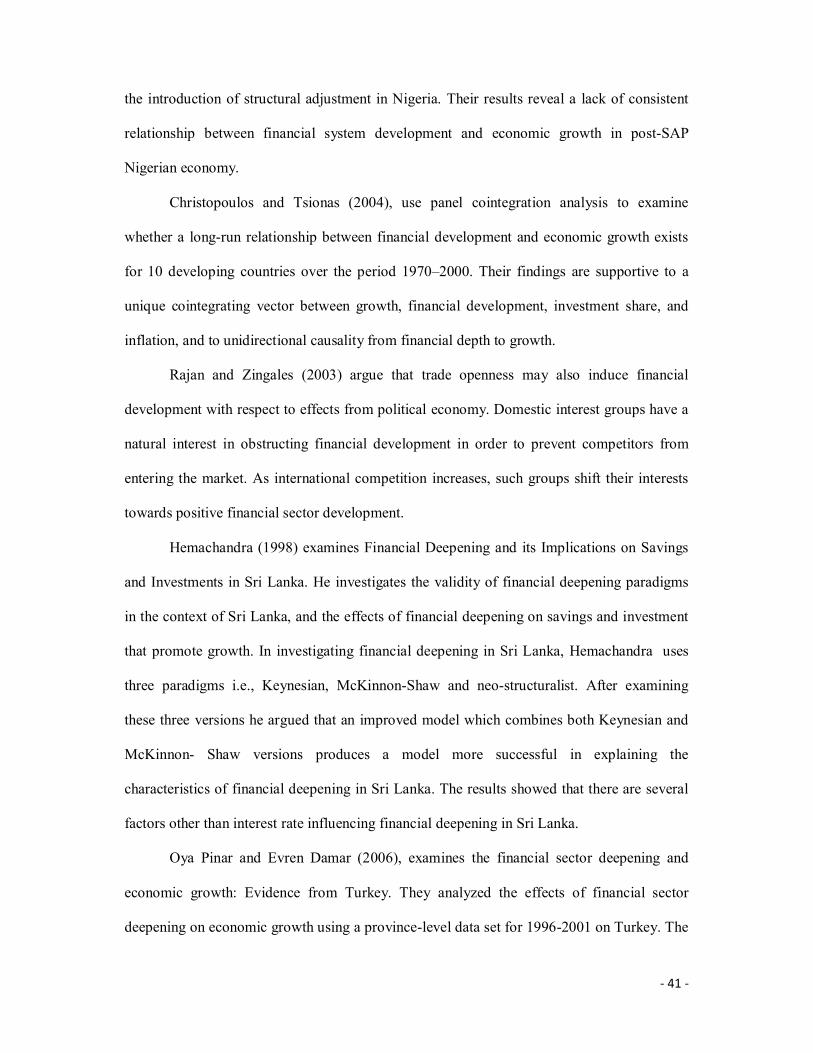
the introduction of structural adjustment in Nigeria. Their results reveal a lack of consistent

relationship between financial system development and economic growth in post-SAP

Nigerian economy.

Christopoulos and Tsionas (2004), use panel cointegration analysis to examine

whether a long-run relationship between financial development and economic growth exists

for 10 developing countries over the period 1970–2000. Their findings are supportive to a

unique cointegrating vector between growth, financial development, investment share, and

inflation, and to unidirectional causality from financial depth to growth.

Rajan and Zingales (2003) argue that trade openness may also induce financial

development with respect to effects from political economy. Domestic interest groups have a

natural interest in obstructing financial development in order to prevent competitors from

entering the market. As international competition increases, such groups shift their interests

towards positive financial sector development.

Hemachandra (1998) examines Financial Deepening and its Implications on Savings

and Investments in Sri Lanka. He investigates the validity of financial deepening paradigms

in the context of Sri Lanka, and the effects of financial deepening on savings and investment

that promote growth. In investigating financial deepening in Sri Lanka, Hemachandra uses

three paradigms i.e., Keynesian, McKinnon-Shaw and neo-structuralist. After examining

these three versions he argued that an improved model which combines both Keynesian and

McKinnon- Shaw versions produces a model more successful in explaining the

characteristics of financial deepening in Sri Lanka. The results showed that there are several

factors other than interest rate influencing financial deepening in Sri Lanka.

Oya Pinar and Evren Damar (2006), examines the financial sector deepening and

economic growth: Evidence from Turkey. They analyzed the effects of financial sector

deepening on economic growth using a province-level data set for 1996-2001 on Turkey. The

- 42 -

analysis was carried out using two different methods: cross-section analysis and dynamic

panel data analysis. Using both traditional OLS and dynamic panel GMM techniques, the

results showed that financial deepening (i.e. an increase in the total deposits to GDP ratio)

has a direct and robust impact on the growth rate of real GDP per capita. However, unlike

most of the cross-country studies in this literature, the findings suggest that financial

development has a negative relationship to economic growth.

Gries et’al (2009) investigates the direct and indirect causal interactions between

financial deepening, trade openness and economic growth for 13 Latin American and

Caribbean countries. They employed unit root and cointegration tests to identify the

stationary properties and possible cointegration relationships of the investigated time series,

employing Hsiao's version of Granger causality within a autoregressive (VAR) or vector error

correction models (VECM) framework. Findings from the result showed that for Latin

America and the Caribbean, they detected almost no evidence of finance led growth, most

results pointed at a demand-following or insignificant causal interaction between finance and

growth in the Latin American region.

- 43 -

CHAPTER THREE

METHODOLOGY

3.1 INTRODUCTION

In this part of the study, the relationship between financial deepening and economic

growth in Nigeria was examined. To serve our purpose, appropriate variables will be

established and the causal relationships between these variables determined by using

econometric estimation methods.

3.2 SOURCE OF DATA

The data employed in this research work are annual time series data of relevant

variables and the data are mainly secondary. The data were collected from publications of the

Central Bank of Nigeria (CBN), Federal Office of Statistics (FOS) and World Bank

publications. Financial deepening was defined as the ratio of money supply to GDP, and it is

a function of money supply to GDP, value of cheques to money supply, ratio of private sector

credit to GDP, financial savings to GDP, rate of inflation, real lending rates, deposit money

bank assets to GDP, and Currency outside Banks to money supply. The prime lending rates

of the banks shall be used to stand for interest rate (the long term interest).

3.3 ANALYTICAL TECHNIQUE

If the series variables for this study are stationary and no causality exists, the

Autoregressive Distributed Lag model (ADL) will be used in estimating the parameters of the

model. However, if the variables are not stationary and there exist no causality, Error

Correction Model (ECM) will be applied. But if there is causality and the variables are still

not stationary (they cointegrate), Vector Error Correction (VEC) model will be applied.

Furthermore, if the variables are stationary and there is causality and they do not cointegrate,

the Vector Autoregressive (VAR) model will be used to estimate the parameters of the

model.

- 44 -

From our literature, we adopted and specified the VAR model used by Coskun

(2009). The VAR model has proven to be especially useful for describing the dynamic

behavior of economic and financial time series and for forecasting (Sims, 1980). Forecasts

from VAR models are quite flexible because they can be made conditional on the potential

future paths of specified variables in the model. These impacts are usually summarized with

impulse response functions and forecast error variance decompositions. The vector

autoregression (VAR) method, being a data-induced technique places a minimal theoretical

emphasis on the structural relationship, but simply involves the specification of the set of

endogenous variables that are believed to have logical relationship and qualify for inclusion

as part of the economic system. The Vector autoregressive (VAR) is used for estimating

systems of interrelated time series and for analyzing the dynamic impact of random

disturbances on the system of variables.

3.4 MODEL SPECIFICATION

The bench mark for the above model can be specified as:

GDPt = f (FDt) ………………………………………………….1

FDt = (MSGt, PLRt, FSGt, CHMt INFt, PCGt, DBGt, COBMt) ………….2

Where:

GDPt = Gross Domestic Product

FDt = Financial Deepening

MSGt = Money supply/GDP ratio (M2/GDP)

FSGt = Financial Savings/GDP ratio (FS/DGP)

CHMt = Value of Cheques Cleared to Money Supply (CHQ/MS2)

PCGt = Ratio of Private Sector Credit to GDP (PSC/GDP

- 45 -

DBGt = Ratio of Deposit Money Bank Asset to GDP (DBMA/GDP)

INFt = Rate of Inflation

PLRt = Prime lending rates

COBMt = Currency outside Banks to Money Supply (COB/MS2)

The above variables were logged to take care of non-linear phenomena. Thus, we

consider a restricted standard form of our VAR model with lag order k, as:

Yt = µ + ∑ 퐴iYt-1 + εt . . .. . . ………………….. 2

Where Yt is an (n x 1) vector of endogenous variables, µ is a vector of constants, while Y

is the corresponding lag term for each of the variables. A is an (nxn) matrix of

autoregressive coefficient vector ofY , εt is a vector of white noise processes.

THE MODEL

9t

8t

7t

6t

5t

4t

3t

2t

1t

1

1

1

1

1

1

1

1

1-

9i9i9i9i9i9i9i9i9i

8i8i8i8i8i8i8i8i8i

7i7i7i7i7i7i7i7i7i

6i6i6i6i6i6i6i6i6i

5i5i5i5i5i5i5i5i5i

4i4i4i4i4i4i4i4i4i

3i3i3i3i3i3i3i3i3i

2i2i2i2i2i2i2i2i2i

1i1i 1i1i1i1i1i1i1i

k1i

i h g f e d c b ai h g f e d c b ai h g f e d c b ai h g f e d c b ai h g f e d c b ai h g f e d c b ai h g f e d c b ai h g f e d c b a

i h g f e d c b a

t

t

t

t

t

t

t

t

t

t

t

t

t

t

t

t

t

t

COBMPLRINFDBGPCGCHMMSGFSG

PG

COBMPLRINFDBGPCGCHMMSGFSG

PG DD

………….. 3

Where aij, bij, cij, dij, eij,fij,gij,hij, and iij are coefficients of GDPt, FSGt, MSGt, CHMt, PCGt,

DBGt, INFt, PLRt and COBMt respectively t are error terms assumed to be a white noise

process and t-i are the lagged values of each series up to the p-lag.

- 46 -

3.5 ESTIMATION TECHNIQUE

3.5.1 UNIT ROOT TEST

There are several reasons why the concept of non-stationarity is important. A stationary series

have a zero mean and constant variance. One of the methods to test whether series is

stationary or not is Dickey-Fuller (DF) (1979), DF test is very important in terms of

measuring which degree stationary series have, but it does not consider an autocorrelation in

disturbance term. If disturbance term contains autocorrelation, DF test is invalid. In this

situation, by adding lagged terms of dependent variable to explanatory variable, generalized

Dickey Fuller (Augmented Dickey-Fuller) is used ( Brooks, 2002).

The ADF test, can be defined as follows

∆Yt = Y0 + αt + Φ Yt-1 + ∑ Φ iYt-1 +µt …………………………………4

∆Yt = Yt - Yt-1 ……………………………………………………… 5

Where:

Yt = dependent variable

Y0 = constant term

T = trend variable

Ut = stochastic disturbance term

There are hypotheses to test series

H0 : Φ = 0 (Yt is non-stationary)

H1 : Φ ≠ 0 (Yt is not non-stationary)

ADF is a regress test using each series own lagged terms with big differences. Many

econometric programs satisfy ADF test statistics. If calculated t-value of variable is greater

than ADF critical t-value, then H0 is rejected and thus the data is stationary. It will be

- 47 -

compared with the Mckinnon critical values, if ADF test statistic is greater than McKinnon

critical values absolutely, the series are stationary at that level.

3.5.2 GRANGER CAUSALITY TEST

If there is a lagged relationship between two variables, one of the test, which is applied to

determine the direction of relation in terms of statistics, is Granger Causality test. Granger

Causality test also gives information about the short-term relationship between the variables

(Granger and Engle, 1987).

Even there are different ideas about causality in terms of conceptional definition, this concept

makes a relation between causes and results. Conceptional definition of causality depends on

Aristo’s assumption. According to Aristo, there is a relationship between causes and results

and these results cannot occur without causes. This relationship is a strong relationship.

Granger’s operational causality definition depends on the hypotheses below:

i. Certain causality is possible only with past causes present time or future time. Cause is

always to be come true before the result. In addition, this makes time lagged between causes

and results.

ii. Causality can be determined only stochastic process. It is not possible to determine the

causality between two deterministic processes.

Yt = α + ∑βjXt-j + ∑ ΦiYt-I + Ut ………………………………….6

Xt = α + ∑βjYt-j + ∑ ΦiXt-j + Ut …………………………………7

In Granger Causality test, there are three possible situations that one directional causality

from x to y or y to x, opposite direction between x and y or one affect the other and

independency of x and y each other. This situation changes according to the null hypothesis

and lagged values randomly in equations above whose parameters are whether equal to zero

or not. According to researches, randomly choice makes causality incline to deviations

importantly. Indicators of the economic growth and the financial deepening are variables,

- 48 -

which are used for Granger Causality test. Moreover, this test can determine the effects of

one variable on the other.

3.5.3 IMPULSE RESPONSE FUNCTIONS

An impulse-response function traces the effect of a one-time shock to one of the

innovations on the current and future values of the endogenous variables. The impulse

response functions can be used to produce the time path of the dependent variables in the

VAR, to shocks from all the explanatory variables. If the system of equations is stable any

shock should decline to zero, an unstable system would produce an explosive time path. It

simply refers to the reaction of any dynamic system in response to some external change. In

both cases, the impulse response describes the reaction of the system as a function of time (or

possibly as a function of some other independent variable that parameterizes the dynamic

behavior of the system).

Innovations in financial deepening will certainly affect economic growth either

positively or negatively. We shall therefore use the impulse-response function to trace the

effect of innovations in financial deepening on economic growth.

3.5.4 VARIANCE DECOMPOSITION ANALYSIS (VDA)

The Variance Decomposition is an alternative method to the impulse response functions

for examining the effects of shocks to the dependent variables. This technique determines

how much of the forecast error variance for any variable in a system, is explained by

innovations to each explanatory variable, over a series of time horizons.

The Variance Decomposition provides information about the relative importance of each

random innovation in affecting the random variables in the VAR (Hamilton, 1994).

Therefore, Variance Decompositions show the proportion of forecast error variance that is

- 49 -

attributable to its own innovation and to innovations from other endogenous variables in the

model.

3.6 A PRIORI EXPECTATIONS

It is expected that at the end of this study to either see that financial deepening influences

economic growth, with MSG, PCG, VCM, FSG and DBM having a positive relationship with

GDP, supporting the supplying leading hypothesis, or see that it is economic growth that

exerts influence on the financial system supporting the demand following hypothesis.

- 50 -

CHAPTER FOUR

DATA ANALYSIS AND PRESENTAION OF RESULTS

4.1 INTRODUCTION

This chapter is basically divided into two. Section 4.2 presents the trend, structure and

growth of financial deepening in Nigeria, while section 4.3 presents empirical analysis.

4.2 TREND, STRUCTURE AND GROWTH OF FINANCIAL DEEPENING NIGERIA

Until recently, with the recapitalization in the banking sector which resulted in

mergers and acquisitions, increased bank branches and innovations of new products and

technology coupled with growth in the capital markets, the Nigerian financial system

remained by and large relatively underdeveloped because of lack of financial intermediation

and financial deepening which the economy requires for sustained growth. In Nigeria

however, the influence of money supply on economic growth can only be taken with mixed

reactions. Between 1971 and 1975, the growth rate of the economy measured by the real

GDP ranged from 21.3% in 1971 to 3.0% in 1975.

By 1981, the real GDP grew by 26.8% and remained negative till 1984. A simple

variance analysis shows that between 1971 and 1986, the mean spread of the GDP was 108.7.

However, between 1986 and 1994, the real GDP had a variance of 9.1. The variability of the

GDP was much higher before deregulation, while it becomes lower during and after the

deregulation of the economy. Both M1 and M2 had little correlation with growth of real GDP

before deregulation in 1986. M2 was observed to have a variance of 362.6 and a correlation

coefficient of 0.21.

The period 1986-1994 had a lower correlation of 0.16 between broadmoney (M2) and

growth of real GDP. The mean spread of M2 was 289.2 as against 108.7 for the real GDP.

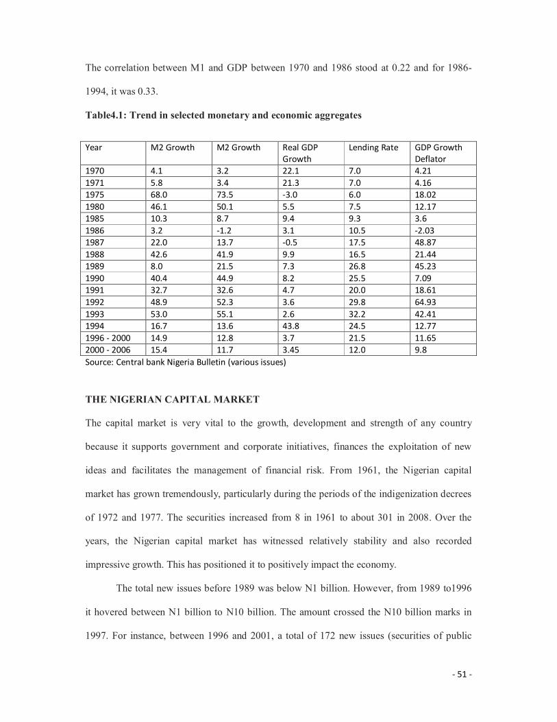
- 51 -

The correlation between M1 and GDP between 1970 and 1986 stood at 0.22 and for 1986-

1994, it was 0.33.

Table4.1: Trend in selected monetary and economic aggregates

Year M2 Growth M2 Growth Real GDP Growth

Lending Rate GDP Growth Deflator

1970 4.1 3.2 22.1 7.0 4.21 1971 5.8 3.4 21.3 7.0 4.16 1975 68.0 73.5 -3.0 6.0 18.02 1980 46.1 50.1 5.5 7.5 12.17 1985 10.3 8.7 9.4 9.3 3.6 1986 3.2 -1.2 3.1 10.5 -2.03 1987 22.0 13.7 -0.5 17.5 48.87 1988 42.6 41.9 9.9 16.5 21.44 1989 8.0 21.5 7.3 26.8 45.23 1990 40.4 44.9 8.2 25.5 7.09 1991 32.7 32.6 4.7 20.0 18.61 1992 48.9 52.3 3.6 29.8 64.93 1993 53.0 55.1 2.6 32.2 42.41 1994 16.7 13.6 43.8 24.5 12.77 1996 - 2000 14.9 12.8 3.7 21.5 11.65 2000 - 2006 15.4 11.7 3.45 12.0 9.8 Source: Central bank Nigeria Bulletin (various issues)

THE NIGERIAN CAPITAL MARKET

The capital market is very vital to the growth, development and strength of any country

because it supports government and corporate initiatives, finances the exploitation of new

ideas and facilitates the management of financial risk. From 1961, the Nigerian capital

market has grown tremendously, particularly during the periods of the indigenization decrees

of 1972 and 1977. The securities increased from 8 in 1961 to about 301 in 2008. Over the

years, the Nigerian capital market has witnessed relatively stability and also recorded

impressive growth. This has positioned it to positively impact the economy.

The total new issues before 1989 was below N1 billion. However, from 1989 to1996

it hovered between N1 billion to N10 billion. The amount crossed the N10 billion marks in

1997. For instance, between 1996 and 2001, a total of 172 new issues (securities of public

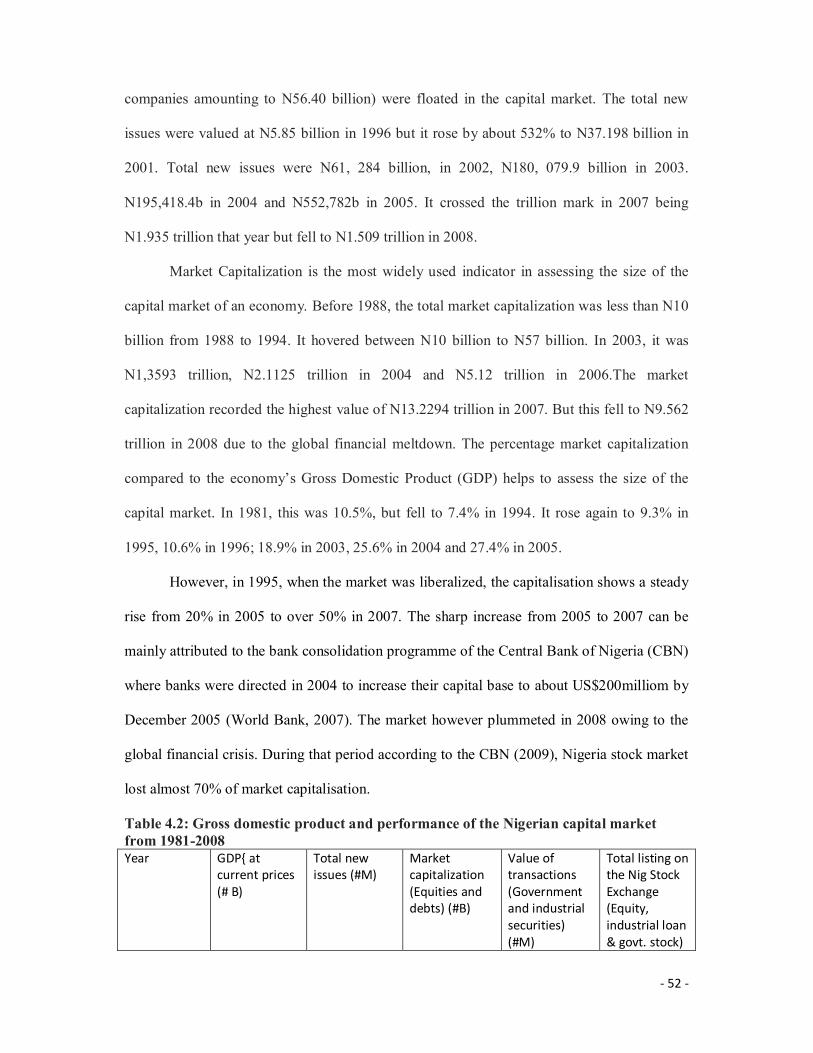
- 52 -

companies amounting to N56.40 billion) were floated in the capital market. The total new

issues were valued at N5.85 billion in 1996 but it rose by about 532% to N37.198 billion in

2001. Total new issues were N61, 284 billion, in 2002, N180, 079.9 billion in 2003.

N195,418.4b in 2004 and N552,782b in 2005. It crossed the trillion mark in 2007 being

N1.935 trillion that year but fell to N1.509 trillion in 2008.

Market Capitalization is the most widely used indicator in assessing the size of the

capital market of an economy. Before 1988, the total market capitalization was less than N10

billion from 1988 to 1994. It hovered between N10 billion to N57 billion. In 2003, it was

N1,3593 trillion, N2.1125 trillion in 2004 and N5.12 trillion in 2006.The market

capitalization recorded the highest value of N13.2294 trillion in 2007. But this fell to N9.562

trillion in 2008 due to the global financial meltdown. The percentage market capitalization

compared to the economy’s Gross Domestic Product (GDP) helps to assess the size of the

capital market. In 1981, this was 10.5%, but fell to 7.4% in 1994. It rose again to 9.3% in

1995, 10.6% in 1996; 18.9% in 2003, 25.6% in 2004 and 27.4% in 2005.

However, in 1995, when the market was liberalized, the capitalisation shows a steady

rise from 20% in 2005 to over 50% in 2007. The sharp increase from 2005 to 2007 can be

mainly attributed to the bank consolidation programme of the Central Bank of Nigeria (CBN)

where banks were directed in 2004 to increase their capital base to about US$200milliom by

December 2005 (World Bank, 2007). The market however plummeted in 2008 owing to the

global financial crisis. During that period according to the CBN (2009), Nigeria stock market

lost almost 70% of market capitalisation.

Table 4.2: Gross domestic product and performance of the Nigerian capital market from 1981-2008 Year GDP{ at

current prices (# B)

Total new issues (#M)

Market capitalization (Equities and debts) (#B)

Value of transactions (Government and industrial securities) (#M)

Total listing on the Nig Stock Exchange (Equity, industrial loan & govt. stock)

- 53 -

1986 205,971.4 833.0 6,794.8 494.4 240 1987 204,806.5 450.7 8,297.6 348.0 244 1988 219,876.8 400.0 10,020.8 137.6 253 1989 263,729.6 1,629.9 12,848.6 521.6 267 1990 267,660 9,964.5 16,358.4 265.5 295 1991 265,379.1 1,870.0 23,125.0 136.0 239 1992 271,365.5 3,306.3 31,272.6 313.5 251 1993 274,833.3 2,636.9 47,436.1 402.3 272 1994 275,450.6 2,161.7 66,3680 569.7 276 1995 281,407.4 4,425.6 180,305.1 1,838.8 276 1996 293,745.4 5858.2 281,815.8 7,062.7 276 1997 302,022.5 10,875.7 281,887.2 11,072.7 264 1998 310,890.1 15,018.1 262,517.3 13,572.3 264 1999 312,183.5 12,038.5 300.041.1 14,027.4 268 2000 329,978.7 17,207.8 472.290.0 28,154.6 260 2001 356,994.3 37,198.8 662,561.3 57,6372 261 2002 433,203.5 61,284.0 764,975.8 60,088.6 258 2003 477,833 180,079.9 1,359,274.2 120,703.0 265 2004 527,576 195,418.4 2,112,549.6 225,820.6 277 2005 561.931.4 552,782 2,900,062.1 262,929.6 288 2006 595,821.6 707,400 5,120,000 470,253.0 294 2007 634,251 1,935,080 13,294,059 2,100,000 310 2008 674,889 1,509,230 9,562,970 4,400,000 301 Source: SEC, NSE, CBN (Various issues)

Some selected indicators of financial deepening are highlighted below. From the table

4.3, we can see the trend of money supply (M2), credit o the private sector and Gross

domestic product. Also, included are the ratios of M2 to GDP and credit to the private sector

and GDP. In 1986, M2/GDP ratio was 34.43%, it fell to 14% in 1995, it started rising, and by

2001 it was 26%, by 2010, it had risen to 37%. However, we could see a level of

inconsistencies and fluctuations over the years.

Table 4.3: Selected Financial Deepening Indicators

Year

Money Supply2

(M2) (N' Million)

Credit to Private Sector2

(N' Million)

GDP at Current Basic Prices (N' Million)

Financial Deepening

(M2/GDP) (%)

(CPS/GDP) (%)

1986 23,806.40 15,247.45 69,146.99 34.43 22.05 1987 27,573.58 21,082.99 105,222.84 26.20 20.04 1988 38,356.80 27,326.42 139,085.30 27.58 19.65 1989 45,902.88 30,403.22 216,797.54 21.17 14.02 1990 52,857.03 33,547.70 267,549.99 19.76 12.54 1991 75,401.18 41,352.46 312,139.74 24.16 13.25 1992 111,112.31 58,122.95 532,613.83 20.86 10.91

- 54 -

1993 165,338.75 127,117.71 683,869.79 24.18 18.59 1994 230,292.60 143,424.21 899,863.22 25.59 15.94 1995 289,091.07 180,004.76 1,933,211.55 14.95 9.31 1996 345,853.96 238,596.56 2,702,719.13 12.80 8.83 1997 413,280.13 316,207.08 2,801,972.58 14.75 11.29 1998 488,145.79 351,956.19 2,708,430.86 18.02 12.99 1999 628,952.16 431,168.36 3,194,014.97 19.69 13.50 2000 878,457.27 530,373.30 4,582,127.29 19.17 11.57 2001 1,269,321.61 764,961.52 4,725,086.00 26.86 16.19 2002 1,508,172.91 930,493.93 6,912,381.25 21.82 13.46 2003 1,952,922.28 1,096,535.57 8,487,031.57 23.01 12.92 2004 2,131,820.08 1,421,664.03 11,411,066.91 18.68 12.46 2005 2,637,913.73 1,838,389.93 14,572,239.12 18.10 12.62 2006 3,799,538.05 2,290,617.76 18,564,594.73 20.47 12.34

2007 1 5,138,700.94 3,680,090.19 20,657,317.66 24.88 17.81 2008 1 8,029,088.61 6,941,383.41 24,296,329.29 33.05 28.57 2009 1 9,456,480.31 9,147,417.17 24,794,238.66 38.14 36.89 2010 11,034,940.93 10,157,021.18 29,205,782.96 37.78 34.78

Sources: Central Bank of Nigeria and National Bureau of Statistics (2011)

4.3.1 UNIT ROOT TEST

This research work began with the investigation of the time series properties of each

variable employed in the study by using both the Augmented Dickey Fuller (ADF) and

Phillip Peron (PP) tests to determine the order of integration of the series. Table 4.4 shows

that the two tests are consistent, suggesting that GDP, INF, PLR, FSG, PSG, and DMBA are

all stationary at first difference which implies that, they all integrated of order one, while

MSG, VCM and COBM are stationary at second difference, meaning they are integrated of

order two. Since the series are not integrated of the same order, it therefore excludes the

possibility of a long run relationship among the variables, which implies the cointegration test

is not necessary. Therefore the analysis of this study proceeded with the Vector

Autoregressive approach.

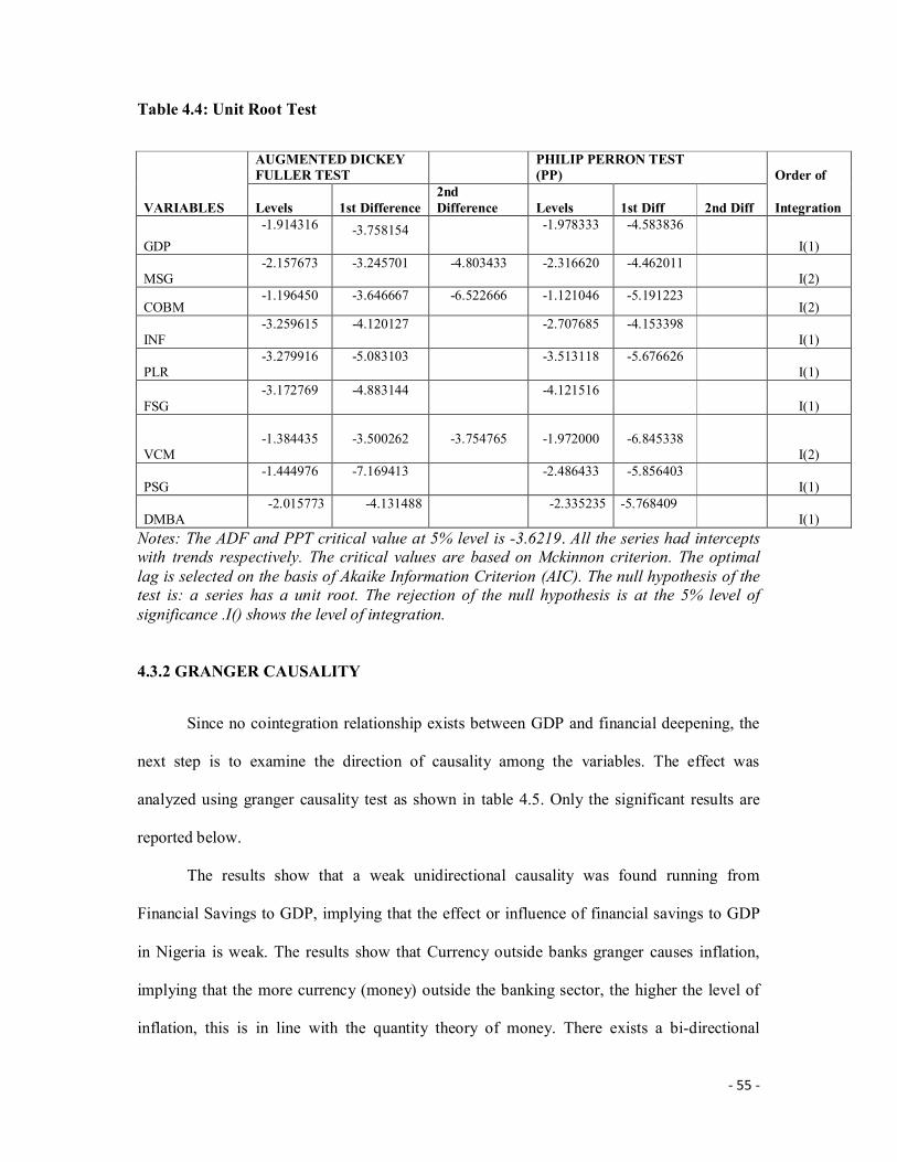
- 55 -

Table 4.4: Unit Root Test

VARIABLES

AUGMENTED DICKEY FULLER TEST

PHILIP PERRON TEST (PP) Order of

Levels 1st Difference 2nd Difference Levels 1st Diff 2nd Diff Integration

GDP -1.914316 -3.758154

-1.978333 -4.583836

I(1)

MSG -2.157673 -3.245701 -4.803433

-2.316620

-4.462011

I(2)

COBM -1.196450 -3.646667 -6.522666 -1.121046 -5.191223

I(2)

INF -3.259615 -4.120127

-2.707685

-4.153398

I(1)

PLR -3.279916

-5.083103

-3.513118

-5.676626

I(1)

FSG -3.172769

-4.883144

-4.121516

I(1)

VCM -1.384435

-3.500262

-3.754765

-1.972000

-6.845338

I(2)

PSG -1.444976

-7.169413

-2.486433

-5.856403

I(1)

DMBA -2.015773

-4.131488

-2.335235

-5.768409 I(1)

Notes: The ADF and PPT critical value at 5% level is -3.6219. All the series had intercepts with trends respectively. The critical values are based on Mckinnon criterion. The optimal lag is selected on the basis of Akaike Information Criterion (AIC). The null hypothesis of the test is: a series has a unit root. The rejection of the null hypothesis is at the 5% level of significance .I() shows the level of integration.

4.3.2 GRANGER CAUSALITY

Since no cointegration relationship exists between GDP and financial deepening, the

next step is to examine the direction of causality among the variables. The effect was

analyzed using granger causality test as shown in table 4.5. Only the significant results are

reported below.

The results show that a weak unidirectional causality was found running from

Financial Savings to GDP, implying that the effect or influence of financial savings to GDP

in Nigeria is weak. The results show that Currency outside banks granger causes inflation,

implying that the more currency (money) outside the banking sector, the higher the level of

inflation, this is in line with the quantity theory of money. There exists a bi-directional

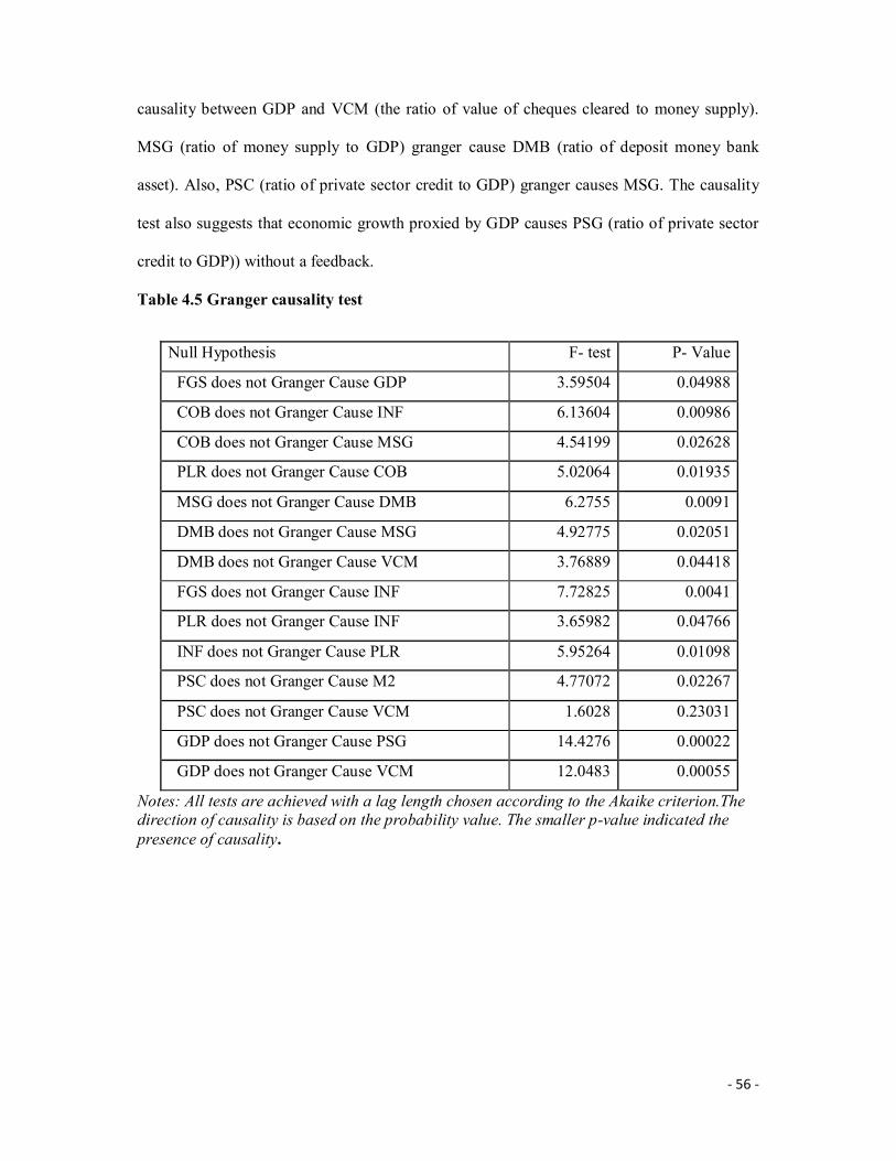
- 56 -

causality between GDP and VCM (the ratio of value of cheques cleared to money supply).

MSG (ratio of money supply to GDP) granger cause DMB (ratio of deposit money bank

asset). Also, PSC (ratio of private sector credit to GDP) granger causes MSG. The causality

test also suggests that economic growth proxied by GDP causes PSG (ratio of private sector

credit to GDP)) without a feedback.

Table 4.5 Granger causality test

Null Hypothesis F- test P- Value

FGS does not Granger Cause GDP 3.59504 0.04988

COB does not Granger Cause INF 6.13604 0.00986

COB does not Granger Cause MSG 4.54199 0.02628

PLR does not Granger Cause COB 5.02064 0.01935

MSG does not Granger Cause DMB 6.2755 0.0091

DMB does not Granger Cause MSG 4.92775 0.02051

DMB does not Granger Cause VCM 3.76889 0.04418

FGS does not Granger Cause INF 7.72825 0.0041

PLR does not Granger Cause INF 3.65982 0.04766

INF does not Granger Cause PLR 5.95264 0.01098

PSC does not Granger Cause M2 4.77072 0.02267

PSC does not Granger Cause VCM 1.6028 0.23031

GDP does not Granger Cause PSG 14.4276 0.00022

GDP does not Granger Cause VCM 12.0483 0.00055

Notes: All tests are achieved with a lag length chosen according to the Akaike criterion.The direction of causality is based on the probability value. The smaller p-value indicated the presence of causality.

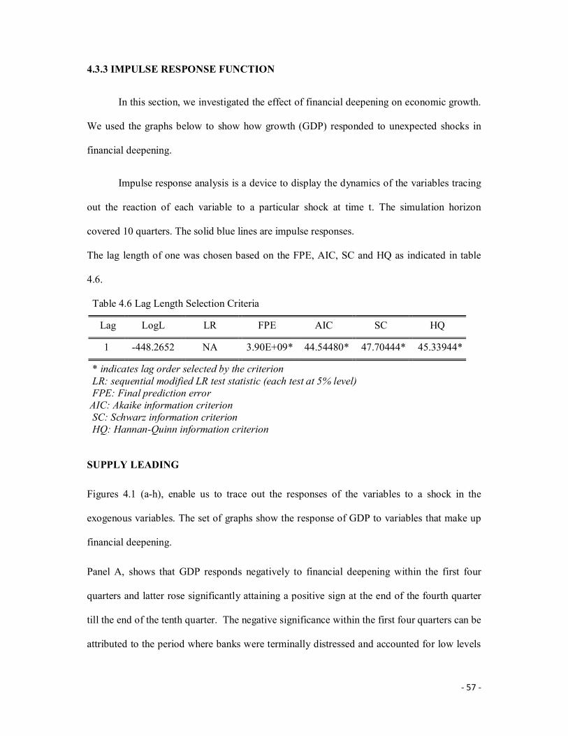
- 57 -

4.3.3 IMPULSE RESPONSE FUNCTION

In this section, we investigated the effect of financial deepening on economic growth.

We used the graphs below to show how growth (GDP) responded to unexpected shocks in

financial deepening.

Impulse response analysis is a device to display the dynamics of the variables tracing

out the reaction of each variable to a particular shock at time t. The simulation horizon

covered 10 quarters. The solid blue lines are impulse responses.

The lag length of one was chosen based on the FPE, AIC, SC and HQ as indicated in table

4.6.

Table 4.6 Lag Length Selection Criteria

Lag LogL LR FPE AIC SC HQ

1 -448.2652 NA 3.90E+09* 44.54480* 47.70444* 45.33944*

* indicates lag order selected by the criterion LR: sequential modified LR test statistic (each test at 5% level) FPE: Final prediction error AIC: Akaike information criterion SC: Schwarz information criterion HQ: Hannan-Quinn information criterion

SUPPLY LEADING

Figures 4.1 (a-h), enable us to trace out the responses of the variables to a shock in the

exogenous variables. The set of graphs show the response of GDP to variables that make up

financial deepening.

Panel A, shows that GDP responds negatively to financial deepening within the first four

quarters and latter rose significantly attaining a positive sign at the end of the fourth quarter

till the end of the tenth quarter. The negative significance within the first four quarters can be

attributed to the period where banks were terminally distressed and accounted for low levels

- 58 -

of financial deepening. The fact that GDP rises thereafter from a negative to attain a positive

sign suggest that deepening of the financial markets can lead to a significant growth in the

long run. This lends credence to the supply leading hypothesis that financial deepening

causes economic growth.

Panel B indicates that private sector credit (PSC) impacts positively on economic growth

(GDP). That is GDP responds positively to an unexpected shock in PSC within the first four

quarters, and further increases significantly till the end of the tenth quarter. The implication

of this finding is that, sustaining desired levels of new investments through private sector

credit will facilitate growth in the economy. Although the level of interest rates have

remained very high, the level of private sector credits have not sustained the desired levels of

new investments through private sector credit to facilitate growth in the economy.

Panel C, shows an unexpected shock in inflation leads to a constant rise in GDP. This result

is in line with our a priori expectations. A mild level of inflation stimulates investment and

consequently growth.

We observed from panel D that, GDP increased from negative to positive within the first two

quarters when financial savings increase by one standard deviation and there after declines

persistently till the end of the last quarter. This result suggests that economic growth cannot

be sustained by banks’ savings.

In panel E below, we observed that GDP responds negatively to checks outside banks. The

implication is that if more checks are issued into the economy, this will slow down economic

activities.

Panel F shows the response of real GDP to an expansionary shock in the prime lending rate

(PLR). Within the first two years, GDP is stable with changes in PLR. At the end of the

second quarter, GDP rises quickly and significantly and further increases up to the fourth

- 59 -

quarter. And almost stabilizes till the end of the last quarter. This suggests that financial

deepening with respect to the prime lending rates would lead to a high and sustainable

economic growth in Nigeria.

In Panel G, we observe that a positive innovation in deposit money outside bank (DMB) has

a positive effect on GDP in the first three quarters and then it fizzles out in the fourth quarter.

At the end of the fourth quarter till the last quarter, GDP responds negatively to unexpected

shocks in DMB. This suggests that if more deposits are held by non-financial banks

(institutions), GDP will drop significantly.

In Panel H below, a one standard deviation increase in currency outside bank, leads to

significant rise in GDP reaching its maximum in the third quarter and thereafter declines

gradually till the end of the last quarter maintaining its positive sign. This suggests that more

currency outside bank will leave more cash balances with individuals in the economy thus

increasing the level of demand for goods and services which in turn increases the level of

investment thus increasing the level of GDP.

FIGURE 4.1(a-h): IMPULSE RESPONSE FUNCTIONS OF GDP TO A SHOCK IN

THE EXPLANATORY VARIABLES

Panel a Panel b

-.15

-.10

-.05

.00

.05

.10

.15

1 2 3 4 5 6 7 8 9 10

Response of GDP1 to CholeskyOne S.D. M2 Innovation

-.10

-.05

.00

.05

.10

.15

.20

1 2 3 4 5 6 7 8 9 10

Response of GDP1 to CholeskyOne S.D. PSC Innovation

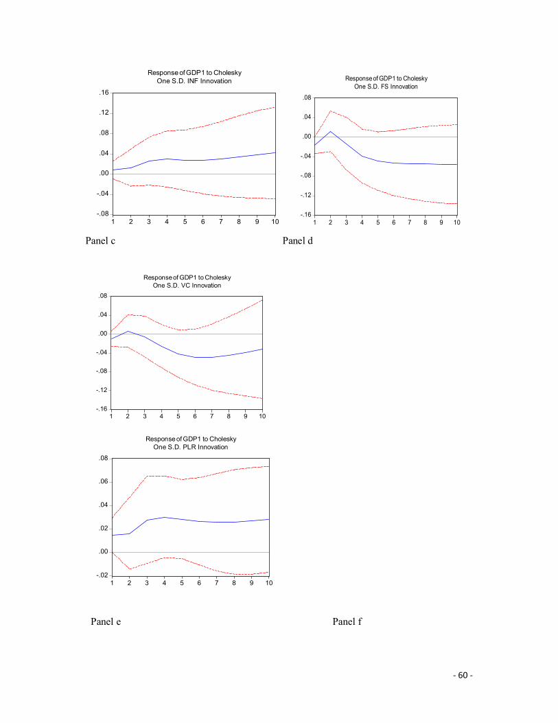
- 60 -

Panel c Panel d

Panel e Panel f

-.08

-.04

.00

.04

.08

.12

.16

1 2 3 4 5 6 7 8 9 10

Response of GDP1 to CholeskyOne S.D. INF Innovation

-.16

-.12

-.08

-.04

.00

.04

.08

1 2 3 4 5 6 7 8 9 10

Response of GDP1 to CholeskyOne S.D. FS Innovation

-.16

-.12

-.08

-.04

.00

.04

.08

1 2 3 4 5 6 7 8 9 10

Response of GDP1 to CholeskyOne S.D. VC Innovation

-.02

.00

.02

.04

.06

.08

1 2 3 4 5 6 7 8 9 10

Response of GDP1 to CholeskyOne S.D. PLR Innovation

- 61 -

Panel g Panel h

DEMAND FOLLOWING

In figures 4.2 (a-h), we trace out the responses of the variables to a shock in the endogenous

variable. The set of graphs show the response of the variables that make up financial

deepening to GDP.

Panel A shows the response of COB to a sudden change in GDP within the 1st two quarters as

being insignificant. But at the end of the 2nd quarter, right up to the 12th quarter, COB

responds negatively and significantly to a sudden change in GDP which does not meet our a

priori expectation. This suggests that increase in economic growth does not lead to increased

COB.

-.24

-.20

-.16

-.12

-.08

-.04

.00

.04

.08

.12

1 2 3 4 5 6 7 8 9 10

Response of GDP1 to CholeskyOne S.D. DMB Innovation

-.12

-.08

-.04

.00

.04

.08

.12

1 2 3 4 5 6 7 8 9 10

Response of GDP1 to CholeskyOne S.D. COB Innovation

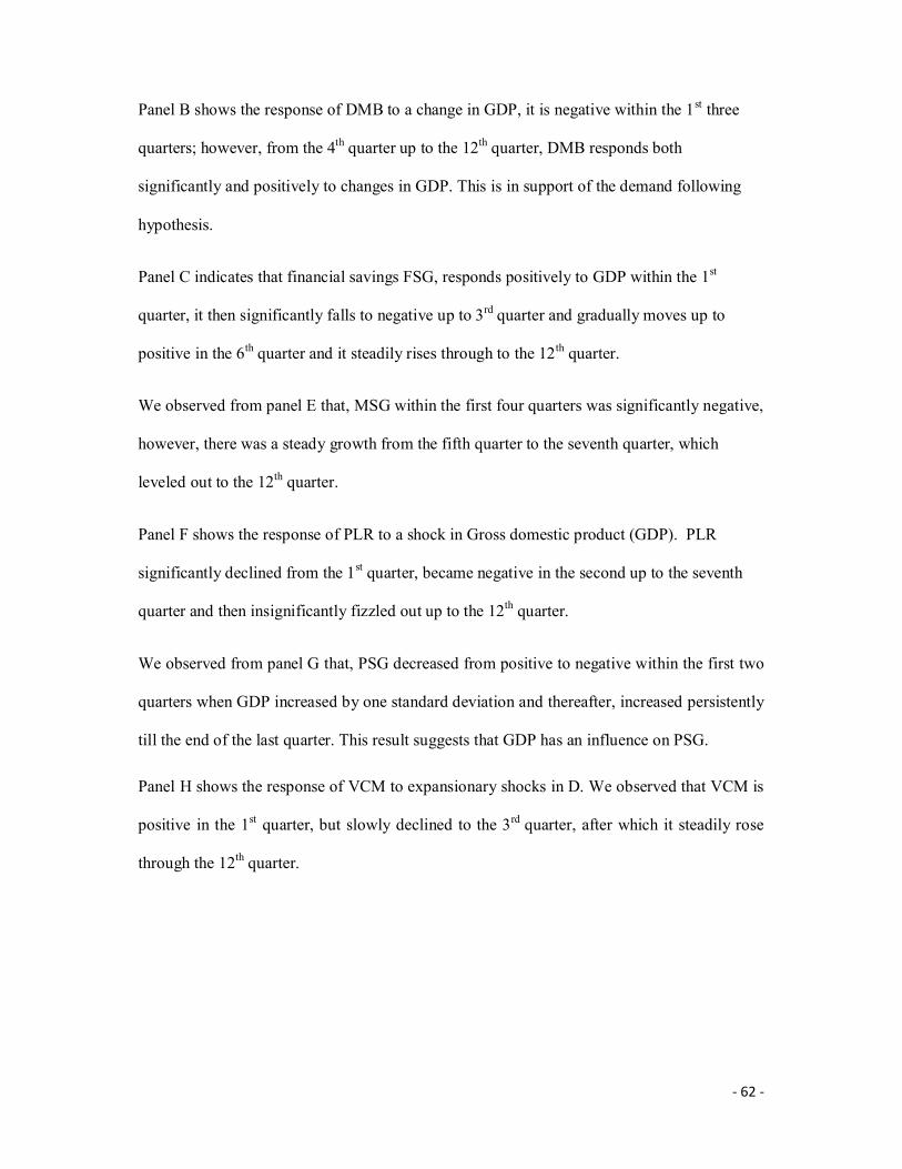
- 62 -

Panel B shows the response of DMB to a change in GDP, it is negative within the 1st three

quarters; however, from the 4th quarter up to the 12th quarter, DMB responds both

significantly and positively to changes in GDP. This is in support of the demand following

hypothesis.

Panel C indicates that financial savings FSG, responds positively to GDP within the 1st

quarter, it then significantly falls to negative up to 3rd quarter and gradually moves up to

positive in the 6th quarter and it steadily rises through to the 12th quarter.

We observed from panel E that, MSG within the first four quarters was significantly negative,

however, there was a steady growth from the fifth quarter to the seventh quarter, which

leveled out to the 12th quarter.

Panel F shows the response of PLR to a shock in Gross domestic product (GDP). PLR

significantly declined from the 1st quarter, became negative in the second up to the seventh

quarter and then insignificantly fizzled out up to the 12th quarter.

We observed from panel G that, PSG decreased from positive to negative within the first two

quarters when GDP increased by one standard deviation and thereafter, increased persistently

till the end of the last quarter. This result suggests that GDP has an influence on PSG.

Panel H shows the response of VCM to expansionary shocks in D. We observed that VCM is

positive in the 1st quarter, but slowly declined to the 3rd quarter, after which it steadily rose

through the 12th quarter.

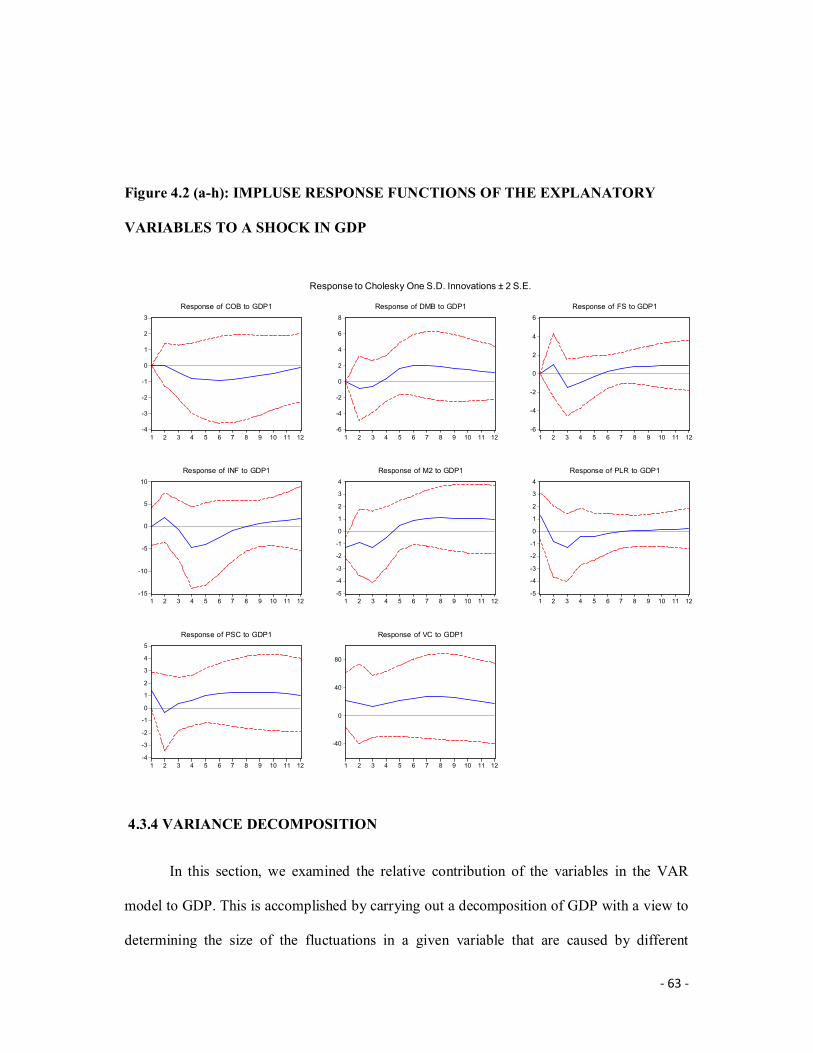
- 63 -

Figure 4.2 (a-h): IMPLUSE RESPONSE FUNCTIONS OF THE EXPLANATORY

VARIABLES TO A SHOCK IN GDP

4.3.4 VARIANCE DECOMPOSITION

In this section, we examined the relative contribution of the variables in the VAR

model to GDP. This is accomplished by carrying out a decomposition of GDP with a view to

determining the size of the fluctuations in a given variable that are caused by different

-4

-3

-2

-1

0

1

2

3

1 2 3 4 5 6 7 8 9 10 11 12

Response of COB to GDP1

-6

-4

-2

0

2

4

6

8

1 2 3 4 5 6 7 8 9 10 11 12

Response of DMB to GDP1

-6

-4

-2

0

2

4

6

1 2 3 4 5 6 7 8 9 10 11 12

Response of FS to GDP1

-15

-10

-5

0

5

10

1 2 3 4 5 6 7 8 9 10 11 12

Response of INF to GDP1

-5

-4

-3

-2

-1

0

1

2

3

4

1 2 3 4 5 6 7 8 9 10 11 12

Response of M2 to GDP1

-5

-4

-3

-2

-1

0

1

2

3

4

1 2 3 4 5 6 7 8 9 10 11 12

Response of PLR to GDP1

-4

-3

-2

-1

0

1

2

3

4

5

1 2 3 4 5 6 7 8 9 10 11 12

Response of PSC to GDP1

-40

0

40

80

1 2 3 4 5 6 7 8 9 10 11 12

Response of VC to GDP1

Response to Cholesky One S.D. Innovations ± 2 S.E.

- 64 -

shocks. We calculated the variance decomposition at forecast horizons from the first to the 10

quarters. The first to the fourth quarters represent the short run, while the eighth and 10

quarters represent the medium term.

Table 4.3 shows that, deposit money bank contributes more to GDP in the first three

quarters than the other variables and from the fourth quarter, the financial deepening variable

MSG contributes more significantly and relatively to GDP. For instance, in the third quarter,

DMB accounts for 7.5% of the variability in GDP. In the fourth, eighth and tenth quarter,

MSG accounts for 18.6%, 47.7% and 48.8% for the variations in GDP respectively.

However, the contribution of the private sector credit and prime lending rate to total GDP is

very small when compared with the other variables of financial development. This possibly

implies that a good percentage of the deposit money banks lending is not really to the private

sector but, rather to other areas of the economy.

Conclusively, our empirical findings point at a supply-leading hypothesis confirming the fact

financial deepening leads to economic growth in Nigeria.

Table 4.7: Variance Decomposition of GDP:

Period S.E. M2 PSC INF FS VC PLR DMB COB GDP

1.000 4.360 0.000 0.000 0.000 0.000 0.000 0.000 0.000 0.000 100.000

2.000 6.723 0.001 0.688 0.320 5.692 2.541 0.017 7.069 4.675 78.996

3.000 7.956 5.242 0.610 1.361 4.008 2.085 0.277 9.703 10.049 66.665

4.000 8.396 18.644 0.448 1.985 3.468 1.897 0.560 7.489 11.109 54.400

5.000 8.724 32.294 0.379 1.937 3.719 3.257 0.629 6.337 9.503 41.945

6.000 9.158 41.102 0.634 1.791 3.996 4.747 0.594 7.542 7.471 32.124

7.000 9.642 45.627 1.279 1.787 4.183 5.532 0.547 9.716 5.880 25.448

8.000 10.111 47.730 2.203 1.967 4.342 5.664 0.524 11.725 4.771 21.075

9.000 10.542 48.615 3.276 2.294 4.525 5.414 0.532 13.155 4.013 18.176

10.000 10.932 48.879 4.414 2.704 4.741 4.995 0.572 13.969 3.511 16.214

Source: Eviews software

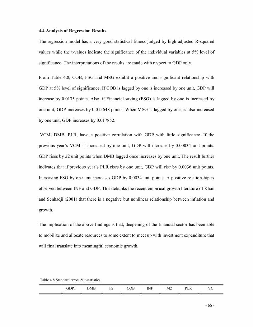
- 65 -

4.4 Analysis of Regression Results

The regression model has a very good statistical fitness judged by high adjusted R-squared

values while the t-values indicate the significance of the individual variables at 5% level of

significance. The interpretations of the results are made with respect to GDP only.

From Table 4.8, COB, FSG and MSG exhibit a positive and significant relationship with

GDP at 5% level of significance. If COB is lagged by one is increased by one unit, GDP will

increase by 0.0175 points. Also, if Financial saving (FSG) is lagged by one is increased by

one unit, GDP increases by 0.015648 points. When MSG is lagged by one, is also increased

by one unit, GDP increases by 0.017852.

VCM, DMB, PLR, have a positive correlation with GDP with little significance. If the

previous year’s VCM is increased by one unit, GDP will increase by 0.00034 unit points.

GDP rises by 22 unit points when DMB lagged once increases by one unit. The result further

indicates that if previous year’s PLR rises by one unit, GDP will rise by 0.0036 unit points.

Increasing FSG by one unit increases GDP by 0.0034 unit points. A positive relationship is

observed between INF and GDP. This debunks the recent empirical growth literature of Khan

and Senhadji (2001) that there is a negative but nonlinear relationship between inflation and

growth.

The implication of the above findings is that, deepening of the financial sector has been able

to mobilize and allocate resources to some extent to meet up with investment expenditure that

will final translate into meaningful economic growth.

Table 4.8 Standard errors & t-statistics

GDP1 DMB FS COB INF M2 PLR VC

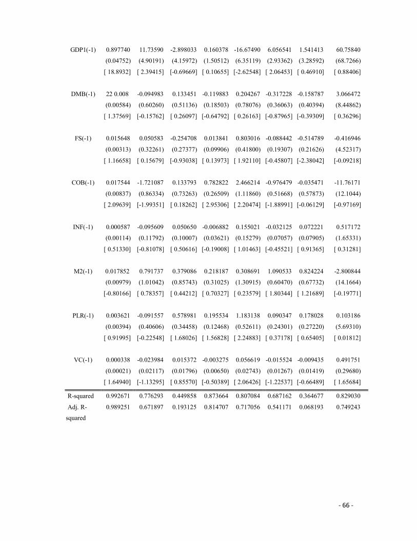
- 66 -

GDP1(-1) 0.897740 11.73590 -2.898033 0.160378 -16.67490 6.056541 1.541413 60.75840

(0.04752) (4.90191) (4.15972) (1.50512) (6.35119) (2.93362) (3.28592) (68.7266)

[ 18.8932] [ 2.39415] [-0.69669] [ 0.10655] [-2.62548] [ 2.06453] [ 0.46910] [ 0.88406]

DMB(-1) 22 0.008 -0.094983 0.133451 -0.119883 0.204267 -0.317228 -0.158787 3.066472

(0.00584) (0.60260) (0.51136) (0.18503) (0.78076) (0.36063) (0.40394) (8.44862)

[ 1.37569] [-0.15762] [ 0.26097] [-0.64792] [ 0.26163] [-0.87965] [-0.39309] [ 0.36296]

FS(-1) 0.015648 0.050583 -0.254708 0.013841 0.803016 -0.088442 -0.514789 -0.416946

(0.00313) (0.32261) (0.27377) (0.09906) (0.41800) (0.19307) (0.21626) (4.52317)

[ 1.16658] [ 0.15679] [-0.93038] [ 0.13973] [ 1.92110] [-0.45807] [-2.38042] [-0.09218]

COB(-1) 0.017544 -1.721087 0.133793 0.782822 2.466214 -0.976479 -0.035471 -11.76171

(0.00837) (0.86334) (0.73263) (0.26509) (1.11860) (0.51668) (0.57873) (12.1044)

[ 2.09639] [-1.99351] [ 0.18262] [ 2.95306] [ 2.20474] [-1.88991] [-0.06129] [-0.97169]

INF(-1) 0.000587 -0.095609 0.050650 -0.006882 0.155021 -0.032125 0.072221 0.517172

(0.00114) (0.11792) (0.10007) (0.03621) (0.15279) (0.07057) (0.07905) (1.65331)

[ 0.51330] [-0.81078] [ 0.50616] [-0.19008] [ 1.01463] [-0.45521] [ 0.91365] [ 0.31281]

M2(-1) 0.017852 0.791737 0.379086 0.218187 0.308691 1.090533 0.824224 -2.800844

(0.00979) (1.01042) (0.85743) (0.31025) (1.30915) (0.60470) (0.67732) (14.1664)

[-0.80166] [ 0.78357] [ 0.44212] [ 0.70327] [ 0.23579] [ 1.80344] [ 1.21689] [-0.19771]

PLR(-1) 0.003621 -0.091557 0.578981 0.195534 1.183138 0.090347 0.178028 0.103186

(0.00394) (0.40606) (0.34458) (0.12468) (0.52611) (0.24301) (0.27220) (5.69310)

[ 0.91995] [-0.22548] [ 1.68026] [ 1.56828] [ 2.24883] [ 0.37178] [ 0.65405] [ 0.01812]

VC(-1) 0.000338 -0.023984 0.015372 -0.003275 0.056619 -0.015524 -0.009435 0.491751

(0.00021) (0.02117) (0.01796) (0.00650) (0.02743) (0.01267) (0.01419) (0.29680)

[ 1.64940] [-1.13295] [ 0.85570] [-0.50389] [ 2.06426] [-1.22537] [-0.66489] [ 1.65684]

R-squared 0.992671 0.776293 0.449858 0.873664 0.807084 0.687162 0.364677 0.829030

Adj. R-

squared

0.989251 0.671897 0.193125 0.814707 0.717056 0.541171 0.068193 0.749243

- 67 -

CHAPETER FIVE

SUMMARY, CONCLUSION AND RECOMMENDATIONS

5.1 SUMMARY OF FINDINGS

The study empirically investigated the impact of financial deepening on economic

growth in Nigeria, with the view of determining which of the hypothesis (theories) is relevant

in the Nigerian economy, is it supply leading (Financial deepening leads to economic growth)

or demand following (economic growth triggers financial deepening). The literature on the

relationship between the economic growth and financial development overwhelmingly

suggest as positive, first-order relationship between the two. Nevertheless, empirical studies

on the issue of causality between the financial development and economic growth, however,

remain sparse (Pagano, 1993).

To represent economic growth, we used GDP (Gross domestic product) and

percentage change data natural logarithm was taken. Financial deepening was defined to

include MSG (the ratio of money supply to GDP, VCM (value of cheques to money supply),

PSG (ratio of private sector credit to GDP), FSG (financial savings to GDP), INF (rate of

inflation), PLR (real lending rates), DMB (deposit money bank assets to GDP), COB

(currency outside Banks to money supply). The prime lending rates of the banks was used to

stand for interest rate (the long term interest).

To attain the set objectives, we employed the Structural Vector Auto Regressive

method because it uses economic theory to sort out the links among the desired variables with

the standard practice reporting the Granger causality tests, impulse response functions and the

variance decompositions according to (Stock and Mark, 2001). But before employing the

VAR we investigated the nature of the time series data using both Augmented Dickey-Fuller

(ADF) and Philip Peron (PP) tests

- 68 -

Major findings

From the empirical analysis we found out that; financial deepening does not impact or

influence economic growth in the short run. However, in the long run there is a significant

effect of financial deepening on economic growth. Lending credence to the supply leading

hypothesis that financial deepening causes economic growth.

Also, the private sector credit contributes positively to economic growth; however,

the level of significance is very low. A positive relationship is observed between inflation and

GDP. This result is in line with the a priori expectations since we normally expect rising

inflationary pressures to have a positive effect on growth. Even though there has been clear

improvement in the financial sector over the past few decades, the degree of financial

development is still below the threshold needed to spur economic growth. The implication is

that the financial sector is still not able to mobilize and effectively allocate funds to the

private sector.

From the demand side, it was also observed that GDP had a positive and significant

impact on Deposit Money Bank Asset, Money supply and private sector credit, thereby

laying credence to the demand following hypothesis. In the Long-run, there is strong

evidence that economic growth is leading financial development when bank credit to private

sector is used thereby supporting the demand following hypothesis.

- 69 -

5.2 CONCLUSION

In this study, we used the structural vector auto-regressive (SVAR) model to

empirically analyze financial deepening and economic growth in Nigeria, given the two

theories; supply leading and demand following hypotheses. The study basically investigated

the causality between financial deepening and economic growth. Results showed that in

Nigeria some of the indicators of financial deepening; money supply, private sector credit,

inflation, favoured the supply leading hypothesis, meaning that financial deepening

influenced economic growth. The financial sector has an important role to play in the growth

of the Nigerian economy. We also observed some traces of demand following hypothesis

with financial deepening variables like private sector credit and deposit money banks

responding positively to gross domestic product. However, this study concluded that financial

deepening propels economic growth because the variables of financial deepening were more

significant in explaining economic growth, therefore supporting the supply leading

hypothesis.

5.3 RECOMMENDATIONS

There should be a determined effort by the monetary authorities to bridge the gap

existing between lending rate and deposit rate, foster a moderate rise in nominal rates and

stabilize inflationary pressures so that the people will be fully motivated to save in a bid to

generate needed loanable funds for investment in Nigeria. Savings must be encouraged and

any country that does not encourage savings should forget about making any investment,

whether private or public, (Fry, 1988).

There is an urgent need to sustain a higher level of macroeconomic stability in

Nigeria, reduce the high incidence of non performing credits ensure that private sector credits

are channeled to the real sector of the economy, enhance the level of corporate governance in

the financial system.

- 70 -

Based on the findings of the study, another recommendation is that monetary

authorities should continue with the policy reforms to consolidate the emerging confidence in

the financial system. The financial sector reforms should be intensified; this will create a

sound market-oriented financial sector, leading to an increase in the level of financial savings

and level of financial activities in the financial markets, which will translate to increased

deepening and hence economic growth.

The Central Bank of Nigeria should be encouraged with their current drive to ensure a

cashless economy. This will help to bring the currency outside banks to its lowest level since

everyone willing to carry out any transaction will need to have an account with one of the

financial institutions. Therefore, efforts should be made to extend financial services to the

informal or rural areas. There should be a decentralization of financial activities from the

urban areas to the rural areas.

DIRECTION OF RESEARCH

The findings in this study suggest there is much room for further study. While there exists, an

empirical link between financial development and economic growth, yet, there is still limited

knowledge on the support of the supply leading or demand following hypothesis in Nigeria.

Further analysis along these and similar lines appears a promising avenue for future research.

- 71 -

REFERENCES

Adebiyi, M.A. (2002): Is Financial Sector Liberalization the Cause of Banking Fragility in

Nigeria? African Review of Money, Finance and Banking, 23-40.

Aghion, P., Bacchetta, P., and Banerjee, A. (2004): Financial Development and Ang, J.B.

(2007). Financial Deepening and Economic Development in Malaysia.” Economic Papers, 26

(3), September, 249-260.

Ajayi, S.I. (2006). The Determinants of Foreign Direct Investment in Africa: A Survey of the

Evidence. In S.I Ajayi (Ed), Foreign Direct Investment in Sub-Saharan Africa: Origins,

Targets, Impact and Potential. Nairobi, Kenya: African Economic Research Consortium and

Insurance, Vol. 4, No 1. Pp. 46-67.

Ayida, O.E. (2007) Structural Adjustment, Financial Development and Economic Prosperity

in Nigeria, International Journal of Finance and Economics, Vol. 19. Central Bank of Nigeria

Annual Report and Accounts, Various Issues Statistical Bulletin, Various Issues.

Beck, T, Demirguc. K, Levine, R (2000a). A new database on financial development and

structure. World Bank Economic Review 14 (3), 597– 605.

Beck T, and Ross, L (1999): “A New Database on Financial Development and Structure,”

World Bank, unpublished.

Bencivenga, V.R. and Smith, B.D (1991): “Financial intermediation and endogenous

growth”. Review of Economic Studies, 58(2): 403–44.

Chang, T. and Caudill, S. B (2005): Financial development and economic growth: The case

of Taiwan, Applied Economics, 37, 1329-35.

Christopoulos, D. K. and Tsionas, E. G. (2004): Financial development and economic

growth: evidence from panel unit root and cointegration tests, Journal of Development

Economics, 73, 55-74.

- 72 -

Cletus C. A and Jude O. C. (2008): Toda and Yamamoto Causality Tests between “Bank-

Based” Financial Deepening and Economic Growth in Nigeria.

Cross-Country Comparisons”, In: Financial Structure and Economic Growth: A Cross-

Country Comparison of Banks, Markets, and Development, Eds: A. Demirguc-Kunt and R.

Levine. Cambridge, MA: MIT Press: 81-140. Delivered at National Institute for Policy and

Strategic Studies, August.

Demetriades, P.O. and Hussein, K.A. (1996). Does financial development cause economic

growth? Time series evidence from 16 countries, Journal of Development Economics, 51, pp.

387-411.

Demirgüç, K, and Ross, L (2001b): “Bank-Based and Market-Based Financial Systems:

Dong He and Robert Pardy (1993). “Stock Market Development and Financial Deepening in

Developing Countries: Some Correlation Patterns”, The World Bank, Policy Research

Working Paper 1084.

Felix, A et al (2008): Structural Adjustment, Financial Sector Development and Economic

Prosperity in Nigeria. International Research Journal of Finance and Economics ISSN 1450-

2887 Issue 15 (2008)

Ghani, E. 1992. “How financial markets affect long-run growth: A cross country study”.

World Bank Working Paper Series 843, Operations Evaluation Department, Washington,

D.C.

Granger, C.W.J (1988) Some Recent Development in a Concept of causality. Journal of

Econometrics 39, 199-211.t of

Gujarati D. N. (1995); Basic Econometrics, 4th edition, United State Military

Academy, West Point McGraw – Hill, Inc. 1995

Hemachandra W. M. (1999): Financial Deepening and its Implications on Savings and

Investments in Sri Lanka.

- 73 -

Jin, J. C. (2000) Openness and Growth: An Interpretation of Empirical Evidence from East

Asian countries, The Journal of International Trade and Economic Development, Vol.9,

No.1, pp.5-17

John, E. and Ndebbio, U (2004): Financial deepening, economic growth and development:

Evidence from selected sub-Saharan African countries. African Economic Research

Consortium, P.O. Box 62882-00200 Nairobi, Kenya

Journal of Economic Literature , Vol. 35, No. 2, pp. 688-726.

Khan and Mohsin (2002): Inflation, Financial Deepening, and Economic Growth. Conference

on Macroeconomic Stability, Financial Markets and Economic Development, Mexico City

Khan, S and Abdelhak, S (2000): “Financial Development and Economic Growth,” IMF

Working Paper WP/00/209; Journal of African Economies, forthcoming.

King, R.G. and Levine, R (1993): “Finance, entrepreneurship and growth: Theory and

evidence”. Journal of Monetary Economics, 32(3): 513–542.

Levine, R (1997): “Financial Development and Economic Growth: Views and Agenda,”

Luintel, K.B. and Khan, M., (1999), A Quantitative Reassessment of the Finance Growth

Nexus: Evidence from a Multivariate VAR , Journal of Development Economics, 60, 381-

405

Manning, M. J (2003): “Finance Causes Growth: Can We Be So Sure?” Contributions to

Macroeconomics, 3 (2003), http://www.bepress.com/bejm/contributions/vol3/iss1/art12

Michael, A (2003): A Re-examination of McKinnon-Shaw Financial Development

Hypotheses: Evidence from Seven African Countries. The Nigerian Journal of Risk

Montiel, P.J. 1995. “Financial policies and economic growth: Theory, evidence, and country-

specific experience from sub-Saharan Africa”. AERC Special Paper (April 1995).

Nagel, A and Jeffrey P (2003): “Empirical macroeconomics: The effects of monetary policy”.

Paper Presented at the Gold-Hammer Collaborative Research at Reed College.

- 74 -

Ndebbio, J.E. (2004) Financial Deepening, Economic Growth and Development: Evidence

from Selected Sub-Sahara African Countries, AERC Research Papers No. 142 African

Economic Research Consortium, Naira.

Nicholas, A et’al (2007) Financial Deepening and Economic Growth Linkages: A Panel Data

Analysis, University of Piraeus, Piraeus; Utrecht School of Economics, University of Utrecht.

Review of World Economics 2007, Vol. 143 (1)

Nnanna, O (2001): “Monetary Management: Objectives, Tools and the Role of Central Banks

in the Region”. Regional Forum on Economic and Financial Management for

Parliamentarians. Nigeria:WAIFEM.

Ogun, O.D. (1986) A Note on Financial Deepening and Economic Growth: Evidence from

Africa, Nigerian Journal of Economic and Social Studies,28 (2).

Ogun, O.D. (1986): “A note on financial deepening and economic growth: Evidence from

Africa”. The Nigerian Journal of Economic and Social Studies, 28(2): 275–283.

Olofin, S. et’al (2008) Financial Structure and Economic Growth in Nigeria, Nigerian Journal

of Securities and Finance Vol. 13 No. 1 Pp 47-68 Oloyide, A. (1998). The Financial Systems

Role in Resource Mobilization and investment: An Analysis of Financial Deepening in

Nigeria’s Financial Sector, Economic and Financial Review, Abuja.

Ozturk, I et’al (2007): Finance – Growth Nexus: Evidence From Turkey.” International

Research Journal of Finance and Economics, 11, 30-40. [3]

Patrick, H (1966): Financial Development and Economic Growth in Underdeveloped

Countries, Economic Development and Culture Change Vol. 14 No. 2 Jan.

Peter, L and Rousseau (2007): What is happening to the impact of financial deepening on

economic growth?

- 75 -

Rao, M et’al (2010): Trade Liberalisation, Financial Development and Economic Growth:

Evidence from Pakistan (1980-2009). Journal of International Academic Research (2010)

Vol.10, No.2. 31 August 2010

Rudra, P. P (2010): Financial Deepening, Foreign Direct Investment and Economic Growth:

Are They Cointegrated. International Journal of Financial Research Vol. 1, No. 1; December

2010

Sam, Q. Z (2001): The Impact of Financial Sector Reform on Bank Efficiency and Financial

Deepening for Savings Mobilization in Ghana African Economic Policy Discussion Paper

Number 81 February 2001

Samuel, M. N and Emeka, J. O (2009): Financial deepening and economic evelopment of

Nigeria: an empirical investigation. African Journal of Accounting, Economics, Finance and

Banking Research Vol. 5. No. 5

Sanusi, J.O. (2002b): Central bank and the Macroeconomic Environment in Nigeria.” Lecture

Shaw, E (1973): Financial Deepening in Economic Development, London, Oxford University

Press.

Sinkey, J. R. (1989): “Bank Financial Management in the Financial Services

Industry,” Macmillian Publishing Company.

Tabi, A. J et’al (2011): Financial development and economic growth in Cameroon, 1970-

2005. Journal of Economics and International Finance Vol. 3(6), pp. 367-375, June 2011

Thomas, G et’al (2008): Financial Deepening, Trade Openness and Economic Growth in

Latin America and the Caribbean. Center for International Economics University of

Paderborn, Warburger Strasse 100 33098 Paderborn / Germany.

Thornton, J (1995): “Financial Deepening and Economic Growth in Developing Countries,”

Economia Internazionale.

- 76 -

Valerie, R. B and Buce, D. S (1991): Financial Intermediation and Endogenous Growth.

Cornell University and Cornell University and Rochester Center for Economic Research

Yan, E. (2007): Why Isn't Financial Deepening Happening in Developing Countries,

www.worldbank.org.

Yucel, F. (2009): Causal Relationships between Financial Development, Trade Openness and

Economic Growth: The Case of Turkey, Journal of Social Sciences 5(1): 33-42, 2009.

- 77 -

APPENDICES

Variance Decomposition of GDP:

Period S.E. M2 PSC INF FS VC PLR DMB COB GDP1

1.0000 4.3597 0.0000 0.0000 0.0000 0.0000 0.0000 0.0000 0.0000 0.0000 100.0000

2.0000 6.7234 0.0008 0.6880 0.3205 5.6923 2.5408 0.0173 7.0694 4.6753 78.9956

3.0000 7.9556 5.2421 0.6100 1.3609 4.0080 2.0855 0.2768 9.7031 10.0486 66.6650

4.0000 8.3964 18.6442 0.4485 1.9849 3.4678 1.8967 0.5600 7.4887 11.1089 54.4003

5.0000 8.7240 32.2945 0.3792 1.9370 3.7186 3.2575 0.6288 6.3373 9.5027 41.9445

6.0000 9.1583 41.1017 0.6337 1.7914 3.9964 4.7466 0.5937 7.5418 7.4711 32.1235

7.0000 9.6425 45.6274 1.2788 1.7871 4.1829 5.5320 0.5471 9.7164 5.8804 25.4480

8.0000 10.1113 47.7298 2.2032 1.9667 4.3419 5.6641 0.5238 11.7252 4.7706 21.0748

9.0000 10.5424 48.6150 3.2758 2.2937 4.5251 5.4140 0.5321 13.1546 4.0134 18.1763

10.0000 10.9324 48.8793 4.4144 2.7045 4.7406 4.9947 0.5723 13.9692 3.5111 16.2141

Variance Decomposition of M2:

Period S.E. M2 PSC INF FS VC PLR DMB COB GDP1

1.0000 6.3949 30.9642 0.0000 0.0000 0.0000 0.0000 0.0000 0.0000 0.0000 69.0358

2.0000 7.3201 36.5923 1.5122 0.0045 8.8984 4.4038 1.0815 6.0976 2.4244 38.9853

3.0000 7.8374 31.0981 2.2695 0.0046 10.1360 4.6988 0.8722 11.9859 7.6130 31.3219

4.0000 8.3847 27.9263 4.9389 0.0061 9.2321 4.2356 0.7916 13.0349 11.2640 28.5706

5.0000 9.0550 26.7712 7.1611 0.1442 8.5538 5.4179 0.7827 12.0810 12.4008 26.6874

6.0000 9.7852 25.9880 7.8275 0.3900 7.7812 7.7488 0.8230 12.3283 12.1401 24.9732

7.0000 10.5286 25.1195 7.6034 0.5209 7.0407 9.9357 0.8957 14.2181 11.4016 23.2645

8.0000 11.2486 24.2440 7.0951 0.5256 6.4263 11.4722 0.9675 16.9539 10.6328 21.6826

9.0000 11.9138 23.4643 6.5704 0.4858 5.9489 12.4097 1.0154 19.8585 9.9370 20.3099

10.0000 12.4981 22.7979 6.1131 0.4591 5.5937 12.9206 1.0361 22.5965 9.3156 19.1675

Variance Decomposition of PSC:

Period S.E. M2 PSC INF FS VC PLR DMB COB GDP1

1.0000 10.4080 16.9429 69.1277 0.0000 0.0000 0.0000 0.0000 0.0000 0.0000 13.9295

2.0000 13.0606 13.1800 62.7438 0.0261 0.0788 0.0185 0.1570 5.4018 6.6492 11.7449

3.0000 18.8829 11.7309 58.9898 1.1872 0.8559 1.9827 0.3664 4.9421 9.4544 10.4909

4.0000 24.1785 12.0944 54.2577 1.5560 0.7612 5.4068 0.5032 4.8392 11.0626 9.5189

5.0000 27.3878 12.8799 48.0403 1.6695 0.6532 9.1281 0.6798 7.1301 10.9923 8.8267

6.0000 28.9759 13.6716 41.7593 1.5584 0.5749 11.9998 0.8223 11.1070 10.3200 8.1868

7.0000 29.7396 14.3173 36.2798 1.3645 0.5510 13.8484 0.9082 15.7137 9.4317 7.5854

8.0000 30.1906 14.7795 31.8255 1.1969 0.5852 14.8640 0.9447 20.2152 8.5185 7.0705

9.0000 30.5608 15.0614 28.3707 1.0941 0.6679 15.2912 0.9467 24.2203 7.6893 6.6585

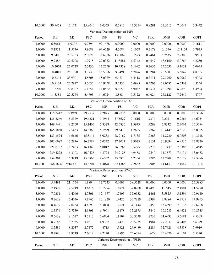
- 78 -

10.0000 30.9458 15.1741 25.8040 1.0563 0.7813 15.3354 0.9291 27.5712 7.0044 6.3442

Variance Decomposition of INF:

Period S.E. M2 PSC INF FS VC PLR DMB COB GDP1

1.0000 6.5061 6.9307 0.7594 92.1488 0.0000 0.0000 0.0000 0.0000 0.0000 0.1611

2.0000 8.1921 11.5046 5.9689 64.6229 4.5084 0.1058 0.2178 0.1656 12.1124 0.7935

3.0000 9.3408 29.5763 2.9020 35.6726 13.0069 3.1523 0.7461 6.7635 7.2300 0.9503

4.0000 9.9386 29.5008 1.7915 22.0332 11.8581 6.5342 0.4647 18.5160 5.0766 4.2250

5.0000 10.2074 27.0728 2.2430 17.2259 10.4328 7.1692 0.3657 25.2631 5.1631 5.0645

6.0000 10.4018 25.1720 3.3733 15.5386 9.7491 6.7826 0.3284 28.5007 5.6847 4.8705

7.0000 10.6343 23.9901 4.5608 15.0379 9.4234 6.4418 0.3131 29.3960 6.2062 4.6308

8.0000 10.9134 23.2877 5.5033 14.9358 9.2333 6.4985 0.3207 29.0587 6.6367 4.5254

9.0000 11.2200 22.8387 6.1254 14.8622 9.0659 6.9037 0.3534 28.3694 6.9890 4.4924

10.0000 11.5381 22.5274 6.4703 14.6724 8.8684 7.5122 0.4024 27.8122 7.2640 4.4707

Variance Decomposition of FS:

Period S.E. M2 PSC INF FS VC PLR DMB COB GDP1

1.0000 115.2417 0.3969 29.9537 2.2875 40.9733 0.0000 0.0000 0.0000 0.0000 26.3886

2.0000 135.3269 15.8379 19.6221 7.1964 37.5629 0.1616 1.7374 0.2021 0.9864 16.6934

3.0000 149.5471 18.2760 15.1465 5.8528 32.5836 1.5943 1.4298 6.8332 2.7063 15.5774

4.0000 165.1838 17.5433 14.6360 5.1929 29.5470 1.7685 1.2762 10.4149 4.6128 15.0085

5.0000 183.1574 16.6646 15.5114 5.0233 28.2169 1.7135 1.2263 11.2720 6.0603 14.3118

6.0000 202.6087 16.2846 16.2789 5.0242 27.2014 2.3023 1.2151 10.9094 6.9515 13.8326

7.0000 221.8787 16.2463 16.4340 5.0012 26.0265 3.5275 1.2276 10.7439 7.3385 13.4545

8.0000 239.4222 16.3103 16.0528 4.8724 24.7128 4.9488 1.2540 11.3873 7.4134 13.0482

9.0000 254.3011 16.3849 15.3865 4.6552 23.3870 6.2354 1.2786 12.7708 7.3129 12.5886

10.0000 266.1626 **16.4510 14.6204 4.4078 22.1365 7.2632 1.2905 14.6153 7.1049 12.1104

Variance Decomposition of VC:

Period S.E. M2 PSC INF FS VC PLR DMB COB GDP1

1.0000 5.4491 21.1754 1.8894 12.7245 0.0693 38.5528 0.0000 0.0000 0.0000 25.5885

2.0000 7.1992 17.5249 3.6316 13.7294 1.6724 37.8208 0.7490 1.1645 2.1804 21.5270

3.0000 7.9251 16.4066 4.7501 12.1977 1.7405 37.0532 1.1461 3.5825 5.1594 17.9640

4.0000 8.2628 16.4036 5.1945 10.1820 1.4425 35.7819 1.3399 7.8884 6.7717 14.9955

5.0000 8.4699 17.0254 4.8599 8.3088 1.2021 34.1144 1.3853 13.4699 7.0135 12.6208

6.0000 8.5874 17.7259 4.1801 6.7901 1.1178 32.2175 1.3449 19.3283 6.4621 10.8335

7.0000 8.6638 18.1627 3.5113 5.6804 1.1504 30.3039 1.2737 24.6993 5.6681 9.5503

8.0000 8.7185 18.2955 3.0219 4.9337 1.2429 28.5235 1.1984 29.2037 4.9405 8.6399

9.0000 8.7589 18.2037 2.7472 4.4713 1.3621 26.9489 1.1286 32.7625 4.3838 7.9919

10.0000 8.7890 17.9749 2.6618 4.2170 1.4896 25.6094 1.0679 35.4370 4.0104 7.5320

Variance Decomposition of PLR:

Period S.E. M2 PSC INF FS VC PLR DMB COB GDP1

- 79 -

1.0000 8.1568 35.1001 0.4873 3.3790 19.6339 18.7546 19.4608 0.0000 0.0000 3.1844

2.0000 10.0562 34.5360 6.5502 4.6192 25.2740 13.9415 11.3420 1.3210 0.0376 2.3786

3.0000 10.7724 31.8332 5.4053 4.5283 20.8574 14.8562 9.4394 6.3949 0.4439 6.2413

4.0000 11.4754 31.6050 5.1975 4.1691 19.4898 15.0550 8.6884 9.2396 0.4421 6.1134

5.0000 12.6464 30.9962 5.1600 3.9874 18.6723 14.8888 8.2814 11.6067 0.5087 5.8985

6.0000 13.9858 30.5797 5.3253 3.9583 18.2218 14.6278 8.0597 12.9425 0.5456 5.7393

7.0000 15.1767 30.3159 5.5164 4.0285 17.9724 14.3945 7.9183 13.6306 0.5767 5.6465

8.0000 16.1221 30.1317 5.6957 4.1229 17.8291 14.2149 7.8231 13.9706 0.6253 5.5868

9.0000 16.8416 29.9824 5.8716 4.2052 17.7428 14.0890 7.7602 14.1032 0.6999 5.5457

10.0000 17.3783 29.8416 6.0450 4.2682 17.6824 14.0174 7.7205 14.1070 0.7972 5.5208

Variance Decomposition of DMB:

Period S.E. MSG PSC INF FSG VCM PLR DMB COB GDP

1.0000 2.4164 20.0541 5.6230 0.6009 0.0618 1.4658 0.2111 19.0523 0.0000 52.9309

2.0000 3.4080 20.9873 6.1207 1.9163 2.7936 1.9995 1.3286 12.6312 6.4214 45.8013

3.0000 4.6583 18.5993 6.6318 1.8481 4.3477 1.7496 1.4324 11.0896 12.9100 41.3916

4.0000 5.9472 18.7294 7.9094 1.7943 3.9478 3.4070 1.3166 10.6332 15.7854 36.4769

5.0000 7.1301 19.8559 7.7223 1.4781 3.6246 7.1704 1.1963 13.7887 14.1786 30.9852

6.0000 8.1500 20.1526 6.5898 1.2249 3.2700 10.2396 1.1255 18.9213 11.8749 26.6015

7.0000 8.9881 19.7876 5.6106 1.0406 2.9946 11.8807 1.0961 23.9706 10.1445 23.4749

8.0000 9.6533 19.2227 4.9888 0.9391 2.8190 12.5239 1.0780 28.1138 8.9979 21.3168

9.0000 10.1633 18.6782 4.6472 0.9246 2.7322 12.6363 1.0556 31.2455 8.2458 19.8347

10.0000 10.5381 18.2028 4.4919 0.9737 2.7111 12.5037 1.0286 33.5064 7.7584 18.8235

Variance Decomposition of COB:

Period S.E. MSG PSC INF FSG VCM PLR DMB COB GDP

1.0000 0.0780 0.1994 11.7084 3.0420 23.4584 2.3036 12.2551 0.7668 45.1962 1.0702

2.0000 0.1137 9.0123 8.5755 2.0067 13.2517 12.4176 6.9850 6.3041 40.6951 0.7519

3.0000 0.1421 19.3005 6.9377 1.1105 7.7815 17.7748 4.0208 14.7893 27.8117 0.4730

4.0000 0.1657 23.1183 4.7768 0.6825 5.2597 20.0059 2.7284 23.7101 18.6426 1.0758

5.0000 0.1919 24.5172 3.3400 0.5055 4.1893 20.2139 2.0636 30.3051 13.4749 1.3906

6.0000 0.2210 24.7849 2.6021 0.4892 3.7218 19.5659 1.6827 35.2320 10.4316 1.4898

7.0000 0.2503 24.6217 2.3382 0.5889 3.5351 18.6040 1.4405 38.8045 8.5862 1.4809

8.0000 0.2779 24.3125 2.3846 0.7714 3.5059 17.5795 1.2739 41.2932 7.4515 1.4275

9.0000 0.3034 23.9525 2.6364 1.0024 3.5651 16.6173 1.1564 42.9273 6.7794 1.3632

10.0000 0.3267 23.5756 3.0267 1.2532 3.6670 15.7834 1.0760 43.8814 6.4355 1.3012

Cholesky Ordering: GDP1 M2 PSC INF FS VC PLR DMB COB

- 80 -

Vector Autoregression Estimates

Date: 11/05/11 Time: 11:55

Sample(adjusted): 1987 2009

Included observations: 23 after adjusting endpoints

Standard errors in ( ) & t-statistics in [ ]

GDP1 DMB FSG COB INF MSG PLR VCM

GDP1(-1) 0.897740 11.73590 -2.898033 0.160378 -16.67490 6.056541 1.541413 60.75840

(0.04752) (4.90191) (4.15972) (1.50512) (6.35119) (2.93362) (3.28592) (68.7266)

[ 18.8932] [ 2.39415] [-0.69669] [ 0.10655] [-2.62548] [ 2.06453] [ 0.46910] [ 0.88406]

DMB(-1) 0.008036 -0.094983 0.133451 -0.119883 0.204267 -0.317228 -0.158787 3.066472

(0.00584) (0.60260) (0.51136) (0.18503) (0.78076) (0.36063) (0.40394) (8.44862)

[ 1.37569] [-0.15762] [ 0.26097] [-0.64792] [ 0.26163] [-0.87965] [-0.39309] [ 0.36296]

FS(-1) 0.003648 0.050583 -0.254708 0.013841 0.803016 -0.088442 -0.514789 -0.416946

(0.00313) (0.32261) (0.27377) (0.09906) (0.41800) (0.19307) (0.21626) (4.52317)

[ 1.16658] [ 0.15679] [-0.93038] [ 0.13973] [ 1.92110] [-0.45807] [-2.38042] [-0.09218]

COB(-1) 0.017544 -1.721087 0.133793 0.782822 2.466214 -0.976479 -0.035471 -11.76171

(0.00837) (0.86334) (0.73263) (0.26509) (1.11860) (0.51668) (0.57873) (12.1044)

[ 2.09639] [-1.99351] [ 0.18262] [ 2.95306] [ 2.20474] [-1.88991] [-0.06129] [-0.97169]

INF(-1) 0.000587 -0.095609 0.050650 -0.006882 0.155021 -0.032125 0.072221 0.517172

(0.00114) (0.11792) (0.10007) (0.03621) (0.15279) (0.07057) (0.07905) (1.65331)

[ 0.51330] [-0.81078] [ 0.50616] [-0.19008] [ 1.01463] [-0.45521] [ 0.91365] [ 0.31281]

M2(-1) -0.007852 0.791737 0.379086 0.218187 0.308691 1.090533 0.824224 -2.800844

(0.00979) (1.01042) (0.85743) (0.31025) (1.30915) (0.60470) (0.67732) (14.1664)

[-0.80166] [ 0.78357] [ 0.44212] [ 0.70327] [ 0.23579] [ 1.80344] [ 1.21689] [-0.19771]

PLR(-1) 0.003621 -0.091557 0.578981 0.195534 1.183138 0.090347 0.178028 0.103186

(0.00394) (0.40606) (0.34458) (0.12468) (0.52611) (0.24301) (0.27220) (5.69310)

[ 0.91995] [-0.22548] [ 1.68026] [ 1.56828] [ 2.24883] [ 0.37178] [ 0.65405] [ 0.01812]

VC(-1) 0.000338 -0.023984 0.015372 -0.003275 0.056619 -0.015524 -0.009435 0.491751

(0.00021) (0.02117) (0.01796) (0.00650) (0.02743) (0.01267) (0.01419) (0.29680)

[ 1.64940] [-1.13295] [ 0.85570] [-0.50389] [ 2.06426] [-1.22537] [-0.66489] [ 1.65684]

R-squared 0.992671 0.776293 0.449858 0.873664 0.807084 0.687162 0.364677 0.829030

Adj. R-squared 0.989251 0.671897 0.193125 0.814707 0.717056 0.541171 0.068193 0.749243

- 81 -

Sum sq. resids 0.088969 946.8448 681.8292 89.26723 1589.489 339.1205 425.4635 186121.7

S.E. equation 0.077015 7.944997 6.742053 2.439498 10.29397 4.754791 5.325808 111.3917

F-statistic 290.2418 7.436011 1.752243 14.81869 8.964858 4.706877 1.230004 10.39063

Log likelihood 31.24649 -75.38846 -71.61236 -48.23120 -81.34583 -63.58049 -66.18896 -136.1202

Akaike AIC -2.021434 7.251170 6.922814 4.889669 7.769203 6.224390 6.451214 12.53219

Schwarz SC -1.626479 7.646125 7.317769 5.284624 8.164157 6.619345 6.846169 12.92715

Mean dependent 6.361304 38.55783 12.81130 24.36435 22.23913 25.68652 20.07174 257.4457

S.D. dependent 0.742828 13.87039 7.505665 5.667229 19.35233 7.019496 5.517247 222.4470

BS GDP COB DMB FSG INF MSG PLR PSC VC

1986 4.840 20.900 57.230 20.150 5.400 35.900 10.500 25.100 100.000

1987 5.020 21.000 47.000 17.790 10.200 28.600 17.500 18.800 89.000

1988 5.140 23.600 42.600 16.700 38.300 28.000 16.500 16.700 141.000

1989 5.340 18.000 30.200 11.000 40.900 21.300 26.800 14.300 84.500

1990 5.430 23.000 31.000 11.000 7.500 24.300 25.500 13.700 67.100

1991 5.490 26.800 37.600 12.000 13.000 27.600 20.010 14.500 96.800

1992 5.730 28.500 23.900 10.300 44.500 24.200 29.800 14.300 85.750

1993 5.830 29.140 33.000 12.400 57.200 29.000 36.030 13.300 103.500

1994 5.950 33.900 32.800 40.600 57.000 29.700 21.000 16.100 116.200

1995 6.290 33.590 20.000 5.600 72.800 16.500 10.180 10.600 126.000

1996 6.430 31.360 17.000 5.000 20.300 13.700 19.740 9.500 146.400

1997 6.450 30.400 20.000 6.300 8.500 15.300 13.540 11.300 96.400

1998 6.430 29.800 25.600 7.400 10.000 19.400 18.290 13.690 74.600

1999 6.500 26.690 33.500 8.600 6.600 21.900 21.320 14.200 171.300

2000 6.660 26.690 34.600 8.500 6.900 22.800 17.980 12.900 202.300

2001 6.670 25.740 47.950 10.400 18.900 28.100 18.290 17.700 171.500

2002 6.730 24.220 51.200 11.000 12.900 29.600 24.400 17.700 145.400

2003 6.840 20.800 43.900 9.400 14.000 28.100 20.480 17.400 449.800

2004 6.850 20.300 53.000 11.300 15.000 32.000 19.150 21.700 485.800

2005 7.160 21.400 31.300 9.000 17.900 18.000 17.850 13.800 747.800

2006 7.270 18.800 41.150 12.100 8.500 22.000 17.330 25.600 480.100

2007 7.320 15.200 61.700 18.000 6.600 29.400 16.460 48.000 584.000

2008 7.390 16.250 61.750 16.950 11.600 37.720 15.140 33.170 658.000

2009 7.390 15.200 66.080 23.320 12.400 43.570 18.360 41.300 598.000

Source Derived from Central Bank of Nigeria Statistical Bulletin 2010

- 82 -

Year GDP @curt price Fin Sav Inflation

Money supply

Private sectorCR

Deposit moni bnk

Curency O B

Prime L

1986 69,147.0 13,934.1 5.4 27,389.8

18,299.9 39,678.8 5,178

10.50

1987 105,222.8 18,676.3 10.2 33,667.4

21,892.5 49,828.4 6,299

17.50

1988 139,085.3 23,249.0 56.0 45,446.9

25,472.5 58,027.2 9,413

16.50

1989 216,797.5 23,801.3 50.5 47,055.0

29,643.9 64,874.0 11,688

26.80

1990 267,550.0 29,651.2 7.5 68,662.5

35,436.6 82,957.8 14,941

25.50

1991 312,139.7 37,738.2 12.7 87,499.8

42,079.0 117,511.9 23,108

20.01

1992 532,613.8 55,116.8 44.8 129,085.5

79,958.9 159,190.8 36,755

29.80

1993 683,869.8 85,027.9 57.2 198,479.2

95,529.7 226,162.8 57,845

36.03

1994 899,863.2 108,460.5 57.0 266,944.9

151,000.3 295,033.2 90,601

21.00

1995 1,933,211.6 108,490.3 72.8 318,763.5

211,358.6 385,141.8 106,843

10.18

1996 2,702,719.1 134,503.2 29.3 370,333.5

260,613.5 458,777.5 116,121

19.74

1997 2,801,972.6 177,648.7 10.7 429,731.3

319,512.2 584,375.0 130,668

13.54

1998 2,708,430.9 200,065.1 7.9 525,637.8

372,574.1 694,615.1 156,716

18.29

1999 3,194,015.0 277,667.5 6.6 699,733.7

455,205.2 1,070,019.8 186,456

21.32

2000 4,582,127.3 385,190.9 6.9 1,036,079.5

596,001.5 1,568,838.7 274,010

17.98

2001 4,725,086.0 488,045.4 18.9 1,315,869.1

854,999.3 2,247,039.9 338,671

18.29

2002 6,912,381.3 592,094.0 12.9 1,599,494.6

955,762.1 2,766,880.3 386,942

24.40

2003 8,487,031.6 655,739.7 14.0 1,985,191.8

1,211,993.4 3,047,856.3 412,155

20.48

2004 11,411,066.9 797,517.2 15.0 2,263,587.9

1,534,447.8 3,753,277.8 458,586

19.15

2005 14,572,239.1 1,316,957.4 17.8 2,814,846.1

2,007,355.8 4,515,117.6 563,232

17.85

2006 18,564,594.7 1,739,636.9 8.2 4,027,901.7

2,650,821.5 7,172,932.1 779,120

17.33

2007 20,657,317.7 2,693,554.3 5.4 5,809,826.5

5,056,720.9 10,981,693.6 960,000

16.46

2008 24,296,329.3 4,118,172.8 11.6 9,166,835.3

8,059,548.9 14,999,508.0

15.14

2009 24,712,669.9

5,763,511.2 12.4 10,767,377.8

10,206,086.7 16,329,218.5

18.36

Central Bank of Nigeria, Statistical Bulletin, Vol. 16 Dec. 2010

- 83 -