An Empirical Analysis for Determinants of Interest Rate ...

An Empirical Analysis for

Determinants of Interest Rate

Swap Spread

Master thesis for Finance program

Ke Zhang and Bing Liang

Economics Department University of Lund

May 28, 2007

An Empirical Analysis for Determinants of Interest Rate Swap Spread

of 43

Abstract As one of the most popular derivatives to hedge interest rate risk, the variation of interest

rate swap spread has been studied since its advent. Nevertheless, the variables in theory

are regarded as determinant risk factors showing limited explanatory power. To

investigate further, we conducted the cointegration test on each pair of variables which

are considered in the financial and macroeconomic sense, and extend the classic

Generalized Autoregressive Conditionally Heteroscedastic (GARCH) model by

combining the Error correction model (ECM). Our testing results suggest that the changes

in the swap spread negatively correlated with the slope of the yield curves of Treasury

Securities and positively correlated with the implied volatility of Stock market, while

other assumed determinant variables having a vague or even rather weak impact on the

swap spread in general.


of 43

Table of contents Abstract...........................................................................................................................2 1. Introduction.................................................................................................................4

1.1 Background ...........................................................................................................4 1.2 Limitations of previous discussions........................................................................4 1.3 The objective of this research.................................................................................5 1.4 Disposition of this paper ........................................................................................6

2. Literature Review ........................................................................................................7 2.1 Essentials of interest rate swap...............................................................................7 2.2 Mechanics of interest rate swap .............................................................................8 2.3 Theoretical determinants of interest rate swap spread.............................................8 2.4 Empirical researches ..............................................................................................9

3. Data Description........................................................................................................12 3.1 Sources of data ....................................................................................................12 3.2 Dependent variable ..............................................................................................16 3.3 Independent variables ..........................................................................................17

4. Methodology .............................................................................................................21 4.1 Empirical hypothesis............................................................................................21 4.2 Test procedures....................................................................................................22 4.3 GARCH model ....................................................................................................23 4.4 Cointegration model ............................................................................................25 4.5 GARCH with Error Correction Terms Model (ECT)............................................25

5. Empirical findings .....................................................................................................27 5.1 ADF Unit root test results ....................................................................................27 5.2 GARCH analysis .................................................................................................28 5.3 Cointegration analysis..........................................................................................29 5.4 Analysis of GARCH with Error Correction Terms ...............................................29 5.5 Hypothesis Test Results .......................................................................................30

6. Conclusions ...............................................................................................................35 7. Acknowledgements ...................................................................................................37 8. Appendix...................................................................................................................38 9. References.................................................................................................................41


of 43

1. Introduction We present our introduction as follows: background of interest rate swap, limitations of

previous discussions, objective of this research and disposition of our paper.

1.1 Background

An interest rate defines the amount of money a borrower promises to pay the lender.

There are many different types of regularly quoted interest rates which include mortgage

rates, deposit rates, prime borrowing rates, and so on. The application of the interest rate

relies on the credit risk since the higher the credit risk is, the higher the interest rate that is

promised by the borrower is. A large number of empirical researches show that interest

rate swaps are one of the major financial innovations since 1980s and the most popular

derivative contracts used by U.S. firms (In, Brown and Fang, 2003). The interest rate

swap market is one of the most important fixed-income markets in the trading and

hedging of interest risk. According to Bank for International Settlement (BIS) statistics

results on the notional amounts outstanding in the OTC Derivatives market, the total

trading has reached USD 248,288 billion, which equals to six times world GDP at the end

of 2004. The majority of this trading (USD 147.4 trillion) was interest rate swaps (Bank

for International Settlement, 2005).

1.2 Limitations of previous discussions

The previous empirical research about the interest swap spread is what determines

interest rate swap spreads and new findings why the interest rate swap spread fluctuate so

much. Based on the previous research, we can see that the literature on swap spread

focuses on the following factors: interest rate, credit risk, liquidity and default rate.

Litezenberger (1992) and Turnbull (1987) showed that the most standard model in the

interest rate swap market is to equal the present values of the cash flows arising from the

fixed-rate side and the floating-rate side. In order to solve for the swap rate, Sorensen and

Billier (1994) argue that the interest rate swap can be explained by using the option


of 43

pricing model since the credit risk between two counter-parties is asymmetric. Dai and

Singleton (1997) showed that the level and slope of interest rate swap are important

variables in interest rate swap rates. According to our research results, we find that the

interest rate swap spreads have varied from a low roughly 25 basis points to more than

150 basis points, sometimes moving violently which is consistent with the previous

research. In the previous research, they ignored the budget deficit and business cycle

factor even though Lang, L., Litzenberger, R and Liu (1998) argued that the time series

risk allocation among the swap counter parties varies over the business cycle.

1.3 The objective of this research

The objective of this research is to empirically examine the determinants of U.S interest

rate swap spread changes. We try to investigate the determinant factors in the interest rate

swap in the different maturity by applying the econometric techniques such as unit root

test, cointegration test and GARCH model with error correction model. There are two

important innovations in this paper. First, we add two additional important determinant

factors in our regression of determinant of the swap spread. These two important

determinant factors are budget deficit and business cycle. Even though Litzenberger also

argues that the allocation of risks between swap counterparties varies over business

cycles, we believe that it is not enough to just look at business cycle itself. We strongly

believe that budget deficit and business cycle are very important determinant factors in

the regression model. Second, we think there might be strong cointegration between

budget deficit and business cycle based on the economic theory. In order to solve the

problems, we add two error correction terms in the GARCH model to analyse the short-

run dynamic relationships between those variables. We consider it as an extension of the

GARCH model. Although the test results show that cointegration relationship between

the dependent variable and independent variables across maturities are not quite one-to-

one as we expected, it still shows a close relationship between budget deficit and business

cycle indicating the importance of these two determinant factors.


of 43

We believe it is an interesting project due to the following reasons. First, interest rate

swaps are the most popular and largest derivative contract in the world with a global size

of 147.4 trillion dollars at end of 2004 (Bank of International Settlement, 2005). Second,

for the first time, the important determinant factors such as budget deficit and business

cycle together in the regression model are tested. Third, we are proposing a new view for

looking at the interest rate swap and investigating the importance of the explanatory

factors.

1.4 Disposition of this paper

In this paper, we define the swap spread as the difference between swap rate and treasury

yield of same constant maturities in different maturity. In, Brown and Fang (2003), re-

examined the relationship between the change of swap spread and change in the general

level of interest, slope of yield curve, Treasury volatility, Liquidity volatility and default

premium. We want to investigate stability of relationship between interest rate swap and

other determining factors based on the multivariate extension of the generalized

autoregressive conditional heteroskedasticity (GARCH) model. Also we add two

additional important determinant factors in our regression of determinant of the swap

spreads which are budget deficit and business cycle etc. Based on our test results, it

reflects our strong belief that budget deficit and business cycle are very important

determinant factors in the regression model. However, there might be strong

cointegration between budget deficit and business cycle according to the economic theory

and empirical test results. In order to solve the problems, we put the error correction

terms in the GARCH model which have improved the regression based on our test results.

The rest of the paper is organized as follows. In section 2, we review the existing

literature on interest rate swap spread, and explain the essentials, mechanics, and

theoretical determinants of interest rate swap. In section 3, we discuss the data and define

the variables we use. In section 4, we set up the empirical hypothesis and test models. In

section 5, we perform regression analysis and provide the empirical evidence. We

conclude the paper in section 6.


of 43

2. Literature Review This part of the paper explains the essentials, mechanics of interest rate swap. Moreover

it addresses the theoretical rationale and previous researches on interest rate swap spread.

2.1 Essentials of interest rate swap

The most common type of interest rate swap is the so called Plain Vanilla interest rate

swap, namely the fixed/floating swap in which the fixed-rate payer promises to make

periodic payments based on a fixed interest rate to a floating-payer, who in turn agrees to

make variable payments which are indexed to either Treasury bond rates or the short-term

London Interbank Offered Rate (LIBOR) 1 as defined in Hull�s book (2005).

Nevertheless, the size of the payment is only confined to the interest rate payment

without exchanging the principle amount of the debt. Usually, the parties of the

agreement are termed as counterparties. The early understanding for popularity of interest

rate swap is that it lowers financing costs by providing the possibility for a firm to

arbitrage the mispricing of credit risk, but the recent researches show that the inception of

interest rate swap has coincided with a period of tremendous volatility in U.S. market

interest rates, resulting in the rapid growth of interest rate derivatives on the part of firms

to hedge cash flow against the impact of interest rate volatility (Bicksler, 2000). Same as

other risk hedging derivatives, interest rate swaps are traded over the counter (OTC)

market, in which the swap dealers are acting as intermediaries communicate offers to buy

and sell with international commercial and investment banks, who are the main

participants in such market. Furthermore, the expertise to manage the credit risk

associated with swap deal is similar to bank lending, which gives the commercial banks

the advantage to dominate the interest rate swap market (Smith, et al, 1986).

1 Traditionally, the short term LIBOR refers to three-month and six-month maturities.


of 43

2.2 Mechanics of interest rate swap

Basically, the mechanics of an interest rate swap is very straightforward. In the case of

the Plain Vanilla swap the counterparties agree to exchange interest payments at the end

of each of the T periods. As demonstrated by Hull (2005), the payments from each side of

counterparties are arranged for the same dates, in which only the net amounts owed are

exchanged. For example, let sr denote the fixed rate and )(trs denote the floating rate on

a generic swap. At the end of a period, the fixed-rate payer must pay the difference

between fixed interest payment and variable rate payment on the notional principal to the

floating-rate payer if the swap�s fixed rate is larger than the floating rate, i.e., sr )(trs

and vice versa.

2.3 Theoretical determinants of interest rate swap spread

Conventionally, the swap spread is the major pricing variable which is defined as the

difference between the interest rate swap rate and the par value of the Treasury bond rate

of the same constant maturity. Under the assumption of absence of default risk and

market imperfection, the swap rates of a default free swap contract should be equal to the

default free par Treasury rates (Hua He, 2000). However, this does not match what we

observed in the interest rate swap market. The main arguments of existing theoretical and

empirical work on the determinant factors on swap spread are centered on the default

probability of the counterparties, general level of interest rate, supply/demand shocks of

the swap-specific-market, and volatility of interest rate as well as Treasury bill-LIBOR

spread and the corporate bond quality spread. Among all these discussions, the default

risk differential such as corporate bond spread, and the slope of the yield curve have

proved to account for most explanations of the interest rate swap spread. Fehkle (2003)

provided the analysis on swap default risk, and found that bilateral default risk is at least

partially off-setting in an interest rate swap, which implies that negative swap spread is

theoretically possible, if the swap seller has sufficiently higher default risk than the swap

buyer. As to the slope of the yield curve, which is used as the predicted future interest


of 43

rate, presents the negative relationship with the swap spread on the condition of the

economic development situation.

2.4 Empirical researches

A large body of literature on interest rate swap spread is focused on identifying

determinant risk factors which explain the swap spread. The main existing theories

provide an analysis in this regard from two perspectives. One is based on the liquidity

convenience yield curve (liquidity premium) of Treasury Securities, and namely

Treasury-swap spread in Treasury market. The other one discusses the spread in terms of

default risk in the swap market.

The most representative framework for studying the determinants driving interest rate

swap spreads is provided by Duffie and Singleton (1999, 1997). They developed a multi-

factor econometric model of the term structure of interest rate swap yields, which

demonstrates the impact of counterparty default risk and liquidity differences between

Swap and Treasury Securities markets on the spread. Sun et al. (1993) observed the effect

of counterparties� different credit rating (AAA and A) on swap rate bid �offer spread.

The AAA bid rates are significantly lower than the A bid rates, whereas the AAA offer

rates are significantly higher than the A offer rates. Furthermore, argued by Sorensen and

Bolllier (1994), the price of the default risk depends on the value of two options, which in

turn relies on the slope of yield curve and the volatility of the short term interest rate.

Moreover, Cooper and Mello (1991) provide a model which takes the possibility of

default by one side of counterparties to the swap agreement into account. As a result, if

the fixed-rate payer is assumed to be the only counterparty at risk of defaulting, then the

swap is basically characterized by the exchange of default risky fixed-rate bond for a

default-free floating-rate bond which derives a relationship between equilibrium swap

rate and the credit spread of a bond.

In contrast, Smith et al. (1988) examined the interest rate swap spread under the

assumption of no default, no liquidity risk, and the fixed rate of interest rate swap is


of 43

expressed as the yield on a coupon-paying government bond. Likewise, Grinblatt (1995)

introduced a framework to analyze the spreads under the assumption that simple interest

rate swaps are intrinsically default free. He argued that the liquidity difference between

government bonds and short term Eurodollar borrowing is the reason for the spread

between discount rates used to value swaps and government bonds. The high liquidity of

government bonds results in a liquidity premium, which is lost to an investor who

receives fixed payment in a swap agreement. Therefore, the swap spreads are determined

by the present value of current and future liquidity premium in his framework. The

various swap spread curves generated by his model explain around 35% to 40% of the

variation of US interest rate swap spreads. There are some other extant models trying to

relate the corporate yields to the swap rates, which are called LIBOR swap spread. Brown

et al. (1994) stated that interest rate swap spreads as functions of proxies for expected

future levels of LIBOR over Treasury securities spreads, different measures of credit risk

and hedging costs of the swap counterparties. All these variables are relevant to the swap

spreads, but their relative importance fluctuates with the maturities of swaps. Dufresne

and Solnik (2001) developed a model in which the default risk is enclosed in the swap

term structure that is sufficient to explain the LIBOR-swap spread. Although the

corporate bonds carry risk, they argued that the swap contracts are free of risk, since

those contracts are indexed on credit-quality LIBOR rate. Accordingly, the swap spread

between corporate yields and swap rates should express the market�s expectations on

credit quality of corporate bond issuers.

Furthermore, some recent researchers extend the investigation of the variation of interest

rate swap spread by including some other possible determinant factors, such as expected

LIBOR spreads and swap market structure. The LIBOR spread component is introduced

by Brown, Harlow, and Smith (1994) and Nielsen and Ronn (1996): LIBOR rates are

usually higher than the Treasury rates of the same maturity, and as a result, the difference

is often referred to as the LIBOR spread. In this context, the swap sellers expect to pay a

rate which is higher than the variable rate by the amount of LIBOR spread, thus the need

to be compensated by a higher fixed rate leads to a positive swap spread.


of 43

The role of swap market structure on swap spread is based on the idea that

demand/supply shocks in the swap market will influence the swap spread. These shocks

derived from the original motivation of the swap market participants who try to arbitrage

the debt market imperfection. The researches of Wall (1989) and Titman (1992) show

that some borrowers prefer the financing strategies which involve paying fixed rate of

swap when facing the market imperfection, such as the potential distress costs and

asymmetrical information. Accordingly, the partly decreased or eliminated debt market

imperfection creates the swap spread surplus for the swap contract counterparties.

In general, which of these determinant factors cause the variation of the interest rate swap

spread is more mixed. Besides the individual determinant variable, the maturity of the

swap contract can also account for the changes in the swap spread. Sun et al. (1993)

found that the swap spreads generally increase with maturity in their empirical study of

the swap rate. Minton (1997) extended their study which lead to the conclusion that

interest rate swap spreads are not only related to the level and slope of the term structure,

credit risk and liquidity premium, but also to the maturities.

Finally, Litzenberger (1992) demonstrated that allocation of risks between swap

counterparties varies over a business cycle which leads to variation of swap spread.


of 43

3. Data Description In this part we present the sources of data, and the explanation of dependent variable and

independent variables.

3.1 Sources of data

To empirically investigate the importance of the determinants of interest rate swap spread

in U.S derivative market, we use the monthly data of 2-, 5-, 7-, 10-year maturity from

June 30, 1998 to March 31, 2007 for a total of 106 observations. Parts of the data sample

were collected from Datastream and Ecowin, and others were kindly provided by

Professor Hossein Asgharian. The whole data sample comprises U.S swap rates,

government bond yields, double A and triple A corporate bond yields, and unemployment

rates2, budget deficit.

Figure 1 plots the swap rates of 2-, 5-, 7- and 10-year maturity during the period of June

1998 to December 2006, which represents the movement of short, medium and long term

swap rates, respectively. As the graph shows, swap rates have climbed up from the end of

1998, and started to decline in December 2000. Since then, the swap rate keeps

decreasing until June 2003; thereafter, the swap rate started to move upwards again.

Observing Figure 1 and Figure 2 together, the short-term swap rates peaked up to the

long-term swap rates while the short-term yield curve of Treasury bonds moved above

the long-term yield curve during January 2000 to February 2001. Further, from March

2001 to September 2005, the short-term swap rates have generally declined; the short-

term swap rate moves along the same direction as yield curves. Hence, it is very clear that

the swap rates vary with the changes in yield curves of Treasury bonds, which means

there is a strong relation between them.

2 Used as proxy variable of business cycle.


of 43

Figure 1: The movement of swap rates

0

1

2

3

4

5

6

7

8

9

Jun-98

Dec-98

Jun-99

Dec-99

Jun-00

Dec-00

Jun-01

Dec-01

Jun-02

Dec-02

Jun-03

Dec-03

Jun-04

Dec-04

Jun-05

Dec-05

Jun-06

Dec-06

USSWAP2 Curncy USSWAP5 Curncy USSWAP7 Curncy USSWAP10 Curncy

Figure 2: The movement of Treasury rates

0.0

0.2

0.4

0.6

0.8

1.0

1.2

1.4

1.6

Jun-98

Dec-98

Jun-99

Dec-99

Jun-00

Dec-00

Jun-01

Dec-01

Jun-02

Dec-02

Jun-03

Dec-03

Jun-04

Dec-04

Jun-05

Dec-05

Jun-06

Dec-06

Sw ap spread 2Y(t) Sw ap spread 5Y(t) Sw ap spread 7Y(t) Sw ap spread 10Y(t)


of 43

From Figure 3, we can clearly detect that the movements of swap rate and Treasury rate

are closely correlated in long term maturity. The graphs of the movement of swap rates

and Treasury rates of other short, medium term are included in the appendix.

Figure 3: The movement of Swap rate and Treasury rate of 10-year maturity

0

1

2

3

4

5

6

7

8

9

Jun-98

Dec-98

Jun-99

Dec-99

Jun-00

Dec-00

Jun-01

Dec-01

Jun-02

Dec-02

Jun-03

Dec-03

Jun-04

Dec-04

Jun-05

Dec-05

Jun-06

Dec-06

USSWAP10 Curncy 10YSR H15T10y index 10YCMTR

In addition, Table 1 provides the summary statistics at observed level for swap rates,

Government bond yields as well as other proxy variables, such as default premium, slope

of yield curve, budget deficit, and business cycle. The mean, standard deviation,

minimum and maximum values of the determinant factors of 2-, 5-, 7- and 10- year

maturity were listed. It is very easy to note that swap rates increase along with the

increase in Government Bond yields as the year of maturity extends. However, we do

observe that the swap spreads did not follow the exact same monotonic varying path.

They grow from 2-year to 5-year maturity, then decline from 5-year to 7-year maturity,

and again they increase from 7-year to 10-year maturity. It would be in a small hump

shape if we would have plotted them in a graph. Compared to the wild variation of budget

deficit from maximum of 189.8 to minimum -119.24 within the sample period, the

business cycle shows much less fluctuations. Moreover, the implied volatility of Treasury

market and Stock market in the chosen sample period are not as volatile as we expected.


of 43

Table 1: Summary Statistics (level)

Mean Standard Deviation Minimum Maximum

Government Bond Yield

10-year 4,82 0,73 3,37 6,68

7-year 4,68 0,92 2,87 6,75

5-year 4,43 1,06 2,30 6,71

2-year 3,93 1,52 1,32 6,69

90-day 3,45 1,77 0,90 6,38

Swap Rates

10-year 5,47 0,94 3,73 7,64

7-year 5,24 1,06 3,17 7,62

5-year 5,00 1,20 2,62 7,59

2-year 4,38 1,63 1,50 7,57

Swap Spreads

10-year 0,64 0,25 0,33 1,35

7-year 0,56 0,18 0,29 1,10

5-year 0,58 0,19 0,30 1,06

2-year 0,45 0,15 0,17 0,88

AA-Corporate Bond Rates

10-year 5,87 0,88 4,31 7,85

7-year 5,61 0,96 3,77 7,73

5-year 5,27 1,12 3,17 7,64

2-year 4,51 1,59 1,73 7,50

AAA-Corporate Bond Rates

10-year 5,32 0,96 3,54 7,43

7-year 5,08 1,08 3,02 7,53

5-year 4,85 1,20 2,51 7,39

2-year 4,21 1,60 1,33 7,29

Proxy Variables Default Premium

10-year 0,56 0,19 0,11 1,03

7-year 0,54 0,21 0,00 1,14

5-year 0,43 0,17 0,09 0,89

2-year 0,30 0,10 0,05 0,63

Slope 2,01 1,24 -0,08 4,28

Implied Stock Market Volatility 0,01 0,00 0,00 0,03

Implied Treasury Market Volatility 0,00 0,00 0,00 0,01

Governent Budget Deficit -8,87 56,77 -119,24 189,8

Note: all the statistics values are obtained from data sample from June 1998 to March 2007.


of 43

3.2 Dependent variable

Interest rate swap spread is determined by the difference between swap rate and Treasury

rate of same constant maturity. Since we focus on the most generic interest rate swap

contract3, the swap rate in this context refers to the fixed rate of interest that makes the

value of the swap equal to zero at the contract date as noted by Lekkos (2001). The

floating rate is typically indexed to some market-determined rate such as the Treasury

rate or more commonly, the short term LIBOR as stated in the book of Hull (2005). In

this paper, we adopt the former to calculate the swap spread.

Figure 4 graphs the movements of swap spreads of 2-, 5- 7-, and 10-year maturity during

the chosen sample period. Clearly, the movements in short, medium and long term

maturities show the strong tendency to move together all the time. Additionally, we can

see that there is a peak at the end of 90s and beginning of 2000. The explanation could be

that the financial crisis in 1998 might imply both a default risk event and a liquidity event.

However, based on the Longstaff (2002), the U.S. government decision to reduce the

supply of Treasury securities were entirely liquidity events which are not preceded or

followed up by a default premium.

3 The most generic interest rate swap contract is the fixed-for-floating par swap.


of 43

Figure 4: The movement of Swap spreads

0.0

0.2

0.4

0.6

0.8

1.0

1.2

1.4

1.6

Jun-98

Dec-98

Jun-99

Dec-99

Jun-00

Dec-00

Jun-01

Dec-01

Jun-02

Dec-02

Jun-03

Dec-03

Jun-04

Dec-04

Jun-05

Dec-05

Jun-06

Dec-06

Sw ap spread 2Y(t) Sw ap spread 5Y(t) Sw ap spread 7Y(t) Sw ap spread 10Y(t)

3.3 Independent variables

In theory, the interest rate swap spreads are determined given the current values of the

stated independent variables. Accordingly, the swap spread changes are determined by

the changes in these independent variables, and hence we also come up with our

theoretical predictions in terms of changes in the level data4.

Changes in default premium. Existing empirical evidence on the relationship between

default risk premium and swap spread changes has not been proved statistically

consistent over time even though the default premium has been considered the basic

determinant factor on variation of swap spread. Take this interesting �conflict� into

account; we decided to include this variable into our model. In the earlier studies, quite a

few researchers have studied this relation by using different proxy variables. For example,

Minton (1997), Brown et al. (1994), and Duffie and Singleton (1997) used the difference

between the yield on a portfolio of medium-maturity triple A bonds and the yield on a

government bond of equal properties as a proxy for the default premium. Moreover, in

the model developed by Sorensen and Bollier (1994), the probability of swap 4 In this paper, we use first difference of the level data to show the changes in the variables.


of 43

counterparty default and the economic cost of default for the solvent counterparty are

evaluated simultaneously.

Nevertheless, a more general approach to this investigation is to assume that default risk

in swaps can be precisely proxied with the information from the corporate bond market as

noted by Milas (2001). For example, Chen and Selender (1994) developed a model to test

the relations between the corporate bond quality spread and the movement of swap spread.

In the same regard, we define the default premium as the difference between double A

and triple A corporate bond yields of same constant maturities.

Changes in slope of the yield curve. As pointed out by Duffee (1998), there is a need for

variables that can summarize the information in the Treasury Securities yields. Following

the argument of Litterman and Scheinkman (1993) and Chen and Scott (1993), the slope

of the Treasury bond yield fulfils this requirement. Moreover, Brown et al. (1997) states

that the hedging costs rise as interest rate rises, resulting in a situation where the higher

the interest rate is, the lower will be the swap spread offered by market makers.

Additionally, Milas (2001) found that increases in the slope of the yield curve are

associated with an expansion in economy and an improvement of business conditions,

which in turn should alleviate any default concerns and cause swap spreads to decline.

In line with these research results, we included this variable into our model and defined

the slope of the yield curve as the difference between 10-year and 90-day Treasury

securities yields. Besides the expected contributions to variation of swap spreads, this

proxy variable is also interpreted as an indication of expected future short term interest

rate as well as an indication of overall economic health.

Changes in implied volatility of Treasury market. Our inclusion of this variable into our

model is out of consideration for the strongly close correlation between swap rates and

government bond yields over long term maturity, which we can see from the Figure 3 on


of 43

page 14. As for other maturities, please refer to Appendix. Hence, we believe the

volatility in Treasury market have impact on movement of swap spreads. To better

integrate this variable into swap spread investigation, we use the implied volatility5 as a

proxy of the volatility of Treasury market.

As stated in the Wikipedia dictionary, the implied volatility of an option contract is the

volatility implied by the market price of the option based on an option pricing model.

More specifically, the volatility, given a particular pricing model such as Black-Shole

model, yields a theoretical value for the option equal to the current market price. This

allows some non-option financial instruments such as Treasury bonds having embedded

optionality, to also have an implied volatility.

Changes in implied volatility of Stock market. Similar rationale as above discussion, we

need a variable which can catch the information in stock market. Theoretically, there is

negative co-movement between the default probability and the stock price. As the stock

price falls, the value of the asset is brought down, which in turn increases the default

probability of the companies. Following this logic, the increased default probability will

increase the companies� equity risk and hence the interest rate. Therefore, we consider

that the information of the volatility in the stock market has its role in the swap spread

changes.

We obtain this proxy variable by calculating the standard deviation of the daily

observations from S&P 500, the theoretically rationale of using implied volatility is

similar to that of implied volatility of Treasury market as explained above. Furthermore,

since the value of the option increases with the volatility, it implies that the swap spread

should increase with the volatility as well. On the other hand, this is very intuitive, as

increased volatility increases the probability of default.

5 The implied volatility here is the embedded option price of the Treasury bonds calculated by Black-Shole formula.


of 43

Changes in budget deficit. There is only a limited study on this variable as a determinant

risk factor on swap spread. The reason we want to include this variable into our model is

that according to economic theory, the issuance of government bond increases with the

increases in government budget deficit. Therefore, we consider that the Treasury rates

might climb up or decline due to the demand/supply shock in Treasury bond market.

Accordingly, we predict that a change in swap spread is related to the change in budget

deficit. In this paper, we define this explanatory variable by using the monthly

government budget deficit index.

Changes in business cycle. As argued by Lizenberger (1992), default risk allocation

between swap counterparties varies with the business cycle; hence this variable should be

controlled while testing the impact of default risk on swap spread. However, he did not

show how exactly default risk allocation varies with business cycle and to which extent

so that it needs to be controlled. Furthermore, there are rather limited researches in this

regard. These questions motivate us to include this variable into our model. In this paper,

we use U.S monthly unemployment rate as a proxy viable for business cycle.


of 43

4. Methodology In this part we present the empirical hypothesis, description of test procedure and

methodology we use to analyze data. The empirical models are extension of univariate

GARCH model (Bollersle 1986), Cointegration model (Engel-Granger, 1987).

4.1 Empirical hypothesis

Based on the literature review, availability of reliable data, and the more important our

research objectives, we arrive at the following empirical hypothesis:

(1) Changes in the IR swap spread will be related positively to changes in the default

premium in corporate bond market.

(2) Changes in the IR swap spread will be related negatively to changes in the slope of

yield curve of Treasury Securities.

(3) Changes in the IR swap spread will be related positively to changes in the implied

Treasury market volatility.

(4) Changes in the IR swap spread will be related positively to changes in the implied

Stock market volatility.

(5) Changes in the IR swap spread will be related positively to changes in the

government budget deficit.

(6) Changes in the IR swap spread will be related positively to changes in the business

cycle.

Based on the above empirical hypothesis, the appropriate regression equation which can

be used to test the effects of determinant factors of interest rate swap spread is as follows:

tititi BCBD ,6,5,

ti, ~ t2,0

titititiiti ySvolatilityTvolatilitslopeDPswapspread 4,3,2,1,0,,


of 43

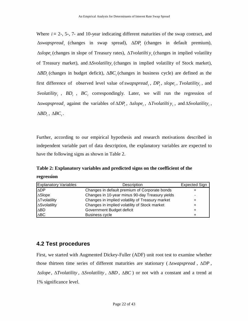
Where i = 2-, 5-, 7- and 10-year indicating different maturities of the swap contract, and

tswapspread (changes in swap spread), tDP (changes in default premium),

tslope (changes in slope of Treasury rates), tyTvolatilti (changes in implied volatility

of Treasury market), and tySvolatilit (changes in implied volatility of Stock market),

tBD (changes in budget deficit), tBC (changes in business cycle) are defined as the

first difference of observed level value of tswapspread , tDP , tslope , tyTvolatilit , and

tySvolatilit , tBD , tBC correspondingly. Later, we will run the regression of

tswapspread against the variables of tDP , tslope , tyTvolatilti , and tySvolatilit ,

tBD , tBC .

Further, according to our empirical hypothesis and research motivations described in

independent variable part of data description, the explanatory variables are expected to

have the following signs as shown in Table 2.

Table 2: Explanatory variables and predicted signs on the coefficient of the

regression

Explanatory Variables Description Expected Sign∆DP Changes in default premium of Corporate bonds +∆Slope Changes in 10-year minus 90-day Treasury yields -∆Tvolatility Changes in implied volatility of Treasury market +∆Svolatility Changes in implied volatility of Stock market +∆BD Government Budget deficit +∆BC Business cycle +

4.2 Test procedures

First, we started with Augmented Dickey-Fuller (ADF) unit root test to examine whether

those thirteen time series of different maturities are stationary ( swapspread , DP ,

slope , yTvolatilit , ySvolatilit , BD , BC ) or not with a constant and a trend at

1% significance level.


of 43

Second, to continue the empirical testing, we perform GARCH test to investigate the

impact of the changes in default risk premium slope, implied Treasury market volatility

and implied Stock market volatility on the interest rate swap spread with the exclusion of

the budget deficit and business cycle.

Third, to examine further, we apply the cointegration test to all the variables in pairs in

order to measure the extent of correlation between them.

Finally, based on the obtained test results, we conduct the extension of a multivariate

GARCH model by combining two Error Correction Terms into the regression. We will

discuss the test models and test results in detail in the following sections.

4.3 GARCH model

To test and quantify the effect of determinant factors on interest rate swap spread, we use

a Generalized Autoregressive Conditionally Heteroscedastic (GARCH) model developed

in a univariate form by Bollersle (1986) which expresses the conditional variance

changes over time as a function of past values of the squared errors and past conditional

variances, leaving the unconditional variance constant. The basic specification of

GARCH model is given by:

,12

112

12

ttt

The error term t denotes the real-valued discrete time stochastic process and 1t

is the information set available at time 1t .

1tt ~ ),0( 2tN

Where,

0 ,

01 ,

01 ,

111 , is sufficient for wide sense of stationary


of 43

ttt

t ~ IID and ),0( 2tN

This is a GARCH (1, 1) model, in which t2 is known as the conditional variance since

it is a one-period ahead estimate for the variance calculated on the basis of any past

information considered relevant. It is possible to interpret the current fitted variance, t2 ,

as a weighted function of a long-term average value dependent on , information about

volatility during the previous period ( 12

1 t ) and fitted variance from the model during

the previous period ( 12

1 t ). Additionally, it is found that a GARCH (1, 1) specification

is sufficient to capture the volatility dynamics in the data. Therefore, only one lagged

squared error and one lagged variance is needed.

GARCH model has several advantages over the pure ARCH model. First of all, the

GARCH model is more parsimonious, and avoids over-fitting. As a result, the model is

less likely to breach non-negativity constraints (Brooks, 2002). Secondly, a relatively

long lag in the conditional variance equation is often required. To avoid problems with

negative variance parameter estimates a fixed lag structure is called for in application of

the ARCH model (Bollerslev, 1986). In this light, the GARCH specification allows for

both a longer memory and a more flexible lag structure. Thirdly, as pointed out by

Bollerslev, the conditional variance is specified as a linear function of past sample

variances only in the ARCH (q) model, whereas the GARCH (p, q) model allows lagged

conditional variances to enter as well, this process corresponding to some kind of

adaptive learning mechanism. Fourthly, the virtue of the GARCH model enables a small

number of terms appear to perform as well as or better than an ARCH model with many.

Accordingly, in order to examine the effect of determinants of interest rate swap spread

jointly and provide further insight of variation of interest rate swap spread, the above

regression equation has been extended to a multivariate GARCH model of variables.

ptpqtqttttt 221

22121

211

21

2 2

p

j

jtjit

q

iit u

1

22

1


of 43

Where,

0q , 0p

0 , 0i , ,,,1 qi

0j , .,1 pi

4.4 Cointegration model

According to the economic theory, we think the two variables: budget deficit and

business cycle, might be cointegrated to some extent. A nonstationary variable tends to

wander extensively but some pairs of nonstationary variables can be expected to wander

in a way that they don�t drift apart from each other (Kennedy, 2001). Under such

consideration, we conduct the cointegation test between budget deficit and business cycle

since the data are I(1) which means that ECM (Error Correction Model) estimating

equation could be producing spurious results, such variables are said to be cointegrated.

We want to purge and estimate the nonstationary variables by differencing and using only

differenced variables if the data are shown to be nonstationary. We are quite interested in

the cointegration between budget deficit and business cycle since the cointegrating

combination is interpreted as an equilibrium relationship in which variables in the error-

correction term in an ECM can be shown. By testing the cointegration of the above two

variables, we could eliminate the unit roots. If the set of I(1) variables is cointegrated,

then regressing one on the others should produce residuals I(0).

4.5 GARCH with Error Correction Terms Model (ECT)

A full Error Correction Model (ECM) is performed to analyze the short-run dynamic

relationship between two variables. This Error Correction formulation in the regression is

ttt

tttttBCtBDt

DPTvol

SvolSLBCBDSS

87

65431,21,1

Error Correction Model is explained as follows:


of 43

First, we regress the swap spread on business cycle in the different maturity by using the

Least Squares method.

tBCtt BCSS ,

The residuals

tttBC BCSS ,

will be used for error correction in the final regression.

Second, we regress the swap spread on budget deficit using the Least Squares method.

tBDtt BDSS ,

The residuals

tttBD BDSS ,

are also used for error correction.

Finally we insert the residuals into the model.

ttt

tttttBCtBDt

DPTvol

SvolSLBCBDSS

87

65431,21,1

The coefficients are calculated by using GARCH specification.


of 43

5. Empirical findings This section contains our research analysis and the empirical testing results which include

ADF Unit root test results, GARCH model test results, Cointegration test results,

GARCH with Error Correction Terms and Hypothesis test results.

5.1 ADF Unit root test results

To proceed our tests, we started with Augmented Dickey-Fuller (ADF) unit root test to

examine whether these thirteen time series of different maturities are stationary

( swapspread , DP , slope , yTvolatilit , ySvolatilit , BD , BC ) or not with a

constant and a trend at 1% significance level. The test result shows in the Table 3.

Table 3: Augmented Dickey-Fuller unit root test (first difference of the level data)

1st Difference 1st DifferenceVaribles Constant only Constant and linear trend

∆Swap spread 2Y -11,792 -11,743∆Swap spread 5Y -11,303 -11,280∆Swap spread 7Y -12,094 -12,051∆Swap spread 10Y -11,259 -11,222

∆DP 2Y -13,331 -13,267∆DP 5Y -13,291 -13,259∆DP 7Y -12,253 -12,244∆DP 10Y -11,089 -11,826∆Slope -9,133 -9,334

∆Tvolatility -7,473 -7,387∆Svolatility -8,987 8,944

∆Budget deficit -3,198 -3,547∆Business cycle -8,731 -8,684

Note: both resulting test values of 1st difference & constant only and 1st difference & constant and linear trend are far more negative than the critical value at 1% significance level (-3.497). Therefore we concluded that 13 time series do not have unit root. In other words, they are stationary time series data.


of 43

5.2 GARCH analysis

In order to investigate the variation of swap spread, we test the volatility of swap spread

based on the specification of GARCH model in the form of the following regression

equation, in which we regress the changes in swap spread against changes in default

premium, slope of yield curves, implied Treasury market volatility and implied Stock

market volatility with the exclusion of budget deficit and business cycle6. The data used

in this GARCH estimation is the first difference of the observed level data. The test

results are presented in Table 4.

tititi BCBD ,6,5,

Table 4: GARCH Test Results

Coefficient Z-stat P-value Coefficient Z-stat P-value Coefficient Z-stat P-value Coefficient Z-stat P-valueb 1 0,005 -0,104 0,917 0,031 0,361 0,718 0,049 0,659 0,510 0,053 0,579 0,562

(0.046) (0.086) (0.074) (0.091)b 2 0,045 1,453 0,146 0,009 0,311 0,756 0,016 0,577 0,564 0,028 0,914 0,361

(0.031) (0.028) (0.028) (0.031)b 3 5,176 0,794 0,427 6,101 0,708 0,479 -2,237 -0,201 0,841 2,550 0,187 0,852

(6.522) (8.619) (11.117) (13.622)b 4 3,488 1,557 0,120 1,131 0,434 0,665 3,267 1,072 0,284 1,161 0,328 0,743

(2.241) (2.608) (3.049) (3.540)R2

0,048 0,033 0,034 0,014

2-year 5-year 7-year 10-year

Note: all the figures in ( ) are the standard errors.

It can be seen from Table 4, that the coefficients on four independent variables in the

conditional variance equation are not all statistically significant. In particular, the proxy

variables of implied volatility of Treasury market and implied volatility of Stock market

which have 5.17 and 3.48 for 2-year maturity and 2.55 and 1.16 for 10-year maturity,

respectively. Furthermore, the P-values of four maturities are overall not statistically

significant even at a 10% significance level. In other words, the null hypothesis of our

empirical research can not be rejected as statistically significant.

6 The reason of excluding these two variables here is that we suspect that these two variables are cointegrated, therefore, we conduct the cointegration test after we obtaining the results from the simple GARCH test.

titititiiti ySvolatilityTvolatilitslopeDPswapspread 4,3,2,1,0,,


of 43

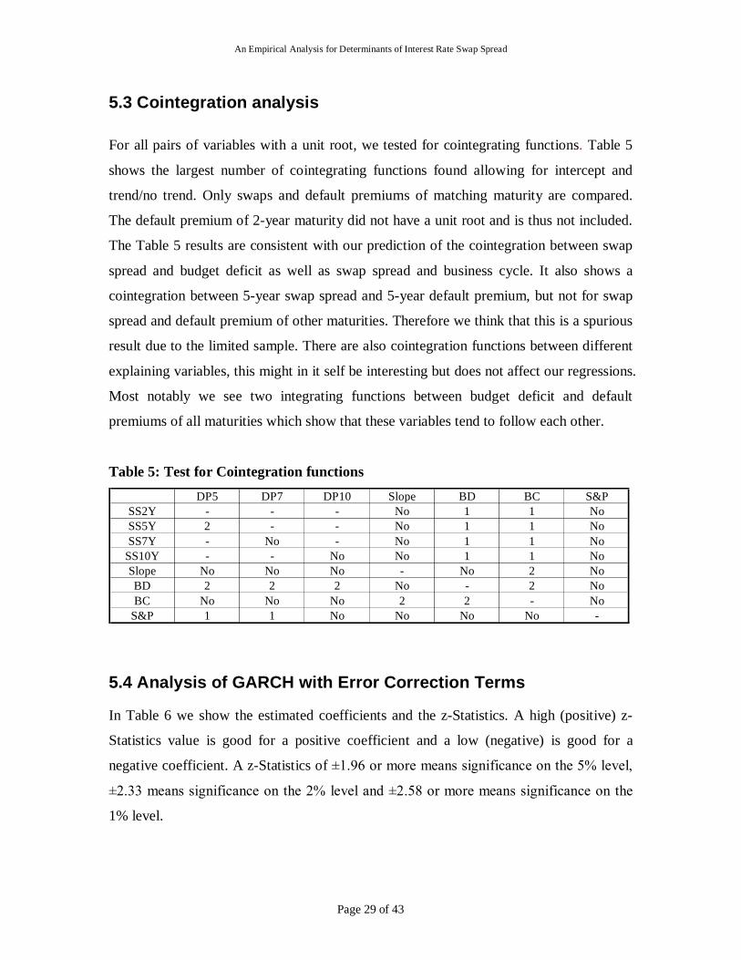
5.3 Cointegration analysis

For all pairs of variables with a unit root, we tested for cointegrating functions. Table 5

shows the largest number of cointegrating functions found allowing for intercept and

trend/no trend. Only swaps and default premiums of matching maturity are compared.

The default premium of 2-year maturity did not have a unit root and is thus not included.

The Table 5 results are consistent with our prediction of the cointegration between swap

spread and budget deficit as well as swap spread and business cycle. It also shows a

cointegration between 5-year swap spread and 5-year default premium, but not for swap

spread and default premium of other maturities. Therefore we think that this is a spurious

result due to the limited sample. There are also cointegration functions between different

explaining variables, this might in it self be interesting but does not affect our regressions.

Most notably we see two integrating functions between budget deficit and default

premiums of all maturities which show that these variables tend to follow each other.

Table 5: Test for Cointegration functions

DP5 DP7 DP10 Slope BD BC S&PSS2Y - - - No 1 1 NoSS5Y 2 - - No 1 1 NoSS7Y - No - No 1 1 No

SS10Y - - No No 1 1 NoSlope No No No - No 2 NoBD 2 2 2 No - 2 NoBC No No No 2 2 - No

S&P 1 1 No No No No -

5.4 Analysis of GARCH with Error Correction Terms

In Table 6 we show the estimated coefficients and the z-Statistics. A high (positive) z-

Statistics value is good for a positive coefficient and a low (negative) is good for a

negative coefficient. A z-Statistics of ±1.96 or more means significance on the 5% level,

±2.33 means significance on the 2% level and ±2.58 or more means significance on the

1% level.


of 43

The significant results we find are: Business cycle of 5-year and 7-year maturity have

significance on the 5% and 2% level respectively (negative correlation). The slope has

significance on the 1 % level for all maturities (positive correlation). The stock market

volatility has significance on the 5% level for the 7-year maturity (positive correlation).

The default premium has significance at the 1% level for 2-year and -year maturity and at

the 2% level for 5-year maturity and at the 5% level for the 10-year maturity (negative

correlation).

Table 6: Coefficients, z-Statistics and R2 for ECM

Coeff z-Stat Coeff z-Stat Coeff z-Stat Coeff z-Statb 1 -0,110 -0,700 0,000 0,409 0,000 0,496 -0,141 -1,278b 2 0,037 0,252 -0,116 -1,088 -0,147 -1,517 0,000 -0,319b 3 0,000 0,214 0,000 0,135 0,000 0,060 0,000 -1,383b 4 -0,080 -0,710 -0,364 -2,285 -0,343 -2,414 -0,274 -1,529b 5 0,041 2,775 0,063 3,261 0,064 3,585 0,069 3,454b 6 1,862 1,716 1,362 1,000 3,015 1,971 -0,352 -0,245b 7 -1,035 -0,229 0,802 0,106 -10,031 -1,436 -5,263 -0,607b 8 -0,202 -3,226 -0,209 -2,338 -0,162 -2,901 -0,607 -2,008

R 2 0,210 0,090 0,089 0,133

2YR 5YR 7YR 10YR

5.5 Hypothesis Test Results

Here is our hypothesis analysis based on our regression results.

(1) Changes in the IR swap spread will be related positively to changes in the default

premium in corporate bond market.

It is in the default premium that we find the strongest correlation with swap spread. ECM

shows a strong correlation with z-statistics of �2.01 or better, indicating significance at

the 5% level for 10-year maturity, and z-statistics of �3.2 3 for 2-year maturity indicating

significance at the 1% level. However, this correlation is negative, disproving our

hypothesis. The negative correlation can be quite easily seen in the above graph. The

relation between swap spread does not fit with the intuitive assumption that uncertainty in

the market will lead to larger swap spread and default premium. Clearly the relation has a

more complicated explanation and further investigation is needed; this is however not

within the scope of this thesis.


of 43

Figure 5: The movement of swap spread and default premium of 2-year maturity

-0.5

-0.4

-0.3

-0.2

-0.1

0

0.1

0.2

0.3

Jun-98

Dec-98

Jun-99

Dec-99

Jun-00

Dec-00

Jun-01

Dec-01

Jun-02

Dec-02

Jun-03

Dec-03

Jun-04

Dec-04

Jun-05

Dec-05

Jun-06

Dec-06

∆Sw ap spread 2Y(fd) ∆DPt(fd) 2Y

(2) Changes in the IR swap spread will be related negatively to changes in the slope

of yield curve of Treasury Securities.

The ECM shows significance in the slope of yield curve only for 5 and 7-year maturity

(z-Stat. of -2.28 and �2.41, respectively). This is significant at the 2% level. Therefore,

our results strongly suggest that changes in the interest rate swap spread and the changes

in the slope of yield curve of Treasury Securities. The observed correlation is negative

which supports our hypothesis, which states that if future short term interest will be

higher (positive slope), then there is less uncertainty in the market because of expected

good times and less uncertainty leads to smaller swap spread.


of 43

Figure 6: The movement of swap spread of 2-year maturity and slope of Treasury

yields

-0.8

-0.6

-0.4

-0.2

0

0.2

0.4

0.6

0.8

1

1.2

Jun-98

Dec-98

Jun-99

Dec-99

Jun-00

Dec-00

Jun-01

Dec-01

Jun-02

Dec-02

Jun-03

Dec-03

Jun-04

Dec-04

Jun-05

Dec-05

Jun-06

Dec-06

∆Slope(t)fd ∆Sw ap spread 2Y(fd)


implied Treasury market volatility.

The Treasury market volatility shows no significant correlation with the swap (z-Stat. of -

0.22895 and -0.60729 in 2 year and 10 year). We can neither prove nor disprove our

hypothesis from this data. However, it seams that any correlation would be quite weak. In

the future, when more statistics are available, it might be possible to observe a

correlation. It is, however, not possible now, due to the limited time that the swap spread

market has existed.


implied Stock market volatility.

The stock market volatility shows a positive correlation with share spread with

significance on the 5% level for the 7-year maturity. This supports our hypothesis,

although only for the 7-year maturity. The reasoning behind our hypothesis is that both

share spread and stock market volatility are signs of insecurity in the market and should

thus be positively correlated.


of 43


government budget deficit index.

We see no significance for a correlation with government budget deficit (Z-Stat. of

0.21380and -1.38262 in 2 year and 10 year). Again, there is no significant correlation to

prove or disprove the hypothesis. The statistics available are quite limited as the swap

market has existed for only a short time. Any correlation would have to be quite strong to

be visible.


business cycle.

The ECM shows a negative correlation for 5-year and 7-year maturity (z-Stat. of -2.28

and -2.41 respectively, significant at the 2% level). Even though it shows the strong

correlation between these two variables, it disproves our hypothesis at the 2% level.

Regression including Business cycle is complicated by the fact that date for Business

cycle only exists on a quarterly basis and two out of three data points have to be

interpolated in this regression. However, we did try interpolation in two ways; the one

used in the presented regressions is simply that we assume the variable to be constant for

the three months in a quarter. At the same time we tried with linear interpolation where

we assumed the value of the quarter to apply for the middle month of the quarter and vary

linearly until the middle month of the next quarter, i.e. if n is the middle month of quarter

1 and n+3 is the middle month of quarter 2, the values of the months in between are

BCn+1=0.667*BCn+0.333*BCn+3 and BCn+2=0.333*BCn+0.667*BCn+3. The results of the

regressions with the two different interpolations schemes did not differ much and we

chose to use the simpler one.


of 43

Figure 7: The movement of swap spread of 2-year maturity and business cycle

-0.5

-0.4

-0.3

-0.2

-0.1

0

0.1

0.2

0.3

Jun-98

Dec-98

Jun-99

Dec-99

Jun-00

Dec-00

Jun-01

Dec-01

Jun-02

Dec-02

Jun-03

Dec-03

Jun-04

Dec-04

Jun-05

Dec-05

Jun-06

Dec-06

∆Sw ap spread 2Y(fd) Business Cycle


of 43

6. Conclusions This part concludes what our empirical research is about, the data, the methodology we

use and the results we obtained from the tests. Moreover, we point out what is missing in

this study and present the research suggestions for future work.

Our paper uses a multivariate GARCH model with Error Corrections Terms (ECM) to

investigate the determinants of swap spreads in the U.S. interest rate market. We have

used monthly data of 2-, 5-, 7-, 10-year maturity from June 30, 1998 to March 31, 2007

for a total of 106 observations to empirically investigate the importance of the

determinants of interest rate swap spread in U.S derivative market. According to our

research results, we found that the movement of interest rate swap spread is negatively

related to changes in the slope of yield curve of Treasury Securities which consistent with

our hypothesis. We also found out that changes in the IR swap spread will be related

positively to changes in the implied Stock market volatility; but we disprove our

hypothesis that the changes in the swap spread will be related positively to changes in the

default premium in corporate bond market. We found, however, that swap spreads in the

U.S. market show negatively strong correlation with default premium with z-statistics of

�2.01 or better. We also conclude that changes in the interest rate swap spread will be

related negatively to changes in the business cycle. We think, however, that the business

cycle is very complicated due to the nature of data. There is some evidence by

Litzenberger (1992) that the allocation of risk between swap counter parties varies over

business cycles.

We have to admit that there are some important factors which have not been built into our

model. For example, we noticed swap spreads have a peak in the end of 1990s and early

2000. It might imply that swap spread is subject to some sort of shocks. We have not

considered running regressions of determinants of swap spreads jointly for swap spreads

of different terms to maturity. Based on the economy theory and empirical research

results, it is shown that the interest rate swap market is not segmented to between

different maturities (In, Brown and Fang, 2003). Further, there are some evidences that


of 43

the U.S. market also responds to conditions in the UK and Australia market due to the

international links between financial markets. We leave these issues for future research.


of 43

7. Acknowledgements

We would like to thank Professor Hossein Asgharian for useful comments and research

support, and also thanks to Doris, Jens, Torbjorn for helpful support and suggestions.

Thanks to our parents for infinite support and love.


of 43

8. Appendix Figure 1: The movement of swap rate and the slope of the yield curve

0

1

2

3

4

5

6

7

8

9

Jun-98

Dec-98

Jun-99

Dec-99

Jun-00

Dec-00

Jun-01

Dec-01

Jun-02

Dec-02

Jun-03

Dec-03

Jun-04

Dec-04

Jun-05

Dec-05

Jun-06

Dec-06

USSWAP10 Curncy 10YSR Slope(t)

Figure 2: The movements of swap rates and the slope of the yield curve

0

1

2

3

4

5

6

7

8

9

Jun-98

Dec-98

Jun-99

Dec-99

Jun-00

Dec-00

Jun-01

Dec-01

Jun-02

Dec-02

Jun-03

Dec-03

Jun-04

Dec-04

Jun-05

Dec-05

Jun-06

Dec-06

USSWAP2 Curncy 2YSR USSWAP5 Curncy 5YSR USSWAP7 Curncy 7YSR

USSWAP10 Curncy 10YSR Slope(t)


of 43

Figure 3: The movement of swap spread and default premium

0.0

0.2

0.4

0.6

0.8

1.0

1.2

1.4

1.6

Jun-98

Dec-98

Jun-99

Dec-99

Jun-00

Dec-00

Jun-01

Dec-01

Jun-02

Dec-02

Jun-03

Dec-03

Jun-04

Dec-04

Jun-05

Dec-05

Jun-06

Dec-06

Sw ap spread 10Y(t) DPt 10Y

Figure 4: Output of univariate regression of swap spread, business cycle and residual business cycle of 5-year maturity

-0.2

0.0

0.2

0.4

0.6

0.8

1.0

1.2

Jun-98

Dec-98

Jun-99

Dec-99

Jun-00

Dec-00

Jun-01

Dec-01

Jun-02

Dec-02

Jun-03

Dec-03

Jun-04

Dec-04

Jun-05

Dec-05

Jun-06

Dec-06

Sw ap spread 5Y(t) Business Cycle Residual Bus5yr


of 43

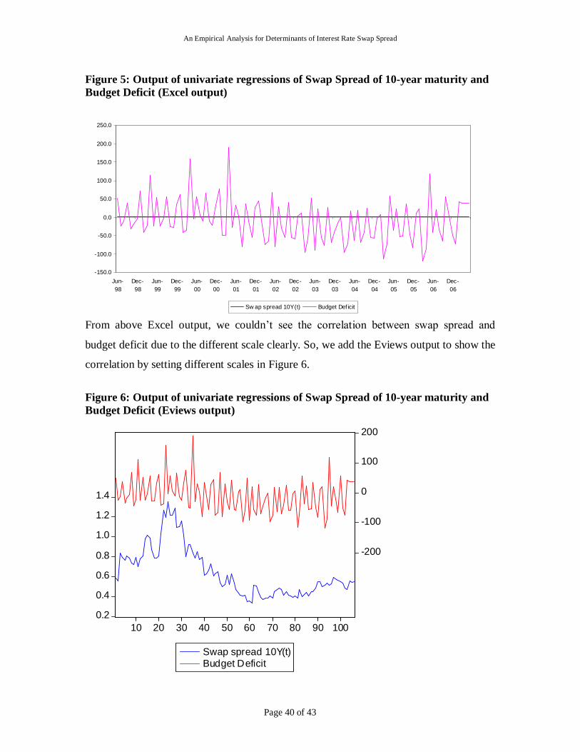
Figure 5: Output of univariate regressions of Swap Spread of 10-year maturity and Budget Deficit (Excel output)

-150.0

-100.0

-50.0

0.0

50.0

100.0

150.0

200.0

250.0

Jun-98

Dec-98

Jun-99

Dec-99

Jun-00

Dec-00

Jun-01

Dec-01

Jun-02

Dec-02

Jun-03

Dec-03

Jun-04

Dec-04

Jun-05

Dec-05

Jun-06

Dec-06

Sw ap spread 10Y(t) Budget Def icit

From above Excel output, we couldn�t see the correlation between swap spread and

budget deficit due to the different scale clearly. So, we add the Eviews output to show the

correlation by setting different scales in Figure 6.

Figure 6: Output of univariate regressions of Swap Spread of 10-year maturity and Budget Deficit (Eviews output)

0.2

0.4

0.6

0.8

1.0

1.2

1.4

-200

-100

0

100

200

10 20 30 40 50 60 70 80 90 100

Swap spread 10Y(t)Budget Deficit


of 43

9. References

Bernadette A. Minton (1996) An empirical examination of basic valuation models for

plain vanilla U.S interest rate swaps.

Bondnar,G.M., Hayt,G.S., Marston, R.C., & Smithson,C.W. (1995). Wharton survey of

derivatives usage by US non-financial firms. Financial Manangement, 24, 104-114.

Brooks, C (2002) Introductory Econometrics for Finance.

Brown, K. C., Harlow, W. V., and Smith, D.J. (1994). A Empirical Analysis of Interest

Rate Swap Spreads. Jounal Of Fixed Income, 3, 61-78.

Collin-Dufresne, P., and Solnik, B. (2001). On the Term Structure of Default Premia in

the Swap and LIBOR Markets. Journal of Finance, 56, 1095-1115.

Cooper, I., Melo, A S., 1991. The Default Risk of Swaps. Journal of Finance 48, 597-620.

Darrell Duffie; Kenneth J. Singleton, An Econometric Model of the Term Structure of

Interest-Rate Swap Yields, The Journal of Finance, Vol. 52, No. 4. (Sep., 1997), pp.

1287-1321.

Dai, Q., Singletion, K.J., 1997 Specification analysis of Affine term structure models,

Working Paper: Stanford University.

Enrico Bernini, Counterparty Credit Risk and the Determinants of U.S. Interest Rate

Swaps. 2005, Banca Itesa, NYU and Bocconi University.

Eric H. Sorensen and Thierry F. Bollier, Pricing swap default risk. Financial Analysts

Journal: May/Jun 1994; 50,3; ABI/ INFORM Global.


of 43

Francis Ina, Rod Brown B, Victor Fang, Modeling volatility and changes in the swap

spread. International Review of Financial Analysis 12 (2003) 545-561.

Frank Fehle , The components of interest rate swap spreads. The Journal of Futures

Markets, Vol. 23, No. 4, 347-387 (2003).

Hua He (2000) Modeling term structure of swap spreads, Yale School of Management

June 2000, working paper No.00-16.

Hull, J (2005) Options, Futures and Other Derivates, 149-150.

Hull, J., 1989. Assessin Credit Risk in Financial Institution�s Off-Blance Sheet

Commitments. Journal of Financial and Quantitative Analysis 24, 489-501.

In, F., Brown, R., Fang, V. (2003) Modeling volatility and changes in the swap spread.

International Review of Financial Analysis, (12) 545-561.

Jun Liu, Francis A. Longstaff, Ravit E. Mandell (2006) The Market Price of Risk Interest

Rate Swaps: the Roles of Default and Liquidity Risks. Journal of Business, 2006. vol.79.

no. 5.

John Kambhu, Federal Reserve Bank of New York, Staff Reports, Trading Risk and

Volatility in Interest Rate Swap Spreads, Staff Report no. 178, February 2004.

Jame Bicksler; Andrew H. Chen, Analysis of interest rate swaps, The Journal of Finance,

Vol. 41, No. 3, Papers and Proceedings of the Forty-Fourth Annual.

Kodjo M. Apedjinou, What drives interest rate swap spreads? 2003 An empirical analysis

of structural changes and implications for modeling t of the swap term structure.

Kennedy, P. (2002) A Guide to Econometrics.


of 43

Mark Grinblatt, An Analytic Solution for Interest Rate Swap Spreads. Anderson School

of Management, 1995, paper 9�94.

Lang, L., Litzenberger, R and Liu (1998) Determinants of interest rate swap spread,

Journal of Banking & Finance 22, 1507-1532.

Lekkos I, Milas C, (2001) Identifying the factors that affect interest rate swap spread:

some evidence from the U.S and the U.K.

Litzenberger, R.H. (1992). Swaps: Plain and fanciful. Journal of Finance, 47,597-620.

René M. Stulz, Rethinking Risk Management, the Ohio State University Journal of

Applied Corporate Finance.

Sorensen, E.H., Bollier, T.F., (1994) Pricing Swap Default Risk. Financial Analysis

Journal 50, 23-33.

Timan, S. 1992. Interest Rate Swaps and Corporate Finance Choices. Journal of Finance

47, 1503-1516.

Turnbull, S.M. (1987). Swaps: A zero sum game? Financial Management, 16, 15-21.

Victor Fang, Ronny Muljono, An empirical analysis of the Australian dollar swap spreads,

Received 13 August 2001; accepted 5 June 2002.

An Empirical Analysis for Determinants of Interest Rate ...

Documents

Transcript of An Empirical Analysis for Determinants of Interest Rate ...