An elastic demand schedule-based multimodal assignment ... · An elastic demand schedule-based...
25
RESEARCH PAPER An elastic demand schedule-based multimodal assignment model for the simulation of high speed rail (HSR) systems Ennio Cascetta • Pierluigi Coppola Received: 28 October 2011 / Accepted: 19 February 2012 / Published online: 4 April 2012 Ó Springer-Verlag + EURO - The Association of European Operational Research Societies 2012 Abstract High speed rail (HSR) represents the future of medium-haul intercity transport. In fact, a number of HSR projects are being developed all over the world despite the financial and economic crisis. Such large investments require reliable demand forecasting models to develop solid business plans aiming at optimizing the fares structures and the timetables (operational level) and, on the other hand, at exploring opportunities for new businesses in the long period (strategic level). In this paper, we present a models system developed to forecast the national passenger demand for different macroeconomic, transport supply, and HSR market scenarios. The core of the model is based on the simulation of the competition between transportation modes (i.e. air, auto, rail), railways services (intercity vs. high speed rail) and HSR operators, using an explicit representation of the timetables of all competing modes/services/runs (schedule-based assignment). This requires, in turn, a diachronic network representation of the transport supply for scheduled services and a nested logit model of mode, service, operator, and run choice. To authors’ knowledge this represents the first case of elastic demand, schedule-based assign- ment model at national scale to forecast HSR demand. The overall modeling framework has been calibrated based on extensive traffic counts and mixed RP–SP interviews gathered between 2009 and 2011, on the Italian multimodal transporta- tion system. The results of the models estimation are presented, and, some appli- cations to test HSR service options (i.e. fares and timetable) of a new operator entering the HSR market and competing with the national incumbent are discussed. E. Cascetta Dipartimento di Ingegneria dei Trasporti, Universita ` di Napoli ‘‘Federico II’’, Via Claudio 21, 80125 Naples, Italy e-mail: [email protected] P. Coppola (&) Dipartimento di Ingegneria dell’Impresa, Universita ` di Roma ‘‘Tor Vergata’’, Via del Politecnico 1, 00133 Rome, Italy e-mail: [email protected] 123 EURO J Transp Logist (2012) 1:3–27 DOI 10.1007/s13676-012-0002-0
Transcript of An elastic demand schedule-based multimodal assignment ... · An elastic demand schedule-based...
RESEARCH PAPER
An elastic demand schedule-based multimodalassignment model for the simulation of highspeed rail (HSR) systems
Ennio Cascetta • Pierluigi Coppola
Received: 28 October 2011 / Accepted: 19 February 2012 / Published online: 4 April 2012
� Springer-Verlag + EURO - The Association of European Operational Research Societies 2012
Abstract High speed rail (HSR) represents the future of medium-haul intercity
transport. In fact, a number of HSR projects are being developed all over the world
despite the financial and economic crisis. Such large investments require reliable
demand forecasting models to develop solid business plans aiming at optimizing the
fares structures and the timetables (operational level) and, on the other hand, at
exploring opportunities for new businesses in the long period (strategic level). In
this paper, we present a models system developed to forecast the national passenger
demand for different macroeconomic, transport supply, and HSR market scenarios.
The core of the model is based on the simulation of the competition between
transportation modes (i.e. air, auto, rail), railways services (intercity vs. high speed
rail) and HSR operators, using an explicit representation of the timetables of all
competing modes/services/runs (schedule-based assignment). This requires, in turn,
a diachronic network representation of the transport supply for scheduled services
and a nested logit model of mode, service, operator, and run choice. To authors’
knowledge this represents the first case of elastic demand, schedule-based assign-
ment model at national scale to forecast HSR demand. The overall modeling
framework has been calibrated based on extensive traffic counts and mixed RP–SP
interviews gathered between 2009 and 2011, on the Italian multimodal transporta-
tion system. The results of the models estimation are presented, and, some appli-
cations to test HSR service options (i.e. fares and timetable) of a new operator
entering the HSR market and competing with the national incumbent are discussed.
E. Cascetta
Dipartimento di Ingegneria dei Trasporti, Universita di Napoli ‘‘Federico II’’,
Via Claudio 21, 80125 Naples, Italy
e-mail: [email protected]
P. Coppola (&)
Dipartimento di Ingegneria dell’Impresa, Universita di Roma ‘‘Tor Vergata’’,
Via del Politecnico 1, 00133 Rome, Italy
e-mail: [email protected]
123
EURO J Transp Logist (2012) 1:3–27
DOI 10.1007/s13676-012-0002-0

Keywords National travel demand � Mode/service/run choice modeling � Mixed
RP–SP surveys � HSR operators’ competition
Introduction
High speed rail (HSR) represents the future of medium-haul intercity transport. In
fact, a number of HSR projects are being developed all over the world despite the
current financial and economic crisis (Ivan 2011). Such large investments require
reliable demand forecasting to develop solid business plans aiming, on the one hand,
at optimizing the medium-term profits leveraging on the fares structures and the
timetables (operational level) and, on the other hand, at exploring the opportunities
for new businesses such as new routes, innovative on-board travel amenities (e.g.
internet availability, movies projections) which in turn would require duly designed
rolling stock, new customized services and other strategic choices, coping with the
socio-economic changes that could be induced by HSR.
Basically, HSR demand forecasting requires the evaluation of three demand
components (Table 1): the diverted demand, which derives from the travelers’
mode choice diversion toward HSR either from other modes (e.g. auto, air) or
other rail services (e.g. intercity); the economy-based demand growth, which is
linked to the trends of the National and International economic systems, under the
assumption that the more the people are wealthy the more they travel; and the
induced demand which depends either ‘‘directly’’ on the generalized travel cost,
i.e. changes in travel choices such as trip frequency, destination or activity pattern,
e.g. the trip becomes more frequent because traveling with HSR is faster, cheaper
and/or more comfortable, or ‘‘indirectly’’ due to modifications of the travelers’
mobility or lifestyle choices, e.g. travelers start commuting (i.e. making more
frequent trips) due to the relocation of the residence or of the workplace, and partly
due to changes in land use, e.g. new residents, jobs and activities interconnected
thanks to HSR.
Table 1 Taxonomy of the impacts on HSR demand
Endogenous factors Exogenous factors
Diverted demand
From other modes e.g. Shift from air/auto to HSR
From other rail services e.g. Shift from Intercity to HSR
Induced demand
Direct e.g. Changes of trip frequency,
destination or related activity
pattern
Indirect e.g. Increase of mobility due to
change in life-styles and land use
(Economy-based)
demand growth
e.g. Increase of the overall mobility
due to economic growth
4 E. Cascetta, P. Coppola
123

To forecast the impacts of the new HSR services, a general modeling architecture
has been developed (Ben-Akiva et al. 2010; Cascetta and Coppola 2011) consisting
of the following integrated models:
• the ‘‘National demand growth’’ model, which projects the base year total OD
volumes to future years, according to assumed macroeconomics trends;
• the ‘‘mode/service/run choice’’ model, which estimates the market share of
different inter-urban transportation modes, including alternative rail services,
such as intercity, high-speed, 1st and 2nd class and different HSR operators (i.e.
competition within HSR mode) characterized by different fares, different
timetables, different on-board services and other ‘‘brand-related’’ characteristics;
• the ‘‘induced demand’’ model which estimates the additional HSR demand due
to the improvement of HSR level of services (i.e. new services, travel time
reductions, etc.);
• the stochastic assignment model which loads the multimodal and multiservice
(diachronic) network to estimate the flows on the individual trains and flights.
Such models system has been calibrated over the Italian national case study,
which represents an interesting field of application. In fact, the HSR in Italy is still
under development meaning that the travel times station-to-station, which have
already been reduced by about 30–40 %, are expected to be further reduced with the
completion of the new underground bypass-stations in Bologna and Firenze that will
allow the speeding up of the service in such dense urban areas. In this respect, it
represents an ideal test site to validate the model forecasting in the near future by a
before-and-after analysis. Moreover, starting from 2012, the new HSR operator
‘‘Nuovo Trasporto Viaggiatori’’ (NTV) will be operative on the national HSR
network, competing with the incumbent Trenitalia, giving rise to the first case in the
World of competition among HSR operators on the same line (i.e. multiple
operators on a single infrastructure).
In this paper, we will focus on the sub-models developed to estimate individuals
trains’ passengers flows as the result of the diverted demand both from other modes
and from other rail services, i.e. the multimodal, elastic-demand, stochastic network
loading assignment model. To this aim, the schedule-based approach is followed.
With respect to the traditional frequency-based approach typically adopted for the
simulation of transport services both at the urban and intercity level, the schedule-
based approach allows considerations of time-dependent characteristics of the
supply and of the demand, and simulates the travelers’ choices between
transportation modes (e.g. air, auto, rail) and rail services (e.g. intercity, HSR),
but also between different individual runs (i.e. trains or flights) characterized by
different fares, different on-board-services, and arrival/departure times. The strength
of the such approach, compared to the others proposed in literature for HSR demand
forecasting, stems from the fact that it allows also testing operational policies such
as changes in the fare structure (e.g. based on differentiated time-of-day and train-
specific fares) and modification of the timetables, not necessarily related to the rail
market. In other words, the number of travelers on a given HSR train in a certain rail
segment will depend on the fares and timetables of competing railways, air and on
car opportunities. Moreover, as the arrival and departure times of single runs are
An elastic demand schedule-based multimodal assignment 5
123

explicitly represented in a schedule-based supply models, such approach allows
computing correctly the transfer times on those paths including modes/runs
interchanges. This greatly improves the generation of the available paths on the
multimodal and multiservice network (choice set generation), but also allows
computing more precisely the transfer time on each path connecting a given OD
pair, which is an attribute significantly affecting the mode choice.
The paper is organized as follows. In Sect. 2, the state of the art of national
demand models developed for forecasting HSR demand is presented and a models
classification is proposed. Section 3 describes the overall schedule-based assign-
ment model including: (a) the characteristics of the HSR services in the study area
and the supply models used for the computation of the level-of-service (l.o.s.)
attributes; (b) the mode-service-operator-run choice model including some speci-
fication of the utility function for different travel purposes; and (c) the assignment
procedure to load the OD demand flows on the networks and to forecast the traffic
flows on the single HSR trains connecting different OD pairs, characterized by
different fares, on-board services and timetables. In Sect. 4, some applications of the
overall modeling architecture to test the elasticity of the demand to the HSR fares
and to estimate the effects of different timetables to increase the patronage of the
new incoming HSR operator are discussed. Conclusions and further research areas
are finally reported in Sect. 5.
HSR demand forecasting: state of art
HSR demand forecasting models can be distinguished in aggregate and disaggregate
(Table 2).
Aggregate models forecast railways demand based on aggregate demand
elasticity values to GDP variations, car and railway travel times, fuel costs, car
ownership, population and so on. Such models make use of large data sets obtained
from recorded ticket sales and from travel surveys, as well as from national
statistics. They have successfully predicted the rail demand growth (see for instance
Wardman 2006), but their capabilities are limited when there are big technological
Table 2 Classification of disaggregate HSR demand forecasting models
Frequency-based Scheduled-based
Multi-modal
Multi (rail) service Ben-Akiva et al. (2010) Cascetta and Coppola (2011)
Single (rail) service Roman et al. (2007)
Yao and Morikawa (2005)
Froidh (2008)
Mono-modal
Multi (rail) service Couto and Graham (2008)
Hsu and Chung (1997)
Single (rail) service Urban case studies Urban case studies
6 E. Cascetta, P. Coppola
123

and economic changes. Moreover, aggregate demand forecasting models by
definition cannot simulate flows on individual rail segment or trains, estimates
needed to design and assess both infrastructures and services.
Disaggregate models can be mono-modal and multi-modal. Mono-modal models,
typically conceived to simulate demand in urban context, focus on a specific mode
and forecast the impact of a new technology or an operational improvement on the
demand and the overall performances on that modes; an example for HSR can be
found in Hsu and Chung (1997) or in Couto and Graham (2008). On the other hand,
most of the HSR demand forecasting models are disaggregate (mainly behavioral)
modeling structures simulating explicitly the competition between Rail and other
modes (multi-modal models) and/or between rail services, e.g. Intercity and HSR
(multi-service models). Such models have been applied to forecast HSR demand in
Germany (Mandel et al. 1997), Sweden (Froidh 2005, 2008), Spain (Roman et al.
2007; Martin and Nombela 2007), Japan (Yao and Morikawa 2005) and Korea (Park
and Ha 2006). Most of these models focus on the competition between air and HSR
(long distance passenger models), some of them deal also with auto competition and
very few include the competition between rail services and operators (see for
instance Ben-Akiva et al. 2010).
Concerning the modeling approach to the simulation, it is well-known that the
common practice in modeling scheduled transport systems, both at the urban and
intercity levels, involves the representation of services as lines, with the time
dimension taken into account through the average line frequency, through which the
average on-board loads and performances can be calculated (frequency-based
approach).
This approach is not satisfactory in many applications, typical of low-frequency
systems and/or operational planning (e.g. timetable design), in which we have to
take into account time-dependent characteristics of the service and of the demand
and we need to analyze the loads on each vehicle. In such cases, scheduled services
can be better represented by individual vehicle trips which define individual
connections within a given timetable (e.g. a given train connection) and the
modeling framework, in which all its components (demand, supply, path choice and
assignment) account explicitly for the timetable, is defined as the schedule-based
approach (Wilson and Nuzzolo 2004). All the models presented in the literature to
forecast HSR demand, follow a frequency-based approach. To authors’ knowledge
the model presented in this paper is the first example of an elastic demand,
multimodal, schedule-based assignment model developed at national scale.
The elastic demand schedule-based multi-modal assignment model
An elastic demand, multi-modal, schedule-based assignment models consists of (see
Fig. 1):
1. a supply model, representing explicitly the individual runs (e.g. trains,
flights,…) with given departure/arrival times at stops (e.g. a diachronic
network) in addition to a static road network;
An elastic demand schedule-based multimodal assignment 7
123

2. a time-dependent segmentation of origin–destination (OD) matrices, according
to the travelers’ desired departure time (DDT) and desired arrival time (DAT)
distributions;
3. a joint mode-service-operator-run choice model;
4. an assignment model loading the flow on the run-based (i.e. diachronic)
network.
The overall modeling framework is currently based on a zoning system
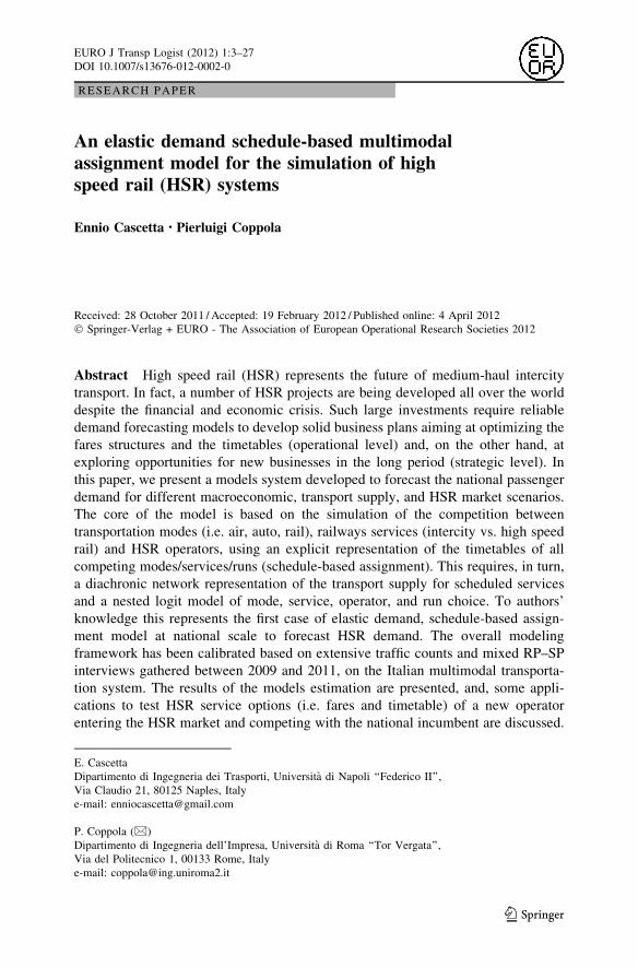
consisting of 220 zones (Fig. 2). The study area includes all the Italian regions
with the exception of the islands of Sicily and Sardinia. The regions of Abruzzo,
Molise (on the Adriatic corridor), Umbria (central Italy) and the regions of
Trentino-Alto Adige and Valle d’Aosta (in the North) are each represented by
one zone. All the other Italian provinces have been split into two zones: one
zone for the main city of the province and one zone for the rest of the province.
Moreover, the main Italian cities have been further divided into several zones:
Roma into 13 zones; Napoli into 8 zones; Torino into 6 and Milano into 10
zones.
Fig. 1 Schematic representation of the assignment procedure
8 E. Cascetta, P. Coppola
123
Supply model (diachronic network)
In terms of supply modeling, the schedule-based approach requires a run-based
supply representation in which individual vehicle trips with arrival/departure times
at stops are considered. In the literature, there are three main run-based
representations of transit services: the diachronic network (Nuzzolo and Russo
1993) also referred to as time-expanded network (Ahuja et al. 1993); the dual
network (Anez et al. 1996) and the mixed line-based/database supply model (Tong
and Richardson 1984; Wong and Tong 1999). In the proposed modeling framework,
we adopted the diachronic network approach to represent the multimodal and
multiservice network of the study area, and to estimate the OD level of service
(Fig. 3).
Fig. 2 The Italian HSR undergoing project, the study area with highlighted the zones served by HSRservices (‘‘in-scope’’), the road and railways graphs
An elastic demand schedule-based multimodal assignment 9
123

The run-based models in turn require static (synchronic) infrastructures networks.
In our case study, the road network consists of a graph with 1,900 nodes and 7,000
links representing 35,000 km of the national roads, and the railways network
TIMETABLE
Stop s Stop s' arr. dep. arr. dep.
line 1 - run 3 7.55 8.00 8.55 9.00
line 1 - run 4 9.55 10.00 10.55 11.00
line 1 - run 5 11.55 12.00 12.55 13.00
Fig. 3 Example of a diachronic representation of scheduled services (timetable), (source: Wilson andNuzzolo 2004)
10 E. Cascetta, P. Coppola
123
consists of a graph with 2,600 nodes and 5,500 links representing 14,500 km of
railways (60 % with single track, 40 % with double track). The nodes includes also
the main railways stations and the national airports connected to the roads and,
when available, to the rail networks.
Such graphs has been expanded (on the temporal dimension) to simulate about
500 daily domestic flights between the major Italian airports and different railway
services (i.e. 111 high-speed trains; 232 intercity trains; 4.466 interregional and
regional trains, the latter here represented to simulate the access-egress to HSR
services), giving rise to a diachronic network of about 126.500 nodes and 330.000
links.
Multimodal path generation procedure
Path generation plays a key role in schedule-based elastic demand modeling as it
has the dual task of producing a set of paths in a computationally efficient way
and of including paths representing actual choice alternatives. To identify the set
of feasible paths connecting the generic OD pair on the diachronic network, in
general, two types of approaches can be used: the exhaustive approach, which
considers all the feasible paths connecting the OD, and the selective approach,
which selects a set of paths according to some criteria. In our case, given the
dimension of the (diachronic) network, the exhaustive approach resulted to be
unfeasible and could also be unrealistic provided that it is unlikely that travelers
consider all the alternative runs (i.e. trains and flights) and/or sequences of runs
available in the reference period (e.g. the whole day, the peak period, …). More
likely, to generate the set of available paths, we define some heuristic rules to
identify only a subset of the elementary paths among which, we assume, travelers
make their choice.
Public transportation networks are typically multimodal and multiservice. On
such networks, provided that a path consists of a sequence of links representing one
or different modes/services (e.g. the access/egress modes and the main mode), in
order to identify the set of paths among which travelers actually choose, some
feasibility, topological, and behavioral criteria need to be set up.
Feasibility criteria assure that the path represents sequences of modes and
service which are interconnected on the real network: for example, a path could
include two different services only if these have an interchange node in common.
Topological criteria relate to the connection among centroids of the zones with
the access/egress nodes of the services (i.e. the station and/or the airports): for
example a given station could be connected to a subset of centroids representing
the ‘‘incidence map’’ of the terminal. Sometime the incidence maps of different
terminals may overlap, this implies that some centroids are connected to different
terminals. In such cases either an additional choice dimension would be included
into the traveler’s decision process (i.e. the choice of the terminal) or some criteria
would be defined to identify a priori one terminal for each centroid. Such selective
criteria, and thus the incidence maps, may be differentiated also by the typology
of the services: for example, the incidence map of HSR services may be different
(e.g. larger) than the incidence map of regional services, in the same station. In
An elastic demand schedule-based multimodal assignment 11
123

addition, some behavioral criteria based on realistic assumptions on travelers’
behavior allow to exclude some path and select for example a certain number n of
minimum generalized cost paths or the n minimum travel time paths, and so on.
For the scheduled services (air and rail), we generate the set of feasible paths
using a two step procedure.
At the first step, for a given OD pair we identify on the infrastructure graphs (see
Fig. 2) the access and egress terminals at the minimum travel time, respectively,
from the origin and the destination centroids. Then, we select all the feasible
terminal-to-terminal paths with:
• the on-board travel time greater than 30 % of the access and egress time;
• the generalized travel cost up to 50 % larger than the minimum generalized cost
(minimum path).
Since in the scheduled-based approach each node of the (diachronic) network is
characterized also by a temporal coordinate representing the time instant at which
the generic traveler enters the node, in addition to the above criteria, the path
generation procedure allow also to specify some ‘‘temporal’’ selection criteria such
as, the transfer time between subsequent runs, or based on pre-determined time-
windows (e.g. selecting only the path departing between 7.00 and 9.00). For air
services, the paths choice-set for a given OD pair includes all the direct flights and
the sequence of flights with a transfer time not exceeding a given thresholds (i.e. in
our case 3 h). For rail services, we introduced a hierarchy among the services: the
‘‘first-level’’ includes HSR or Eurostar/Intercity services if HSR is not available; the
‘‘second-level’’ includes regional and interregional services as access/egress modes.
The choice set for a given OD pair includes all the direct HSR connections between
the stations connected to the origin and destination zones, and, if a direct HSR
connection is not available, the procedure generate the minimum path on the access/
egress network from the origin/destination station to the ‘‘closer’’ HSR station, and
link this minimum path to the HSR connection generating a sequence ‘‘access-to-
HSR-station/HSR connection/egress-from-HSR-station’’, which is included in the
choice set if:
• the HSR (or the other ‘‘first-level’’ service) travel time is greater than 30 % of
the access and egress travel time on the regional network (i.e. ‘‘second-level’’
service);
• the transfer time among different services is lower than 1 h.
At the second step, the paths generated at the first step are further selected according to
dominance rule based on the travelers’ DDT. Such criteria have been ‘‘calibrated’’ by
comparing the paths generated by the model with the paths chosen by a sample of
travelers, evaluating for each rule the coverage of the latter by the former (see Sect. 3.3.1).
The temporal segmentation of the OD matrices
The time instants, at which travelers do desire to start their trips and/or to arrive at
destination, play a key role in the schedule-based approach. These time instants are
usually referred to as target times (TT) and can be classified into DDT, which
12 E. Cascetta, P. Coppola
123
represents the times at which travelers would prefer to depart from their origins, and
DAT, which represents the times at which travelers would prefer to arrive at their
destinations (Cascetta 2009). Typically there are travelers constrained with DAT at
destination, such as a business person travelling to a meeting, and travelers with a
DDT, such as people who have completed an activity (e.g. a meeting, a class or a
medical check) and desire to go back home.
The temporal distributions of DDT and DAT for air and rail travelers has been
estimated by mean of a RP–SP survey carried out in October 2010. During the
survey, travelers were asked first about the motivation for the specific trip they were
doing, and whether they were constrained to be at a certain time at destination.
Afterwards, they were asked whether they had already performed any activity
related to the current trip and were travelling back home. In such a way we tried to
observe first whether the traveler has a DAT at destination, and then if they have a
(‘‘latent’’) DDT. For sake of simplicity, the observed DAT’s were shifted backward
in time of a quantity equal to the travel time on the mode chosen by traveler in order
to be transformed it into DDT’s (under the assumption that such travel time is equal
to the travel time perceived by the travelers before starting the trip).
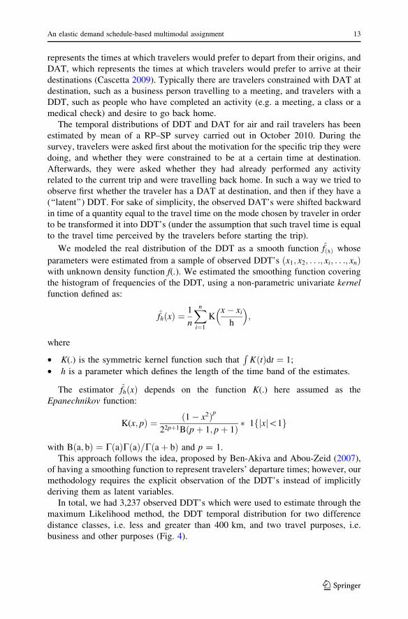
We modeled the real distribution of the DDT as a smooth function fðxÞ whose
parameters were estimated from a sample of observed DDT’s ðx1; x2; . . .; xi; . . .; xnÞwith unknown density function f(.). We estimated the smoothing function covering
the histogram of frequencies of the DDT, using a non-parametric univariate kernelfunction defined as:
fhðxÞ ¼1
n
Xn
i¼1
Kx� xi
h
� �;
where
• K(.) is the symmetric kernel function such thatR
KðtÞdt ¼ 1;
• h is a parameter which defines the length of the time band of the estimates.
The estimator fhðxÞ depends on the function K(.) here assumed as the
Epanechnikov function:
K(x; pÞ ¼ 1� x2ð Þp
22pþ1B pþ 1; pþ 1ð Þ � 1 xj j\1f g
with B a; bð Þ ¼ CðaÞCðaÞ=Cðaþ bÞ and p = 1.
This approach follows the idea, proposed by Ben-Akiva and Abou-Zeid (2007),
of having a smoothing function to represent travelers’ departure times; however, our
methodology requires the explicit observation of the DDT’s instead of implicitly
deriving them as latent variables.
In total, we had 3,237 observed DDT’s which were used to estimate through the
maximum Likelihood method, the DDT temporal distribution for two difference
distance classes, i.e. less and greater than 400 km, and two travel purposes, i.e.
business and other purposes (Fig. 4).
An elastic demand schedule-based multimodal assignment 13
123

The joint mode/service/run choice model
The joint mode/service/run choice model simulates the distribution of demand flows
among the modes, the services and the runs available on a given OD pair using a
random utility discrete choice model (Ben-Akiva and Lerman 1985). The use of
such model requires the definition of the choice set, the selection of a specific model
structure according to the expected correlation among the utilities of the alternatives
(e.g. logit, nested-logit, etc.); the selection of a number of significant variables
affecting the choice (i.e. the attributes), and the estimation of the parameters of each
attribute.
Choice set
In principle, the modes/services/runs alternatives on a given OD pair (i.e. the choice
set) derive from the combination of all the modes, services and runs available. This
would lead to a choice set including the Auto, all the available flights, all the
available HSR trains offered by Trenitalia (i.e. the national incumbent), all those
offered by NTV (i.e. the new HSR operator) and all the intercity trains, on the given
OD. Moreover, for Air and Rail (Intercity, HSR-Trenitalia, HSR-NTV), the
available runs should be distinguished by class (1st and 2nd) and by departure time.
Such a big number of alternatives would not be manageable and could possibly be
unrealistic. Therefore, the definition of a limited choice set for each group of
travelers (market segment) is needed to avoid unrealistic choice context. To this
aim, we derived the choice set from some reasonable assumptions and checked the
biases such assumption might induce, using the observed choices in the sample
(aggregate calibration of the choice set generation model).
Fig. 4 The estimated desired departure time (DDT) distribution by distance class and travel purpose
14 E. Cascetta, P. Coppola
123
Firstly, we assumed that air mode is not available for OD pair at a distance less
than 400 km and auto is not available for travelers who do not own a car. Secondly,
air and rail services were subjected to further assumptions on the number of runs to
be included in the choice set based on maximum earliness/lateness bands and on
dominance rules. The introduction of such rules to limit the number of the available
alternatives might lead to some biases in the demand forecasts, due to the fact that in
some cases we force travelers to exclude runs (e.g. those departing too much early
and too much late with respect to the DAT) which they actually might take into
consideration. The results could be an over-estimation of the demand on the runs in
the period of the day with high-frequency service (i.e. peak period) if we limit the
choice set to the first runs before and after the DDT. In fact, in such case, thanks to
the high frequency of the service, travelers may consider to take into consideration
also runs departing after the first available (i.e. with short additional waiting times).
On the other hand, the results could be an under-estimation of the traffic on the runs
in the peak periods, if we limit the choice set by including all the runs within a pre-
specified time band; in this case the model would spread the travelers over a big
number of runs (due to the high frequency in the peak period) before and after the
DDT, whereas in the reality travelers may consider only the first or the second best
available alternatives.
To avoid the above biases introduced by the way the number of elemental paths
between each OD pair is limited, different heuristic rules were tested by computing
the respective ‘‘coverage ratio’’ (i.e. the percentage of cases in which the observed
run actually chosen belongs to the choice set generated by a given rule) based on a
sample of 1,884 travelers gathered during an RP–SP survey carried out in October
2010.
The first rule tested was that of considering available for each service (air,
intercity, HSR-Trenitalia and HSR-NTV) only two runs, namely the first ‘‘early’’
and the first ‘‘late’’ trip with respect to the DDT of each traveler. The resulting
coverage ratios were about 77 % for air, 64 % for intercity and HSR Trenitalia and
59 % for HSR-NTV services.
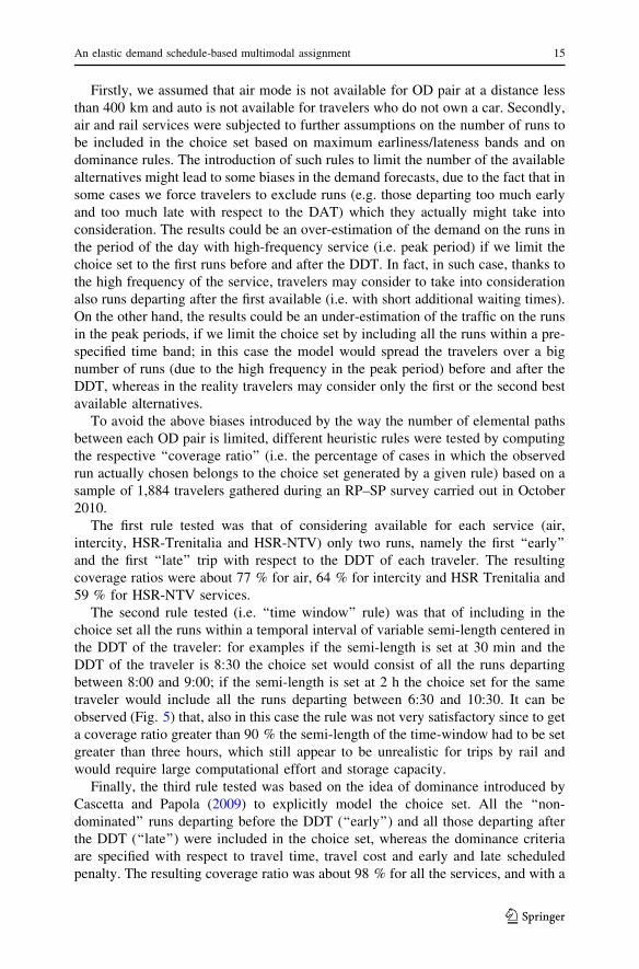
The second rule tested (i.e. ‘‘time window’’ rule) was that of including in the
choice set all the runs within a temporal interval of variable semi-length centered in
the DDT of the traveler: for examples if the semi-length is set at 30 min and the
DDT of the traveler is 8:30 the choice set would consist of all the runs departing
between 8:00 and 9:00; if the semi-length is set at 2 h the choice set for the same
traveler would include all the runs departing between 6:30 and 10:30. It can be
observed (Fig. 5) that, also in this case the rule was not very satisfactory since to get
a coverage ratio greater than 90 % the semi-length of the time-window had to be set
greater than three hours, which still appear to be unrealistic for trips by rail and
would require large computational effort and storage capacity.
Finally, the third rule tested was based on the idea of dominance introduced by
Cascetta and Papola (2009) to explicitly model the choice set. All the ‘‘non-
dominated’’ runs departing before the DDT (‘‘early’’) and all those departing after
the DDT (‘‘late’’) were included in the choice set, whereas the dominance criteria
are specified with respect to travel time, travel cost and early and late scheduled
penalty. The resulting coverage ratio was about 98 % for all the services, and with a
An elastic demand schedule-based multimodal assignment 15
123

number of generated diachronic paths equal only to the 35 % of the number
generated with the time bands needed to get a comparable coverage ratio. In other
terms, the number of path in a time window that guarantees a given coverage ratio is
much higher than the number of non-dominated paths with the same coverage ratio.
The non-dominance rule was applied for the generation of mode/service/run choice
set in the assignment model.
Choice model structure
Random utility models were used to simulate travelers’ choices. In such models,
each traveler is assumed to associate an utility, Uj, to each alternative j of his/her
choice set C and to choose the maximum utility alternative. According to the joint
distribution of random variables, Uj, the probability of choosing the generic
alternative j, p[j|C], assumes different forms, both closed (logit, nested logit, etc.)
and non-closed (probit, hybrid logit, etc.). A nested logit model is here adopted.
This introduces a tree correlation structure among alternatives in the choice set and
its analytical expression is the following (Cascetta 2009):
p jjC½ � ¼exp Vj=ha jð Þ� �
exp Yoð Þ �Pr2Ajexp dr � 1ð ÞYr½ � j 2 C
where a Gumbel parameter, hr, and an utility, Ur, is associated to each intermediate
(structural) node r of the choice tree (Fig. 6). Vr, which is the expected value of Ur,is proportional to Yr, which represents the expected maximum perceived utility
(EMPU) among all alternatives contained in nest r. Aj is the set of all ancestor nodes
of j except the root node o (Aj : a(j), a(a(j)),…) and dr represents the ratio between
hr and ha(r), i.e. the Gumbel parameters associated respectively to node r and its
ancestor a(r). This parameter falls within the range [0-1] (i.e. 0 B dr B 1) and
reproduces the correlation among the alternatives belonging to nest r. Indeed dr = 1
Fig. 5 Coverage ratio of the ‘‘time window’’ rule tested to generate the paths choice set
16 E. Cascetta, P. Coppola
123

means that all alternatives belonging to nest r are uncorrelated (i.e. perceived as
independent). if dr = 1 Vr the nested logit specification results in a logit one; dr = 0
means that alternatives belonging to nest r are treated as completely correlated. In
the latter case, the choice among the alternatives becomes deterministic and the
systematic utility of node r, Vr, coincides with the maximum systematic utility
among these alternatives.
In our case, the model has a multi-level tree structure with intermediate nodes
corresponding to (Fig. 7):
• Main modes (auto, air, rail)
• Rail service (intercity and HSR)
• HSR Operator (Trenitalia and NTV)
• Service class (1st and 2nd)
With respect to the attributes, the classic attributes Xkj used to simulate the modal
choice (i.e. socio-economic attributes of the traveler and l.o.s. attributes) plus the
early-departure/late-arrival penalties were included in a linear form in the
systematic utility functions:
Vj Xj
� �¼X
k
bkXkj
Fig. 6 Choice tree of amultilevel nested logit structure
Fig. 7 Nested structure of the schedule-based mode/service/operator/class/run choice model
An elastic demand schedule-based multimodal assignment 17
123
Data set
The available database refers to ex-province trips between all the provinces served
by the HSR service (see the ‘‘in-scope’’ area in Fig. 2), gathered by a RP–SP survey
carried on during October 2010. The sample of travelers was obtained by stratified
random sampling, with 36 strata defined by: 2 travel purposes (business and other
purposes), 3 distance classes (\100 km; between 100 and 400 km, [400 km), 3
main modes (auto, air, rail), 2 city-types as origin zone, i.e. city with or without a
HSR station.
The RP part of the interview (i.e. the recruiting questionnaire) concerns, first,
some socio-economic characteristics of the traveler and, then, some information
related to the last ex-province trips carried out in the previous 3 months (if any),
such as: trip purpose, origin, destination, departure time, arrival time and the modes
and the services used to arrive at destination, the departure and arrival time of the
chosen service trip as well as the desired departure or arrival time at destination, as
previously described (see Sect. 3.2). The sample from the panel was enriched by
observations gathered at the HSR stations and the airports in the study area. Among
the total number of travelers recruited in the RP survey (1,332 recruited from the
population, 385 at the airports and 1,633 at the HSR stations), 445 accepted to go on
with the SP part of the survey, consisting of 6 scenarios conceived to test:
• fare levels;
• L.o.S. attributes (travel time ? access/egress);
• Run departure times;
• HSR operator (i.e. brand effect).
The SP database resulted in about 1,884 observations. Table 3 reports a summary
of the choices and availabilities of each alternative in the sample.
Model estimation
The models were estimated using the maximum likelihood method. Several nested
structures to simulate the joint mode/service/run choice were estimated for two
trip purposes (i.e. ‘‘Business’’ and ‘‘Other purposes’’). In the current model
Table 3 Mode chosen, availability and other statistics from the SP database
Auto Intercity
Trenitalia
HSR
Trenitalia
HSR
NTV
Air Total
Mode chosen 143 380 683 540 138 1,884
Mode availability 1,790
(99.7 %)
393
(21 %)
1,656
(88 %)
1,299
(69 %)
635
(34 %)
–
Average in-vehicle time (min) 305 267 145 150 73 –
Average access time (min) – 60 69 73 101 –
Average egress time (min) – 63 68 72 85 –
Average travel cost (€) 71 43 62 – 127 –
18 E. Cascetta, P. Coppola
123
specification, the following attributes of the systematic utility of the alternatives
resulted to be statistically significant:
• Travel time (generic)
• Travel cost, distinguished by four categories of travelers: traveling alone by car,
traveling in group by car, reimbursed and not reimbursed of travel expenses
(when traveling by air or by rail);
• Access/egress time, for air and rail services;
• Early schedule delay w.r.t. DDT, for air and rail services;
• Late schedule delay w.r.t. DDT, for air and rail services;
• a dummy ‘‘male’’ in the systematic utility of the auto;
• a dummy for ‘‘priority gate’’ at the airport to speed up the control procedure for
certain destinations;
The nesting structure consists of three independent nests for air runs, Trenitalia
runs (intercity and HSR using 1st and 2nd class services) and NTV runs (1st and 2nd
class). The estimation results are reported in Table 4 together with some statistics
on the parameters and goodness of fit.
As it can be seen, the goodness-of-fit improves after the segmentation by travel
purpose. For Business all the b parameters are significant at a level greater than
95 %. For Other purposes, the parameters of the cost for Intercity, HSR and air
result to be not significant if travel expenses are reimbursed. These results confirm
the fact that cost plays a minor role in the choice of mode/service when the travel
expenses are reimbursed. Moreover, the beta of the travel time results to be
significant at a level of confidence of 85 % for ‘‘other-purposes’’ trips and the
dummy related to the priority gate at the airport is not significant at all, while it is
significant and equivalent to 18 min of travel time for business trips.
The lower value of beta of the travel cost by auto when traveling in group w.r.t.
traveling alone reproduces the fact that, on the average, using the car allows
travelers to share the costs; for Business trips the value of bcar_cost_alore and
bcar_cost_group are not statistically different whereas, for ‘‘other-purposes’’ trips, the
ratio between the value of bcar_cost_alore and bcar_cost_group is about 1.4 which is
comparable to average car occupancy for ex-urban trips.
The ratio between the beta coefficients related to the cost (for the above four
categories of travelers) and that of the travel time is an estimate of the value of time
(VOT), indicating how much the user is willing to pay in order to save a unit of
time. In particular, the VOT by car ranges between 10 and 15 Euro/h, while the
VOT’s of other modes (rail and air) ranges between 25 and 70 Euro/h depending on
the typology of the service, the travel purpose and whether the travel cost is
reimbursed or not (Table 5). These values are comparable with those obtained in
other similar studies: for instance, Roman et al. (2007) estimate VOT’s ranging
from 14 to 65 Euro/h for HSR in Spain (differentiated for different phase of the
trips: access/egress, on board, waiting, delay); Yao and Morikawa (2005) estimate a
VOT of 59.7 Euro/h for business trips (not distinguishing by reimbursed and not-
reimbursed travelers) and of 21 Euro/h for other-purposes trips.
In addition to the level of service attributes, a set of Alternative Specific
Constants (ASC) has been included in the model specification. These have been
An elastic demand schedule-based multimodal assignment 19
123

differentiated by mode, distance class (i.e. [400 and \400 km), service class (1st
and 2nd) and for HSR operator (Trenitalia and NTV). It is interesting to point out
that the difference of the ASC of NTV minus those of Trenitalia are always negative
(Table 6): larger difference for 1st class service and on the short distance
Table 4 Model parameters and statistics
All Business Other purposes
b Value (t test) Value (t test) Value (t test)
Access Egress time (min) -0.00805 (-5.25) -0.00555 (-2.13) -0.0103 (-5.09)
Travel time (min) -0.00700 (-4.89) -0.0133 (-5.82) -0.0054 (-1.51)a
Early schedule delay (min) -0.00467 (-4.52) -0.00188 (-1.39) -0.00677 (-4.13)
Late schedule delay (min) -0.00917 (-19.27) -0.0130 (-16.2) -0.00617 (-10.90)
Cost by auto if travel in group (Euro) -0.0292 (-4.52) -0.0524 (-2.69) -0.0295 (-2.08)
Cost by auto if travel alone (Euro) -0.0386 (-5.56) -0.0527 (-3.76) -0.0405 (-4.14)
Cost by intercity if reimbursed (Euro) -0.0247 (-1.88) -0.0158 (-2.73) b
Cost by intercity if NOT reimbursed (Euro) -0.022 (-5.13) -0.0377 (-3.50) -0.0172 (-3.45)
Cost by HSR if reimbursed (Euro) -0.00857 (-1.42)a -0.0120 (-4.11) b
Cost by HSR if NOT reimbursed (Euro) -0.0156 (-10.90) -0.0284 (-11.1) -0.00256 (-2.04)
Cost by Air if reimbursed (Euro) -0.0079 (-1.48)a -0.0109 (-1.91) b
Cost by Air if NOT reimbursed (Euro) -0.0150 (-7.15) -0.0201 (-5.65) -0.0194 (-5.21)
Dummy male (1/0) ?0.406 (1.91) ?1.400 (2.41) ?0.550 (2.28)
Dummy priority gate at the airport (1/0) ?0.194 (0.97)b ?0.242 (1.97) b
Tetha_Air ?0.915 (1.15)b ?0.921 (1.65)a ?0.904 (1.21)b
Tetha_Trenitalia ?0.806 (1.11)b ?0.840 (2.51) ?0.750 (1.28)b
Tetha_NTV ?0.894 (1.27)b ?0.882 (2.87) ?0770 (1.38)b
Rho-square 0.154 0.161 0.218
Adjusted rho-square 0.150 0.153 0.209
Final log-likelihood -5,341.875 -3,006.045 -2,137.475
Initial log-likelihood -6,317.116 -3,583.503 -2,733.613
Sample size 1,884 1,067 817
a Significant at level of 85 %, b parameter not statistically significant
Table 5 Estimated values of time (VOT’s) by travel purposes
All purposes Business Other purposes
Cost by auto if travel in group (euro/h) 14.4 15.2 11.0
Cost by auto if travel alone (euro/h) 10.9 15.1 8.0
Cost by Intercity if reimbursed (euro/h) 17.0 50.5
Cost by Intercity if NOT reimbursed (euro/h) 19.1 21.2 18.8
Cost by HSR if reimbursed (euro/h) 49.0 66.5
Cost by HSR if NOT reimbursed (euro/h) 26.9 28.1 12.7
Cost by air if reimbursed (euro/h) 53.2 73.2
Cost by air if NOT reimbursed (euro/h) 28.0 39.7 16.7
20 E. Cascetta, P. Coppola
123
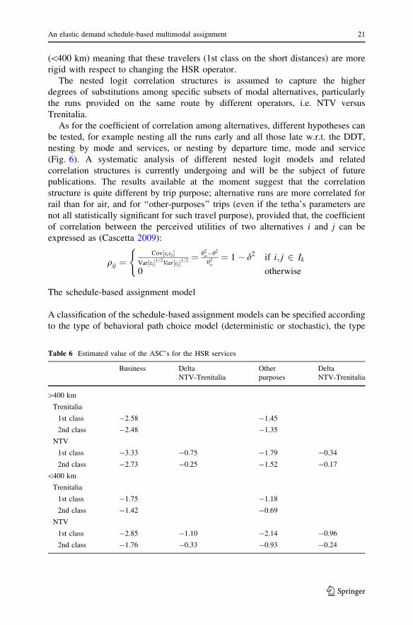
(\400 km) meaning that these travelers (1st class on the short distances) are more
rigid with respect to changing the HSR operator.
The nested logit correlation structures is assumed to capture the higher
degrees of substitutions among specific subsets of modal alternatives, particularly
the runs provided on the same route by different operators, i.e. NTV versus
Trenitalia.
As for the coefficient of correlation among alternatives, different hypotheses can
be tested, for example nesting all the runs early and all those late w.r.t. the DDT,
nesting by mode and services, or nesting by departure time, mode and service
(Fig. 6). A systematic analysis of different nested logit models and related
correlation structures is currently undergoing and will be the subject of future
publications. The results available at the moment suggest that the correlation
structure is quite different by trip purpose; alternative runs are more correlated for
rail than for air, and for ‘‘other-purposes’’ trips (even if the tetha’s parameters are
not all statistically significant for such travel purpose), provided that, the coefficient
of correlation between the perceived utilities of two alternatives i and j can be
expressed as (Cascetta 2009):
qij ¼Cov½eiej�
Var½ei�1=2Var½ej�1=2 ¼ h2o�h2
h2o
¼ 1� d2 if i; j 2 Ik
0 otherwise
(
The schedule-based assignment model
A classification of the schedule-based assignment models can be specified according
to the type of behavioral path choice model (deterministic or stochastic), the type
Table 6 Estimated value of the ASC’s for the HSR services
Business Delta
NTV-Trenitalia
Other
purposes
Delta
NTV-Trenitalia
[400 km
Trenitalia
1st class -2.58 -1.45
2nd class -2.48 -1.35
NTV
1st class -3.33 -0.75 -1.79 -0.34
2nd class -2.73 -0.25 -1.52 -0.17
\400 km
Trenitalia
1st class -1.75 -1.18
2nd class -1.42 -0.69
NTV
1st class -2.85 -1.10 -2.14 -0.96
2nd class -1.76 -0.33 -0.93 -0.24
An elastic demand schedule-based multimodal assignment 21
123

link performance functions (flow-dependent or flow-independent, i.e. uncongested
or congested networks), the assignment approach (network loading, user equilib-
rium, dynamic process), and the dynamic evolution (within-day and/or day-to-day)
they take into account (Cascetta 2009).
In the case of low frequency and uncongested public transportation networks, a
dynamic network loading (DNL) model can be used; in this case, the option of
deterministic or stochastic path choice model can be considered: an exhaustive
review of such models is reported in Wilson and Nuzzolo (2004). In our case study,
a stochastic network loading model with no capacity constrains was adopted to
estimate the flows on the links of the diachronic network, i.e. the flows on individual
trains.
Model validation
The overall elastic demand assignment model was first validated by comparing the
assigned daily flows on each station-to-station segment of the HSR network (e.g. the
rail segment Rome–Naples) and the estimated flows on that segment by counts
(Fig. 8). It can be observed that the rho square is 0.95 and the percentage error for
single segment is within 10–20 %.
Furthermore, for each segment, we compared the assigned flows on-board each
high speed train predicted by the model and the counted flows in a working day of
October 2010. The scatter diagram predicted versus counted is reported in Fig. 9. It
can be seen that, as expected, the order of magnitude of the prediction error
increases, e.g. the rho squared is 0.48. However, the dispersion around the bisector
of the scatter diagram is comparable to that observed in the regression plotted out
Fig. 8 Scatter diagram of predicted versus counted average daily flows (on October 2010) by HSRsegment
22 E. Cascetta, P. Coppola
123

using the counted flows in May and October 2010 (Fig. 10); here the rho squared
resulted to be equal to 0.51. In other terms, the error of the model is within the day-
to-day variability of the observed train flows on the HSR links.
Fig. 9 Scatter diagram of predicted versus counted daily flows on board the high speed trains (onOctober 2010)
Fig. 10 Scatter diagram of counted daily flows on high speed trains on May 2010 versus October 2010
An elastic demand schedule-based multimodal assignment 23
123
Some applications to fares and timetable design
In Italy, the first HSR service was launched in 1992 between Firenze and Roma with
the so called ‘‘direttissima’’, allowing trains to run at 230 km/h and covering
254 km in about 2 h. Today the HSR service includes several city pairs at distances
in between 100 and 250 km, e.g. Roma–Napoli (205 km in 1 h and 10 min),
Milano–Torino (125 km in 52 min) and Roma–Milano with a direct service
covering 515 Kilometers in 3 h with a service frequency on the HSR network ranges
from 1 to 4 trains/h in the peak period on the rail segments between Roma, Firenze
and Bologna (Fig. 2).
The modeling architecture presented in this paper has been applied to predict the
impacts on national passenger volumes due to the incoming of the new operator
NTV starting from year 2012. Different hypothetical scenarios have been tested
under different macroeconomic assumptions and marketing strategies of the HSR
competitors on the long distance (i.e. NTV vs. Trenitalia).
It should be stressed that reference and alternative scenarios reported in the
following are hypothetical and do not represent commercial choices made by both
NTV and Trenitalia operators.
Reference scenario
In the reference scenario it was assumed that the NTV service network reproduced
the structure of Trenitalia services. Assuming the 2010 as base-year, the reference
scenario (year 2012) with the NTV service fully operative shows an increase of
passenger-Km of 9.2 % w.r.t. 2010 with a split between NTV and Trenitalia,
respectively, of 33.4 and 66.6 %. Given an overall demand growth between 2010
and 2012 of 3.3 %, a net increase of demand due to the additional HSR services by
NTV of a significant 5.9 % can be estimated, representing the sum of the induced
and diverted demand at year 2012 caused by the increase of HSR frequencies.
HSR fares and timetable setting
The applications here presented regard some potential operational policies of the
new operator NTV, such as the variation of the fares (scenario 1) and the
optimization of the timetables to increase passenger flows (scenario 2).
In scenario 1, two hypotheses on the HSR fares have been tested starting from a
reference case: Case 1) Trenitalia reduces the HSR fares of 20 %; Case 2) both the
HSR operators reduce the fares by 20 % w.r.t. reference case (Table 7). In the first
case, Trenitalia market share increases of 13.2 % and conversely NTV market share
reduces of 10.1 %; the HSR overall demand increases of 5.4 %. In the second case,
the overall HSR demand increases of 7.3 % while the HSR market shares of
Trenitalia increases of 8.2 % whereas NTV market share increases of 5.4 %. This
allows us to estimate some direct and cross (HSR demand) arc-elasticity’s to HSR fares.
In particular, it can be estimated a direct elasticity of total HSR demand w.r.t. fares of
-0.37 and a HSR operators cross-elasticity of ?0.74 (i.e. a fare reduction by one
operator induce a decrease of traffic on the other competing operator). Higher values of
24 E. Cascetta, P. Coppola
123
cross operators elasticity’s than modal elasticity’s are to be expected given the
correlation structure of the perceived utility according to the nested structure of Fig. 7.
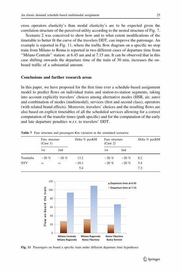
Scenario 2 was conceived to show how and to what extent modifications of the
timetable to better fit the curve of the travelers DDT, can improve the patronage. An
example is reported in Fig. 11, where the traffic flow diagram on a specific no stop
train from Milano to Roma is reported in two different cases of departure time from
‘‘Milano Centrale’’ station: at 6.45 am and at 7.15 am. It can be observed that in this
case shifting onwards the departure time of the train of 30 min, increases the on-
board traffic of a substantial amount.
Conclusions and further research areas
In this paper, we have proposed for the first time ever a schedule-based assignment
model to predict flows on individual trains and station-to-station segments, taking
into account explicitly travelers’ choices among alternative modes (HSR, air, auto)
and combination of modes (multimodal), services (first and second class), operators
(with related brand effects). Moreover, travelers’ choices and the resulting flows are
also based on explicit timetables of all the scheduled services allowing for a correct
computation of the transfer times (path specific) and for the computation of the early
and late departure penalties w.r.t. to travelers‘ DDT.
Table 7 Fare structure and passengers-Km variation in the simulated scenarios
Fare structure
(Case 1)
Delta % paxKM Fare structure
(Case 2)
Delta % paxKM
1st 2nd 1st 2nd
Trenitalia -20 % -20 % 13.2 -20 % -20 % 8.2
NTV = = -10.1 -20 % -20 % 5.4
5.4 7.3
Fig. 11 Passengers on board a specific train under different departure time hypotheses
An elastic demand schedule-based multimodal assignment 25
123

The OD flows on the HSR services have been assigned to individual trains
allowing the forecasting of occupancies on each train on each station-to-station link.
The error of the model has resulted to be within the day-to-day range of variability
of the flows. This has validated the model as a support tool for HSR operators to
simulate operational strategies for HSR demand forecasting and in general for
railways marketing, such as optimal timetable setting and differentiated fare
structures (e.g. by time of day, or by yield management). Moreover, as part of a
more comprehensive modeling architecture integrating models forecasting the
induced demand and the economy-related demand growth, the proposed approach
allows to better estimate also the long-term (strategic) impacts of HSR, by
computing in a more precise way, the alternative paths on the multimodal/
multiservice network (choice set), and some relevant attributes such as the transfer
times from mode to mode, or service to service, which play an important role in the
choice of the available alternatives and which are typically computed on a daily
average basis (e.g. in the traditional frequency-based models). In this respect, the
adopted schedule-based approach, can be considered as an extension of the models
proposed in the literature.
The mode-service-operator-run choice models have been estimated using a
dataset of RP–SP interviews gathered in October 2010. The estimated values of time
(VOT) and elasticity’s resulted to be comparable with those obtained in other
similar studies. In particular, our VOT’s on Rail and Air ranges between 25 and 70
Euro/h depending on the typology of the service, the travel purpose and whether the
travel costs are reimbursed or not reimbursed. The (arc) direct elasticity’s of HSR
demand with respect to HSR fares is -0.37, and a value of ?0.74 of cross
elasticity’s w.r.t. the fares of competing HSR operator have been estimated.
A nested logit correlation structures has been assumed to capture the higher
degrees of substitutions among specific subsets of mode/service/run alternatives,
particularly the runs provided on the same route by different operators. In this
respect different hypotheses can be tested, for example nesting all the runs early and
all those late w.r.t. the DDT, nesting by mode and services, or nesting by departure
time, mode and service. A systematic analysis of different nested logit models and
related correlation structures is currently undergoing and will be the subject of
future publications. The results available at the moment suggest that the correlation
structure is quite different by trip purpose; alternative runs are more correlated for
rail than for air, and for ‘‘Other-purposes’’ trips (even if the tetha’s parameters
resulted to be not all statistically significant for such travel purpose).
Acknowledgments The authors wish to thank the NTV and Net Engineering companies in the person of
Giuseppe Bonollo and Vito Velardi for providing the access to the data, based on which the models have
been estimated, and Roberto Dall’Alba for computing the l.o.s. attributes and for the assistance in
elaborating the database.
References
Ahuja RK, Magnanti TL, Orlin JB (1993) Network flows. Theory, algorithms and applications. Prentice
Hall, New Jersey
26 E. Cascetta, P. Coppola
123
Anez J, de la Barra T, Perez B (1996) Dual graph representation of transport networks. Transp Res B
30:209–216
Ben-Akiva M, Abou-Zeid M (2007) Methodological issues in modeling time-of-travel preferences. In:
Proceedings of the World Conference of Transportation Research (WCTR), Lisbon, Portugal
Ben-Akiva M, Lerman S (1985) Discrete choice analysis. MIT Press, Cambridge
Ben-Akiva M, Cascetta E, Coppola P, Papola A, Velardi V (2010) High speed rail demand forecasting in
a competitive market: the Italian case study. In: Proceedings of the World Conference of
Transportation Research (WCTR), Lisbon, Portugal
Cascetta E (2009) Transportation systems analysis: models and applications. 2nd edn. Springer, Berlin
Cascetta E, Coppola P (2011) High speed rail demand: empirical and modeling evidences from Italy. In:
Proceedings of the European Transport Conference (ETC.), Glasgow, UK
Cascetta E, Papola A (2009) Dominance among alternatives in random utility models. Transp Res A
43(2):170–179
Couto A, Graham DJ (2008) The impact of high-speed technology on railway demand. Transportation
35:111–128
Froidh O (2005) Market effects of regional high-speed trains on the Svealand line. J Transp Geogr
13:352–361
Froidh O (2008) Perspectives for a future high-speed train in the Swedish domestic travel market.
J Transp Geogr 16(4):268–277
Hsu C, Chung W (1997) A model for market share distribution between high-speed and conventional rail
services in a transportation corridor. Ann Reg Sci 31:121–153
Ivan D (2011) High speed rail—urbanization triggering demand for mass transit Frost & Sullivan Market
Insight
Mandel B, Gaudry M, Rothengatter W (1997) A disaggregate Box-Cox Logit mode choice model of
intercity passenger travel in Germany and its implications for high-speed rail demand forecasts. Ann
Reg Sci 31:99–120
Martin JC, Nombela G (2007) Microeconomic impacts of investments in high speed trains in Spain. Ann
Reg Sci 41:715–733
Nuzzolo A, Russo F (1993) Un modello di rete diacronica per l’assegnazione dinamica al trasporto
collettivo extraurbano. Ricerca Operativa 67:37–56
Park Y, Ha H-K (2006) Analysis of the impact of high-speed railroad service on air transport demand.
Transp Res E 42(2):95–104
Roman C, Espino R, Martin C (2007) Competition of high-speed train with air transport: the case of
Madrid–Barcelona. J Air Transp Manag 13:277–284
Tong CO, Richardson AJ (1984) Estimation of time-dependent origin-destination matrices for transit
networks. J Adv Transp 18:145–161
Wardman M (2006) Demand for rail travel and the effects of external factors. Transp Res E
42(3):129–148
Wilson NHM, Nuzzolo A (2004) Schedule-based dynamic transit modeling: theory and applications.
Kluwer Academic Publisher, Dordrecht
Wong SC, Tong CO (1999) A stochastic transit assignment model using a dynamic schedule-based
network. Transp Res B 33:107–121
Yao E, Morikawa T (2005) A study of an integrated intercity travel demand model. Transp Res A
39(4):367–381
An elastic demand schedule-based multimodal assignment 27
123


![Monitoria multimodal cerebral multimodal monitoring[2]](https://static.fdocuments.in/doc/165x107/552957004a79599a158b46fd/monitoria-multimodal-cerebral-multimodal-monitoring2.jpg)