Diaphragm Behavior of Floor Systems and Its Effect on Seismic Building Response

AN ELASTIC ANALYSIS OF A CANTILEVER SLAB PANEL

SUBJECTED TO AN IN-PLANE END SHEAR

by

Zhensheng Wu

Ti Huang

This work has been carried out as part of an investigation sponsored by the National Science Foundation.

Any opinions, findings, and conclusions or recommendations expressed in this publication are those of the authors and do not necessarily reflect the views of the Sponsor or Fritz Engineering Laboratory, Lehigh University, Bethlehem, Pennsylvania.

Department of Civil Engineering

Fritz Engineering Laboratory Lehigh University

Bethlehem, Pennsylvania

May, 1983 Fritz Engineering Laboratory Report No. 481.1

TABLE OF CONTENTS

ABSTRACT iv

I. INTRODUCTION 1

II. SOLUTION OF THE BENDING DISPLACEMENT 3

III. SIMPLIFICATION OF THE BENDING SOLUTION 11

IV. EXAMPLES 14

v. CONCLUSIONS 17

VI. REFERENCES 18

VII. TABLES 19

VIII. FIGURES 21

IX. ACKNOWLEDGMENTS 25

iii

ABSTRACT

An analytical solution is presented for the elastic

response of a slab panel subjected to an in-plane end shear.

The loading condition is separated into a pure shear component

and an essentially bending component. Simplified approximations

are provided and example applications are included.

iv

I. INTRODUCTION

In a building structure containing several lateral load resisting

systems, the floor systems act as diaphragms connecting these vertical

systems and control the distribution of lateral load among the several

parallel systems. The basic behavior of a floor panel under such a con­

dition may be taken to be that of a cantilever deep beam subjected to a

distributed shear load on its free end as shown in Fig. 1a. Because of

the geomet_ry of the panel, where the planar dimensions B and H are typi­

cally of the same order of magnitude, and the thickness is much smaller,

a satisfactory analysis cannot be achieved by the conventional methods

of strength of materials. This report presents an analytical solution

based on a separation of the shear and bending effects.

The distribution of the shear load T at the end of the floor slab

panel is generally not known. In the proposed solution, a uniform dis­

tribution is initially assumed, considering that the loading is typi­

cally induced either by inertia (as in the case of earthquake) or rela­

tive displacement between the connected vertical systems. It is then

possible to resolve the present problem into two component parts, as

shown in Fig. 1b and 1c. The first component, shown in Fig. 1b, repre­

sents a pure shear condition. For a member of uniform thickness,

T = 0

and

!::. = s

where

T Bt

T TH ....£H = GBt G

T = Uniform shearing stress in the member 0

t = Thickness of slab

G = Shear modulus of elasticity

(1-1)

(1-2)

The second component of the load, shown in Fig. 1c,causes the slab

panel to deform in an essentially "bending" mode. The free end displace­

ment caused by this load, ~' will be referred to as the "bending

1

displacement" in this report. The solution for ~ is presented in the

next section. It is clear that the total deflection ~ in Fig. la can

be obtained by superposition.

(1-3)

It should be pointed out that a conceptual difference exists bet­

ween the shear and bending displacements defined here and those commonly

found in literature on mechanics of materials. In the later case, the

two components are caused by the same load, but are derived from the

separate (but coexisting) strain components. Here, they refer to sepa­

rate loading conditions.

2

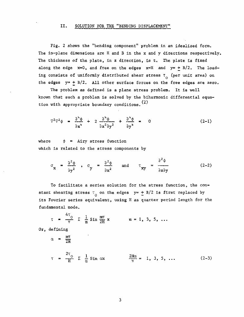
II. SOLUTION FOR THE "BENDING DISPLACEMENT"

Fig. 2 shows the "bending component" problem in an idealized form.

The in-plane dimensions are H and B in the x and y directions respectively.

The thickness of the plate, in z direction, is t. The plate is fixed

along the edge x=O, and free on the edges x=H and y= ~ B/2. The load­

ing consists of uniformly distributed shear stress T0

(per unit area) on

the edges y= ~ B/2. All other surface forces on the free edges are zero.

The problem as defined is a plane stress problem. It is well

known that such a problem is solved by the biharmonic differential equa­

tion with appropriate boundary conditions. (2)

= 2

where ~ = Airy stress function

which is related to the stress components by

cr X

= cr y

= and T xy

0 (2-1)

= (2-2) axay

To facilitate a series solution for the stress function, the con­

stant shearing stress T0

on the edges y= ~ B/2 is first replaced by

its Fourier series equivalent, using H as quarter period length for the

fundamental mode.

4T 1 m'IT 0 l: T = -- -Sin- X 'IT m 2H m = 1, 3, 5, •••

Or, defining

mrr Cl. = 2H

2T 1 s· 0

l: T = H - ~n CI.X Cl.

2Ha --= 'IT

1, 3, 5, •.• (2-3)

3

The selection of H for quarter period length is necessary to satisfy

the boundary conditions, as will be shown later.

It is now appropriate to suggest the following solution for the

stress function:

<P = l:¢ = a 1 l: - Cos axf (y) a a (2-4)

where e~ch <Pa satisfies the biharmonic equation (2-1) separately. Solu­

tion of the biharmonic equation leads to:

f (y) a =

From Equation (2-2)

a = l: ..!:.. Cosaxf" (y) x a a

a = - l:a Cosaxf (y) Y a

The stress field in the member is skew-symmetric with respect to the

x-axis, i.e.,

a = -a (-y) x(y) x

T (y) = T (-y) xy xy

Consequently, f~ (y) must be odd functions of y, and f~(y) must be even.

Hence, = = o.

4

The general solution of this problem is, therefore, as follows:

¢ =

cr = X

cr = y

T = xy

(2-5)

(2-6)

(2-7)

(2-8)

In equations (2-5) through (2-8), the summations are over the values of

a such that

2Ha -- = m = 1, 3, 5, •••

'IT

The coefficients c 2 and c 3 are determined by the boundary stress con­

ditions on y= ~ B/2, where

cr = o y

T = T xy

Substituting Equations (2-3), (2-7) and (2-8), and equating the corres­

ponding terms of each series

aB B . aB 1 aB c 2cosh z- + c3 { 2 S~nh z- + a Cosh z- }

Solving these equations for c 2 and c 3

4T 0

=- aH

B aB 2 Cosh z-aB - SinhaB

S . h aB ~n- z-

aB - SinhaB

5

Substituting into the general solutions (2-5) through (2-8)

B aB aB 4-r

0 1 ~osh 2 Sinhay - Sinh 2-"f Cosh ay = --- I -- Cosax ------~~--~~~~--~----------H 2 aB - SinhaB a

(2-9)

4 B C haB Si h S' h aB C h 2 s· h aB s· h T 2 OS 2 n ay - ~n z-Y OS ay - a ~n z- ~n ay cr

X

cr X

T xy

= ---0

I Cosax ~----~------~--~~--~--------~~----~-------H an - Sinh aB

4-r ~osh ~B Sinhay aB

0 Co sax Sinh z- yCoshay

(2-11) = - - I H aB - Siuh aB

4T B aB aB Sinhay - ~inh ~B Coshay 2 Cosh z- Coshay Sinh z-Y

= __.£I Sin ax H aB - Sinh aB

m'IT Along the end boundary x=H, ax= z-· Therefore, form= 1, 3, 5, ••• ,

cos ax= O, and sin ax= +1. The boundary stress condition that cr = 0 is X

clearly satisfied, but T xy does not automatically vanish. The zero shear

stress condition is only partially satisfied

force is self-balanced over each half of the B o::Y::z).

in that the total shear B end width ( - - < y < 0 and 2 -

J ~ T ay

4-r0 1 ~ Cosh ~B Sinh ay - Sinh ~B y Cosh ay

= --- I - Sin ax ~----~--~--~~~~--~---------

B 2

xy H a aB - Sinh aB 0 0

= 0

It is interesting to note that the validity of this relationship is in­

dependent of the value of x. The total shear force is self-balanced

within each half-width at any transverse section, not only at the free

end boundary.

6

<2-1o)

(2-12)

The displacement boundary conditions at the fixed edge (x=O) will

now be examined. From the stress solutions Equations (2-10), (2-11)

and (2-12), the general expressions for the strain components are as

follows:

4T0 C (1+v) (~ Cosh ~B Sinhay - Sinh~ByCoshay)- ~in~inhay = --- r osax ~--~----------------------------------------------EH

aB - SinhaB

(2-13)

1 s = - (cr -vcr )

y E y x

4T 0 C (1+v) (~osh ~inhay - Sinh ~Coshay) - ~inh~BSinhay = - --- r osax ~~~------~----------------~--------~----------EH

aB - SinhaB

(2-14)

2 (l+V) y = . T xy E xy

8T0

(1+v) ~osh~oshay Sinh~BySinhay- ~in~oshay = ~~--- L: Sinax ~--~------------~----------~--~-----------­EH

Integrating,

u=fsdx X

4T = __ o L: Sinax EH a

aB - SinhaB

(2-15)

(1+v) (~osh ~inhay - Sinh~ByCoshay) - ~inh~inhay +g1 (y)

aB - SinhaB

(2-16)

7

v = f E: dy -y

B Ci.B Ci.B 1-v . Ci.B 4T0 Cosax ( 1+v)(~os~ Coshety- Sinh~Sinhety) + ~~n~oshay

= -~ L Ci. +g2 (x) etB - SinhetB

Th d 1 1 h - au + av e strain- isp acement re ations ip Yxy - ay ax

' ' g1(y) + g1 (x) = 0

(2-17)

then requires

Observing that g1 (y) is independent of x, and g2 (x) is independent of y,

' = - s2 Cx) = constant

And

The coefficients A1, A2 and A3 will be determined by the given fixed au

boundary conditions at the origin. Let u = v = ax = 0 at the origin,

X = y = 0.

A2 = 0

4 (~2 osh~2B\ + 1:vsin~2B T 0 1 ( 1 +V) 'I u.

- - L: - -=---.:.---------- + A3 = 0 EH a etB - SinhetB

Therefore, g1 (y) = 0 (2-18)

= = 4T0 L: ..!:._ (l+v) <¥cosh ~B) + (1-v)Sinh~B A3 EH 2 ....:....._;,..__ _____ __, _____ _

a aB - SinhaB (2-19)

8

The "bending displacement" £\ being sought for is the v-displacement

at (x = H, y = 0). Noting that Cosax = 0 for x = H,

aB aB aB (1+v)2 Cosh 2 + (1-v)Sin~

aB - SinhaB

The negative sign is introduced to conform with the coordinating direc­mrr tions shown in Figs. 1 and 2. Substituting a = 2H ,

mrrB mrr B mrrB (1+v) 4H Cosh4 H + (l-v)Sinh7;if

m= 1, 3, 5, •••

2 • mrrB mrrB) m (SJ.nh 2H - 2H (2-20)

In summary, the bending problem of Fig. 2 is completely solved

by the stress function Equation (2-9) and the displacement functions

(2-16) and (2-17) combined with the auxiliary functions (2-18) and

(2-19). The solution satisfies the following stress and displacement

boundary conditions:

Along the end boundary x = H:

0 = 0 = 0 X y

Along the side boundaries y = + B -z 0 = 0

y

2T T xy

o .,. 1 s· --- ~ - J.narr = T H a o

9

2Ha -- = TI

1, 3, 5, •••

Along the fixed

u = o,

boundary x = 0

au ay = o

At the center of the fixed boundary x = 0, y = 0

av v=a;c=O

It is interesting to note that at the end boundary x = H, v is

independent of y, and the entire boundary undergoes uniform lateral dis­

placement of '\·

10

III. SIMPLIFICATION OF THE BENDING SOLUTION

The elastic solution for bending displacement ~' presented in the

preceding section, can be simplified considerably without introducing

serious errors. In Equation (2-20), the terms under the summation sign

diminishes in magnitude rapidly with increasing m, on account of the

doubled argument of the hyperbolic sine function in the denominator, as

well as the factor l/m2• Table 1 shows numerical values of the first

three terms of the series for several selected aspect ratios (B/H). It

is clear that for the range of aspect ratio shown, the series under sum­

mation is strongly dominated by the leading term (m=l). Therefore, all

other terms may be omitted without any significant effect.

1TB 1TB 1TB (l+v) 4H Cosh 4H + (1-v)Sinh 4H

1TB 1TB Sinh 2H - 2H

. (3-1)

Equation (3-1) can be further simplified by expanding the hyper­

bolic functions into the equivalent power series. Let k= ::

(l+v) 1214) 1 3 1 k (1'7fk + T:'k +... + (1-V) (k+J:k + ~5 + ••• )

3~ (2k) 3 + h-<2k) 5 + ; ! (2k) 7

+ •••

2T0H 2 + jy (4+2v)k2 + ir(6+4v)k4 + •••

= 1T2Ek2

Both power series, in the numerator and the denominator, converge

strongly, particularly for moderate values of k. For aspect ration B/H

11

not more than 2.0 (knot exceeding approximately 1.5), two terms in

each series would be quite adequate.

2 + 4 + 2v k2 6

1 + 0.103 (2+v)(~) 2

1 + 0.123 (B) 2 H

(3-2)

Observing that TI~ is approximately equal to 96, the first factor on the

right hand side of Equation (3-2) represents the end deflection (Fig. 1a)

as computed by the conventional cantilever- beam formula.

=---384T H3

0 (3-3)

Therefore, Equation (3-2) shows that the bending displacement ~ can be

evaluated by applying a modifying factor to the conventional solution

~a· Equation (3-2) is therefore rewritten in the form of Equation (3-3),

with an additional simplification in the numerical coefficients as

shown in Equation (3-4)

~ = L\all (3-4)

1 + 0.1(2+v) (B) 2 H

).l = (3-5)

1 + 0.12 (B)2 H

Equations (3-4) and (3-5) make a very close approximation of the

elastic solution (2-20). The two measures taken (the truncation of the

summation series and the rationalization of the hyperbolic functions)

12

induce errors opposite each other, resulting in very small total error.

The closeness of the approximation is demonstrated in Table 2. For

this comparison, Equation (2-20) is first rewritten with reference to

mrrB mrrB m~B (1+v) 4H Cosh 4H + (1-v) Sinh 4H

E --------------------------------2(Si h m~B _ m~B)

m n 2H 2H

m= 1, 3,

(3-6)

Table 2 shows values of ~ and ~ 1 , calculated for v=0.16 and a range of

aspect ratios. For aspect ratio between 0.5 and 2.0, the two values do

not differ by more than 0.5%. This degree of agreement is obviously

acceptable.

It should be cautioned that the discussion in this section deals

with the evaluation of displacement only. Whether the stress solutions,

Equations (2-15), (2-16) and (2-17) could be similarly simplified was

not examined in this study.

13

5' •••

IV. EXAMPLES

Two examples are presented here to illustrate the application of

the proposed method of displacement evaluation. The first example re­

fers to a flat plate panel 61.33 inches long, 96 inches wide ~d 2. 22

inches thick. (These dimensions were taken from a reduced scale speci­

men tested in a related study, Ref. 1) A shear force of 3,000 lbs. is

applied at the free end. Material properties are E= 3.1 x 106 psi,

V= 0.16 and G= 1.34 x 106 psi (Fig. 3)

Aspect Ratio = 96 61.33 = 1.565

I = .!..... (2. 22) (96) 3 = 163800 in 4

12

TO = 96 X 2.22 3000 = 14.06 psi

From Equation (1-2)

14.06 ~ = ----- X 61.33 =

s 1. 34 X 106

From Equation (3-3)

3000(96) 3

L\a = -3-(3-.-1-x-1._.:0_6 ._.:) (-1-6-38_0_0_)

From Equation (3-5)

f.! =

Therefore,

1 + 0.1 (2.16)(1.565) 2

1 + 0.12 (1.565) 2

=

0.644

= 1.529 1.194

in.

in.

= 1.18

~ = 0.454 X 10- 3 X 1.18 = 0.536 X 10- 3 in.

14

In comparison, a finite element analysis of this flat plate panel

yields an end displacement of 1.171 x 10- 3 in., reflecting an error of

less than one percent.

It is interesting to also compare the solution with that based on

ordinary mechanics of materials theory, considering _both flexual and

shearing strains. The flexual displacement has been calculated above,

~ = 0.454 x 10- 3 in. ba

The shearing effect is

b. 6 TH sa = 5 GA =

6 (3000) (61. 33) 5(1.34 X 106) (2.22) (96)

b. = 1.228 x 10- 3 in. a

=

It is seen that the proposed solution agrees much better with the finite

element solution than-the conventional theory.

For a second example of application, a specimen waffle slab panel

with dimensions shown in Fig. 4, under an end shear force of 900 lbs. is

analyzed.

Although the derivations in Section 2 refer to a flat plate of

uniform thickness, the Equations (3-3), (3-4) and (3-5) could be used

for beam-supported floor panels as well. The effect of the beams (or

ribs, in the case of a waffle slab) is included in the calculation of

I in Equation (3-3), as illustrated in this example.

Islab = i2 (o.67) (96) 3 = 49400 in.~

I = ribs

I =

=

I .b r~ s

900 (61. 33) 3

= 73500 in.~

3(3.1 x106) (73500)

15

= 24100

in.

. ~ ~n.

B - = H 1.565

j.l = 1.18

= 0.304 X 10- 3 X 1.18 = 0. 358 x 10- 3 in.

For the estimation of the pure shear displacement ~ , an equivalent s

slab thickness is used to account for the contribution of the closely

spaced ribs. The development of the equivalent thickness approach is

presented in a separate report. (3) For this example waffle slab, the

equivalent thickness S = 1.0434,

TH ~s = GSA =

900 (61.33) = O. 614 x 10- 3 in.

1.34 X 10~ (1.0434) (96) (0.67)

=

In comparison, a 2-D analysis by the finite element nethod yields an end

displacement of 0.981 x 10- 3 in. The discrepancy is again less than one

percent.

16

V. CONCLUSIONS

A solution has been presented for the estimation of displacement

caused by an in-plane end shear load on a cantilever slab panel, based

on the separation into a pure shear condition and a "bending" condition.

The bending solution is simplified without incurring significant errors.

Examples show that the results obtained from Equations (1-3),

(3-4) and (3-5) are very nearly the same as those obtained by finite

element analyses.

The example on waffle slab further demonstrates the Equations

(3-4) and (3-5) can be extended to non-flat slab panels. In these

cases, the moment of inertia of the bending section is calculated to in­

clude contributions of the beams as flanges.

17

VI. REFERENCES

1. Karadogan, H.F., Huang, T., Lu, Le-Wu and Nakashima, M. "Behavior of Flat Plate Floor Systems under In-Plane Seismic Loading," Proceedings of the 7th World Conference on Earthquake Engineering, Istanbul, Turkey, Vol. 5, pp. 9-16, September, 1980.

2. Timoshenko, S. and Goodier, J.N. Theory of Elasticity, Second Edition, MGraw-Hill Book Company, New York, 1951.

3. Wu, Zhen-Sheng and Huang, Ti "An Equivalent Thickness Analysis of Waffle Slab Panels under In-Plane Shear Loading," Fritz Engineering Laboratory Report No. 481.2, May, 1983

18

TABLE 1

Convergence of Series in Equation (2-20)

Aspect Ratio 0.7 1.0 2.0

Term 1 5.1923 2.6509 0.7738

Term 2 0.0790 0.0413 0.0063

Term 3 0.0108 0.0043 0.0001

NOTE: Calculations based on v = 0.16

19

TABLE 2

Comparison of Complete and Approximate Solutions

Aspect Ratio (B/H)

0.50

0.75

1.00

1.25

1.50

1.75

2.00

1.024

1.051

1.085

1.128

1.170

1.216

1.261

NOTE: Calculations based on v = 0.16

20

1.025

1.054

1.088

1.130

1.175

1.221

1.267

Percentage Difference

0.1%

0.3

0.3

0.2

0.4

0.4

0.5

r6

r

~ I tl 1 ~ i I i

= To~ I ,To + To1 H I N ~ I i .....

~ i B/2 B/2

(a) (b) (c)

Fig. 1 Slab Panel Under End Shear

y

8/2

X

8/2

H

'"'~:.::: .. -.. -.

Fig. 2 Idealized "Bending" Problem

22

61.3311

T=3000 lbs.

Fig. 3 Flat Plate Example

23

61.33 11

- .:.··

u; :9 0 -0 -en <D .. en t-

t = 0.6711

Sect. 1-1

Fig. 4 Waffle Slab Example

24

ACKNOWLEDGMENTS

The work reported herein was conducted in Fritz Engineering

Laboratory of Lehigh University. Dr. Lynn S. Beedle is the Director

of the Laboratory. The work was part of a research project sponsored

by The National Science Foundation (NSF Grant No. CEE-8120589). Dr.

Michael Gaus is the Program Manager at NSF. The project is under the

co-directorship of Dr. Le-Wu Lu and the second author.

Valuable suggestions were received from Mr. Xueren Ji, to whom

the authors are grateful.

The manuscript was typed by Mrs. G. Clinchy. The graphical work

was prepared by Mr. J. Gera.

25