Composite Structures 93 (2011) 502–512

Contents lists available at ScienceDirect

Composite Structures

journal homepage: www.elsevier .com/locate /compstruct

An eigenelement method of periodical composite structures

Y.F. Xing ⇑, Y. YangThe Solid Mechanics Research Center, Beijing University of Aeronautics and Astronautics, Beijing 100191, China

a r t i c l e i n f o

Article history:Available online 31 August 2010

Keywords:Periodical composite structureMultiscale methodEigenelement methodStressFrequency

0263-8223/$ - see front matter � 2010 Elsevier Ltd. Adoi:10.1016/j.compstruct.2010.08.029

⇑ Corresponding author.E-mail address: xingyf@buaa.edu.cn (Y.F. Xing).

a b s t r a c t

Eigenelement method is an eigenvector expansion based finite element method, which was proposed bythe authors to solve the macro behaviors of composites with less computational cost. To improve themacroscopic accuracy of the classical eigenelement method (CEEM), a serendipity eigenelement method(SEEM) is proposed, which takes the geometry and elastic properties of different phases of compositesinto account to some extent. Moreover, the shape function and its construction method of a multiscaleeigenelement method (MEM) are presented, and the results of SEEM and MEM are compared with thatof CEEM and the mathematical homogenization method (MHM) whose physical interpretation isrevealed for the first time. It is shown that MEM is the most accurate eigenelement, SEEM is more accu-rate than CEEM, and MEM satisfies the two essential homogenization conditions: the strain energy equiv-alence and the deformation similarity. The extensive numerical comparison is given for stresses,displacements and frequencies.

� 2010 Elsevier Ltd. All rights reserved.

1. Introduction

The composite materials and structures have been widely usedin aerospace, automotive and marine engineering due to their highstiffness weight ratio. It is well known that the macro solutions, forexample the lower order frequencies and mode shapes, can besolved efficiently for many composites to the satisfactory accuracyusing the iso-strain or iso-stress model [1] and other homogenizedapproaches [2]. But the micro stress analysis is very expensivecomparing with the macro analysis. To balance the accuracy andefficiency, various multiscale methods have been motivated,among of which the mathematical homogenization method(MHM) is representative and has been elaborated in Refs. [3–13].Based on the assumptions of microstructure periodicity and unifor-mity of a unit cell domain, the homogenization theory decomposesthe heterogeneous boundary value problem into the unit cell (mi-cro) problem and the global (macro) problem.

The governing equation for 2D composite is elliptic for mostcase with multiscale or rough coefficients as

� @@xj

EeijmnðxÞ 1

2@ue

m@xnþ @ue

n@xm

� �� �¼ fiðxÞ in X � R3

ueðxÞ ¼ 0 on @Xð1Þ

where Eeijmn is the fourth order elastic tensor, the indices i, j, m, n = 1,

2 and the small parameter e indicates the proportion between thedimensions of a unit cell and the entire domain of a periodic com-posite. In contrast with the refined FEM and multigrid methods

ll rights reserved.

[14,15] which resolve the full details of the fine scale problem (1)and without taking special assumptions for the coefficients Ee

ijmn

into account, MHM has been designed specifically for recoveringpartial information about ue at a less cost using coarse mesh. How-ever, this is only possible by introducing the special features thatEe

ijmn might have, such as the periodical composite structures. Anda cell problem

@

@yjEijmnðyÞ

@vkhm

@yn

� �¼ @EijkhðyÞ

@yjð2Þ

is solved in MHM by FEM for influence functions v(y) being periodicin y = x/e.

For other methods such as the generalized finite element meth-od (GFEM) [16–29], the multiscale finite element (MsFEM) [30–34], the heterogeneous multiscale method (HMM) [35–43] andthe multiscale eigenelement method (MEM) [44,45], one definesa similar problem

@

@xjEe

ijmnðxÞ12

@vemðxÞ@xn

þ @venðxÞ@xm

� �� �¼ 0 in D � X ð3Þ

where D represents a local domain or a unit cell for a specified peri-odic composite problem. The solutions of Eq. (3) are used to calcu-late the temporary shape functions with the homogeneousboundary conditions in MsFEM, the mesh based handbook func-tions with various boundary conditions in GFEM, the coarse ele-ment stiffness matrix in HMM when the effective coefficients arenot explicit, and the relations between the micro and macro vari-ables in MEM. Additionally, the variational asymptotic method(VAM) [46,47] was used in reference [48] to solve unit cell problem

Y.F. Xing, Y. Yang / Composite Structures 93 (2011) 502–512 503

for effective material properties which were assumed to be inde-pendent of the geometry, the boundary conditions, and loading con-ditions of the macroscopic structure.

One can see from the above brief review that the local or cellproblem (2) and (3) must be solved to capture the micro informa-tion in all multiscale methods, and the boundary conditions mustbe involved and the calculation of the inverse structural matrixcannot be avoided when solving Eqs. (2) and (3). In the context,we give a distinct construction method of shape functions ofMEM without using boundary conditions and external loads fromother methods, propose an efficient serendipity eigenelementmethod (SEEM) which is free of the calculation of the inverse struc-tural matrix, and analyze the physical bases of MHM, which wasambiguous before.

The outline of present paper is as follows: MHM is briefly intro-duced, and the physical meaning and the effects of boundary con-ditions on the influence function are investigated in Section 2. InSection 3, SEEM and the shape functions of MEM are presented.Then numerical experiments are conducted in Section 4. Finally,conclusions are drawn in Section 5.

2. The mathematical homogenization method

MHM was formulated and used by many researchers [3–13],but its physical explanation was rarely discussed, which is givenin this section. The actual displacement ue

i is the function of themacro and micro scales and given by asymptotic expansion as

uei ðxÞ ¼ uH

i ðxÞ þ eu1i ðx; yÞ þ e2u2

i ðx; yÞ þ � � � ð4Þ

where uHi is the homogenized displacement offered by the homog-

enized model, and ujiðx; yÞ is the perturbed function of both scales

and periodic in y. The leading perturbed displacement u1i in Eq.

(4) can be determined through the homogenized displacement uHi

as

u1i ðx; yÞ ¼ �vkl

i ðyÞ@uH

k ðxÞ@xl

ð5Þ

where vkli ðyÞ are periodic functions in y, referred to as influence

functions [9], and the solutions of the Eq. (2) which was writtento the following compact form [11]:Z

DBTEeBdDv ¼

ZD

BTEe dD ð6Þ

There is no assumption on the geometrical configuration of theconstituents, thus MHM can deal with arbitrary complex micro-structures. The homogenized elastic tensor EH has the form

EH ¼ 1jDj

XEeðI � BevÞ ð7Þ

where |D| denotes the size of the macro element D or the unit cell,and Eq. (7) is suitable for arbitrary composite materials even whenthe constituents have anisotropic properties. The microscopic stressis determined by

rðx; yÞ ¼ EeðI � BevÞBguHðxÞ ð8Þ

The macroscopic displacements and stresses can be computedin a similar way as in FEM as follows:

KuH ¼ F ð9aÞ

rH ¼ EHeH ð9bÞ

It can be seen from the above formulae that all equations in MHMcan be solved by means of the finite element method, and a salientfeature of MHM is that the fine scale solution is completely de-scribed on the coarse scale, see Eqs. (5) and (8). Nevertheless, the

influence functions should be computed from Eq. (6) over a finescale model before the fine scale solution.

The right term of Eq. (6) has the unit of force and can be re-garded as the intrinsic load vectors which are the function of mate-rial properties and shape functions used in solution, andindependent to the boundary conditions of entire domain X andexternal loads.

Consider a clamped unit cell of 2D periodic composite wherethe modules of inclusion are larger than those of matrix, as shownin Fig. 1, the influence function v can be solved from Eq. (6) definedover this cell. For each node as node 1 of a sub or micro element inthe unit cell, as shown in Fig. 2, the dimension of right term of Eq.(6) is 2 � 3, and Fig. 2a–c corresponds to its three columns, respec-tively. It is noteworthy that the length ratios of two arrows at anynode in Fig. 2a and b are the Poission’s ratios, but the lengths oftwo arrows in Fig. 2c are the same.

The assemblage of load vectors of all micro elements gives theload vectors of a unit cell, as shown in Fig. 1, from which one cansee that the three load modes are independent each other. Thusthe influence function vectors v11, v22 and v12 can be solved viathe load vectors in Fig. 1a–c, respectively. It should be pointedout that the number of rows of v11, v22 and v12 equals to the de-grees of freedom of the micro-model of the unit cell, and thesethree vectors are independent each other and have the unit ofdisplacement.

It can be seen from Fig. 1 that the main components of v11 andv22 are the translational in x and y directions, respectively, and themain components of v12 is the shear. It follows from Eq. (5) that u1

i

is a serial expansion wherein the macro strains @uHk ðxÞ=@xl can be

understood as the generalized coordinates which are determinedusing external loads and v11, v22 and v12 as the base functionswhich are independent of external loads and boundary conditionsof the structure.

In a word, the first order leading perturbed term can be physi-cally interpreted as the linear combination of three independentinfluence functions, or the three independent microscopic dis-placement fields which are solved using three independent intrin-sic load cases and similar as the nodal shape functions in thestandard FEM.

From the above interpretation and Figs. 1 and 2, one can seeclearly the physical meaning of the leading perturbed term, andunderstand why MHM with first order leading term is accurate en-ough for most composites whose modulus ratios of inclusion andmatrix are not too great.

Another point about MHM should be emphasized that theclamped boundary conditions, which is one kind of periodicalboundary conditions, is generally employed for convenience sakewhen solving influence function from Eq. (6), as shown in Fig. 1,thus the influence function equals to zero along the boundary ofunit cell, consequently the fine scale displacement in Eq. (4) equalsto the homogenized displacement along the cell boundary. It canbe seen from Eqs. (7) and (8) that in the solution of micro stressand homogenized elastic tensor, the first order derivative itself ofinfluence function is involved only, implying that the solutions ofEqs. (7) and (8) will not be influenced too much by the boundarycondition of unit cell. But real case is that, the effect of the bound-ary condition used for solving influence function on the homoge-nized elastic tensor is negligible, while the effect on the microstress is notable. See numerical experiments in Section 4.

3. The eigenelement method

The micro and macro-models for periodic composite problemsare usually discretized by FEM. The finite element solution of themacro-model is computationally feasible and can be utilized tocapture the lower order frequency of the heterogeneous material,

Fig. 1. The loads on a unit cell for solving the influence functions in MHM.

Fig. 2. The loads on a sub element of a unit cell in MHM.

504 Y.F. Xing, Y. Yang / Composite Structures 93 (2011) 502–512

and the finite element solution of the micro-model of a unit cellwhich is a primary work for different multiscale method, is alsocomputationally feasible and utilized to capture the microinformation.

For reducing the computational work, the straightforwardmethod is to take one or several unit cells with fine meshes as amacro element, or an eigenelement [49,50]. For example, the com-posite structure in Fig. 3 has 100 macro elements or unit cellswhile each macro element includes several micro elements, theformer is called macro grid and the latter is called micro grid. Notethat the micro grid nodes contain all the jump points of the elasticcoefficients. For this periodic problem, the self-equilibrium prob-lem (3), which is free of external forces and has no specified

(a) the 2-D periodic composite

material A material B

Fig. 3. The typic

boundary conditions, of a unit cell or an eigenelement can be dis-cretized as

Ku ¼ 0 ð10Þwhere K denotes the global stiffness matrix of an eigenelementwith fine mesh. Using K and U to denote the eigenvalue matrixand normalized eigenvector matrix we have

KU ¼ UK ð11Þ

UTU ¼ I ð12ÞAny micro nodal displacement vector u of an eigenelement can

be expressed in the terms of the eigenvectors as

u ¼ Uq or q ¼ UTu ð13Þwhere q ¼ ½q1 q2 � � � qn�

T, n is the dimension of K or the numberof the total degrees of freedom of the micro-model of an eigenele-ment and qi is the ith generalized coordinate, i.e., the coefficientof the ith eigenvector. Similarly as in standard FEM, u can also beexpressed in terms of the macro nodal displacement U of an eige-nelement as

u ¼ NU ð14Þwhere the elements of matrix N are the values of eigenelementshape functions at all nodes of the micro FE model and can alsobe expressed using the eigenvectors as

(b) the unit cell with particles or voids

(c) the lattice unit cell

al unit cells.

Table 1The material parameters for example 1.

Case MaterialA

MaterialB

MaterialC

Young’s modulus (GPa) Case1 (C/A = 79) 2.97 118.785 234.6Case2 (C/A = 60) 2.97 90.585 178.2Case3 (C/A = 40) 2.97 60.885 118.8Case4 (C/A = 20) 2.97 31.185 59.4

Poisson’s ratio 0.33 0.33 0.33

Y.F. Xing, Y. Yang / Composite Structures 93 (2011) 502–512 505

N ¼ UQ or Q ¼ UTN ð15Þ

It is noteworthy that N passes the information from micro scale tomacro scale, and determines the accuracy of eigenelement, there-fore the determination of N is a key problem in eigenelementmethod.

For the elliptic problem (1), the total potential energy P of themicro FE model for a representative unit cell or an eigenelementhas the discrete form

P ¼ 12

uTKu� uTf ð16Þ

where f is the global load vector of eigenelement. For the sake ofreducing the size of FE model, to substitute the relation (14) ofmacro variables U and the micro variables u into Eq. (16) results in

P ¼ 12

UTKGU � UTf G ð17Þ

where KG and fG represent the stiffness matrix and load columnvector of eigenelement, respectively, and

KG ¼ NTKN; f G ¼ NTf ð18Þ

Similarly based on the kinetic coefficient T0, we have

T0 ¼12

uTMu ¼ 12

UTMGU ð19Þ

where the eigenelement mass matrix is

MG ¼ NTMN ð20Þ

where M is the assembled mass matrix of the micro FE model of aneigenelement. The dimensions of K, KG, f and fG are n1 � n1, n0 � n0,n1 � 1 and n0 � 1, respectively, here n0 and n1 are the numbers ofthe total independent nodal variables of macro FE model and microFE model of an eigenelement, respectively. KG can be taken as themissing macro data in HMM which is determined from the analysisof the micro FE model.

By means of the matrices KG, MG, fG, which can be assembled asin standard FEM, one can analyze the multiscale static and dy-namic behaviors of periodic composites. The above formulae arethe common mathematical basis to all kinds of eigenelementmethods based on the eigenvector expansion.

3.1. The classical eigenelement method

The original eigenelement method [49,50] named the classicaleigenelement method here (CEEM) was proposed by the authorson the basis of the eigenvector expansions to evaluate the macromechanical properties of any kinds of composite structures. CEEM

material A material B material C

(a) The nodes for SEEM/MEM

Fig. 4. The eigeneleme

is the simplest eigenelement method wherein the element types ofthe micro and macro-model are the same. For 2D composite, onecan use bilinear shape functions for both eigenelement and microelements.

Actually, CEEM is not accurate for the solutions of high orderfrequencies and stresses due to the insufficiency of the micro infor-mation involved, i.e., the smooth bilinear shape function cannotpass enough information of the micro-model to macro-model.But it can reflect some micro information to some extend andhas nearly the same efficiency and accuracy as stiffness averagemethod, so it is an available method for the analysis of engineeringproblems.

3.2. The serendipity eigenelement method

The high efficiency of CEEM is due to the avoidance of calculat-ing the inverse structural matrix, that is different from MsFEM,GFEM and HMM. As pointed out in Ref. [49], one can adopt higherorder iso-parametric element to improve the accuracy of CEEM.With this motivation, the concept of serendipity eigenelementmethod (SEEM) is proposed in present study.

It is also not necessary to solve the unit cell problem in SEEM asin CEEM but the accuracy is improved by adding the node numberof the macro element, i.e. the macro grid nodes contain more microgrid points up to all on the unit cell boundary. The displacementfunction of micro and macro elements in SEEM are bilinear andserendipity, respectively, thus more micro information can bepassed from micro-model to macro-model, higher accuracy is con-sequently arrived at.

The application of SEEM is also mainly limited to the macrosolutions as frequencies since the serendipity shape functions arealso smooth. See the numerical study in next section.

3.3. The multiscale eigenelement method

For improving the accuracy of the eigenelement method, itsshape functions should involve more even all information of the

material A material B material C

(b) The nodes for MHM/CEEM

nt for example 1.

Table 2The model parameters for example 1.

Number ofelements

Node number ofan element

Total nodenumber

NASTRAN 12,100 4 12,321MEM/SEEM 100 44 2321

506 Y.F. Xing, Y. Yang / Composite Structures 93 (2011) 502–512

micro-model. A natural, efficient, even best method is to solve theunit cell problem as in most other multiscale methods.

The multiscale eigenelement method (MEM) [44,45] was moti-vated to improve the accuracy of eigenelement method by solvingcell problem or self-equilibrium problem of an eigenelement with-out boundary conditions to capture all detail information of micro-model, and seems to be more convenient and more accurate thanMHM, MsFEM, GFEM and HMM in some sense. The general con-struction method of shape functions of MEM, which has not beenformulated in Refs. [44,45], is presented below.

To partition self-equilibrium Eq. (10) of an eigenelement yields

Kee Kei

K ie K ii

� �ue

ui

� �¼

00

� �ð21Þ

which leads to

ui ¼ �K�1ii K ieue ð22Þ

(a) u of line 17 to 40 for case 1

(c) u of line 7 to 28 for case 1

Fig. 5. The displacements of two

where the subscripts ‘e’ and ‘ i’ represent the boundary nodes ofunit cell and interior nodes, respectively, i.e. ue = U and ui are theboundary and interior nodal displacements, respectively. When cal-culating ui using Eq. (22), ue must be solved from the prior macroscale analysis. Note that Eq. (10) is the discretized form of Eq. (3)which was solved using boundary conditions in MsFEM and GFEM,etc. It is apparent that from Eq. (22), one can obtain the shape func-tion matrix N in Eq. (14) of MEM as

N ¼I�cT

� �ð23Þ

where c ¼ KeiK�1ii , I is a unit matrix. Because of the uniqueness of N

for a unit cell, the strain energies of the micro FEM and MEM asshown in Eqs. (16) and (17), respectively, must be identical forthe cases with boundary external loads only, which implies thatMEM satisfied the two essential homogenization conditions [50],i.e. the strain energy equivalence and the deformation similarity,the former is crucial to the lower order frequencies, and the latteris crucial to the micro stresses. It is noteworthy that the shape func-tion (23) of MEM is not necessary in practical calculation. Substitu-tion of (23) into Eqs. (18) and (20) leads to

KG ¼ Kee � cK ie ð24Þ

MG ¼Mee þ cMiicT � cMie � ðcMieÞT ð25Þ

(b) u of line 17 to 40 for case 4

(d) u of line 7 to 28 for case 4

interior lines for example 1.

(a) u of top edge (y=0.066m) (b) v of right edge (x=0.077m)

Fig. 6. The displacements along the boundary of the unit cell for case 3.

Table 3The stresses (Pa) at Gauss points of sub element for case1 of example 1.

Gauss point Element 97 Element 119

NASTRAN MEM SEEM MHM NASTRAN MEM SEEM MHM

1 rx 1575.25 1643.671 1655.591 1729.375 1211.707 1201.856 1004.294 1186.747ry �236.4569 �261.245 �553.982 �230.1113 340.7067 342.4152 317.5904 367.2258rxy 44.84813 26.27289 �10.68164 30.16715 26.61402 24.19766 �2.22746 �13.8912

2 rx 1346.973 1447.698 1654.588 1504.999 1171.264 1167.906 1004.368 1183.299ry �928.2047 �855.1054 �557.022 �910.1364 218.151 239.5353 317.8136 356.8248rxy �248.4493 �179.4427 �12.20923 �143.3175 35.83876 33.68669 �2.25325 �5.97513

3 rx 2450.764 2257.748 1660.151 2246.965 1184.171 1173.531 1004.371 1163.083ry 52.46294 �58.59987 �552.4772 �59.28415 331.6197 333.0678 317.6158 359.4182rxy 276.5836 225.2161 �9.66325 257.8768 67.67021 58.66245 �2.30224 �10.3962

4 rx 2222.488 2061.774 1659.148 2022.658 1143.727 1139.58 1004.445 1159.624ry �639.2848 �652.4602 �555.5172 �739.2458 209.0639 230.1878 317.839 349.0122rxy �16.71377 19.50057 �11.19084 84.41485 76.89494 68.15148 �2.32803 �2.47321

Table 4The comparison of the strain energy of example 1 (10�7 J).

Case NASTRAN MEM Error% SEEM Error% MHM Error%

Case 4 6.64116 6.60458 0.5508 6.02265 9.3133 6.49254 6.49254Case 3 5.49499 5.45497 0.72826 4.78152 12.98407 5.33115 5.33115Case 2 5.06424 5.02326 0.80915 4.23174 16.43885 4.89445 4.89445Case 1 4.84511 4.80374 0.85385 4.09107 15.56292 4.67201 4.67201

(a) 3×3 grid (b) 6×6 grid (c) 9×9 grid

Fig. 7. The unit cell for example 2.

Y.F. Xing, Y. Yang / Composite Structures 93 (2011) 502–512 507

(a) v of right edge for 3×3(x=0.09m) v of right edge for 9×9 (x=0.09m) (b)

(c) v of top edge for 3×3 (y=0) (d) v of top edge for 9×9 (y=0)

Fig. 8. The displacements of right and top edge of the structure, see Fig. 3.

Table 5The model parameters of example 2.

Mesh Method Number of elements Node number of an element Total node number

3 � 3 NASTRAN 900 4 961MEM/SEEM 100 12 561MHM/CEEM 100 4 121

6 � 6 NASTRAN 3600 4 3721MEM/SEEM 100 24 1221MHM/CEEM 100 4 121

9 � 9 NASTRAN 8100 4 8281MEM/SEEM 100 36 1881MHM/CEEM 100 4 121

508 Y.F. Xing, Y. Yang / Composite Structures 93 (2011) 502–512

f G ¼ f e � cf i ð26Þ

Although solving cell problem is not avoidable in MEM, the solutionmethod and cost are not the same with other multiscale methods,for example, the computational cost of MHM is nearly three timesof MEM. The outstanding feature of MEM is that the eigenelementshape function involved the same micro information as in the fineFEM, i.e. any continuity conditions in unit cell can be handled bymeans of MEM which, apparently, is also based on the eigenvectorexpansion.

The multiscale shape functions defined in Eq. (23) have the fol-lowing features:

(1) The shape functions are piecewise and can bridge scales.(2) They satisfy the rigid mode condition as in standard FEM, i.e.

the sum of all the shape functions at arbitrary point in a unitcell equals to 1, that is

X

/iðxÞ ¼ 1 ð27Þ

(a) v of the line x=0.057m for 3×3 v of the line x=0.057m for 9×9 (b)

(c) v of the line y=0.057m for 3×3 (d) v of the line y=0.057m for 9×9

Fig. 9. The displacements of two lines of example 2, see Fig. 7.

Y.F. Xing, Y. Yang / Composite Structures 93 (2011) 502–512 509

(3) Their construction is independent of the boundary condi-tions and external loads, which is the same as standardFEM, but different from MsFEM and GFEM.

4. Numerical analysis

This section aims at evaluating SEEM and MEM, whose frequen-cies and static displacements and stresses are compared only withthose of MHM and NASTRAN using fine scale mesh due to the lackof available results of other methods.

4.1. The static analysis

A 2D periodic composite structure with 10 � 10 unit cells anduniformly clamped left edge as shown in Fig. 3 is investigated,whose right edge is subjected to 1000 N/m uniform distributedloads. The matrices KG and fG in SEEM are calculated using Eq.(18) where N is formulated using serendipity shape functions.The size of unit cells is different for following two examples,but the number is the same. Variables u and v denote the dis-placements in x direction and y direction, respectively, in allfigures.

4.1.1. Example 1Fig. 4 presents the unit cell and the elastic properties of whose

constituents are given in Table 1. In the coarse mesh for MEM andSEEM, each unit cell with dimension 11 mm � 11 mm is regardedas an eigenelement whose nodes contain 1–44 nodes as shownin Fig. 4a, and in the coarse mesh for MHM and CEEM, each unitcell as an eigenelement whose nodes contain 1–4 nodes only asshown in Fig. 4b. In fine mesh, each lattice with dimension1 mm � 1 mm is regarded as a bilinear sub element with four cor-ner nodes. Table 2 presents the parameters of coarse and finemodels.

For brevity, only the displacements in x direction along the linesfrom nodes 17 to 40 (x = 0.071 m) and 7 to 28 (y = 0.071 m) areshown in Fig. 5, wherein the results of MEM and MHM are recov-ered by Eqs. (22) and (4), respectively, the results of SEEM are ob-tained using serendipity shape functions. It is shown that MEM isalways the most contiguous to the fine FEM for all cases; MHMwith the first order leading perturbed term is more applicable forthe lower modulus ratio cases, higher order perturbed term maybe necessary for case 1 having higher stiffness ratio; SEEM seemsnot suitable for the static analysis of composites.

It should be pointed out that in the solutions of influence func-tion in MHM, four edges of unit cell are clamped, thus the influence

Table 6The stresses (Pa) at Gauss points of sub element for example 2.

Guass point Element 50 Element 77

NASTRAN MEM SEEM MHM NASTRAN MEM SEEM MHM

1 rx 1108.144 1177.003 2868.764 1193.093 1197.027 1195.936 1019.581 1185.148ry 170.7211 125.0147 �259.8404 121.5266 �47.0773 �36.3193 180.9071 15.49377rxy �219.7885 �187.5059 �3.49121 �188.6753 �1.9665 �3.4973 �1.61949 6.46497

2 rx 893.7308 993.6221 2874.869 1010.395 1198.528 1195.91 1019.777 1194.795ry �901.3461 �791.8897 �229.313 �791.8627 �39.5718 �36.4516 181.8825 63.62383rxy �219.7885 �187.5059 �2.04783 �188.6455 �2.01461 �3.4973 �1.61949 6.28626

3 rx 1108.144 1177.003 2865.156 1192.961 1197.147 1195.936 1019.581 1185.533ry 170.7211 125.0147 �260.562 121.4689 �47.0533 �36.3193 180.9071 15.58205rxy 209.0385 179.2559 �15.70217 176.5703 �4.96872 �3.44437 �2.00968 �12.7857

4 rx 893.7308 993.6221 2871.261 1010.288 1198.648 1195.91 1019.777 1195.167ry �901.3461 �791.8897 �230.0346 �791.7895 �39.5477 �36.4516 181.8825 63.70129rxy 209.0385 179.2559 �14.25879 176.6707 �5.01683 �3.44437 �2.00968 �12.9593

Table 7The comparison of the strain energy of example 2 (10�7 J).

Mesh NASTRAN MEM Error% SEEM Error% MHM Error%

3 � 3 1.61034 1.58341 1.67275 1.38793 13.81124 1.56543 2.788946 � 6 1.64034 1.63069 0.58862 1.38885 15.33158 1.62534 0.914429 � 9 1.65054 1.64514 0.32746 1.38903 15.84386 1.64008 0.63363

0

10000

20000

30000

40000

50000

60000 NASTRAN9 MEM9 SEEM9 MHM9 CEEM9

Freq

uenc

y (H

z)

ORDER0 10 20 30 40 50 0 5 10 15 20 25 30 35 40 45 50

0

5000

10000

15000

20000

25000

30000

MEM9 MEM6 MEM3

Freq

uenc

y (H

z)

ORDER(a) 9×9 mesh (b) MEM’ results with different meshes

Fig. 10. The first 50 frequencies of different methods.

510 Y.F. Xing, Y. Yang / Composite Structures 93 (2011) 502–512

function along all boundary edges of unit cell equals to zero, andthe micro displacements at these edges equal to the homogenizedvalues, see Eqs. (4) and (5), this is not real and a problem of MHMin application, as shown in Fig. 6.

The comparison of micro stresses for case 1 having the largestmodulus ratio is given in Table 3 from which one can see thatthe normal stresses of NASTRAN, MEM and MHM agree well, butSEEM’s results are not believable. The element number and theGauss points are shown in Fig. 4. It should be noted that normalstresses ry at Gauss points 2 and 4 and all shear stresses rxy in ele-ment 119 of MHM deviate very much from those of MEM and NAS-TRAN, even the sign of rxy becomes opposite, since element 119 isnext to the boundary where the micro information is missed.

Table 4 shows the strain energies of different methods, the rel-ative errors are calculated with respect to NASTRAN’s results. It isapparent that MEM agrees with NASTRAN best, MHM better, this isan evaluation of the accuracy of homogenized method.

4.1.2. Example 2There is only one inclusion within a unit cell in Fig. 3, as shown in

Fig. 7, the elastic properties are as follows: inclusion: Young’s modu-lus = 60 GPa, Poisson’s ratio = 0.2; matrix: Young’s modulus = 2 GPa,Poisson’s ratio = 0.2. In the coarse mesh for MEM and SEEM, each unitcell of 9 mm� 9 mm is regarded as an eigenelement whose fine gridsare meshed in three ways as shown in Fig. 8. The parameters of coarseand fine models are summarized in Table 5.

Fig. 8 presents the displacements in y direction of the right edge(x = 0.09 m) and top edge (y = 0) of the structure, see Fig. 3. It isshown that the MEM results are in excellent agreement with thoseof NASTRAN (with fine mesh), especially for mesh 9 � 9; SEEM’s re-sults seem to have the same variations with NASTRAN’s; but MHMgives only the homogenized solutions. The displacements in ydirection along two interior lines with respect to x = 0.057 m andy = 0.057 m, as shown in Fig. 7, are given in Fig. 9, from whichone can have the similar conclusions as from Fig. 8.

Y.F. Xing, Y. Yang / Composite Structures 93 (2011) 502–512 511

Table 6 gives the stresses of elements 50 and 77, shown inFig. 7c, through different methods for mesh 9 � 9. It follows thatfor interior element 50, the stresses of NASTRAN, MEM and MHMare in good agreements, but for boundary element 77, the stressesry and rxy of MHM deviate notably from that of NASTRAN andMEM since the influence function is zero on the boundary of theunit cell. The strain energies are listed in Table 7, apparently, thefiner of the mesh, the better agreement of NASTRAN’s results withMEM’s and MHM’s.

4.2. The free vibration

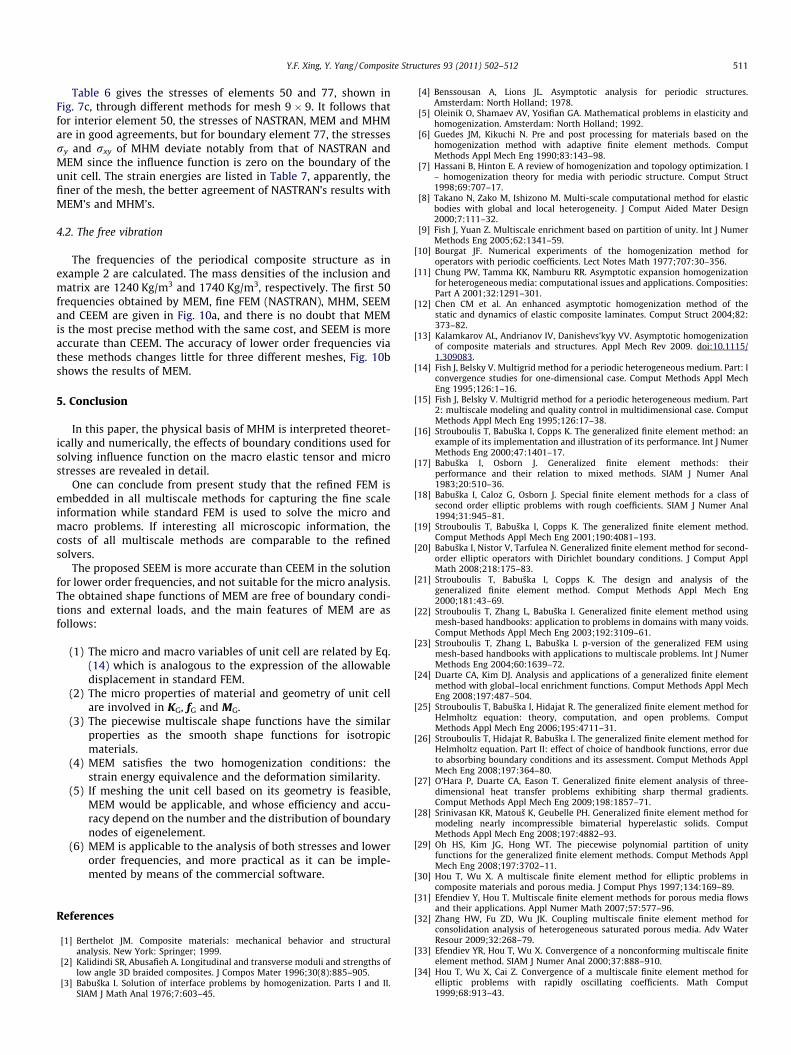
The frequencies of the periodical composite structure as inexample 2 are calculated. The mass densities of the inclusion andmatrix are 1240 Kg/m3 and 1740 Kg/m3, respectively. The first 50frequencies obtained by MEM, fine FEM (NASTRAN), MHM, SEEMand CEEM are given in Fig. 10a, and there is no doubt that MEMis the most precise method with the same cost, and SEEM is moreaccurate than CEEM. The accuracy of lower order frequencies viathese methods changes little for three different meshes, Fig. 10bshows the results of MEM.

5. Conclusion

In this paper, the physical basis of MHM is interpreted theoret-ically and numerically, the effects of boundary conditions used forsolving influence function on the macro elastic tensor and microstresses are revealed in detail.

One can conclude from present study that the refined FEM isembedded in all multiscale methods for capturing the fine scaleinformation while standard FEM is used to solve the micro andmacro problems. If interesting all microscopic information, thecosts of all multiscale methods are comparable to the refinedsolvers.

The proposed SEEM is more accurate than CEEM in the solutionfor lower order frequencies, and not suitable for the micro analysis.The obtained shape functions of MEM are free of boundary condi-tions and external loads, and the main features of MEM are asfollows:

(1) The micro and macro variables of unit cell are related by Eq.(14) which is analogous to the expression of the allowabledisplacement in standard FEM.

(2) The micro properties of material and geometry of unit cellare involved in KG, fG and MG.

(3) The piecewise multiscale shape functions have the similarproperties as the smooth shape functions for isotropicmaterials.

(4) MEM satisfies the two homogenization conditions: thestrain energy equivalence and the deformation similarity.

(5) If meshing the unit cell based on its geometry is feasible,MEM would be applicable, and whose efficiency and accu-racy depend on the number and the distribution of boundarynodes of eigenelement.

(6) MEM is applicable to the analysis of both stresses and lowerorder frequencies, and more practical as it can be imple-mented by means of the commercial software.

References

[1] Berthelot JM. Composite materials: mechanical behavior and structuralanalysis. New York: Springer; 1999.

[2] Kalidindi SR, Abusafieh A. Longitudinal and transverse moduli and strengths oflow angle 3D braided composites. J Compos Mater 1996;30(8):885–905.

[3] Babuška I. Solution of interface problems by homogenization. Parts I and II.SIAM J Math Anal 1976;7:603–45.

[4] Benssousan A, Lions JL. Asymptotic analysis for periodic structures.Amsterdam: North Holland; 1978.

[5] Oleinik O, Shamaev AV, Yosifian GA. Mathematical problems in elasticity andhomogenization. Amsterdam: North Holland; 1992.

[6] Guedes JM, Kikuchi N. Pre and post processing for materials based on thehomogenization method with adaptive finite element methods. ComputMethods Appl Mech Eng 1990;83:143–98.

[7] Hassani B, Hinton E. A review of homogenization and topology optimization. I– homogenization theory for media with periodic structure. Comput Struct1998;69:707–17.

[8] Takano N, Zako M, Ishizono M. Multi-scale computational method for elasticbodies with global and local heterogeneity. J Comput Aided Mater Design2000;7:111–32.

[9] Fish J, Yuan Z. Multiscale enrichment based on partition of unity. Int J NumerMethods Eng 2005;62:1341–59.

[10] Bourgat JF. Numerical experiments of the homogenization method foroperators with periodic coefficients. Lect Notes Math 1977;707:30–356.

[11] Chung PW, Tamma KK, Namburu RR. Asymptotic expansion homogenizationfor heterogeneous media: computational issues and applications. Composities:Part A 2001;32:1291–301.

[12] Chen CM et al. An enhanced asymptotic homogenization method of thestatic and dynamics of elastic composite laminates. Comput Struct 2004;82:373–82.

[13] Kalamkarov AL, Andrianov IV, Danishevs’kyy VV. Asymptotic homogenizationof composite materials and structures. Appl Mech Rev 2009. doi:10.1115/1.309083.

[14] Fish J, Belsky V. Multigrid method for a periodic heterogeneous medium. Part: Iconvergence studies for one-dimensional case. Comput Methods Appl MechEng 1995;126:1–16.

[15] Fish J, Belsky V. Multigrid method for a periodic heterogeneous medium. Part2: multiscale modeling and quality control in multidimensional case. ComputMethods Appl Mech Eng 1995;126:17–38.

[16] Strouboulis T, Babuška I, Copps K. The generalized finite element method: anexample of its implementation and illustration of its performance. Int J NumerMethods Eng 2000;47:1401–17.

[17] Babuška I, Osborn J. Generalized finite element methods: theirperformance and their relation to mixed methods. SIAM J Numer Anal1983;20:510–36.

[18] Babuška I, Caloz G, Osborn J. Special finite element methods for a class ofsecond order elliptic problems with rough coefficients. SIAM J Numer Anal1994;31:945–81.

[19] Strouboulis T, Babuška I, Copps K. The generalized finite element method.Comput Methods Appl Mech Eng 2001;190:4081–193.

[20] Babuška I, Nistor V, Tarfulea N. Generalized finite element method for second-order elliptic operators with Dirichlet boundary conditions. J Comput ApplMath 2008;218:175–83.

[21] Strouboulis T, Babuška I, Copps K. The design and analysis of thegeneralized finite element method. Comput Methods Appl Mech Eng2000;181:43–69.

[22] Strouboulis T, Zhang L, Babuška I. Generalized finite element method usingmesh-based handbooks: application to problems in domains with many voids.Comput Methods Appl Mech Eng 2003;192:3109–61.

[23] Strouboulis T, Zhang L, Babuška I. p-version of the generalized FEM usingmesh-based handbooks with applications to multiscale problems. Int J NumerMethods Eng 2004;60:1639–72.

[24] Duarte CA, Kim DJ. Analysis and applications of a generalized finite elementmethod with global–local enrichment functions. Comput Methods Appl MechEng 2008;197:487–504.

[25] Strouboulis T, Babuška I, Hidajat R. The generalized finite element method forHelmholtz equation: theory, computation, and open problems. ComputMethods Appl Mech Eng 2006;195:4711–31.

[26] Strouboulis T, Hidajat R, Babuška I. The generalized finite element method forHelmholtz equation. Part II: effect of choice of handbook functions, error dueto absorbing boundary conditions and its assessment. Comput Methods ApplMech Eng 2008;197:364–80.

[27] O’Hara P, Duarte CA, Eason T. Generalized finite element analysis of three-dimensional heat transfer problems exhibiting sharp thermal gradients.Comput Methods Appl Mech Eng 2009;198:1857–71.

[28] Srinivasan KR, Matouš K, Geubelle PH. Generalized finite element method formodeling nearly incompressible bimaterial hyperelastic solids. ComputMethods Appl Mech Eng 2008;197:4882–93.

[29] Oh HS, Kim JG, Hong WT. The piecewise polynomial partition of unityfunctions for the generalized finite element methods. Comput Methods ApplMech Eng 2008;197:3702–11.

[30] Hou T, Wu X. A multiscale finite element method for elliptic problems incomposite materials and porous media. J Comput Phys 1997;134:169–89.

[31] Efendiev Y, Hou T. Multiscale finite element methods for porous media flowsand their applications. Appl Numer Math 2007;57:577–96.

[32] Zhang HW, Fu ZD, Wu JK. Coupling multiscale finite element method forconsolidation analysis of heterogeneous saturated porous media. Adv WaterResour 2009;32:268–79.

[33] Efendiev YR, Hou T, Wu X. Convergence of a nonconforming multiscale finiteelement method. SIAM J Numer Anal 2000;37:888–910.

[34] Hou T, Wu X, Cai Z. Convergence of a multiscale finite element method forelliptic problems with rapidly oscillating coefficients. Math Comput1999;68:913–43.

512 Y.F. Xing, Y. Yang / Composite Structures 93 (2011) 502–512

[35] E W, Engquist B. The heterogeneous multiscale methods. Commun Math Sci2003;1:87–132.

[36] E W, Ming PB, Zhang PW. Analysis of the heterogeneous multiscale method forelliptic homogenization problems. J Am Math Soc 2005;18:121–56.

[37] Ming PB, Zhang PW. Analysis of the heterogeneous multiscale method forparabolic homogenization problems. Math Comput 2007;76:153–77.

[38] Ming PB, Yue XY. Numerical methods for multiscale elliptic problems. JComput Phys 2006;214:421–45.

[39] E W, Engquist B. Multiscale modeling and computation. Notice Am Math Soc2003;50:1062–70.

[40] Abdulle A. Heterogeneous multiscale methods with quadrilateral finiteelements. Numer Math Adv Appl 2007;20:743–51.

[41] E W, Engquist B, Li XT, Ren WQ, Vanden-Eijnden E. Heterogeneous multiscalemethods: a review. Commun Comput Phys 2007;2(3):367–450.

[42] E W, Engquist B. The heterogeneous multi-scale method for homogenizationproblems. Lect Notes Comput Sci Eng: Multiscale Methods Sci Eng2006;44:89–110.

[43] Chen ZX. On the heterogeneous multiscale method with various macroscopicsolvers. Nonlinear Anal 2009. doi:10.1016/j.na.2009.01.22.

[44] Xing YF, Yang Y. A new rod eigenelement and its application to structural staticand dynamic analysis. In: Proceedings of international symposium oncomputational mechanics. Beijing, China: Tsinghua University Press andSpringer-Verlag; 2007.

[45] Xing YF, Yang Y, Wang XM. A multiscale eigenelement method and itsapplication to periodical composite structures. Compos Struct2010;92:2265–75.

[46] Berdichevesky VL. On averaging of periodic systems. PMM1977;41(6):993–1006.

[47] Berdichevesky VL. Variational-asymptotic method of constructing a theory ofshells. PMM 1979;43(4):664–86.

[48] Yu W, Tang T. Variational asymptotic method for unit cell homogenization ofperiodically heterogeneous materials. Int J Solids Struct 2007;44(11-12):3738–55.

[49] Xing YF, Tian JM, Zhu DC, Xie WJ. The homogenization method based oneigenvector expansions for woven fabric composites. Int J Multiscale ComputEng 2006;4(1):197–206.

[50] Xing YF, Wang XM. An eigenelement method and two homogenizationconditions. Acta Mech Sin 2009;25(3):345–51.

本文献由“学霸图书馆-文献云下载”收集自网络，仅供学习交流使用。

学霸图书馆（www.xuebalib.com）是一个“整合众多图书馆数据库资源，

提供一站式文献检索和下载服务”的24 小时在线不限IP

图书馆。

图书馆致力于便利、促进学习与科研，提供最强文献下载服务。

图书馆导航：

图书馆首页 文献云下载 图书馆入口 外文数据库大全 疑难文献辅助工具