An Efficient Particle Tracking Algorithm for Large-Scale Parallel Pseudo-SpectralSimulations of Turbulence

Cristian C. Lalescua,b,1, Berenger Bramasc,b,d, Markus Ramppb, Michael Wilczeka

aMax Planck Institute for Dynamics and Self-Organization, Goettingen, GermanybMax Planck Computing and Data Facility, Garching, Germany

cInria Nancy – Grand-Est, CAMUS Team, FrancedICube, ICPS Team, France

Abstract

Particle tracking in large-scale numerical simulations of turbulent flows presents one of the major bottlenecks in parallel perfor-mance and scaling efficiency. Here, we describe a particle tracking algorithm for large-scale parallel pseudo-spectral simulations ofturbulence which scales well up to billions of tracer particles on modern high-performance computing architectures. We summarizethe standard parallel methods used to solve the fluid equations in our hybrid MPI/OpenMP implementation. As the main focus,we describe the implementation of the particle tracking algorithm and document its computational performance. To address theextensive inter-process communication required by particle tracking, we introduce a task-based approach to overlap point-to-pointcommunications with computations, thereby enabling improved resource utilization. We characterize the computational cost as afunction of the number of particles tracked and compare it with the flow field computation, showing that the cost of particle trackingis very small for typical applications.

Keywords: Particle tracking; MPI; OpenMP

1. Introduction

Understanding particle transport in turbulent flows is funda-mental to the problem of turbulent mixing [1, 2, 3, 4, 5, 6]and relevant for a wide range of applications such as disper-sion of particles in the environment [7, 8, 9, 10], the growthof cloud droplets through collisions [11, 12, 13, 14, 15], andphytoplankton swimming in the ocean [16, 17, 18]. Direct nu-merical simulations (DNS) of turbulence are nowadays an es-tablished tool for investigating such phenomena and have a longhistory in scientific computing [19, 20, 21, 22, 23]. DNS havebecome a major application and technology driver in high per-formance computing, since the scale separation between thelargest and the smallest scales increases drastically with theReynolds number Rλ, which characterizes the degree of small-scale turbulence [24]. Dimensional estimates of the requiredcomputational resources scale at least as R6

λ [24]. Recent lit-erature [25], however, shows that, due the occurrence of ex-tremely small-scale structures, resolution requirements increaseeven faster than simple dimensional arguments suggest. Untiltoday DNS have reached values of up to Rλ ≈ 2300 [26, 27, 22],still smaller than the latest experiments, which have reachedRλ > 5000 [28], or natural settings such as cumulus clouds,which show Reynolds numbers on the order of 104 [29]. HenceDNS of turbulence will continue to be computationally de-manding for the foreseeable future.

∗Corresponding author.E-mail address: Cristian.Lalescu@mpcdf.mpg.de

Due to the large grid sizes, practical implementations ofDNS typically employ one- or two-dimensional domain de-compositions within a distributed memory parallel program-ming paradigm. While the numerical solution of the fieldequations is typically achieved with well-established methods,the efficient implementation of particle tracking within suchparallel approaches still poses major algorithmic challenges.In particular, particle tracking requires an accurate interpola-tion of the flow fields on distributed domains and particlestraversing the domain need to be passed on from one sub-domain/process to another. As the Reynolds number increases,the number of particles required to adequately sample the tur-bulent fields needs to grow with the increasing numerical res-olution, since this is a measure of the degrees of freedom ofthe flow. In addition higher-order statistics might be neededto address specific research questions, and thus the numberof particles required for converged statistics increases as well[4, 30, 31, 32, 33, 34, 35, 36]. Overall, this requires an ap-proach which handles the parallel implementation in an effi-cient manner for arbitrarily accurate methods. One option ex-plored in the literature is the use of the high-level program-ming concept of coarrays, in practice shifting responsibilityfor some of the communication operations to the compiler, see[23]. The general solution that we describe makes use of MPIand OpenMP for explicit management of hardware resources.The combination of MPI [37] and OpenMP [38] has become ade facto standard in the development of large-scale applications[39, 40, 41, 42, 43, 44]. MPI [45] is used for communicationbetween processes and OpenMP to manage multiple execution

Preprint submitted to Computer Physics Communications July 5, 2021

arX

iv:2

107.

0110

4v1

[ph

ysic

s.fl

u-dy

n] 2

Jul

202

1

threads over multicore CPUs using shared memory. Separately,large datasets must be processed with specific data-access pat-terns to make optimal use of modern hardware, as explained forexample in [46].

To address the challenges outlined above, we have developedthe numerical framework “Turbulence Tools: Lagrangian andEulerian” (TurTLE), a flexible pseudo-spectral solver for fluidand turbulence problems implemented in C++ with a hybridMPI/OpenMP approach [47]. TurTLE allows for an efficienttracking of a large class of particles. In particular, TurTLEshowcases a parallel programming pattern for particle track-ing that is easy to adapt and implement, and which allows ef-ficient executions at both small and large problem sizes. Ourevent-driven approach is especially suited for the case whereindividual processes require data exchanges with several otherprocesses while also being responsible for local work. For this,asynchronous inter-process communication and tasks are used,based on a combined MPI/OpenMP implementation. As wewill show in the following, TurTLE permits numerical parti-cle tracking at relatively small costs, while retaining flexibilitywith respect to number of particles and numerical accuracy. Weshow that TurTLE scales well up to O(104) computing cores,with the flow field solver approximately retaining the perfor-mance of the used Fourier transform libraries for DNS with3 × 20483 and 3 × 40963 degrees of freedom. We also mea-sure the relative cost of tracking up to 2.2 × 109 particles asapproximately only 10% of the total wall-time for the 40963

case, demonstrating the efficiency of the new algorithm evenfor very demanding particle-based studies.

In the following, we introduce TurTLE and particularly fo-cus on the efficient implementation of particle tracking. Sec-tion 2 introduces the evolution equations for the fluid and par-ticle models, as well as the corresponding numerical methods.Section 3 provides an overview of our implementation, includ-ing a more detailed presentation of the parallel programmingpattern used for particle tracking. Finally, Section 4 summa-rizes a performance evaluation using up to 512 computationalnodes.

2. Evolution equations and numerical method

2.1. Fluid equations

While TurTLE is developed as a general framework for alarger class of fluid equations, we focus on the Navier-Stokesequations as prototypical example in the following. The incom-pressible Navier-Stokes equations take the form

∂tu + u · ∇u = −∇p + ν∆u + f ,∇ · u = 0.

(1)

Here, u denotes the three-dimensional velocity field, p is thekinematic pressure, ν is the kinematic viscosity, and F denotesan external forcing that drives the flow. We consider periodicboundary conditions, which allows for the use of a Fourierpseudo-spectral scheme. Within this scheme, a finite Fourierrepresentation is used for the fields, and the non-linear term

of the Navier-Stokes equations is computed in real space —an approach pioneered by Orszag and Patterson [19]. For theconcrete implementation in TurTLE, we use the vorticity for-mulation of the Navier-Stokes equation, which takes the form

∂tω(x, t) = ∇ × (u(x, t) × ω(x, t)) + ν∆ω(x, t) + F(x, t), (2)

where ω = ∇×u is the vorticity field and F = ∇× f denotes thecurl of the Navier-Stokes forcing. The Fourier representation ofthis equation takes the form [48, 49]

∂tω(k, t) = ik×F [u(x, t)×ω(x, t)]− νk2ω(k, t) + F(k, t), (3)

where F is the direct Fourier transform operator. In Fourierspace, the velocity can be conveniently computed from the vor-ticity using Biot-Savart’s law,

u(k, t) =ik × ω(k, t)

k2 . (4)

Equation (3) is integrated with a third-order Runge-Kuttamethod [50], which is an explicit Runge-Kutta method with theButcher tableau (5)

01 1

1/2 1/4 1/41/6 1/6 2/3

(5)

In addition to the stability properties described in [50], thismethod has the advantage that it is memory-efficient, requir-ing only two additional field allocations, as can be seen from

w1(k) = ω(k, t)e−νk2h + hN[ω(k, t)]e−νk

2h,

w2(k) = 34 ω(k, t)e−νk

2h/2 + 14 (w1(k) + hN[w1(k)])eνk

2h/2,

ω(k, t + h) = 13 ω(k, t)e−νk

2h + 23 (w2(k) + hN[w2(k)])e−νk

2h/2,(6)

where h is the time step, limited in practice by theCourant–Friedrichs–Lewy (CFL) condition [51]. The nonlin-ear term

N[w(k)] = ik × F[F −1

[ik×w(k)

k2

]× F −1 [w(k)]

](7)

is computed by switching between Fourier space and real space.If the forcing term is nonlinear, it can be included in the right-hand side of (7). To treat the diffusion term, we use the standardintegrating factor technique [52] in (6).

Equation (3) contains the Fourier transform of a quadraticnonlinearity. Since numerical simulations are based on finiteFourier representations, the real-space product of the two fieldswill in general contain unresolved high-frequency harmonics,leading to aliasing effects [52]. In TurTLE, de-aliasing isachieved through the use of a smooth Fourier filter, an approachthat has been shown in [53] to lead to good convergence to thetrue solution of a PDE, even though it does not completely re-move aliasing effects.

2

The Fourier transforms in TurTLE are evaluated using theFFTW library [54]. Within the implementation of the pseudo-spectral scheme, the fields have two equivalent representations:an array of Fourier mode amplitudes, or an array of vectorialvalues on the real-space grid. For the simple case of 3D pe-riodic cubic domains of size [0, 2π]3, the real space grid is arectangular grid of N × N × N points, equally spaced at dis-tances of δ ≡ 2π/N. Exploiting the Hermitian symmetry ofreal fields, the Fourier-space grid consists of N × N × (N/2 + 1)modes. Therefore, the field data consists of arrays of floatingpoint numbers, logically shaped as the real-space grid or arraysof floating point number pairs (e.g. fftw complex) logicallyshaped as the Fourier-space grid. Extensions to non-cubic do-mains or non-isotropic grids are straightforward.

The direct numerical simulation algorithm then has two fun-damental constructions: loops traversing the fields, with an as-sociated cost of O(N3) operations, and direct/inverse Fouriertransforms, with a cost of O(N3 log N) operations.

2.2. Particle equations

A major feature of TurTLE is the capability to track differentparticle types, including Lagrangian tracer particles, ellipsoids,self-propelled particles and inertial particles. To illustrate theimplementation, we focus on tracer particles in the following.

Lagrangian tracer particles are virtual markers of the flowfield starting from the initial position x. Their position Xevolves according to

ddt X(x, t) = u(X(x, t), t), X(x, 0) = x. (8)

The essential characteristic of such particle equations is thatthey require as input the values of various flow fields at arbitrarypositions in space.

TurTLE combines multi-step Adams-Bashforth integrationschemes (see, e.g., §6.7 in [55]) with a class of spline inter-polations [56] in order to integrate the ODEs. Simple Lagrangeinterpolation schemes (see, e.g., §3.1 in [55]) are also imple-mented in TurTLE for testing purposes. There is ample litera-ture on interpolation method accuracy, efficiency, and adequacyfor particle tracking, e.g. [20, 57, 58, 59, 60]. The common fea-ture of all interpolation schemes is that they can be representedas a weighted real-space-grid average of a field, with weightsgiven by the particle’s position. For all practical interpolationschemes, the weights are zero outside of a relatively small ker-nel of grid points surrounding the particle, i.e. the formulas are“local”. For some spline interpolations, a non-local expressionis used, but it can be rewritten as a local expression where thevalues on the grid are precomputed through a distinct globaloperation [20] — this approach, for example, is used in [23].

Thus an interpolation algorithm can be summed up as fol-lows:

1. compute X = X mod 2π (because the domain is peri-odic).

2. find the closest grid cell to the particle position X, indexedby c ≡ (c1, c2, c3).

3. compute x = X − cδ.

4. compute a sum of the field over I grid points in each of the3 directions, weighted by some polynomials:

u(X) ≈I/2∑

i1,i2,i3=1−I/2

βi1

(x1δ

)βi2

(x2δ

)βi3

(x3δ

)u(c + i). (9)

The cost of the sum itself grows as I3, the cube of the size of theinterpolation kernel. The polynomials βi j are determined by theinterpolation scheme (see [56]).

In general accuracy improves with increasing I. In TurTLE,interpolation is efficiently implemented even at large I. As dis-cussed below in §3.3, this is achieved by organizing particledata such that only O(I2) MPI messages are required to com-plete the triple sum, rather than O(Np).

3. Implementation

3.1. OverviewThe solver relies on two types of objects. Firstly, an ab-

stract class encapsulates three elements: generic initialization,do work and finalization functionality. Secondly, essential datastructures (i.e. fields, sets of particles) and associated function-ality (e.g. HDF5-based I/O) are provided by “building block”-classes. The solver then consists of a specific “arrangement” ofthe building blocks.

The parallelization of TurTLE is based on a standard, MPI-based, one-dimensional domain-decomposition approach: Thethree-dimensional fields are decomposed along one of the di-mensions into a number of slabs, with each MPI process hold-ing one such slab. In order to efficiently perform the costlyFFT operations with the help of a high-performance numeri-cal library such as FFTW, process-local, two-dimensional FFTsare interleaved with a global transposition of the data in orderto perform the FFTs along the remaining dimension. A well-known drawback of the slab decomposition strategy offered byFFTW is its limited parallel scalability, because at most N MPIprocesses can be used for N3 data. We compensate for this byutilizing the hybrid MPI/OpenMP capability of FFTW (or func-tionally equivalent libraries such as Intel MKL), which allowsto push the limits of scalability by at least an order of magni-tude, corresponding to the number of cores of a modern multi-core CPU or NUMA domain, respectively. All other relevantoperations in the field solver can be straightforwardly paral-lelized with the help of OpenMP. Our newly developed parallelparticle tracking algorithm has been implemented on top of thisslab-type data decomposition using MPI and OpenMP, as shallbe detailed below. Slab decompositions are beneficial for parti-cle tracking since MPI communication overhead is minimizedcompared to, e.g., two-dimensional decompositions.

3.2. Fluid solverThe fluid solver consists of operations with field data, which

TurTLE distributes among a total of P MPI processes with astandard slab decomposition, see Fig. 1. Thus the logical field

3

Process #0 ... ... ... ... ... Process #P 1x3{Ps slices

Pp particles

Sp particles

...

Sp particles

...

Sp particles

Figure 1: Distribution of real-space data between MPI processes in TurTLE.Fields are split into slabs and distributed between P MPI processes along the x3direction. The Np particles are also distributed, with each MPI process storingPp particles on average. Within each MPI process the particle data is sortedaccording to its x3 location. This leads to a direct association between each ofthe Ps field slices to contiguous regions of the particle data arrays — in turnsimplifying the interpolation procedure (see text for details). On average, S pparticles are held within each such contiguous region.

layouts consist of (N/P)×N×N points for the real-space repre-sentation, and (N/P)×N×(N/2+1) points for the Fourier spacerepresentation. This allows the use of FFTW [54] to performcostly FFT operations, as outlined above. We use the conven-tion that fields are distributed along the real-space x3 direction,and along the k2 direction in the Fourier space representation(directions 2 and 3 are transposed between the two represen-tations). Consequently, a problem on an N3 grid can be par-allelized on a maximum of N computational nodes using oneMPI process per node and, possibly, OpenMP threads insidethe nodes, see Fig. 1.

In the interest of simplifying code development, TurTLEuses functional programming for the costly traversal operation.Functional programming techniques allow to encapsulate fielddata in objects, while providing methods for traversing the dataand computing specified arithmetic expressions — i.e. the classbecomes a building block. While C++ allows for overloadingarithmetic operators as a mechanism for generalizing them toarrays, our approach permits to combine several operations ina single data traversal, and it applies directly to operations be-tween arrays of different shapes. In particular operations suchas the combination of taking the curl and the Laplacian of a field(see (3)) are in practice implemented as a single field traversaloperation.

3.3. Particle tracking

We now turn to a major feature of TurTLE: the efficient track-ing of particles. The novelty of our approach warrants a morein-depth presentation of the data structure and the parallel al-gorithms, for which we introduce the following notations (seealso Fig. 1):

• P : the number of MPI processes (should be a divisor ofthe field grid size N);

• Ps = N/P : the number of field slices in each slab;

• Np : the number of particles in the system;

• Pp: the number of particles contained in a given slab (i.e.hosted by the corresponding process) — on average equalto Np/P;

• S p: the number of particles per slice, i.e. number of par-ticles found between two slices — on average equal toNp/N;

• I : the width of the interpolation kernel, i.e. the number ofslices needed to perform the interpolation.

The triple sum (9) is effectively split into I double sums overthe x1 and x2 directions, the results of which then need to be dis-tributed/gathered among the MPI processes such that the sumalong the x3 direction can be finalized. Independently of P andN, there will be Np sums of I3 terms that have to be performed.However, the amount of information to exchange depends onthe DNS parameters N, Np, and I, and on the job parameter P.

Whenever more than one MPI process is used, i.e. P > 1, wedistinguish between two cases:

1. I ≤ Ps, i.e. each MPI domain extends over at least as manyslices as required for the interpolation kernel. In this caseparticles are shared between at most two MPI processes,therefore each process needs to exchange information withtwo other processes. In this case, the average number ofshared particles is S p(I − 2).

2. I > Ps, i.e. the interpolation kernel always extends outsideof the local MPI domain. The average number of sharedparticles is S pPs. Each given particle is shared amonga maximum of dI/Pse processes, therefore each processmust in principle communicate with 2dI/Pse−1 other pro-cesses.

The second scenario is the more relevant for scaling studies.Our expectation is that the communication costs will outweighthe computation costs, therefore the interpolation step shouldscale like NpI/Ps ∝ NpIP/N. In the worst case scenario, whenthe 2D sum has a significant cost as well, we expect scaling likeNpI3P/N.

3.3.1. Particle data structureThe field grid is partitioned in one dimension over the pro-

cesses, as described in Section 3.2, such that each process ownsa field slab. For each process, we use two arrays to store the datafor particles included inside the corresponding slab. The first ar-ray contains state information, including the particle locations— required to perform the interpolation of the field. The sec-ond array, called rhs, contains the value of the right-hand-sideof (8), as computed at the most recent few iterations (as re-quired for the Adams-Bashforth integration); updating this sec-ond array requires interpolation. The two arrays use an arrayof structures pattern, in the sense that data associated to oneparticle is contiguous in memory. While this may lead to per-formance penalties, as pointed out in [46], there are significant

4

benefits for our MPI parallel approach, as explained below. Wesummarize in the following the main operations that are appliedto the arrays.

Ordering the particles locally. When N > P, processes are incharge of more than one field slice, and the particles in theslab are distributed across different slices. In this case, westore the particles that belong to the same slice contiguously inthe arrays, one slice after the other in increasing x3-axis order.This can be achieved by partitioning the arrays into Ps differ-ent groups and can be implemented as an incomplete Quicksortwith a complexity of O(Pp log Ps) on average. After this oper-ation, we build an array offset of size Ps + 1, where offset[idx]returns the starting index of the first particle for the partition idxand offset[idx+1]-offset[idx] the number of particles in groupidx. As a result, we have offset[Ps]= Pp. This allows direct ac-cess to the contiguous data regions corresponding to each fieldslice, in turn relevant for MPI exchanges (see below).

Exchanging the particles for computation. With our data struc-tures, we are able to send the state information of all the par-ticles located in a single group with only one communication,which reduces communication overhead. Moreover, sendingthe particles from several contiguous levels can also be donein a single operation because the groups are stored sequentiallyinside the arrays.

Particles displacement/update. The positions of the particlesare updated at the end of each iteration, and so the arrays mustbe rearranged accordingly. The changes in the x3 directionmight move some particles in a different slice and even on aslice owned by a different process. Therefore, we first partitionthe first and last groups (the groups of the first and last slicesof the process’s slab) to move the particles that are now outsideof the process’s grid interval at the extremities of the arrays.We only act on the particles located at the lower and highergroups because we assume that the particles cannot move withdistance greater than 2π/N. For regular tracers (8) this is in factrequired by the CFL stability condition of the fluid solver. Thispartitioning is done with a complexity O(Pp/Ps). Then, everyprocess exchanges those particles with its direct neighbors, en-suring that the particles are correctly distributed. Finally, eachprocess sorts its particles to take into account the changes in thepositions and the newly received particles as described previ-ously.

3.3.2. ParallelizationThe interpolation of the field at the particle locations concen-

trates most of the workload of the numerical particle tracking.For each particle, the interpolation uses the I3 surrounding fieldnodes. However, because we do not mirror the particle or thefield information on multiple processes, we must actively ex-change either field or particle information to perform a com-plete interpolation. Assuming that the number of particles inthe simulation is much less than the number of field nodes, i.e.the relation Pp < IN2 holds, less data needs to be transferred onaverage when particle locations are exchanged rather than field

T3T2T1T0

Post initial sends/receives

Send completed, nothing to do, wait again

Other’s data received

Insert task for computation on received data

Post the send for the result

Other’s data received

Insert task for computation on received data

Post the send for the result

Result related to local data received, do nothing

Merge

Wait any communication to be completed

Wait any communication to be completed

Wait any communication to be completed

Wait any communication to be completed

Idle

Insert task for computation on local data

Compute a task on local data

Compute a task on received data

Wait two last send to be done

All communication completedEnd of parallel section

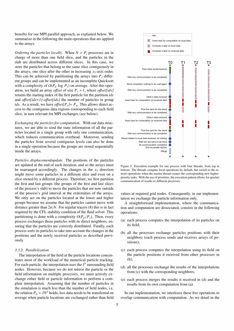
Figure 2: Execution example for one process with four threads, from top tobottom. The threads compute local operations by default, but switch to the re-mote operations when the master thread creates the corresponding new higher-priority tasks. With the use of priorities, the execution pattern allows for quickercommunication of results to different processes.

values at required grid nodes. Consequently, in our implemen-tation we exchange the particle information only.

A straightforward implementation, where the communica-tion and computation are dissociated, consists in the followingoperations:

(a) each process computes the interpolation of its particles onits field;

(b) all the processes exchange particles positions with theirneighbors (each process sends and receives arrays of po-sitions);

(c) each process computes the interpolation using its field onthe particle positions it received from other processes in(b);

(d) all the processes exchange the results of the interpolationsfrom (c) with the corresponding neighbors;

(e) each process merges the results it received in (d) and theresults from its own computation from (a).

In our implementation, we interleave these five operations tooverlap communication with computation. As we detail in the

5

following, the master thread of each MPI process creates com-putation work packages, then performs communications whilethe other threads are already busy with the work packages. Thisis achieved with the use of non-blocking MPI communicationsand OpenMP tasks, as illustrated in Fig. 2. In a first stage, themaster thread splits the local interpolation from (a) into tasksand submits them immediately but with a low priority. Then, itposts all the sends/receives related to (b) and all the receives re-lated to (d), and stores the corresponding MPI requests in a listR. In the core part of the algorithm, the master thread performsa wait-any on R. This MPI function is blocking and returnsas soon as one of the communications in the list is completed.Hence, when a communication is completed, the master threadacts accordingly to the type of event e it represents. If e is thecompletion of a send of local particle positions, from (b), thereis nothing to do and the master thread directly goes back to thewait-any on R. In this case, it means that a send is completedand that there is nothing new to do locally. If e is the com-pletion of a receive of remote particle positions, from (b), thenthe master thread creates tasks to perform the interpolation ofthese positions, from (c), and submits them with high priority.Setting a high priority ensures that all the threads will work onthese tasks even if the tasks inserted earlier to interpolate thelocal positions, from (a), are not completed. When these tasksare completed, the master thread posts a non-blocking send tocommunicate the results to the process that owns the particlesand stores the corresponding MPI request in R. Then, the mas-ter thread goes back to the wait-any on R. If e is the com-pletion of a send of interpolation on received positions, as justdescribed, the master thread has nothing to do and goes back tothe wait-any. In fact, this event simply means that the resultswere correctly sent. If e is the completion of a receive, from(d), of interpolation performed by another process, done in (c),the master thread keeps the buffer for merging at the end, and itgoes back to the wait-any on R. When R is empty, it means thatall communications (b,d) but also computations on other posi-tions (c) are done. If some local work still remains from (a),the master thread can join it and compute some tasks. Finally,when all computation and communication are over, the threadscan merge the interpolation results, operation (e).

The described strategy is a parallel programming pattern thatcould be applied in many other contexts when there are localand remote works to perform and where remote work meansfirst to exchange information and second to apply computationon it.

3.4. In-Order Parallel Particle I/O

Saving the states of the particles on disk is a crucial operationto support checkpoint/restart and for post-processing. We focuson output because TurTLE typically performs many more out-put than input operations (the latter only happen during initial-ization). The order in which the particles are saved is importantbecause it influences the writing pattern and the data accessesduring later post-processing of the files. As the particles moveacross the processes during the simulation, a naive output of theparticles as they are distributed will lead to inconsistency from

11 3 7 5 10 6 12 2 4 0 13 8 9 1 14

3 5 7 11 6 10 12 0 2 4 8 9 13 1 14

3 5 7 11 6 10 12 0 2 4 8 9 13 1 14

3 5 7 6 0 2 4 11 10 12 8 9 13 14

0 1 2 3 4 5 6 8 9 10 11 12 13 14

1

7

P0 P1 P2 P3

P0 P1 P2 P3

P0 P1 P2 P3

Sort

Split

Send/Recv

Sort

P0 P1

P0 P1

0 1 2 3 4 5 6 8 9 10 11 12 13 147

Write to file

Figure 3: The different stages to perform a parallel saving of the particles inorder. Here, we consider that the particle data (illustrated by the global particleindex) is distributed among 4 processes, but that only 2 of them are used in thewrite operation.

one output to the other. Such a structure would require reorder-ing the particles during the post-processing or would result incomplex file accesses. That is why we save the particles in or-der, i.e. in the original order given as input to the application.

The algorithm that we use to perform the write operationis shown in Fig. 3. There are four main steps to the proce-dure: pre-sort (”Sort” and ”Split” in the figure), followed byexchange (”Send/Recv” in Fig. 3), with a final post-sort beforethe actual HDF5 write.

Each process first sorts its local particles using the globalindices, which is done with a O(Pp log Pp) complexity. Thissort can be done in parallel using multiple threads. Then, eachprocess counts the number of particles it has to send to eachof the processes that are involved in the file writing. Thesenumbers are exchanged between the processes allowing eachprocess to allocate the reception buffer. If we consider that PO

processes are involved in the output operation, each of themshould receive Np/PO particles in total, and a process of rank rshould receive the particles from index r × Np/PO to (r + 1) ×Np/PO − 1.

In the exchange step, the particles can be sent either withmultiple non-blocking send/receive or with a single all-to-alloperation, with the total number of communications boundedby P × PO. Finally, the received particles are sorted with acomplexity of O(Np/PO log Np/PO), and written in order intothe output file.

The number PO of processes involved in the writing shouldbe carefully chosen because as PO increases, the amount ofdata output per process decreases and might become so smallthat the write operation becomes inefficient. At the same time,the preceding exchange stage becomes more and more simi-lar to a complete all-to-all communication with N2

p relatively

6

32 64 128 256 512Number of nodes

101

Exec

utio

n tim

e [s

]

a Execution times on SuperMUC-NG

N = 2048, 16 ppnN = 2048, 8 ppnN = 4096, 8 ppn

128 256 512Number of nodes

0

5

10

15

20

25

30

35

40

Exec

utio

n tim

e[s]

b N = 4096, 8 ppn, Np = 108

PDE_FFTPDE_miscIFT for PTPT

Figure 4: Computational performance of TurTLE. Strong scaling behavior of the total runtime (a) for grid size of N = 2048 and N = 4096, respectively, and using8 or 16 MPI processes per node (ppn) on up to 512 fully populated nodes (24576 cores) of SuperMUC-NG (I = 8, Np = 108). For N = 4096 and 8 ppn panel(b) shows a breakdown of the total runtime into the main algorithmic parts, namely solving the system of Navier Stokes partial differential equations (”PDE misc”and ”PDE FFT”) which is largely dominated by the fast Fourier transforms (”PDE FFT”). The cost of particle tracking for 108 particles (with I = 8) is determinedby an additional inverse Fourier transform (”IFT for PT”), whereas the runtime for our novel particle tracking algorithm (”PT”) is still negligible for 108 particles.Hatched regions represent the fraction of MPI communication times.

small messages. On the other hand, as PO decreases, the size ofthe messages exchanged will increase, and the write operationcan eventually become too expensive for only a few processes,which could also run out of memory. This is why we heuris-tically fix PO using three parameters: the minimum amount ofdata a process should write, the maximum number of processesinvolved in the write operation, and a chunk size. As Np in-creases, PO increases up to the given maximum. If Np is largeenough, the code simply ensures that PO − 1 processes outputthe same amount of data (being a multiple of the chunk size),and the last process writes the remaining data. In our imple-mentation, the parameters are chosen empirically (based on ourexperience with several HPC clusters running the IBM GPF-S/SpectrumScale parallel file system), and they can be tunedfor specific hardware configurations if necessary.

We use a similar procedure for reading the particle state: PO

processes read the data, they sort it according to spatial location,then they redistribute it to all MPI processes accordingly.

4. Computational performance

4.1. Hardware and software environmentTo evaluate the computational performance of our ap-

proach, we perform benchmark simulations on the HPC clus-ter SuperMUC-NG from the Leibniz Supercomputing Centre(LRZ): we use up to 512 nodes containing two Intel Xeon Plat-inum 8174 (Skylake) processors with 24 cores each and a baseclock frequency of 3.1 GHz, providing 96 GB of main mem-ory. The network interconnect is an Intel OmniPath (100 Gbit/s)with a pruned fat-tree topology that enables non-blocking com-munications within islands of up to 788 nodes. We use the In-tel compiler 19.0, Intel MPI 2019.4, HDF5 1.8.21 and FFTW3.3.8. For our benchmarks, we always fully populate thenodes, i.e. the combination of MPI processes per node (ppn)

and OpenMP threads per MPI process is chosen such that theirproduct equals 48, and that the threads spawned by an MPI rankare confined within the NUMA domain defined by a single pro-cessor.

4.2. Overall performance

Figure 4 provides an overview of the overall parallel scalingbehavior of the code for a few typical large-scale setups (panela) together with a breakdown into the main algorithmic steps(panel b). We use the execution time for a single time step (av-eraged over a few steps) as the primary performance metric andall data and computations are handled in double precision. Theleft panel shows, for two different setups (N = 2048, 4096),that the code exhibits excellent strong-scaling efficiency (thedashed line represents ideal scaling) from the minimum num-ber of nodes required to fit the code into memory up to the upperlimit which is given by the maximum number of MPI processesthat can be utilized with our one-dimensional domain decom-position. Comparing the blue and the orange curve, i.e. thesame problem computed with a different combination MPI pro-cesses per node (8, 16) and a corresponding number of OpenMPthreads per process (6, 3), a good OpenMP efficiency (which ismostly determined by the properties of the FFT library used,see below) can be noted for the case of 64 nodes. While thebreakdown of OpenMP efficiency from 3 (blue dot) to 6 (or-ange dot) at 128 nodes is likely caused by a peculiarity of theMPI/OpenMP implementation of the FFTW library (see the dis-cussion below), we find that the OpenMP efficiency of FFTW(and hence TurTLE) in general is currently limited to a maxi-mum of 6 to 8 threads per MPI process for the problem sizesconsidered here.

For the example of the large setup (N = 4096) with 8 pro-cesses per node and using 512 nodes (corresponding to the

7

128 256 512Number of nodes

103

102

101

100

Elap

sed

time

[s]

a PT execution times on SuperMUC-NG

I = 4, Np = 106

I = 6, Np = 106

I = 8, Np = 106

I = 4, Np = 108

I = 6, Np = 108

I = 8, Np = 108

I = 4, Np = 2.2×109

I = 6, Np = 2.2×109

I = 8, Np = 2.2×109

128 256 512Number of nodes

0.00

0.05

0.10

0.15

Elap

sed

time

[s]

64%55% 65%

68%

59%64%

61%

54%

67%

b

redistributeinterpolate

106 108 2.2×109Number of particles

0.00

0.25

0.50

0.75

1.00

Frac

tion

of e

laps

ed ti

me 75% 65% 78%75% 64% 75%72% 67% 58%c

Np

= 10

8

I = 4 I = 6 I = 8 I = 4 I = 6 I = 8 I = 4 I = 6 I = 8

512

node

s

Figure 5: Computational performance of the particle tracking code using 8 MPI processes per node and a DNS of size N = 4096, for different sizes of theinterpolation kernel I. Panel (a): strong scaling for different numbers of particles Np and sizes of the interpolation kernel (memory requirements limit the Np =

2.2 × 109 case to 512 nodes). The dashed line corresponds to ideal strong scaling. Panel (b): contributions of interpolation and redistribution operations to the totalexecution time, for a fixed number of particles, Np = 108, and for different sizes of the interpolation kernel (the corresponding vertical bars are distinguished byhatch style, see labels on top) as a function of the number of compute nodes. Panel (c): relative contributions of interpolation and redistribution as a function of Np.Percentages represent the fraction of time spent in MPI calls.

rightmost green dot in the left panel), Fig. 4b shows that the to-tal runtime is largely dominated by the fast Fourier transformsfor solving the system of Navier Stokes partial differential equa-tions (labeled ”PDE FFT”, entire blue area). With increasingnode count, the latter in turn gets increasingly dominated by anall-to-all type of MPI communication pattern which is arisingfrom the global transpositions (blue-hatched area) of the slab-decomposed data. The plot also shows that the deviation fromideal scaling at 256 nodes that is apparent from the left panel iscaused by a lack of scaling of the process-local (i.e. non MPI)operations of the FFTs (blue, non-hatched area). Our analysissuggests that this is caused by a particular OpenMP inefficiencyof FFTW which occurs for certain dimensions of the local dataslabs: In the case of 256 nodes, FFTW cannot efficiently usemore than 3 OpenMP threads for parallelizing over the localslabs of dimension 2 × 4096 × 2049, whereas good scaling upto the desired maximum of 6 threads is observed for a dimen-sion of 8 × 4096 × 2049 (128 nodes) and also 1 × 4096 × 2049(512 nodes). The same arguments applies for the smaller setup(N = 2048) on 128 nodes. We plan for TurTLE to support FFTsalso from the Intel Math Kernel Library (MKL) which are ex-pected to deliver improved threading efficiency.

For practical applications, a user needs to perform a fewexploratory benchmarks for a given setup of the DNS on theparticular computational platform, and available node countsin order to find an optimal combination of MPI processesand OpenMP threads. Since the runtime per timestep is con-stant for our implementation of the Navier-Stokes solver, a fewtimesteps are sufficient for tuning a long-running DNS.

Thanks to our efficient and highly scalable implementationof the particle tracking, its contribution to the total runtime is

barely noticeable in the figure (”PT”, purple colour in Fig. 4b).This holds even for significantly larger numbers of particlesthan the value of Np = 108 which was used here (see belowfor an in-depth analysis). The only noticeable additional costfor particle tracking, amounting to roughly 10% of the totalruntime, comes from an additional inverse FFT (”IFT for PT”,green colour) which is required to compute the advecting vectorfield, which is independent of Np and scales very well.

Finally, Fig. 4a also suggests good weak scaling behavior ofTurTLE: When increasing the problem size from N = 2048 toN = 4096 and at the same time increasing the number of nodesfrom 64 to 512, the runtime increases from 10.35s to 11.45s,which is consistent with a O(N3 log N) scaling of the runtime,given the dominance of the FFTs.

4.3. Particle tracking performanceFig. 5 provides an overview and some details of the perfor-

mance of our particle tracking algorithm, extending the assess-ment of the previous subsection to particle numbers beyond thecurrent state of the art [23]. We use the same setup of a DNSwith N = 4096 and 8 MPI processes per node on SuperMUC-NG, as presented in the previous subsection.

Fig. 5a summarizes the strong-scaling behavior on 128, 256or 512 nodes of SuperMUC-NG for different numbers of parti-cles (106, 108 and 2.2 × 109) and for different sizes of the inter-polation kernel I (4, 6, 8). Most importantly, the absolute runtimes are small compared to the fluid solver: Even when usingthe most accurate interpolation kernel, a number of 2.2 × 109

particles can be handled within less than a second (per timestep), i.e. less than 10% to the total computational cost of Tur-TLE on 512 nodes per time step (cf. Fig. 4).

8

The case of Np = 106 is shown only for reference here. Thisnumber of particles is too small to expect good scalability inthe regime of 128 compute nodes and more. Still, the absoluteruntimes are minuscule compared to a DNS of typical size. ForNp = 108 we observe good but not perfect strong scaling, inparticular for the largest interpolation kernel (I = 8), suggestingthat we observe the NpIP/N regime, as discussed previously. Itis worth mentioning that we observe a sub-linear scaling of thetotal runtime with the total number of particles (Fig. 5a).

Fig. 5b shows a breakdown of the total runtime of the particletracking algorithm into its main parts, interpolation (operationsdetailed in Fig. 2, shown in orange) and redistribution (localsorting of particles together with particle exchange, blue), to-gether with the percentage of time spent in MPI calls. The lat-ter takes between half and two thirds of the total runtime forNp = 108 particles (cf. upper panel b) and reaches almost 80%for Np = 2.2×109 particles on 512 nodes (lower panel c). Over-all, the interpolation cost always dominates over redistribution,and increases with the size of the interpolation kernel roughlyas I2, i.e. the interpolation cost is proportional to the number ofMPI messages required by the algorithm (as detailed above).

4.4. Particle output

128 256 512Number of nodes

0

1

2

3

4

5

6

7

Elap

sed

time

[s]

a Np = 108

pre-sortexchange

post-sortwrite

106 108 2.2 × 109Number of particles

0

5

10

15

20

25

Elap

sed

time

[s]

b 512 nodes

Figure 6: Performance of particle output, as distributed between the four differ-ent operations: pre-sort (particles are sorted by each process), MPI exchange(particle data is transferred to processes actually participating in I/O), post-sort (particles are sorted on each I/O process), and write (HDF5 write call).Panel (a): elapsed times as a function of the total number of nodes, for a fixedNp = 108 (see also Fig. 5b). Panel (b): elapsed time as a function of the numberof particles, in the case of 512 nodes (see also Fig. 5c).

Figure 6 provides an overview of the computational costs ofthe main parts of the output algorithm, namely sorting particlesaccording to their initial order (pre-sort and post-sort stages,cf. Sect.3.4), communicating the data between processes (ex-change stage), and writing data to disk using parallel HDF5(write stage). Here, the same setup is used as in Fig. 5 pan-els b and c, respectively, noting that the output algorithm doesnot depend on the size of the interpolation kernel. The figureshows that the total time is largely dominated by the write andexchange stages, with the sorting stages not being significant.Of the latter, the post-sort operation is relatively more expen-sive than the pre-sort stage, because only a comparably small

subset of PO < P processes is used in the post-sort stage (inthe present setup PO = 1 for 106 particles, PO = 72 for 108

particles, and PO = 126 for 2.2× 109 particles were used). Thisindicates that our strategy of dumping the particle data in orderadds only a small overhead, which is mostly spent in the com-munication stage (unsorted output could be done with a moresimple communication pattern) but not for the actual (process-local) reordering of the particles. For a given number of par-ticles Np, the number of processes PO involved in the writeoperation is fixed, independent of the total number P of pro-cesses used for the simulation. Consequently, the time spent inthe write stage does not depend on the number of nodes (andhence P), as shown in Fig. 6a. However, PO may increase withincreasing Np (and fixed P).

Fig. 6b shows that the cost of writing 106 particles with asingle process is negligible, whereas writing 108 particles with72 processes becomes significant, even though a similar num-ber of particles per output process (1.4 × 106 particles) is used.This reflects the influence of the (synchronization) overhead ofthe parallel HDF5 layer and the underlying parallel IO system.On the other hand, it takes about the same amount of time for126 processes to write 1.7 × 107 particles each, compared with72 processes writing 1.4 × 106 particles each, which motivatesour strategy of controlling the number of processes PO that areinvolved in the interaction with the IO system. However, thechoice of PO also influences the communication time spent inthe exchange stage. When looking at the exchange stage in Fig-ure 6a, we recall that 72 processes write the data for all threenode counts. As P increases, the 72 processes receive less dataper message but communicate with more processes. From theseresults it appears that this is beneficial: reducing the size of themessages but increasing the number of processes that commu-nicate reduces the overall duration of this operation (that wedo not control explicitly since we rely on the MPI Alltoallv

collective routine). For a fixed number of processes and an in-creasing number of particles (see Figure 6b), the total amountof data exchanged increases and the size of the messages varies.The number PO (i.e., 1, 72 and 126) is not increased propor-tionally with the number of particles Np (i.e., 106, 108 and2.2× 109), which means that the messages get larger and, moreimportantly, each process needs to send data to more outputprocesses. Therefore, increasing PO also increases the cost ofthe exchange stage but allows to control the cost of write stage.Specifically, it takes about 4s to output 108 particles (1s for ex-change and 3s for write). It takes only 6 times longer, about 23s(15s for exchange, 4s for write, and 3s post-sort) to output 22times more, 2.2 × 109, particles.

Overall, our strategy of choosing the number of processesPO participating in the IO operations independent of the totalnumber P of processes allows us to avoid performance-criticalsituations where too many processes would access the IO sys-tem, or too many processes would write small pieces of data.The coefficients used to set PO can be adapted to the specificproperties (hardware and software stack) of an HPC system.

9

5. Summary and conclusions

In the context of numerical studies of turbulence, wehave presented a novel particle tracking algorithm using anMPI/OpenMP hybrid programming paradigm. The implemen-tation is part of TurTLE, which uses a standard pseudo-spectralapproach for the direct numerical simulation of turbulence in a3D periodic domain. TurTLE succeeds at tracking billions ofparticles with a negligible cost relatively to solving the fluidequations. MPI communications are overlapped with com-putation thanks to a parallel programming pattern that mixesOpenMP tasks and MPI non-blocking communications. At thesame time, the use of a contiguous and slice-ordered particledata storage allows to minimize the number of required MPImessages for any size of the interpolation kernel. This way, ourapproach combines both numerical accuracy and computationalperformance to address open questions regarding particle-ladenflows by performing highly resolved numerical simulations onlarge supercomputers. Indeed, TurTLE shows very good par-allel efficiency on modern high-performance computers usingmany thousands of CPU cores.

We expect that due to our task-based parallelization andthe asynchronous communication scheme the particle-trackingalgorithm is also well suited for offloading to the accelera-tors (e.g. GPUs) of a heterogeneous HPC node architecture.Whether the fluid solver can be accelerated as well on suchsystems remains to be investigated. At least for medium-sizedgrids which can be accommodated within the GPUs of a singlenode, this appears feasible, as demonstrated by similar pseudo-spectral Navier-Stokes codes (e.g. [61, 62, 63, 64]).

6. Acknowledgments

The authors gratefully acknowledge the Gauss Centre forSupercomputing e.V. (www.gauss-centre.eu) for funding thisproject by providing computing time on the GCS Super-computer Super-MUC at Leibniz Supercomputing Centre(www.lrz.de). Some computations were also performed at theMax-Planck Computing and Data Facility. This work was sup-ported by the Max Planck Society.

References

[1] G. I. Taylor. Diffusion by continuous movements. Proceedings of theLondon Mathematical Society, s2-20(1):196–212, 1922.

[2] A. N. Kolmogorov. The local structure of turbulence in incompressibleviscous fluid for very large Reynolds numbers. Proc. R. Soc. London, Ser.A, 434(1890):9–13, 1991.

[3] P. K. Yeung and S. B. Pope. Lagrangian statistics from direct numericalsimulations of isotropic turbulence. J. Fluid Mech., 207:531, 1989.

[4] P. K. Yeung. Lagrangian investigations of turbulence. Annu. Rev. FluidMech., 34(1):115–142, 2002.

[5] F. Toschi and E. Bodenschatz. Lagrangian Properties of Particles in Tur-bulence. Annu. Rev. Fluid Mech., 41(1):375–404, 2009.

[6] H. Homann, J. Bec, H. Fichtner, and R. Grauer. Clustering of pas-sive impurities in magnetohydrodynamic turbulence. Phys. Plasmas,16(8):082308, 2009.

[7] Andreas Stohl, Sabine Eckhardt, Caroline Forster, Paul James, NicoleSpichtinger, and Petra Seibert. A replacement for simple back trajectorycalculations in the interpretation of atmospheric trace substance measure-ments. Atmospheric Environment, 36(29):4635 – 4648, 2002.

[8] A. Stohl. Characteristics of atmospheric transport into the arctic tropo-sphere. Journal of Geophysical Research: Atmospheres, 111(D11), 2006.

[9] E. Behrens, F. U. Schwarzkopf, J. F. Lubbecke, and C. W. Boning. Modelsimulations on the long-term dispersal of 137 Cs released into the PacificOcean off Fukushima. Environ. Res. Lett., 7(3):034004, 2012.

[10] T. Haszpra, I. Lagzi, and T. Tel. Dispersion of aerosol particles inthe free atmosphere using ensemble forecasts. Nonlinear Proc. Geoph.,20(5):759–770, 2013.

[11] R. A. Shaw. Particle-turbulence interactions in atmospheric clouds. Annu.Rev. Fluid Mech., 35:183–227, 2003.

[12] E. Bodenschatz, S. P. Malinowski, R. A. Shaw, and F. Stratmann. Canwe understand clouds without turbulence? Science, 327(5968):970–971,2010.

[13] B. J. Devenish, P. Bartello, J.-L. Brenguier, L. R. Collins, W. W.Grabowski, R. H. A. IJzermans, S. P. Malinowski, M. W. Reeks, J. C.Vassilicos, L.-P. Wang, and Z. Warhaft. Droplet growth in warm tur-bulent clouds. Quarterly Journal of the Royal Meteorological Society,138(667):1401–1429, 2012.

[14] Wojciech W. Grabowski and Lian-Ping Wang. Growth of cloud dropletsin a turbulent environment. Annual Review of Fluid Mechanics,45(1):293–324, 2013.

[15] A. Pumir and M. Wilkinson. Collisional aggregation due to turbulence.Annu. Rev. Condens. Matter Phys., 7(1):141–170, 2016.

[16] William M. Durham, Eric Climent, Michael Barry, Filippo de Lillo,Guido Boffetta, Massimo Cencini, and Roman Stocker. Turbulence drivesmicroscale patches of motile phytoplankton. Nature Communications,4:2148, July 2013.

[17] R. E. Breier, C. C. Lalescu, D. Waas, M. Wilczek, and M. G. Mazza.Emergence of phytoplankton patchiness at small scales in mild turbu-lence. Proc. Natl. Acad. Sci. U.S.A., 115(48):12112–12117, 2018.

[18] N. Pujara, M. A. R. Koehl, and E. A. Variano. Rotations and accumulationof ellipsoidal microswimmers in isotropic turbulence. Journal of FluidMechanics, 838:356–368, March 2018.

[19] S. A. Orszag and G. S. Patterson. Numerical simulation of three-dimensional homogeneous isotropic turbulence. Phys. Rev. Lett., 28:76–79, Jan 1972.

[20] P.K. Yeung and S.B. Pope. An algorithm for tracking fluid particles innumerical simulations of homogeneous turbulence. J. Comput. Phys.,79(2):373 – 416, 1988.

[21] M. Yokokawa, K. Itakura, A. Uno, T. Ishihara, and Y. Kaneda. 16.4-tflopsdirect numerical simulation of turbulence by a Fourier spectral methodon the earth simulator. In Supercomputing, ACM/IEEE 2002 Conference,page 50–50, 2002.

[22] T. Ishihara, K. Morishita, M. Yokokawa, A. Uno, and Y. Kaneda. Energyspectrum in high-resolution direct numerical simulations of turbulence.Phys. Rev. Fluids, 1:082403, Dec 2016.

[23] D. Buaria and P.K. Yeung. A highly scalable particle tracking algo-rithm using partitioned global address space (PGAS) programming forextreme-scale turbulence simulations. Computer Physics Communica-tions, 221:246–258, 2017.

[24] S. B. Pope. Turbulent Flows. Cambridge University Press, 2000.[25] P. K. Yeung, K. R. Sreenivasan, and S. B. Pope. Effects of finite spatial

and temporal resolution in direct numerical simulations of incompressibleisotropic turbulence. Phys. Rev. Fluids, 3:064603, Jun 2018.

[26] T. Ishihara, Y. Kaneda, M. Yokokawa, K. Itakura, and A. Uno. Small-scale statistics in high-resolution direct numerical simulation of turbu-lence: Reynolds number dependence of one-point velocity gradient statis-tics. J. Fluid Mech., 592:335–366, 2007.

[27] P. K. Yeung, X. M. Zhai, and Katepalli R. Sreenivasan. Extreme events incomputational turbulence. Proc. Natl. Acad. Sci. U.S.A., 112(41):12633–12638, 2015.

[28] C. Kuchler, G. Bewley, and E. Bodenschatz. Experimental study of thebottleneck in fully developed turbulence. J. Stat. Phys., 2019.

[29] Z. Warhaft. Turbulence in nature and in the laboratory. Proc. Natl. Acad.Sci. U.S.A., 99(suppl 1):2481–2486, 2002.

[30] L. Biferale, G. Boffetta, A. Celani, B. J. Devenish, A. Lanotte, andF. Toschi. Multifractal statistics of Lagrangian velocity and accelerationin turbulence. Phys. Rev. Lett., 93:064502, Aug 2004.

[31] Gregory L. Eyink. Stochastic flux freezing and magnetic dynamo. Phys.Rev. E, 83:056405, May 2011.

[32] G. Eyink, E. Vishniac, C. Lalescu, H. Aluie, K. Kanov, K. Burger,

10

R. Burns, C. Meneveau, and A. Szalay. Flux-freezing breakdown in high-conductivity magnetohydrodynamic turbulence. Nature, 497(7450):466–469, May 2013.

[33] L. Biferale, A. S. Lanotte, R. Scatamacchia, and F. Toschi. Intermittencyin the relative separations of tracers and of heavy particles in turbulentflows. J. Fluid Mech., 757:550–572, 2014.

[34] Perry L. Johnson and Charles Meneveau. Large-deviation joint statisticsof the finite-time Lyapunov spectrum in isotropic turbulence. Phys. Flu-ids, 27(8):085110, 2015.

[35] C. C. Lalescu and M. Wilczek. Acceleration statistics of tracer particlesin filtered turbulent fields. J. Fluid Mech., 847:R2, 2018.

[36] C. C. Lalescu and M. Wilczek. How tracer particles sample the complex-ity of turbulence. New J. Phys., 20(1):013001, 2018.

[37] William Gropp, Ewing Lusk, and Anthony Skjellum. Using MPI:Portable Parallel Programming with the Message Passing Interface. Sci-entific And Engineering Computation Series. MIT Press, 2nd edition,1999.

[38] OpenMP Architecture Review Board. OpenMP application program in-terface version 4.5, 2015.

[39] F. Jenko, W. Dorland, M. Kotshcenreuther, and B. N. Rogers. Electrontemperature gradient driven turbulence. Phys. Plasmas, 7(5):1904, 2000.

[40] Pablo D. Mininni, Duane Rosenberg, Raghu Reddy, and Annick Pou-quet. A hybrid MPI–OpenMP scheme for scalable parallel pseudospectralcomputations for fluid turbulence. Parallel Computing, 37(6):316 – 326,2011.

[41] D. Pekurovsky. P3DFFT: a framework for parallel computations ofFourier transforms in three dimensions. SIAM Journal on Scientific Com-puting, 34(4):C192–C209, 2012.

[42] D. Pekurovsky. P3dfft v. 2.7.9, 2019.[43] M.P. Clay, D. Buaria, T. Gotoh, and P.K. Yeung. A dual communicator

and dual grid-resolution algorithm for petascale simulations of turbulentmixing at high Schmidt number. Computer Physics Communications,219:313–328, 2017.

[44] Anando G. Chatterjee, Mahendra K. Verma, Abhishek Kumar, Ravi Sam-taney, Bilel Hadri, and Rooh Khurram. Scaling of a Fast Fourier Trans-form and a Pseudo-spectral Fluid Solver up to 196608 cores. Journal ofParallel and Distributed Computing, 113:77–91, May 2018.

[45] D. W. Walker and J. J. Dongarra. MPI: A standard message passing inter-face. Supercomputer, 12(1):56–68, 1996.

[46] Holger Homann and Francois Laenen. SoAx: A generic C++ Structureof Arrays for handling particles in HPC codes. Computer Physics Com-munications, 224:325 – 332, 2018.

[47] TurTLE source code. https://gitlab.mpcdf.mpg.de/clalescu/

turtle.[48] Holger Homann. Lagrangian Statistics of Turbulent Flows in Fluids and

Plasmas. PhD thesis, Ruhr-Universitaet Bochum, 2006.[49] Michael Wilczek. Statistical and Numerical Investigatins of Fluid Tur-

bulence. PhD thesis, Westfaelische Wilhelms-Universitaet Muenster,November 2010.

[50] C.-W. Shu and S. Osher. Efficient implementation of essentially non-oscillatory shock-capturing schemes. J. Comput. Phys., 77(2):439–471,1988.

[51] R. Courant, K. Friedrichs, and H. Lewy. On the Partial Difference Equa-tions of Mathematical Physics. IBM Journal of Research and Develop-ment, 11:215–234, March 1967.

[52] Claudio Canuto, M. Yousuff Hussaini, Alfio Quarteroni, and Thomas A.Zang. Spectral Methods in Fluid Dynamics. Springer-Verlag Berlin Hei-delberg, corrected third printing edition, 1988.

[53] T. Y. Hou and R. Li. Computing nearly singular solutions using pseudo-spectral methods. J. Comput. Phys., 226:379–397, 2007.

[54] Matteo Frigo and Steven G. Johnson. The design and implementation ofFFTW3. Proceedings of the IEEE, 93(2):216–231, 2005. Special issueon “Program Generation, Optimization, and Platform Adaptation”.

[55] K. E. Atkinson. An Introduction to Numerical Analysis. John Wiley &Sons, Inc., 2nd edition, 1989.

[56] C. C. Lalescu, B. Teaca, and D. Carati. Implementation of high orderspline interpolations for tracking test particles in discretized fields. J.Comput. Phys., 229(17):5862 – 5869, 2010.

[57] F. Lekien and J. Marsden. Tricubic interpolation in three dimensions.International Journal for Numerical Methods in Engineering, 63(3):455–471, 2005.

[58] Holger Homann, Jurgen Dreher, and Rainer Grauer. Impact of thefloating-point precision and interpolation scheme on the results of DNSof turbulence by pseudo-spectral codes. Computer Physics Communica-tions, 177(7):560 – 565, 2007.

[59] M. van Hinsberg, J. Thije Boonkkamp, F. Toschi, and H. Clercx. On theefficiency and accuracy of interpolation methods for spectral codes. SIAMJournal on Scientific Computing, 34(4):B479–B498, 2012.

[60] M. A. T. van Hinsberg, J. H. M. ten Thije Boonkkamp, F. Toschi, andH. J. H. Clercx. Optimal interpolation schemes for particle tracking inturbulence. Phys. Rev. E, 87:043307, Apr 2013.

[61] Rupak Mukherjee, R Ganesh, Vinod Saini, Udaya Maurya, Nagavi-jayalakshmi Vydyanathan, and B Sharma. Three dimensional pseudo-spectral compressible magnetohydrodynamic GPU code for astrophysicalplasma simulation. In 2018 IEEE 25th International Conference on HighPerformance Computing Workshops (HiPCW), pages 46–55, 2018.

[62] K. Ravikumar, D. Appelhans, and P. Yeung. GPU acceleration of extremescale pseudo-spectral simulations of turbulence using asynchronism. Pro-ceedings of the International Conference for High Performance Comput-ing, Networking, Storage and Analysis, 2019.

[63] Jose Manuel Lopez, Daniel Feldmann, Markus Rampp, Alberto Vela-Martın, Liang Shi, and Marc Avila. nsCouette – A high-performancecode for direct numerical simulations of turbulent Taylor–Couette flow.SoftwareX, 11:100395, 2020.

[64] Duane Rosenberg, Pablo D. Mininni, Raghu Reddy, and Annick Pouquet.GPU parallelization of a hybrid pseudospectral geophysical turbulenceframework using CUDA. Atmosphere, 11(2), 2020.

11