An efficient general curvilinear coordinates finite …An efficient general curvilinear coordinates...

ORIGINAL ARTICLE

Received: October 30, 2018. In Revised Form: March 25, 2019. Accepted: March 29, 2019. Available online: April 24, 2019. http://dx.doi.org/10.1590/1679-78255353

Latin American Journal of Solids and Structures, 2019, 16(5), e183 1/26

An efficient general curvilinear coordinates finite element method for the linear dynamic study of thickness-independent shells

J. M. Martínez Vallea*

A. Albanesib

V. Fachinottib

a Departmento de Mecánica, Escuela Politécnica Superior de Córdoba; Edificio Leonardo da Vinci. Campus de Rabanales. Universidad de Córdoba, 14071, Córdoba, España. E-mail: [email protected] b CIMEC Centro de Investigación de Métodos Computacionales, UNL, CONICET. Col. Ruta 168 s/n, Predio Conicet “Dr Alberto Cassano. 3000 Santa Fe, Argentina. E-mail: [email protected], [email protected]

*Corresponding author

http://dx.doi.org/10.1590/1679-78255353

Abstract yyTo date, a large number of finite element methods have been developed to study the dynamics of shell structures. Most of them are generally based on the degenerated solid approach and other less in shell theories, but introducing, in this last case, some assumptions to analyze this problem: some of them refer to shallow shells (slightly curved shells), or consider thin shells neglecting shear deformation, or dispense some terms in their stress-strain developments like the off-diagonal components of the curvature or metric tensors (orthogonal coordinates). In the present work, we present an improved finite element method for the linear dynamic analysis of shells, from thin to moderately thick and thick shells, developed in general curvilinear coordinates, based on a refined shear deformation shell theory and free of the well-known shear locking effect. Exact constitutive equations, including higher order moments-strains relations, are also deduced for the adequate analysis of thick shells. To circumvent the shear locking problems, the mixed interpolation of the tensorial components (MITC) of the linear strain tensor is used. An exhaustive study of different surfaces is performed, especially in doubly curved shells, and interesting conclusions of the higher order modes of vibration and the strain energy of the element are derived. Other desirable features like a low computational effort, a straightforward extension to nonlinear formulation and applications for composite shells are found in this novel and general formulation. Very good results in the proposed practical cases have been found.

Keywords Vibrations, finite elements, moderately thick and thick shells.

1 INTRODUCTION

The vibrations of shells are a topic of undoubted interest in the field of civil, mechanical and aeronautical engineering. Today, we find many examples where this type of phenomenon occurs, for example, the fuselage of supersonic jets, or the dynamic phenomena to which structures in Civil Engineering are subjected such as wind, earthquakes, impacts, etc., which may induce oscillatory motions in structures. There are structural elements that we can study, such as plates or shells, and their dynamics must be calculated taking this into account, Aksu (1997).

The first studies of free vibrations in structural elements date back to the 1800s. The pioneering works of Germain (1821) and later Kirchhoff (1850), introduced the famous biharmonic equation relating the deflections of a plate with the transverse loads applied. However, this theory applies only to thin plates: the displacements obtained are lower than in reality, and it overestimates the stresses, natural frequencies, and buckling loads.

https://creativecommons.org/licenses/by/4.0/

https://orcid.org/0000-0002-4660-8770

https://orcid.org/0000-0002-5702-6274


J. M. Martínez Valle et al.


It was Reissner (1945) who introduced the shear deformation in calculations for moderately thick plates and shells and even proposed the dynamic formulation of the problem including the rotary inertia in the kinetic energy term. Since then, there have emerged numerous theories, the so-called higher-order shear deformation plate theories (HOSDPT), with infinite variants that analyze both dynamic and static problems. A good review of these theories can be found in Mantari et al (2011) and Meiche et al. (2011). Analytical solutions for these equations are rarely possible, so it has to resort to approximate methods.

With respect to shell structures, the book of Wempner and Talaslidis (2002) offers a comprehensive and rigorous treatment of theories of deformable bodies and shells using general tensor analysis. The compendium of Kienzler et al. (2004) treats different shell theories, reviewing the current state of the art and higher-order shear deformation shell theories including zigzag theories and layerwise laminated shell theories.

In a similar way to the calculations for plates, Alhazza and Alhazza (2004) and Leissa (1993) have shown that closed-form solutions for general shell structures under dynamic actions are not obtainable. Bhimaraddi (1991) studies the free vibration of doubly curved shallow shells with zero twist on a rectangular planform using the three-dimensional elasticity equations. He studies the equilibrium equations of the shells using double Fourier series under the assumption that the ratio of the shell's thickness to its middle surface radius is negligible compared to unity. The difficulty, in the current state of knowledge, in obtaining general analytical solutions to the proposed problem, including shear deformation, requires the use of numerical methods for the modelling of the problem.

The finite element method offers a wide range of possibilities to address this problem, see for example the book of Zienkiewicz and Taylor (2000). Yang et al. (2004) present a good review of the finite element methods for shell structures that have been developed since its inception back in the 1960's, presenting different techniques adopted by many authors to formulate efficient and versatile shell finite elements free of the well known problem of the different kinds of locking of the stiffness matrix. Membrane and shear lockings are distinct problems associated with shear deformation shell elements with thin thicknesses, and the trapezoidal (curvature thickness locking) and volumetric lockings are related to “solid-shell” elements and 3D elements. Enhanced assumed strain (EAS) elements, assumed natural strain (ANS) elements, elements based on multifield principles, like the Hellinger-Reissner and Hu-Washizu principles, are some of the many methods to address these problems and are presented in that review.

Within the wide range of finite element methods proposed to date, most are called degenerated solid-shell elements, as originally proposed by Ahmad et al. (1970), which discretize the equations of the 3D-continuum concurrently introducing physical assumptions at discrete points.

With this approach, Lee and Han (2001) have studied the free vibration of isotropic plates and shells using a modified nine-node degenerated shell element with the ANS method.

Others have concentrated their efforts on specific geometries, for example, Kang and Leissa (2005), who study paraboloid shells of revolution with variable thickness and solid paraboloids.

Finite element formulations based on different refined shell theories have been used profusely as well. Although they are apparently different approaches, they share a common physical meaning, as shown in various works even in the nonlinear geometric regime, Büchter and Ramm (1992).

There are not many publications studying shell structures in the dynamic regime including shear deformation and large curvatures. For example, Liew and Lim (1995, 1996), Stavridis and Armenakas (1988) and Stavridis (1998) propose shallow shell elements also using the degenerated approach. Others, like Aksu (1997) and Kumbasar and Aksu (1995), formulate shell elements valid for moderately thick and really thick shells but assume orthogonal curvilinear coordinates along the lines of curvature of the reference surface of the shell. As shown by Qatu (1999), shear deformation higher-order theories are also available for the dynamic analysis of shells.

The pioneering work of Reddy and Liu (1985), who developed a 2-D higher-order theory for laminated elastic shells accounting for a parabolic distribution of the transverse shear strains through the thickness of the shell and tangential stress-free boundary conditions on the boundary surface of the shell, was the starting point for a series of theories which try to reproduce the behavior of thick shells, especially in the case of high frequencies. In this regard, Fard et al. (2014) presents a good review of different variants of the finite element method which study this problem and proposes an improved higher order double curved sandwich shell theory to analyze the free vibrations of double curved thick composite sandwich panels. In addition, they considered the terms 1 + 𝑧𝑧

𝑅𝑅𝛼𝛼, corresponding to the components of the

mixed curvature tensor expressed in orthogonal coordinates, and integrated them exactly through the thickness. Leissa and Chang (1996) demonstrated that by considering the terms 1 + 𝑧𝑧

𝑅𝑅𝛼𝛼 and using first-order shear deformation shell

theories, better results are obtained than with higher-order theories neglecting these terms.




As far as the present authors' knowledge extends, there is little work in the literature dealing with shell elements using non-orthogonal reference systems on the shell, however, there are the excellent contributions of Chapelle and Bathe (1998), Wempner and Talaslidis (2002).

It is important to note that other variants of the classical MEF have been developed to study the vibrations of shells: the element free Galerkin methods and other meshless methods, like the generalized differential quadrature and the radial basis functions, for example, have been successfully implemented by Liu et al. (2006) and Tornabene et al. (2014), respectively.

A different way to tackle the vibrations of shells is with the use of 3D elements. Such elements have a number of advantages, such as the possibility of using three-dimensional constitutive laws and not making any kinematic assumptions in deriving the strain--displacement relations, which is an implicit hypothesis in the shell elements. As for disadvantages, the major computational effort required, as well as the different kinds of locking of the stiffness matrix, particularly pronounced for low order elements, are the most significant. As with shell elements, different techniques have been developed to circumvent these problems. An interesting review of the state of art for these elements, proposing a cure for the locking problem, is Schwarze and Reese (2009).

In the present paper, we formulate a general shell element in general curvilinear coordinates, not necessarily orthogonal coordinates, based on a consistent shell theory and valid for any kind of surface. Despite an initial major knowledge of the geometry of the shell, including the metric tensor, the Christoffel symbols, and the curvature tensor, the construction of the stiffness matrix and the mass matrix of the element is completely general. In order to ease the shear locking of the stiffness matrix for thin shells and bending-dominated problems Chapelle and Suarez (2008), we have opted for the method of mixed interpolation of tensorial components (MITC). Originally introduced by Bathe and Dvorkin (1986) for low order shell elements, it fits comfortably into the proposed formulation.

The proposed shell element is versatile, lacks of zero energy modes (hourglass modes) and is free of the locking effect for thin shells. It also has some other desirable features, such as a uniform convergence to the exact solution independently of the shell geometry and thickness.

In the presented examples, we compare the obtained solution with the results obtained by other competitive finite elements, Liew and Lim (1995, 1996), and add new results for doubly curved shells of moderate thickness.

2 SHELLS GEOMETRY

For further developments, we will recall some important concepts related to the geometry of shells and we will use the concepts of tensor calculus in profusion. An excellent book that the reader can consult for more specific aspects of tensor analysis is Nayak (2012).

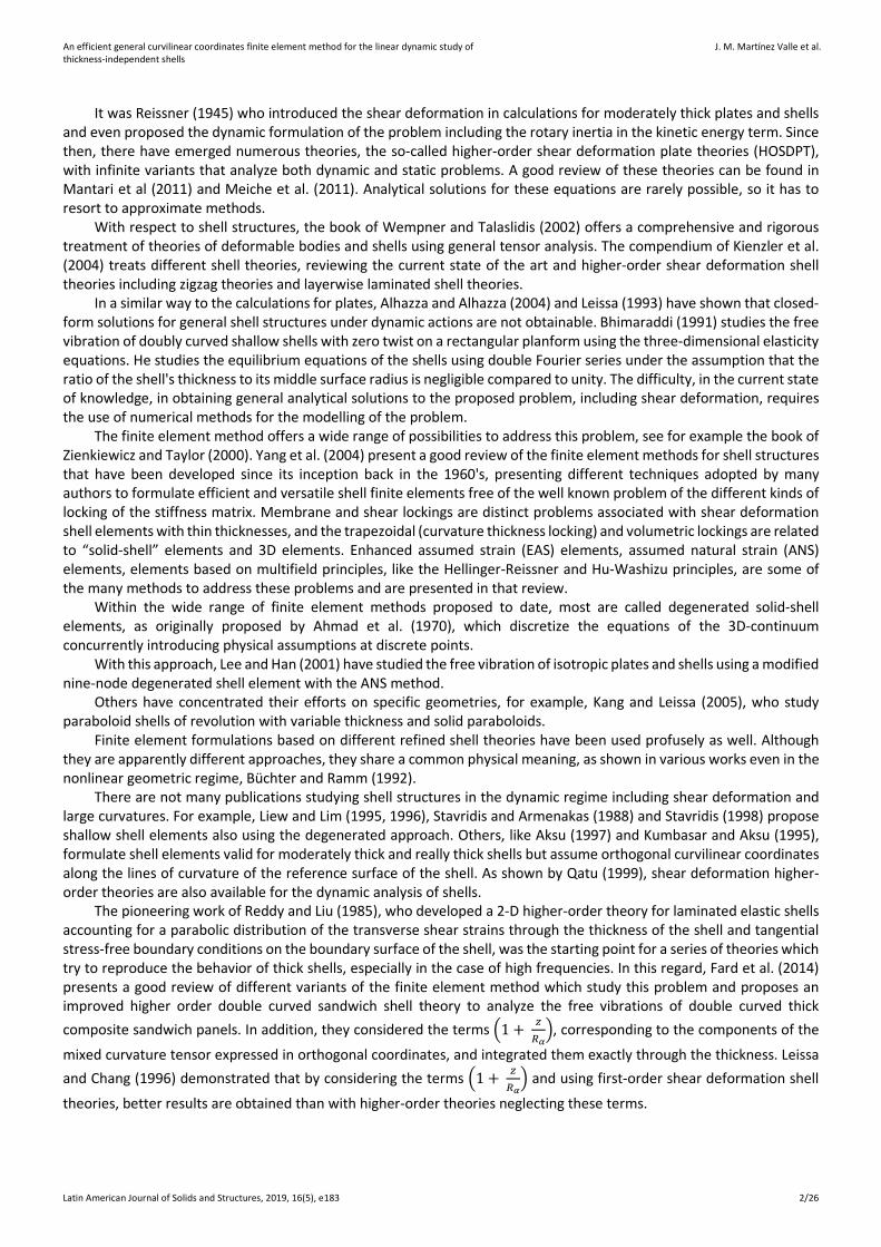
In order to work with shells, we admit that the reference surface of the shell can be parameterized by the curvilinear coordinates ( , )= 1 2αϑ α , not necessarily orthogonal.

Figure 1: Curvilinear local reference frame at the medium surface of the shell.

As we know, in the undeformed configuration of the shell, the position vector r of a point can be written as,

+= 30 3αr r a (1)

where 𝒓𝒓0 is the position vector of a point in the middle surface, 𝛼𝛼3 is the material coordinate measuring the length along the normal to the to the mid-surface, and 3a is the normal vector to the mid-surface, see Figure 1.

If we differentiate this expression, we obtain,




( ) ( ),,, = + = + = −= 3 3 30 3 3 bρ ρ

α α α ρα αα αα α δ αg r ar a a a (2)

where gα are the covariant base vectors which define the plane tangent to an arbitrary surface of the shell and bρα are the components of the mixed curvature tensor.

The relation between the metric tensors of the shell space gαβ and the middle surface aαβ takes the form,

( )= − +23 3g a 2 b cαβ αβ αβ αβα α (3)

where 𝑏𝑏𝛼𝛼𝛼𝛼 is the curvature tensor, the second fundamental form of the reference surface. and 𝑐𝑐𝛼𝛼𝛼𝛼 is the third fundamental form, a symmetrical tensor whose expression is,

=c b bγαβ α γβ (4)

The derivatives of the tangent vectors and the normal vector to the surface can be obtained from the Weingarten equations,

, = Γ + 3bγα β λ αβαβa a a (5)

, = −3 bλβ β λa a (6)

In these equations we have introduced the Christoffel symbols of the second kind Γγαβ , which are not tensors. Equation (2) can be written in a more compact way as,

=α αµg a (7)

where

:= ⊗iiµ g a (8)

µ is the so-called shifter tensor, the two point tensor which transforms the components of a vector in one coordinate system, the shell space, to the components of the same vector in another coordinate system, the reference surface, and has the expression,

.= − 3bρ ρα αµ δ α (9)

This contra-covariant tensor plays a fundamental role in the development of the theories of shells because it allows us to relate the tangent vectors to the medium surface and those related to any other surface of the shell (shell space).

For second order tensors, like the metric tensor, we have,

= a bij i j abg aµ µ (10)

If we consider, for example, a fourth order tensor, like the elastic constitutive tensor Cαβλµ , we can write

⊗ ⊗ ⊗ = ⊗ ⊗ ⊗C a a a a C g g g gαβλµ αβλµα β λ µ α β λ µ (11)

And hence,




( ) ( ) ( ) ( )− − − −= 1 1 1 1C Cα β λ µαβλµ ρστωρ σ τ ω

µ µ µ µ (12)

Similarly, one can obtain the relation between any geometric features of any surface of the shell and those of the middle surface through the shifter tensor.

The Christoffel symbols of the 2nd kind can be expressed as:

( ) ( ), ,· −Γ = = 1g g a a

γγ γ δ ξα β α δαβ β ξ

µ µ (13)

Now further developing this expression, we obtain

Γ = Γ = Γ =3 33 333 0γα α

(14)

Γ = Γ = Γ − t bγ γ γ γ λαβ βα αβ λ α βζ (15)

Γ = −3 b tcαβ αβ αβ (16)

Γ = −3 bα α λβ λ βζ (17)

with αλζ as the inverse of the shifter tensor,

= αγββ

αλ µζ δ (18)

=1 λα αγ

ββ λ γδ µµ

ζ (19)

These expressions are very interesting for developments concerning thick shells or those concerning high order theories, where it cannot be assumed that the geometrical properties of the shell space are not independent of the thickness.

To finish this section, it is very important for further developments, to know the expression of the differential volume 𝑑𝑑𝑑𝑑 in terms of known quantities of the middle surface.

By definition,

[ ]det= = = 1 2 3dV g g g g gαβ (20)

and taking into account the relation (7), we have,

[ ] ( ) ( ) ( )( ) ( )det , = = = = − − = − − = − = − +

23 3 3 3 3 3 31 2 3 3 31 1 2 2 1 1 2 2dV g g g g g b a b a a b b ae a b a 1 2 H Kρ ρ γ γ ρ ρ γ γ α α

αβ ρ γ ργ β βδ α δ α δ α δ α δ α α α (21)

where H y K are the mean and Gaussian curvature of the middle surface, invariants of the mixed curvature tensor. The relation between H and K can be established from,

− + =Ka 2Hb c 0αβ αβ αβ (22)

Hence, we can write,

( ) = = − +

23 3dV µdA 1 2H K dAα α (23)




which relates the differential of the volume to the area as a function of the mean and Gaussian curvature of the middle surface.

3 SHELLS KINEMATIC

The expression of the components of the linear strain tensor can be written as, Wempner (1982)

( )= +1 V V2αβ α β β αε

(24)

where V are the displacements of any point of the shell space and the double vertical bar denotes the covariant derivative with respect to a general basis of vectors tangent to a general surface of the shell space, not necessarily the middle shell surface. Recall that for a first order tensor, the covariant derivative has a more explicit form, given by,

,= −ΓV V Vγα β γαβα β (25)

As seen above, the tangent vectors to any surface of the shell 𝑽𝑽𝛼𝛼 and those tangents to the middle surface 𝒗𝒗𝛼𝛼 are related through the shifter tensor by

=V vβα α βµ (26)

=3 3V v (27)

At this point, we can express the covariant derivatives of the three dimensional components of the displacement vectors as a function of the two-dimensional components of the displacement vectors through the shifter tensor by,

( )= − 3V v b vλα λβα β λ βµ (28)

So we can rewrite the expression (24),

( ) ( )( )= − + −3 31 v b v v b v2

λ λαβ α λβ β λαλ β λ αµ µε (29)

where the single bar denotes the covariant derivative in the two-dimensional shell surface space. Considering the expression of the shifter tensor, the generalized strains can be written

( ) ( ) ( ) + − + − + =

33 3

1 1v v b v c v b v b v2 2

λ λαβ αβ αβ α βα β β α λ β λ α αε (30)

( ) ( ), ,= + = + +3 3 33 31 1V V v v b v2 2

λ λα α λ α α λα α µε (31)

,=33 3 3vε (32)

At this point we must introduce the corresponding kinematic hypothesis, which in our case it is a first shear deformation shell theory.

= + 3v uα α αα θ (33)

It physically indicates that after the deformation process, the fibers normal to the middle surface remain straight but not necessarily normal. After a more or less lengthy calculation, we obtain:




( ) ( ) ( ) ( ) ( ) = + − + + − − + + +

23 33 3

1 1 1u u b u b u b u c u b b 2 2 2

λ λ λ λαβ αβ β α αβ β λ α α λ βα β β α α β β α λ α λ βε θ θ α θ θ α∣ ∣ (34)

( ),= + +3 31 u b u2

λα α α α λθε (35)

So the linear strain tensor, Eαβ can be expressed in matrix form as follows,

( )

+

+ = =

23 33

3 33

1e2E

1 02 α

αβ

αβ αβ αβ ααβ α

α

ε α ρ

ζ

ε

ε ε

α κ ζ (36)

where,

( )+ −= 31e u u b u2αβ αβα β β α (37)

( )+ − −= + 31 b u b u c u2

λ λαβ β α αβα β β α λ α λ βρ θ θ (38)

( )= +1 b b 2

λ λαβ β λ α α λ βκ θ θ∣ ∣ (39)

, += + 3u b uλα α α α λζ θ (40)

Taking into account that for thin shells we can introduce the Kirchhoff-Love assumption, normals to the shell middle surface remain straight and normal to it during deformations and unstretched in length

( )= − +3u b uλα α λαθ (41)

In this case, displacements of a point of the shell space can be related to those in the reference surface by,

( )= − +33v u u b u aλ α

α α α λαα (42)

and the curvature tensor has the expression,

| |+= + + − 3 3

1 u b u b u b u b b u2

λ λ λ λαβ αβ β α λ β λ α α λ β α λβρ ∣ ∣ (43)

Note that in case we use this expression in finite element formulations, we have to impose first order continuity between shell elements, which is difficult to achieve for arbitrary geometries when using standard polynomials as shape functions.

4 STATEMENT OF THE PROBLEM.

There are different ways to get to the governing equations of the dynamic problem, either for analytical or approximate solutions. In the present work, we choose Hamilton's principle.

The problem to be solved is reduced to minimizing the functional:

=∫ *

time AL ad d dt 0δ ξ η∬ (44)




( )

( )

int

int

( ) * *

* *

= − + + =

+ − + + =

∫ ∫ ∫∫∫ ∫∫

∫ ∫∫∫ ∫∫

* 33

time time v AA

2 33 3

time v A

L dt T dV v v dA dt

1 V V V dV u u dA dt 02

β β

β β

αβ γ βα γ

α αβ γ βα α γ

δ δ π τ µ τ

δ ρ π

ν ν

ν ντ µ τ

∬ (45)

where 𝐿𝐿∗ is the called Lagrangian density function, which is defined as the difference between the kinetic energy T and the sum of the potential energy of deformation (strain energy density), intπ , plus the work of the external forces, defined in the previous equation. δ is the variation symbol, ρ is the material density and dots indicate differentiation with respect to time. *αβτ are the stress components corresponding to the specified edge tractions and $\nu_\beta$ are the components of the unit normal vector with respect to the mid-surface.

By differentiating the internal strain energy and the kinetic energy and discretizing, we reach the classical eigenvalue problem depending on the stiffness matrix and the mass matrix.

4.1 Strain energy of the shell element and equilibrium equations.

In order to formulate the stiffness matrix of the shell element, we develop an expression of the internal strain energy. In general, we can write,

int = ∫ ijij

V

1 E dV2

π τ (46)

where ijτ is the symmetric stress tensor and ijE is the linear strain tensor. Considering the expression (7) it can be written,

( )int

−

= + − +

∫ ∫h

2 23 3 3 1 23

hA2

1 E E a 1 2H K d d2

αβ ααβ απ τ τ α α α α (47)

Introducing the constitutive equations relating strains and stresses, for a linear elastic material, we have

= C Eαβ αβγδγδτ , =3 3 3

3C Eα α ββτ (48)

If this last expression is developed some integrals appear,

−= ∫

t32

0 t2

D C dαβγδ αβγδ µ α (49)

−= ∫

t3 32

1 t2

D C dαβγδ αβγδα µ α (50)

( )−

= ∫t

23 322 t

2

D C dαβγδ αβγδα µ α (51)

which are generalized constitutive equations for the shells appearing in the strain energy equation. Cαβγδ is the known elastic constant tensor (elasticity tensor) defined as:

− = + + − 1 2C a a a a a a

2 1αβγδ αδ βγ αγ βδ αβ γδν ν

ν (52)

where υ is the Poisson coefficient and aαδ is the metric tensor of the reference surface. For clarity, we can develop this last tensor equation by components (Voight notation),




( ) ( )( )( )

( ) ( ) ( )

=

− +

− +⋅

+

2 211 12 11 22 11 22

222 12 22

211 22 12

a a a a a a

C a a a

Sym a

1

1 12

a a2

υ υ

υ υ

(53)

Full expressions for the tensors 1Dαβγδ and 2Dαβγδ can be found integrating over the thickness,

( ) ( )( )( )−

+ + + +

= = + + −

∫t

3 321 t

2

2 a b b a 2 a b b a E D C d 42 1 a b b a

1

αγ βδ αγ βδ αδ βγ αδ βγ

αβγδ αβγδαβ γδ αβ γδ

α µ α ννν

(54)

( )( )( )

( )( )−

+ + +

= = + +

+ + + + −

∫t

23 322 t

2

3a b b 4b b 3a b bE D C d 3a b b 4b b 3a b b

2 12 3a b b 4b b 3a b b

1

αγ β τδ αγ βδ βδ α τγτ τ

αβγδ αβγδ αδ β τγ αδ βγ βγ α τδτ τ

αβ γ τδ αβ γδ γδ α τβτ τ

α µ αν

νν

(55)

Assuming that the shell is moderately thick, the above equation can be rewritten as,

int

−

≅ +

∫ ∫h

2 3 1 23

hA2

1 E E aµd d2

αβ ααβ απ τ τ α α (56)

If we define generalized stresses in the form,

( ) = = − + − = +

+ ≈

∫ ∫23

03 3

13

2

3n d D ed 1 2

h

DH K b

CD

αβ αβ αβγδ αβγδαβ

δα

αβ β

γ

β βα α α

β

αβ

β δ α γδγαβ

µµ α α α δτ ατ ρα

εκ (57)

( ) = = − + − = +

≈

∫ ∫11

23 3 3 3 3 3 3

2

3D

d 1 2H K b d

h C1

m D e

2

αβ β β βα α α

αβγδγδ

αβ αβ αβγδαβ

αβγδαβ

µµ α α α α δ α α ατ

ρ

τ

ρ

(58)

( ) ( ) = = − + −

= ≈

∫ ∫ 32 2 23 3 3 3

2

3 3

5

d 1 2H K b d

h C8

D0

m

e

αβ β β βα α α

αβγδγδ

αβ αβ

αβγδαβ

µµ α α α α δ α α α

κ

τ τ (59)

( ) = = − + ≈ ∫ ∫

23 3 3 3 3 33

3 3d 1 2H K dq hC Eβα αα αβµ α α ατ ατ (60)

the elastic strain energy of the shell element can be written

int = + +

+

∫

33 3 1 2

3

5

3A

h C8

1 hC he e C C hE E a1 0

d d2 2

αβγδ αβ αβγδγδ

γδ α βαβ γδ αβ γδ αβ α βπ ρ ρ κ α ακ

(61)

where the expressions of the various tensors were derived in the previous section and are given by equations (34) and (36).




In the theory of moderately thick shells, the tensor αβκ is usually not taken into account in the derivation of the

stiffness matrix. Note that the contribution in the strain energy of this term is multiplied by 5h

80and so we understand is

much less than the other terms. Bearing this in mind and neglecting this term, we can differentiate this last equation,

( ) ( )( ) ( )

int

,

Ω Ω = + + = + −

+ + − − + + + +

∫ ∫ ∫ ∫1 23

1 1 23 3

1n m q ad d n u u b u2

1 1m b u b u c u q u b u ad d2 2

αβ αβ α αβαβ αβ α αβα β β α

αβ λ λ α λβ α αβ α α α λα β β α λ α λ β

δπ δε δρ δς α α δ δ δ

δθ δθ δ δ δ δθ δ δ α α

(62)

The External virtual work by distributed load intensity 𝛿𝛿𝑊𝑊Ω and the external virtual work by shell edge resultant loads 𝛿𝛿𝑊𝑊Γ are given as:

( )Ω Ω= +∫ 3 1 23W p u p u ad dα

αδ δ δ α α (63)

( )Γ Γ= + + Γ∫ 3W n n u m n q n u dαβ αβ αα β α β αδ δ δθ δ

(64)

The finite element discretization of these functionals will be explained later, employing the MITC technique. Continuing with the usual process, the equilibrium equations can be deduced through the variational process:

( ) ,− − + = ttn b m b q p uαβ α γβ β γ ββ γ α γ αρ

(65)

,− + + + =3ttb n b b m q p wσγ σ δγ α

γσ γσ δ α ρ (66)

,− + = ttm q c Jαβ β ρα αθ (67)

where =3hJ

12ρ is the rotational inertia. With the consistent boundary conditions,

* *+ = stn b m Nαβ α δγ αβ γ αν ν

(68)

* = shq Qααν (69)

* = bem Mδγγ βν ν (70)

* = twm t Hδγλ βν (71)

Where beM is the bending moment resultant and twH is the twisting moment resultants. stN and shQ are the in-surface stretching resultant and shear resultant, respectively. The terms ,γ βν ν are the components of the unit normal vector with respect to the mid-surface, and tλ are the components of the unit tangent vector with respect to the same mid-surface.

4.2 Kinetic energy of the shell finite element in general curvilinear coordinates. Consistent and Lumped mass matrices.

The mass matrix of the finite element is necessary to study the dynamic problem. The lumped and consistent mass matrices are alternative formulations which can be used.




In this case, we propose to develop the consistent mass matrix, using the same shape functions for its discretization than those used for the geometry. As low order elements will be used for the interpolation of the variables, the solutions with the lumped mass matrix are very poor, and that is why we have opted for the consistent mass matrix that most authors agree in emphasizing for its elders benefits, Zienkiewicz and Taylor (2000).

The development of the mass matrix for a shell finite element in general curvilinear coordinates is more complex than for other elements such as three-dimensional elements, but conceptually it is developed in the same way, through the variation of the kinetic energy.

Our starting point is the definition of the kinetic energy,

·= ∫ ∫3

3

AdT d dA

αρ δ µ αR R

(72)

where R is the position vector of an arbitrary shell point in the deformed configuration. If we consider that the underlying shell theory allows for the transverse shear deformation effects, we can write,

= + N3d dd α0R R (73)

= + N30 α R R

(74)

Therefore the kinetic energy functional is:

( ) ( ) ( ) ( ),

= + ∂ + ∂ + ∂∫ ∫ ∫ ∫R R R N NN3 3 3

23 3 3 3 30 0 0 0

A elConstantTerm

Linear Term CuadraticTermC.T.L.T. C.T.

T d d dα α α

δ δ ρµ α ρα µ α ρ α µ α NR (75)

where C.T., L.T., and Q.T. stand for constant term, linear term, and quadratic term, respectively. We now carry out the interpolation of the variables involved:

, , ,= = = =

= = = =∑ ∑ ∑ ∑R R R N N4 4 4 4

0 i 0 i 0 i ii 1 i 1 1 i 1

0i

N N NN Nδ δ δ δ δ δ δ δ R N (76)

Introducing these expressions in (75),

( ) ( )

( ) ( )

( . .) ( . .)

( . .)

= = = =

= = =

= ⋅ + ⋅

+ ⋅ ⋅+

∑ ∑ ∑ ∑∫ ∫

∑ ∑ ∑∫

R R R N

N N

el el el el

elem elem

el el el

elem n

n m nN N N N

0 0 elem 0 elemn 1 m 1 n 1 m 1A A

ConstantTermLinear TermC.T.

L.T.

N N N0 elem

n 1 m 1 m 1A

Linear TermC.

m

T

m

n

.

T C T N N dA L T N N dA

L T N N dA

δ δ δ δ δ

δ δ δ δ

N R ( .)=∑ ∫

el

elem

Nelem

1 A

CuadraticTermC.T.

n mCuadraticT N N dA

(77)

The terms in equation (75) can be integrated without difficulty in the light of equation (7). Doing this, we find a matrix expression for the kinetic energy depending on the mass matrix, the nodal variables of the element and its second derivatives. The explicit expression of the mass matrix, M, is shown below.




+ + − −

+ − −

+ =

+ +

+

11 3 12 3 11 3 12 3

22 3 12 3 22 3

3

3 35 11 5 12

35 22

1 1 1 1a h h K a h h K 0 a Hh a Hh12 12 6 6

1 1 1a h h K 0 a Hh a Hh12 6 6

1h h K 0 0M 12

h 1 h 1h K a h K a12 80 12 80

h 1Sym h K a12 80

(78)

Note that the terms of the mass matrix depend on the mean and Gaussian curvature (H and K) and on the thickness of the shell, in contrast, for example, to a plate element, where all these quantities except the thickness are 0. If we introduce the Kirchhoff-Love assumption given by equation (43), a more refined expression for the mass matrix for thin shells can be found. At this point, we can solve equation (44).

5 LOCKING OF THE STIFFNESS MATRIX. MIXED INTERPOLATION OF TENSORIAL COMPONENTS

Once an expression for the internal energy of the shell element has been deduced, with the inclusion of the shear strain effects and the kinetic energy necessary for the dynamic formulation of the problem, we need to discretize the middle surface of the shell by the isoparametric formulation, to subsequently integrate over the thickness.

For the interpolation of the displacements u within an element, bilinear shape functions have been used,

( ),=

= ∑ i 1 24

i 1N ξ ξu iδ

(79)

where 𝜹𝜹𝒊𝒊 is the generalized nodal displacement vector, i.e. ( , , , , )=i 1 2 3 1 2u u uδ θ θ and ,1 2ξ ξ are the isoparametric coordinates. One of the advantages of the proposed formulation is that the basis vectors and other geometric parameters of the

surface are known exactly. As mentioned in the introduction, when the thickness of the shell becomes thinner, the shell elements suffer from

the so-called shear locking (and membrane locking if the element are curved), causing spurious shear and membrane strains in bending dominated problems.

To circumvent this drawback, we turn to a well known technique originally proposed by Dvorkin and Bathe (1984); Bathe and Dvorkin (1986) for elements of low order, and Bucalem and Bathe (1993) for higher order elements, called mixed interpolation of tensorial components (MITC𝑛𝑛 , where n stands for the number of nodes in the element), which can be encompassed within assumed strain methods. In general, the covariant strains are individually interpolated in MITC𝑛𝑛 finite elements, where a set of 𝑛𝑛𝑖𝑖𝑖𝑖tying points associated to each strain component 𝐸𝐸𝑖𝑖𝑖𝑖 is adopted.

Hence, the shear components of the linear strain tensor (in covariant form) are interpolated so that

( ) ( ), , ,=

= ∑p

AS DI1 2 1k 2k

k 1k E tE αβ

αβ αβΛ ξ ξ ξ ξ (80)

In this equation, the assumed strains 𝐸𝐸𝛼𝛼𝛼𝛼𝐴𝐴𝐴𝐴 can be computed from the strains which have been interpolated through

the shape functions Λ𝑘𝑘𝛼𝛼𝛼𝛼(𝜉𝜉1, 𝜉𝜉2) . These shape functions depend on the isoparametric coordinates (𝜉𝜉1, 𝜉𝜉2) and

correspond to the strain component (α,β) evaluated at point k. The so-called tying points defined on the shell midsurface with coordinates (𝜉𝜉𝑃𝑃, 𝜉𝜉𝑃𝑃)define the assumed covariant strain components. p is the number of tying points for the covariant strain component AS

Eαβ and ( ),1 2kαβΛ ξ ξ are the assumed interpolation functions, satisfying,

( ),Λ = Λ = kll lk klαβ αβ ξ ξ δ

(81)

We must note that this procedure is carried out at the elemental level for each individual element.




For more details regarding this formulation, we refer to the above-mentioned papers. In our case, the components of the linear strain tensor are given by equations (34) and (36). If we develop these tensor equations, the relation between strains and displacements can be written as,

∂ − Γ −Γ −

−Γ ∂ −Γ −

∂ − Γ ∂ − Γ

− ∂ + Γ − ∂ + Γ ∂ −Γ −Γ

− ∂ + Γ − ∂ + Γ −Γ ∂ −Γ

− ∂ + Γ − ∂ + Γ −

−

∂ + Γ

=

1 211 11

1 222 22

1 212 12

1 1 2 2 1 21 1 1 1 1 1 1 11

1 11

2 22

2 1 12

1 1 1 1 111 1 2 2 1 22 2 2 2 2 2 2 22 221 1 22 2 1 2 21 21 1 2

2 2 2 2

1 1

2

0 0

0 0

2 0 0

B

b

b

2 2 b

b b b b b b

b b b b b b

b b b b

b b

α α αα α

α α αα

αα

α

α

α

ααα

∂ − Γ ∂ − Γ − ∂ + Γ

∂

∂

21 1 2

1 12 122 21 1 2

1 22 21 21 1

2 2 12

2

1

b b 2 2b b

b b

1 0b b

2

0 1

α αα

αα

(82)

with

=

11

221

122

11

221

122

23

13

ee

ue

uB w

ρρ

θρ

θζζ

(83)

which would be properly interpolated by the chosen shape functions. For the construction of the stiffness matrix, note that we use ASEαβ instead of DIEαβ defined by the last equation. Also, it is important to remark that if we had considered higher order moments defined by the tensor αβκ , this last matrix would have to contain its components adequately ordered.

,

− ∂ + Γ − ∂ + Γ = − + Γ − ∂ + Γ

− ∂ + Γ − ∂ + Γ − ∂ + Γ − ∂ + Γ

1 1 2 21 1 1 1 1 1 1 111

11 I 1 2 222 2 2 2 2 2 2 2 2

21 1 2 212 2 1 2 1 2 1 2 11 2 2 21 2 1 2 1 2 1 2

b b b b

b N b b b

b b b b

b b b b

α αα α

α αα α

α αα α

α αα α

θθ

κκκ

(84)

It should be noted that the geometric characteristics of the surface are defined only at the nodes of the finite element, and that due to the invariance of the internal energy we can operate directly on the tensorial components without having to resort to the physical components of the variables.

6 RESULTS AND DISCUSSION

To test the validity of these results, we compared the results from using the new shell element with the results obtained by other authors with several types of shell structures: hyperbolic paraboloid shells as well as cylindrical, spherical and elliptic parabolioid shells. In general, doubly-curved shells pose very stringent tests to validate solutions, whether they are static or dynamic. A considerable number of examples, including clamped and simply supported isotropic shells with a wide range of ratios h/R and L/R, will be investigated.

The comparison of the present formulation is made with regard to the original test case, and also with the four-node shell model based on the degenerated solid approach developed by Dvorkin and Bathe (1984). In all cases, the consistent mass matrices have been used, and finite element models have been discretized with 50 by 50 elements in




the x and y directions respectively. Throughout these examples, we show the efficiency and versatility of the present formulation.

6.1 Example 1: Corner point supported thin hyperbolic paraboloid

To begin with, Narita and Leissa (1984) and Chakravorty and Bandyopadhyay (1995) and Chakravorty et al. (1995) study the free vibration of several types of surfaces incluiding the hyperbolic paraboloid. The hyperbolic paraboloid test, a surface with negative Gaussian curvature, is quite demanding both surface type (doubly curved shell) and the boundary conditions.

The corner point supported thin hyperbolic paraboloid test of Figure 2 involves a surface with a negative Gaussian curvature, and is quite demanding both as to the type of surface involved (doubly curved shell) and its boundary conditions. The data of the problem is: square planform 1 x 1 m side, constant thickness of h=0.01 m., equal radii of curvature and opposite in sign .= =y xR R 2m , Young modulus, . /= 6 2E 10 92 10 N m Poisson's ratio ,= 0 3υ and density

/= 3100 kg mρ .

Figure 2: Corner point supported thin hyperbolic paraboloid with curved edges (Example 1, Table 1).

Table 1 presents the frequency associated with the first mode of vibration of the hyperbolic paraboloid according to results obtained by the above-named authors.

The frequency associated with the first mode of vibration of the hyperbolic paraboloid according the new formulation is 17, 21rad / s. The results obtained by the above-named authors are:

Table 1: Frequency associated with the first mode of vibration of the corner point supported thin hyperbolic paraboloid with curved edges. Comparison with Narita and Leissa (1984), Chakravorty and Bandyopadhyay (1995), and the degenerated solid approach of

Dvorkin and Bathe (1984).

Narita and Leissa (1984) 17.16 rad/s

Chakravorty and Bandyopadhyay (1995) 17.25 rad/s Deg. Sol. Shell 17.31 rad/s

Proposed 17.21 rad/s

The first three modes of vibration for the corner point supported thin hyperbolic paraboloid with curved edges are depicted in Figure 3:




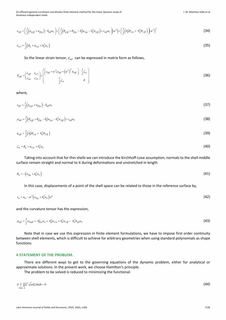
Figure 3: First (a), second (b), and third (c) mode of vibration for the thin hyperbolic paraboloid simply supported at the corners

(Example 1, Table 1).

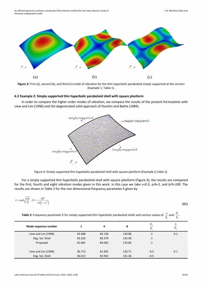
6.2 Example 2: Simply supported thin hyperbolic paraboloid shell with square planform

In order to compare the higher order modes of vibration, we compare the results of the present formulation with Liew and Lim (1996) and the degenerated solid approach of Dvorkin and Bathe (1984).

Figure 4: Simply supported thin hyperbolic paraboloid shell with square planform (Example 2,Table 2).

For a simply supported thin hyperbolic paraboloid shell with square planform (Figure 4), the results are compared for the first, fourth and eight vibration modes given in this work. In this case we take ν=0.3, a⁄b=1, and b⁄h=100. The results are shown in Table 2 for the non dimensional frequency parameter λ given by

( ) , = =

−

3

2h Ehab D

D 12 1ρλ ω

υ

(85)

Table 2: Frequency parameter λ for simply supported thin hyperbolic paraboloid shells and various values of y

bR

and y

x

RR

.

Mode sequence number 1 4 8 y

x

RR

y

bR

Liew and Lim [1996] 42.688 83.136 130.86 -1 0.1 Deg. Sol. Shell 43.326 84.379 135.40 -1

Proposed 42.681 84.062 133.80 -1

Liew and Lim [1996] 36.713 81.902 130.71 -0.5 0.1 Deg. Sol. Shell 36.012 83.942 131.46 -0.5





x

RR

y

bR

Proposed 36.715 82.887 133.52 -0.5


Proposed 103.42 110.79 151.22 -1

Liew and Lim [1996] 75.152 102.10 148.35 -0.5 0.3 Deg. Sol. Shell 74.965 100.89 147.13 -0.5

Proposed 75.082 102.25 148.99 -0.5


Proposed 145.62 160.34 196.79 -1

Liew and Lim [1996] 105.48 136.48 177.97 -0.5 O.5

Deg. Sol. Shell 105.71 135.93 178.74 Proposed 104.66 137.11 178.99

(ν=0.3,, a⁄b=1, and b⁄h=100). Comparison with Liew and Lim (1996) and the degenerated solid approach of Dvorkin and Bathe (1984).

6.2.1 Mesh convergence analysis for thin hyperbolic paraboloid shell

A mesh convergence analysis has been performed to evaluate the performance of the proposed formulation. Table 3 presents the frequency parameter λ for simply supported thin hyperbolic paraboloid shells.

Table 3: Mesh convergence analysis of the proposed formulation. Parameter for simply supported thin hyperbolic paraboloid shells

and various values of y

bR

and y

x

RR

. (ν=0.3, a⁄b=1, and b⁄h=100)


x

RR

y

bR

Present (50*50) 42.681 84.062 133.80 -1 0.1

(40*40) 42.681 84.071 133.81 (30*30) 42.683 84.075 133.84 (20*20) 42.686 84.082 133.89 (10*10) 42.697 84.106 134.59

(5*5) 43.041 85.127 136.24

Present 36.715 82.887 133.52 -0.5 0.1 (40*40) 36.715 82.892 133.54 (30*30) 36.718 82.898 133.55 (20*20) 36.720 82.901 133.56 (10*10) 36.735 83.047 134.72

(5*5) 37.182 83.966 135.93

Present 103.42 110.79 151.22 -1 0.3 (40*40) 103.42 110.80 151.23 (30*30) 103.43 110.81 151.25 (20*20) 103.43 110.82 151.30 (10*10) 103.78 111.24 152.09

(5*5) 104.59 112.36 154.00





x

RR

y

bR

Present 75.082 102.25 148.99 -0.5 0.3 (40*40) 75.082 102.28 149.02 (30*30) 75.084 102.29 149.03 (20*20) 75.087 102.31 149.03 (10*10) 75.580 102.82 149.96

(5*5) 75.894 103.56 151.86

Present 145.62 160.34 196.79 -1 0.5 (40*40) 145.62 160.36 196.80 (30*30) 145.63 160.36 196.81 (20*20) 145.63 160.38 196.82 (10*10) 145.99 160.42 197.59

(5*5) 146.46 161.68 199.33

Present 104.66 137.11 178.99 -0.5 0.5 (40*40) 104.66 137.12 179.02 (30*30) 104.67 137.12 179.02 (20*20) 104.68 137.14 179.04 (10*10) 104.71 137.20 180.47

(5*5) 105.34 138.09 182.90

6.2.2 Vibration analysis for thin hyperbolic paraboloid shell with distorted meshes

To evaluate the proposed formulation for distorted meshes, the structured meshes (consisting in elements of size L x L) where distorted by different fractions of the element length L, for values 0.1L, 0.2L, and 0.4L, see Figure 5. Table 4 presents the frequency parameter λ for simply supported thin hyperbolic paraboloid shells with distorted mesh.

Figure 5: Test with distorted meshes. Simply supported thin hyperbolic paraboloid shells, with mesh distorted by different fractions

of the element length: (a) 0.1L, (b) 0.2L, and (c) 0.4L. (Table 4).

Table 4: Vibration analysis for distorted meshes, for the simply supported thin hyperbolic paraboloid shells. Parameter λ for the first frequency mode (ν=0.3, a⁄b=1, and b⁄h=100). 50 x 50 element mesh distorted with 𝑑𝑑𝑑𝑑𝑑𝑑𝑑𝑑𝑓𝑓𝑓𝑓𝑓𝑓𝑓𝑓 of 0.1L, 0.2L, and 0.4L. Comparison with

the deg. solid approach of Dvorkin and Bathe (1984).

0.1L 0.2L 0.4L Undistorted mesh

y

x

RR

y

bR

Proposed finite element 42.681 42.681 42.682 42.681 -1 0.1

Deg. Solid Shell 43.329 43.704 43.981 43.326 -1

Proposed finite element 36.715 36.715 36.717 36.715 -0.5 0.1




0.1L 0.2L 0.4L Undistorted mesh

y

x

RR

y

bR

Deg. Solid Shell 36.014 36.126 36.532 36.012 -0.5

Proposed finite element 103.42 103.42 103.43 103.42 -1 0.3

Deg. Solid Shell 103.42 103.49 103.69 103.41 -1

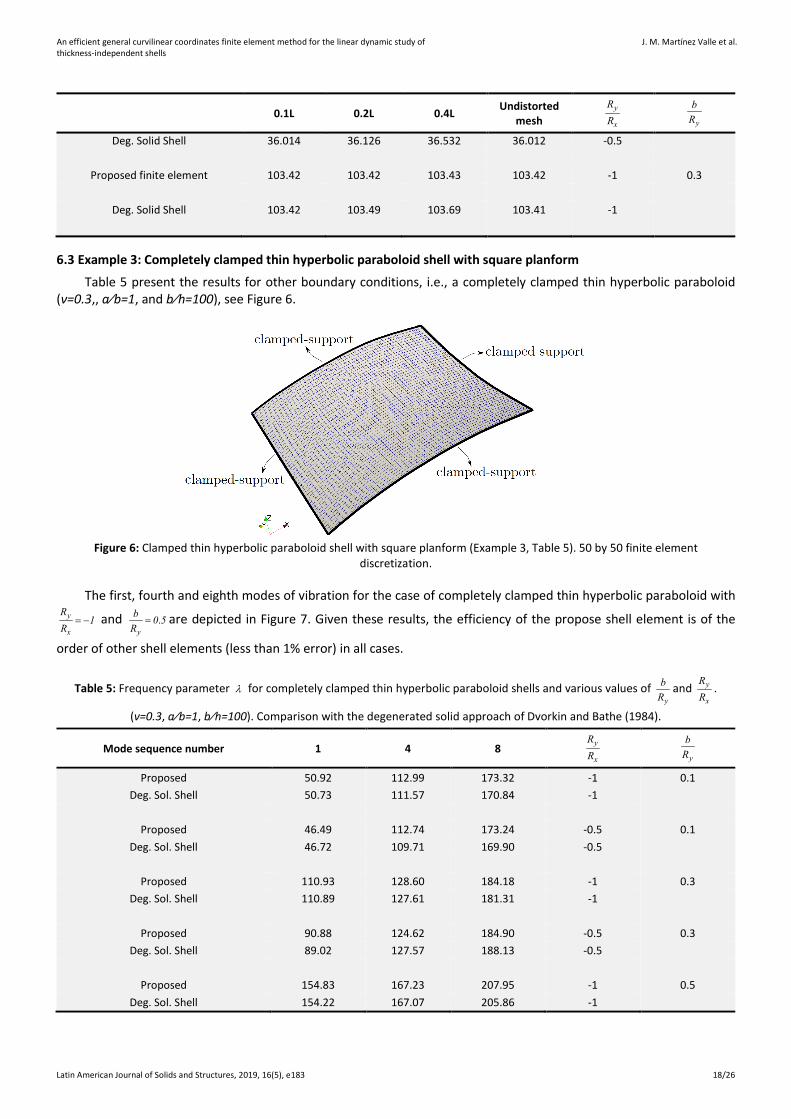
6.3 Example 3: Completely clamped thin hyperbolic paraboloid shell with square planform

Table 5 present the results for other boundary conditions, i.e., a completely clamped thin hyperbolic paraboloid (ν=0.3,, a⁄b=1, and b⁄h=100), see Figure 6.

Figure 6: Clamped thin hyperbolic paraboloid shell with square planform (Example 3, Table 5). 50 by 50 finite element

discretization.

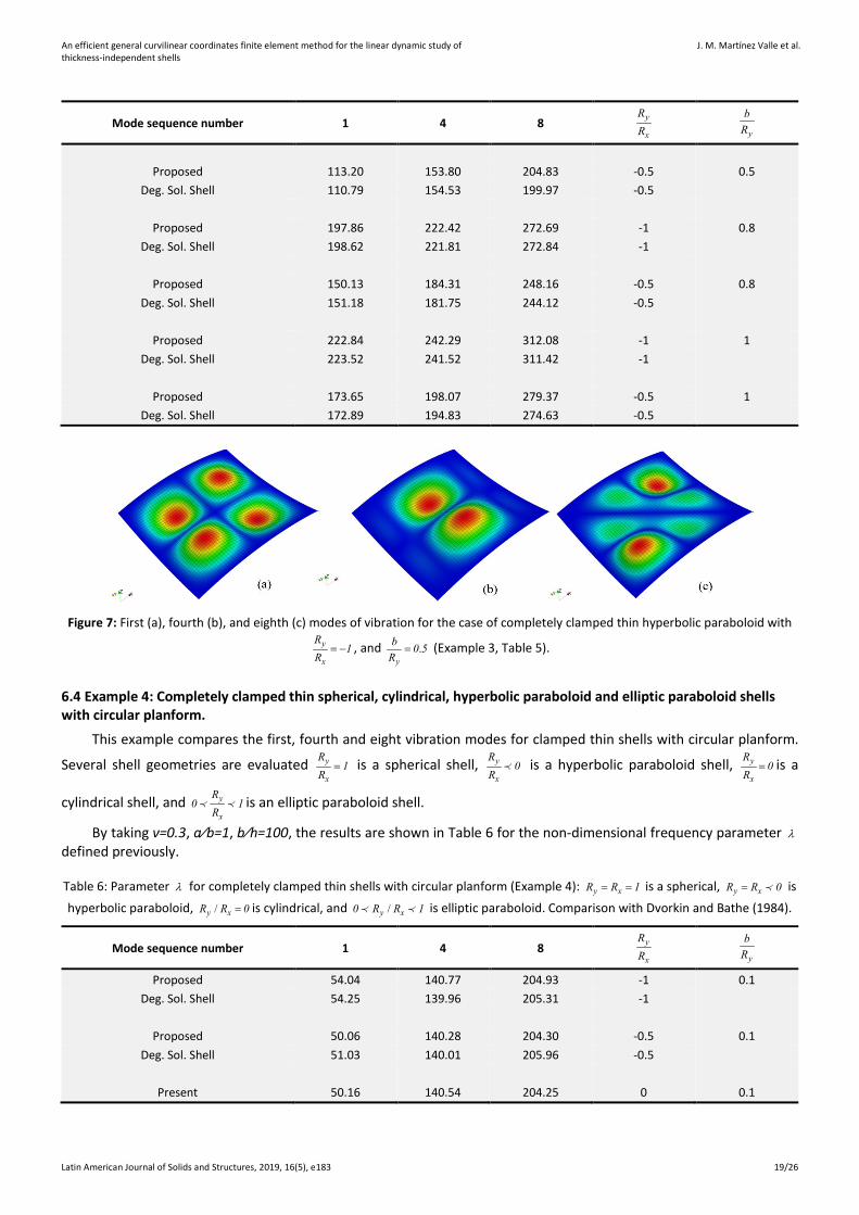
The first, fourth and eighth modes of vibration for the case of completely clamped thin hyperbolic paraboloid with

= −y

x

R1

R and .=

y

b 0 5R

are depicted in Figure 7. Given these results, the efficiency of the propose shell element is of the

order of other shell elements (less than 1% error) in all cases.

Table 5: Frequency parameter λ for completely clamped thin hyperbolic paraboloid shells and various values of y

bR

and y

x

RR

.

(ν=0.3, a⁄b=1, b⁄h=100). Comparison with the degenerated solid approach of Dvorkin and Bathe (1984).


x

RR

y

bR

Proposed 50.92 112.99 173.32 -1 0.1 Deg. Sol. Shell 50.73 111.57 170.84 -1

Proposed 46.49 112.74 173.24 -0.5 0.1

Deg. Sol. Shell 46.72 109.71 169.90 -0.5


Proposed 90.88 124.62 184.90 -0.5 0.3

Deg. Sol. Shell 89.02 127.57 188.13 -0.5






x

RR

y

bR

Proposed 113.20 153.80 204.83 -0.5 0.5

Deg. Sol. Shell 110.79 154.53 199.97 -0.5


Proposed 150.13 184.31 248.16 -0.5 0.8

Deg. Sol. Shell 151.18 181.75 244.12 -0.5

Proposed 222.84 242.29 312.08 -1 1 Deg. Sol. Shell 223.52 241.52 311.42 -1

Proposed 173.65 198.07 279.37 -0.5 1

Deg. Sol. Shell 172.89 194.83 274.63 -0.5

Figure 7: First (a), fourth (b), and eighth (c) modes of vibration for the case of completely clamped thin hyperbolic paraboloid with

= −y

x

R1

R, and .=

y

b 0 5R

(Example 3, Table 5).

6.4 Example 4: Completely clamped thin spherical, cylindrical, hyperbolic paraboloid and elliptic paraboloid shells with circular planform.

This example compares the first, fourth and eight vibration modes for clamped thin shells with circular planform.

Several shell geometries are evaluated =y

x

R1

R is a spherical shell, y

x

R0

R is a hyperbolic paraboloid shell, =y

x

R0

Ris a

cylindrical shell, and y

x

R0 1

R is an elliptic paraboloid shell.

By taking ν=0.3, a⁄b=1, b⁄h=100, the results are shown in Table 6 for the non-dimensional frequency parameter λdefined previously.

Table 6: Parameter λ for completely clamped thin shells with circular planform (Example 4): = =y xR R 1 is a spherical, =y xR R 0 is

hyperbolic paraboloid, /y xR R 0= is cylindrical, and /y x0 R R 1 is elliptic paraboloid. Comparison with Dvorkin and Bathe (1984).


x

RR

y

bR


Proposed 50.06 140.28 204.30 -0.5 0.1

Deg. Sol. Shell 51.03 140.01 205.96 -0.5

Present 50.16 140.54 204.25 0 0.1





x

RR

y

bR

Deg. Sol. Shell 48.97 141.65 204.78 0

Present 54.34 141.55 204.78 0.5 0.1 Deg. Sol. Shell 53.77 140.86 204.21 0.5

Present 61.73 143.30 205.93 1 0.1

Deg. Sol. Shell 60.43 144.21 205.05 1

Present 111.80 153.72 217.54 -1 0.3 Deg. Sol. Shell 111.71 152.69 216.88 -1

Present 94.025 149.69 212.98 -0.5 0.3

Deg. Sol. Shell 93.71 150.11 213.84 -0.5

Present 93.48 151.71 212.52 0 0.3 Deg. Sol. Shell 92.91 152.25 213.07 0

Present 108.59 159.70 217.36 0.5 0.3

Deg. Sol. Shell 107.82 158.01 216.39 0.5

Present 135.54 172.99 226.53 1 0.3 Deg. Sol. Shell 133.85 174.29 225.77 1

Present 164.31 175.38 238.89 -1 0.5

Deg. Sol. Shell 162.02 177.13 239.52 -1

Present 121.86 165.70 229.12 -0.5 0.5 Deg. Sol. Shell 120.37 163.94 228.63 -0.5

Present 108.74 170.65 226.87 0 0.5

Deg. Sol. Shell 106.39 169.20 225.74 0

Present 139.49 188.52 238.80 0.5 0.5 Deg. Sol. Shell 137.30 190.80 240.07 0.5

Present 192.79 218.40 262.66 1 0.5

Deg. Sol. Shell 190.51 217.65 262.04 1

6.5 Example 5: Completely clamped moderately thick hyperbolic paraboloid shells

In order to compare the results with moderately thick shells, we use the parameter λ´, given by

´= habEρλ ω (86)

If we analyze again the completely clamped hyperbolic paraboloid but with a relation b⁄h=10, then within the range of moderately thick shells, (ν=0.3, a⁄b=1, b⁄h=10), we obtain the results presented in Table 7.




Table 7: Frequency parameter ´λ for completely clamped moderately thick hyperbolic paraboloid shells and various values of bRy

and RyRx

(Example 5), (ν=0.3, a⁄b=1, b⁄h=10). Comparison with the degenerated solid approach of Dvorkin and Bathe (1984).


x

RR

y

bR


Present 0.996 2.679 3.732 -0.5 0.1

Deg. Sol. Shell 0.986 2.649 3.713 -0.5


Present 1.019 2.666 3.730 -0.5 0.3

Deg. Sol. Shell 1.021 2.687 3.734 -0.5


Present 1.068 2.651 3.723 -0.5 0.5

Deg. Sol. Shell 1.069 2.712 3.742 -0.5


Present 1.180 2.609 3.705 -0.5 0.8

Deg. Sol. Shell 1.186 2.615 3.674 -0.5

Present 1.383 2.521 3.620 -1 1 Deg. Sol. Shell 1.384 2.513 3.599 -1

Present 1.260 2.582 3.692 -0.5 1

Deg. Sol. Shell 1.255 2.601 3.722 -0.5

The good agreement between the two result sets becomes worst as the shallowness ratio bRy

increases. The reason

is that the present approach is based on a general shell theory, whereas in in Liew and Lim (1996) a shallow shell formulation is considered. The first, fourth and eighth modes of vibration for the completely clamped moderately thick

hyperbolic paraboloid with .= −Ry 0 5Rx

, and .=b 0 8

Ryare depicted in Figure 8.

Figure 8: First (a), fourth (b), and eighth (c) modes of vibration for the case of completely clamped moderately thick hyperbolic

paraboloid with .= −Ry 0 5Rx

, and .=b 0 8

Ry (Example 5, Table 7).




6.6 Example 6: Simply supported thin cylindrical, spherical, and elliptic paraboloid shells

To conclude this work, we also study the natural frequencies of other kinds of surfaces, such as cylindrical, spherical, and elliptic paraboloid shells. In the following table, the boundary conditions are also those of a simply supported shell in order to compare them with the analysis of Liew and Lim [1996], Table 8, (ν=0.3, a⁄b=1, b⁄h=100).

Table 8: Frequency parameter λ for simply supported thin cylindrical shells and spherical shells (Example 6) for various values of bRy

and RyRx

(ν=0.3, a⁄b=1, b⁄h=100). Comparison with Liew and Lim (1996) and the degenerated solid approach of Dvorkin and Bathe

(1984).


x

RR

y

bR

Liew and Lim [1996] 36.841 82.302 131.11 0 0.1 Deg. Sol. Shell 36.024 81.687 130.85 0

Proposed 36.019 82.411 133.57 0

Liew and Lim [1996] 43.027 84.316 132.05 0.5 0.1 Deg. Sol. Shell 44.350 86.062 134.80 0.5

Proposed 42.208 85.154 134.21 0.5


Proposed 52.677 88.906 134.62 1


Proposed 66.152 106.02 153.73 0


Proposed 86.000 118.85 160.29 0.5


Proposed 119.65 141.52 170.83 1


Proposed 87.851 142.74 183.62 0


Proposed 128.63 167.28 202.15 0.5

Liew and Lim [1996] 188.59 201.27 239.87 1 0.5 Deg. Sol. Shell 193.56 199.93 239.52

Proposed 200.01 202.36 241.24

Finally, in Table 9 and Table 10, we present different results for completely clamped spherical and cylindrical shells. The results show no significant differences from those obtained while using the other finite elements. We can see that the results obtained with the classical formulation are closer to the shallow shell theory whereas the new formulation is closer to the deep shell theory. For simply supported shells, it can be seen that higher frequencies vary linearly with the




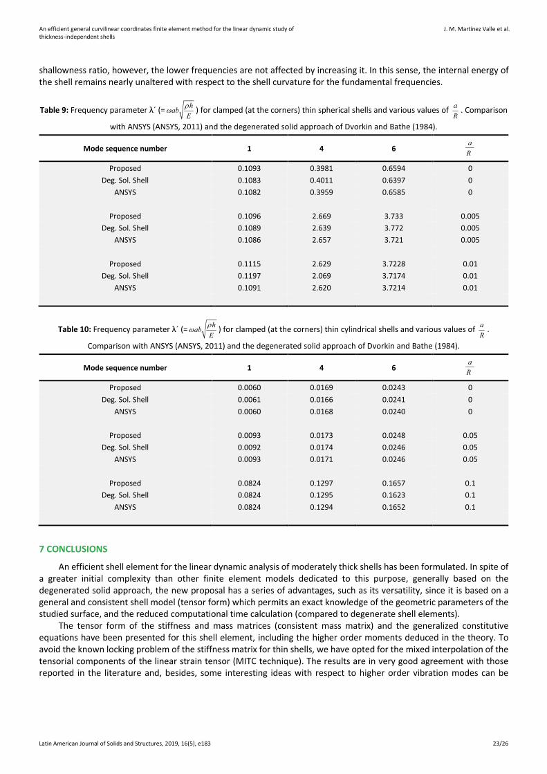
shallowness ratio, however, the lower frequencies are not affected by increasing it. In this sense, the internal energy of the shell remains nearly unaltered with respect to the shell curvature for the fundamental frequencies.

Table 9: Frequency parameter λ´ (= habEρω ) for clamped (at the corners) thin spherical shells and various values of a

R. Comparison

with ANSYS (ANSYS, 2011) and the degenerated solid approach of Dvorkin and Bathe (1984).

Mode sequence number 1 4 6 aR

Proposed 0.1093 0.3981 0.6594 0 Deg. Sol. Shell 0.1083 0.4011 0.6397 0

ANSYS 0.1082 0.3959 0.6585 0

Proposed 0.1096 2.669 3.733 0.005 Deg. Sol. Shell 0.1089 2.639 3.772 0.005

ANSYS 0.1086 2.657 3.721 0.005


ANSYS 0.1091 2.620 3.7214 0.01

Table 10: Frequency parameter λ´ (= habEρω ) for clamped (at the corners) thin cylindrical shells and various values of a

R.

Comparison with ANSYS (ANSYS, 2011) and the degenerated solid approach of Dvorkin and Bathe (1984).

Mode sequence number 1 4 6 aR

Proposed 0.0060 0.0169 0.0243 0 Deg. Sol. Shell 0.0061 0.0166 0.0241 0

ANSYS 0.0060 0.0168 0.0240 0


ANSYS 0.0093 0.0171 0.0246 0.05


ANSYS 0.0824 0.1294 0.1652 0.1

7 CONCLUSIONS

An efficient shell element for the linear dynamic analysis of moderately thick shells has been formulated. In spite of a greater initial complexity than other finite element models dedicated to this purpose, generally based on the degenerated solid approach, the new proposal has a series of advantages, such as its versatility, since it is based on a general and consistent shell model (tensor form) which permits an exact knowledge of the geometric parameters of the studied surface, and the reduced computational time calculation (compared to degenerate shell elements).

The tensor form of the stiffness and mass matrices (consistent mass matrix) and the generalized constitutive equations have been presented for this shell element, including the higher order moments deduced in the theory. To avoid the known locking problem of the stiffness matrix for thin shells, we have opted for the mixed interpolation of the tensorial components of the linear strain tensor (MITC technique). The results are in very good agreement with those reported in the literature and, besides, some interesting ideas with respect to higher order vibration modes can be




highlighted. In this sense, the differences with other competitive finite elements become greater for thicker shells and for higher values of the ratios

y

bR

.

Indeed, we have focused on several kinds of surfaces, such as cylindrical, spherical, elliptic paraboloid and doubly curved shells, with a wide range of shallowness ratios and different boundary conditions, constituting strict tests for validating the new finite element, as well as due to the lack of results for non-shallow and thick shells (deep shells). The extension of this general dynamic formulation to other attractive problems in structural mechanics like material and geometric nonlinear shell analysis or applications to composite shell models is direct and will be presented in future works.

8 ACKNOWLEDGMENTS

The authors gratefully acknowledge financial support from the University of Córdoba in Spain (Plan Propio de Investigación de la Universidad de Córdoba y del Programa Operativo de fondos FEDER Andalucía), and CONICET (Argentine Council for Scientific and Technical Research). A. E. Albanesi also acknowledges the National Technological University of Argentina (UTN) for Grants PID ENUTNFE0004405 and PID MAUTIFE0005270TC, and the National Agency of Scientific and Technological Promotion of Argentina (ANPCYT) for the Grant PICT2015-3396.

Author Contributions: Conceptualization, JM Martínez Valle; Methodology, JM Martínez Valle; Investigation, JM Martínez Valle, A Albanesi and V Fachinotti; Funding acquisition, JM Martínez Valle; Resources, JM Martínez Valle; A Albanesi and V Fachinotti; Software, JM Martínez Valle and A Albanesi; Supervision, JM Martínez Valle; A Albanesi and V Fachinotti; Validation, JM Martínez Valle and A Albanesi; Writing – original draft, JM Martínez Valle; Writing – review & editing, JM Martínez Valle and A Albanesi.

Editor: Marco L. Bittencourt.

References

ANSYS, (2011). Academic Research Mechanical, Release 14, Help System.

Aksu, T., (1997). A finite element formulation for free vibration analysis of shells of general shape. Computers and Structures 65, 687-694.

Ahmad, S., Irons B., and Zienkiewicz, O.C., (1970). Analysis of thick and thin shell structures by curved finite elements. International Journal for Numerical Methods in Engineering 2, 419-451.

Alhazza, K, and Alhazza, A., (2004). A review of the vibrations of plates and shells. The Shock and Vibration Digest; 36(5):377–395.

Bathe, K.J., and Dvorkin, E.N., (1986). A formulation of general shell elements – the use of mixed interpolation of tensorial components. International Journal for Numerical methods in Engineering. 22:697–722.

Bhimaraddi, A., (1991). Free vibration analysis of doubly curved shallow shells on rectangular planform using three-dimensional elasticity theory. International Journal of Solids and Structures. 27, 897-913.

Bucalem, M.L., y Bathe, K.J., (1993). Higher-order MITC general shells elements. International Journal for Numerical methods in Engineering. 36:3729–3754.

Büchter, N., Ramm, E., (1992). Shell Theory versus Degeneration – A Comparison in Large Rotation Finite Element Analysis. International Journal for Numerical methods in Engineering 34, 39-59.

Chakravorty, D., and Bandyopadhyay, J., (1995). On the free vibration of shallow shells. Journal of Sound and Vibration, 185(4):673–684.

Chakravorty, D., Bandyopadhyay, J.N., and Sinha, P.K., (1995). Free vibration of point-supported laminated doubly curved shells-a finite element approach. Comput Struct, 54(2):191–8.




Chapelle, D., and Bathe, K.J., (1998). Fundamental considerations for the finite element analysis of shell structures. Computers & Structures. 66 (1) January: 19-36.

Chapelle, D., Suarez IP., (2008). Detailed reliability assessment of triangular MITC elements for thin shells. Computers and Structures. 86(23– 24):2192–2202.

Dvorkin E. N., and Bathe K.-J., (1984). A continuum mechanics based four-node shell element for general nonlinear analysis. Eng. Comput. 1(1):77–88.

Fard, K. M., Livani M.; Faramarz Ashenai Ghasemi., (2014). Improved high order free vibration analysis of thick double curved sandwich panels with transversely flexible cores. Latin American Journal of Solids and Structures. 11: 2284–2307.

Germain, S. (1821). Recherches sur la the’orie des surfaces e’lastiques Mme. V. Courcier edt., Paris.

Kang J.H., Leissa, A.W., (2005). Free vibration analysis of complete paraboloidal shells of revolution with variable thickness and solid paraboloids from a three-dimensional theory Comput. Struct. 83: 2594-2608.

Kienzler, R., Altenbach, H. and Ott, I., (2004). Theories of Plates and Shells: Critical Review and New Applications, Springer, Berlin.

Kirchhoff, G.R., (1850). Uber das gleichgewicht und die bewegung einer elastischen Scheibe. Journal für die reine und angewandte Mathematik (Crelle's Journal) 40: 51-88.

Kumbasar, N., Aksu, T., (1995). A finite element formulation for moderately thick shells of general shape. Comput Struct, 54:49-57(9).

Lee, S. J., and Han, S. E., (2001). Free-vibration analysis of plates and shells with a nine-node assumed natural degenerated shell element, Journal of Sound and Vibration. 241(4), 605-633.

Leissa, A. W., (1993). Vibration of Shells. Acoustical Society of America. Sewickly.

Leissa, AW, Chang J., (1996). Elastic deformation of thick, laminated composite shallow shells. Composite Structures. 35:153–70.

Liew, K., and Lim, C., (1995). Vibratory behaviour of doubly curved shallow shells of curvilinear planform. Journal of Engineering Mechanics, 121(12):1277–1283.

Liew, K., and Lim, C., (1996). Vibration of doubly-curved shallow shells. Acta Mechanica, 114:95–119.

Liu L., Chua, L. P., Ghista, D. N. (2006). Element-free Galerkin method for static and dynamic analysis of spatial shell structures, Journal of Sound and Vibration, 295:1-2 (388).

Mantari, J.L., Oktem, A.S. Soares, C.G. (2011). Static and dynamic analysis of laminated composite and sandwich plates and shells by using a new higher-order shear deformation theory. Composite Structures 94: 37–49.

Meiche, N.E., Tounsi, A., Zlane, N., Mechab, I., Bedia, E.A.A. (2011). A new hyperbolic shear deformation theory for buckling and vibration of functionally graded sandwich plate. International Journal of Mechanical Sciences 53: 237–47.

Narita, Y. and Leissa, A.W., (1984). Vibrations of corner point supported shallow shells of rectangular planform. Earthquake Engineering Structures. 12(5):651–61.

Nayak, P.K. (2012). Textbook of Tensor Calculus and Differential Geometry, PHI Learning. New Delhi

Reissner, E. (1945). The effect of transverse shear deformation on the bending of elastic plates. Journal of Applied Mechanics 12: 69–76.

Qatu, M.S. (1999). Accurate equations for laminated composite deep thick shells. International Journal of Solids and Structures, 36: 2917–41.

Reddy JN, Liu CF., (1985). A higher-order shear deformation theory of laminated elastic shells. International Journal Engineering Science;23:440–7.

Schwarze M. and Reese S.,(2009). A reduced integration solid-shell finite element based on the EAS and the ANS concept-Geometrically linear problems. International Journal for Numerical Methods in Engineering, 80(10):1322-55.

Stavridis, L.,(1998). Dynamic analysis of shallow shells of rectangular base. Journal of Sound and Vibration, 218(5):861–882.




Stavridis, L. and Armenakas, A.,(1988). Analysis of shallow shells with rectangular projection. Applications Journal of Engineering Mechanics, 114(6):943–952.

Tornabene, N., Fantuzzi and Bacciocchi, M., (2014). Free vibrations of free-form doubly-curved shells made of functionally graded materials using higher-order equivalent single layer theories, Composites Part B: Engineering, 67(1), 490-509.

Wempner, G.A., (1982). Mechanics of Solids, with Applications to thin Bodies, Springer. The Netherlands.

Wempner, G.A. and Talaslidis, D., (2002). Mechanics of Solids and Shells: Theories and Approximations, CRC Press. Boca Raton.

Yang, H., Saigal, S., Masud, A., and Kapania, R., (2004). A survey of recent shell finite elements. International Journal for Numerical Methods in Engineering. 47,101–127.

Zienkiewicz, O. C, and Taylor, L.R., (2000). El Método de los Elementos Finitos. Mecánica de Sólidos. CIMNE (The International Centre for Numerical Methods in Engineering). Barcelona (España).

An efficient general curvilinear coordinates finite …An efficient general curvilinear coordinates...

Documents

Transcript of An efficient general curvilinear coordinates finite …An efficient general curvilinear coordinates...