Electrical Power and Energy Systems 63 (2014) 705–712

Contents lists available at ScienceDirect

Electrical Power and Energy Systems

journal homepage: www.elsevier .com/locate / i jepes

An efficient equivalent thermal cost function model for nonlinearmid-term hydrothermal generation planning

http://dx.doi.org/10.1016/j.ijepes.2014.06.0240142-0615/� 2014 Elsevier Ltd. All rights reserved.

⇑ Corresponding author. Tel./fax: +55 21 2598 6046.E-mail address: diniz@cepel.br (A.L. Diniz).

Michel Igor Ennes a, André Luiz Diniz b,⇑a Federal University of Rio de Janeiro, COPPE/UFRJ, Brazilb CEPEL – Electric Energy Research Center, Rio de Janeiro, Brazil

a r t i c l e i n f o a b s t r a c t

Article history:Received 14 August 2013Received in revised form 10 June 2014Accepted 16 June 2014

Keywords:Hydrothermal systemsGeneration planningThermal plantsLinear programmingPiece-wise linear modelsBenders decomposition

This paper presents an efficient model to represent nonlinear thermal generation costs in the mid-termhydrothermal generation planning problem. The proposed approach comprises two procedures: the firstone consists in obtaining an exact piecewise quadratic equivalent thermal cost function for total thermalgeneration cost based on quadratic cost functions for each individual unit. The second procedure consistsin using a dynamic piecewise linear model to represent such function in the optimization problem to besolved. The combination of both procedures yield a linearized model for the equivalent thermal genera-tion cost curve for each system area and time step, which are represented in the problem as a set of con-straints. Numerical results for some instances of the multi-period, stochastic nonlinear hydrothermalplanning problem show a remarkable CPU time reduction and an improved accuracy in the final solutionof the problem, as compared to an individual static piecewise linear model, which is the usual approachadopted in the literature.

� 2014 Elsevier Ltd. All rights reserved.

Introduction

Hydrothermal generation planning is a large-scale, stochastic,nonlinear, multi-stage optimization problem, which is usuallysolved in a hierarchical way, with long term, medium term andshort-term models [1–3]. In particular, mid-term planning usuallyranges an horizon from 1 month to 1 year, in weekly or monthlytime steps, in a cost-minimization [4–9] or profit-based [10]framework. Uncertainty on hydro inflows, load and/or price maybe taken into account, depending on the particular features of eachsystem and the problem considered. In this mid-long term plan-ning horizon, due to the time discretization employed, thermalunit commitment constraints are not considered and thermalgeneration costs are usually approximated by linear or piecewiselinear functions for each unit. As a result, optimization techniquesfor stochastic linear programming such as Nested Benders decom-position [11], stochastic dual dynamic programming [12], Lagrang-ian Relaxation [13] or progressive hedging [14] can be employed tosolve the problem.

In order to reduce the problem size, some works have proposedto approximate thermal costs as a single function for the aggregateset of thermal plants. In [15] a smooth second order polynomial

curve was proposed to approximate the piecewise linear curvefor total thermal costs, by using least squares techniques. In [16],a simulation procedure for problems with unit commitment con-straints was proposed to derive a curve for total thermal genera-tion as a function of system marginal cost, which was furtheremployed for long-term problems. A nonlinear equivalent thermalcurve was also used in [17] for long-term hydrothermal planningbut no details are given on how to obtain such curve. Bayónet al. [18] showed that an exact equivalent piecewise quadraticcost function can be obtained based on individual quadratic curvesfor each unit, and this idea was further extended in [19] to handlemore general nonlinear cost functions. Both models were consid-ered for small static hydrothermal optimization problems.

This paper contains two main contributions. First, the piecewisequadratic model proposed in [18] for the equivalent thermal costcurve is extended not only to include lower and upper boundsfor generation on each individual unit, but also for its applicationin the more general mid-term stochastic hydrothermal planningproblem. The second contribution of this work is to employ adynamic piecewise linear (DPWL) model to represent this nonlin-ear cost curve in the stochastic mid-term hydrothermal planningproblem. Numerical results based on the large-scale hydrothermalBrazilian system show a remarkable CPU time reduction as com-pared to the traditional approach of using static piecewise linearapproximation, either for the total system thermal costs or for

706 M.I. Ennes, A.L. Diniz / Electrical Power and Energy Systems 63 (2014) 705–712

the individual costs of each unit. Moreover, the results obtained bythe proposed approach are much more accurate than the usualapproaches, since the piecewise linear approximation is performeddynamically as the problem is solved, which allows to employmore accurate discretization near the optimal solution for eachnode of the stochastic problem.

The paper is organized as follows: In section ‘MTHTS problemformulation’ we present an overview of the mid-term hydrother-mal scheduling problem (MTHTS). In sections ‘Piecewise quadraticmodel for equivalent thermal cost function’ and ‘Dynamic piece-wise linear approximation of the equivalent curve’ we describethe two steps of the proposed approach: to construct an equivalentpiecewise quadratic curve for total thermal costs and to representit by a dynamic piecewise linear model in the optimization prob-lem to be solved. Finally, in sections ‘Numerical results’ and ‘Con-clusions’ we present the numerical results and state theconclusions of this work.

MTHTS problem formulation

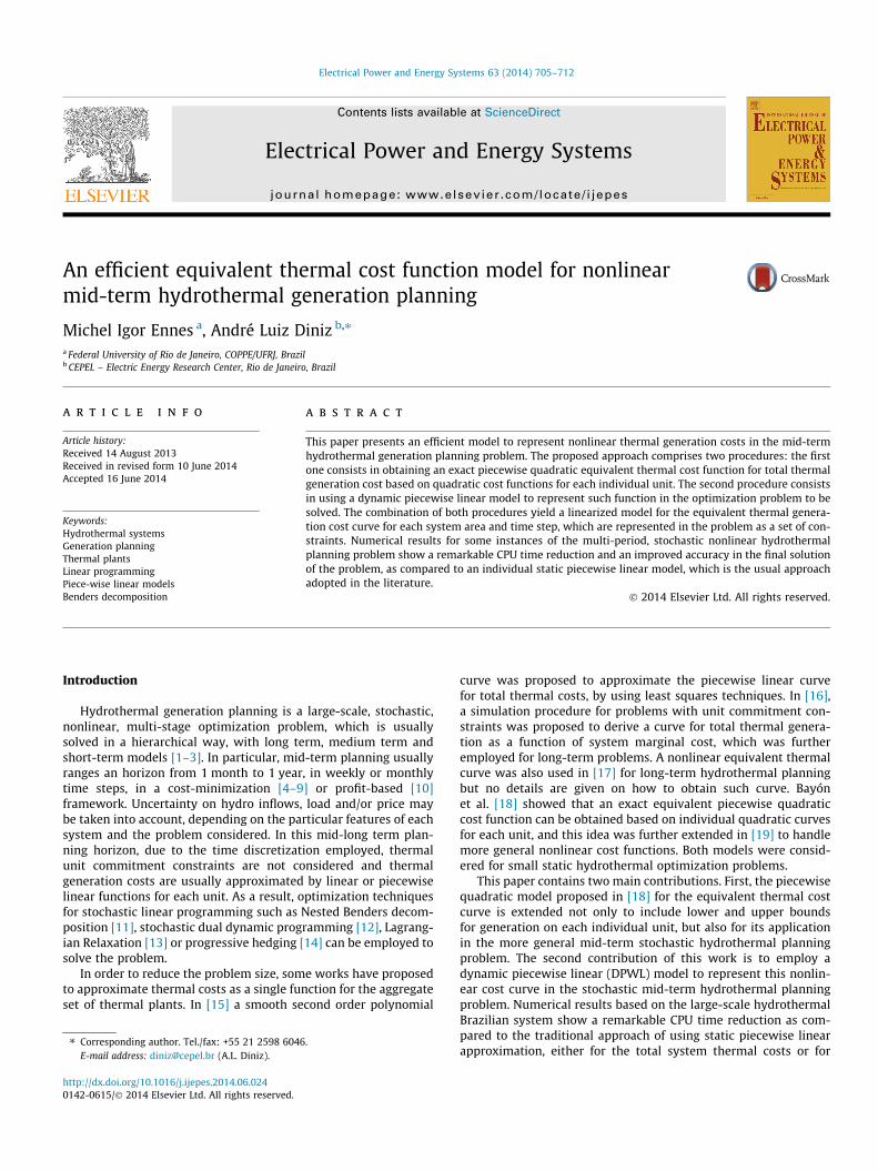
The MTHTS problem is a multi-stage stochastic programmingproblem where the aim is to minimize thermal generation costs,which leads to an optimization of hydro resources in order todispatch the units in an efficient way regarding use of water.Uncertainties on hydro inflows It;x

i to reservoirs are representedby a scenario tree as shown in Fig. 1. In such tree, we denote as(t, x) the node related to time step t and scenario x. The numberof scenarios up to time step t is X(t), so that the total number ofmultistage scenarios is X(T).

Traditional formulation with individual thermal units

The usual formulation of the problem – with individual costfunctions for each thermal unit is shown in (1a)–(1d).

minXT

t¼1

XXðtÞx¼1

pt;xXNT

j¼1

ðc2jðgtt;x

j Þ2 þ c1j

gtt;xj þ c0jÞ

" #

þXXðTÞx¼1

pt;xaðET;xÞ ð1aÞ

s.t.Xj2Ps

gtt;xj þ

Xi2Us

ght;xi þ

Xl2Cs

Inttl;s ¼ Dt

s 8 s; t;x ð1bÞ

ω =1 ω =2 ω =3

...

ω =St = 1 t = 2 t = 3 t = 4 … t = T

Fig. 1. Representation of uncertainties as a scenario tree.

Eti þ GHt

i þ Spti ¼ Et�1

i þ Iti 8 i; t; ð1cÞ

Bounds on E; gh; gt; Int ð1dÞ

The objective function (1a) comprises the sum of total thermalcosts throughout all T time steps and corresponding scenarios,each one with a given probability pt,x. Thermal costs for unit jare given by a second order polynomial function of generation gt,with coefficients c2j, c1j and c0j. At the end of the planning horizonwe consider a so called future cost function a(�) in order to reflectfuture system costs as a function of the vector of end energy sto-rages E in the reservoirs.

The two main constraints of the problem are (1b) and (1c). Eq.(1b) is the energy balance equation: for each system area s, powerdemand Dt;x

s should be met by the sum of hydro and thermal gen-erations in the sets Us and Ps, respectively, of hydro/thermal plantsbelonging to this area. Possible mismatches are allowed by usingavailable energy interchanges Intt

l;s in neighbourhood systems inthe set Cs. If necessary, energy shortages can be included as artifi-cial thermal plants with high incremental costs. Eq. (1c) is theenergy balance in the reservoirs for each time step/scenario. Sincein this paper we are mostly concerned in the representation of thethermal mix, the set of hydro plants are approximated as equiva-lent energy reservoirs based on the formulations described in[21,22]. Variables Et;x

i , ght;xi Spt;x

i denote energy storage, generationand spillage for each equivalent reservoir i. Finally, all variables ofthe problem have proper lower and upper bounds, as stated in(1d).

Alternative formulation with equivalent thermal plants

In mid and long term problems, network constraints are usuallyneglected and transmission is represented only by major inter-change lines. For this reason, it is not so important where eachpower plant is located within each system area. As a consequence,thermal generation costs can be considered by a so-called equiva-lent cost function (ECF), for the total thermal generation in eachsystem area. This is a generalization, to a multi-area setting, ofthe concepts presented in [18] where a single plant for the wholesystem was considered.

According to constraints (1b), total thermal generationGTt

S ¼P

j2psgtj in each system area and each time step depends

on the vector gh of hydro generation values and Int of interchangesamong areas. Moreover, the optimal distribution of this total ther-mal generation among all thermal units in the area is uniquelydefined by the so called coordination equations, which are mathe-matically formulated as follows (see [23], chapter 3).

dcgtj

dgtjðgtjÞ ¼ k; if gtj < gtj < gtj

dcgtj

dgtjðgtjÞP k; if gtj ¼ gtj

dcgtj

dgtjðgtjÞ 6 k; if gtj ¼ gtj

8>>>>><>>>>>:

ð2Þ

where k is the system marginal cost for the corresponding area (wehave suppressed area, time step and scenario indices for simplicityof notation). Constraints (2) correspond to the equal incrementalcost property for the units which are not binding at the optimalsolution (the so called ‘‘marginal units’’).

Based on condition (2) and on the strongly convex property ofthe objective function (provided that all second order terms c2 ofthe cost functions are greater than zero), each value of total areageneration GTt

S is related to a unique area marginal cost k, as wellas a unique optimal solution gt�j ðkÞ for each unit j e Ps. In thissense, the MTHTS can be reformulated by using equivalent thermalplants instead of individual thermal units, as highlighted in expres-sions (3a)–(3e) below. In this new formulation, each equivalent

M.I. Ennes, A.L. Diniz / Electrical Power and Energy Systems 63 (2014) 705–712 707

thermal plant GTts corresponds to the set of all thermal units con-

tained in system area s, as shown in Eq. (3d). The sum of individualthermal costs was also replaced in the objective function by theequivalent thermal cost curve, whose construction is described insection ‘Piecewise quadratic model for equivalent thermal costfunction’.

minXT

t¼1

XXðtÞx¼1

pt;xXNS

s¼1

cGTs ðGTtsÞ

" #þXXðTÞx¼1

pt;xaðET;xÞ ð3aÞ

s.t.

GTts þXi2Us

ght;xi þ

Xl2Cs

Inttl;s ¼ Dt

s 8 s; t;x ð3bÞ

Eti þ GHt

i þ Spti ¼ Et�1

i þ Iti 8 i; t ð3cÞ

GTts ¼

Xj2ps

gttj 8 t; s ð3dÞ

Bounds on E; gh; GT; Int ð3eÞ

In this paper, we considered two solving strategies for problem(1): by performing a multi-stage Benders decomposition approach(MSBD) [11] or by solving the equivalent deterministic formulationof the problem as a big linear program.

Piecewise quadratic model for equivalent thermal cost function

The construction of the equivalent thermal cost function (ECF)takes into account the equal incremental cost property of Eq. (2).If individual generations cost functions are convex, the equivalentgeneration cost function is also convex. In particular, it can beshown that when the individual functions are linear (quadratic),the equivalent function is a piecewise linear (piecewise quadratic)curve [18]. A brief description of the steps to build the ECF for thelatter case, which is the one considered in the paper, is given in thissection. A more detailed explanation with a numerical example ispresented in [24].

Determination of lower and upper bounds

The first step is to determine the lower and upper bounds fortotal thermal generation (x axis) and total generation costs (y axis),which will be given by expressions (4) and (5):

GTs ¼Xj2ps

gtj; GTs ¼Xj2ps

gtj ð4Þ

cGTs ¼Xj2ps

cgtjðgtjÞ; cgts

¼Xj2ps

cgtjðgtjÞ ð5Þ

Partition of the function domain

In this step the domain of the function is divided in severaldisjoint segments [gtsegi

; gtsegi] according to the minimum and max-

imum derivatives of the individual cost function of each unit, i.e.,based on the values of the derivatives in its lower and upper gen-eration limits.

Computation of cost coefficients for each segment

Coefficients ak2, ak

1 and ak0 of the kth segment of the piecewise

quadratic function of the ECF are obtained from the individualcoefficients of the quadratic cost functions for all marginal unitsin this segment, by expression (6) below:

ak2 ¼

dk�dk

2ðpk�pkÞ

ak1 ¼ dk � 2ak

2pk

ak0 ¼ Ck � ak

1pk � ak2ðpkÞ

2

8>>><>>>:

ð6Þ

where pk and pk are the minimum and maximum total thermalgeneration for the segment k, and dk and dk are the derivatives ofthe ECF at the beginning and at the end of the same segment k.The resulting overall cost function cGT(�) is given by:

cGTðGTÞ ¼cGTsegk

ðGTÞ ¼ ak2GT2 þ ak

1GT þ ak0;

for segment k such that GTsegi6 GT 6 GTsegi

8<: ð7Þ

Determination of the generation of each unit

The generation GT�s for the whole set of thermal plant in eacharea s is obtained by solving the MTHTS problem by using an ECFfor each area. Power generation levels for each individual thermalunit is the point where the derivatives of the individual curvematch the marginal cost for its corresponding area, except forthe cases where the minimum (maximum) derivative is greater(lower) than the area marginal costs, where the unit is operatingat its lower (upper) bound. We note that the lower and upperbounds for the generation of each unit have been properly takeninto account both in the power generation values as well as inthe derivatives of the aggregated model (see sections ‘Determina-tion of lower and upper bounds’ and ‘Partition of the functiondomain’). As a consequence, we ensure that those limits are fullyrespected in the final generation values obtained for each unit.

Dynamic piecewise linear approximation of the equivalentcurve

The consideration of the overall thermal generation in each areain a direct way in the optimization problem to be solved wouldlead to a nonlinear stochastic optimization problem. Previousapproaches to consider nonlinear objective function and/orconstraints on stochastic problems have been proposed in the liter-ature, such as generalized Benders decomposition [25], progressivehedging [14] and sequential quadratic programming [26]. How-ever, such solving strategies for nonlinear stochastic programsare not so well established in the literature as compared to sto-chastic linear programming approaches [27]. For this reason, webelieve that it is interesting to formulate the problem as a stochas-tic linear program. The straightforward approach, usually adoptedin the literature and presented in section ‘Static piecewise linear(SPWL) model’, is to employ a piecewise linear model for nonlinearconstraints. In this paper we propose the use of a dynamic piece-wise linear model, as described in section ‘Proposed dynamicpiecewise linear model’.

Static piecewise linear (SPWL) model

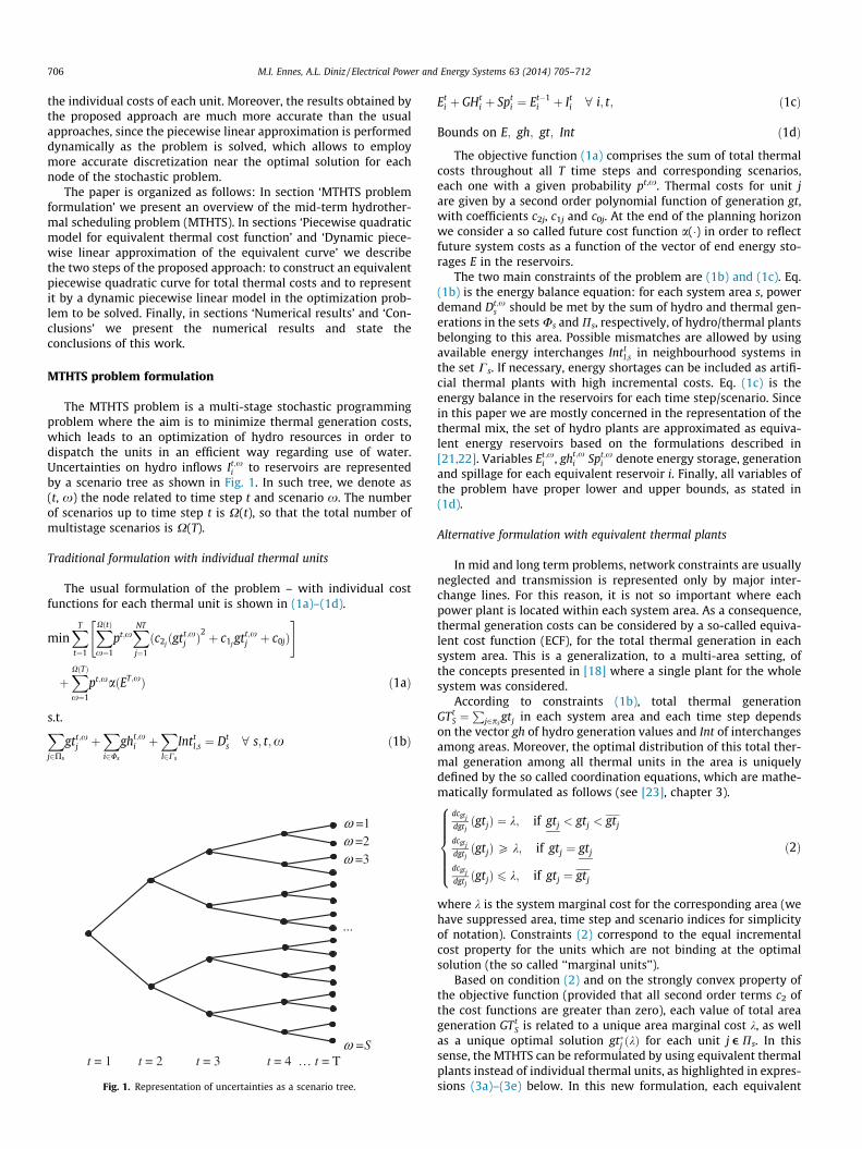
In the so-called static piecewise linear approach (SPWL), weperform an outer approximation of the ECF based on a set of valuesin the x-axis defined a priori, as shown in Fig. 2. The number ofbreakpoints depends on the desired accuracy both for the differ-ences between the exact nonlinear curve and the SPWL modeland for the precision in the thermal generation values.

Proposed dynamic piecewise linear model

The main drawback of the SPWL approach is that a large num-ber of breakpoint is necessary in order to have a high precision

Cgt

GT

Fig. 2. Example of a static piecewise linear model (SPWL) to approximate the ECFfor thermal generation.

708 M.I. Ennes, A.L. Diniz / Electrical Power and Energy Systems 63 (2014) 705–712

model, which would lead to a large linear programming problem.Alternatively, a dynamic piecewise linear approach can be used,where linear approximations are performed only when (andwhere) needed.

Two of the most employed iterative methods to consider non-linear constraints in linear programs are the well know Kelley’scutting plane method [28] and successive linear programming[29]. Based on the successful results reported in [20,30,31] tomodel nonlinear constraints in deterministic problems, we pro-pose an extension, for the case of a nonlinear objective functionand a stochastic program, of the dynamic piecewise linear models(DPWL) proposed in those papers.

The general idea of this strategy is to solve the linear programrelated to the MTHTS problem (or each stage subproblem if aNested Benders decomposition is employed) in a iterative way,adding new cuts to refine the piecewise linear model of the ECFnear to the optimal solution found in the previous iteration. In thisway, it is possible to find a solution as close as desired to the exactnonlinear function. A key feature of this strategy is that it providesa good accuracy not only for function evaluation (cGTs variables),but also for the precision in the thermal generation itself (GTs),with a moderate number of cuts.

Algorithm descriptionWe describe the general steps of the proposed DPWL algorithm

to model the ECF of a specific system area in a given node (t, x). Forthe sake of simplicity, indices t, x are omitted in the sequel and weconsidered the case where the problem is solved as a single linearprogram, with no stage decomposition.

Step 1 – we solve the MTHTS problem, with the current (or ini-tial) piecewise linear model for the ECF. An equivalent thermalgeneration value GT�s is obtained.Step 2 – computation of the exact cost related to GT�s which isgiven by the 2nd degree polynomial cGTsegk

ðGT�s Þ for the kthsegment of the equivalent model where value GT�s is located.Step 3a – we check whether the distance between the cost pro-vided by the piecewise linear model built so far and the exactnonlinear curve is less than a predetermined tolerance dy:

ckGTsðGT�s Þ � cDPWLðGT�s Þ

�� �� 6 dy ð8Þ

If condition (8) is not satisfied, the algorithm jumps to step 4.Otherwise, the precision in the GT�s value is checked against a giventolerance dx in Step 3b.

Step 3b – the GT�s value is associated to either only one active cut(Fig. 3a) or in the intersection of two active cuts (Fig. 3b) of theECF in the current solution found in step 1. We compute dis-tances D1 and D2 between GT�s and points where the active(s)cut(s) intercept the left and right adjacent cuts, respectively.

If both conditions D1 6 dx and D2 6 dx are satisfied, the iterativeprocess for the corresponding node (t, s) stops. Otherwise, the algo-rithm follows to step 4 in order to include new cuts in the model.

Step 4 – independent of the number of active cuts in step 3,NCUTadd new cuts are added in the model, according to a setof points {pi, i = 1 . . . ,NCUTadd} uniformly distributed in theinterval ½GT�s � D1;GT�s þ D2�. Each new cut i is given by the 1storder Taylor approximation at point pi of expression (2) forthe corresponding segment of the piecewise quadratic ECF:

ciDPWLs

ðGTsÞ ¼ dki;sGTs þ RHSk

i;s;

where dki;s ¼

dckGTs

dGTs GTs ¼ pi

���� ¼ 2ak2pi þ ak

1

and RHSki;s ¼ ck

GTsðGT�s Þ � dk

i;spi

8>>>><>>>>:

ð9Þ

Go to step 1.

Overall iterative processThe iterative process described above is performed simulta-

neously for all nodes (t, x) and for the ECF function of all systemareas s. In this sense, the overall process only stops when both dy

and dx tolerances are reached for all combinations of t, x and s.In the case Nested Benders decomposition [11] is employed, theoverall problem is solved by a sequence of forward and backwardpasses, where each node subproblem is solved many times, in dif-ferent outer Benders iterations. In this setting, the iterative processfor each ECF continues normally from the solution of the previousBenders iteration, but tolerances dy and dx may vary along the pro-cess, being tighter as the overall solving procedure evolves. Theoverall iterative procedure stops when both Benders optimalitycriteria and the desired accuracy in the approximation of the ECFare reached.

Special case – linear thermal cost functions

In some decentralized systems, the generation dispatch may beperformed based on price � quantity curves, leading to linear orpiecewise linear thermal generation costs related to bids of thecorresponding utilities. Although this is a particular case of a qua-dratic cost function with c2 = 0, the extension of the approach tosuch case is not trivial and requires the following additionalprocedures:

� In the mixed case (i.e., some thermal plants with linear costsand others with quadratic costs), one thermal plant with linearcost leads to a segment (as defined in Section ‘Partition of thefunction domain’) that contains only this plant. Other plantsthat have not reached its maximum derivative (see [24],Fig. 1) remain in ‘‘stand-by’’ mode until the plant with linearcost has been fully dispatched.� When new points are selected in step 4 of the DPWL procedure,

we verify if the angular coefficient of its corresponding cut isnot the same as any previously added cut in the model of theECF, otherwise it will not be added;

In the numerical results of section ‘Special case - linear thermalcost functions’ we show that even in the pure case (i.e., all thermalcost functions are linear), where the ECF can be represented

Δ1 Δ2

CGTD

C

BA

Active cut

ΔΔ

A

D

C

B

Active cuts

Δ1 Δ2

CGTD

C

BA

Activecut

Δ2Δ1

CGT

Activecuts

*sGT

*sGTGTs GTs

Fig. 3. Active cuts of the DPWL model at each iteration of the proposed algorithm.

M.I. Ennes, A.L. Diniz / Electrical Power and Energy Systems 63 (2014) 705–712 709

exactly as a piecewise linear function in the linear program (2), it isadvantageous to apply the proposed DPWL approach as comparedto the usual SPWL model.

Remarks

The use of an equivalent thermal cost function has somedifficulties in the following cases:

� For the dynamic economic dispatch problem, since rampconstraints may not allow units to operate at an arbitrary regionbetween their lower and upper bounds.� In the thermal unit commitment problem, since we do not

know in advance which units will be on at each time step. Asimulation procedure for the unit commitment problem basedon unit availability and maintenance data is proposed in [16]to estimate the ECF in this case.� When the electrical network is represented, since the sequence

for the dispatch of the thermal units may not follow strictly anincreasing order of marginal costs, due to potential transmis-sion limits that may prevent cheaper units to be dispatchedprior to more expensive units.

However, the aspects mentioned above are intrinsic to shorterterm planning horizons, whereas in this paper we address themid term planning problem. In such longer time horizon, ramplimits and unit commitment constraints are not required and it isnot common to represent the electrical network in detail [1–8].

Table 1Performance comparison between individual (UNIT) and equivalent (EQV) model forthermal costs – DPWL strategy with the problem solved by LP.

Test case UNIT EQV

Optimal cost (103 $) t (s) Optimal cost (103 $) t (s)

S-13 64,539.86072 1.38 64,539.85334 1.33M-13 130,521.57929 4.75 130,521.57100 1.84L-13 260,398.94505 16.9 260398.93492 5.78S-23 164,955.15690 2.45 164,955.15705 1.36M-23 334,265.96026 10.48 334,265.96062 2.19L-23 671,136.62154 70.84 671,136.61864 4.94S-43 232,368.64795 3.75 232,368.64740 1.12M-43 472,885.20921 23.03 472,885.21255 1.91L-43 953,900.21006 221.41 953,900.21125 4.75

Numerical results

Nine different test cases were performed by combining threedifferent thermal configurations (with 13, 23 and 43 units) andthree alternative scenario trees of increasing size: small (2 periodsand 20 scenarios), medium (4 periods and 64 scenarios), and large(8 periods and 128 scenarios). Hydro plants were represented asequivalent reservoirs, as in [22]. We considered three differentcombinations of thermal plants representation and solving strat-egy for the ECF:

� EQV_DPWL: equivalent thermal plant representation (3) withthe proposed dynamic piecewise linear model of section ‘Pro-posed dynamic piecewise linear model’. This is the approachproposed in this paper.� UNIT_DPWL: formulation with individual thermal units (1),

with the proposed DPWL model.� EQV_SPWL: equivalent thermal plant representation (3) with a

static piecewise linear model (section ‘Static piecewise linear(SPWL) model’).

Tolerances dx and dy were set to 0.01%, with NCUTinit =NCUTadd = 4. Two alternative strategies were considered to solveeach problem: either as a single (and big) linear program (LP) orby applying the multi-stage Benders decomposition (MSBD). Opti-mality tolerance e was set to 10�8% in both methods.

Comparisons of the proposed EQV_DPWL approach withUNIT_DPWL and EQV_SPWL models aim to evaluate the advanta-ges of the use of an ECF (section ‘Advantages of the equivalentthermal generation model’) and the DPWL approach (section‘Advantages of the proposed DPWL approach’), respectively, tomodel thermal costs in the MTHTS problem. In sections ‘Perfor-mance of the model regarding the input parameters’ and ‘Feasibil-ity regarding units’ generation bounds’ we assess the performanceand accuracy of the model and in section ‘Accuracy of the finalsolution’ we show the advantages obtained by using the proposedDPWL model even for the linear case.

Advantages of the equivalent thermal generation model

In this subsection we show the advantages of the proposedequivalent model (EQV) as compared to the standard individualmodel (UNIT) for thermal generation costs. In Tables 1 and 2 weshow the results for the LP and MSBD solving strategies, respec-tively. As expected, optimal costs are practically the same, withsmall differences due to tolerances dx and dy for accuracy in ther-mal costs. However, CPU time is much smaller in the proposedequivalent approach, specially for the largest cases.

Advantages of the proposed DPWL approach

We compare the proposed DPWL approach with the standardSPWL model, when an ECF is used for thermal costs. Tables 3 and4 show the results for the MSBD and LP solving strategies,respectively.

Table 2Performance comparison between individual (UNIT) and equivalent (EQV) model for thermal costs – DPWL strategy with the problem solved by MSBD.

Test case UNIT EQV

Optimal cost (103 $) t (s) Niter Optimal cost (103 $) t (s) Niter

S-13 64,539.86137 4.75 2 64,539.86135 5.00 9M-13 130,521.58159 131.25 18 130,521.58148 80.28 16L-13 260,398.94809 716.62 31 260,398.94795 406.79 28S-23 164,955.15769 28.78 10 164,955.15768 14.14 10M-23 334,265.96196 130.92 16 334,265.96194 66.94 15L-23 671,136.62504 1175.97 32 671,136.62271 257.28 26S-43 232,368.65187 8.95 3 232,368.65178 4.41 2M-43 472,885.21707 166.40 14 472,885.21702 55.06 12L-43 953,900.22124 1358.67 33 953,900.22096 331.46 26

Table 3Performance comparison between SPWL and DPWL approaches for the ECF – LPsolving strategy.

Test case SPWL DPWL

Optimal cost (103 $) t (s) Optimal cost (103 $) t (s)

S-13 64,539.85842 0.39 64,539.85334 1.33M-13 130,521.57551 2.09 130,521.57100 1.84L-13 260,398.92487 13.66 260,398.93492 5.78S-23 164,955.15619 0.33 164,955.15705 1.36M-23 334,265.95632 2.03 334,265.96062 2.19L-23 671,136.61060 12.23 671,136.61864 4.94S-43 232,368.64804 0.38 232,368.64740 1.12M-43 472,885.21053 1.98 472,885.21255 1.91L-43 953,900.18845 10.87 953,900.21125 4.75

Table 5Sensitivity analysis of EQV_DPWL approach regarding tolerances for the approxima-tion in the ECF – MSBD solving strategy.

dx, dy (%) Cost (103 $) t (s) Niter

10.00000 953,853.99878 169.42 201.00000 953,898.82541 224.37 260.10000 953,900.20786 249.54 230.01000 953,900.22096 331.46 260.00100 953,900.22126 368.74 310.00010 953,900.22126 408.44 340.00001 953,900.22126 775.15 99a

a There was no convergence in this case, because it has reached the maximumnumber of iterations of the PDD resolution strategy.

Table 6Sensitivity analysis of EQV_DPWL approach regarding input parameter for the initialnumber of cuts.

NCUTinit Cost (103 $) t (s) Niter

4 953900,22096 346,18 268 953900,22114 384,88 3016 953900,22107 372,97 3024 953900,22111 278,07 2640 953900,22111 359,94 28

Table 7Sensitivity analysis of EQV_DPWL approach regarding input parameter for theadditional number of cuts.

3

710 M.I. Ennes, A.L. Diniz / Electrical Power and Energy Systems 63 (2014) 705–712

As in the previous section, optimal costs were nearly the samein both situations, but CPU times were always smaller in the DPWLapproach for the MSBD solving strategy. In the LP strategy, CPUtimes of the DPWL approach are much lower for the larger cases.Even though the usual SPWL approach yielded CPU times lowerfor some of the smaller cases, absolute values are very low. Never-theless, CPU time of the dynamic approach is on average lower ascompared to the static case.

We note that relative CPU times between the two approachesare very dependent on the values of the dx and dy tolerances (seesection ‘Performance of the model regarding the input parame-ters’). If a very high precision is desired for such tolerances, thecpu time of the DPWL method tends to be much smaller than theSPWL approach even for the smaller cases. We carried out an addi-tional run of the S-13 case with a tolerance fifty times lower andobtained CPU times of 1.11 and 6.06 s for the DPWL and SPWLapproaches, respectively.

NCUTadd Cost (10 $) t (s) Niter

2 953900,2210238618 372,65 274 953900,2209632581 367,79 266 953900,2211291293 358,13 298 953900,2211693721 304,37 2710 953900,2211814345 338,24 30

Performance of the model regarding the input parameters

We show in Table 5 a sensitivity analysis on the cost of the opti-mal solution, CPU time and convergence of the proposed

Table 4Performance comparison between SPWL and DPWL approaches for the ECF – MSBD solving strategy.

Test case SPWL DPWL

Optimal cost (103 $) t (s) Niter Optimal cost (103 $) t (s) Niter

S-13 64,539.86133 12.95 2 64,539.86135 5.00 9M-13 130,521.58152 132.59 16 130,521.58148 80.28 16L-13 260,398.94784 715.03 28 260,398.94795 406.79 28S-23 164,955.15767 22.38 10 164,955.15768 14.14 10M-23 334,265.96185 115.84 13 334,265.96194 66.94 15L-23 671,136.62488 690.28 27 671,136.62271 257.28 26S-43 232,368.65184 12.94 2 232,368.65178 4.41 2M-43 472,885.21693 105.50 11 472,885.21702 55.06 12L-43 953,900.22105 653.95 25 953,900.22096 331.46 26

gtnorm (%)

Fig. 4. Feasibility check for the set of all thermal generation levels, regarding itslower and upper bounds.

Table 8Differences in power outputs for thermal units between UNIT and EQV approaches.

All cases/all deviations Deviations for case G-13

Case Average difference in poweroutput (MW)

Unit # Average difference in poweroutput (MW)

S-13 9.40191e�06 6 0.0014420L-13 1.64674e�04 7 0.0004268S-23 4.89539e�05 8 0.0013870L-23 1.10197e�04 9 0.0005949S-43 4.16883e�05 10 0.0002083L-43 5.94556e�05 Other

unitsZero

Average distance (MW)

Case G-13 – unit # 6

Fig. 5. Worst case cumulative distribution of differences between power outputvalues of UNIT and EQV approaches.

M.I. Ennes, A.L. Diniz / Electrical Power and Energy Systems 63 (2014) 705–712 711

EQV_DPWL regarding the values of tolerances dx and dy for thelargest case (L-43) solved by MSBD.

As expected, the cost increases as tolerances are lower, since theECF becomes progressively more refined. However, cost differencesare very low for tolerance values smaller than 0.01%. Therefore,there are no substantial gains when using tolerances beyond thisthreshold, since the decrease in the optimal cost is around10�10%, with a noticeable increase in CPU time.

In Tables 6 and 7 we show a sensitivity analysis on the numberof initial and additional cuts for the same L-43 case. Since there areno significant differences in the performance among the differentcombination for these parameters, we conclude that theEQV_DPWL approach is sufficiently robust for a wide range of val-ues for these parameters.

We note that, since we use an optimization-based solving strat-egy and the overall problem is convex, the values shown fromTables 4–7 correspond to the global optimal solution for a givenapproximation of the true nonlinear thermal cost function. How-ever, since Table 5 shows that this optimal value does not chanceas the tolerance in this approximation reaches values 100 timeslower than 0.001%, we conclude that we have been sufficientlyclose to the optimal value of the nonlinear optimization problem.

1 We recall that once having obtained the optimal solution for the problem withthe EQV_DPWL model, generations per unit can be computed as described in section‘Determination of the generation of each unit’.

Feasibility regarding units generation bounds

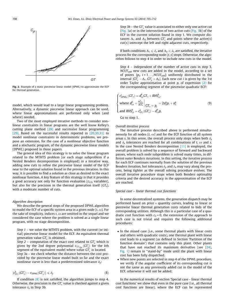
This section shows that, despite having used an aggregatemodel for the thermal generation, all individual lower and upperbounds have been respected in the final solution obtained by ourmodel, due to expressions (4) and (5). Fig. 4 shows the distributionof thermal generation levels comprising all thermal units and alltime steps for the largest case (L-43). Each dot represents the nor-malized value gtnorm for the thermal generation of a thermal unit j

at a given scenario x of time step t, computed as a percentagevalue of the range between its lower and upper bounds, accordingto (10). It can be seen that all generations values are within theirfeasible range, due to the lack of negative values and/or valuesgreater than 100%.

gtt;xnormj

¼ 100�gtt;x

j � gtj

gtj � gtj

ð10Þ

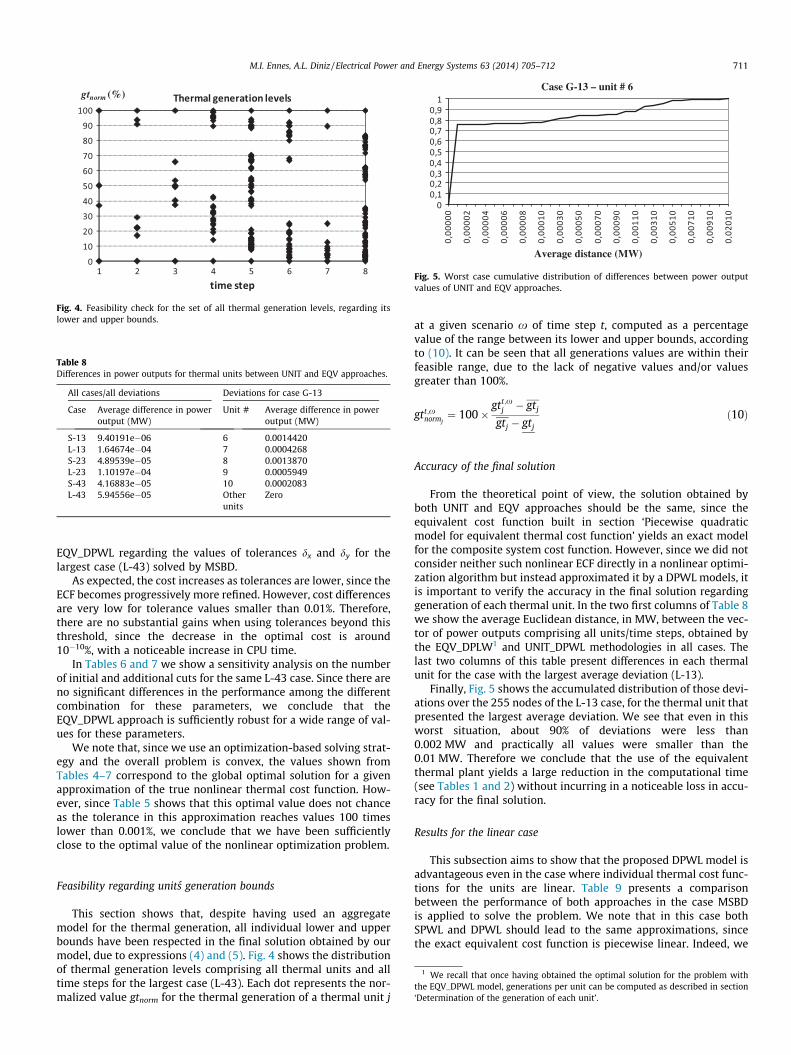
Accuracy of the final solution

From the theoretical point of view, the solution obtained byboth UNIT and EQV approaches should be the same, since theequivalent cost function built in section ‘Piecewise quadraticmodel for equivalent thermal cost function’ yields an exact modelfor the composite system cost function. However, since we did notconsider neither such nonlinear ECF directly in a nonlinear optimi-zation algorithm but instead approximated it by a DPWL models, itis important to verify the accuracy in the final solution regardinggeneration of each thermal unit. In the two first columns of Table 8we show the average Euclidean distance, in MW, between the vec-tor of power outputs comprising all units/time steps, obtained bythe EQV_DPLW1 and UNIT_DPWL methodologies in all cases. Thelast two columns of this table present differences in each thermalunit for the case with the largest average deviation (L-13).

Finally, Fig. 5 shows the accumulated distribution of those devi-ations over the 255 nodes of the L-13 case, for the thermal unit thatpresented the largest average deviation. We see that even in thisworst situation, about 90% of deviations were less than0.002 MW and practically all values were smaller than the0.01 MW. Therefore we conclude that the use of the equivalentthermal plant yields a large reduction in the computational time(see Tables 1 and 2) without incurring in a noticeable loss in accu-racy for the final solution.

Results for the linear case

This subsection aims to show that the proposed DPWL model isadvantageous even in the case where individual thermal cost func-tions for the units are linear. Table 9 presents a comparisonbetween the performance of both approaches in the case MSBDis applied to solve the problem. We note that in this case bothSPWL and DPWL should lead to the same approximations, sincethe exact equivalent cost function is piecewise linear. Indeed, we

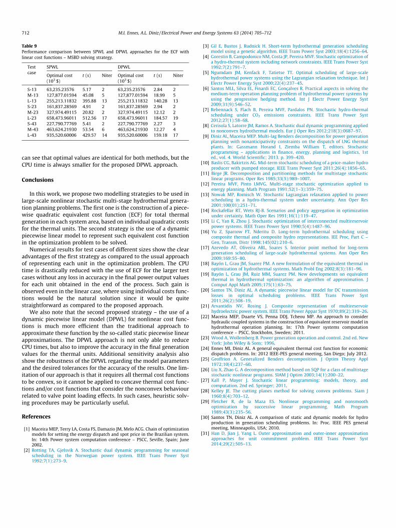
Table 9Performance comparison between SPWL and DPWL approaches for the ECF withlinear cost functions – MSBD solving strategy.

Testcase

SPWL DPWL

Optimal cost(103 $)

t (s) Niter Optimal cost(103 $)

t (s) Niter

S-13 63,235.23576 5.17 2 63,235.23576 2.84 2M-13 127,877.01594 45.08 5 127,877.01594 18.99 5L-13 255,213.11832 395.88 13 255,213.11832 140.28 13S-23 161,837.28569 4.91 2 161,837.28569 2.94 2M-23 327,974.49115 20.82 2 327,974.49115 12.12 2L-23 658,473.96011 512.56 17 658,473.96011 184.57 19S-43 227,790.77769 5.41 2 227,790.77769 2.27 3M-43 463,624.21930 53.54 6 463,624.21930 12.27 4L-43 935,520.60006 429.57 14 935,520.60006 159.18 17

712 M.I. Ennes, A.L. Diniz / Electrical Power and Energy Systems 63 (2014) 705–712

can see that optimal values are identical for both methods, but theCPU time is always smaller for the proposed DPWL approach.

Conclusions

In this work, we propose two modelling strategies to be used inlarge-scale nonlinear stochastic multi-stage hydrothermal genera-tion planning problems. The first one is the construction of a piece-wise quadratic equivalent cost function (ECF) for total thermalgeneration in each system area, based on individual quadratic costsfor the thermal units. The second strategy is the use of a dynamicpiecewise linear model to represent such equivalent cost functionin the optimization problem to be solved.

Numerical results for test cases of different sizes show the clearadvantages of the first strategy as compared to the usual approachof representing each unit in the optimization problem. The CPUtime is drastically reduced with the use of ECF for the larger testcases without any loss in accuracy in the final power output valuesfor each unit obtained in the end of the process. Such gain isobserved even in the linear case, where using individual costs func-tions would be the natural solution since it would be quitestraightforward as compared to the proposed approach.

We also note that the second proposed strategy – the use of adynamic piecewise linear model (DPWL) for nonlinear cost func-tions is much more efficient than the traditional approach toapproximate these function by the so-called static piecewise linearapproximations. The DPWL approach is not only able to reduceCPU times, but also to improve the accuracy in the final generationvalues for the thermal units. Additional sensitivity analysis alsoshow the robustness of the DPWL regarding the model parametersand the desired tolerances for the accuracy of the results. One lim-itation of our approach is that it requires all thermal cost functionsto be convex, so it cannot be applied to concave thermal cost func-tions and/or cost functions that consider the nonconvex behaviourrelated to valve point loading effects. In such cases, heuristic solv-ing procedures may be particularly useful.

References

[1] Maceira MEP, Terry LA, Costa FS, Damazio JM, Melo ACG. Chain of optimizationmodels for setting the energy dispatch and spot price in the Brazilian system.In: 14th Power system computation conference – PSCC, Seville, Spain; June2002.

[2] Rotting TA, Gjelsvik A. Stochastic dual dynamic programming for seasonalscheduling in the Norwegian power system. IEEE Trans Power Syst1992;7(1):273–9.

[3] Gil E, Bustos J, Rudnick H. Short-term hydrothermal generation schedulingmodel using a genetic algorithm. IEEE Trans Power Syst 2003;18(4):1256–64.

[4] Gorestin B, Campodonico NM, Costa JP, Pereira MVF. Stochastic optimization ofa hydro-thermal system including network constraints. IEEE Trans Power Syst1992;7(2):791–7.

[5] Ngumdam JM, Kenfack F, Tatietse TT. Optimal scheduling of large-scalehydrothermal power systems using the Lagrangian relaxation technique. Int JElectr Power Energy Syst 2000;22(4):237–45.

[6] Santos MLL, Silva EL, Finardi EC, Gonçalves R. Practical aspects in solving themedium-term operation planning problem of hydrothermal power systems byusing the progressive hedging method. Int J Electr Power Energy Syst2009;31(9):546–52.

[7] Rebennack S, Flach B, Pereira MVF, Pardalos PN. Stochastic hydro-thermalscheduling under CO2 emissions constraints. IEEE Trans Power Syst2012;27(1):58–68.

[8] Cerisola S, Latorre JM, Ramos A. Stochastic dual dynamic programming appliedto nonconvex hydrothermal models. Eur J Oper Res 2012;218(3):0687–97.

[9] Diniz AL, Maceira MEP. Multi-lag Benders decomposition for power generationplanning with nonanticipativity constraints on the dispatch of LNG thermalplants. In: Gassmann Horand I, Ziemba William T, editors. Stochasticprogramming – applications in finance, energy, planning and logistics, 1sted., vol. 4. World Scientific; 2013. p. 399–420.

[10] Baslis CG, Bakirtzis AG. Mid-term stochastic scheduling of a price-maker hydroproducer with pumped storage. IEEE Trans Power Syst 2011;26(4):1856–65.

[11] Birge JR. Decomposition and partitioning methods for multistage stochasticlinear programs. Oper Res 1985;33(5):989–1007.

[12] Pereira MVF, Pinto LMVG. Multi-stage stochastic optimization applied toenergy planning. Math Program 1991;52(1–3):359–75.

[13] Nowak MP, Romisch W. Stochastic Lagrangian relaxation applied to powerscheduling in a hydro-thermal system under uncertainty. Ann Oper Res2001;100(01):251–71.

[14] Rockafellar RT, Wets RJ-B. Scenarios and policy aggregation in optimizationunder certainty. Math Oper Res 1991;16(1):119–47.

[15] Li C, Yan R, Zhou J. Stochastic optimization of interconnected multireservoirpower systems. IEEE Trans Power Syst 1990;5(4):1487–96.

[16] Yu Z, Sparrow FT, Nderitu D. Long-term hydrothermal scheduling usingcomposite thermal and composite hydro representations. IEE Proc, Part C –Gen, Transm, Distr 1998;145(02):210–6.

[17] Azevedo AT, Oliveira ARL, Soares S. Interior point method for long-termgeneration scheduling of large-scale hydrothermal systems. Ann Oper Res2009;169:55–80.

[18] Bayón L, Grau JM, Suarez PM. A new formulation of the equivalent thermal inoptimization of hydrothermal systems. Math Probl Eng 2002;8(3):181–96.

[19] Bayón L, Grau JM, Ruiz MM, Suarez PM. New developments on equivalentthermal in hydrothermal optimization: an algorithm of approximation. JComput Appl Math 2005;175(1):63–75.

[20] Santos TN, Diniz AL. A dynamic piecewise linear model for DC transmissionlosses in optimal scheduling problems. IEEE Trans Power Syst2011;26(2):508–19.

[21] Arvantidis NV, Rosing J. Composite representation of multireservoirhydroelectric power system. IEEE Trans Power Appar Syst 1970;89(2):319–26.

[22] Maceira MEP, Duarte VS, Penna DDJ, Tcheou MP. An approach to considerhydraulic coupled systems in the construction of equivalent reservoir model inhydrothermal operation planning. In: 17th Power systems computationconference – PSCC, Stockholm, Sweden; 2011.

[23] Wood A, Wollemberg B. Power generation operation and control. 2nd ed. NewYork: John Wiley & Sons; 1996.

[24] Ennes MI, Diniz AL. A general equivalent thermal cost function for economicdispatch problems. In: 2012 IEEE-PES general meeting, San Diego; July 2012.

[25] Geoffrion A. Generalized Benders decomposition. J Optim Theory Appl1972;10(4):237–60.

[26] Liu X, Zhao G. A decomposition method based on SQP for a class of multistagestochastic nonlinear programs. SIAM J Optim 2003;14(1):200–22.

[27] Kall P, Mayer J. Stochastic linear programming: models, theory, andcomputation. 2nd ed. Springer; 2011.

[28] Kelley JE. The cutting planes method for solving convex problems. Siam J1960;8(4):703–12.

[29] Fletcher R, de la Maza ES. Nonlinear programming and nonsmoothoptimization by successive linear programming. Math Program1989;43(3):235–56.

[30] Santos TN, Diniz AL. A comparison of static and dynamic models for hydroproduction in generation scheduling problems. In: Proc. IEEE PES generalmeeting, Minneapolis, USA; 2010.

[31] Han D, Jian J, Yang L. Outer approximation and outer-inner approximationapproaches for unit commitment problem. IEEE Trans Power Syst2014;29(2):505–13.