An Effective Architecture and Algorithm for Detecting Worms with

Various Scan Techniques

Jiang Wu, Sarma Vangala, Lixin GaoDepartment of Electrical and Computer Engineering,

University of Massachusetts,Amherst, MA 01002.

Email: (jiawu,svangala,lgao)@ecs.umass.edu

Kevin KwiatAir Force Research Lab,Information Directorate,

525 Brooks Road,Rome, NY 13441.

Email: kwiatk@rl.af.mil

Abstract

Since the days of the Morris worm, the spread ofmalicious code has been the most imminent menace tothe Internet. Worms use various scanning methods tospread rapidly. Worms that select scan destinationscarefully can cause more damage than worms employingrandom scan. This paper analyzes various scan tech-niques. We then propose a generic worm detection ar-chitecture that monitors malicious activities. We pro-pose and evaluate an algorithm to detect the spread ofworms using real time traces and simulations. We findthat our solution can detect worm activities when only4% of the vulnerable machines are infected. Our resultsbring insight on the future battle against worm attacks.

1 Introduction

A worm is a program that propagates across a net-work by exploiting security flaws of machines in the net-work. The key difference between a worm and a virus isthat a worm is autonomous. That is, the spread of ac-tive worms does not need any human interaction. As aresult, active worms can spread in as fast as a few min-utes [7][12]. Recent worms, like Code Red and Slammercost public and private sectors millions of dollars. Fur-

0This work is supported in part by NSF Grant ANI-0208116,the Alfred Sloan Fellowship and the Air Force Research Lab.Any opinions, findings, and conclusions or recommendations ex-pressed in this material are those of the authors and do not nec-essarily reflect the views of the National Science Foundation, theAlfred Sloan Foundation or the Air Force Research Lab.

thermore, the propagation of active worms enables oneto control millions of hosts by launching distributed de-nial of service (DDOS) attacks, accessing confidentialinformation, and destroying/corrupting valuable data.Accurate and prompt detection of active worms is crit-ical for mitigating the impact of worm activities.In this paper, first, we present an analysis on po-

tential scan techniques that worms can employ to scanvulnerable machines. In particular, we find that wormscan choose targets more carefully than the randomscan. A worm that scans only IP addresses announcedin the global routing table can spread faster than aworm that employs random scan. In fact, scan meth-ods of this type have already been used by the Slapperworm[9]. These methods reduce the time wasted onunassigned IP addresses. They are easy to implementand pose the most imminent menace to the Internet.We analyze a family of scan methods and compare themto the random scan. We find that these scan meth-ods can dramatically increase the spreading speed ofworms.Second, we propose a worm detection architecture

and algorithms for prompt detection of worm activities.Our worm detection architecture takes advantage of thefact that a worm typically scans some unassigned IP ad-dresses or an inactive port of assigned IP addresses. Bymonitoring unassigned IP addresses or inactive ports,one can collect statistics on scan traffic. These statis-tics include the number of source/destination addressesand volume of the scan traffic. We propose a detec-tion algorithm called victim number based algorithm,which relies solely on the increase of source addressesof scan traffic and evaluates its effectiveness. We findthat it can detect the Code Red like worm when only

4% of the vulnerable machines are infected.This paper is organized as follows. Section 2 intro-

duces and analyzes various scan methods. By com-paring the spreading speed of various scan methods,we show that routable worms spread the fastest andpose the greatest menace to the Internet. In Section3, a generic worm detection architecture is introduced.Then, the victim number based algorithm is designedand evaluated. Section 4 concludes the paper.

1.1 Related Work

A lot of work has been done in analyzing worms,modeling worm propagation and designing possibleworms. In [18], Weaver designed fast spreading worms,called the Warhol worms, by using various scan meth-ods. In [12], Staniford et. al. systematically introducedthe threats of worms and analyzed well-known worms.In addition, smarter scan methods such as local subnet,hitlist and permutation scans were designed. Instead ofusing the idea of selecting as many assigned addressesas possible, these methods focus on increasing the effi-ciency of the worm scan process itself.Many models were designed to analyze the spread-

ing of worms. Kephart and White designed an epi-demiological model to measure the virus populationdynamics[3]. Zou et. al.[23] designed a two-factorworm model, which takes into consideration the fac-tors that slow the worm propagation. In [20], Chenet. al. designed a concise discrete time model whichcan adapt parameters such as the worm scan rate, thevulnerability patching rate and the victim death rate.By analyzing the factors that influence the spread ofworms, these models and methods give an insight intocontaining worm propagation effectively.More important problems are detection and defense.

As in the fight against computer viruses, accurate de-tection and quick defense are always difficult problemsfor unprecedented attacks. There are a number of de-tection methods using Internet traffic measurementsto detect worms on networks. Zou et.al.[23], exploredthe possibility of monitoring Internet traffic with smallsized address spaces and predicting the worm propaga-tion. Cheung’s activity graph based detection[13] usesthe scan activity graph (the sender and receiver of apacket are the vertices and the relation between themare the edges) inferred from the traffic. This methoduses the fact that the activity graph can be large onlyfor a very short period of time. Spitzner[11] introducedthe idea of Honeypots. Honeypots are hosts that pre-tend to own a number of IP addresses and passivelymonitor packets sent to them. Honeypots can also beused to fight back a worm’s attack. An example is theLaBrea tool[14] designed by Liston, which reduces theworm spreading speed by holding TCP sessions withworm victims for a long time.Methods to detect worms that cause anomalies on a

single computer were also designed. Somayaji and For-

rest’s defense solution[10] uses a system call sequencedatabase and compares new sequences with them. Ifa mismatch is found, then the sequence is delayed.Williamson’s “Virus Throttle”[19] checks if a computersends SYN packets to new addresses. If so, the packetwill be delayed for a short period of time. By delay-ing instead of dropping, these two solutions reduce theimpact of false alarms. This paper proposes detectionmethods that can detect large scale worm attacks onthe Internet or enterprise networks.

2 Scan Methods

Probing is the first thing that worms perform to findvulnerable hosts. Depending on how worms choosetheir scan destinations from a given address space, scanmethods can be classified as random scan, routablescan, hitlist scan and divide-conquer scan. In this sec-tion, we present a set of scan methods and comparetheir spreading speeds.

2.1 Selective Random Scan

Instead of scanning the whole IP address space atrandom, a set of addresses that more likely belong toexisting machines can be selected as the target ad-dress space. The selected address list can be eitherobtained from the global or the local routing tables.We call this kind of scanning selective random scan.Care needs to be taken so that unallocated or reservedaddress blocks in the IP address space are not selectedfor scanning. Worms can avoid using addresses withinthese address blocks. Information about such addressblocks can be found in the following ways. An exampleis the Bogon list[8], which contains around 32 addressblocks. The addresses in these blocks should never ap-pear in the public network. IANA’s IPv4 address allo-cation map[4] is a similar list that shows the /8 addressblocks which have been allocated. The “Slapper”[9](orApache, OpenSSL) worm made use of these lists in or-der to spread rapidly. Worms using the selective ran-dom scan need to carry information about the selectedtarget addresses. Carrying more information enlargesthe worm’s code size and slows down its infection pro-cess. For selective random scan, the database carryingthe information can be hundreds of bytes. Therefore,the additional database will not greatly affect the al-ready slow spreading of worms.

2.1.1 Propagation Speed of Selective Random

Scan

Two current models used are the Weaver’s model in[17] and the AAWP model in [20]. Due to their similarmodeling performance as shown in Figure 1, we adoptthe AAWP worm propagation model[20]. In the AAWPmodel the spread of worm is characterized as follows:

0 200 400 600 800 1000 12000

0.5

1

1.5

2

2.5

3

3.5

4

4.5

5x 10

5

Time

No.

of i

nfec

ted

mac

hine

s

AAWPWeavers model

Figure 1. Comparison of AAWP Model and Weaver’s Simulator for scan rate=100/sec, no. of vulnerablemachines=500,000 and hitlist size=10,000. Note that the curves of the two models overlap.

ni+1 = ni + [N − ni][1− (1−1

T)sni ] (1)

where N is the total number of vulnerable machines; Tis the number of addresses used by the worm as scantargets; s is the scan rate (the number of scan packetssent out by a worm infected host per time tick) and ni

is the number of machines infected up to time tick i.The length of the time tick is determined by the timeneeded to completely infect a machine (denoted by t).These notations are used consistently throughout thispaper.In Equation (1), the first term on the right hand side

denotes the number of infected machines alive at theend of time tick i. The term, N −ni, denotes the num-ber of vulnerable machines not infected by time tick i.The remaining term, 1− (1− 1

T)sni , is the probability

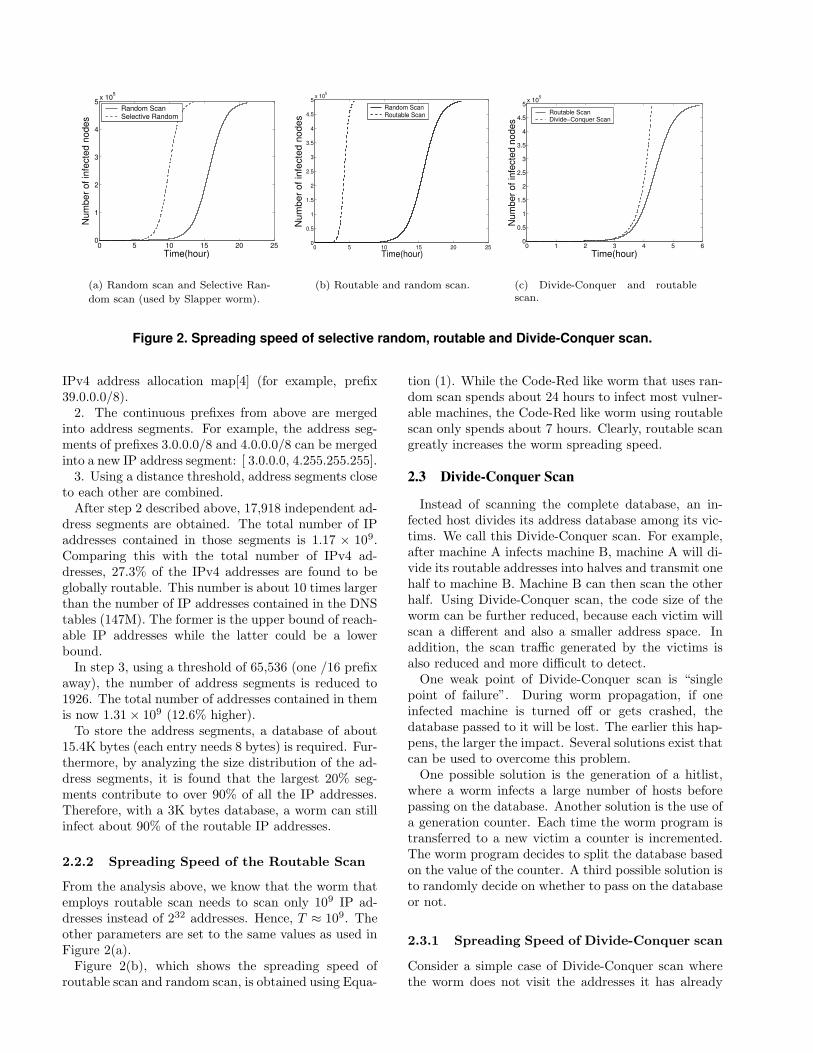
that an uninfected machine will be infected at the endof time tick i + 1. This model is different from [20] inthat the death rate (rate by which infected machinesreset or crash) and the patch rate (rate by which vul-nerable machines are fixed and become invulnerable)are assumed to be zero. This is because our goal is tofind the effect of address space selection on the wormspread.Figure 2(a), obtained from Equation (1), shows the

spreading speed of worms that use random scan and se-lective random scan techniques. The selective randomscan was used by the Slapper worm. Once it infects amachine, the Slapper worm scans only a predefined setof Class A machines[22]. The total number of vulner-able machines (N), the scan rate (s) and t are set to500,000, 2 scans/second and 1 second respectively forboth the random scan and the selective random scan.The Slapper worm which uses selective random scanhas 2.7×109 addresses as scan targets (T ). Figure 2(a)demonstrates that using a target address pool that issmaller than the whole IP address space can speed up

the worm propagation.

2.2 Routable Scan

In addition to the reduced scanning address space, ifa worm also knows which of the addresses are routableor are in use, then it can spread faster and more ef-fectively and can avoid detection. This type of scan-ning technique, where unassigned IP addresses whichare not routable on the Internet are removed from theworm’s database, is called routable scan. One problemwith this type of scan method is that the code size ofthe worm has to be increased as it needs to carry aroutable IP address database. The database cannot betoo large as it leads to a long infection time resultingin a slow down of the worm propagation. In the nextsubsection we design and analyze a possible routablescanning technique.

2.2.1 Design and Analysis of Routable Scan

BGP is the global routing protocol that glues the in-dependent networks together. From the global BGProuting tables, globally routable prefixes can be ob-tained. Some BGP routing tables are also available onthe Internet. This data provides worm designers withmethods that can enhance the performance of worms.To find out the applicability of using a BGP table asthe database, we analyze a typical global BGP routingtable with two objectives. The first is to find how manyprefixes are globally routable. The second is to find theminimum size of the database a worm must carry. Thisanalysis is done in 3 steps:1. The BGP table we used is from one of the Route

Views servers[21]. The routing table contains about112K prefixes. By removing the redundant prefixes,49K independent prefixes were obtained. In addi-tion, those prefixes that are known to be unallocatedwere removed by checking the BGP table with IANA’s

0 5 10 15 20 250

1

2

3

4

5x 10

5

Time(hour)

Num

ber o

f inf

ecte

d no

des

Random ScanSelective Random

(a) Random scan and Selective Ran-

dom scan (used by Slapper worm).

0 5 10 15 20 250

0.5

1

1.5

2

2.5

3

3.5

4

4.5

5x 10

5

Time(hour)

Num

ber

of in

fect

ed n

odes

Random ScanRoutable Scan

(b) Routable and random scan.

0 1 2 3 4 5 60

0.5

1

1.5

2

2.5

3

3.5

4

4.5

5x 10

5

Time(hour)

Num

ber o

f inf

ecte

d no

des

Routable ScanDivide−Conquer Scan

(c) Divide-Conquer and routablescan.

Figure 2. Spreading speed of selective random, routable and Divide-Conquer scan.

IPv4 address allocation map[4] (for example, prefix39.0.0.0/8).2. The continuous prefixes from above are merged

into address segments. For example, the address seg-ments of prefixes 3.0.0.0/8 and 4.0.0.0/8 can be mergedinto a new IP address segment: [ 3.0.0.0, 4.255.255.255].3. Using a distance threshold, address segments close

to each other are combined.After step 2 described above, 17,918 independent ad-

dress segments are obtained. The total number of IPaddresses contained in those segments is 1.17 × 109.Comparing this with the total number of IPv4 ad-dresses, 27.3% of the IPv4 addresses are found to beglobally routable. This number is about 10 times largerthan the number of IP addresses contained in the DNStables (147M). The former is the upper bound of reach-able IP addresses while the latter could be a lowerbound.In step 3, using a threshold of 65,536 (one /16 prefix

away), the number of address segments is reduced to1926. The total number of addresses contained in themis now 1.31× 109 (12.6% higher).To store the address segments, a database of about

15.4K bytes (each entry needs 8 bytes) is required. Fur-thermore, by analyzing the size distribution of the ad-dress segments, it is found that the largest 20% seg-ments contribute to over 90% of all the IP addresses.Therefore, with a 3K bytes database, a worm can stillinfect about 90% of the routable IP addresses.

2.2.2 Spreading Speed of the Routable Scan

From the analysis above, we know that the worm thatemploys routable scan needs to scan only 109 IP ad-dresses instead of 232 addresses. Hence, T ≈ 109. Theother parameters are set to the same values as used inFigure 2(a).Figure 2(b), which shows the spreading speed of

routable scan and random scan, is obtained using Equa-

tion (1). While the Code-Red like worm that uses ran-dom scan spends about 24 hours to infect most vulner-able machines, the Code-Red like worm using routablescan only spends about 7 hours. Clearly, routable scangreatly increases the worm spreading speed.

2.3 Divide-Conquer Scan

Instead of scanning the complete database, an in-fected host divides its address database among its vic-tims. We call this Divide-Conquer scan. For example,after machine A infects machine B, machine A will di-vide its routable addresses into halves and transmit onehalf to machine B. Machine B can then scan the otherhalf. Using Divide-Conquer scan, the code size of theworm can be further reduced, because each victim willscan a different and also a smaller address space. Inaddition, the scan traffic generated by the victims isalso reduced and more difficult to detect.One weak point of Divide-Conquer scan is “single

point of failure”. During worm propagation, if oneinfected machine is turned off or gets crashed, thedatabase passed to it will be lost. The earlier this hap-pens, the larger the impact. Several solutions exist thatcan be used to overcome this problem.One possible solution is the generation of a hitlist,

where a worm infects a large number of hosts beforepassing on the database. Another solution is the use ofa generation counter. Each time the worm program istransferred to a new victim a counter is incremented.The worm program decides to split the database basedon the value of the counter. A third possible solution isto randomly decide on whether to pass on the databaseor not.

2.3.1 Spreading Speed of Divide-Conquer scan

Consider a simple case of Divide-Conquer scan wherethe worm does not visit the addresses it has already

visited. This reduces the probing range. We now havethe following spread pattern for the Divide-Conquerscan:

ni+1 = (N−ni)[1− (1−1

109 −∑i−1

j=0 njs)sni ]+ni (2)

where i ≥ 0.Using the same set of parameters used for the

routable scan, Figure 2(c) shows that the Divide-Conquer scan is much faster than the routable scan,although the spreading process is more complicated.Furthermore, for the Divide-Conquer scan, even whenthere are few uninfected vulnerable machines, thespreading speed increases, rather than slowing downunlike the earlier cases.

2.4 Hybrid Scan

Limiting the scan targets by a specific addressdatabase might miss many vulnerable hosts that arenot globally reachable. To solve this problem, the at-tacker can combine routable scan with random scan ata later stage of the propagation (when most addresseshave been scanned) to infect more machines. This typeof scanning technique is called Hybrid scan. The ad-vantage of this technique is that even though the prop-agation has been detected, the hybrid scan can be usedto infect more number of machines as it is already toolate for effective defense.Considering the fact that a large number of machines

use private IP addresses and are hidden and protectedby gateway machines from the Internet, better per-formance can be achieved if those addresses can bescanned with more power. In addition, each networkinterface card of a victim could be used for the wormscan to reach more subnets.

2.5 Extreme Scan Methods

In this section, we introduce and analyze several ex-treme scan methods. We call them “extreme” becausethe worms need to use some brute-force techniques tocreate a scan target address database. Because theworm scans only the hosts contained in the database,it can avoid from being detected. On the other hand,each method entails some critical limitations. That is,worms using extreme scan methods might spread veryslowly or have weaknesses that can be exploited for de-tection.

2.5.1 DNS Scan

The worm designer could use the IP addresses obtainedfrom DNS servers to build the target address database.Its advantage is that the gathered IP addresses are al-most always definitely in use. However, it also has someproblems. First, it is not easy to get the complete list

of addresses that have DNS records. Second, the num-ber of addresses is limited to those machines having apublic domain name. From the observations of DavidMoore[6], we know that about half of the victims ofCode Red I did not have DNS records. Third, becausethe worm programs need to carry a very large addressdatabase, the worms will spread very slowly.Using the AAWP model, DNS scan’s spreading speed

can be analyzed. Here, T ≈ 108. We assume the infec-tion time t is roughly proportional to the worm’s codesize due to the transmission time. We use Code-Red Iv2 as the standard, which has a code size of 5K bytes.Other parameters in Equation (1) are the same as usedbefore. Figure 3(a) shows that DNS worm spread canbarely start because of the huge address database theworm must carry.

2.5.2 Complete Scan

This is the most extreme method a worm designermight use to prevent the worm scan from being de-tected. The worm designer can use some method toget the complete list of assigned IP addresses and usethe list as the target address database. Then, it is hardfor a monitor to distinguish the malicious scans fromthe legitimate ones. The Flash Worm introduced byStaniford[12] is similar to this type of worm.Using this method, the size of the attacker’s code will

also be very large because a large address list has to becarried with the code. From our former analysis, thenumber of distinct host addresses should be more than100 million. Without compression, the list size will beat least 400M bytes, which will greatly slow down theinfection time. However, for a specific vulnerability, thelist could be reduced to a reasonable size. For exam-ple, if the objective of the attack is a security hole onrouters, the attacker could collect a list of routers. Asthe number of routers on the Internet is much smaller,a complete scan will be applicable.Using the same method and parameters used for the

DNS scan, we can analyze the performance of com-plete scan. Figure 3(b) shows that when the addressdatabase is larger than 6M bytes and if no databasesplitting is used, the Code Red like worm using com-plete scan will spread slower than the one using randomscan. We introduce a small death rate of 0.002% anda patch rate of 0.0002% in this case to clearly differ-entiate the various cases of complete scan. Besides thecode size and the death rate, the remaining parame-ters are the ones used to simulate the Code Red worm.The infection rate graph, therefore, does not rise to themaximum possible value of 500,000.

2.6 Comparison of the Worm Scan Methods

The basic difference between the various scan meth-ods lies in the selection of the address database. If thecode size is large and the average bandwidth possessed

0 50 100 150 2000

1

2

3

4

5x 10

5

Time(hour)

Num

ber

of in

fect

ed n

odes

Random ScanDNS Scan

(a) DNS scan and random scan.

0 5 10 15 20 25 300

1

2

3

4

5x 10

5

Time(hour)

Num

ber

of in

fect

ed n

odes

RandomComplete(1M list)Complete(2M list)Complete(6M list)

(b) Complete scan and randomscan.

0 5 10 15 20 25 300

0.5

1

1.5

2

2.5

3

3.5

4

4.5

5x 10

5

Time(hour)

Num

ber o

f inf

ecte

d no

des

RandomSelective RandomRoutableComplete(1M list)Complete(2M list)Complete(6M list)

(c) Comparison of scan methods.

Figure 3. Extreme scan methods and comparison of major scan methods

by the infected host is given, then the time taken bya worm to infect a host is roughly determined by thespeed of transmission of a copy of the worm program.Hence, we can see that the better the granularity of thedatabase, the stealthier the scan technique. However,the size of the worm program will inevitably increase.There exists a tradeoff between the size of the addressdatabase and the speed of the worm spread. Figure3(c) shows this tradeoff. Besides the list size and thedeath rate as in the case of the complete scan, otherparameters in this figure are still the ones used to sim-ulate the Code Red worm.We can see that when the worm scan uses a better

address database, similar to routable scan, the proba-bility that a vulnerable machine gets infected is larger.For selective random scan and routable scan, the spreadis faster than in the random scan. However, for a wormusing complete scan, when the database size is largerthan 1M bytes, the worm will spread slower than aworm using routable scan. A 1M bytes database canbe translated to a list containing around 250K vulnera-ble hosts, which is not very large considering the num-ber of Code Red victims. When the size of the list islarger than 6M bytes, the worm using complete scanwill spread even slower than the worm using randomscan. Although a worm using complete scan can ef-fectively avoid being detected, the size of the addressdatabase cannot be too large. We can also see thatslower spread will reduce the total number of victimsthe worm can infect.We do not include Divide-Conquer scan here because

we are trying find scan methods that are easy to im-plement. Considering the average power of the ma-chines that can be used by the worm, we find that, aworm could use routable scan first and random scanlater when most of the routable addresses have beeninfected. This combination does not cost much andleverages benefits from different scan methods.

3 Worm Detection

The main focus of this section is to detect worms us-ing various scan techniques. Worm scan detection israising an alarm upon sensing anomalies that are mostlikely caused by large scale worm spreads. Our goalis to quickly detect unknown worms on large enter-prise networks or the Internet while making the falsealarm probability as low as possible. In the followingsections, we first present our generic worm detectionarchitecture. We then present the design and analysisof a simple detection algorithm, called, victim numberbased algorithm.

3.1 Generic Worm Detection Architecture

To detect worms, we need to analyze Internet traffic.Monitoring traffic towards a single network is often notenough to find a worm attack. The traffic pattern couldappear normal during a worm attack because the wormhas not yet infected the network or will not infect it atall. Therefore, we have to monitor the network behav-ior at as many places as possible in order to reduce thechance of false alarms.To achieve this, we need a distributed detection archi-

tecture. The architecture monitors the network behav-ior at different places. By gathering information fromdifferent networks, the detection center can determinethe presence of a large scale worm attack. Problemssuch as where the monitors should be deployed, whichaddresses need to be monitored and how the detectionsystem works need to be considered in designing thedetection architecture.We propose a generic traffic monitoring and worm

detection architecture, as shown in Figure 4. The archi-tecture is composed of a control center and a number ofdetection components. To reduce noise, traffic towardsinactive addresses is preferred to be used for worm de-tection. The detection components will pre-analyze thetraffic and send preliminary results or alarms to the

control center. The control center collects reports fromthe detection components and makes the final decisionon whether there is anything serious happening.

3.1.1 Implementation of Detection Compo-

nents

The detection components can be deployed in one ofthe following two places.

1. Monitors In Local Networks: The detection com-ponents can be implemented on virtual machinesor on the gateways of local networks.

2. Traffic Analyzers Beside Routers: Detection com-ponents can also be traffic analyzers beside therouters, observing the traffic of a set of addresses.Because of the processing costs associated withthis form of detection, the analyzers cannot usecomplicated filtering rules. For example, they mayonly watch traffic sent towards unallocated /8 net-works instead of particular addresses or they mayjust count the traffic volume.

3.1.2 Address Space Selection

The detection network consists of addresses monitoredby detection components. Although a large detectionnetwork is highly desirable, the number of addresses thesystem can manage is limited. New worms might notscan the whole IP address space. In addition, differ-ent worms might use different target spaces. To makepacket collection efficient and effective, we need to de-ploy the detection components so that the detectionnetwork overlaps as much as possible with the wormscan target space.For the random scan, detection components can be

deployed anywhere. For the routable scan or theDivide-Conquer scan, deploying detection componentsfor allocated IP address spaces is better. Therefore, todetect worms that may be using any of the three scanmethods, it would be better to use the latter strategy.To collect inactive addresses, IP address blocks that

are not assigned or known to be inactive for appli-cations (for example most dial-up users do not haveHTTP servers) are used. For the attackers using a ran-dom set of such address blocks, it will be difficult toknow the detection network. Some virtual machinescould also be setup to respond to the scan packets theyreceive. Hence, the attacker will not be able to tellthe difference between inactive addresses and active ad-dresses.

3.2 Victim Number Based Algorithm

Using the detection architecture, we need to designalgorithms to detect anomalies caused by worms. Sincea new worm’s signature is not known beforehand, asmall number of packets is not enough to detect the

worm. It is abnormal to find a large amount of scantraffic sent towards inactive addresses. This is, how-ever, prone to false alarms because the scan traffic canbe caused by other reasons (such as DDOS and soft-ware errors). Therefore, it is necessary to find someunique and common characteristics of worms.Serious worm incidents usually involve a large num-

ber of hosts that scan specific ports on a set of ad-dresses. Many of these addresses are inactive. If wedetect a large number of distinct addresses scanningthe inactive ports, within a short period of time, thenit is highly possible that a worm attack is going on. Wedefine the addresses from which a packet is sent to aninactive address as victims. If the detection system cantrack the number of victims, then the detection systemhas a better performance. Hence, a good decision ruleto determine if a host is a victim is necessary.

3.2.1 Victim Decision Rules

To decide if a host is a victim, the simplest decisionrule is that at least one scan packet is received by aninactive host. We call this the “One Scan DecisionRule” (OSDR). Using this rule, the number of victimsdetected by the detection system over a period of timecan be modelled as:

Vk =

k∑

i=0

[ni − ni−1][1− (1−D/T )(k−i)s] (3)

where Vk is the number of victims detected by the sys-tem up to time tick k (here the death rate and patchrate are both assumed to be zero and n

−1 = 0) andD is the detection network size. In [20], Chen et. al.proved that for an address space containing more than220 addresses, the number of victims determined by thedetection system closely matches the dynamics of therandom scan’s propagation.Though simple, OSDR is susceptible to daily scan

noise. Any host that has a scan packet collected by thedetection network is considered to be a victim. DavidMoore’s work[6] showed that “two scans captured bythe host leads to a victim”. This “Two Scan DecisionRule” (TSDR) works well with noise and reflects theincessant feature of worm scans. We focus on TSDR inthis paper.TSDR reduces most of the sporadic scans caused

by port scans or software errors. Apparently, higherthe number of scan packets used to make the decision,higher is the decision accuracy. Yet this allows morevictims to slip away from the detection system. Thenumber of victims detected by a detection system us-ing TSDR up to time tick k can be calculated by theequation:

Local Network

Detecting Component

Local Network

Local Network

Detecting Component

Monitoring and detection center

Detecting Component

Internet or Large Enterprise Network

Routers

Data Transfer

Figure 4. A generic traffic monitoring and worm detection architecture.

Vk =k

∑

i=0

[ni−ni−1][1−ρ(k−i)s

−ρ(k−i)s−1(1−ρ)(k−i)s]

(4)where the number of infected hosts up to time tick i isni and ρ = (1−

DT). Here, we assume the death rate and

patch rate to be zero and n−1 = 0. On the right hand

side of the equation, ni − ni−1, is the number of newlyinfected machines during time tick i. The total numberof machines detected at the end of time tick k is thesum of machines detected at every time tick i before k.ρ(k−i)s denotes the fraction of victims infected duringtime tick i but were never detected up to time tick k.The term ρ(k−i)s−1(1 − ρ)(k − i) denotes the fractionof victims infected during time tick i but only one oftheir scan packets has been detected by time tick k.Equations (3) and (4) above are based on the as-

sumption that each new victim will use the same ad-dress space as the destination address space used bythe worm. This is a common feature of the two scanmethods presented earlier. We also assume that theaddress space used for detection is always a subset ofthe address space used by the worm. The death rateand the patch rate are ignored.For the Divide-Conquer scan, each victim will scan

the addresses only within its piece of the target space.Therefore, the fraction of victims captured by the de-tection system is the fraction of address space that thedetection system covers. If we assume that the victimsare randomly distributed around the address space usedby the attacker, and s ≥ 1, then the number of victimsdetected by time tick k can be expressed by a muchsimpler equation:

Vk =D

Tnk−1 (5)

3.2.2 Detection Threshold

The victim number based algorithm consists of threeparts: First, all scan packets with inactive destination

addresses are gathered. This task is accomplished bythe detection architecture. Second, the victims are re-trieved from the gathered addresses. This has beendiscussed in the previous subsection. Third, an adap-tive threshold is needed to determine when a surge islarge enough. During the monitoring of blocks of inac-tive addresses, if there is a quick surge in the numberof distinct victims, then there is an evidence of a seri-ous worm attack. The victim number based detectionalgorithm is based on the above principle.Using only inactive addresses, the noise caused by

normal scan traffic and other attacks can be reduced.This method requires simple filtering rules to gathersuspicious packets and count them. Hence, it is veryfast. The following facts can also be used in orderto demonstrate the effectiveness of our solution. Portscans are usually done by a limited number of hosts andnormal DOS or DDOS traffic will not focus on inactiveaddresses. Hence, these will not cause much impact onour solution.To combat noise that might be received by the archi-

tecture, the scan volume is kept stable. This allows usto use an adaptive threshold that can help in detect-ing abnormality. If there is deviation in the number ofvictims obtained within a certain period of time, thenthe victim number based algorithm’s threshold shouldbe able to reflect it. The threshold could be expressedby:

Ti = γ ∗

√

√

√

√

1

k

i−1∑

j=i−k

(Vj − E[Vi])2 = γ ∗ σ (6)

E[Vi] =1

k

i−1∑

j=i−k

Vj (7)

where Ti is the threshold to be used by the system attime tick i; γ is a constant value called threshold ratio;Vj is the number of new victims detected during eachk time ticks starting from i − k time ticks; k is thelearning time of the system, which is the time takenby the system to calculate E[Vi]; E[Vi] is the rate of

increase in the number of new victims at every timetick i averaged over the k time ticks. If the rate ofincrease of victims detected during the ith time tick isgreater than the threshold value set during that time,then there is abnormality present in the system. Inpractice, we also need to find continuous number ofsuch abnormalities to determine worm activity. Thenumber of continuous abnormalities needed to detectworm activity is denoted as r. A tradeoff is necessaryin selecting the value of r. A large value of r givea better detection performance but take longer timewhereas a smaller value might result in false positivesbut take lesser time.Initially, the number of new victims detected is large

as there are only a small number of addresses in thedatabase. This leads to a large rate of increase showingpeaks in the detection curve. However, as the databasegets larger and larger the rate of increase of new victimsobserved decreases. In order to smooth these peaks ofthe initial learning process, we need to have some wayfor entries to expire in the database. A simple methodis to use new databases everyday. For a specific day,the learning process will start from what the databaselearned from the previous day.Another method is to assign a decreasing life time

L to each new victim detected. If L decreases to zerothen the victim is considered dead and removed fromthe victim list. If a scan packet is received from thevictim before L expires, its life time is then reset to L.Using this method, the size of the database can be keptstable. However, tracking the time for each address isexpensive. We use the first method for our solution.Another static threshold that reflects a maximum

possible victim number observed by the system overa period can also be used. Whenever this thresholdis reached, an alarm is raised regardless of the formerself-learning threshold.It needs to be pointed out that when the worm scan

level is comparable to the normal noise level, the wormwill not be detected. Therefore, the system will usuallyraise an alarm only when it detects large scale wormattacks. We set the parameters γ, r and k using thetechnique shown in Appendix B.

3.3 Traffic Trace Used To Validate The Algorithm

Once the parameters γ, r and k are appropriately se-lected (Appendix B), we need to test the solution withreal traffic traces obtained from worm incidents in orderto validate the detection method. However, it is verydifficult to find such Internet traffic traces which arepublicly available. As background traffic, we use Inter-net traffic traces from the WAND research group[16].The traffic traces are gathered from the gateways onthe campus network at University of Auckland, NewZealand, who own a /16 prefix. Using worm infec-tion dynamics obtained from the AAWP model andEquation (4), we simulate the number of worm victims

8 9 10 11 12 13 14 15 160

2000

4000

6000

8000

10000

12000

Detection network size (/#)

Det

ectio

n tim

e (s

econ

ds)

N=500K, s=10N=500K, s=25N=500K, s=50N=500K, s=100N=1.25M, s=10N=2.5M, s=10N=5M, s=10

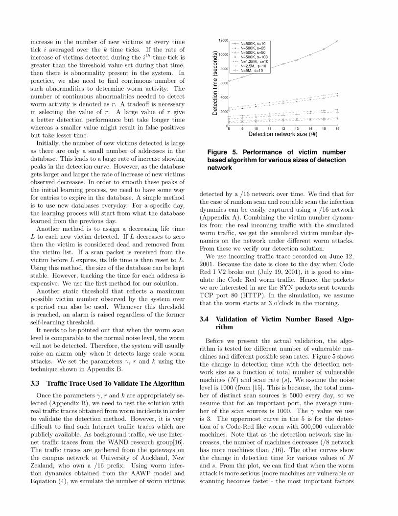
Figure 5. Performance of victim numberbased algorithm for various sizes of detectionnetwork

detected by a /16 network over time. We find that forthe case of random scan and routable scan the infectiondynamics can be easily captured using a /16 network(Appendix A). Combining the victim number dynam-ics from the real incoming traffic with the simulatedworm traffic, we get the simulated victim number dy-namics on the network under different worm attacks.From these we verify our detection solution.We use incoming traffic trace recorded on June 12,

2001. Because the date is close to the day when CodeRed I V2 broke out (July 19, 2001), it is good to sim-ulate the Code Red worm traffic. Hence, the packetswe are interested in are the SYN packets sent towardsTCP port 80 (HTTP). In the simulation, we assumethat the worm starts at 3 o’clock in the morning.

3.4 Validation of Victim Number Based Algo-rithm

Before we present the actual validation, the algo-rithm is tested for different number of vulnerable ma-chines and different possible scan rates. Figure 5 showsthe change in detection time with the detection net-work size as a function of total number of vulnerablemachines (N) and scan rate (s). We assume the noiselevel is 1000 (from [15]. This is because, the total num-ber of distinct scan sources is 5000 every day, so weassume that for an important port, the average num-ber of the scan sources is 1000. The γ value we useis 3. The uppermost curve in the 5 is for the detec-tion of a Code-Red like worm with 500,000 vulnerablemachines. Note that as the detection network size in-creases, the number of machines decreases (/8 networkhas more machines than /16). The other curves showthe change in detection time for various values of Nand s. From the plot, we can find that when the wormattack is more serious (more machines are vulnerable orscanning becomes faster - the most important factors

0 5 10 15 20 2510

0

101

102

103

Incr

ease

rat

e of

dis

tinct

sou

rces

Time (hour)

Normal trafficPlus random scan traffic

Detected at 13:48< 2% infected

Worm starts spread at 3:00

(a) Variation of victim number in case of randomscan

0 5 10 15 20 2510

0

101

102

103

104

Incr

ease

rat

e of

dis

tinct

sou

rces

Time (hour)

Normal trafficPlus routable scan traffic

Detected at 6:05<1.1% infected

Worm starts spread at 3:00

(b) Variation of victim number in case of routablescan

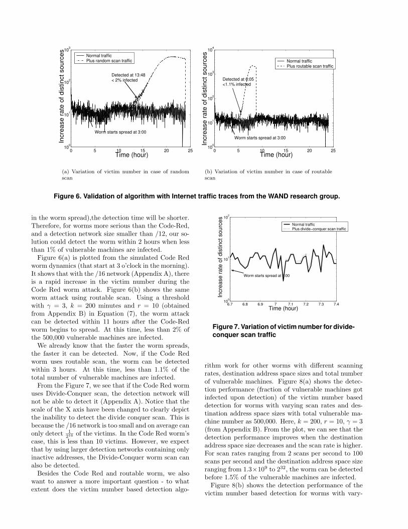
Figure 6. Validation of algorithm with Internet traffic traces from the WAND research group.

in the worm spread),the detection time will be shorter.Therefore, for worms more serious than the Code-Red,and a detection network size smaller than /12, our so-lution could detect the worm within 2 hours when lessthan 1% of vulnerable machines are infected.Figure 6(a) is plotted from the simulated Code Red

worm dynamics (that start at 3 o’clock in the morning).It shows that with the /16 network (Appendix A), thereis a rapid increase in the victim number during theCode Red worm attack. Figure 6(b) shows the sameworm attack using routable scan. Using a thresholdwith γ = 3, k = 200 minutes and r = 10 (obtainedfrom Appendix B) in Equation (7), the worm attackcan be detected within 11 hours after the Code-Redworm begins to spread. At this time, less than 2% ofthe 500,000 vulnerable machines are infected.We already know that the faster the worm spreads,

the faster it can be detected. Now, if the Code Redworm uses routable scan, the worm can be detectedwithin 3 hours. At this time, less than 1.1% of thetotal number of vulnerable machines are infected.From the Figure 7, we see that if the Code Red worm

uses Divide-Conquer scan, the detection network willnot be able to detect it (Appendix A). Notice that thescale of the X axis have been changed to clearly depictthe inability to detect the divide conquer scan. This isbecause the /16 network is too small and on average canonly detect 1

216 of the victims. In the Code Red worm’scase, this is less than 10 victims. However, we expectthat by using larger detection networks containing onlyinactive addresses, the Divide-Conquer worm scan canalso be detected.Besides the Code Red and routable worm, we also

want to answer a more important question - to whatextent does the victim number based detection algo-

6.7 6.8 6.9 7 7.1 7.2 7.3 7.410

0

101

102

Incr

ease

rate

of d

istin

ct s

ourc

es

Time (hour)

Normal trafficPlus divide−conquer scan traffic

Worm starts spread at 3:00

Figure 7. Variation of victim number for divide-conquer scan traffic

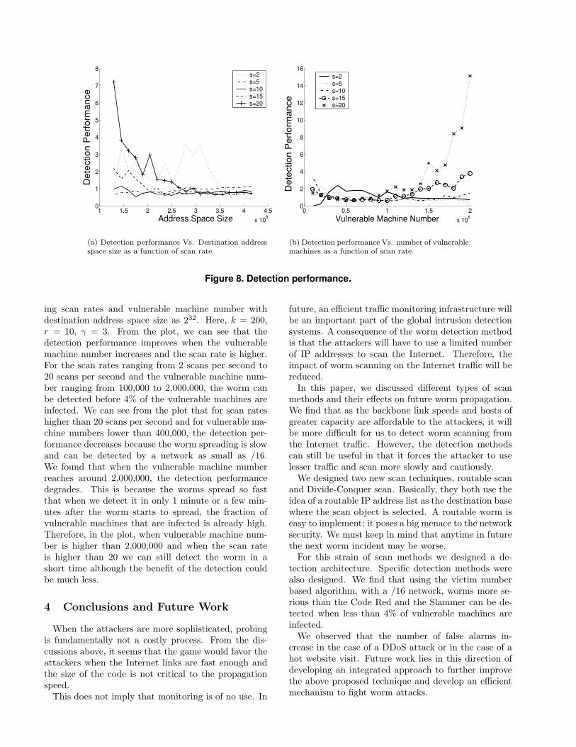
rithm work for other worms with different scanningrates, destination address space sizes and total numberof vulnerable machines. Figure 8(a) shows the detec-tion performance (fraction of vulnerable machines gotinfected upon detection) of the victim number baseddetection for worms with varying scan rates and des-tination address space sizes with total vulnerable ma-chine number as 500,000. Here, k = 200, r = 10, γ = 3(from Appendix B). From the plot, we can see that thedetection performance improves when the destinationaddress space size decreases and the scan rate is higher.For scan rates ranging from 2 scans per second to 100scans per second and the destination address space sizeranging from 1.3×109 to 232, the worm can be detectedbefore 1.5% of the vulnerable machines are infected.Figure 8(b) shows the detection performance of the

victim number based detection for worms with vary-

1 1.5 2 2.5 3 3.5 4 4.5x 10

9

0

1

2

3

4

5

6

7

8

Det

ectio

n P

erfo

rman

ce

Address Space Size

s=2s=5s=10s=15s=20

(a) Detection performance Vs. Destination addressspace size as a function of scan rate.

0 0.5 1 1.5 2x 10

6

0

2

4

6

8

10

12

14

16

Det

ectio

n P

erfo

rman

ce

Vulnerable Machine Number

s=2s=5s=10s=15s=20

(b) Detection performance Vs. number of vulnerablemachines as a function of scan rate.

Figure 8. Detection performance.

ing scan rates and vulnerable machine number withdestination address space size as 232. Here, k = 200,r = 10, γ = 3. From the plot, we can see that thedetection performance improves when the vulnerablemachine number increases and the scan rate is higher.For the scan rates ranging from 2 scans per second to20 scans per second and the vulnerable machine num-ber ranging from 100,000 to 2,000,000, the worm canbe detected before 4% of the vulnerable machines areinfected. We can see from the plot that for scan rateshigher than 20 scans per second and for vulnerable ma-chine numbers lower than 400,000, the detection per-formance decreases because the worm spreading is slowand can be detected by a network as small as /16.We found that when the vulnerable machine numberreaches around 2,000,000, the detection performancedegrades. This is because the worms spread so fastthat when we detect it in only 1 minute or a few min-utes after the worm starts to spread, the fraction ofvulnerable machines that are infected is already high.Therefore, in the plot, when vulnerable machine num-ber is higher than 2,000,000 and when the scan rateis higher than 20 we can still detect the worm in ashort time although the benefit of the detection couldbe much less.

4 Conclusions and Future Work

When the attackers are more sophisticated, probingis fundamentally not a costly process. From the dis-cussions above, it seems that the game would favor theattackers when the Internet links are fast enough andthe size of the code is not critical to the propagationspeed.This does not imply that monitoring is of no use. In

future, an efficient traffic monitoring infrastructure willbe an important part of the global intrusion detectionsystems. A consequence of the worm detection methodis that the attackers will have to use a limited numberof IP addresses to scan the Internet. Therefore, theimpact of worm scanning on the Internet traffic will bereduced.In this paper, we discussed different types of scan

methods and their effects on future worm propagation.We find that as the backbone link speeds and hosts ofgreater capacity are affordable to the attackers, it willbe more difficult for us to detect worm scanning fromthe Internet traffic. However, the detection methodscan still be useful in that it forces the attacker to uselesser traffic and scan more slowly and cautiously.We designed two new scan techniques, routable scan

and Divide-Conquer scan. Basically, they both use theidea of a routable IP address list as the destination basewhere the scan object is selected. A routable worm iseasy to implement; it poses a big menace to the networksecurity. We must keep in mind that anytime in futurethe next worm incident may be worse.For this strain of scan methods we designed a de-

tection architecture. Specific detection methods werealso designed. We find that using the victim numberbased algorithm, with a /16 network, worms more se-rious than the Code Red and the Slammer can be de-tected when less than 4% of vulnerable machines areinfected.We observed that the number of false alarms in-

crease in the case of a DDoS attack or in the case of ahot website visit. Future work lies in this direction ofdeveloping an integrated approach to further improvethe above proposed technique and develop an efficientmechanism to fight worm attacks.

References

[1] D. Moore, The Spread of the Code-Red Worm(CRV2), http://www.caida.org/analysis/ secu-rity/ code-red/coderedv2/analysis.xml

[2] Fyodor, The Art of Port Scanning, http://www.insecure.org, Sept. 1997

[3] J. O. Kephart and S. R. White. Measuring andModeling Computer Virus P revalence, Proc. ofthe 1993 IEEE Computer Society Symposium onResearch in Security and Privacy, 2-15, May. 1993,

[4] Internet Protocol V4 Address Space,http://www.iana.org/assignments/ipv4-address-space/

[5] T. Liston. LaBrea, http://www.hackbusters.net/LaBrea/

[6] D. Moore. Code-Red: A Case Study on theSpread and Victims of an Internet Worm,http://www.icir.org /vern/imw-2002/imw2002-papers/209.ps.gz

[7] D. Moore, V. Paxson, S. Savage, C. Shannon,S. Staniford and N. Weaver The Spread of theSapphire/Slammer Worm http://www.caida.org/outreach/papers/2003/ sapphire/sapphire.html

[8] R. Thomas, Bogon List v1.5 07 Aug 2002http://www.cymru.com/Documents/bogon-list.html

[9] Internet Storm Center, OpenSSL Vulnerabilities,http://isc.incidents.org/analysis.html?id=167,Sept. 2002,

[10] A. Somayaji, S. Forrest, Automated Response Us-ing System-Call Delays, Proceedings of 9th UsenixSecurity Symposium, Denver, Colorado 2000.

[11] L. Spitzner, Strategies and Issues:Honeypots - Sticking It to Hackershttp://www.networkmagazine.com/article/NMG20030403S0005

[12] S. Staniford, V. Paxson and N. Weaver. Howto 0wn the Internet in Your Spare Time,http://www.icir.org/vern/papers/cdc-usenix-sec02/

[13] S. Cheung. Graph-based Intrusion Detec-tion System (GrIDS) http://seclab.cs.ucdavis.edu/arpa/grids/PI meeting (Savannah).pdf,Jan. 1999

[14] T. Liston, Welcome To My Tarpit - The Tacti-cal and Strategic Use of LaBrea, http://www.hackbusters.net/

[15] V. Yegneswaran, P. Barford and J. Ullrich Inter-net Intrusions: Global Characteristics and Preva-lence, SIGMETRICS 2003.

[16] Waikato Internet Traffic Storage, http://wand.cs.waikato.ac.nz/wand/wits/index.html

[17] Warhol Worms: The potentialfor Very Fast Internet Plagues,http://www.cs.berkeley.edu/ nweaver/warhol.html

[18] N. Weaver, Potential Strategies for HighSpeed Active Worms: A Worst Case Analysis,http://www.cs.berkeley.edu/∼nweaver/worms.pdf

[19] M. M. Williamson, Throttling Viruses: Restrict-ing Propagation to Defeat Malicious Mobile Code,http://www.hpl.hp.com/techreports/2002/HPL-2002-172.pdf

[20] Z. Chen, L. Gao and K. Kwiat, Modeling theSpread of Active Worms, IEEE INFOCOM 2003

[21] University of Oregon Route Views Project,http://www.routeviews.org

[22] Global Slapper Worm Information Center,http://www.f-secure.com/v-descs/slapper.shtml

[23] C. Zou, L. Gao, W. Gong and D. Towsley, Mon-itoring and Early Warning for Internet Worms,Umass ECE Technical Report TR-CSE-03-01,2003.

5 Appendices

A Impact of Network Size on Observed

Number of Victims

As our solution uses only the inactive addresses, itapplies to worms that blindly probe an address space.This is because they do not know which hosts are vul-nerable beforehand. This is a reasonable assumption,otherwise a worm that knows the list of vulnerablehosts, could just infect them one by one. In this case,the weak worm scan traffic can go completely unde-tected. An ideal detection system should with a rea-sonable sized detection network be able to detect largescale worm propagation soon after the victim numberbecomes much larger than the normal scan noise level.Using the formulas derived earlier, we can analyze

the performance of our solution for worms using dif-ferent scan methods. We define performance as theleast size of detection network needed to ensure that aworm is detected within a certain time. Intuitively, thelarger the detection network, the faster will the numberof victims detected approaches the real victim numberand thus exceeds the threshold. Below are the evalu-ations for worms using several scan methods. We useTSDR in order to detect scanning for each of the scanmethods.

0 5 10 15 20 250

1

2

3

4

5 x 105

Time(hour)

Num

ber o

f vic

tims

Routable Scan victimsDetected by /8 networkDetected by /12 networkDetected by /16 network

(a) Random Scan.

0 1 2 3 4 5 60

0.5

1

1.5

2

2.5

3

3.5

4

4.5

5x 10

5

Time(hour)

Num

ber o

f vic

tims

Routable Scan victimsDetected victims by /8 networkDetected victims by /12 networkDetected victims by /16 network

(b) Routable scan.

0 1 2 3 4 50

1

2

3

4

5 x 105

Time(hour)

Num

ber o

f vic

tims

Divide Conquer Scan victimsDetected with /8 networkDetected with /6 networkDetected with /4 network

(c) Divide-Conquer scan.

Figure 9. Impact of detection network size on observed number of victims

1. Random Scan: Figure 9(a) shows the detectioncurve of for random scan. We see that the detec-tion curve approaches the infection curve when thedetection network size is over 220 (a /12 network).

2. Routable Scan: For routable scan, Equation (4)can be used to simulate the detection curve. FromFigure 9(b), we see that the detection curve alsocatches up closely with the infection curve whenthe detection network size is over 220.

3. Divide-Conquer Scan: From Figure 9(c), we cansee that even when a /4 detection network is usedfor Divide-Conquer scan, the detection curve stilllags far behind the infection curve (in the /4 case,the fraction of victims that could be detected isless than 1/16). This means that Divide-Conquerscan is difficult to detect.

From above, we can observe that infection dynamicsof the first two scan methods can be captured with sameperformance. The Divide-Conquer scan is very hard todetect as only a fixed fraction of victims can be de-tected. This is because random scan and routable scanvictims share the same target address space while theDivide-Conquer victims use only a piece of the wholeaddress space. When the detection network size or thevulnerable machine number is too small, our detectionsolution might fail. Fortunately, Divide-Conquer scanhas its limitations and can be combined with randomscan to enhance its performance making our solutionto work in that particular case also.

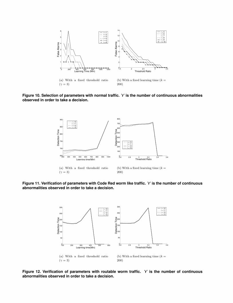
B Selection of Parameters

In selecting parameters for the detection system themost important factor we consider is false alarms. Byapplying our detection system for various parametersettings we were able to choose the parameters withreasonable efficiency. The learning time, k, cannot be

too long as it can lead to a lower detection performanceby making the detection time longer. This can in turnlead to increased number of infections. We choose avalue of 200 minutes for k. We also find that a value ofr ≥ 6 leads to a decreased number of false alarms. Avalue of γ ≥ 3.4 makes worm detection difficult. Fig-ures 10(a), 10(b), 11(a) and 11(b) justify the above as-sumptions. We assume that the June 12th traffic tracedoes not contain major worm attack traffic in obtain-ing the previous plots. Figure 10(a) shows that whenγ = 3, by selecting r ≥ 6 and using a learning timek ≥ 200 minutes, we can eliminate false positives.In Figure 10(b), we can see that even when using

r as large as 10, we still need γ to be larger than 3to eliminate false positives completely. From Figure11(a), we can see that when γ is 3, k is around 200 andr ≥ 10, the detection time is the lowest. One thing wecan observe from 11(b) is that when γ is larger than3.4, the worm cannot be detected.The verification of the above parameters for the

routable scan method is shown in Figures 12(a) and12(b). For the verification of the parameters, beforethe worm is detected, because the time is very short,there are no false alarms at all. For the detection per-formance, Figure 12(a) and Figure 12(b) show similarresults as in the Code Red worm’s case.

0 200 400 600 800 1000 12000

1

2

3

4

5

6

Fals

e A

larm

s

Learning Time (Min)

r = 1r = 2r = 3r = 4r = 5r = 6

(a) With a fixed threshold ratio

(γ = 3)

1.5 2 2.5 3 3.50

2

4

6

8

10

12

14

Fals

e A

larm

s

Threshold Ratio

r = 5r = 6r = 7r = 8r = 9r = 10

(b) With a fixed learning time (k =

200)

Figure 10. Selection of parameters with normal traffic. ’r’ is the number of continuous abnormalitiesobserved in order to take a decision.

200 300 400 500 600 700 800 900 1000650

700

750

800

850

900

Det

ectio

n Ti

me

Learning time(Min)

r = 10r = 11r = 12r = 13

(a) With a fixed threshold ratio

(γ = 3)

2.6 2.8 3 3.2 3.4 3.60

100

200

300

400

500

600

700

800D

etec

tion

Tim

e

Threshold Ratio

r = 10r = 11r = 12r = 13

(b) With a fixed learning time (k =

200)

Figure 11. Verification of parameters with Code Red worm like traffic. ’r’ is the number of continuousabnormalities observed in order to take a decision.

100 200 300 400 500 6000

50

100

150

200

250

300

Det

ectio

n Ti

me

Learning time(Min)

r = 10r = 11r = 12r = 13

(a) With a fixed threshold ratio

(γ = 3)

2.6 2.8 3 3.2 3.4 3.60

50

100

150

200

250

300

Det

ectio

n Ti

me

Threshold Ratio

r = 10r = 11r = 12r = 13

(b) With a fixed learning time (k =

200)

Figure 12. Verification of parameters with routable worm traffic. ’r’ is the number of continuousabnormalities observed in order to take a decision.